Synergizing Transport-Based Generative Models and Latent Geometry for Stochastic Closure Modeling

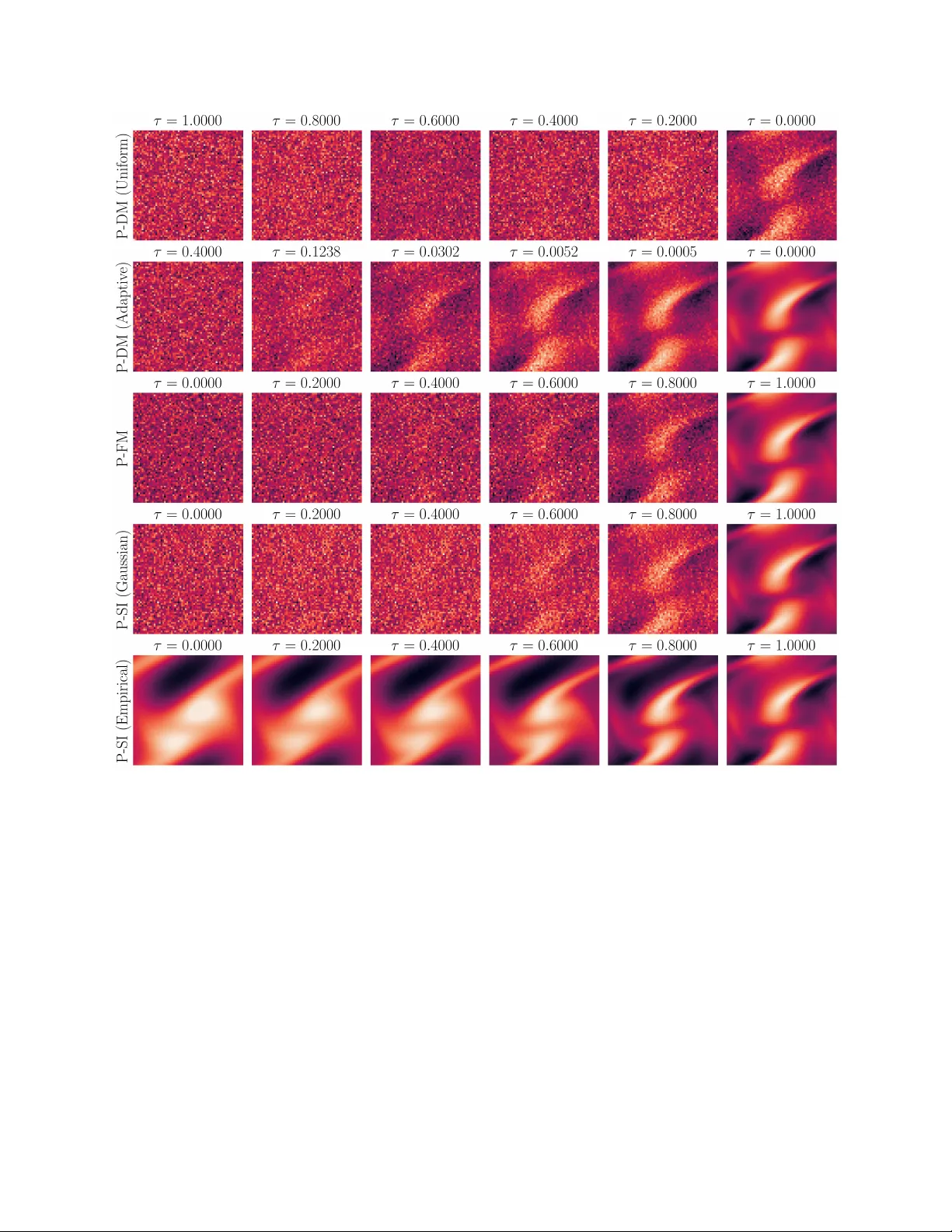
Synergizing T ransp ort-Based Generativ e Mo dels and Laten t Geometry for Sto c hastic Closure Mo deling Xinghao Dong , Huc hen Y ang , Jin-Long W u ∗ Dep artment of Me chanic al Engine ering, University of Wisc onsin–Madison, Madison, WI 53706 Abstract Diﬀusion mo dels recen tly dev elop ed for generativ e AI tasks can pro duce high-qualit y sam- ples while still maintaining div ersit y among samples to promote mo de co v erage, pro viding a promising path for learning sto c hastic closure mo dels. Compared to other t yp es of generativ e AI models, such as GANs and V AEs, the sampling sp eed is known as a k ey disadv an tage of diﬀusion mo dels. By systematically comparing transp ort-based generative mo dels on a n u- merical example of 2D Kolmogoro v ﬂows, we sho w that ﬂo w matc hing in a low er-dimensional laten t space is suited for fast sampling of sto c hastic closure mo dels, enabling single-step sam- pling that is up to t wo orders of magnitude faster than iterative diﬀusion-based approaches. T o con trol the latent space distortion and thus ensure the physical ﬁdelit y of the sampled clo- sure term, we compare the implicit regularization oﬀered by a join t training sc heme against t wo explicit regularizers: metric-preserving (MP) and geometry-aw are (GA) constrain ts. Be- sides oﬀering a faster sampling sp eed, b oth explicitly and implicitly regularized latent spaces inherit the key top ological information from the lo w er-dimensional manifold of the original complex dynamical system, which enables the learning of sto c hastic closure mo dels without demanding a h uge amount of training data. Keywor ds: T urbulence closure, Deep generative model, Latent space, Stochastic model, Non-lo cal model 1. In tro duction Complex dynamical systems, suc h as turbulent ﬂows [ 1 ] or solid mechanics [ 2 ] in engineering applications and physical processes in the Earth system [ 3 ], are often featured b y in teractions across v ast and con tin uous scales of space and time. The computational cost of fully resolving ev ery scale in a Direct Numerical Simulation (DNS) is often prohibitive [ 4 ] for real-w orld science and engineering problems, and practical n umerical simulations need to rely on closure mo dels to appro ximate the impact of unresolv ed, small-scale dynamics on the n umerically resolv ed coarse-grained v ariables. Most existing methods, e.g., RANS or LES closures for mo deling turbulence, rely on a deterministic assumption, whic h only approximately holds if ∗ Corresp onding author Email addr ess: jinlong.wu@wisc.edu (Jin-Long W u) the unresolved scales achiev e equilibrium in a time scale m uch faster than the one that those resolv ed scales ev olve with. Ho wev er, such a separation b et ween resolv ed and unresolv ed scales may not exist for certain problems where the unresolv ed scales are far from equilibrium, motiv ating recent studies of going b ey ond the deterministic closures and exploring sto c hastic mo deling approac hes [ 5 ]. Sto c hastic mo deling has been explored for complex dynamical systems such as turbulence, for several decades [ 6 , 7 ], leading to the dev elopmen t of sto c hastic mo dels for some complex features of turbulent ﬂo ws, e.g., in termittency [ 8 ] and back scattering [ 9 ]. Starting around the millennium, a substan tial amoun t of researc h ab out stochastic mo dels w as explored for geophysical ﬂows [ 10 – 12 ], with an excellen t review of sto chastic mo deling for w eather and climate presen ted b y [ 13 ]. In the mean time, stochastic mo deling tec hniques suc h as random matrices w ere also explored in solid mec hanics [ 14 ] to accoun t for the mo del uncer- tain ties. More recen tly , mesoscale stochastic approaches were explored in the modeling of man y complex systems, suc h as metallic foams [ 15 ] and cellular in teractions [ 16 ]. F rom a broader p ersp ectiv e, sto c hasticit y naturally shows up in reduced-order mo deling tec hniques suc h as Mori-Zwanzig formalism, which demonstrates that when fast-ev olving v ariables are in tegrated out of a system, their inﬂuence on the slow v ariables manifests as b oth a mo diﬁed deterministic force and essen tial memory (non-Mark ovian) and stochastic noise terms [ 17 , 18 ]. In practice, sto c hastic parameterizations hav e b een sho wn to sharp en mean predictions, re- store ph ysical multi-modal v ariability , and repro duce the hea vy-tailed statistics of extreme ev ents across a wide range of applications [ 13 , 19 – 24 ]. Ho w ev er, dev eloping and calibrating sto c hastic closures present their own signiﬁcant challenges [ 25 – 28 ], whic h often p ose a more complicated mo del structure than classical deterministic closures and th us underscore the need for b oth a larger amoun t of data and a more sophisticated calibration pro cedure. This need can b e addressed b y the gro wing ﬁeld of scien tiﬁc mac hine learning (SciML), whic h seeks to augment or replace traditional scien tiﬁc mo deling pip elines with mac hine learning tec hniques [ 29 – 32 ]. Broadly , SciML eﬀorts in dynamical systems mo deling follo w t wo main thrusts. The ﬁrst thrust aims to create data-driven surrogates that appro ximate the system’s evolution from data, eﬀectiv ely replacing traditional ph ysics-based mo dels, e.g., via system iden tiﬁcation [ 33 – 36 ] or op erator learning [ 37 – 39 ]. The second thrust [ 40 – 46 ], as the focus of this w ork, uses mac hine-learning-based mo dels not to replace the traditional ph ysics-based solver but to augment it. This is the goal of data-driv en closure mo deling, whic h retains the well-established physical solver for the resolv ed scales and uses a learned mo del for the con tributions from unresolved ones. It is worth noting that many researc h w orks (e.g., [ 40 , 41 ]) in the second thrust adopted a deterministic form of the mac hine- learning-based mo dels, while the recent adv ances in generativ e AI tec hniques op ened up the p ossibilities of systematically constructing and calibrating data-driven sto c hastic closure mo dels [ 44 ]. Among the recen t developmen ts of generativ e AI tec hniques, three k ey paradigms, all united under a general transp ort-based framew ork, ha ve emerged as comp elling solutions: • Score-based Diﬀusion Mo dels transform data into a simple prior distribution (typ- ically Gaussian noise) through a ﬁxed forw ard SDE and then learn to rev erse this pro cess with a learned score function. This approach has b een successfully applied to 2 sto c hastic closure mo deling [ 44 ] and excels at capturing ric h, non-Gaussian p osteriors, but their highly curv ed transp ort paths necessitate slow, iterative sampling with h un- dreds of solv er steps to maintain ﬁdelit y [ 47 – 49 ]. The extension to conditional diﬀusion mo dels has been explored by v arious computational mec hanics problems [ 44 , 50 – 54 ]. • Flo w Matc hing replaces the sto c hastic noising path with a simpler, often linear, in- terp olation b et ween noise and data. It then learns a deterministi c ODE velocity ﬁeld to transp ort samples along these straigh t paths. This form ulation dramatically simpliﬁes the transp ort, enabling high-quality generation in a single step and admitting exact lik eliho o d computation, though p oten tially at the cost of reduced intrinsic randomness [ 55 – 58 ]. • Sto c hastic In terp olan ts provide a unifying p ersp ectiv e, deﬁning a transp ort pro cess that explicitly interpolates b etw een t w o distributions while allo wing for the injection of time-dep enden t noise. This framew ork retains the eﬃcien t, straight paths of FM while restoring the sto c hastic expressiveness and ﬂexibilit y of diﬀusion mo dels [ 59 – 61 ]. These comp elling solutions of generativ e AI techniques, originally dev elop ed for standard ma- c hine learning tasks such as image/video generation, motiv ate a central question of this work: for sto c hastic closure mo deling, where rapid and rep eated sampling is essential, which of these paradigms best navigates the critical trade-oﬀ b et ween sampling sp eed, sample quality , and uncertain ty represen tation? In addition, since the iterative cost of an y transp ort-based sam- pler scales with the dimensionalit y of the space to p erform sampling, a complemen tary strat- egy for addressing their computational b ottlenec ks in volv es shifting exp ensiv e op erations to lo wer-dimensional laten t spaces. Laten t space generativ e mo dels [ 62 – 65 ] oﬀer a promising en- hancemen t through a tw o-stage pip eline: auto enco ders compress high-dimensional data into compact representations, then generativ e pro cesses op erate within this reduced space. F or online closure mo deling, where a new sample is required at each time step of a physics-based sim ulation, this can accelerate the total simulation time by orders of magnitude [ 54 ]. The success of sampling in a latent space, how ev er, is en tirely con tingen t on the qualit y and structure of the learned laten t representation. A standard auto encoder, trained solely to minimize reconstruction error, has no incen tive to preserv e the geometric or statistical structure of the original data manifold, which can p oten tially force the generative mo del to learn muc h more complicated (or ev en ill-p osed) dynamics in the latent space, leading to unsatisfactory training and inaccurate sampling p erformances. T o o vercome this c hallenge, the laten t space must b e explicitly structured. One approach is implicit regularization via end-to-end join t training, which forces the auto enco der to learn a representation aligned with the generativ e task, outp erforming con ven tional tw o-phase metho ds [ 54 ]. How ev er, this oﬀers no direct con trol ov er the resulting geometry . A more principled strategy , which has gained traction in the broader machine learning comm unity , is to emplo y explicit regularizers during auto encoder training. These metho ds enforce desired inductiv e biases, suc h as spatial equiv ariance [ 66 ], m ultiscale consistency via w av elet-based p enalties [ 67 ], or geometric alignmen t through contrastiv e losses [ 68 , 69 ]. In this work, w e study tw o types of regularizer: geometry-a ware (GA) regularization and metric-preserving (MP) constrain ts. These techniques craft a laten t space that mirrors the geometric and 3 top ological features of the original data, directly impro ving the eﬃciency and accuracy of generativ e mo dels for sto c hastic closure applications. T o summarize, this pap er mak es the following key con tributions: • W e p erform the ﬁrst systematic comparison of diﬀusion, ﬂow matching, and stochas- tic in terp olan t paradigms for sto c hastic closures. W e sho w that ﬂow-based methods ac hieve sup erior sampling sp eed via straighter transp ort paths, enabling order-of- magnitude reductions in the n umber of integration steps with minimal error increase. • W e demonstrate that naive, reconstruction-only auto enco ders introduce signiﬁcan t ge- ometric distortions that scatter conditional distributions. W e sho w that b oth implicit (join t training) and our prop osed explicit (MP , GA) regularization strategies mitigate these issues, yielding structured latent spaces with quan tiﬁable reductions in distortion and impro ved sample ﬁdelity . • W e show that the resulting regularized latent generators in tegrate seamlessly in to ph ysics-based solv ers, deliv ering eﬃcient uncertaint y quantiﬁcation that repro duces full-system statistics while accelerating o verall simulation time. 2. Metho dology W e consider spatiotemp oral dynamical systems, such as those describing turbulent ﬂows and w eather patterns, gov erned b y the full-order equations: ∂ v ∂ t = M ( v ) , (1) where v ∈ V denotes the state encompassing all scales and M is the nonlinear dynamical op erator. The v ast range of scales often renders full resolution computationally intractable, necessitating reduced-order form ulations that evolv e only the resolv ed state, V = P ( v ) : ∂ V ∂ t = M ( V ) + C ( V ) . (2) Here, P is a pro jection op erator (e.g., a low-pass ﬁlter or encoder mapping) and M is the pro jected dynamical op erator. The closure op erator, C , is necessary b ecause the pro jection P do es not comm ute with the nonlinear dynamics M . This non-comm utation means that the evolution of the resolved state V dep ends on interactions with the unresolv ed scales. The closure term, U = C ( V ) , models the net eﬀect of these missing ph ysical in teractions—suc h as energy backscatter and turbulent dissipation—and is essential for restoring ﬁdelit y to the reduced system. T raditional approac hes that parameterize U with simple deterministic or sto chastic func- tions often fail to capture its complex, non-Gaussian, and history-dep enden t nature. A more p o w erful, data-driv en approach is to treat the closure term as a random ob ject and learn 4 its full conditional distribution, p ( U | V ) , from high-ﬁdelit y data. T o ac hieve a ric h, sto c has- tic form ulation, w e can conceptualize the closure term U itself as a sto c hastic ﬁeld whose dynamics ev olve according to: ∂ U ∂ t = H ( U ; V ) + ξ , (3) where H encompasses the op erators go verning the ev olution of U conditioned on the resolv ed state V , and ξ represen ts a sto c hastic forcing term. Rather than explicitly learning the com- plex Sto chastic P artial Diﬀerential Equation (SPDE) in Eq. ( 3 ), we adopt a transp ort-based generativ e mo deling approach to directly characterize the stationary conditional distribution p ( U | V ) that results from these dynamics. This approac h w as ﬁrst pioneered using laten t-space score-based diﬀusion mo dels, whic h demonstrated its viabilit y for this task [ 44 , 54 ]. Ho wev er, these foundational studies also highligh ted the need for faster sampling paradigms to b e practical in online sim ulations and for more robust latent space represen tations to ensure ph ysical ﬁdelity . T o address these c hallenges, w e dev elop a comprehensive framew ork in this section. W e b egin in Section 2.1 b y systematically comparing three transp ort-based generativ e paradigms—diﬀusion models, ﬂo w matching, and sto chastic interpolants—to identify the optimal balance of sp eed and accuracy . Then, in Section 2.2 , we in tro duce and ev aluate several strategies for crafting geometrically structured laten t spaces to enhance the physical consistency of the generated closures. 2.1. T ransp ort-based Laten t Generative Mo dels for Sto c hastic Closures While score-based diﬀusion mo dels, ﬂo w matc hing, and sto c hastic interpolants all op erate by learning a map from a simple prior distribution to a complex target distribution, they diﬀer fundamen tally in their transp ort mec hanisms. These diﬀerences in ho w they mov e probability mass result in distinct sampling pro cedures, computational demands, and training ob jectiv es. The paradigms span a sp ectrum from sto chastic to deterministic transp ort and from highly curv ed to linear sampling paths. 2.1.1. Score-based Diﬀusion Mo dels Score-based diﬀusion mo dels are a class of generativ e mo dels that pro duce samples b y re- v ersing a predeﬁned noise-injection pro cess. The framew ork consists of t wo parts: a ﬁxed forw ard pro cess that gradually p erturbs data in to noise via a Sto c hastic Diﬀeren tial Equa- tion (SDE), and a learned rev erse pro cess that transforms noise bac k in to data b y solving a corresp onding rev erse-time SDE. The forw ard process maps a data sample x 0 ∼ p data ( x ) to a noise v ector o ver a con tinuous time in terv al τ ∈ [0 , T] . A common choice is the V ariance-Explo ding (VE) SDE [ 48 ]: d x = σ τ d W , (4) where σ > 1 is a hyperparameter and W is a standard Wiener pro cess. This forward pro cess is a sp ecial case of the Ornstein–Uhlenbeck pro cess and deﬁnes a Mark ov chain with an analytical transition k ernel: p ( x τ | x 0 ) = N ( x τ | µ ( x 0 , τ ) , Σ ( τ )) , (5) 5 where µ ( x 0 , τ ) = x 0 , Σ ( τ ) = 1 2 log σ  σ 2 τ − 1  I . (6) As τ → T , the distribution p ( x τ ) approaches an isotropic Gaussian independent of the original data, from whic h we can easily sample: p ( x T ) = Z p ( x 0 ) p ( x T | x 0 )d x 0 ≈ N  0 , 1 2 log σ  σ 2T − 1  I  . (7) A known result from sto c hastic calculus states that this forward p rocess has a corresp onding rev erse-time SDE, which allows us to rev erse the noising pro cess to generate data [ 70 ]: d x = − σ 2 τ ∇ x τ log p ( x τ )d τ + σ τ d W , (8) where d W is a Wiener pro cess running bac kw ard in time. Critically , solving this SDE requires the score function, ∇ x τ log p ( x τ ) , of the marginal noisy data distribution p ( x τ ) , whic h is intractable. The cen tral task is therefore to learn a neural netw ork, s θ ( τ , x τ ) , to appro ximate this score. This is achiev ed via denoising score matc hing, where the netw ork is trained to predict the score of the analytically kno wn conditional distribution p ( x τ | x 0 ) . The training ob jectiv e minimizes the weigh ted squared error betw een the net work’s output and the conditional score: min θ E τ , x 0 , x τ  λ ( τ ) ∥ s θ ( τ , x τ ) − ∇ x τ log p ( x τ | x 0 ) ∥ 2 2  , (9) where λ ( τ ) is a p ositiv e w eighting function that balances the loss across diﬀeren t noise lev els to impro ve training stability . F or many diﬀusion setups, this simpliﬁes to setting the w eighting equal to the v ariance of the added noise, i.e. λ ( τ ) = Σ ( τ ) . The conditional score is simply − ( x τ − x 0 ) / Σ( τ ) . This ob jectiv e is tractable as it relies only on samples from the forw ard pro cess and has b een shown to b e equiv alen t to matching the true marginal score [ 71 , 72 ]. Once trained, s θ is used as a plug-in estimator for the true score in Eq. ( 8 ). New samples are generated by starting with x T dra wn from the Gaussian prior and n umerically integrating the SDE bac kward in time, for instance with an Euler-Maruyama solver. This iterative sampling pro cedure is p o w erful but computationally exp ensiv e, often requiring hundreds of steps to main tain ﬁdelity due to the curved nature of the diﬀusion paths. F or conditional mo deling of p ( x | y ) , the framew ork is extended b y mo difying the score net- w ork to accept the condition y as an additional input. During eac h training step, a data pair ( x 0 , y ) is sampled, and the forward noising pro cess is applied only to x 0 . The s core net work s θ ( τ , x τ , y ) then uses both the noisy data and the clean condition to predict the score, with the training ob jectiv e remaining analogous to the unconditional case, except that initial samples are drawn from the join t distribution p ( x , y ) . In addition, the forw ard diﬀusion pro cess acts exclusively on the target v ariable x , meaning the p erturbing kernel p ( x τ | x 0 ) is conditionally indep enden t of an y input condition y . Th us, the training loss b ecomes: θ ∗ = arg min θ E τ , ( x 0 , y ) , x τ  λ ( τ ) ∥ s θ ( τ , x τ , y ) − ∇ x τ log p ( x τ | x 0 ) ∥ 2  , (10) where exp ectations are tak en o ver τ ∼ U [0 , T ] , ( x 0 , y ) ∼ p ( x , y ) , and x τ ∼ p ( x τ | x 0 ) . 6 2.1.2. Flo w Matching Flo w Matc hing (FM) is a paradigm for training contin uous-time generative mo dels that a voids the complexities of SDEs b y learning a deterministic velocity ﬁeld v θ . This learned ﬁeld deﬁnes an Ordinary Diﬀeren tial Equation (ODE) that transp orts samples from a simple prior distribution to the target data distribution. The core idea is to deﬁne a probability path p τ ( x ) that transitions from a prior p 0 ( x ) ≈ N ( 0 , I ) at τ = 0 to the data distribution p 1 ( x ) = p data ( x ) at τ = 1 . This path is generated b y a true, underlying marginal velocity ﬁeld v ( τ , x ) . Ideally , one would train the neural net work v θ b y directly minimizing the discrepancy b et ween it and this true ﬁeld: L FM ( θ ) = E τ ∼U [0 , 1] , x τ ∼ p τ ( x ) ∥ v θ ( τ , x τ ) − v ( τ , x τ ) ∥ 2 2 . (11) Ho wev er, this ob jective is intractable b ecause b oth the marginal probability path p τ ( x ) and its v elo cit y ﬁeld v ( τ , x ) are unkno wn. Conditional Flo w Matching (CFM) resolves this issue with a key insight: instead of working with intractable marginal paths, we can deﬁne a simple, tractable conditional path and v elo cit y ﬁeld, and train the mo del to matc h those instead [ 56 , 58 ]. Sp eciﬁcally , we deﬁne a path conditioned on a sample from the prior, x 0 ∼ p 0 ( x ) , and a sample from the data, x 1 ∼ p data ( x ) . A common and eﬀective choice is a linear in terp olation path: p ( x τ | x 0 , x 1 ) = δ ( x τ − [(1 − τ ) x 0 + τ x 1 ]) , (12) whic h has a simple, constant conditional velocity: v ( τ , x τ | x 0 , x 1 ) = x 1 − x 0 . (13) The cen tral theorem of CFM shows that a loss deﬁned on these simple conditional quantities has the same exp ected gradien t as the intractable marginal loss. This leads to a practical and eﬃcien t training ob jectiv e: min θ E τ , x 0 , x 1 ∥ v θ ( τ , (1 − τ ) x 0 + τ x 1 ) − ( x 1 − x 0 ) ∥ 2 2 . (14) This ob jective is a simple regression problem that do es not require simulating an ODE during training. Once the velocity ﬁeld v θ is trained, new samples are generated b y solving the initial v alue problem for the generation ODE, starting from a random sample x 0 ∼ p 0 ( x ) : d x dτ = v θ ( τ , x ) , for τ ∈ [0 , 1] . (15) This ODE can b e solved with standard numerical in tegrators, such as the Euler metho d. Because the training encourages nearly straight transp ort paths, FM mo dels are highly eﬃ- cien t at inference, often requiring only 10–100 steps for high-qualit y generation—a signiﬁcant sp eed-up o v er typical diﬀusion mo dels. F or conditional mo deling of p ( x | y ) , the velocity netw ork is simply mo diﬁed to accept the condition y as an additional input, v θ ( τ , x τ , y ) . The training ob jectiv e in Eq. ( 14 ) is adapted b y sampling from the joint data distribution ( x 1 , y ) ∼ p ( x , y ) . 7 2.1.3. Sto c hastic Interpolants Sto c hastic In terp olan ts (SI) oﬀer a unifying and highly ﬂexible paradigm for generativ e mo deling that generalizes b oth diﬀusion mo dels and ﬂo w matching [ 59 ]. The core idea is to explicitly deﬁne a sto c hastic path, or in terp olan t, that connects any arbitrary source distribution p 0 ( x 0 ) to the target data distribution p 1 ( x 1 ) , and then learn the drift of the SDE that generates this path. F ormally , the interpolant path betw een a pair of samples ( x 0 , x 1 ) is deﬁned as: x τ = α τ x 0 + β τ x 1 + σ τ W τ , τ ∈ [0 , 1] , (16) where W τ is a standard Wiener pro cess and the co eﬃcien ts ( α τ , β τ , σ τ ) satisfy the b oundary conditions x τ =0 = x 0 and x τ =1 = x 1 . The SI framew ork pro vides a simple and eﬃcient training ob jectiv e based on this path. W e ﬁrs t deﬁne a path v elo cit y r τ , whic h includes a drift term that arises from the time-v arying noise schedule: r τ = ˙ α τ x 0 + ˙ β τ x 1 + ˙ σ τ W τ , (17) where the dot denotes a time deriv ative. The neural net w ork b θ ( τ , x τ ) , whic h appro ximates the drift of the forward SDE, is trained via a simple regression ob jectiv e to predict this path v elo cit y: min θ E τ , x 0 , x 1 , W τ ∥ b θ ( τ , x τ ) − r τ ∥ 2 2 . (18) A common choice that encourages straigh t mean paths is the linear in terp olan t , where α τ = 1 − τ and β τ = τ . In this case, the deterministic part of the path v elo cit y simpliﬁes to the constan t vector x 1 − x 0 . The full path velocity , ho wev er, retains its sto c hastic comp onen t, whic h dep ends on the c hosen noise schedule. F or example, with a simple noise schedule of σ τ = 1 − τ , we hav e ˙ σ τ = − 1 , and the full path velocity b ecomes: r τ = x 1 − x 0 − W τ . (19) This ob jective mirrors Conditional Flo w Matching but crucially incorp orates the sto c hastic drift term, allo wing for tunable noise injection. Once trained, new samples are generated b y n umerically in tegrating the learned forw ard SDE, starting with a sample from the prior: d x τ = b θ ( τ , x τ )d τ + σ τ d W τ , x 0 ∼ p 0 ( x ) , (20) F or conditional mo deling of p ( x | y ) , the drift netw ork is mo diﬁed to b θ ( τ , x τ , y ) and trained on samples from the join t distribution p ( x 1 , y ) . A k ey adv antage of the SI framework is its ﬂexibilit y in c ho osing the source distribution p 0 . While d iﬀusion and standard FM typically use a ﬁxed Gaussian prior, SI can directly in terp o- late b et w een t wo arbitrary distributions. This is particularly p o w erful for closure modeling. Instead of starting from random noise, w e can set the source distribution to b e the condi- tional v ariable itself, p 0 ( x 0 ) = p ( z ω ) , and the target to be the closure, p 1 ( x 1 ) = p ( z H | z ω ) . The model then learns the direct, ph ysically meaningful transp ort from the resolv ed state to the unresolv ed correction term. 8 2.2. Crafting Structured Laten t Spaces for Generativ e Closures Deplo ying transp ort-based generative mo dels for sto c hastic closures is computationally c hal- lenging due to the high dimensionality of the discretized ph ysical ﬁelds. The iterativ e sam- pling pro cess can be prohibitively exp ensiv e when p erformed in the full state space. T o mitigate this cost, we emplo y a laten t space approac h, using a con v olutional autoenco der to learn a lo w-dimensional representation of the data. Giv en a physical ﬁeld U (with the conditioning ﬁeld V treated analogously), the enco der E U maps it to a compact laten t vector: z U = E U ( U ) , where U ∈ R d U and z U ∈ R l U with l U ≪ d U . (21) The deco der D U then reconstructs an approximation of the original ﬁeld from this laten t v ector, ˆ U = D U ( z U ) . In a conv en tional t w o-phase pip eline, the auto encoder parameters are optimized b y solely minimizing the mean squared reconstruction error: L U Recon = E U ∼ p ( U ) ∥ U − D U ( E U ( U )) ∥ 2 2 . (22) Ho wev er, a latent space optimized only for reconstruction qualit y can b e arbitrarily distorted, as the loss in Eq. ( 22 ) is agnostic to the manifold’s geometric structure. This can scatter conditional distributions and complicate the transp ort paths for a subsequent generative mo del, degrading its p erformance. T o ov ercome this limitation and craft a latent space that is w ell-suited for the generative task, we systematically compare t w o distinct strategies: • End-to-end joint training , where the auto encoder and generative mo del are opti- mized sim ultaneously , providing an implicit r e gularizati on on the laten t space. • T wo-phase training with explicit regularization , where the auto enco der is ﬁrst pre-trained with an ob jectiv e function that directly enforces sp eciﬁc geometric prop er- ties on the laten t space. These approaches aim to create more structured and informativ e laten t spaces that simplify the generativ e task while maintaining high-ﬁdelit y reconstructions. The detailed mo del structures and training details of auto encoders can b e found in App endix C . 2.2.1. Implicit Regularization via Join t T raining An alternativ e to the tw o-phase pip eline is to train the auto encoder and the generative mo del sim ultaneously . This end-to-end joint training serves as a p o w erful implicit regularizer. By receiving gradients from b oth the reconstruction and generativ e ob jectiv es, the auto encoder is forced to learn a laten t space that is not only faithful to the original data but is also struc- tured in a w ay that simpliﬁes the generativ e transp ort task, often outp erforming sequen tial training pip elines [ 73 , 74 ]. The training is guided b y a multi-ob jective loss function, whic h is a w eighted sum of three distinct terms: L joint = L Recon + λ Gen L Gen + λ KL L KL . (23) Eac h comp onen t addresses a diﬀerent requirement of the learning process: 9 • The Reconstruction Loss ( L Recon ) ensures that the auto enco der pro duces high- ﬁdelit y represen tations. It is a w eigh ted mean squared error that often prioritizes the accuracy of the more complex or crucial ﬁeld, which in this case is the closure term U : L Recon = E ( U , V )  λ U ∥ U − D U ( E U ( U )) ∥ 2 2 + λ V ∥ V − D V ( E V ( V )) ∥ 2 2  , (24) where the exp ectation is o v er the data distribution, and typically λ U > λ V . • The Generative Loss ( L Gen ) is the transp ort ob jectiv e that trains the generativ e mo del. This corresp onds to the score-matching, ﬂo w-matching, or drift-regression losses deﬁned in Section 2.1 . • The KL Regularization ( L KL ) preven ts latent collapse, a failure mo de where the enco der maps all inputs to a small, uninformativ e region of the laten t space [ 75 ]. This term encourages the aggregated distribution of enco ded samples, q ( z U ) , to matc h a simple prior, t ypically a standard Gaussian p ( z U ) = N ( 0 , I ) , thereb y ensuring the laten t space remains expressive: L KL = KL  q ( z U ) ∥ p ( z U )  . (25) The h yp erparameters λ Gen and λ KL balance these comp eting ob jectives, and their tuning is critical for ac hieving a mo del that excels at b oth reconstruction and conditional generation. 2.2.2. Explicit Regularization via a T wo-Phase Strategy The second strategy for crafting a well-structured laten t space is to employ explicit regular- ization within a stable, tw o-phase training pip eline. The core idea is to ﬁrst pre-train the auto encoder with an ob jectiv e function that directly enforces desired geometric properties on the laten t space, b efore the generativ e mo del is trained. W e in tro duce and ev aluate tw o suc h regularizers: • Metric-Preserving (MP) Regularization: This approac h aims to mak e the en- co der a lo c al isometry . It seeks to preserv e the direct Euclidean distance b et ween pairs of p oin ts, ensuring that the lo cal "neighborho o d" structure of the ph ysical space is accurately mapp ed to the laten t space. This is akin to "unrolling" the data manifold in to a ﬂat latent representation without locally stretching or tearing it. • Geometry-A ware (GA) Regularization: This approac h aims to preserv e the more global, intrinsic manifold ge ometry . Instead of using the straigh t-line Euclidean dis- tance, it uses a pre-computed manifold distance (approximating the geo desic distance) b et w een points. This captures the true "on-manifold" path length, preserving the larger-scale top ological features of the data. Both strategies are implemen ted b y augmenting the standard reconstruction loss from Eq. ( 22 ) with a structural loss term: L AE = L U Recon + λ Struc L U Struc , (26) 10 where λ Struc is a h yp erparameter that balances reconstruction ﬁdelity with geometric preser- v ation. The structural loss, L Struc , penalizes the discrepancy b et w een distances in the ph ys- ical and laten t spaces, with a fo cus on lo cal neigh b orhoo ds: L Struc = E U i , U j ∼ p ( U )  w ( U i , U j ) ( ∥E U ( U i ) − E U ( U j ) ∥ 2 − d ( U i , U j )) 2  , (27) where the weigh t w ( U i , U j ) = e − γ d ( U i , U j ) emphasizes local pairs. This general form is spe- cialized b y deﬁning the distance metric d ( · , · ) as either the Euclidean norm ( ∥ · ∥ 2 ) for MP reg- ularization or the pre-computed manifold distance for GA regularization. This pre-training phase, applied to the auto enco ders for b oth the closure and conditioning ﬁelds, pro duces laten t represen tations that retain the intrinsic structure of the data, thereby simplifying the subsequen t generative mo deling task. 3. Numerical Results 3.1. Numerical Setup W e ev aluate our generative closure framew ork on a tw o-dimensional sto c hastic Kolmogoro v ﬂo w. The system is go verned b y the incompressible Navier-Stok es equations in vorticit y form on a p eriodic domain Ω = (0 , L ) 2 o ver the time interv al (0 , T phy ] : ∂ ω ( x , t ) ∂ t = − u ( x , t ) · ∇ ω ( x , t ) + f ( x ) + ν ∇ 2 ω ( x , t ) + β ξ ( x , t ) , ∇ · u ( x , t ) = 0 , ω ( x , 0) = ω 0 ( x ) . (28) Here, ω is the vorticit y , u is the divergence-free velocity ﬁeld, and ν = 10 − 3 is the vis- cosit y . The system is initialized with a random v orticit y ﬁeld ω 0 dra wn from a statisti- cally stationary Gaussian distribution and is driv en by a deterministic, large-scale forcing f ( x ) = 0 . 1(sin(2 π ( x + y )) + cos(2 π ( x + y ))) . A high-frequency sto c hastic term ξ , representing white-in-time noise with amplitude β = 5 × 10 − 5 , is included to mimic unresolved physical ﬂuctuations. Our data-driv en closure task is to learn a mo del for the unresolved subgrid-scale dynamics. W e deﬁne the closure term, H , as the com bination of the nonlinear adv ection and the sto c hastic forcing, b oth of whic h are considered unkno wn to the coarse-grained mo del: H ( x , t ) = − u ( x , t ) · ∇ ω ( x , t ) + β ξ ( x , t ) . (29) The goal is to learn a generativ e mo del for the conditional distribution p ( H | ω ) . T o generate the training dataset, w e p erform 100 indep enden t high-ﬁdeli t y sim ulations of Eq. ( 28 ) on a ﬁne 256 × 256 grid using a pseudo-sp ectral metho d with a Crank-Nicolson time- stepping sc heme ( ∆ t = 10 − 3 ). T o ensure the data represents a statistically stationary state, w e discard the initial 30 seconds of eac h simulation. The remaining solutions are spatially do wnsampled to a coarse 64 × 64 grid and temp orally subsampled at 0.01-second interv als. This process yields a ﬁnal dataset of 20,000 pairs, consisting of the resolv ed vorticit y ﬁelds ω (the conditional input) and the corresp onding subgrid closure terms H (the prediction target). This dataset is then split into 18,000 pairs for training and 2,000 for testing. 11 3.2. Exp erimen tal Design and Comparativ e F ramew ork In the following sections, we presen t a systematic comparison to ev aluate the p erformance of diﬀeren t transp ort-based generative closures. Our experimental framew ork is designed as a matrix of comparisons b et w een three core generativ e paradigms and ﬁv e distinct data represen tation and training strategies. The three generativ e paradigms under inv estigation are: (i) Score-based Diﬀusion Mo dels (DM): An SDE-based sto c hastic approac h that rev erses a ﬁxed noising pro cess. (ii) Flo w Matc hing (FM): A deterministic ODE-based approac h that learns a v elo cit y ﬁeld along straigh t interpolation paths. (iii) Sto c hastic In terp olan ts (SI): A ﬂexible hybrid framework. W e ev aluate this paradigm using tw o distinct source distributions: a standard Gaussian prior and an empirical prior deriv ed from the conditioning v ariable itself. Eac h of these paradigms is applied across the following ﬁve data represen tation and training strategies: (i) Ph ysical Space: A baseline mo del operating directly on the full-resolution 64 × 64 ﬁelds. (ii) Laten t Space (No Regularization): A t wo-phase mo del using a standard, reconstruction- only auto encoder on 16 × 16 laten t ﬁelds. (iii) Laten t Space (Join t T raining): An end-to-end trained mo del with implicit regu- larization on the 16 × 16 latent ﬁelds. (iv) Laten t Space (Metric-Preserving): A t wo-phase mo del with explicit MP regular- ization applied during auto encoder pre-training. (v) Laten t Space (Geometry-A ware): A tw o-phase mo del with explicit GA regular- ization applied during auto encoder pre-training. The p erformance of each combination is ev aluated based on quan titativ e error metrics, the preserv ation of physical statistics (e.g., energy sp ectra), and computational cost. 3.3. P erformance in Ph ysical Space: A Baseline for Comparison This section establishes a p erformance baseline for the three transport-based generativ e paradigms. All mo dels are trained and ev aluated directly on the full-resolution 64 × 64 ph ysical-space data. W e denote these mo dels with a "P-" preﬁx (e.g., P-DM, P-FM, P-SI) to distinguish them from the laten t-space v arian ts analyzed in subsequent sections. T o assess b oth the predictive accuracy and the uncertaint y representation of eac h paradigm, w e p erform an ensemble-based analysis. F or a giv en conditional input ω , we draw an ensem- ble of N s = 1000 closure samples { ˜ H i } N s i =1 from the learned conditional distribution p θ ( H | ω ) . The accuracy of the model is ev aluated using the ensem ble mean, ¯ H = 1 N s P N s i =1 ˜ H i , which 12 represen ts the mo del’s deterministic b est guess. The mo del’s predicted uncertain t y is c har- acterized b y the p oint wise standard deviation of the ensemble, whic h is compared against the ground-truth v ariability . W e quantify the error of the ensem ble-mean prediction against the ground truth H using t wo metrics: the Mean Squared Error (MSE) and the Relativ e Error (RE), deﬁned as: D MSE = 1 N p ∥ ¯ H − H ∥ 2 F , (30) and D RE = ∥ ¯ H − H ∥ F ∥ H ∥ F , (31) where ∥ · ∥ F is the F rob enius norm and N p is the total n umber of grid p oin ts in the ﬁeld. Figure 1: Qualitativ e comparison of sto c hastic closure samples from ph ysical-space mo dels. This ﬁgure assesses the p erformance of conditional generation. Each column corresp onds to a diﬀeren t model: the ground truth, P-DM, P-FM, and P-SI with tw o diﬀerent priors. Each row displa ys an indep enden t, random sample of the closure term H , all generated for the same input vorticit y ﬁeld ω . W e ﬁrst ev aluate the qualitativ e p erformance of the physical-space mo dels. As sho wn in Figure 1 , all three paradigms (DM, FM, and SI) generate high-ﬁdelity , div erse samples of the closure term H . The generated samples are structurally consisten t with the ground truth, demonstrating that the mo dels ha v e learned a meaningful conditional distribution. F or a quantitativ e analysis, T able 1 rep orts sev eral key metrics. The ensemble-mean errors ( D ens RE ), whic h measure how well each mo del captures the deterministic component of the closure, are comparable across all metho ds, ranging from 8.6% to 9.0%. This conﬁrms that all paradigms are highly eﬀectiv e at this task, with the P-SI mo dels showing a marginal 13 T able 1: Quantitativ e comparison of physical-space generative mo dels. All metrics are av eraged ov er the test set. Per-sample errors measure the av erage error of individual sto c hastic draws, while ensemble-mean errors measure the accuracy of the av eraged prediction. Field Std. is the spatially-a veraged standard deviation of the generated ensemble, indicating the magnitude of mo deled uncertain ty . V alues in gra y denote ± tw o standard deviation ov er the test set instances. Mo dels Mean of p er-sample errors Error of ensemble mean Field Std. D sample MSE D sample RE D ens MSE D ens RE P-DM 8.231e-04 ± 1.185e-04 1.157e-01 ± 8.451e-03 4.696e-04 8.725e-02 1.885e-02 ± 2.702e-03 P-FM 9.340e-04 ± 1.165e-04 1.231e-01 ± 7.484e-03 5.051e-04 9.028e-02 2.074e-02 ± 3.390e-03 P-SI (Gaussian) 8.831e-04 ± 1.184e-04 1.199e-01 ± 7.951e-03 4.541e-04 8.595e-02 2.076e-02 ± 3.162e-03 P-SI (Empirical) 8.732e-04 ± 1.266e-04 1.192e-01 ± 8.591e-03 4.566e-04 8.610e-02 2 .050e-02 ± 2.501e-03 adv antage. As exp ected, these errors are consistently low er than the a verage p er-sample errors due to the v ariance-reduction eﬀect of av eraging. Crucially , the table also allows us to ev aluate how w ell the models represen t the prescribed sto c hasticit y via the spatially-av eraged standard deviation (Field Std.). F or our problem setup, this quantit y has an analytical reference v alue of 0.02 (see App endix B ). All mo dels repro duce this target with high ﬁdelity; the P-FM and P-SI mo dels match the ground-truth v ariance almost exactly , while the P-DM sligh tly underestimates it, though all are within a 10% relativ e error. Accurately capturing the uncertain t y level is critical for preserving the system’s physical statistics in forward sim ulations. These com bined results establish that all ph ysical-space generativ e paradigms p erform well, accurately capturing b oth the mean b eha vior and the uncertain ty level of the closure. 3.4. The Role of T ransp ort Geometry in Sampling Eﬃciency While the previous section established that all generativ e paradigms achiev e comparable accuracy with a suﬃcient n umber of sampling steps, their computational eﬃciency v aries dramatically . As sho wn in T able 2 , reducing the n umber of integration steps causes the accuracy of the P-DM mo del to degrade sharply , with a catastrophic failure at a single step. In con trast, the linear-interpolation-based P-FM and P-SI mo dels remain remark ably stable, with P-FM sho wing almost no loss in accuracy even in the single-step regime. T able 2: Sampling accuracy vs. num b er of integration steps. Linear-in terp olation–based metho ds (P-FM, P-SI) remain stable with far fewer steps, while the P-DM mo del degrades sharply under coarse discretization. Sample steps P-DM P-FM P-SI Gaussian priors Empirical priors D MSE D RE D MSE D RE D MSE D RE D MSE D RE 100 7.945e-04 1.197e-01 7.228e-04 1.112e-01 8.776e-04 1.254e-01 8.576e-04 1.244e-01 50 7.431e-03 3.158e-01 8.025e-04 1.197e-01 8.736e-04 1.250e-01 8.641e-04 1.249e-01 10 3.130e-02 7.563e-01 8.796e-04 1.200e-01 8.971e-04 1.269e-01 9.390e-04 1.298e-01 1 8.262e+02 2.851e+02 9.846e-04 1.334e-01 3.434e-03 2.502e-01 2.845e-03 2.265e-01 This diﬀerence in robustness is a direct consequence of the underlying transp ort path ge- ometry . T o quan tify this, we deﬁne a straigh tness metric S ∈ [0 , 1] that measures the ratio 14 of the direct Euclidean distance b et w een a tra jectory’s start and end p oin ts to the total in tegrated path length (a v alue of S = 1 indicates a p erfectly straight line). T able 3 conﬁrms the link b et ween path geometry and sampler stability . P-FM follo ws almost p erfectly linear paths ( S ≈ 0 . 999 ), explaining its tolerance to large step sizes. In con trast, P-DM traces highly curved paths ( S < 0 . 3 ), which require ﬁne discretization to integrate accurately . P-SI o ccupies a middle ground, consisten t with its moderate stabilit y . The S = 1 v alues for all mo dels at a single step are a geometric artifact, as a one-step path is trivially straight but not necessarily accurate. Th us, high S m ust b e interpreted in conjunction with accuracy metrics to assess practical eﬃciency . T able 3: T ra jectory straigh tness ( S ) for diﬀeren t sampling metho ds. Higher v alues ( → 1 ) indicate straigh ter paths. P-FM’s near-p erfect straightness explains its robustness to coarse time discretization. Sample steps P-DM P-FM P-SI Gaussian priors Empirical priors 100 1.278e-01 ± 2.467e-03 9.995e-01 ± 1.881e-04 1.929e-01 ± 3.938e-03 1.857e-01 ± 1.357e-02 50 1.717e-01 ± 3.293e-03 9.995e-01 ± 1.718e-04 2.602e-01 ± 5.120e-03 2.508e-01 ± 1.770e-02 10 2.553e-01 ± 4.854e-03 9.997e-01 ± 1.153e-04 4.524e-01 ± 8.342e-03 4.373e-01 ± 2.716e-02 1 1.000e+00 ± 0.000e+00 1.000e+00 ± 0.000e+00 1.000e+00 ± 0.000e+00 1.000e+00 ± 0.000e+00 Figure 2 visualizes these distinct dynamics and provides crucial insights into sampler design. The standard P-DM sampler with uniform steps (Ro w 1) fails to conv erge in a 10-step budget, as its highly curv ed path cannot b e in tegrated accurately with coarse steps. How ev er, the p erformance of diﬀusion mo dels can b e dramatically impro ved with a more tailored strategy . Ro w 2 shows an adaptiv e P-DM sampler that successfully conv erges in the same 10-step budget. This is achiev ed b y: 1. Reducing Initial V ariance: Since w e are targeting a narrow conditional distribution, the rev erse SDE can b e initialized from a state of lo w er noise (i.e., starting at τ < T ), signiﬁcan tly shortening the required path length. 2. A daptive Time-Stepping: An adaptive sc hedule uses larger steps in the high-noise regime where the path is smo other and smaller steps near the data manifold ( τ → 0 ) where curv ature and stiﬀness increase, thus optimizing the discretization. In con trast, the inherently straighter paths of P-FM (Ro w 3) and P-SI (Rows 4-5) allow them to conv erge smo othly ev en with simple uniform time-stepping, reinforcing the conclusion that path geometry is a primary determinan t of sampling eﬃciency . 3.5. Impact of Laten t Space Geometry on Generative P erformance Laten t generative mo dels oﬀer signiﬁcant computational adv an tages, but their success is critically dep enden t on the qualit y of the laten t space. In this section, we systematically ev aluate ho w diﬀerent auto encoder (AE) training strategies impact the geometry of the latent space and the p erformance of the do wnstream generative closure model. W e compare four families of strategies: tw o-phase training without regularization (NoReg), end-to-end join t training (Joint), and t wo-phase training with explicit metric-preserving (MP) or geometry- a ware (GA) regularization. 15 Figure 2: Visualization of 10-step sampling tra jectories. Eac h row sho ws in termediate states of the generated ﬁeld for a diﬀerent sampling strategy , with time τ evolving according to the mo del’s pro cess. The comparison b etw een the standard P-DM (Row 1) and an adaptive P-DM with reduced initial v ariance (Ro w 2) highlights how sampler design can ov ercome path curv ature. The smo oth evolution of P-FM (Row 3) and P-SI (Rows 4-5) visually conﬁrms their straigh ter transport paths. 3.5.1. The F ailure of Reconstruction-Only Latent Spaces W e ﬁrst establish that a laten t space optimized solely for reconstruction is unsuitable for generativ e mo deling. As sho wn in T able 5 , the NoReg strategy results in catastrophic failure, with a latent-space relativ e error ( D RE ) of approximately 30%, whic h translates to a deco ded ph ysical-space error of 33%—far worse than any of the ph ysical-space baseline mo dels. The reason for this failure is revealed b y the laten t space geometry , visualized in Figure 4 and quantiﬁed in T able 6 . The NoReg auto enco der pro duces a highly distorted latent space, evidenced by its scattered t-SNE em b eddings, large Pro crustes Disparit y (PD), and a nearly 16 threefold increase in the conditional co eﬃcien t of v ariation (CV) compared to the ph ysical space. Crucially , this geometric failure o ccurs despite the NoReg mo del achieving the low est reconstruction error of all tested strategies (T able 4 ). This establishes our central thesis: faithful reconstruction is a necessary but insuﬃcient condition for eﬀectiv e latent generative mo deling; the geometry of the laten t space is paramoun t. 3.5.2. The Eﬃcacy of Implicit and Explicit Regularization Structuring the latent space, either implicitly or explicitly , dramatically improv es p erfor- mance. Joint training provides a p o w erful implicit regularization, forcing the AE to co-adapt with the generative mo del. This alignment yields a massive improv emen t o v er the NoReg baseline, reducing the laten t-space error by o ver 4x and ac hieving a ﬁnal ph ysical-space ac- curacy comparable to the ph ysical-space mo dels (T able 5 ). This p erformance gain is directly link ed to an improv ed laten t geometry with lo wer distortion metrics sho wn in T able 6 . Ho wev er, explicit geometric regularization during a t w o-phase pip eline pro v es to be the most eﬀective and stable strategy . The results in T able 5 are unequiv o cal: the MP and GA regularized mo dels ac hiev e the low est laten t-space generation errors of all metho ds. The MP-regularized mo dels are the top p erformers, yielding the low est latent-space error ( ∼ 2.9%) and a ﬁnal ph ysical-space error ( ∼ 8.3%) that matches or ev en slightly surpasses the ph ysical-space baselines. The sup eriorit y of the explicitly regularized mo dels is corrob orated by the training loss curv es in Figure 3 , which use a normalized Flo w Matc hing (FM) loss for direct comparison. The smo oth, low-loss tra jectories of the MP and GA mo dels indicate that a well-structured latent space makes the generative ob jectiv e fundamentally easier to optimize. In con trast, the Join t mo del’s loss curve, while b etter than NoReg, exhibits a pronounced spike attributed to the non-stationarit y of the co-adapting AE. Of the tw o explicit regularizers, MP consisten tly outp erforms GA in generativ e tasks. The adv antage of MP arises from its direct alignment with the mec hanics of the transp ort-based samplers. Op erations suc h as discretized SDE/ODE in tegration, interpolation, and gradi- en t ev aluation are p erformed in Euclidean coordinates; preserving lo cal Euclidean distances (MP) is therefore more b eneﬁcial than preserving geo desic distances (GA). F urthermore, MP is more computationally eﬃcient, as it requires only pairwise Euclidean distances rather than more exp ensiv e geo desic estimates. In summary , for laten t generative closures, explic- itly regularizing the AE geometry with metric-preserving constrain ts is the most eﬀective, stable, and eﬃcien t strategy . 3.6. A Posteriori V alidation via Numerical Sim ulation T o assess the a p osteriori performance of the generativ e closure framew ork, w e em b ed the trained mo dels within a n umerical solv er for the 2-D Navier-Stok es equations (Eq. ( 28 )). The sim ulations are initialized at t 0 = 30 using a ground-truth vorticit y ﬁeld, ω ( x , t 0 ) , and are in tegrated forward to t = 50 with a time step of ∆ t = 10 − 3 . The solver emplo ys the same pseudo-sp ectral and Crank-Nicolson metho ds used to generate the training data. The system is ev olved with a viscosit y of ν = 10 − 3 and is sub ject to the deterministic forcing 17 T able 4: Auto enco der reconstruction errors. Each blo c k rep orts mean-squared ( D MSE ) and relative ( D RE ) errors. Note that the Recon only baseline has the low est reconstruction error, y et the worst generative p erformance (see T able 5 ). Auto encoders V orticit y ω Con vection H D MSE D RE D MSE D RE Recon only - 5.280e-07 7.382e-04 7.168e-06 1.124e-02 Join t-trained w/ DM 5.772e-06 2.484e-03 4.019e-05 2.439e-02 w/ FM 4.638e-06 2.215e-03 6.265e-06 1.039e-02 w/ SI (Gaussian) 5.041e-05 7.231e-03 3.180e-05 2.219e-02 w/ SI (Empirical) 5.133e-06 2.334e-03 4.419e-06 8.650e-03 Regularized MP 5.571e-05 7.666e-03 2.415e-05 1.844e-02 GA 3.920e-05 6.461e-03 2.592e-05 1.921e-02 T able 5: Generative p erformance across diﬀerent latent space strategies. Physical-space mo dels (P-) are baselines. Latent-space mo dels (L-) sho w that NoReg fails, Join t impro ves signiﬁcantly , and explicit regularization (MP , GA) p erforms b est. Bold v alues highlight the b est p erformance within each category (laten t and physical errors for MP). Mo del Laten t space Ph ysical space generation generation Catagory P aradigms D MSE D RE D MSE D RE Ph ysical space mo dels P-DM - - 4.696e-04 8.725e-02 P-FM - - 4.911e-04 8.904e-02 P-SI (Gaussian) - - 4.612e-04 8.662e-02 P-SI (Empirical) - - 4.994e-04 9.032e-02 Laten t space mo dels T wo-phase w/o regs L-DM 9.524e-02 3.154e-01 6.220e-03 3.290e-01 L-FM 9.501e-02 3.045e-01 6.679e-03 3.302e-01 L-SI (Gaussian) 1.098e-01 3.171e-01 7.030e-03 3.379e-01 L-SI (Empirical) 9.637e-02 2.995e-01 6.716e-03 3.313e-01 Join t-trained L-DM 3.677e-05 7.630e-02 4.877e-04 8.932e-02 L-FM 3.525e-03 7.394e-02 4.862e-04 8.928e-02 L-SI (Gaussian) 2.812e-03 7.290e-02 5.131e-04 9.151e-02 L-SI (Empirical) 3.129e-03 8.274e-01 6.715e-04 9.219e-01 T wo-phase w/ MP L-DM 6.379e-03 2.936e-02 4.224e-04 8.279e-02 L-FM 6.365e-03 2.932e-02 4.243e-04 8.299e-02 L-SI (Gaussian) 6.592e-03 2.982e-02 4.400e-04 8.456e-02 L-SI (Empirical) 6.297e-03 2.852e-02 4.302e-04 8.322e-02 T wo-phase w/ GA L-CDM 2.275e-02 3.801e-02 6.006e-04 9.986e-02 L-FM 1.851e-02 3.439e-02 5.642e-04 9.673e-02 L-SI (Gaussian) 1.869e-02 3.457e-02 5.614e-04 9.660e-02 L-SI (Empirical) 2.223e-02 3.772e-02 5.560e-04 9.526e-02 term f ( x ) = 0 . 1(sin(2 π ( x + y )) + cos(2 π ( x + y ))) . F or computational eﬃciency , the closure term is up dated ev ery ﬁv e physical time steps. W e ev aluate t w o strategies for deploying the sto c hastic closure: (1) Stochastic T ra jectory Sim ulation. T o c haracterize the uncertaint y propagation of the closure, we p erform a Monte Carlo analysis. F or eac h of N e = 1000 indep enden t 18 Figure 3: Normalized Flow Matching (FM) training loss (log-scale). The explicitly regularized mo dels (MP , GA) achiev e the lo west and smo othest loss tra jec tories, indicating that a well-structured latent space simpliﬁes the generative learning task. The Joint mo del exhibits a non-stationary spik e, while the NoReg mo del conv erges to a muc h higher loss. Figure 4: t-SNE visualizations of laten t space structure. Each column represents a diﬀerent training strategy . The unregularized laten t space (Column 2) is visibly distorted compared to the physical space ground truth (Column 1). Joint training (Columns 3-6) and explicit regularization (Columns 7-8) pro duce far more coherent structures. sim ulations, a single closure term ˜ H ( x , t ) is sampled from the conditional distribution p ( H | ω ) at each ev aluation step. The resulting ensemble of tra jectories allows for the computation of statistics, suc h as the mean and standard deviation of prediction errors. (2) Conditional Mean Simulation. T o obtain a deterministic prediction that minimizes v ariance, we approximate the conditional exp ectation of the closure term. At each ev aluation step, we draw a large ensem ble of N e = 1000 samples, { ˜ H i } N e i =1 ∼ p ( H | ω ) , and compute 19 T able 6: Quantitativ e assessment of laten t space distortion using Pro crustes disparit y (PD) and mean of absolute CV. PD measures geometric dissimilarity b et ween t-SNE em b eddings after optimal alignmen t—low er v alues indicate b etter preserv ation of data structure. Mean of absolute CV quantiﬁes the relativ e spread of conditional distributions p ( H | ω ) —lo wer v alues indicate more compact conditionals. Bold v alues indicate b est p erformance p er metric. Distributions Metrics Spaces Physical T wo-phase Join t Joint Joint Joint T wo-phase T wo-phase Space w/o Reg w/ DM w/ FM w/ SI (Gaussian) w/ SI (Empirical) w/ MP w/ GA p ( ω ) PD – 5.370e-01 9.855e-03 1.215e-02 1.434e-02 1.371e-02 1.561e-02 6.710e-02 p ( H ) PD – 1.637e-01 2.130e-02 2.835e-02 4.302e-02 9.609e-02 3.772e-03 3.938e-02 p ( H, ω ) PD – 2.567e-01 1.003e-01 8.162e-02 7.826e-02 1.016e-01 1.024e-01 9.534e-03 p ( H | ω ) Mean of absolute CV 2.571e-01 7.562e-01 1.245e-01 2.378e-01 2.365e-01 1.9092e-01 5.147e-02 1.074e-01 their mean, ¯ H = 1 N e P N e i =1 ˜ H i . This mean v alue is then used as the closure term for a single sim ulation tra jectory . Results summarized in T able 7 and Figure 5 conﬁrm the critical role of the closure term. The uncorrected simulation exhibits rapid error accumulation, with the relativ e error ( D RE ) reac hing 84.2% by t = 50 . In contrast, all generativ e closure mo dels successfully mitigate this error growth, main taining a ﬁnal error b elo w 13%. The qualitativ e impact of this correction is visualized in Figure 6 , where the vorticit y ﬁeld from the corrected sim ulation remains structurally coheren t and aligned with the high-ﬁdelity reference, unlik e the uncorrected ﬁeld whic h diverges signiﬁcantly in both pattern and magnitude. Notably , the mo dels featuring structurally regularized latent spaces ac hiev e superior p er- formance, corrob orating our a priori analysis of their geometric ﬁdelity . The latent Flo w Matc hing mo del with metric preserv ation is the top p erformer, yielding a ﬁnal ensemble-mean error of only 4.01%. This constitutes a nearly t w ofold improv emen t ov er the physical-space diﬀusion mo del. These results pro vide strong evidence that explicit geometric regularization of the laten t space translates directly to more accurate and stable p erformance in op er- ational simulations. Across all mo dels, employing an ensemble-mean closure consistently reduces the prediction error by 20-30% compared to single-sample sto c hastic tra jectories, eﬀectiv ely trading computational cost for reduced v ariance. Bey ond accurately predicting the mean ﬂo w ev olution, a k ey strength of our sto c hastic approac h is its ability to capture the system’s intrinsic v ariabilit y . Figure 7 compares the spatial distribution of the standard deviation across an ensem ble of sto c hastic sim ulations against the ground truth v ariabilit y . The L-FM mo del not only predicts the mean state accurately but also reproduces the complex spatial patterns and magnitudes of the system’s uncertain ty . This demonstrates that the learned conditional distribution p ( H | ω ) is not merely a source of random noise but a physically meaningful represen tation of the subgrid- scale dynamics. The physical consistency of the closures is further v alidated b y examining the v orticity energy sp ectra, shown in Figure 8 . All closure-equipp ed mo dels accurately repro duce the energy distribution of the high-ﬁdelit y sim ulation up to the training resolution limit (wa ven um b ers k ≈ 10 2 ). Crucially , the sp ectra retain the characteristic k − 3 p o w er-law deca y , indicating that the generative closures correctly preserve the forw ard enstroph y cascade ph ysics inheren t to 2-D turbulence. 20 Finally , an analysis of computational eﬃciency highlights the practical adv an tages of latent- space mo deling. As detailed in T able 7 , generating large ensem bles is appro ximately sev en times faster with laten t-space mo dels than with their physical-space coun terparts due to the reduced dimensionality . F urthermore, the L-FM mo del, with its one-step generation capabilit y , is twice as fast as the iterativ e L-DM mo del while delivering higher accuracy , establishing it as the most eﬀectiv e and eﬃcient mo del for practical deploymen t. T able 7: A p osteriori simulation p erformance ov er a 20-second integration. The relativ e error ( D RE ) is rep orted for b oth single-tra jectory (P er-sample) and ensemble-mean strategies. P er-sample results include the mean and a tw o-standard-deviation band calculated o ver 1000 indep enden t tra jectories. Computational cost is the wall-clock time p er tra jectory (Per-sample) or for the full 1000-sample ev aluation (Ensemble). All latent mo dels employ M P regularization. Mo del Strategy Cost (s) V orticity ﬁeld error at time t=30 t=35 t=40 t=45 t=50 No correction – 2.12 0 4.06e-01 6.17e-01 6.88e-01 8.42e-01 P-DM P er-sample 180.11 0 3.67e-02 5.92e-02 1.11e-01 1.32e-01 ± 0 ± 7.59e-03 ± 9.74e-03 ± 1.04e-02 ± 9.02e-03 Ensem ble 8662.76 0 1.66e-02 4.13e-02 5.02e-02 7.55e-02 L-DM with MP P er-sample 140.66 0 1.96e-02 3.95e-02 4.17e-02 6.72e-02 ± 0 ± 1.11e-03 ± 1.20e-03 ± 1.93e-03 ± 2.68e-03 Ensem ble 1252.49 0 1.57e-02 3.52e-02 4.77e-02 5.65e-02 L-FM with MP P er-sample 72.32s 0 1.56e-02 3.29e-02 3.75e-02 4.24e-02 ± 0 ± 5.19e-04 ± 1.80e-03 ± 1.80e-03 ± 1.93e-03 Ensem ble 835.83 0 1.06e-02 2.89e-02 3.13e-02 4.01e-02 Figure 5: T emp oral evolution of relative simulation error ( D RE ). Comparison of sto c hastic tra jectories (dotted lines, representing the mean o ver 1000 runs) and ensem ble-mean predictions (dashed/solid lines) for v arious closure mo dels. All generativ e closures signiﬁcantly outp erform the uncorrected baseline (not sho wn, error reaches 0.84), with the L-FM mo del ac hieving the low est error. 21 Figure 6: Qualitativ e comparison of vorticit y ﬁeld ev olution. Snapshots from t = 30 to t = 50 for the high-ﬁdelit y ground truth, three generativ e closure mo dels, and the uncorrected simulation. The closure-corrected simulations successfully capture the ﬁne-scale ﬂow structures, whereas the uncorrected sim ulation div erges and develops spurious features. 4. Conclusion In this w ork, w e developed a framework for explicitly regularizing laten t diﬀusion mo dels to build fast and accurate sto c hastic closures for complex dynamical systems, with the aim of signiﬁcan tly impro ving the sampling speed when using diﬀusion models to build stochastic 22 Figure 7: Spatial distribution of sim ulation uncertain ty . The pixel-wise standard deviation is computed across an ensemble of 1000 stochastic simulations. The top row shows the ground truth v ariabilit y , while the b ottom row shows the v ariabilit y captured by the L-FM closure mo del. The close agreement in both structure and magnitude demonstrates the mo del’s ability to repro duce the physical uncertain ty of the system. Figure 8: V orticity energy sp ectra at diﬀerent time instances. Spectra from simulations using v arious ensem ble-mean closures are compared against the ground truth. All closure-equipped mo dels correctly repro duce the energy distribution and maintain the c haracteristic k − 3 slop e of the enstrophy cascade, conﬁrming their physical consistency . closures of complex dynamical systems. W e also systematically compare the p erformance of explicitly and implicitly regularized latent spaces for sev eral transport-based generativ e mo dels (diﬀusion, ﬂow matc hing, and stochastic in terp olan ts) and ﬁnd that ﬂo w matching is the best-p erforming sampler due to its straight transp ort paths, which p ermit single- step generation. This eﬃciency is fully realized when p aired with a latent space trained with metric-preserving (MP) regularization, while the other implicit regularization (via geometry- a ware constraint) or explicit regularization (via joint learning) achiev es similar p erformances for the regularized laten t space. The regularized latent space inherits key top ological infor- mation from the lo wer-dimensional manifold of the original complex dynamical system and 23 th us enables the use of diﬀusion mo dels in sto c hastic closure modeling of high-dimensional complex dynamical systems without demanding a h uge amoun t of training data. When de- plo yed in a p osteriori simulations of 2D Kolmogoro v ﬂow, our framew ork ac hieved ten-times faster ensemble sim ulations, while reducing prediction error b y a factor of O (10) . W e also demonstrated that our framework can provide eﬃcien t uncertain t y quan tiﬁcation and cor- rectly capture the spatial patterns of the system’s intrinsic v ariabilit y . This work highlights the signiﬁcan t b eneﬁts of co-designing mac hine learning arc hitectures with the underlying geometry of the ph ysical problem, whic h pro vides a promising pathw a y tow ard extending diﬀusion-mo del-based stochastic closures to 3D turbulen t ﬂows in science and engineering applications. A c kno wledgmen ts X.D., H.Y., and J.W. are supported by the Univ ersity of Wisconsin-Madison, Oﬃce of the Vice Chancellor for Researc h and Graduate Education with funding from the Wisconsin Alumni Researc h F oundation. X.D. and J.W. are also funded by the Oﬃce of Nav al Researc h N00014-24-1-2391. References [1] S. B. Pope, T urbulen t ﬂo ws, Measuremen t Science and T echnology 12 (2001) 2020–2021. [2] T. J. Hughes, G. R. F eijó o, L. Mazzei, J.-B. Quincy , The v ariational multiscale metho d—a paradigm for computational mec hanics, Computer metho ds in applied me- c hanics and engineering 166 (1998) 3–24. [3] T. Schneider, S. Lan, A. Stuart, J. T eixeira, Earth system mo deling 2.0: A blueprin t for mo dels that learn from observ ations and targeted high-resolution sim ulations, Geo- ph ysical Research Letters 44 (2017) 12–396. [4] P . Moin, J. Kim, T ackling turbulence with sup ercomputers, Scien tiﬁc American 276 (1997) 62–68. [5] T. Palmer, P . Williams, P . Williams, Stochastic ph ysics and climate mo delling, Cam- bridge Univ ersity Press, 2010. [6] R. H. Kraic hnan, Disp ersion of particle pairs in homogeneous turbulence, The Physics of Fluids 9 (1966) 1937–1943. [7] A. Monin, A. I’Aglom, Statistical ﬂuid mec hanics: Mec hanics of turbulence, Statistical ﬂuid mec hanics: Mec hanics of turbulence (1971). [8] R. H. Kraichnan, Mo dels of intermittency in hydrodynamic turbulence, Physical Review Letters 65 (1990) 575. [9] P . J. Mason, D. J. Thomson, Sto c hastic bac kscatter in large-eddy simulations of b ound- ary la yers, Journal of Flui d Mechanics 242 (1992) 51–78. 24 [10] A. J. Ma jda, I. Timofey ev, E. V anden Eijnden, Mo dels for sto c hastic climate prediction, Pro ceedings of the National A cadem y of Sciences 96 (1999) 14687–14691. [11] A. J. Ma jda, I. Timofey ev, E. V anden Eijnden, A mathematical framew ork for sto c hastic climate mo dels, Comm unications on Pure and Applied Mathematics: A Journal Issued b y the Courant Institute of Mathematical Sciences 54 (2001) 891–974. [12] A. J. Ma jda, I. Timofey ev, E. V anden-Eijnden, Systematic strategies for sto c hastic mo de reduction in climate, Journal of the A tmospheric Sciences 60 (2003) 1705–1722. [13] T. P almer, Sto c hastic w eather and climate models, Nature Reviews Physics 1 (2019) 463–471. [14] C. Soize, Random matrix theory for mo deling uncertain ties in computational mechanics, Computer metho ds in applied mec hanics and engineering 194 (2005) 1333–1366. [15] M. N. Seif, J. Pupp o, M. Zlatino v, D. Sc haﬀarzick, A. Martin, M. J. Bec k, Sto c hastic mesoscale mechanical mo deling of metallic foams, Mathematics and Mec hanics of Solids 30 (2025) 792–805. [16] K. T. DiNap oli, D. N. Robinson, P . A. Iglesias, A mesoscale mec hanical mo del of cellular in teractions, Bioph ysical journal 120 (2021) 4905–4917. [17] R. Zwanzig, Memory eﬀects in irrev ersible thermo dynamics, Physical Review 124 (1961) 983. [18] H. Mori, T ransp ort, collective motion, and Brownian motion, Progress of Theoretical Ph ysics 33 (1965) 423–455. [19] C. L. F ranzke, T. J. O’Kane, J. Berner, P . D. Williams, V. Lucarini, Sto c hastic climate theory and mo deling, Wiley Interdisciplinary Reviews: Climate Change 6 (2015) 63–78. [20] R. Zw anzig, Nonequilibrium Statistical Mechanics, Oxford Universit y Press, 2001. [21] R. Ajay amohan, B. Khouider, A. J. Ma jda, Realistic initiation and dynamics of the Madden-Julian oscillation in a coarse resolution aquaplanet GCM, Geophysical Researc h Letters 40 (2013) 6252–6257. [22] J.-L. W u, K. Kashinath, A. Alb ert, D. Chirila, H. Xiao, et al., Enforcing statistical constrain ts in generativ e adv ersarial net works for mo deling chaotic dynamical systems, Journal of Computational Ph ysics 406 (2020) 109209. [23] N. Chen, Sto chastic Methods for Mo deling and Predicting Complex Dynamical Systems, Springer, 2023. [24] H. Xiao, J.-L. W u, J.-X. W ang, R. Sun, C. J. Roy , Quantifying and reducing mo del-form uncertain ties in Reynolds-a veraged Na vier–Stokes sim ulations: A data-driv en, physics- informed Ba yesian approach, Journal of Computational Ph ysics 324 (2016) 115–136. 25 [25] D. Kondrasho v, M. D. Chekroun, M. Ghil, Data-driv en non-Marko vian closure mo dels, Ph ysica D: Nonlinear Phenomena 297 (2015) 33–55. [26] A. Gupta, P . F. Lermusiaux, Generalized neural closure mo dels with in terpretability , Scien tiﬁc Rep orts 13 (2023) 10634. [27] M. F eng, L. Tian, Y.-C. Lai, C. Zhou, V alidit y of Mark ovian modeling for transien t memory-dep enden t epidemic dynamics, Communications Physics 7 (2024) 86. [28] M. A. Bhouri, P . Gentine, History-based, Ba y esian, closure for stochastic parameteri- zation: Application to Lorenz’96, arXiv preprin t arXiv:2210.14488 (2022). [29] N. Bak er, F. Alexander, T. Bremer, A. Hagb erg, Y. Kevrekidis, H. Na jm, M. Parashar, A. P atra, J. Sethian, S. Wild, et al., W orkshop rep ort on basic researc h needs for sci- en tiﬁc mac hine learning: Core tec hnologies for artiﬁcial intelligence, T echnical Rep ort, USDOE Oﬃce of Science (SC), W ashington, DC (United States), 2019. [30] K. J. Bergen, P . A. Johnson, M. V. de Ho op, G. C. Beroza, Machine learning for data-driv en discov ery in solid earth geoscience, Science 363 (2019) eaau0323. [31] H. W ang, T. F u, Y. Du, W. Gao, K. Huang, Z. Liu, P . Chandak, S. Liu, P . V an Katwyk, A. Deac, et al., Scientiﬁc disco very in the age of artiﬁcial intelligence, Nature 620 (2023) 47–60. [32] G. Carleo, I. Cirac, K. Cranmer, L. Daudet, M. Sc h uld, N. Tish b y , L. V ogt-Maranto, L. Zdeb oro vá, Mac hine learning and the ph ysical sciences, Reviews of Mo dern Physics 91 (2019) 045002. [33] S. L. Brunton, J. L. Pro ctor, J. N. Kutz, Discov ering go v erning equations from data b y sparse identiﬁcation of nonlinear dynamical systems, Pro ceedings of the National A cademy of Sciences 113 (2016) 3932–3937. [34] K. Champion, B. Lusch, J. N. Kutz, S. L. Brun ton, Data-driv en discov ery of co ordinates and gov erning equations, Pro ceedings of the National Academ y of Sciences 116 (2019) 22445–22451. [35] C. Chen, N. Chen, J.-L. W u, CEBo osting: Online sparse iden tiﬁcation of dynamical sys- tems with regime switc hing b y causation en tropy b o osting, Chaos: An In terdisciplinary Journal of Nonlinear Science 33 (2023). [36] M. L. Gao, J. P . Williams, J. N. Kutz, Sparse identiﬁcation of nonlinear dynam- ics and K o opman op erators with shallow recurren t deco der net w orks, arXiv preprin t arXiv:2501.13329 (2025). [37] L. Lu, P . Jin, G. E. Karniadakis, Deep onet: Learning nonlinear op erators for identifying diﬀeren tial equations based on the universal appro ximation theorem of op erators, arXiv preprin t arXiv:1910.03193 (2019). 26 [38] Z. Li, N. Ko v achki, K. Azizzadenesheli, B. Liu, K. Bhattac hary a, A. Stuart, A. Anand- kumar, F ourier neural op erator for parametric partial diﬀeren tial equations, arXiv preprin t arXiv:2010.08895 (2020). [39] C. Chen, Z. W ang, N. Chen, J.-L. W u, Modeling partially observed nonlinear dynamical systems and eﬃcient data assimilation via discrete-time conditional Gaussian Koopman net work, Computer Metho ds in Applied Mechanics and Engineering 445 (2025) 118189. [40] J.-X. W ang, J.-L. W u, H. Xiao, Physics-informed machine learning approach for recon- structing Reynolds stress modeling discrepancies based on DNS data, Physical Review Fluids 2 (2017) 034603. [41] J.-L. W u, H. Xiao, E. Paterson, Ph ysics-informed mac hine learning approac h for aug- men ting turb ulence mo dels: A comprehensiv e framew ork, Physical Review Fluids 3 (2018) 074602. [42] K. Kashinath, M. Mustafa, A. Alb ert, J. W u, C. Jiang, S. Esmaeilzadeh, K. Aziz- zadenesheli, R. W ang, A. Chattopadh y ay , A. Singh, et al., Physics-informed mac hine learning: Case studies for weather and climate mo delling, Philosophical T ransactions of the Ro yal So ciet y A 379 (2021) 20200093. [43] J.-L. W u, M. E. Levine, T. Sc hneider, A. Stuart, Learning about structural errors in mo dels of complex dynamical systems, Journal of Computational Physics 513 (2024) 113157. [44] X. Dong, C. Chen, J.-L. W u, Data-driven sto chastic closure modeling via conditional diﬀusion model and neural op erator, Journal of Computational Physics (2025) 114005. [45] H. Y ang, X. Dong, J.-L. W u, Ba y esian exp erimen tal design for model discrepancy calibration: An auto-diﬀerentiable ensemble Kalman in version approach, arXiv preprin t arXiv:2504.20319 (2025). [46] H. Y ang, C. Chen, J.-L. W u, A ctiv e learning of model discrepancy with Ba yesian exp erimen tal design, arXiv preprint arXiv:2502.05372 (2025). [47] J. Ho, A. Jain, P . Abb eel, Denoising diﬀusion probabilistic mo dels, Adv ances in Neural Information Pro cessing Systems 33 (2020) 6840–6851. [48] Y. Song, J. Sohl-Dickstein, D. P . Kingma, A. Kumar, S. Ermon, B. P o ole, Score- based generativ e mo deling through stochastic diﬀeren tial equations, arXiv preprin t arXiv:2011.13456 (2020). [49] Y. Song, S. Ermon, Generativ e mo deling by estimating gradients of the data distribu- tion, Adv ances in Neural Information Pro cessing Systems 32 (2019). [50] H. Gao, X. Han, X. F an, L. Sun, L.-P . Liu, L. Duan, J.-X. W ang, Bay esian cond itional diﬀusion mo dels for versatile spatiotemp oral turbulence generation, Computer Metho ds in Applied Mec hanics and Engineering 427 (2024) 117023. 27 [51] P . Du, M. H. P arikh, X. F an, X.-Y. Liu, J.-X. W ang, Conditional neural ﬁeld latent diﬀusion mo del for generating spatiotemp oral turbulence, Nature Comm unications 15 (2024) 10416. [52] A. Dasgupta, H. Ramasw am y , J. Murgoitio-Esandi, K. Y. F o o, R. Li, Q. Zhou, B. F. Kennedy , A. A. Ob erai, Conditional score-based diﬀusion mo dels for solving inv erse elasticit y problems, Computer Metho ds in Applied Mec hanics and Engineering 433 (2025) 117425. [53] C. Jacobsen, Y. Zh uang, K. Duraisamy , CoCoGen: Ph ysically consistent and condi- tioned score-based generative mo dels for forward and in verse problems, SIAM Journal on Scien tiﬁc Computing 47 (2025) C399–C425. [54] X. Dong, H. Y ang, J.-L. W u, Sto c hastic and non-lo cal closure mo deling for non- linear dynamical systems via latent score-based generative mo dels, arXiv preprint arXiv:2506.20771 (2025). [55] G. P apamak arios, E. Nalisnick, D. J. Rezende, S. Mohamed, B. Lakshminaray anan, Normalizing ﬂo ws for probabilistic mo deling and inference, Journal of Mac hine Learning Researc h 22 (2021) 1–64. [56] Y. Lipman, R. T. Chen, H. Ben-Ham u, M. Nick el, M. Le, Flow matching for generative mo deling, arXiv preprin t arXiv:2210.02747 (2022). [57] X. Liu, C. Gong, Q. Liu, Flo w straigh t and fast: Learning to generate and transfer data with rectiﬁed ﬂo w, arXiv preprin t arXiv:2209.03003 (2022). [58] A. T ong, N. Malkin, G. Huguet, Y. Zhang, J. Rector-Bro oks, K. F atras, G. W olf, Y. Bengio, Conditional ﬂo w matc hing: Simulation-free dynamic optimal transport, arXiv preprin t arXiv:2302.00482 2 (2023). [59] M. S. Alb ergo, N. M. Boﬃ, E. V anden-Eijnden, Sto chastic in terp olan ts: A unifying framew ork for ﬂows and diﬀusions, arXiv preprin t arXiv:2303.08797 (2023). [60] Y. Chen, M. Goldstein, M. Hua, M. S. Albergo, N. M. Boﬃ, E. V anden-Eijnden, Prob- abilistic forecasting with sto chastic in terp olan ts and Föllmer pro cesses, arXiv preprint arXiv:2403.13724 (2024). [61] M. S. Alb ergo, E. V anden-Eijnden, Building normalizing ﬂo ws with sto c hastic in ter- p olan ts, arXiv preprint arXiv:2209.15571 (2022). [62] R. Rombac h, A. Blattmann, D. Lorenz, P . Esser, B. Ommer, High-resolution image syn thesis with laten t diﬀusion mo dels, in: Pro ceedings of the IEEE/CVF Conference on Computer Vision and P attern Recognition, 2022, pp. 10684–10695. [63] A. V ahdat, K. Kreis, J. Kautz, Score-based generativ e mo deling in latent space, A d- v ances in Neural Information Pro cessing Systems 34 (2021) 11287–11302. 28 [64] Z. Luo, F. K. Gustafsson, Z. Zhao, J. Sjölund, T. B. Sc hön, Refusion: Enabling large- size realistic image restoration with laten t-space diﬀusion mo dels, in: Pro ceedings of the IEEE/CVF Conference on Computer Vision and Pattern Recognition, 2023, pp. 1680–1691. [65] Q. Dao, H. Ph ung, B. Nguy en, A. T ran, Flow matching in latent space, arXiv preprin t arXiv:2307.08698 (2023). [66] T. Kouzelis, I. Kak ogeorgiou, S. Gidaris, N. K omo dakis, EQ-V AE: Equiv ariance reg- ularized laten t space for impro ved generative image mo deling, 2025. URL: https: //arxiv.org/abs/2502.09509 . arXiv:2502.09509 . [67] L. Sigillo, S. He, D. Comminiello, Latent wa v elet diﬀusion: Enabling 4K image syn thesis for free, 2025. URL: . . [68] Y. Zhou, Z. Xiao, S. Y ang, X. P an, Alias-free latent diﬀusion mo dels: Impro ving fractional shift equiv ariance of diﬀusion laten t space, in: Pro ceedings of the Computer Vision and P attern Recognition Conference, 2025, pp. 34–44. [69] X. Sun, D. Liao, K. MacDonald, Y. Zhang, G. Huguet, G. W olf, I. Adelstein, T. G. J. Rudner, S. Krishnaswam y , Geometry-a ware auto enco ders for metric learning and generativ e mo deling on data manifolds, in: ICML 2024 W orkshop on Geometry- grounded Represen tation Learning and Generativ e Mo deling, 2024, p. –. URL: https: //openreview.net/forum?id=EYQZjMcn4l . [70] B. D. Anderson, Rev erse-time diﬀusion equation mo dels, Stochastic Pro cesses and their Applications 12 (1982) 313–326. [71] P . Vincent, A connection b et ween score matc hing and denoising autoenco ders, Neural Computation 23 (2011) 1661–1674. [72] Y. Song, S. Garg, J. Shi, S. Ermon, Sliced score matching: A scalable approach to densit y and score estimation, in: Uncertaint y in Artiﬁcial In telligence, PMLR, 2020, pp. 574–584. [73] J. T ompson, A. Jain, Y. LeCun, C. Bregler, Join t training of a con volutional netw ork and a graphical mo del for h uman p ose estimation, A dv ances in Neural Information Pro cessing Systems 27 (2014). [74] T. Han, E. Nijk amp, L. Zhou, B. Pang, S.-C. Zh u, Y. N. W u, Join t training of v aria- tional auto-enco der and laten t energy-based mo del, in: Pro ceedings of the IEEE/CVF Conference on Computer Vision and P attern Recognition, 2020, pp. 7978–7987. [75] J. Lucas, G. T uck er, R. B. Grosse, M. Norouzi, Don’t blame the elb o! A linear V AE p erspective on posterior collapse, A dv ances in Neural Information Pro cessing Systems 32 (2019). 29 App endix A. Numerical Solv er for the 2D Na vier-Stok es Equations The training and ev aluation data are generated by solving the 2D incompressible Navier- Stok es system (Eq. ( 28 )) using a standard numerical sc heme that combines a pseudo-sp ectral metho d for spatial discretization with a Crank-Nicolson sc heme for time in tegration. App endix A.1. Pseudo-Sp ectral Metho d The pseudo-spectral metho d is employ ed for its high accuracy in represen ting spatially p e- rio dic ﬁelds. The method lev erages the eﬃciency of the F ast F ourier T ransform (FFT) b y p erforming linear op erations in the F ourier domain and nonlinear op erations in the physical domain. The sim ulation is initialized with a v orticit y ﬁeld ω ( x , t 0 ) sampled from a statistically sta- tionary Gaussian random ﬁeld. Given the F ourier co eﬃcien ts of the v orticity , ˆ ω ( k , t ) = F { ω ( x , t ) } , all linear operations are computed eﬃciently . The streamfunction ˆ ψ is found b y solving the P oisson equation in the F ourier domain: ˆ ψ ( k , t ) = ˆ ω ( k , t ) | k | 2 , (A.1) where | k | 2 = k 2 x + k 2 y is the squared wa v enum b er. The v elo cit y ﬁeld co eﬃcien ts ˆ u = ( ˆ u, ˆ v ) are then deriv ed from the streamfunction: ˆ u ( k , t ) = ik y ˆ ψ ( k , t ) , ˆ v ( k , t ) = − ik x ˆ ψ ( k , t ) . (A.2) T o compute the nonlinear adv ection term, N ( ω ) = − u · ∇ ω , the velocity u and vorticit y gradien t ∇ ω are transformed bac k to the ph ysical domain, the p oin t-wise pro duct is taken, and the result is transformed bac k to the F ourier domain. This "pseudo-sp ectral" approach a voids the exp ensiv e conv olution op eration that a fully spectral metho d would require. App endix A.2. Crank-Nicolson Time In tegration The vorticit y equation is adv anced in time using a second-order accurate Implicit-Explicit (IMEX) scheme. The stiﬀ linear viscous term is treated implicitly using the Crank-Nicolson metho d for unconditional stabilit y , while the nonlinear advection and forcing terms are treated explicitly with a forward Euler step. The up date rule in the F ourier domain from time t n to t n +1 is: ˆ ω n +1 − ˆ ω n ∆ t = 1 2  − ν | k | 2 ˆ ω n +1 − ν | k | 2 ˆ ω n  + F {− u n · ∇ ω n + f + β ξ n } ( k ) . (A.3) Rearranging for ˆ ω n +1 yields the explicit up date form ula: ˆ ω n +1 ( k ) = (1 − ∆ t 2 ν | k | 2 ) ˆ ω n ( k ) + ∆ t  ˆ N n ( k ) + ˆ f ( k ) + β ˆ ξ n ( k )  1 + ∆ t 2 ν | k | 2 . (A.4) Recalling from Section 3 that the closure term is deﬁned as H = − u · ∇ ω + β ξ = N ( ω ) + β ξ , w e can rewrite the up date rule in terms of the closure: ˆ ω n +1 ( k ) = (1 − ∆ t 2 ν | k | 2 ) ˆ ω n ( k ) + ∆ t  ˆ H n ( k ) + ˆ f ( k )  1 + ∆ t 2 ν | k | 2 . (A.5) 30 In forward sim ulations using a learned sto c hastic closure, the exact closure term ˆ H n is re- placed b y a sample ˆ ˜ H n dra wn from the generative mo del at each time step. App endix B. Sto chastic F orcing via a Q -Wiener Pro cess The sto c hastic component ξ in the go verning equations (Eq. ( 28 )) is modeled as spatially correlated, white-in-time noise. This is formally the time deriv ativ e of a Q -Wiener process W ( x , t ) on a p erio dic domain Ω = [ L 1 , L 2 ] 2 . The cov ariance op erator Q is deﬁned in the F ourier basis φ k ( x ) = exp( i ( λ k 1 x 1 + λ k 2 x 2 )) , where it is diagonal with eigen v alues q k that prescrib e the spatial correlation structure: Qφ k = q k φ k , with q k = exp  − α ( λ 2 k 1 + λ 2 k 2 )  . (B.1) The parameter α controls the correlation length of the noise. F or numerical implementation on a uniform N 1 × N 2 grid with time step ∆ t , a discrete-time realization of the noise ﬁeld is syn thesized from i.i.d. complex Gaussian v ariables Z n k . T o increase the v ariance, we aggregate κ indep enden t copies. Because ξ is white in time, the v ariance of its discrete-time realization scales with 1 / ∆ t . The spatially-av eraged p oin twise v ariance of the ﬁeld is given by: V ar  ξ n  = κ L 1 L 2 ∆ t X k ∈K h q k . (B.2) The sto c hastic comp onent of the closure term H is giv en b y β ξ . W e calculate its theoretical standard deviation using the parameters from our n umerical setup: • Amplitude: β = 5 × 10 − 5 • Domain size: L 1 = L 2 = 1 • Grid size: N 1 = N 2 = 64 • Time step: ∆ t = 10 − 3 • Correlation deca y: α = 5 × 10 − 3 • V ariance inﬂation factor: κ = 10 First, we numerically compute the sum of the eigen v alues o ver the discrete grid, which yields P k ∈K h q k ≈ 16 . 0 . The standard deviation of the unscaled noise ξ n is then: Std  ξ n  = s κ L 1 L 2 ∆ t X k ∈K h q k = r 10 1 · 1 · 10 − 3 × 16 . 0 = √ 16 . 0 × 10 4 = 400 . 31 Finally , the standard deviation of the sto chastic comp onen t of the closure is found by scaling this v alue by the amplitude β : Std  β ξ n  = β · Std  ξ n  ≈ (5 × 10 − 5 ) × 400 = 2 × 10 − 2 = 0 . 02 . App endix C. Mo del Arc hitectures and T raining Details Our generative framew ork consists of tw o core comp onen ts: a con volutional auto encoder for dimensionality reduction and a conditional generative mo del that op erates in the latent space. App endix C.1. Mo del Architectures The framew ork is designed to learn a conditional distribution p ( U | V ) , where U and V are high-dimensional ﬁelds. • Con v olutional Auto enco der: T o create an eﬃcient, lo w-dimensional representa- tion, w e use a deep con v olutional autoenco der. It maps a high-resolution input ﬁeld (e.g., 64 × 64 ) to a lo wer-resolution latent vector (e.g., 16 × 16 ). The enco der and deco der are symmetric, constructed from a series of residual blo cks (containing Group- Norm, SiLU activ ations, and 3 × 3 con volutions). The enco der uses strided conv olutions for downsampling, while the deco der uses transp osed con volutions for upsampling. A ligh tw eigh t self-attention mo dule with four heads is placed at the b ottlenec k to capture non-lo cal spatial dep endencies. W e use t w o iden tical, indep endently trained autoen- co ders: one for the target ﬁeld U and one for the conditional ﬁeld V . • Conditional Generativ e Model: The generative mo del learns a time-dep endent v ector ﬁeld F θ ( τ , z U τ , z V ) that deﬁnes the transp ort from a simple prior distribution to the target data distribution in the laten t space. Its arc hitecture is based on a F ourier Neural Op erator (FNO) and features a tw o-branc h design to pro cess the inputs separately b efore merging them. 1. T arget Branc h: The in termidiate time-dep enden t laten t state z U τ is processed. First, the transp ort time τ ∈ [0 , 1] is enco ded into a v ector using sinusoidal Gaus- sian F ourier features and a small MLP . This time em b edding is then concatenated with z U τ and a set of normalized spatial co ordinates ( x, y ) . 2. Conditional Branc h: The conditional laten t z V is concatenated with the same spatial co ordinates. Eac h branch consists of four F ourier la yers, which apply conv olutions in b oth the spatial and frequency domains, in terleav ed with GELU activ ations. The outputs of the t wo branc hes are then concatenated c hannel-wise and fused using a ﬁnal 1 × 1 conv olutional net work to pro duce the vector ﬁeld estimate (e.g., score function in diﬀusion models, v elo cit y ﬁeld in ﬂow matching and stochastic in terp olan ts). 32 App endix C.2. T raining Proto col Our training data is sourced from 100 high-ﬁdelity sim ulations of the 2D Na vier-Stok es equations, from which w e extract 20,000 paired snapshots of the resolv ed vorticit y ω and the closure term H ov er a 20-second in terv al. This dataset is split in to training (18,000), v alidation (1,000), and test (1,000) sets. W e inv estigate tw o primary training strategies: • T wo-Phase T raining: This is a sequential approach where the auto enco ders and generativ e mo del are trained separately . 1. Phase 1: A uto enc o der T r aining. The auto enco ders are trained on the 18,000 full-resolution snapshots. F or the con ven tional t w o-phase mo del, the training ob jective is solely the mean squared reconstruction error (MSE). F or the struc- turally regularized mo dels, this MSE loss is augmen ted with either the Metric- Preserving (MP) or Geometry-A w are (GA) loss term. W e use the Adam optimizer ( l r = 10 − 3 ), a batc h size of 200, a ‘ReduceLROnPlateau‘ scheduler, and early stopping to ﬁnd the optimal w eights. 2. Phase 2: L atent Mo del T r aining. After freezing the optimal auto enco der weigh ts, w e enco de the entire training set to get 18,000 laten t pairs ( z ω , z H ) . The FNO- based generativ e mo del is then trained on these pairs for 1000 ep o c hs using Adam ( l r = 10 − 3 ) with a step-deca y schedule and a batch size of 200. • End-to-End Join t T raining: In this strategy , the auto enco ders and the generativ e mo del are optimized simultaneously . The total loss is a weigh ted sum of the autoen- co der reconstruction losses, the generative mo del’s transp ort loss, and a KL-div ergence term on z H to regularize the laten t space. Based on a grid search, we set the loss weigh ts to λ H = 10 , λ ω = 0 . 1 , λ transport = 0 . 1 , and λ KL = 0 . 01 . The optimizer and sc heduler settings are iden tical to those used in the AE training phase. 33

Synergizing Transport-Based Generative Models and Latent Geometry for Stochastic Closure Modeling

Original Paper

Comments & Academic Discussion

Leave a Comment

Original Paper

Related Papers

Comments & Academic Discussion

Leave a Comment