Diffusive Scaling Limits of Forward Event-Chain Monte Carlo: Provably Efficient Exploration with Partial Refreshment

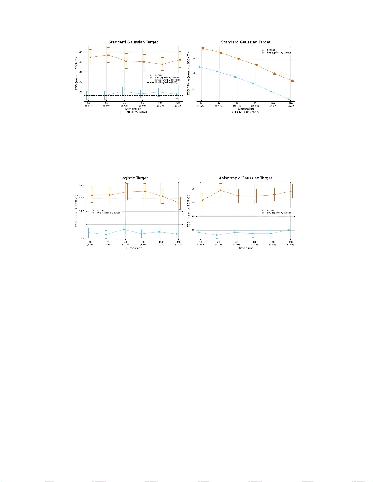
Submitted to the Annals of Applied Pr obability DIFFUSIVE SCALING LIMITS OF FOR W ARD EVENT -CHAIN MONTE CARLO: PR O V ABL Y EFFICIENT EXPLORA TION WITH P AR TIAL REFRESHMENT B Y H I RO F U M I S H I B A 1 , a A N D K E N G O K A M A TA N I 1 , b 1 Institute of Statistical Mathematics, a shiba.hir ofumi@ism.ac.jp ; b kamatani@ism.ac.jp Piecewise deterministic Markov process samplers are attractive alterna- tiv es to Metropolis–Hastings algorithms. A central design question is how to incorporate partial velocity refreshment to ensure ergodicity without in- jecting excessiv e noise. Forward Event-Chain Monte Carlo (FECMC) is a generalization of the Bouncy Particle Sampler (BPS) that addresses this is- sue through a stochastic reflection mechanism, thereby reducing reliance on global refreshment mov es. Despite promising empirical performance, its the- oretical efficienc y remains largely unexplored. W e dev elop a high-dimensional scaling analysis for standard Gaussian tar - gets and prove that the negati ve log-density (or potential) process of FECMC con verges to an Ornstein–Uhlenbeck diffusion, under the same scaling as BPS. W e deriv e closed-form expressions for the limiting diffusion coeffi- cients of both methods by analyzing their associated radial momentum pro- cesses and solving the corresponding Poisson equations. These expressions yield a sharp efficiency comparison: the diffusion coefficient of FECMC is strictly larger than that of optimally tuned BPS, and the optimum for FECMC is attained at zero global refreshment. Specifically , they imply an approx- imately eightfold increase in effecti ve sample size per event over optimal BPS. Numerical experiments confirm the predicted diffusion coef ficients and show that the resulting efficienc y g ains remain substantial for a range of non- Gaussian targets. Finally , as an application of these results, we propose an asymptotic variance estimator for Piecewise deterministic Markov processes that becomes increasingly efficient in high dimensions by extracting informa- tion from the velocity v ariable. 1. Introduction. Since the introduction of the random walk algorithm by Metropolis et al. ( 1953 ), Markov chain Monte Carlo (MCMC) methods hav e found widespread appli- cations in physics and statistics, particularly in Bayesian statistics following the advocacy of Gelfand and Smith ( 1990 ). While the Metropolis–Hastings (MH) paradigm introduced by Hastings ( 1970 ) has underpinned the majority of applications, a fundamentally different class of algorithms based on piecewise deterministic Markov processes (PDMPs) ( Davis , 1984 ) has emerged as a viable alternati ve. These methods originated in computational physics and molecular simulation as rejection-free, e vent-dri ven algorithms designed to ov ercome the dif fusi ve behavior inherent in MH-type dynamics ( Bernard, Krauth and W ilson , 2009 ; Pe- ters and de W ith , 2012 ; Michel, Kapfer and Krauth , 2014 ; F aulkner et al. , 2018 ; Krauth , 2021 ) and were later adopted in the statistical literature ( V anetti et al. , 2018 ; Bouchard-Côté, V ollmer and Doucet , 2018 ; Bierkens, Fearnhead and Roberts , 2019 ; Fearnhead et al. , 2018 ; Faulkner and Livingstone , 2024 ). Algorithms designed within the PDMP framework enjoy two key structural advantages that are typically lost in MH-based methods. First, PDMPs are inherently irreversible, and this lack of detailed balance has been shown to accelerate con- ver gence relativ e to rev ersible counterparts, a well-documented fact in both computational MSC2020 subject classifications : Primary 60F17; secondary 65C05, 65C40, 60J25. K e ywor ds and phrases: Piecewise deterministic Marko v processes, forward ev ent-chain Monte Carlo, bouncy particle sampler, high-dimensional scaling limits, output analysis. 1 2 physics ( Nishikawa et al. , 2015 ; Lei, Krauth and Maggs , 2019 ) and statistics ( Andrieu and Li vingstone , 2021 ; Eberle and Lörler , 2024 ). Second, and crucially for modern large-scale inference, the PDMP framework naturally accommodates unbiased subsampling and stochas- tic gradients while preserving the exactness of the target distribution ( Bierkens, Fearnhead and Roberts , 2019 ; Sen et al. , 2020 ; Fearnhead et al. , 2024 ). This stands in contrast to most stochastic gradient MH methods, which typically introduce asymptotic bias in exchange for scalability ( W elling and T eh , 2011 ; Chen, Fox and Guestrin , 2014 ; Nemeth and Fearnhead , 2021 ). Other structural benefits of PDMP-based samplers, including rob ustness in multiscale targets and bespoke implementation for special targets, are also under activ e in vestigation ( Bierkens et al. , 2023 ; Che vallier , Fearnhead and Sutton , 2023 ). Despite these adv antages, a precise understanding of the high-dimensional scaling behav- ior of PDMP-based samplers remains incomplete. In particular , although sev eral PDMP algo- rithms have been proposed, there is still no fully unified theoretical framework for comparing their ef ficiency or guiding practical algorithmic choices in high dimensions, despite the fact that scaling analysis is well established for MH-type methods; see Section 2.1 . In this work, we address this gap by deri ving high-dimensional dif fusi ve scaling limits, which enable a theoretical comparison of their computational complexity and asymptotic efficienc y . W e fo- cus on two representati ve and widely used methods: the Bouncy Particle Sampler (BPS) ( Bouchard-Côté, V ollmer and Doucet , 2018 ) and the Forw ard Event-Chain Monte Carlo (FECMC) ( Michel, Durmus and Sénécal , 2020 ). Both methods employ piecewise linear dy- namics perturbed by directional changes at random e vent times. A key difference is ho w randomness is injected via their directional changes: BPS employs deterministic reflections and thus relies on global refreshment mo ves for randomization, whereas FECMC achie ves it through a stochastic reflection mechanism. In BPS, there is a tension in selecting the Poisson rate ρ for the global refreshment ev ents. While global refreshment is essential for ergodicity , it may also inject additional noise that can hinder efficient exploration of the target distri- bution. Therefore, the primary design goal of FECMC was to discard the global refreshment while preserving ergodicity . This is achiev ed by stochastic reflection that combines (1) partial refreshment of the velocity component parallel to the gradient and (2) minimal randomiza- tion of the orthogonal component. The effecti veness of this strategy has been demonstrated through numerical experiments in Michel, Durmus and Sénécal ( 2020 ). Howe ver , a theoret- ical explanation for this observed improv ement is lacking. In particular , it remains unclear whether additional global refreshment ( ρ > 0 ) would accelerate e xploration. W e provide a theoretical explanation by directly comparing the high-dimensional diffusion scaling limits between FECMC and BPS. In Section 3 , we establish the weak con vergence theorems for the FECMC radial momentum process and the negati ve log-density (or po- tential) process. W e start with the case ρ = 0 , which requires new techniques. In this case, the FECMC process loses the regeneration structure on which the martingale arguments of Bierkens, Kamatani and Roberts ( 2022 ) crucially depend. By considering the dual predictable projection instead of the generator, we deriv e the limit theorem for the case of ρ = 0 through a semimartingale technique ( Méti vier , 1982 ; Jacod and Shiryaev , 2003 ). W e note that the case ρ = 0 has not been considered since BPS f ails to be er godic under this choice. Once the case ρ = 0 is understood, the extension to ρ > 0 follows naturally by combining our approach with the techniques de veloped in Bierkens, Kamatani and Roberts ( 2022 ) to analyze BPS. For the standard Gaussian targets, this limit turns out to be an Ornstein–Uhlenbeck (OU) process d Y t = − σ 2 ( ρ ) 4 Y t d t + σ ( ρ ) d B t , where only the diffusi vity parameter σ 2 dif fers between FECMC and BPS. Therefore, a com- parison of σ will enable us to compare the limiting speeds of the two processes and ultimately DIFFUSIVE SCALING LIMITS OF FECMC 3 the asymptotic efficienc y of the two algorithms. Howe ver , the pre vious expression for σ of BPS obtained in Bierk ens, Kamatani and Roberts ( 2022 ) inv olves an intractable inte gral, which hinders direct comparison. In Bierkens, Kamatani and Roberts ( 2022 ), the authors ap- proximated this quantity numerically and proposed using it to tune the refreshment rate ρ by maximizing diffusi vity σ 2 . In Section 4 , we deriv e explicit analytic formulae for the dif- fusion coefficients of both BPS and FECMC (Theorem 4.1 ). W e plot the result in Figure 1 , which illustrates the dominance of FECMC over BPS. This is achiev ed by reinterpreting the intractable inte gral as an expectation in v olving the associated resolvent operator of the radial momentum process and explicitly solving the associated Poisson equations. Interestingly , our results suggest that increasing σ 2 , and hence speeding up the limiting negati ve log-density process Y , can be achieved by improving the spectral properties of the radial momentum process. Consequently , we analytically establish that FECMC achiev es a higher speed than e ven a perfectly tuned BPS in sufficiently high dimensions. Additionally , we conclude that FECMC is most ef ficient when the refreshment rate ρ is set to zero, and any additional noise will only deteriorate performance. This confirms that the stochastic reflection mechanism of FECMC successfully preserves the necessary amount of randomization, thereby enabling ef- ficient exploration while remaining free of hyperparameter ρ and computationally cheaper . W e support our analysis and its robustness through numerical e xperiments in Section 5 . F I G 1 . Diffusion coefficient σ of the limiting negative log-density (potential) pr ocess vs. the global refr eshment rate ρ (FECMC vs. BPS). Standar d Gaussian target with spherical velocity . Curves computed from the analytic expr essions in Theorem 4.1 . Finally , our analysis implies no vel insights into PDMP output analysis. In practice, the velocity (or momentum) v ariable v is typically treated as a purely auxiliary component and is thus discarded after simulation. Howe ver , we argue that v may serve as a fast proxy for con vergence diagnosis when the mixing of x is too slow . Specifically , in our setting, the mixing time of the negativ e log-density U ( X t ) scales as O ( d ) , whereas its time deri v a- ti ve ( ∇ U ( X t ) | V t ) mixes on an O (1) timescale. This separation of timescales suggests that asymptotic variance estimation based on the time deriv ati ve can be more ef ficient in high dimensions than applying the same estimator directly to U . W e formalize this observ ation as a corollary to our main results in Section 4.3 and illustrate it empirically in Section 5.3 , focusing on the commonly used batch means estimator . 2. Background and Setting. 2.1. Diffusion Scaling Limits for MCMC Algorithms. In Monte Carlo applications, the dimension d of the state space can be very large, especially in modern data science and ma- chine learning. A central question is thus ho w the efficienc y of a gi ven algorithm scales with 4 d . In the statistics literature, the scaling analysis approach based on diffusion approximations was introduced in Roberts, Gelman and Gilks ( 1997 ) to analyze the high-dimensional be- havior of MCMC samplers. The authors deriv ed a weak conv ergence limit for finite dimen- sional projections of the random walk MH algorithm under appropriate time scaling. The limiting dif fusion process captures ef fecti ve first-order dynamics on a macroscopic scale. Since then, scaling analysis has been applied to algorithms beyond the random-walk MH algorithm ( Roberts, Gelman and Gilks , 1997 ; Mattingly , Pillai and Stuart , 2012 ), such as the Metropolis-adjusted Langevin algorithm ( Roberts and Rosenthal , 1998 ; Pillai, Stuart and Thiéry , 2012 ) and Hamiltonian Monte Carlo ( Beskos et al. , 2013 ). While the diffusion limit theorems for MH-type algorithms are highly advanced ( Roberts and Rosenthal , 2001 ; Sherlock et al. , 2015 ; Roberts and Rosenthal , 2016 ; Zanella, Bédard and K endall , 2017 ; Bierkens and Roberts , 2017 ; Kamatani , 2018 ; Kuntz, Ottobre and Stu- art , 2019 ; Kamatani , 2020 ; Y ang, Roberts and Rosenthal , 2020 ), those for PDMP algorithms are still limited. For the high-dimensional asymptotic re gime d → ∞ , there are only two works, to our knowledge, Deligiannidis et al. ( 2021 ) and Bierkens, Kamatani and Roberts ( 2022 ), that directly consider PDMPs. These two studies identified different limits, which stem from different choices of the velocity distrib ution µ d . In the work of Bierkens, Ka- matani and Roberts ( 2022 ), µ d is the uniform distribution on the unit sphere S d − 1 in R d , enabling a direct comparison between BPS and the Zig-Zag sampler (ZZS) ( Bierkens, Fearn- head and Roberts , 2019 ). W ith this choice µ d = Unif ( S d − 1 ) , the coordinate processes of BPS hav e been proven to possess OU limits under an O ( d ) time scaling. The authors also con- sidered the negati ve log-density process. For both processes, they concluded an O ( d 2 ) com- putational complexity to generate approximately independent samples. On the other hand, in Deligiannidis et al. ( 2021 ), µ d is set to the d -dimensional standard Gaussian distribution. Consequently , without time scaling, the finite dimensional coordinate processes of BPS hav e been prov en to con verge to the Randomized Hamiltonian Monte Carlo (RHMC) processes ( Bou-Rabee and Sanz-Serna , 2017 ). In this way , they were able to theoretically v alidate the O ( d 3 / 2 ) computational complexity for the one-dimensional marginal distribution observed in the numerical experiments of Bouchard-Côté, V ollmer and Doucet ( 2018 ). Howe ver , for the negati ve log-density process, the scaling dif fers and appears less fav orable than in the case µ d = Unif ( S d − 1 ) ; see Deligiannidis et al. ( 2021 ); Bierkens, Kamatani and Roberts ( 2022 ). In both cases, the negati ve log-density constitutes one of the slo west mixing quantities. For other PDMP scaling regimes, the authors of Bierkens, Kamatani and Roberts ( 2025 ) consider an anisotropic limit, where the covariance structure of a two-dimensional Gaussian distribution factorizes into tw o increasingly dif ferent length scales. In Agrawal, Bierkens and Roberts ( 2025 ), the authors consider the large sample limit n → ∞ to compare different subsampling schemes of ZZS. In Agrawal et al. ( 2025 ), a central aim is to in vestigate the fluid limit as the initial starting point moves infinitely away from the mode to quantify how quickly different PDMP samplers return to the high-density region. In doing so, they consider a family of targets of the form π ϵ ( x ) ∝ e − U ( x ) /ϵ for ϵ > 0 and study the limit of ϵ → 0 . In their analysis, under appropriate assumptions, FECMC and the closely related Coordinate Sampler ( W u and Robert , 2020 ) are proved to perform outstandingly better than the other methods, including BPS and ZZS, achie ving O (1) computational complexity in the limit. 2.2. Setting and Notation. In this w ork, we focus on the radial momentum and the ne ga- ti ve log-density processes. Our choice is motiv ated by the observation that the mixing of these two quantities poses a more difficult yet statistically relev ant challenge for PDMP samplers; see also T erenin and Thorngren ( 2018 ); Sherlock and Thiery ( 2021 ); Deligiannidis et al. ( 2021 ). Our setting is therefore more suitable for approaching the worst-case computational complexity of these algorithms in a way that is closely aligned with the L 2 -con vergence DIFFUSIVE SCALING LIMITS OF FECMC 5 rate results in Andrieu et al. ( 2021 ); Lu and W ang ( 2022a , b ) and the total variation con- ver gence results in Deligiannidis, Bouchard-Côté and Doucet ( 2019 ); Durmus, Guillin and Monmarché ( 2020 ); V asdekis and Roberts ( 2022 ); Roberts and Rosenthal ( 2023 ). W e set the velocity distribution µ d to be the uniform distribution on the unit sphere S d − 1 in R d , i.e., µ d = Unif ( S d − 1 ) , in order to match the analysis of BPS in Bierkens, Kamatani and Roberts ( 2022 ). This choice is also made in the experiments of Michel, Durmus and Sénécal ( 2020 ), presumably to enable direct comparison with the original ev ent-chain Monte Carlo algorithm of Bernard, Krauth and W ilson ( 2009 ); Michel, Kapfer and Krauth ( 2014 ). Throughout our theoretical analysis in Sections 3 and 4 , the target distribution π d is as- sumed to be the d -dimensional standard Gaussian distribution (2.1) π d ( x ) : = 1 (2 π ) d/ 2 exp  − U d ( x )  , U d ( x ) : = | x | 2 2 = x 2 1 + · · · + x 2 d 2 , where the ne gativ e log-density function U d ( x ) will also be called the potential function here- after . Observe that U d is a function of the radial distance | x | , and therefore π d is a spherically symmetric distribution. For such targets, the potential process captures mixing in the radial direction. Our proof framew ork applies to more general product-form distributions, and we expect the OU limits in Theorems 3.7 and 3.9 to remain valid under appropriate integrabil- ity conditions. W e do not pursue sharp sufficient conditions here. A systematic treatment of such conditions, as well as extensions to dependent targets, will be an interesting direction for future work, as the numerical experiments in Section 5.2 suggest that this diffusi ve limit may persist e ven under weak dependence. Instead, by taking adv antage of the Gaussianity , we obtain closed-form expressions for σ in Theorem 4.1 , which lead to a rigorous asymptotic ef ficiency ordering between FECMC and BPS. For general targets, the diffusion coefficient σ typically needs to be ev aluated numerically; see Section 5 for empirical estimates. 2.3. Piecewise Deterministic Monte Carlo. PDMPs form a class of continuous-time Marko v processes that complement dif fusion processes ( Davis , 1984 , 1993 ). Most PDMPs that appear in modern Monte Carlo methodology have linear dynamics between random e vents, and their e xtended generators take the form (2.2) Lf ( z ) = ( v |∇ x f ( z )) + λ ( z ) Z R d  f ( x, v ′ ) − f ( x, v )  Q ( z , d v ′ ) , z = ( x, v ) ∈ R d × R d , for test functions f in an appropriate domain D ( L ) . Here, ∇ x f = ( ∂ x 1 f , · · · , ∂ x d f ) ⊤ denotes the gradient with respect to x , λ : R 2 d → R + : = [0 , ∞ ) is a continuous function called the rate (or intensity) function, and Q : R 2 d × B ( R d ) → [0 , 1] is a Markov kernel describing the jumps. ( ·|· ) denotes the inner product throughout. T o turn the PDMP ( 2.2 ) into a Monte Carlo sampler targeting a probability density π defined on R d , a velocity distribution µ on R d must be specified first. Then, typically , the PDMP with the product target π ⊗ µ is simulated. There are many choices for λ and Q to ensure con vergence to π ⊗ µ . A common choice for the rate function is (2.3) λ ( x, v ) = ( v |∇ U ( x )) + + ρ, ( x, v ) ∈ R 2 d , ρ ≥ 0 , where U ( x ) = − log π ( x ) is the potential, ρ is called the r efr eshment rate , and the notation ( x ) + : = max( x, 0) stands for the non-negati ve part of a real number x . Paired with this rate function, the jump is typically gi ven by Q ( z , B ) = ( v |∇ U ( x )) + λ ( z ) Q V ( z , B ) + ρ λ ( z ) µ ( B ) , B ∈ B ( R d ) , 6 where Q V is called a velocity jump kernel . Note that this choice of Q only changes the velocity v , and PDMPs with such a kernel Q are called velocity-jump PDMPs ( Othmer , Dunbar and Alt , 1988 ; Monmarché et al. , 2020 ; Durmus, Guillin and Monmarché , 2021 ). For example, BPS employs a deterministic jump called r eflection , which is defined by Q V ( z , · ) = δ ϕ ( z ) , where δ v is a Delta measure with its point mass on v ∈ R d , and ϕ : R 2 d → R d is gi ven by (2.4) ϕ ( x, v ) = ( v − 2 v ∥ , ∇ U ( x )  = 0 , v , ∇ U ( x ) = 0 , where v ∥ : = ( n ( x ) | v ) n ( x ) denotes the projection of v onto n ( x ) : = ∇ U ( x ) / |∇ U ( x ) | , which is defined when ∇ U ( x )  = 0 . W e will introduce the FECMC jump kernel in the following subsection 2.4 . For other design strategies for λ and Q , consult Fearnhead et al. ( 2018 ); V anetti ( 2019 ); W u and Robert ( 2020 ). Notably , Bou-Rabee and Sanz-Serna ( 2017 ); Bierkens et al. ( 2020 ); Kleppe ( 2022 ) employs nonlinear dynamics as its deterministic flo w . Under the above setting, a general condition ensuring in v ariance has been deri ved in Michel, Durmus and Sénécal ( 2020 ), which we summarize in the follo wing proposition. P RO P O S I T I O N 2.1 . Assume that the potential U ( x ) is continuously differ entiable and C 1 c ( R d ) is a core of the generator L given in ( 2.2 ) . If for every C 1 -function f with compact support, (2.5) Z R d ( v |∇ U ( x )) + Qf ( x, v ) µ (d v ) = Z R d ( v |∇ U ( x )) − f ( x, v ) µ (d v ) , π -a.s. x ∈ R d , wher e ( x ) − : = min( x, 0) , then the pr oduct distribution π ⊗ µ is the in variant distribution of the PDMP corr esponding to the generator L . Note that inv ariance alone does not necessarily imply con ver gence. T o ensure ergodicity , BPS requires a positi ve refreshment rate ρ > 0 in ( 2.3 ); see Bouchard-Côté, V ollmer and Doucet ( 2018 ). Choosing ρ too large injects uninformati ve noise, increases computational ov erhead, and leads to random-walk behavior . FECMC w as proposed in Michel, Durmus and Sénécal ( 2020 ) to resolve this issue by employing a stochastic velocity jump Q V . This FECMC jump k ernel Q V enables the choice of ρ = 0 without losing its ergodicity and there- fore frees the algorithm from this hyperparameter . In the following subsection, we detail the design of Q V . 2.4. The FECMC Algorithm. For FECMC, the velocity distribution µ is assumed to be spherically symmetric. Consider an ev ent triggered at the point z = ( x, v ) . The FECMC jump kernel Q V operates on an orthogonal decomposition of v with respect to the gradient direction n ( x ) = ∇ U ( x ) / |∇ U ( x ) | at x v = v ∥ + v ⊥ , v ∥ : = ( v | n ( x )) n ( x ) , where we suppressed the dependence on x in the notation. The ne w velocity v new ∼ Q V ( z , · ) is also constructed as v new = v ∥ new + v ⊥ new , where the two components are specified in turn as follo ws. Step1 The component v ∥ new , the projection onto the gradient direction n ( x ) , is set by v ∥ new : = − w n ( x ) , where the length w = | v ∥ new | is completely refreshed from a distribution q ∥ . q ∥ is specified to ensure the in v ariance condition ( 2.5 ). Specifically , this density q ∥ needs to take the form of (2.6) q ∥ ( w ) ∝ w µ 1 ( w )1 [0 , ∞ ) ( w ) , w ∈ R , DIFFUSIVE SCALING LIMITS OF FECMC 7 where µ 1 is the marginal density of the first component of µ ( Michel, Durmus and Sénécal , 2020 ). Note that this component v ∥ new does not depend on the pre vious velocity v . Step2 The perpendicular component v ⊥ new is ‘switched’ by first randomly choosing an or- thogonal matrix A ∈ R d × d and then transforming the previous perpendicular component v ⊥ by Av ⊥ . After renormalization, v ⊥ new is specified as v ⊥ new = 1 √ 1 − w 2 Av ⊥ , A ∼ ν x , where ν x is a certain probability distribution defined on the space of orthogonal matrices. Se veral choices for the probability distribution ν x are considered in Michel, Durmus and Sénécal ( 2020 ). Among them, the naïve orthogonal switch performs consistently best in the reported numerical results. This approach constructs the matrix A by A : = I d − ( e 1 − e 2 )( e 1 − e 2 ) ⊤ , where I d is the d -dimensional identity matrix, and e 1 and e 2 consist of a pair of or- thogonal unit vectors chosen uniformly at random from the unit sphere in n ( x ) ⊥ : = { u ∈ R d | ( u | n ( x )) = 0 } . A hyperparameter p ∈ (0 , 1) can be further incorporated to control the frequency of switch- ing, for example, by using A with a probability of p and I d in the other cases. Consult Michel, Durmus and Sénécal ( 2020 , Section 3) for other choices for ν x and further implementation strategies. In our theoretical analysis, we do not specify ν x since the changes caused by ν x do not af fect the radial direction due to the spherical symmetry of the standard Gaussian distribu- tion. For the numerical experiments in Section 5 , howe ver , we use orthogonal switches with a probability p = 0 . 05 , following the practice of Michel, Durmus and Sénécal ( 2020 , Sec- tion 4). For our choice of µ d = Unif ( S d − 1 ) , the distribution q ∥ ,d defined in ( 2.6 ) reduces to (2.7) q ∥ ,d ( w ) = ( d − 1) w (1 − w 2 ) d − 3 2 1 (0 , 1) ( w ) , w ∈ R . The asymptotic properties of this distribution play a crucial role in establishing our limit theorems; hence, they are studied in Appendix B . 3. Scaling Analysis of FECMC. Throughout, we study the FECMC process Z d t = ( X d t , V d t ) under the follo wing assumption. A S S U M P T I O N 3.1 . Assume that Z d admits the pr oduct-form in variant distrib ution π d ⊗ µ d , wher e π d = N d (0 , I d ) is the d -dimensional standar d Gaussian distrib ution and µ d = Unif ( S d − 1 ) is the uniform distribution on the unit spher e S d − 1 ⊂ R d ; see also ( 2.1 ) . Additionally , we assume a stationary start: Z d 0 ∼ π d ⊗ µ d . Under the high-dimensional asymptotic re gime d → ∞ , we study the limiting behavior of the follo wing two processes: the r adial momentum pr ocess (3.1) R d t : = ( X d t | V d t ) = d X i =1 X d,i t V d,i t , t ≥ 0 , and the scaled potential pr ocess (3.2) Y d t : = 2 U d ( X d dt ) − d √ d = | X d dt | 2 √ d − √ d, t ≥ 0 . 8 Note that on the right-hand side of ( 3.2 ), X d is accelerated by a factor of O ( d ) to deriv e a non-degenerate scaling limit, while R d remains on the original scale. Both processes are hereafter viewed as random variables taking values in the Skorokhod space. As such, we first deri ve a PDMP scaling limit for R d , together with a fe w properties of this limit, in Section 3.1 . Observe that R d is the time deri v ative of Y d . This result is then used to establish the diffusion limit of Y d in Section 3.2 . Although both limiting processes, which we denote by Y and R , are Marko v , for any fixed d ≥ 1 , neither X d nor R d is Markov with respect to its natural filtration. This poses a major challenge in deri ving the limit theorems. This was partially resolved within a semimartingale frame work in the proof of Theorem 2.10 in Bierkens, Kamatani and Roberts ( 2022 ). Ho wever , the argument crucially relies on the regeneration structure in R d induced by global refreshment. Therefore, further techniques are required to address the case where global refreshment is absent, i.e., ρ = 0 . This issue is specific to FECMC. For BPS, the limit theorem does not hold when ρ = 0 due to the loss of ergodicity . W e outline a unifying framework that subsumes this boundary case in Section 3.3 , while deferring all proofs to the appendices. Appendix A contains the proof and the required auxiliary propositions for our main Theorem 3.7 . It uses results on the jump structure in Appendix B and the limit theorem for Y d in Appendix C . 3.1. Radial Momentum. The standard Rayleigh distrib ution (equi valently , the χ distribu- tion with two degrees of freedom), denoted by χ (2) , has the density xe − x 2 / 2 on x > 0 ; see, e.g., Forbes et al. ( 2010 , Chapter 39). P RO P O S I T I O N 3.2 (Limit of the Radial Momentum Process) . Suppose Assumption 3.1 holds and set the global r efreshment rate to zer o ( ρ = 0 ). As d → ∞ , the radial momentum pr ocess R d ( 3.1 ) con verg es weakly to a PDMP R F , whose (extended) g enerator L F is given by (3.3) L F f ( x ) = f ′ ( x ) + x +  E[ f ( − τ )] − f ( x )  , wher e x + : = min( x, 0) and the expectation is taken with respect to τ ∼ χ (2) , a standar d Rayleigh random variable . The superscript F stands for FECMC. A corresponding radial momentum process R B and a generator L B for BPS will be defined subsequently in Remark 3.8 . C O RO L L A RY 3.3 (Number of V elocity Jumps). The number of velocity jumps of Z d over a fixed time interval (0 , T ] satisfies E   X 0 ≤ t ≤ T 1 { ∆ V d t  =0 }   = T √ 2 π , T > 0 , for all d = 1 , 2 , · · · . R E M A R K 3.4 (Asymptotic Ratio of Mean Jump Frequencies) . In a typical implementa- tion of PDMP algorithms, the number of jumps appr oximately corresponds to the number of gradient evaluations. Thus, the number of jumps is widely used as a pr oxy for computational complexity; see Bierkens, F earnhead and Roberts ( 2019 ); Krauth ( 2021 ). F or FECMC, this quantity is asymptotically strictly smaller than that of BPS (cf. Cor ollary 2.9 of Bierkens, Kamatani and Roberts 2022 ), partly because the (optimal) FECMC pr ocess does not employ any global r efr eshment move (corresponding to ρ = 0 ). When the asymptotically optimal DIFFUSIVE SCALING LIMITS OF FECMC 9 choice ρ ∗ (see Theor em 4.1 below) is employed in BPS, the expected number of jumps for FECMC is appr oximately 1 √ 2 π 1 √ 2 π + ρ ∗ ≈ 0 . 218 · · · times that of BPS. R E M A R K 3.5 (Asymptotic Ratio of ESS per Event). Since the asymptotic variance of the er godic average of a FECMC trajectory is in versely pr oportional to σ 2 F (Theor em 4.1 ), the effective sample size (ESS) is pr oportional to σ 2 F . Combining this with the estimate σ 2 F /σ 2 B ( ρ ∗ ) ≈ 1 . 73 · · · in Remark 4.2 , the ESS per event under FECMC is appr oximately 1 . 73 / 0 . 218 = 7 . 93 · · · times larg er than that under BPS. In Section 5.1 , we additionally ob- serve an appr oximate fifteen-fold gap in ESS per CPU time. This additional widening is explained by the per-e vent costs. The global refr eshment move in BPS r equir es drawing a new d -dimensional velocity fr om µ d , followed by normalization. P RO P O S I T I O N 3.6 (Exponential Ergodicity of R F ) . Let γ denote the one-dimensional standar d Gaussian distribution. The limiting radial momentum pr ocess R F is γ -in variant and exponentially er godic. Specifically , ther e exists a function V ∈ L 1 ( γ ) and constants c 1 , c 2 > 0 such that ∥ P t ( x, − ) − γ ∥ TV ≤ c 1 e − c 2 t V ( x ) , t ≥ 0 , x ∈ R , wher e P t is the Markov tr ansition kernel associated with R F . 3.2. P otential. Now we formulate our main result, first for the case ρ = 0 . The case ρ > 0 is cov ered in Theorem 3.9 . T H E O R E M 3.7 (Scaling Limit of the Potential Process when ρ = 0 ) . Suppose Assump- tion 3.1 holds and set the global r efr eshment r ate to zer o ( ρ = 0 ). As d → ∞ , the scaled potential pr ocess Y d con verg es in law to an Ornstein–Uhlenbeck (OU) pr ocess that solves an SDE (3.4) d Y t = − σ 2 F 4 Y t d t + σ F d B t , wher e σ 2 F : = p 32 /π and ( B t ) t ≥ 0 is a one-dimensional standar d Br ownian motion. R E M A R K 3.8 (Comparison with BPS) . The functional form of ( 3.4 ) coincides with that of BPS, as reported in Theor em 2.10 of Bierkens, Kamatani and Roberts ( 2022 ). The only differ ence is that the coefficient σ 2 F is r eplaced by (3.5) σ 2 B ( ρ ) : = 8 Z ∞ 0 e − ρt K B ( t, 0) d t, ρ > 0 , wher e K B is the covariance function of the BPS limiting radial momentum pr ocess R B . The gener ator L B associated with R B r eads (3.6) L B f ( x ) = f ′ ( x ) + x +  f ( − x ) − f ( x )  . Ther efore , the limiting pr ocess of FECMC is a time-c hanged version of BPS’ s limiting poten- tial pr ocess thr ough t 7→ ( σ 2 F /σ 2 B ( ρ )) t . F or the optimal choice ρ ∗ for BPS, the Monte Carlo 10 estimate reported in Bierkens, Kamatani and Roberts ( 2022 ) gives σ 2 F /σ 2 B ( ρ ) ≈ 1 . 77 , indi- cating that the limiting FECMC potential dynamics ar e faster than those of BPS. Another appr oach for comparison may be formulated in terms of the speed measur e, as in Roberts, Gelman and Gilks ( 1997 ), which can be defined for a br oader class of diffusions ( Revuz and Y or , 1999 , Section VII.3). F or OU pr ocesses, the speed measur e is in versely pr oportional to the drift coefficient. Note that the pr ocess is faster when the speed measur e is smaller . More- over , t 7→ σ 2 F t, σ 2 B t ar e the quadratic variations of these limiting pr ocesses. Larg er values of σ F , σ B ar e ther efor e favorable also fr om the vie wpoint of quadr atic variation, a continuous- time analogue for expected squar ed jump distance (ESJD) in discrete-time settings ( Sherlock , 2006 ; Sherlock and Roberts , 2009 ; Besk os et al. , 2013 ). T o facilitate a rigorous comparison of σ F and σ B , we introduce the positi ve global refresh- ment rate ρ > 0 into FECMC, making σ F a function of ρ > 0 , as is the case with the BPS dif fusion coefficient σ B in ( 3.5 ). FECMC with global refreshment ( ρ > 0 ) is contrary to the recommendation of Michel, Durmus and Sénécal ( 2020 ). Our purpose here is twofold: (1) to theoretically confirm that the choice ρ = 0 is indeed optimal for FECMC, and (2) to establish analytically that σ B ( ρ ) < σ F holds for all ρ > 0 , which will be carried out in Section 4 . T H E O R E M 3.9 (Scaling Limit of the Potential Process when ρ > 0 ) . Suppose Assump- tion 3.1 holds and the global r efr eshment rate is positive ( ρ > 0 ). As d → ∞ , the scaled potential pr ocess of FECMC con verg es in law to the OU pr ocess that solves the SDE ( 3.4 ) with σ F r eplaced by (3.7) σ 2 F ( ρ ) : = 8 Z ∞ 0 e − ρt K F ( t, 0) d t wher e K F is the covariance function of the FECMC limiting r adial momentum pr ocess R F . R E M A R K 3.10 (Continuity at ρ = 0 ) . One might e xpect that Theor em 3.7 should be cov- er ed by taking the limit ρ ↘ 0 , i.e., σ 2 F ( ρ ) → σ 2 F . However , this con verg ence turns out to be very delicate. W e establish this r esult in Cor ollary 4.3 below . By contrast, for BPS, this limit as ρ → 0 turns out to be zer o, r eflecting the failur e of the limit theor em. The abov e theorem is closely related to Theorem 2.10 in Bierkens, Kamatani and Roberts ( 2022 ), which states a corresponding result for BPS. The argument in Bierkens, Kamatani and Roberts ( 2022 ) relies on the regeneration structure induced by the global refreshment, combined with careful control of residual terms using Stein’ s method. Howe ver , Theorem 3.7 cannot be handled by the same approach and requires new techniques. W e discuss our ap- proach to addressing this in the follo wing subsection. 3.3. Pr oof Strate gy . A classical approach to weak con ver gence results such as Propo- sition 3.2 and Theorems 3.7 , 3.9 is to apply a T rotter–Kato type theorem, in which con- ver gence is derived from the associated Markov semigroups or generators; see, e.g., T rotter ( 1958 ); Y oshida ( 1995 ). Howe ver , in our setting, the processes R d and Y d are not Marko v with respect to their natural filtrations. There are primarily two approaches to deriv e scaling limits for such non-Markovian processes. Let A 1 , A 2 , · · · be a sequence of such processes. One approach is to embed A d into a proper Mark ov process A d on an augmented state space and vie w A d as its projection. W ithin the general framework of Section 4.8 in Ethier and Kurtz ( 1986 ), a suitable notion of generator con vergence for A d yields weak conv er gence of the marginal processes A d to wards a possibly non-Marko vian limiting process. Many of the previous works employ this strategy; see, e.g., Roberts, Gelman and Gilks ( 1997 ); DIFFUSIVE SCALING LIMITS OF FECMC 11 Roberts and Rosenthal ( 1998 ); Bierkens and Roberts ( 2017 ); Y ang, Roberts and Rosenthal ( 2020 ); Agrawal et al. ( 2023 ) for applications of this approach. In doing so, one typically needs homogenization-type results in adv ance, such as Lemma 2.1 in Roberts, Gelman and Gilks ( 1997 ), to v erify the required generator con ver gence. In our case, ho wev er , the relev ant homogenization-type result for limiting coefficients is obtained only after the limit theorem has been established (Corollary 4.3 ). This difference essentially arises from our choice of subject: we study the potential process instead of the finite-dimensional marginal coordinate processes, as in Roberts, Gelman and Gilks ( 1997 ). Because the potential process is an ad- diti ve functional, its dif fusi vity is a time integral in v olving the corresponding time-deriv ative process, known as the Green–Kubo formula; see Equation ( 4.2 ). Establishing that this quan- tity is finite, howe v er , is generally delicate. A natural route is to derive an estimate for the resolvent operator ( λ − L ) − 1 as λ ↘ 0 , associated with the generator L , in the spirit of the Kipnis–V aradhan program ( Kipnis and V aradhan , 1986 ), but this can be technically demand- ing; see also Section 6 . W e therefore adopt a second approach to establish scaling limit theorems for the potential process and the radial momentum process. This approach yields a cleaner separation between the probabilistic deriv ation of the limit and the subsequent analytic reinterpretation. W e vie w A d as a semimartingale and work with its predictable characteristics; see Jacod and Shiryaev ( 2003 , Definition II.2.6) and Métivier ( 1982 , Definition 32.2) for a precise definition. The semimartingale characteristics are a triplet that can be regarded as a probabilistic generaliza- tion of the generator of a Marko v process, as they determine the distribution of a semimartin- gale under suitable conditions. T o establish con ver gence, we prove that the characteristics con verge in an appropriate sense within the framew ork of Jacod and Shiryaev ( 2003 , Chap- ter IX). PDMPs are particularly well suited for this semimartingale approach because their underlying point process structure naturally gi ves rise to semimartingale decompositions. This strategy has been applied to PDMPs in Bierkens, Kamatani and Roberts ( 2022 ) and to MH-based methods in Kamatani ( 2018 , 2020 ), and is closely related to martingale CL T ap- proaches to function space MCMC methods ( Mattingly , Pillai and Stuart , 2012 ; Pillai, Stuart and Thiéry , 2012 , 2014 ; Ottobre et al. , 2016 ). 4. Diffusivity of FECMC and BPS. In this section, we deriv e analytic expressions for the diffusion coefficient σ 2 F , σ 2 B , which appeared in our limit theorems in Equations ( 3.7 ) and ( 3.5 ) respecti vely . Perhaps surprisingly , the resulting formulae obtained in Theorem 4.1 are very explicit, being rational functions of the moment generating function of the standard Rayleigh distribution; see Section 4.1 . The values of σ 2 F and σ 2 B computed from Theorem 4.1 are plotted as functions of ρ > 0 in Figure 1 . As illustrated in Figure 1 , these representations enable a rigorous comparison of asymptotic ef ficiency between FECMC and BPS. Addition- ally , we can conclude that any global refreshment introduced by setting ρ > 0 will slo w do wn the limiting process and thus deteriorate the efficienc y of FECMC; see Section 4.2 . All proofs are deferred to Appendix D . 4.1. Analytic F ormulae for Diffusion Coefficients. σ 2 F and σ 2 B turn out to be determined solely through associated radial momentum processes R F , R B . Although the corresponding two generators L F and L B dif fer only in one term, the mixing properties of R F associated with L F are significantly improv ed ov er those of R B . T o see this, we focus on the function (4.1) f F ( x ; ρ ) : = Z ∞ 0 e − ρt E[ R F t | R F 0 = x ] d t = ( ρ − L F ) − 1 id( x ) , ρ > 0 , where id( x ) = x is the identity function. f B is defined analogously for BPS. The in verse operator ( ρ − L F ) − 1 that appears on the right-hand side of ( 4.1 ) is called the resolvent as- sociated with the generator L F , and it is well-defined for each ρ > 0 ; see Ethier and Kurtz 12 ( 1986 , Proposition 2.1 p.10) or Engel and Nagel ( 2000 , Theorem II.1.10). Using this function f F , the dif fusion coef ficient σ F is expressed as (4.2) σ 2 F ( ρ ) 8 = Z ∞ 0 e − ρt E[ R F 0 R F t ] d t = E  R F 0 f ( R F 0 ; ρ )  , ρ > 0 . The first equality is simply a re writing of ( 3.7 ) and expresses the diffusion coefficient as an integrated autocorrelation function; it is known as the Green–K ubo formula ( Kubo, T oda and Hashitsume , 1991 ; Pa vliotis , 2010 ). The second equality holds due to Fubini’ s theorem after taking the conditional expectation. Consequently , using Equation ( 4.2 ), we will obtain explicit formulae for σ F and σ B by solving the resolvent equation ( 4.1 ) for f F . The result turns out to be a rational function of the moment generating function of the standard Rayleigh distribution. Before stating the results, we introduce the follo wing notation: (4.3) Ω( ρ ) : = r π 2 ρ erfcx  ρ √ 2  = ρe ρ 2 2 Z ∞ ρ e − t 2 2 d t, where erfcx( x ) = 2 e x 2 √ π R ∞ x e − t 2 d t is the e xponentially scaled complementary err or function ; see Cody ( 1969 ); Oldham, Myland and Spanier ( 2009 ). This Ω is related to the moment generating function through the relationship E[ e ρτ ] = 1 − Ω( − ρ ) , where τ ∼ χ (2) ; see Ap- pendix D . More importantly , this function Ω is numerically stable and was used to produce Figure 1 , thereby av oiding numerical overflo ws due to scale differences. T H E O R E M 4.1 (Formulae for σ F , σ B ) . Under the same assumptions as Theor em 3.9 , (4.4) σ 2 F ( ρ ) = σ 2 F  1 −  ρ 2 − ρ p π 2 + Ω( ρ )  2 ρ 4 Ω( ρ )(2 − Ω( ρ ))  , wher e σ 2 F = p 32 /π , and (4.5) σ 2 B ( ρ ) = 8 ρ 4 ρ 3 − ρ 2 r 8 π + ρ − r 8 π  (1 + ρ 2 )Ω( ρ ) − ρ 2  2 Ω(2 ρ ) ! . R E M A R K 4.2 (Optimizing the Obtained Expression) . Now that we have analytic expr es- sions, we are able to numerically optimize σ 2 B , for example, using the algorithm of Brent ( 1971 ). This function attains its maximum value σ 2 B ( ρ ∗ ) = 1 . 838 · · · at ρ ∗ = 1 . 423 · · · . This is strictly smaller than σ 2 F = p 32 /π ≈ 3 . 19 · · · . These values will be compar ed to the re- sults of numerical experiments in Section 5 . In particular , we will observe that the ratio σ 2 F /σ 2 B ( ρ ∗ ) ≈ 1 . 73 · · · is fairly r ob ust to the assumptions and is valid under various targ et distributions other than the standar d Gaussian distributions. 4.2. Optimal Global Refr eshment Rate for FECMC. In general, establishing the con ver - gence of this quantity as ρ ↘ 0 is delicate; see K omoro wski, Landim and Olla ( 2012 ). How- e ver , giv en the analytic formulae in Theorem 4.1 , we can conclude that the inte gral con ver ges and recov er the v alue predicted by Theorem 3.7 . C O RO L L A RY 4.3 (Continuity at ρ = 0 ) . As ρ ↘ 0 , we have σ 2 F ( ρ ) → σ 2 F = r 32 π , σ 2 B ( ρ ) → 0 . Next, we prov e that the function σ 2 F is maximized at ρ = 0 , thereby confirming that the design goal of Michel, Durmus and Sénécal ( 2020 ) is met. This is also evident from Figure 1 . DIFFUSIVE SCALING LIMITS OF FECMC 13 C O RO L L A RY 4.4 (Monotonicity of σ 2 F ) . d σ 2 F ( ρ ) d ρ < 0 , ρ > 0 . 4.3. A F ast Pr oxy for Asymptotic V ariance Estimation in High Dimensions. In Section 3 , we showed that the potential process Y d admits a non-degenerate limit only after scaling time by a factor d , whereas the radial momentum process R d has a stable limit on the orig- inal timescale. In other words, the mixing of the potential becomes increasingly slow as d gro ws, while R d does not. This separation of timescales is also reflected in the efficienc y of asymptotic v ariance estimation for ergodic a verages. W e consider two test functions that correspond to Y d and R d , namely the scaled negati ve log-density and its time deri v ati ve: (4.6) h ( x ) : = U ( x ) − E π [ U ( X )] p V ar π [ U ( X )] , g ( x, v ) : = ( v |∇ U ( x )) − E π ⊗ µ [( V |∇ U ( X ))] p V ar π ⊗ µ [( V |∇ U ( X ))] . By construction, h and g hav e zero mean and unit variance under the stationary distribution. Consequently , it suffices to study the estimation of E π [ h ( X )] and E π ⊗ µ [ g ( X , V )] , both of which are zero. For the standard Gaussian tar get, each function simplifies to: h ( x ) = 1 √ 2 | x | 2 − d √ d , g ( x, v ) = ( x | v ) . In Section 5 , we estimate their means using the ergodic a verages (4.7) b h d T : = 1 T Z T 0 h ( X d s ) d s, b g d T : = 1 T Z T 0 g ( X d s , V d s ) d s. The following proposition provides the v alues of the asymptotic variances of b h d T and b g d T , respecti vely . The proof is giv en in Appendix D . P RO P O S I T I O N 4.5 (Asymptotic V ariance F ormulae). Under Assumption 3.1 , lim T →∞ lim d →∞ T V ar[ b h d dT ] = 8 σ 2 F , lim T →∞ lim d →∞ T V ar[ b g d T ] = σ 2 F 4 . Note that, for h d , we evaluate the time average over a horizon of length dT to pr oduce non- de generate variance, matc hing the diffusive time scaling of Y d in Section 3 . Proposition 4.5 suggests a fast proxy for the asymptotic v ariance estimation of b h d . A com- mon approach is to apply a batch means (BM) estimator constructed from time a verages of h ov er successi ve short time intervals called batches; see Flegal and Jones ( 2010 ); Liu, V ats and Flegal ( 2022 ) and also Bierkens, Fearnhead and Roberts ( 2019 ) for application to PDMPs. Since the correlation time of h ( X d t ) grows on the O ( d ) timescale, stable BM estimation for h requires the batch size to scale at least on the order of d ; see the dT time horizon for b h d in Proposition 4.5 . In contrast, the same proposition indicates that σ 2 F can also be inferred from b g d , which uses only a time horizon on the order of O (1) . In this way , one may estimate σ 2 F , and thus the asymptotic variance for h , using roughly 1 /d of the computational budget. This reciprocal relationship is deriv ed from the property of the OU limit and is observed to persist be yond the standard Gaussian target. W e empirically demonstrate the ef fectiveness of this approach for dif ferent targets in Section 5.3 . This BM estimator via the fast proxy g equals the unbiased sample variance of the ener gy increments ov er batches, i.e., U d ( X d t i ) − U d ( X d t i − 1 ) . This value is computationally cheaper 14 than the standard BM estimator for h , since computing b h d T generally requires integrating h ( X d t ) along the trajectory via numerical quadrature. Howe ver , there is a pitfall in applying our fast proxy trick. Note that changing the order of the limits yields lim d →∞ lim T →∞ T V ar[ b g d T ] = 0 . This reflects the fact that the asymptotic variance of the ergodic av erage ˆ g d T is zero, an im- mediate fact that follows from the telescoping property . Therefore, our proposed estimator dif fers fundamentally from the usual application of a BM-type estimator , which would yield a trivial estimator . W e will demonstrate that an appropriate choice of batch size will indeed lead to an efficient estimator for σ 2 F in Section 5.3 . The appropriate batch size appears to be much smaller than usual practice ( Liu, V ats and Flegal , 2022 ); see Section 5.3 . Identifying appropriate regimes in which our estimator has consistency , as well as a systematic treatment beyond the standard Gaussian tar gets, will be a practically important future direction. Our estimator is closely related in spirit to Einstein–Helfand-type estimators for transport coef ficients in molecular dynamics (MD) ( Helfand , 1960 ; V iscardy , Servantie and Gaspard , 2007 ). Asymptotic variance estimation of ergodic a verages is also very important in Bayesian inference, especially in MCMC output analysis and the development of adaptiv e versions of the algorithm. In the former , asymptotic variance estimators are utilized to assess conv er- gence and sample quality ( Jones et al. , 2006 ; Flegal and Gong , 2015 ; Gong and Flegal , 2016 ), report Monte Carlo standard errors (MCSEs) ( Flegal, Haran and Jones , 2008 ), and construct confidence regions for posterior estimates ( Atchadé , 2016 ; Robertson et al. , 2021 ); see V ats et al. ( 2020 ); Roy ( 2020 ) for further details. In the latter , the estimator of the asymptotic v ariance (or proxies thereof) is optimized internally to tune algorithmic parameters on the fly ( Andrieu and Robert , 2001 ; Pasarica and Gelman , 2010 ; W ang et al. , 2025 ). 5. Experiment. In this section, we v alidate our theory by first probing dimensional- ity scaling in Section 5.1 and then checking robustness to the Gaussian assumption in Sec- tion 5.2 . W e mainly consider the mean estimation of the function h , as well as g in Sec- tion 5.3 . Both of them are defined in ( 4.6 ). While our theory has focused on the diffusion coef ficients σ F , σ B , we mainly report the effecti ve sample size (ESS) in this section for the sake of interpretability . W e define the ESS for h as ESS( h ) = T /ς 2 h , where T is the time hori- zon and ς 2 h is the asymptotic variance of the ergodic average b h T , which is defined in ( 4.7 ). Recall that the v ariance of h under stationarity is 1 by construction. Both samplers are initialized in stationarity . The refreshment rate ρ of BPS is set to 1.42, the asymptotically optimal choice; see Remark 4.2 and Bierkens, Kamatani and Roberts ( 2022 ). F or FECMC, an orthogonal switch is performed approximately e very fifty e vents (i.e., p = 0 . 05 ), follo wing the practice in Michel, Durmus and Sénécal ( 2020 ). Both algo- rithms share the same implementation that uses the automated Poisson thinning technique of Andral and Kamatani ( 2024 ). W e implement only the direction change step separately , keeping the rest of the code identical for a fair comparison. The code is av ailable in the Supplementary Material ( Shiba , 2026 ). 5.1. Dimensionality Scaling: FECMC vs. BPS. W e vary the dimension from d = 10 to d = 320 and compare the values predicted by our theory with experimental values. W e con- sider the same test function h defined in ( 4.6 ). When both algorithms are run ov er the time interv al [0 , dT ] , Proposition 4.5 predicts that the ESSs should be independent of d , and for the standard Gaussian targets, the v alues should be (5.1) ESS FECMC ( h ) = T σ 2 F 8 = T √ 2 π ≈ 39 . 8 , ESS BPS ( h ) = T σ 2 B ( ρ ∗ ) 8 ≈ 22 . 9 , DIFFUSIVE SCALING LIMITS OF FECMC 15 respecti vely; see Remark 4.2 . W e set T = 100 . W e construct an estimator for the mean squared errors (MSEs) of h by av eraging the squared errors of the empirical av erages over R = 1000 independent runs: [ MSE T : = 1 R R X r =1  1 dT Z dT 0 h ( X r t ) d t  2 , h ( x ) = U ( x ) − V ar π [ U ] p V ar π [ U ] . Finally , we report the estimated ESS calculated by d ESS T = 1 / [ MSE T , together w ith its asso- ciated BCa bootstrap confidence interv al. W e consider three different targets π 1 , π 2 , π 3 : (1) the standard Gaussian π 1 , (2) the multi- v ariate standard logistic distrib ution π 2 ( x ) = Q d i =1 e x i (1+ e x i ) 2 , and (3) an anisotropic Gaussian π 3 ∝ exp( − x ⊤ Σ − 1 x/ 2) , where Σ ii = 1 and Σ ij = γ for i  = j . For the third target, we set γ = 1 / 2 in this section; other choices are explored in the ne xt subsection. First, for the standard Gaussian target π 1 , we confirm that the ESSs of both FECMC and BPS are independent of the dimension d and closely match the theoretical v alues, with all the 95% confidence interv als cov ering the theoretical values; see the left panel of Figure 2 . In particular, our theory provides a very good approximation e ven in moderate dimensions, such as d = 10 and 20 . When computational cost is tak en into account, the difference in performance becomes more pronounced; see the right panel of Figure 2 . This is because FECMC requires fewer e vent simulations; see Remark 3.4 . The estimated ESS per CPU second amounts to approximately a fifteen-fold dif ference. The in verse linear dependence on dimensionality reflects the O ( d ) scaling of the time horizon. For the second experiment, the multi variate logistic distribution π 2 presents two addi- tional challenges: heavier tails and a lack of spherical symmetry , while remaining isotropic across the coordinates. W e observe that these departures from isotropic Gaussianity do not substantially alter the ov erall behavior , except for a reduction in the ESSs for both FECMC and BPS; see the left panel of Figure 3 . Ho we ver , although the absolute values of ESS have changed, the ESS ratio between FECMC and BPS still remains close to the theoretical value σ 2 F /σ 2 B ( ρ ∗ ) ≈ 1 . 73 · · · , which is deriv ed under the standard Gaussian assumption; see Re- mark 4.2 In the third experiment, the samplers are confronted with strong anisotropy induced by correlations among the coordinates. Once again, we observe behavior similar to that of the standard Gaussian case; see the right panel of Figure 3 . Ho we ver , there are some notable de viations. First, the ESSs are slightly increased, which may be explained by a reduction in the intrinsic dimension caused by the correlation structure. Second, the ESS ratio is larger than that of the isotropic case. In the ne xt section, we will observe that this relati ve efficiency gain widens as the le vel of anisotropy increases. W e will discuss possible explanations there. Overall, these e xperiments confirm the rele vance of our high-dimensional analysis to ev en moderate dimensions and support the robustness of both the theoretical scaling predictions and the efficienc y ratio prediction σ 2 F /σ 2 B ( ρ ∗ ) ≈ 1 . 73 · · · across a range of targets with in- creasing structural complexity . 5.2. Robustness to De viations fr om Isotr opic Gaussianity . Fixing d = 100 , we per- form two experiments that introduce progressiv ely stronger deviations from isotropy and Gaussianity , respecti vely . In the first e xperiment, we re visit the anisotropic Gaussian set- ting π 3 ( x ) ∝ exp( − x ⊤ Σ − 1 x/ 2) and vary the off-diagonal entries of the covariance matrix: Σ ij = γ ∈ { 0 , 0 . 1 , 0 . 2 , · · · , 0 . 9 } for i  = j . In the second experiment, we consider the spheri- cally symmetric Student distribution π 4 ( x ) ∝ (1 + | x | 2 /ν ) − ( d + ν ) / 2 with varying degrees of freedom ν ∈ { 10 , 10 2 , 10 3 , 10 4 } ; see Fang, K otz and Ng ( 1990 ) for details on this distribu- tion. Although the Student distrib ution has polynomial tails for any finite ν ≥ 1 , it con ver ges 16 F I G 2 . Estimated ESS (Left) and ESS per CPU second (Right), together with 95% BCa bootstrap confidence intervals, against dimensionality . The parenthesized values below the x -ticks r epr esent the ESS mean ratio of FECMC to BPS at each dimension. The estimator is given by d ESS T = 1 / [ MSE T for T = 100 . Both plots ar e based on 1000 independent runs of BPS and FECMC, targ eting the standard Gaussian distribution π 1 ( x ) ∝ exp( −| x | 2 / 2) . The two black lines in the left plot repr esent the theoretical limiting values ( 5.1 ) when d, T → ∞ for FECMC and BPS r espectively . F I G 3 . Estimated ESS against dimensionality , together with 95% BCa bootstrap confidence intervals. The tar get distribution is either the i.i.d. logistic distribution π 2 ( x ) = Q d i =1 e x i (1+ e x i ) 2 (left plot) or the anisotropic Gaussian distribution π 3 ∝ exp( − x ⊤ Σ − 1 x/ 2) , where Σ ii = 1 and Σ ij = 0 . 5 for i  = j (right plot). In both cases, each algorithm is run 1000 times independently with the time horizon T = 100 . to the standard Gaussian distribution as ν → ∞ , thereby capturing varying degrees of tail heaviness. W e will call the v alue of ν − 1 tail heaviness. The results are summarized in Figure 4 . The left edge in both plots corresponds to the Gaussian, or approximately Gaussian, target, where our theoretical predictions (indicated by dotted black lines) are within the 95% confidence intervals. Ho we ver , we also see that both experiments probe a broad spectrum of de viations from the standard Gaussian set- ting, including regimes in which the theoretical assumptions are substantially violated on the right edge. While a clear departure from the theoretical predictions is observ ed at ex- treme parameter values, the theory remains remarkably robust for moderate deviations, with both the ESS and the ESS ratio closely matching the predicted values. Interestingly , in the anisotropic Gaussian experiment (left panel of Figure 4 ), when the correlation is v ery strong, such as γ = 0 . 9 , FECMC significantly outperforms BPS, amounting to a 3.6-fold gap in ESS. This phenomenon may w arrant further in vestigation, particularly under alternati ve scaling regimes, such as those considered in Beskos et al. ( 2018 ); Au, Graham and Thiery ( 2023 ). W e hypothesize that this phenomenon is due to the irrev ersible nature of the fluid limit, in the sense of Fort et al. ( 2008 ); Agrawal et al. ( 2025 ), of the one-dimensional linear projec- DIFFUSIVE SCALING LIMITS OF FECMC 17 tion FECMC process, which cannot be observed for BPS ( Bierkens, Kamatani and Roberts , 2022 ). F I G 4 . Estimated ESS against deviation parameters γ , ν − 1 , which quantify departures fr om isotropy and Gaus- sianity , together with 95% BCa bootstrap confidence intervals. The tar get distribution is either the anisotropic Gaussian π 3 ( x ) ∝ exp( − x ⊤ Σ − 1 x/ 2) with varying correlations Σ ij = γ ∈ { 0 , 0 . 1 , 0 . 2 , · · · , 0 . 9 } (left plot) or the spherically symmetric Student distribution π 4 ( x ) ∝ (1 + | x | 2 /ν ) − ( d + ν ) / 2 with varying degr ees of fr eedom ν ∈ { 10 , 10 2 , 10 3 , 10 4 } (right plot). The blac k lines denote theor etical limiting values derived under the standar d Gaussian assumption in Eq. ( 5.1 ) In both cases, the dimension is d = 100 and each algorithm is run 1000 times independently with the time horizon T = 100 . 5.3. A F ast Pr oxy for Asymptotic V ariance Estimation. In practice, the asymptotic vari- ance of ergodic av erages is estimated from a single trajectory , as it can be computationally expensi ve to run the algorithm se veral times independently . This estimate can also be aggre- gated among multiple chains to diagnose con vergence ( V ats and Knudson , 2021 ). A common choice for this task is the batch means (BM) estimator . For the test function h and computa- tional horizon T , it is giv en by: b ς 2 h = 1 B − 1 B X i =1 ( Y i − Y ) 2 , Y i : = 1 √ b Z ib ( i − 1) b h ( X t ) d t, where Y is the sample mean of { Y i } B i =1 , and b = T /B is the batch size; see also Section 2 in the supplement of Bierk ens, Fearnhead and Roberts ( 2019 ). This estimator is consistent as T → ∞ under appropriate conditions ( Flegal and Jones , 2010 ). Howe ver , this estimator has a notoriously se vere bias-variance trade-off within a finite computational budget; therefore, v ariance reduction methods are acti vely pursued ( Flegal and Jones , 2010 ; V ats and Flegal , 2021 ; Liu, V ats and Flegal , 2022 ). In Section 4.3 , we proposed a fast proxy trick: the time deri vati ve of h can yield a more ef- ficient estimator for the asymptotic variance of b h . In this section, we empirically demonstrate that the BM estimator associated with g , denoted by b ς 2 g , can be more efficient in terms of MSE than b ς 2 h in high dimensions. W e consider two target distributions from Section 5.1 ; the standard Gaussian distribution π 1 and the anisotropic Gaussian distribution π 3 with γ = 1 / 2 . Both BM estimators are constructed over the time interval [0 , T d ] , where T = 10 4 . For the batch size of b ς 2 h , we employ the asymptotically optimal choice in terms of MSE, which is deri ved explicitly in Liu, V ats and Flegal ( 2022 ). For b ς 2 g , we set b/ (10 4 √ d ) = 1 . 5 , 2 , respec- ti vely . This choice can be suboptimal; optimal batch size selection for our proposed estimator will be an important topic for future research. W e report the values of (5.2) b ς 2 slow := b ς 2 h , b ς 2 fast := 2 / b ς 2 g , 18 respecti vely . They are both estimators for the asymptotic variance ς 2 h of the ergodic average ˆ h . This v alue equals ς 2 h = 8 /σ 2 F = √ 2 π for the standard Gaussian target π 1 . For the anisotropic Gaussian target π 3 , we use the estimated asymptotic variances in Section 5.1 as a proxy for the true v alues of b ς 2 slow and b ς 2 fast to compute MSE. Figure 5 shows boxplots of b ς 2 slow and b ς 2 fast ov er 100 independent runs, together with the MSE of each estimator . F or both targets, we observe that b ς 2 slow has stable variation across all dimensions, whereas both the variance and the bias of b ς 2 fast decrease as the dimension grows. As a result, the MSE ordering rev erses, with b ς 2 fast e ventually outperforming b ς 2 slow , and the adv antage widens as d becomes large. F I G 5 . Boxplots of two estimators, b ς 2 slow and b ς 2 fast , over 100 runs against incr easing dimensions d . The tar gets ar e either the standard Gaussian distribution π 1 ( x ) ∝ exp( −| x | 2 / 2) (left plot) or the anisotropic Gaussian distribution π 3 ( x ) ∝ exp( − x ⊤ Σ − 1 x/ 2) with Σ ii = 1 and Σ ij = 0 . 5 for i  = j (right plot). The black lines in both plots r epr esent the (pr oxy of) true values. The subplot on the bottom repr esents the mean squared err or (MSE) of each estimator . Our experiment suggests that using b ς 2 g instead of the usual BM estimator b ς 2 h results in a lo wer MSE when the dimension d is large, and that this phenomenon can be observed for a wide variety of targets other than standard Gaussian distributions. As b g T is easy to compute on the fly , it may be used to design an adaptive PDMP scheme ( Bertazzi and Bierkens , 2022 ) by maximizing the estimate internally ( W ang et al. , 2025 ). Adaptive estimation of transport coef ficients, such as σ F in our context, has also been considered in molecular dynamics ( Jones and Mandadapu , 2012 ). 6. Conclusion. T o facilitate the development of ev en more efficient PDMP algorithms, we hav e proposed analyzing the potential process Y , as it constitutes one of the slowest quan- tities in typical PDMP dynamics. Through its time deri vati ve process R , we ha ve established the diffusi ve scaling limits in Section 3 . Our proof techniques were crucial in establishing the limit for ρ = 0 , the most interesting case for FECMC. The dimensionality scaling O ( d ) turns out to be identical to BPS. Subsequently , in Section 4 , we provided closed-form formulae for the dif fusion coefficients σ F and σ B . Our e xplicit representations were made possible by explicitly solving the Poisson equation − L − 1 f = id , where L is the generator of R . This dif- fusion coef ficient turns out to depend solely on the solution f . This observ ation can f acilitate potential improvements in existing PDMP samplers. For instance, maximizing the value, or the e xpectation ( 4.2 ), of this solution f within the state-dependent speed function framework of Bertazzi and V asdekis ( 2025 ) will improve the mixing of the potential process. Addition- ally , we suggested using the variance of squared increments as a proxy for estimating the asymptotic variance of the ergodic av erages of the potential. This exploits the fine structure DIFFUSIVE SCALING LIMITS OF FECMC 19 that resides in the continuous-time trajectory and is unique to PDMP samplers. Its effecti ve- ness in high dimensions was explained theoretically as an application of our scaling analysis results and demonstrated numerically . The fast proxy estimator b ς 2 fast , defined in Eq. ( 5.2 ), lev erages the variability of the veloc- ity variable by using finer batching than standard batch means estimators. The relationship that 2 / b ς 2 g matches b ς 2 slow is a consequence of the OU limit. Accordingly , our estimator relies crucially on the existence of an OU limit for the rescaled potential process. Our experiments suggest this OU limit holds quite universally , thereby supporting the effecti veness of the pro- posed estimator for the potential function. A more systematic treatment is in order; ho wev er , we lea ve it for future w ork. This estimator is closely related to variance reduction techniques based on control variates. In this context, the functions f F and f B in Eq. ( 4.2 ) can be seen as a continuous analogue of the fishy function defined and discussed in Douc et al. ( 2025 ); South and Sutton ( 2025 ). As mentioned in discussing our proof strategy in Section 3.3 , our limit theorems are closely related to the Kipnis–V aradhan approach to CL Ts for additiv e functionals of Markov pro- cesses, initiated in Kipnis and V aradhan ( 1986 ). In that setting, a centered additi ve functional A t : = Z t 0 V ( X s ) d s of an ergodic Marko v process ( X t ) t ≥ 0 is considered. In our case, X corresponds to the limit- ing radial momentum process R . With this choice, A coincides with the potential process Y by taking V ( x ) = x . Howe ver , our approach differs in two ways from that of Kipnis and V aradhan ( 1986 ) and from subsequent extensions to irre versible processes such as Bhat- tacharya ( 1982 ); Cattiaux, Chafai and Guillin ( 2011 ); K omorowski, Landim and Olla ( 2012 ). First, the primary interest in these works is the scaling limit of a single process of the form α − 1 d A dt for a suitable space-scaling function d 7→ α d , whereas we study a sequence of pro- cesses ( A d ) ∞ d =1 as we take the limit d → ∞ . In other words, we are simultaneously con- sidering a high-dimensional limit and a scaling limit as d → ∞ . Second, our dev elopment proceeds in the reverse order of the Kipnis–V aradhan program. In typical Kipnis–V aradhan- type arguments, one starts from analytic assumptions ensuring that the resolvent ( ρ − L ) − 1 behav es well as ρ ↘ 0 , and then deduces a (functional) central limit theorem together with a Green–Kubo-type formula for the asymptotic variance. In contrast, we first identify the lim- iting process and its diffusion coef ficient in Theorems 3.7 and 3.9 , and only afterwards show that the limit ρ ↘ 0 indeed provides the asymptotic v ariance (Theorem 4.1 ). APPENDIX A: CONVERGENCE OF THE PO TENTIAL The objectiv e here is to prov e Theorem 3.7 , deri ving the limit of the potential processes Y d as d → ∞ . Recall that Z d = ( X d , V d ) is the output of FECMC on R d , a Marko v process by design. Howe ver , Y d is not a Markov process with respect to its natural filtration ( F d t ) , e ven though it is Mark ov with respect to the filtration ( G d t ) generated by Z d . A.1. Con vergence of the Piecewise Constant Appr oximations. T o prove the con ver- gence of Y d , we first prov e the con vergence of its skeleton processes Y d , which are defined belo w in ( A.1 ), composed of the points Y d S n /d on the e vent times S n rescaled by a factor of d − 1 . After this, we finalize the proof by establishing asymptotic equi valence between Y d and Y d . The jump times of the FECMC process Z d are denoted by 0 = S 0 , S 1 , S 2 , · · · , which are ( G t ) -stopping times. Note that the y are ( F d t ) -stopping times as well, as long as ( F d t ) is right- continuous, which we assure ourselves here. Using these stopping times ( S n ) , we define the 20 skeleton pr ocess Y d by (A.1) Y d t : = ∞ X n =0 Y d S n /d 1 [ S n d , S n +1 d ) ( t ) . W e now deri ve its dual predictable projection. W e first define F d n : = F d S n /d − , which is the σ -field of events strictly prior to the jump at S n /d . Substituting n with n ( t ) : = max { n ≥ 0 | S n ≤ dt } , we consider the continuous-time filtration ( F d n ( t ) ) . W ith respect to this filtration, the dual predictable projection of Y d is gi ven by (A.2) B d t : = ∞ X n =1 E h ∆ Y d n    F d n ( t ) − 1 i 1 [ S n − 1 d , ∞ ) ( t ) , where ∆ Y d n : = Y d S n /d − Y d S n − 1 /d . See, e.g., Méti vier ( 1982 , 15.7) and Jacod and Shiryae v ( 2003 , II.3.11). This predictable projection B d constitutes one of the local characteristics, or the triplet, of the semimartingale Y d . The other two are the (predictable) quadratic v ariation C d = ⟨ M d,c ⟩ of the continuous part of M d : = Y d − B d − Y d 0 and the dual predictable projection ν d of the random measure associated with the jumps of Y d . These three characteristics B d , C d , ν d are respectiv ely called the first, second, and third characteristic. For general definitions, see Méti vier ( 1982 , 32.2) and Jacod and Shiryaev ( 2003 , II.2.6). W e first derive the limits of the characteristics ( B d , C d , ν d ) and establish Theorem 3.7 based on the frame work of Jacod and Shiryae v ( 2003 , Theorem IX.3.48). A.1.1. Con verg ence of the F irst Characteristic. W e start with the first characteristic B d . From now on, we will often add the superscript of d in the stopping time S n as S d n to indicate its ambient dimension, as its distributional properties crucially depend on d . W e introduce the notation T d n : = S d n − S d n − 1 . P RO P O S I T I O N A.1 (Con ver gence of the first characteristic B d ) . Defining b ( y ) = − q 2 π y , it holds for all N ≥ 1 that sup 1 ≤ n ≤ N d      Z S d n /d 0 b ( Y d t ) d t − n X i =1 E[∆ Y d i |F d i − 1 ]      P − − − → d →∞ 0 , N ≥ 1 . P RO O F . T o re write the statement, let us define the follo wing two processes: (A.3) ∆ M d n : = − S d n d − S d n − 1 d ! r 2 π Y d S d n − 1 d − E[∆ Y d n |F d n − 1 ] , M d n : = n X i =1 ∆ M d i = − n X i =1 S d i d − S d i − 1 d ! r 2 π Y d S d i − 1 d − n X i =1 E[∆ Y d i |F d i − 1 ] . The statement is now equiv alent to the conv ergence sup 1 ≤ n ≤ N d | M d n | → 0 in probability for an arbitrary N ≥ 1 . As discussed in Section 3.3 , one major obstacle in proving this con ver - gence is that M d is only asymptotically martingale. Howe ver , we can employ the following generalized Doob inequality ( Méti vier , 1982 , Corollary 9.7) (A.4) ϵ 2 P " sup 1 ≤ n ≤ N d | M d n | > ϵ # ≤ | λ d 2 | ((0 , N d ] × Ω) + E h | M d N d | 2 i , DIFFUSIVE SCALING LIMITS OF FECMC 21 where ϵ > 0 , N ≥ 1 and λ d p are the Doléans-Dade measure of the quasimartingale | M d n | p for p ≥ 1 ; see, e.g., Métivier ( 1982 , 8.6). This inequality will reduce our proof to the con ver gence of the first and second moments of M d n . W e confirm this by treating the two terms in the right-hand side of ( A.4 ) one by one. The first term can be bounded as follo ws: | λ d 2 | ((0 , N d ] × Ω) = N d X n =1 λ d 2 (( n − 1 , n ] × Ω) = N d X n =1 E      E[( M d n ) 2 |F d n − 1 ] − ( M d n − 1 ) 2      = N d X n =1 E      E[(∆ M d n ) 2 |F d n − 1 ] + 2 M d n − 1 E[∆ M d n |F d n − 1 ]      ≤ N d X n =1 E[(∆ M d n ) 2 ] + 2 N d X n =1 E  | M d n − 1 |     E[∆ M d n |F d n − 1 ]      . According to Lemma A.2 that follows, we have | λ d 2 | ((0 , N d ] × Ω) d →∞ − − − → 0 if we can show that E[ | M d N d | 2 ] → 0 . This fact follows immediately from Lemma A.2 and the follo wing rela- tionship: E[ M 2 N d ] = N d X i =1 E[(∆ M d n ) 2 ] + 2 X i>j E[∆ M d i ∆ M d j ] . L E M M A A.2 . The following asymptotic evaluations hold for ∆ M d n defined in ( A.3 ) E[∆ M d n |F d n − 1 ] = O P ( d − 3 2 ) , E[(∆ M d n ) 2 |F d n − 1 ] = O P ( d − 2 ) , ( d → ∞ ) . P RO O F . The proof is straightforward once the asymptotic e xpressions of T d i and ∆ Y d i are gi ven in Lemma B.3 and B.4 , respecti vely . The calculation proceeds as follo ws: E[∆ M n |F d n − 1 ] = E " − r 2 π S d n d − S d n − 1 d ! Y d S d n − 1 /d − E[∆ Y d n |F d n − 1 ]      F d n − 1 # = − r 2 π Y d S d n − 1 /d E[ T d n |F d n − 1 ] d − E[∆ Y d n |F d n − 1 ] = − r 2 π Y d S d n − 1 /d  √ 2 π d + O P ( d − 3 2 )  + 2 d + 1 Y d S d n − 1 /d + O ( d − 3 2 ) = Y d S d n − 1 /d  2 d + 1 − 2 d  + O P ( d − 3 2 ) . The first term in the right-hand side is of order O P ( d − 2 ) . This implies the first equation in the statement. The second equation can be deduced similarly E[(∆ M d n ) 2 |F d n − 1 ] = E   S d n − S d n − 1 d ! 2 2 π ( Y d S d n − 1 /d ) 2     F d n − 1   22 + E " S d n − S d n − 1 d r 2 π Y d S d n − 1 /d E[∆ Y d n |F d n − 1 ]     F d n − 1 # + E[∆ Y d n |F d n − 1 ] 2 = E[( T d n ) 2 |F d n − 1 ] d 2 2 π ( Y d S d n − 1 /d ) 2 + E[ T d n |F d n − 1 ] d r 2 π Y d S d n − 1 /d E[∆ Y d n |F d n − 1 ] + E[∆ Y d n |F d n − 1 ] 2 . This time, all terms appearing on the rightmost side are of order O P ( d − 2 ) , gi ven lemmas B.3 and B.4 . A.1.2. Con verg ence of the Modified Second Characteristic. Here, we consider a modi- fied second characteristic e C d : = ⟨ M d ⟩ . This can be simplified as: e C d t : = ∞ X n =1  E[(∆ Y d n ) 2 |F d n − 1 ] − (E[∆ Y d n |F d n − 1 ]) 2  1 [ S n − 1 d , ∞ ) ( t ) . Since this quantity con verges to the second characteristic of the limiting process, which is the squared dif fusion coef ficient σ 2 F of the OU process ( 3.4 ) in our case. P RO P O S I T I O N A.3 (Con vergence of the Modified Second Characteristic B d ) . Setting c : = 8 √ 2 π , we have the following con verg ence: Z S d N d /d 0 c d t − N d X n =1  E[(∆ Y d n ) 2 |F d n − 1 ] − (E[∆ Y d n |F d n − 1 ]) 2  P − − − → d →∞ 0 . P RO O F . Reformulating the statement using ∆ N d n : = c T d n d −  E[(∆ Y d n ) 2 |F d n − 1 ] − (E[∆ Y d n |F d n − 1 ]) 2  , what we need to prove is exactly P N d n =1 ∆ N d n P − → 0 . Since (E[∆ Y d n |F d n − 1 ]) 2 = O P ( d − 2 ) from Lemma B.4 , we obtain E[(∆ N d n ) 2 ] = c 2 d 2 E[( T d n ) 2 ] − 2 c d E  T n E[(∆ Y d n ) 2 |F d n − 1 ]  + O ( d − 3 ) . Therefore, we obtain E[(∆ N d n ) 2 ] = O ( d − 2 ) from, again, Lemma B.4 . Consequently , we are able to finish the proof by the Marko v inequality P "      N d X n =1 ∆ N d n      > ϵ # ≤ N d X n =1 E[(∆ N d n ) 2 ] ϵ 2 d →∞ − − − → 0 for e very ϵ > 0 . A.1.3. F inalization. W e are in a position to finalize the proof by establishing the conv er- gence of the skeleton process Y d . P RO P O S I T I O N A.4 (Conv ergence of the skeleton processes) . The skeleton pr ocess Y d , defined in ( A.1 ) , con verg es in law to Y , as stated in Theor em 3.7 . DIFFUSIVE SCALING LIMITS OF FECMC 23 P RO O F . The con ver gence will be established within the frame work of Jacod and Shiryae v ( 2003 , Theorem IX.3.48). There are six conditions (i)-(vi) to be checked. b ( y ) = − ( p 2 /π ) y and c = p 32 /π , which appeared in Propositions A.1 and A.3 , respectiv ely , are the first and second characteristic of the limiting OU process Y , defined in ( 3.4 ). This fact leav es us with only two conditions, (v) and (vi), to be checked. Condition (v) is trivially satisfied from our stationarity assumption. Regarding condition (vi), given Propositions A.1 and A.3 , we only need to check the con vergence of the third characteristic ν d . This reduces to proving (A.5) dN X n =1 P[ | ∆ Y d S n | > ϵ ] d →∞ − − − → 0 for e very ϵ > 0 . This condition ( A.5 ) ensures condition 3.49 of Jacod and Shiryaev ( 2003 , Theorem IX.3.48) and also condition [ δ loc - D ] because there exists a choice of C 1 ( R ) ⊂ C b ( R ) such that, for ev ery g ∈ C 1 ( R ) , there exists a number L > 0 satisfying g ([ − L, L ]) = { 0 } and 0 ≤ g ( x ) ≤ 1 ( x ∈ R ) ; see Jacod and Shiryae v ( 2003 , III.2.7). F or such a function g , we hav e g ∗ ν d t = n ( t ) X n =1 g (∆ Y d S n ) ≤ n ( t ) X n =1 1 n | ∆ Y d S n | >L o ∴ P[ g ∗ ν d t ] ≤ n ( t ) X n =1 P[ | ∆ Y d S n | > L ] , where n ( t ) = max { n ≥ 0 | S n ≤ dt } . T aking large enough N > 0 , we can assume n ( t ) ≤ N d with a high probability from Corollary 3.3 . By considering the ev ent { n ( t ) > N d } sep- arately , it remains to prove ( A.5 ), as in the proof of Bierkens, Kamatani and Roberts ( 2022 , Theorem 2.10). This fact, ho we ver , immediately follows from the moment estimate E[ | ∆ Y d S n | 3 ] = O ( d − 3 / 2 ) implied by Lemma B.4 and Mark ov’ s inequality for p = 3 . A.2. Asymptotic Equivalence of the Appr oximation. W e finalize the proof of Theo- rem 3.7 by proving the asymptotic equiv alence of Y d and Y d . The following condition en- sures that Y d and Y d share the same limit; see Jacod and Shiryae v ( 2003 , Lemma VI.3.31). P RO P O S I T I O N A.5 (Asymptotic equiv alence of Y d and Y d ) . F or every positive r eal number T > 0 , sup 0 ≤ t ≤ T | Y d t − Y d t | P − − − → d →∞ 0 . P RO O F . The difference between Y d and Y d in each time interval t ∈ [ S n /d, S n +1 /d ] can be bounded as | Y d t − Y d S n /d | = 1 √ d     | X d td | 2 − | X d S n | 2     ≤ 2 √ d Z S n +1 S n | R d s | d s = 2 √ d  | R d S n | T n +1 + T 2 n +1 2  , where the rightmost side no longer depends on the time t . Given that Y d t − Y d t = ∞ X n =0  Y d S n /d − Y d t  1 [ S n d , S n +1 d ) ( t ) , we are able to bound, for e very ϵ > 0 as P  sup 0 ≤ t ≤ T | Y d t − Y d t | > ϵ  ≤ P[ n ( T ) > N d ] + P " N d [ n =0 ( sup t ∈ [ S n /d,S n +1 /d ] | Y d t − Y d S n /d | > ϵ )# ≤ P[ n ( T ) > N d ] + N d X n =0 P h d − 1 / 2  2 | R d S n | T n +1 + T 2 n +1  > ϵ i , 24 where n ( t ) = max { n ≥ 0 | S n ≤ dt } . In the right-hand side, the first term con verges as d → ∞ from Corollary 3.3 and Markov’ s inequality for p = 1 . The second term also con verges by Markov’ s inequality for p = 3 and the fact that R d S n and T n +1 hav e bounded absolute moments of any order , conditioned on F d S n /d − ; see Equations ( B.1 ) and ( B.2 ) in Section B.2 and the proof of Lemma B.1 . A.3. Proof of Theorem 3.9 . No w that Theorem 3.7 is established, Theorem 3.9 can be established along the same lines as in the proof of Theorem 2.10 in Bierkens, Kamatani and Roberts ( 2022 ), combined with results in Section B ; hence, we omit the details. APPENDIX B: ASYMPTO TICS OF A UXILIAR Y QU ANTITIES This section collects se veral lemmas concerning the asymptotic properties of certain (con- ditional) distributions related to the jumps of the FECMC process Z d . The results are hea vily used in Section A . B.1. Refreshment Distribution. The distribution q ∥ ,d , introduced in ( 2.7 ), arises as the length distribution of a refreshed radial component of the velocity V d S n at a jump time S n . W e need moment estimates to deri ve further properties concerning jumps of Z d . L E M M A B.1 (Asymptotic Properties of the New Radial V elocity). F or the random vari- able W d with a pr obability density q ∥ ,d , it holds that E[ W d ] = 1 2 B  1 2 , d + 1 2  = r π 2 d − 1 2 + O ( d − 1 ) ( d → ∞ ) , E[( W d ) 2 ] = 2 d + 1 , E[( W d ) 4 ] = 8 ( d + 1)( d + 3) , E[( W d ) 6 ] = 48 ( d + 1)( d + 3)( d + 5) , wher e B is the beta function B ( z , w ) = R 1 0 t z − 1 (1 − t ) w − 1 d t . P RO O F . Integrating the density q ∥ ,d ( v ) , we obtain a simple e xpression for the correspond- ing distribution function F ∥ ,d ( v ) = 1 − (1 − v 2 ) d − 1 2 . Therefore, the second, fourth, and sixth moments can be computed from the fact that, for a uniform random v ariable U on [0 , 1] , ( F ∥ ,d ) − 1 ( U ) = q 1 − (1 − U ) 2 d − 1 d = W , kno wn as the in verse function method. Hence, given E[ U k ] = ( k + 1) − 1 ( k = 0 , 1 , 2 , · · · ) , we obtain E[( W d ) 2 ] = 1 − E[ U 2 d − 1 ] = 1 − 1 2 d − 1 + 1 = 2 d + 1 , E[( W d ) 4 ] = 1 − 2 E[(1 − U ) 2 d − 1 ] + E[(1 − U ) 4 d − 1 ] = 8 ( d + 1)( d + 3) , E[( W d ) 6 ] = 1 − 3 E[(1 − U ) 2 d − 1 ] + 3 E[(1 − U ) 4 d − 1 ] − E[(1 − U ) 6 d − 1 ] = 48 ( d + 1)( d + 3)( d + 5) . DIFFUSIVE SCALING LIMITS OF FECMC 25 For the mean of W d , a direct calculation re veals E[ W d ] = Z 1 0 xq ∥ ,d ( x ) d x = − Z 1 0 x  (1 − x 2 ) d − 1 2  ′ d x = Z 1 0 (1 − x 2 ) d − 1 2 d x = 1 2 B  1 2 , d + 1 2  = √ π 2 Γ  d +1 2  Γ  d 2 + 1  . The result follo ws from an asymptotic result regarding the ratio of two Gamma function v alues Γ( z + α ) Γ( z + β ) = z α − β  1 + ( α − β )( α + β − 1) 2 z + O ( | z | − 2 )  , ( | z | → ∞ ) , which follo ws from Stirling’ s series, as presented in T ricomi and Erdélyi ( 1951 ). P RO P O S I T I O N B.2 (Con ver gence to the Standard Rayleigh Distribution). The law of √ dW d con verg es in total variation to χ (2) . P RO O F . The density of √ dW d is q ∥ ,d ( y / √ d ) / √ d . This con ver ges to q ∥ ,d ( y / √ d ) √ d = ( d − 1) x  1 − x 2 d  d − 3 2 1 (0 , 1)  x √ d  d →∞ − − − → xe − x 2 2 1 (0 , ∞ ) ( x ) for all x ∈ R . B.2. Moments of Jump Intervals. W e calculate the first and second conditional mo- ments of the jump intervals T n +1 : = S n +1 − S n , giv en the v alue of X S n (or equiv alently Y S n /d ). This jump arri v al time T n +1 is determined as follo ws. Observe first that the FECMC rate, substituting ρ = 0 and U ( x ) = U d ( x ) = | x | 2 / 2 in ( 2.3 ), equals the positiv e part of R d t = ( X d t | V d t ) , the radial momentum ( 3.1 ). Note that the time deriv ativ e of R d t is constant 1 between jumps, as in our case | V d t | ≡ 1 . Therefore, R d t is again a piecewise deterministic process. When a jump occurs, a ne w position is determined as (B.1) R d S n d = −| X d S n − | W d , n = 1 , 2 , · · · , where W d is the random variable, independent of X d S n − , with a density q ∥ ,d . W e calculated the moments of W d in Lemma B.1 . Conditioned on S n and X d S n − , no jump occurs between t ∈ [ S n , S n + | X d S n − | W d ] as ( R d t ) + = 0 on this time interval. Once t > S n + | X d S n − | W d holds, R d t becomes positi ve, so a jump may occur with intensity R d t . Ov erall, the distribution of T n +1 can be represented by (B.2) T n +1 d = | X d S n − | W d + τ , where the random variable τ ∼ χ (2) , independent of X d S n − and W d , follo ws a Rayleigh distribution with the scale parameter 1 , satisfying (B.3) E[ τ ] = r π 2 , E[ τ 2 ] = 2 , E[ τ 4 ] = 8 , E[ τ 6 ] = 64 . L E M M A B.3 (Moments of Jump Intervals). Conditioned on the filtr ation ( F d t ) generated by Y d , we have E[ T n |F d S n − 1 /d − ] = √ 2 π + O P ( d − 1 2 ) , ( d → ∞ ) , E[ T 2 n |F d S n − 1 /d − ] = 4 + π + O P ( d − 1 2 ) , ( d → ∞ ) . 26 P RO O F . As Y d S n − 1 /d − = y corresponds to | X d S n − 1 | 2 = y √ d + d by definition ( 3.2 ), substi- tuting this into ( B.2 ) results in E[ T n | Y d S n − 1 /d − = y ] = E[ W d ] q y √ d + d + E[ τ ] = r π 2 r y √ d + 1 + O ( d − 1 2 ) + r π 2 , where we used Lemma B.1 and Equation ( B.3 ). The first equation follo ws immediately , giv en Y d S n − 1 /d − = O P (1) as d → ∞ for all n ≥ 1 . Similarly , the second statement follows from that E[ T 2 n | Y d S n − 1 /d − = y ] =  y √ d + 1  d E[( W d ) 2 ] + 2 E[ W d τ ] q y √ d + d + E[ τ 2 ] =  y √ d + 1  2 · d d + 1 + 2  π 2 + O ( d − 1 2 )  + 2 . B.3. Moments of Skeleton Increments. In Section A.1 , the dual predictable projection B d of the skeleton process Y d is proved to be a jump process with increments E[∆ Y d n |F d n − 1 ] , whose properties we are going to in vestigate. W e first observe that the radial momentum R d is the time deri v ati ve of the potential process U d ( X d t ) = | X d t | 2 / 2 . Using this, we hav e ∆ Y d n = Y d S n /d − Y d S n − 1 /d = 1 √ d  | X d S n | 2 − | X d S n − 1 | 2  = 1 √ d Z S n S n − 1 2 R d t d t = 2 √ d  R d S n − 1 T n + T 2 n 2  . Observe that the quantities R d t , T n appearing in the rightmost expression hav e already been studied in Equation ( B.1 ) and Lemma B.3 respecti vely . L E M M A B.4 (Moments of Skeleton Increments) . E[∆ Y d n |F d S n − 1 /d − ] = − 2 d + 1 Y d S n − 1 d − + O P ( d − 3 2 ) ( d → ∞ ) , E[(∆ Y d n ) 2 |F d S n − 1 /d − ] = 8 d + O P ( d − 3 2 ) , ( d → ∞ ) , E[(∆ Y d n ) 3 |F d S n − 1 /d − ] = 16 d 3 / 2 + O P ( d − 2 ) , ( d → ∞ ) . P RO O F . W e first express ∆ Y d n by R d S n − 1 and T n . Then substitute ( B.1 ) and ( B.2 ) within the expectation E y [ · ] : = E[ ·| Y d S n − 1 /d − = y ] to obtain ∆ Y d n = 1 √ d  − | X d S n − 1 | 2 ( W d ) 2 + τ 2  . W e can proceed as E y [∆ Y d n ] = − 1 √ d E[( W d ) 2 ] E y [ | X d S n − 1 | 2 ] + 1 √ d E[ τ 2 ] = − 1 √ d 2 d + 1 ( y √ d + d ) + 2 √ d = − 2 d + 1 y + 2 √ d 1 d + 1 , DIFFUSIVE SCALING LIMITS OF FECMC 27 where we used the fact that W d and τ are independent, the moment estimates of Lemma B.1 and ( B.3 ), and that E[ | X d S n | 2 | Y d S n /d − = y ] = y √ d + d. For the second result, we proceed similarly , E y [(∆ Y d n ) 2 ] = E y [ | X d S n − 1 | 4 ( W d ) 4 ] d − 2 d E y [ | X 2 S n − 1 | ( W d ) 2 τ 2 ] + E[ τ 4 ] d = 8 d d 2 ( d + 1)( d + 3)  1 + y √ d  2 − 8 d + 1  1 + y √ d  + 8 d . Lastly , we ha ve E y [(∆ Y d n ) 3 ] = 1 d 3 / 2 E y   −| X d S n − 1 | 2 ( W d ) 2 + τ 2  3  = d − 3 2  − E[( W d ) 6 ]( y √ d + d ) 3 + 3 E[( W d ) 4 ] E[ τ 2 ]( y √ d + d ) 2 − 3 E[( W d ) 2 ] E[ τ 4 ]( y √ d + d ) + E[ τ 6 ]  = d − 3 2  − 48 + 48 − 48 + 64 + O P ( d − 1 / 2 )  . APPENDIX C: CONVERGENCE OF THE RADIAL MOMENTUM The proof proceeds along the same lines as in Section A . Ho wev er , this time R d possesses a special structure. By focusing on the jump measure µ d and its dual predictable projection e µ d , first introduced by Jacod ( 1975 ), we are able to obtain much simpler proofs. C.1. Con vergence of the Third Characteristic. Let ( M d t ) t ≥ 0 be a time-homogeneous Poisson point process on ( R + ) 3 with its intensity measure giv en by ℓ ⊗ 2 + ⊗ q ∥ ,d ( v ) d v , where ℓ + is the Lebesgue measure on R + . The radial momentum process R d can be expressed as a stochastic integral with respect to M d : (C.1) R d t = R d 0 + t + Z (0 ,t ] × ( R + ) 2 1 [0 ,R d s − ] ( λ )( −| X d s | v − R d s − ) M d (d s d λ d v ) . This integral representation immediately provides us with the canonical semimartingale de- composition; in fact, it is a Doob–Meyer decomposition since R d is also a quasimartingale. This can be written as R d t = P R d t + M d t , where P R d t : = t − Z t 0 | X d s | √ d E[ √ dW d ]( R d s − ) + d s − Z t 0 ( R d s − ) 2 d s is the dual predictable projection of R d . Here, W d is a random variable with density q ∥ ,d ; see Lemma B.1 . A ke y observ ation in analyzing R d is that its jump measure µ d , defined by µ d (d t d u ) : = X s ∈ R + 1 { ∆ R d s  =0 } δ ( s, ∆ X s ) (d t d u ) 28 has the dual predictable projection e µ d with respect to the natural filtration of R d , defined by (C.2) e µ d (d t d u ) : = Z R 2 + 1 [0 ,R d s − ] ( λ ) δ { −| X d s | v − R d s − } (d u )d t d λq ∥ ,d ( v ) d v . W e can express the first characteristic P R d and the modified second characteristic ⟨ M d ⟩ solely through the third characteristic e µ d and test functions f ( u ) = u, u 2 : u ∗ e µ d t = Z t 0 u e µ d (d s d u ) = P R d t − t, (C.3) u 2 ∗ e µ d t = Z t 0 u 2 e µ d (d s d u ) = ⟨ M d ⟩ t . (C.4) Here, ∗ denotes integration with respect to a random measure, as in Jacod and Shiryaev ( 2003 , Section II.1). Therefore, the con ver gence of the local characteristics can be deriv ed simultaneously from the following lemma. Overall, Proposition 3.2 essentially follows from the con vergence of the jump distrib ution, i.e., Proposition B.2 . L E M M A C.1 (Strong Conv ergence of the Third Characteristic) . Let e µ t denote the third char acteristic of the limiting pr ocess R F in Pr oposition 3.2 . Then, the con ver gence sup 0 ≤ t ≤ T | f ∗ e µ d t − f ∗ e µ t ◦ R d | P − − − → d →∞ 0 holds for any Lipschitz continuous function f and f ( u ) = u p with p = 1 , 2 , · · · . Her e, the underlying pr obability space is the Sk or okhod space Ω : = D ( R ) , and R d , R F ar e consider ed to be maps Ω → Ω ; hence, a composition oper ator ◦ is well-defined. P RO O F . The limiting process R F defined in Proposition 3.2 also has an inte gral represen- tation: R t = R 0 + t + Z (0 ,t ] × R 2 + 1 [0 ,R s − ] ( λ )( − v − R s − ) M (d s d λ d v ) , where M is the Poisson random measure with intensity measure ℓ ⊗ 2 + ⊗ χ (2) . Observe that the third characteristic satisfies f ∗ e µ t ◦ R d = Z (0 ,t ] × R + 1 [0 ,R d s − ] ( λ ) E[ f ( − τ − R d s − )] d s d λ, where τ ∼ χ (2) . Combined with Eq. ( C.2 ), we obtain f ∗ e µ t ◦ R d − f ∗ e µ d t = Z [0 ,t ) × R + 1 [0 ,R d s − ] ( λ )  E[ f ( − τ − R d s − ) − f ( −| X d s | W d − R d s − )]  d s d λ. This enables us to bound as sup 0 ≤ t ≤ T | f ∗ e µ t ◦ R d − f ∗ e µ d t | ≤ Z [0 ,T ) × R + 1 [0 ,R d s − ] ( λ ) E[ | f ( − τ − R d s − ) − f ( −| X d s | W d − R d s − ) | ] d s d λ. When f ( u ) = u p , by expanding the p -th power , the con ver gence E[ | f ( − τ − R d s − ) − f ( −| X d s | W d − R d s − ) | ] d →∞ − − − → 0 follo ws from moment con vergence E[( √ dW d ) q ] → E[ τ q ] for 1 ≤ q ≤ p and | X d s | / √ d a.s. − → 1 . This moment con vergence, in turn, follows from weak con vergence (Proposition B.2 ) and uniform integrability for any p ≥ 1 , which directly follows from Lemma B.1 when p = 1 , 2 , · · · , 5 and can be checked similarly for p ≥ 6 . The case when f is Lipschitz continu- ous also follo ws from L 1 -con vergence E[ | τ − √ dW d | ] → 0 . DIFFUSIVE SCALING LIMITS OF FECMC 29 C.2. Proof of Proposition 3.2 . P RO O F O F P R O P O S I T I O N 3 . 2 . Again we assume, without losing generality , that the un- derlying probability space is the Skorokhod space Ω = D ( R ) . The con ver gence will be es- tablished through Jacod and Shiryaev ( 2003 , Theorem IX.3.48). The four conditions in (vi) of Jacod and Shiryaev ( 2003 , Theorem IX.3.48) can be deriv ed from Lemma C.1 . The con- ver gence of the first and modified second characteristics, conditions [ Sup- β ′ loc ] and [ γ ′ loc - D ] respecti vely , follows by taking f ( u ) = u and f ( u ) = u 2 in the lemma. Condition IX 3.49 and [ δ loc - D ] are also immediate once one realises f ∈ C 1 ( R ) can be selected to be always Lipschitz; see Jacod and Shiryaev ( 2003 , VII.2.7). Condition (v) trivially follows from our stationarity assumption. Condition (iv) follo ws from the expressions ( C.2 ), ( C.3 ), and ( C.4 ). Condition (iii) is satisfied since the limit R d is a Markov process with generator L F ( 3.3 ), together with Jacod and Shiryaev ( 2003 , Lemma IX.4.4). Condition (ii) is also easy as we hav e sup ω ∈ Ω  | u | 2 1 {| u | >b } ∗ e µ t ( ω )  = sup ω ∈ Ω n ( t )( ω ) X n =0 | R S n − ( ω ) − R S n ( ω ) | 2 1 {| R S n − − R S n | >b } ( ω ) . When this process is stopped at a stopping time S a ( ω ) : = inf { t ≥ 0 | | ω ( t ) | , | ω ( t − ) | ≥ a } , see Jacod and Shiryaev ( 2003 , IX.3.38), the right-hand side con ver ges to 0 as b → ∞ , for any a ≥ 0 and t ≥ 0 , because the jump distance | R S n − ( ω ) − R S n ( ω ) | cannot exceed 2 a . Lastly we prov e Condition (i). The total v ariation process of the predictable projection P R is P R t = Z t 0  1 − r π 2 ( R s − ) + − ( R s − ) 2 +  d s. Thus, the total variation of a stopped version P R S a is strongly majorised, see Jacod and Shiryae v ( 2003 , Definition VI.3.34), by F 1 a ( t ) : = t (1 + a p π / 2 + a 2 ) , for any a ≥ 0 . Simi- larly , the stopped modified second characteristic of R is giv en by u 2 ∗ e µ t = Z t 0  2( R s − ) + + √ 2 π ( R s − ) 2 + + ( R s − ) 3 +  d s, since E[ τ 2 ] = 2 and E[ τ ] = p π / 2 ; see ( B.3 ). Therefore, ( u 2 ∗ e µ ) S a is majorised by F 2 a ( t ) : = t (2 a + a 2 √ 2 π + a 3 ) . This concludes the proof as F ( a ) : = F 1 a + F 2 a satisfies Condition (i) of Jacod and Shiryae v ( 2003 , Theorem IX.3.48). P RO O F O F C O R O L L A RY 3 . 3 . For the jump measure µ d , it holds that E[ f ∗ µ d T ] = E[ f ∗ e µ d T ] for any T > 0 and bounded measurable function f ∈ L ∞ ( R ) ; see Jacod and Shiryaev ( 2003 , Theorem II.1.8), Métivier ( 1982 , 31.3) and Jacod ( 1975 , Theorem 3.15). The result follo ws immediately: E   X 0 ≤ t ≤ T 1 { ∆ V d t  =0 }   = E   X 0 ≤ t ≤ T 1 { ∆ R d t  =0 }   = E[1 ∗ µ d T ] = E[1 ∗ e µ d T ] = E  Z T 0 ( R d s ) + d s  = Z T 0 E[( R d s ) + ] d s = T √ 2 π , since R d s ∼ N (0 , 1) by stationarity . 30 C.3. Exponential Ergodicity . P RO O F O F P R O P O S I T I O N 3 . 6 . The proof is completed once the drift condition L F V ≤ − V + C is established for a continuous function V : R → [1 , ∞ ) and a constant C ≥ 0 ; see Kulik ( 2018 , Theorem 3.2.3) and Hairer ( 2021 , Theorem 4.1). T o be precise, one needs an addi- tional condition requiring that the sublev el set V − 1 ([1 , c ]) is compact for ev ery c ≥ 1 and P h -locally Dobrushin for some h > 0 . Howe ver , this follows immediately once we establish the drift condition for (C.5) V ( x ) : = ( 1 + x x ≥ 0 , e − x x < 0 . W e will see that the choice of V on x < 0 is essential, whereas on x > 0 it could have been chosen otherwise. Intuitively , starting negati vely away from the origin is highly disadv anta- geous for mixing of R F , as the process can return to the origin only at unit speed. By contrast, any positi ve start is almost equally advantageous as a jump to the negati ve region is allowed anytime. Our choice has been made solely to ensure compactness of V − 1 ([1 , c ]) . W ith this choice of V , we hav e L F V ( x ) = − V ( x ) on x < 0 and L F V ( x ) = 1 + x  E[ − τ ] − x  = 1 − x 2 − r π 2 x x > 0 . Thus, taking C = 2 , we obtain the drift condition with V gi ven in ( C.5 ). APPENDIX D: FORMULAE FOR DIFFUSION COEFFICIENTS D.1. Resolv ents of Radial Momentum Processes. P RO P O S I T I O N D.1 (Laplace Transforms). Let L F , L B be the generators of the limiting momentum pr ocesses R F , R B corr esponding to FECMC and BPS, r espectively . F or the iden- tity function id( x ) = x , f F ρ : = ( ρ − L F ) − 1 id and f B ρ : = ( ρ − L B ) − 1 id can be e xpressed as f F ρ ( x ) =    e ρx  k F ( ρ ) − 1 ρ 2  + x ρ + 1 ρ 2 , x ≤ 0 , e ρx + x 2 2 ( N f F ρ + 1) R ∞ x y e −  ρy + y 2 2  d y , x ≥ 0 , N f F ρ : = Z ∞ 0 f F ρ ( − τ ) τ e − τ 2 2 d τ =  k F ( ρ ) − 1 ρ 2  E[ e − ρτ ] − 1 ρ r π 2 + 1 ρ 2 , (D.1) k F ( ρ ) = E[ e − ρτ ] ρ 2 Z F ( ρ )  − E[ e − ρτ ] + ρ 2 − ρ r π 2 + 1  , wher e Z B ( ρ ) = 1 − E[ e − ρτ ] 2 and τ ∼ χ (2) follow the standar d Rayleigh distribution, and f B ρ ( x ) =    e ρx  k B ( ρ ) − 1 ρ 2  + x ρ + 1 ρ 2 , x ≤ 0 , e ρx + x 2 2 R ∞ x e −  ρy + y 2 2  y  1 + k B ( ρ ) e − ρy − y ρ + 1 − e − ρy ρ 2  d y , x ≥ 0 , k B ( ρ ) = 1 ρ 2 Z B ( ρ )  − E[ e − 2 ρτ ] + 2( ρ 2 + 1) E[ e − ρτ ] − 1  , wher e Z B ( ρ ) = 1 − E[ e − 2 ρτ ] . DIFFUSIVE SCALING LIMITS OF FECMC 31 P RO O F . For L B , its resolvent operator ( ρ − L B ) − 1 is determined in Bierkens and Lunel ( 2022 , Theorem 5.3). Therefore, we present calculations leading to the expression for ( ρ − L F ) − 1 id only . The resolvent equation ( ρ − L F ) f = h for h = id takes the form of f ′ ( x ) = ( ρf ( x ) − x, x ≤ 0 , ( ρ + x ) f ( x ) − x ( N f + 1) , x ≥ 0 , which gi ves the solution f ( x ) =      e ρx  k F ( ρ ) − 1 ρ 2  + x ρ + 1 ρ 2 , x ≤ 0 , e ρx + x 2 2  k F ( ρ ) − ( N f + 1) R x 0 y e −  ρy + y 2 2  d y  , x ≥ 0 , where k F ( ρ ) is an inte gral constant. There is only one choice for k F ( ρ ) to maintain the integrability of f , namely , k F ( ρ ) = ( N f + 1) Z ∞ 0 y e −  ρy + y 2 2  d y . Substituting N f into the above formula, we obtain the final result. In the abov e proposition, there is an important quantity that needs to be computed: E[ e − ρτ ] . This quantity is called the moment generating function of the standard Rayleigh distrib ution. This quantity can be readily represented by the (complementary) error function through the follo wing lemma. L E M M A D.2 (Moment Generating Function of the Standard Rayleigh Distribution) . Let τ ∼ χ (2) be a standar d Rayleigh distrib ution r andom variable. The moment gener ating func- tion simplifies to (D.2) E[ e − ρτ ] = 1 − r π 2 ρe ρ 2 2 erfc  ρ √ 2  = 1 − Ω( ρ ) , ρ ≥ 0 , wher e erfc( z ) = 2 √ π R ∞ z e − t 2 d t is the complementary err or function, and Ω is defined in Eq. ( 4.3 ) . P RO O F . A straightforward calculation rev eals E[ e − ρτ ] = Z ∞ 0 te − t 2 2 − ρt d t = Z ∞ 0 ( t + ρ ) e − t 2 2 − ρt d t − ρ Z ∞ 0 e − t 2 2 − ρt d t = −  e − t 2 2 − ρt  ∞ 0 − ρe ρ 2 2 Z ∞ 0 e − ( t + ρ ) 2 2 d t = 1 − ρe ρ 2 2 √ 2 Z ∞ ρ/ √ 2 e − s 2 d s. R E M A R K D.3 (On the complementary Error Function and Mills’ Ratio) . The term Ω( ρ ) on the right-hand side Ω( ρ ) = ρe ρ 2 2 Z ∞ ρ e − t 2 2 d t = √ 2 π ρe ρ 2 2 (1 − Φ( ρ )) = ρM ( ρ ) can also be described via Mills’ ratio of the Gaussian density ϕ and distribution function Φ M ( ρ ) = 1 − Φ( ρ ) ϕ ( ρ ) = √ 2 π e ρ 2 2 (1 − Φ( ρ )) . 32 This reinterpr etation is exploited in the pr oof of Cor ollaries 4.3 and 4.4 , as ther e is a lar ge body of literatur e on the Mills’ ratio and its appr oximation due to its statistical importance. This point of view is also important in numerical computation. Many softwar e pac kages sup- port the scaled complementary err or function erfcx( x ) : = e x 2 erfc( x ) ( Oldham, Myland and Spanier , 2009 ) as a built-in function to pr event numerical overflows ( Cody , 1993 ; Zaghloul , 2024 ). Our F igur e 1 is pr oduced thr ough this erfcx , by computing Ω( ρ ) = r π 2 ρe ρ 2 2 erfc  ρ √ 2  = r π 2 ρ erfcx  ρ √ 2  . This type of quantity also arises in the err or performance analysis of digital communication channels ( Simon and Alouini , 1998 , 2004 ). D.2. Pr oof of Theorem 4.1 . P RO O F O F T H E O R E M 4 . 1 . W e first prove ( 4.4 ). Building upon the decomposition σ 2 F ( ρ ) 8 = E[ R F 0 f ( R F 0 )] = E  1 { R F 0 ≤ 0 } R F 0 f F ρ ( R F 0 )  + E  1 { R F 0 ≥ 0 } R F 0 f F ρ ( R F 0 )  , we treat the two terms on the right-hand side separately . First term. W e hav e E  1 { R F 0 ≤ 0 } R F 0 f F ρ ( R F 0 )  = 1 √ 2 π Z 0 −∞ xe − x 2 2  e ρx  k F ( ρ ) − 1 ρ 2  + x ρ + 1 ρ 2  d x = 1 √ 2 π  −  k F ( ρ ) − 1 ρ 2  E[ e − ρτ ] + E[ τ ] ρ − 1 ρ 2  = 1 √ 2 π 1 − ρ 2 − ρ p π 2 + Ω( ρ ) ρ 2 Ω( ρ )(2 − Ω( ρ )) ! , where in the last step we have substituted the expression ( D.1 ) for k F and ( D.2 ) for E[ e − ρτ ] . Note that this quantity also equals − N f F ρ / √ 2 π . Second term. W e hav e E  1 { R F 0 ≥ 0 } R F 0 f F ρ ( R F 0 )  = 1 √ 2 π Z ∞ 0 ( N f F ρ + 1) xe − x 2 2 e ρx + x 2 2  Z ∞ x y e −  ρy + y 2 2  d y  d x = ( N f F ρ + 1) √ 2 π Z ∞ 0 xe ρx Z ∞ x y e −  ρy + y 2 2  d y d x = N f F ρ √ 2 π + 1 √ 2 π !  − Ω( ρ ) ρ 2 + 1 ρ r π 2  , where in the last step we have applied the integral by parts formula twice. Using the ex- pression for N f F ρ obtained in the first term, we arri ve at = 1 √ 2 π 1 ρ 2 Ω( ρ )(2 − Ω( ρ ))  ρ 2 − ρ r π 2 + Ω( ρ )   − Ω( ρ ) ρ 2 + 1 ρ r π 2  . Final step. Combining the two terms, we conclude that σ 2 F ( ρ ) 8 = 1 √ 2 π " 1 −  ρ 2 − ρ p π 2 + Ω( ρ )  2 ρ 4 Ω( ρ )(2 − Ω( ρ )) # . DIFFUSIVE SCALING LIMITS OF FECMC 33 This concludes the proof of Equation ( 4.4 ). The proof for Equation ( 4.5 ) proceeds similarly . For the first term, we ha ve E  1 { R B 0 ≤ 0 } R B 0 f B ρ ( R B 0 )  = − 1 √ 2 π Z ∞ 0 y e − y 2 2 f ( − y ) d y = − 1 √ 2 π Z ∞ 0 y e − y 2 2  e − ρy  k B ( ρ ) − 1 ρ 2  − y ρ + 1 ρ 2  d y = 1 √ 2 π 1 ρ 2  (1 − ρ 2 k B ( ρ )) E[ e − ρτ ] + ρ r π 2 − 1  = 1 √ 2 π 1 ρ 2  2 E[ e − ρτ ] − 2( ρ 2 + 1) E[ e − ρτ ] 2 1 − E[ e − 2 ρτ ] + ρ r π 2 − 1  For the second term, we ha ve E  1 { R B 0 ≥ 0 } R B 0 f B ρ ( R B 0 )  = 1 √ 2 π Z ∞ 0 xe − x 2 2 f ( x ) d x = 1 √ 2 π Z ∞ 0 xe − x 2 2 e ρx + x 2 2 Z ∞ x e − ρy − y 2 2 y ×  1 + k B ( ρ ) e − ρy − y ρ + 1 ρ 2 − e − ρy ρ 2  d y d x = 1 √ 2 π 1 ρ 2  E[ e − ρτ ] + k B ( ρ ) E[ e − 2 ρτ ] − E[ τ e − ρτ ] ρ + E[ e − ρτ ] ρ 2 − E[ e − 2 ρτ ] ρ 2 − 1 − k B ( ρ ) E[ e − ρτ ] + E[ τ ] ρ − 1 ρ 2 + E[ e − ρτ ] ρ 2 + ρ E[ τ ] + k B ( ρ ) ρ E[ τ e − ρτ ] − E[ τ 2 ] + E[ τ ] ρ − E[ τ e − ρτ ] ρ  where in the last equality we hav e carried out integration by parts twice. Using the relation- ship ρ E[ τ e − ρτ ] = 1 − (1 + ρ 2 ) E[ e − ρτ ] , we obtain ρ 2 √ 2 π E  1 { R B 0 ≥ 0 } R B 0 f B ρ ( R B 0 )  = k B ( ρ )  E[ e − 2 ρτ ] − E[ e − ρτ ] + ρ E[ τ e − ρτ ]  + ρ E[ τ ] + E[ e − ρτ ] − 1 − E[ τ 2 ] + 1 ρ  − 2 E[ τ e − ρτ ] + 2 E[ τ ]  + 1 ρ 2  2 E[ e − ρτ ] − E[ e − 2 ρτ ] − 1  = r π 2  ρ + 2 ρ  − 3 − 2 ρ 2 (1 − E[ e − 2 ρτ ]) ×  (1 + ρ 2 ) E[ e − ρτ ] − 1   (2 + ρ 2 ) E[ e − ρτ ] − 2  . 34 Combining the two terms, we conclude that ρ 2 √ 2 π E[ R B 0 f B ρ ( R B 0 )] = 1 ρ 2 (1 − E[ e − 2 ρτ ])  − 2(1 + ρ 2 )(2 + ρ 2 ) E[ e − ρτ ] 2 + 2  (2 + ρ 2 ) + 2(1 + ρ 2 )  E[ e − ρτ ] − 4 − 2 ρ 2 (1 + ρ 2 ) E[ e − ρτ ] 2 + 2 ρ 2 E[ e − ρτ ]  + √ 2 π  ρ + 1 ρ  − 4 = 1 ρ 2 (1 − E[ e − 2 ρτ ])  − 4(1 + ρ 2 ) 2 E[ e − ρτ ] 2 + 8(1 + ρ 2 ) E[ e − ρτ ] − 4  + √ 2 π  ρ + 1 ρ  − 4 = − 4((1 + ρ 2 ) E[ e − ρτ ] − 1) 2 ρ 2 (1 − E[ e − 2 ρτ ]) + √ 2 π  ρ + 1 ρ  − 4 . Substituting E[ e − ρτ ] = 1 − Ω( ρ ) into the abov e equation, we arrive at the final result. D.3. Pr oof of Corollaries. P RO O F O F C O R O L L A RY 4 . 3 . It suffices to sho w that (D.3) ( ρ 2 − ρ p π 2 + Ω( ρ )) 2 ρ 4 Ω( ρ )(2 − Ω( ρ )) → 0 ( ρ → 0) . One of the clearest ways to sho w this is to use the Maclaurin series expansion of the Mills’ ratio M ( ρ ) ; see Oldham, Myland and Spanier ( 2009 , 41:6:2) and also Remark D.3 . M ( ρ ) = r π 2 − ρ + √ 2 π ρ 2 − ρ 3 3 + O ( ρ 4 ) , ρ → 0 . Using this expansion, we see the denominator of the left-hand side of ( D.3 ) is of order O ( ρ 5 ) , whereas the numerator is of order O ( ρ 6 ) . P RO O F O F C O R O L L A RY 4 . 4 . The deriv ative can be computed as d σ 2 F ( ρ ) d ρ = 2 σ 2 F  ρ 2 − ρ p π 2 + Ω( ρ )  ρ 5 Ω 2 ( ρ )(2 − Ω( ρ )) 2 ×  − ρ 2 Ω 2 ( ρ )(2 − Ω( ρ )) −  ρ 2 − ρ r π 2  ρ 2 (Ω( ρ ) − 1) 2 +  ρ 2 − ρ r π 2 + Ω( ρ )  Ω( ρ )(3 − 2Ω( ρ ))  , using the laws M ′ ( ρ ) = Ω( ρ ) − 1 and Ω ′ ( ρ ) = ( ρM ( ρ )) ′ = M ( ρ ) + ρ Ω( ρ ) − ρ . T o prove this quantity is negati ve for any ρ > 0 , we prove that  ρ 2 − ρ r π 2 + Ω( ρ )  Ω( ρ )(3 − 2Ω( ρ )) < ρ 2 Ω 2 ( ρ )(2 − Ω( ρ )) . This is equi v alent to ρ 2 (Ω( ρ ) − 3)(Ω( ρ ) − 1) ≤  Ω( ρ ) − ρ r π 2  (2Ω( ρ ) − 3) , DIFFUSIVE SCALING LIMITS OF FECMC 35 and further to (2 − ρ 2 )Ω 2 ( ρ ) + Ω( ρ )  4 ρ 2 − √ 2 π ρ − 3  +3 r π 2 ρ − 3 ρ 2 > 0 . Here we use the lower bound of the Mills’ ratio of Birnbaum ( 1942 ), see also Sampford ( 1953 ); Y ang and Chu ( 2015 ), M ( ρ ) > 2 p ρ 2 + 4 + ρ to establish that (2 − ρ 2 )Ω 2 ( ρ ) + Ω( ρ )  4 ρ 2 − √ 2 π ρ − 3  +3 r π 2 ρ − 3 ρ 2 > 2 ρ p ρ 2 + 4 + ρ ! 2 (2 − ρ 2 ) + 2 ρ p ρ 2 + 4 + ρ !  4 ρ 2 − √ 2 π ρ − 3  +3 r π 2 ρ − 3 ρ 2 = 1 2 ρ 2 + 4 + 2 ρ p ρ 2 + 4  4 ρ 2 (2 − ρ 2 ) + 2 ρ (4 ρ 2 − √ 2 π ρ − 3)( p ρ 2 + 4 + ρ ) + 6 ρ  r π 2 − ρ  ( ρ 2 + 2 + ρ p ρ 2 + 4)  = ρ ρ 2 + 2 + ρ p ρ 2 + 4   ρ 2 + r π 2 − 3  p ρ 2 + 4 − ρ 3 + r π 2 ρ 2 − 5 ρ + 6 r π 2  . In the rightmost expression, the last f actor can be simplified as  ρ 2 + r π 2 − 3  p ρ 2 + 4 − ρ 3 + r π 2 ρ 2 − 5 ρ + 6 r π 2 >  ρ 2 + r π 2 − 3  ρ − ρ 3 + r π 2 ρ 2 − 5 ρ + 6 r π 2 = 2 r π 2 ρ 2 − 8 ρ + 6 r π 2 > 0 . This is positi ve since the discriminant is ne gati ve: D = 64 − 4 · 2 r π 2 · 6 r π 2 < 64 − 48 · 3 2 < 0 . D.4. Pr oof of Proposition 4.5 . Proposition 4.5 immediately follo ws from the follo wing stronger result with residual estimates (Lemma D.5 ) by applying our weak con vergence re- sults (Proposition 3.2 and Theorem 3.7 ) and the continuous mapping theorem. T o facilitate future extensions, we summarize all our assumptions at this point. A S S U M P T I O N D.4 . Recall that the pr ocess ( X , V ) is assumed to be started in stationar- ity , with the tar get being standar d Gaussian. Additionally , assume that b h d dT = 1 T Z T 0 Y F t √ 2 d t, b g d T = 1 T Z T 0 R F t d t, wher e Y F is the OU pr ocess given by Eq. ( 3.4 ) and R F given by Eq. ( 3.3 ) . Note that the scaling constant √ 2 appear s fr om the differ ence between h in Eq. ( 4.6 ) and Y d in Eq. ( 3.2 ) . 36 This corresponds to a first-order approximation in b h d and b g d as d → ∞ . While the standard Gaussian assumption could be relaxed, we do not pursue it here. Our proof remains valid as long as the processes in volved, here Y and R F , are suf ficiently ergodic. L E M M A D.5 (Asymptotic Estimates of MSEs) . Under Assumption D.4 , the following holds for every d : V ar[ b h d T ] = 8 σ 2 F d T + O ( T − 2 ) , V ar[ b g d T ] = σ 2 F 4 1 T + O ( T − 2 ) , ( T → ∞ ) . P RO O F O F L E M M A D . 5 . From Lemma D.6 below , V ar  Z t 0 Y s d s  = 16 σ 2 F t − 64 σ 4 F  1 − e − σ 2 F t 4  . The results for b h T = 1 T R T 0 h ( X s ) d s immediately follows once one realizes that 2 V ar[ b h T ] = V ar " d T Z T /d 0 Y s d s # = 16 σ 2 F d T − 64 σ 4 F d 2 T 2  1 − e − σ 2 F T 4 d  , where we used Assumption D.4 . For b g T and g ( x, v ) = ( x | v ) , such an analytic result is un- av ailable. Howe ver , we can still obtain the result from the exponential decay of the cov ariance function (Lemma D.7 ). By a calculation similar to that in Lemma D.6 and the integral by parts formula, for C ( t ) : = Co v[ R F 0 , R F t ] we ha ve V ar  1 √ T Z T 0 R F s d s  = 2 T Z T 0 Z u 0 C ( u − s ) d s d u = 2 Z T 0  1 − u T  C ( u ) d u. Therefore, the limiting v ariance is lim T →∞ V ar  1 √ T Z T 0 R F s d s  = 2 Z ∞ 0 C ( u ) d u = σ 2 F 4 from the Lebesgue’ s con vergence theorem and Corollary 4.3 . The estimate     V ar[ b g T ] − σ 2 F 4 1 T     ≤ 2 T 2 Z T 0 u | C ( u ) | d u + 2 T Z ∞ T | C ( u ) | d u = O ( T − 2 ) ( T → ∞ ) also follo ws from the exponential decay of C (Lemma D.7 ). L E M M A D.6 (V ariance of Integrated OU Processes) . Let Y be an OU pr ocess such that d Y t = − aY t d t + σ d B t for a, σ > 0 and Y ∗ t : = Z t 0 Y s d s be an inte grated OU pr ocess. Then, V ar[ Y ∗ t ] = 4 a t − 4 a 2 (1 − e − at ) . P RO O F . W e start by applying Fubini’ s theorem to obtain V ar[ Y ∗ t ] = E "  Z t 0 Y s d s  2 # = Z t 0 Z t 0 Co v[ Y s , Y u ] d s d u. DIFFUSIVE SCALING LIMITS OF FECMC 37 Substituting the stationary OU covariance Co v[ Y s , Y u ] = 2 e − a | u − s | (see, e.g., Revuz and Y or , 1999 , p.37), we hav e Z t 0 Z t 0 Co v[ Y s , Y u ] d s d u = 2 Z t 0 Z t 0 1 { s 0 such that | Co v[ R F 0 , R F t ] | ≤ C 1 e − C 2 t , t ≥ 0 . P RO O F . From the exponential ergodicity of R F (Proposition 3.6 ), we hav e exponential decay of the α -mixing coef ficient of Rosenblatt ( 1956 ) for any skeleton ( R F hn ) ∞ n =1 for h > 0 ; see, for example, K ulik ( 2018 , Proposition 5.1.1). By applying Davydov’ s inequality ( Davy- dov , 1968 ; Rio , 1993 ), we obtain, for e very h > 0 , | Co v[ R F 0 , R F hn ] | ≤ C √ α hn ∥ R F 0 ∥ 2 4 , n = 1 , 2 , · · · where C > 0 is a constant and α hn is the α -mixing coefficient of R F 0 and R F hn . Combined together , we obtain the stated result. P RO O F O F P R O P O S I T I O N 4 . 5 . Gi ven that ˆ h d dT can be decomposed into ˆ h d dT = 1 T Z T 0 Y F t √ 2 d t + 1 T Z T 0 Y d t − Y F t √ 2 d t, the result (Lemma D.5 ) deri ved under Assumption D.4 carries o ver . Same holds for ˆ g d T . Acknowledgments. The authors would like to thank the anonymous referees, an Asso- ciate Editor and the Editor for their constructi ve comments that improv ed the quality of this paper . Funding. The first author was supported by JST BOOST , Japan Grant Number JP- MJBS2412. The second author was supported by JST CREST , Japan Grant Number JP- MJCR2115. SUPPLEMENT AR Y MA TERIAL Reproducible Julia Code Julia scripts to reproduce all figures and numerical e xperiments. The same materials are mir - rored at https://github .com/162348/paper_HighDimFECMC . REFERENCES A G R AW A L , S ., B I E R K E N S , J . and R O B E RT S , G . O . (2025). Large Sample Scaling Analysis of the Zig-Zag Algorithm for Bayesian Inference. https://doi.org/10.48550/arXiv .2411.14983 4 A G R AW A L , S . , V A T S , D ., Ł A T U S Z Y ´ N S K I , K . and R O B E R T S , G . O . (2023). Optimal Scaling of MCMC beyond Metropolis. Advances in Applied Pr obability 55 492–509. https://doi.org/10.1017/apr .2022.37 11 A G R AW A L , S . , B I E R K E N S , J . , K A M AT A N I , K . and R O B E RT S , G . O . (2025). Transient Regime of Piecewise Deterministic Monte Carlo Algorithms. https://doi.org/10.48550/arXiv .2509.16062 4 , 16 38 A N D R A L , C . and K A M AT A N I , K . (2024). Automated T echniques for Efficient Sampling of Piecewise- Deterministic Markov Processes. https://doi.org/10.48550/arXi v .2408.03682 14 A N D R I E U , C . and L I V I N G S T O N E , S . (2021). Peskun-T ierney Ordering for Marko vian Monte Carlo: Beyond the Rev ersible Scenario. The Annals of Statistics 49 1958 – 1981. https://doi.org/10.1214/20- A OS2008 2 A N D R I E U , C . and R O B E RT , C . P . (2001). Controlled MCMC for Optimal Sampling T echnical Report, Center for Research in Economics and Statistics. 14 A N D R I E U , C ., D U R M U S , A . , N Ü S K E N , N . and R O U S S E L , J . (2021). Hypocoercivity of piece wise deterministic Markov process-Monte Carlo. The Annals of Applied Probability 31 2478 – 2517. https://doi.org/10.1214/ 20- AAP1653 5 A T C H A D É , Y . F. (2016). Markov Chain Monte Carlo Confidence Intervals. Bernoulli 22 1808 – 1838. https: //doi.org/10.3150/15- BEJ712 14 A U , K . X ., G R A H A M , M . M . and T H I E RY , A . H . (2023). Manifold Lifting: Scaling Markov Chain Monte Carlo to the V anishing Noise Regime. Journal of the Royal Statistical Society Series B: Statistical Methodology 85 757-782. https://doi.org/10.1093/jrsssb/qkad023 16 B A R N D O R FF - N I E L S E N , O . E . (1997). Processes of Normal Inverse Gaussian T ype. F inance and Stochastics 2 41–68. https://doi.org/10.1007/s007800050032 37 B E R NA R D , E . P . , K R AU T H , W . and W I L S O N , D . B . (2009). Event-Chain Monte Carlo Algorithms for Hard- Sphere Systems. Phys. Rev . E 80 056704. https://doi.org/10.1103/PhysRe vE.80.056704 1 , 5 B E RTA Z Z I , A . and B I E R K E N S , J . (2022). Adaptiv e Schemes for Piecewise Deterministic Monte Carlo Algo- rithms. Bernoulli 28 2404 – 2430. https://doi.org/10.3150/21- BEJ1423 18 B E RTA Z Z I , A . and V A S D E K I S , G . (2025). Sampling with Time-Changed Markov Processes. https://doi.org/10. 48550/arXiv .2501.15155 18 B E S KO S , A . , P I L L A I , N . , R O B E RT S , G . , S A N Z - S E R NA , J . - M . and S T U A R T , A . (2013). Optimal T uning of the Hybrid Monte Carlo Algorithm. Bernoulli 19 1501 – 1534. https://doi.org/10.3150/12- BEJ414 4 , 10 B E S KO S , A . , R O B E RT S , G . , T H I E RY , A . and P I L L A I , N . (2018). Asymptotic Analysis of the Random W alk Metropolis Algorithm on Ridged Densities. The Annals of Applied Pr obability 28 2966 – 3001. https://doi. org/10.1214/18- AAP1380 16 B H A T TAC H A RY A , R . N . (1982). On the Functional Central Limit Theorem and the Law of the Iterated Logarithm for Markov Processes. Zeitschrift für W ahrscheinlichk eitstheorie und V erwandte Gebiete 60 185–201. https: //doi.org/10.1007/BF00531822 19 B I E R K E N S , J . , F E A R N H E A D , P . and R O B E R T S , G . (2019). The Zig-Zag Process and Super-Ef ficient Sampling for Bayesian Analysis of Big Data. The Annals of Statistics 47 1288-1320. https://doi.org/10.1214/18- A OS1715 1 , 2 , 4 , 8 , 13 , 17 B I E R K E N S , J ., K A M A T A N I , K . and R O B E RT S , G . O . (2022). High-Dimensional Scaling Limits of Piecewise Deterministic Sampling Algorithms. The Annals of Applied Pr obability 32 3361 – 3407. https://doi.org/10. 1214/21- AAP1762 2 , 3 , 4 , 5 , 8 , 9 , 10 , 11 , 14 , 17 , 23 , 24 B I E R K E N S , J . , K A M A TAN I , K . and R O B E RT S , G . O . (2025). Scaling of Piecewise Deterministic Monte Carlo for Anisotropic T ar gets. Bernoulli 31 2323 – 2350. https://doi.org/10.3150/24- BEJ1807 4 B I E R K E N S , J . and L U N E L , S . M . V . (2022). Spectral Analysis of the Zigzag Process. Annales de l’Institut Henri P oincaré, Pr obabilités et Statistiques 58 827 – 860. https://doi.org/10.1214/21- AIHP1188 31 B I E R K E N S , J . and R O B E RT S , G . (2017). A Piece wise Deterministic Scaling Limit of Lifted Metropolis–Hastings in the Curie–W eiss Model. The Annals of Applied Pr obability 27 846 – 882. https://doi.org/10.1214/ 16- AAP1217 4 , 11 B I E R K E N S , J . , G R A Z Z I , S . , K A M A T A N I , K . and R O B E RT S , G . O . (2020). The Boomerang Sampler. Proceedings of the 37th International Confer ence on Machine Learning 119 908-918. https://doi.org/10.48550/arXiv .2006. 13777 6 B I E R K E N S , J . , G R A Z Z I , S . , M E U L E N , F. V . D . and S C H A U E R , M . (2023). Sticky PDMP Samplers for Sparse and Local Inference Problems. Statistics and Computing 33 8. https://doi.org/10.1007/s11222- 022- 10180- 5 2 B I R N B AU M , Z . W. (1942). An Inequality for Mill’ s Ratio. The Annals of Mathematical Statistics 13 245 – 246. https://doi.org/10.1214/aoms/1177731611 35 B O U - R A B E E , N . and S A N Z - S E R N A , J . M . (2017). Randomized Hamiltonian Monte Carlo. The Annals of Applied Pr obability 27 2159 – 2194. https://doi.org/10.1214/16- AAP1255 4 , 6 B O U C H A R D - C ÔT É , A . , V O L L M E R , S . J . and D O U C E T , A . (2018). The Bouncy Particle Sampler: A Nonre- versible Rejection-Free Markov Chain Monte Carlo Method. Journal of the American Statistical Association 113 855-867. https://doi.org/10.1080/01621459.2017.1294075 1 , 2 , 4 , 6 B R E N T , R . P . (1971). An Algorithm with Guaranteed Conv ergence for Finding a Zero of a Function. The Com- puter Journal 14 422-425. https://doi.org/10.1093/comjnl/14.4.422 12 C AT T I AU X , P . , C H A FA I , D . and G U I L L I N , A . (2011). Central Limit Theorems for Additive Functionals of Er- godic Markov Dif fusions Processes. https://doi.org/10.48550/arXi v .1104.2198 19 DIFFUSIVE SCALING LIMITS OF FECMC 39 C H E N , T., F OX , E . and G U E S T R I N , C . (2014). Stochastic Gradient Hamiltonian Monte Carlo. In Pr oceedings of the 31st International Conference on Machine Learning ( E . P . X I N G and T. J E B A R A , eds.). Pr oceedings of Machine Learning Researc h 32 1683–1691. PMLR, Bejing, China. https://dl.acm.or g/doi/10.5555/3044805. 3045080 2 C H E V A L L I E R , A ., F E A R N H E A D , P . and S U T T O N , M . (2023). Rev ersible Jump PDMP Samplers for V ariable Selection. J ournal of the American Statistical Association 118 2915–2927. https://doi.org/10.1080/01621459. 2022.2099402 2 C O DY , W. J . (1969). Rational Chebyshev Approximations for the Error Function. Mathematics of Computation 23 631-637. https://doi.org/10.1090/S0025- 5718- 1969- 0247736- 4 12 C O DY , W. J . (1993). Algorithm 715: SPECFUN–A Portable FOR TRAN Package of Special Function Routines and T est Driv ers. ACM T rans. Math. Softw . 19 22–30. https://doi.org/10.1145/151271.151273 32 D A V I S , M . H . A . (1984). Piecewise-Deterministic Markov Processes: A General Class of Non-Diffusion Stochastic Models. Journal of the Royal Statistical Society: Series B (Methodological) 46 353-376. https: //doi.org/10.1111/j.2517- 6161.1984.tb01308.x 1 , 5 D A V I S , M . H . A . (1993). Markov Models and Optimization . Monographs on Statistics and Applied Pr obability 49 . Chapman & Hall. https://doi.org/10.1201/9780203748039 5 D A V Y D O V , Y . A . (1968). Con ver gence of Distributions Generated by Stationary Stochastic Processes. Theory of Pr obability & Its Applications 13 691-696. https://doi.org/10.1137/1113086 37 D E L I G I A N N I D I S , G . , B O U C H A R D - C Ô T É , A . and D O U C E T , A . (2019). Exponential ergodicity of the bouncy particle sampler. The Annals of Statistics 47 1268 – 1287. https://doi.org/10.1214/18- A OS1714 5 D E L I G I A N N I D I S , G . , P AU L I N , D . , B O U C H A R D - C Ô T É , A . and D O U C E T , A . (2021). Randomized Hamiltonian Monte Carlo as Scaling Limit of the Bouncy Particle Sampler and Dimension-Free Con ver gence Rates. The Annals of Applied Pr obability 31 2612 – 2662. https://doi.org/10.1214/20- AAP1659 4 D O U C , R . , J A C O B , P . E . , L E E , A . and V AT S , D . (2025). Solving the Poisson Equation using Coupled Markov Chains. https://doi.org/10.48550/arXiv .2206.05691 19 D U R M U S , A . , G U I L L I N , A . and M O N M A R C H É , P . (2020). Geometric ergodicity of the Bounc y Particle Sampler. The Annals of Applied Pr obability 30 2069 – 2098. https://doi.org/10.1214/19- AAP1552 5 D U R M U S , A . , G U I L L I N , A . and M O N M A R C H É , P . (2021). Piecewise Deterministic Markov Processes and their In variant Measures. Annales de l’Institut Henri P oincaré, Pr obabilités et Statistiques 57 1442 – 1475. https: //doi.org/10.1214/20- AIHP1125 6 E B E R L E , A . and L Ö R L E R , F. (2024). Non-rev ersible Lifts of Rev ersible Diffusion Processes and Relaxation T imes. Pr obability Theory and Related Fields . https://doi.org/10.1007/s00440- 024- 01308- x 2 E N G E L , K . - J . and N AG E L , R . (2000). One-P arameter Semigroups for Linear Evolution Equations . Graduate T exts in Mathematics 194 . Springer New Y ork. https://doi.org/10.1007/b97696 12 E T H I E R , S . N . and K U RT Z , T. G . (1986). Markov Pr ocesses: Characterization and Con ver gence . W iley Series in Pr obability and Statistics . John Wile y & Sons, Inc. https://doi.org/10.1002/9780470316658 10 , 11 F A N G , K . - T., K O T Z , S . and N G , K . W . (1990). Symmetric Multivariate and Related Distributions . Chapman & Hall. https://doi.org/10.1201/9781351077040 15 F AU L K N E R , M . F. and L I V I N G S T O N E , S . (2024). Sampling Algorithms in Statistical Physics: A Guide for Statis- tics and Machine Learning. Statistical Science 39 137 – 164. https://doi.org/10.1214/23- STS893 1 F AU L K N E R , M . F., Q I N , L . , M AG G S , A . C . and K R AU T H , W. (2018). All-Atom Computations with Irre versible Markov Chains. The J ournal of Chemical Physics 149 064113. https://doi.org/10.1063/1.5036638 1 F E A R N H E A D , P . , B I E R K E N S , J . , P O L L O C K , M . and R O B E RT S , G . O . (2018). Piecewise Deterministic Markov Processes for Continuous-Time Monte Carlo. Statistical Science 33 386 – 412. https://doi.org/10.1214/ 18- STS648 1 , 6 F E A R N H E A D , P . , G R A Z Z I , S . , N E M E T H , C . and R O B E RT S , G . O . (2024). Stochastic Gradient Piecewise Deter - ministic Monte Carlo Samplers. https://doi.org/10.48550/arXiv .2406.19051 2 F L E G A L , J . M . and G O N G , L . (2015). Relativ e Fixed-W idth Stopping Rules for Markov Chain Monte Carlo Simulations. Statistica Sinica 25 655-675. http://dx.doi.org/10.5705/ss.2013.209 14 F L E G A L , J . M . , H A R A N , M . and J O N E S , G . L . (2008). Markov Chain Monte Carlo: Can W e Trust the Third Significant Figure? Statistical Science 23 250 – 260. https://doi.org/10.1214/08- STS257 14 F L E G A L , J . M . and J O N E S , G . L . (2010). Batch Means and Spectral V ariance Estimators in Markov Chain Monte Carlo. The Annals of Statistics 38 1034 – 1070. https://doi.org/10.1214/09- A OS735 13 , 17 F O R B E S , C . , E V A N S , M ., H A S T I N G S , N . and P E AC O C K , B . (2010). Statistical Distributions , 4 ed. John Wile y & Sons, Inc. https://doi.org/10.1002/9780470627242 8 F O RT , G . , M E Y N , S . , M O U L I N E S , E . and P R I O U R E T , P . (2008). The ODE Method for Stability of Skip-Free Markov Chains with Applications to MCMC. The Annals of Applied Pr obability 18 664 – 707. https://doi.org/ 10.1214/07- AAP471 16 G E L FA N D , A . E . and S M I T H , A . F. M . (1990). Sampling-Based Approaches to Calculating Marginal Densities. Journal of the American Statistical Association 85 398-409. https://doi.org/10.2307/2289776 1 40 G O N G , L . and F L E G A L , J . M . (2016). A Practical Sequential Stopping Rule for High-Dimensional Markov Chain Monte Carlo. Journal of Computational and Graphical Statistics 25 684–700. https://doi.or g/10.1080/ 10618600.2015.1044092 14 H A I R E R , M . (2021). Con ver gence of Markov Processes. Lecture Note. 30 H A S T I N G S , W . K . (1970). Monte Carlo Sampling Methods Using Markov Chains and Their Applications. Biometrika 57 97-109. https://doi.org/10.1093/biomet/57.1.97 1 H E L FA N D , E . (1960). T ransport Coefficients from Dissipation in a Canonical Ensemble. Phys. Rev . 119 1–9. https://doi.org/10.1103/PhysRe v .119.1 14 J AC O D , J . (1975). Multiv ariate Point Processes: Predictable Projection, Radon-Nikodym Deriv atives, Repre- sentation of Martingales. Zeitschrift für W ahrscheinlic hkeitstheorie und V erwandte Gebiete 31 235–253. https://doi.org/10.1007/BF00536010 27 , 29 J AC O D , J . and S H I RY A E V , A . N . (2003). Limit Theor ems for Stoc hastic Pr ocesses , 2 ed. Grundlehr en der mathe- matischen W issenschften 288 . Springer Berlin, Heidelberg. https://doi.org/10.1007/978- 3- 662- 05265- 5 2 , 11 , 20 , 23 , 28 , 29 J O N E S , R . E . and M A N D A D A P U , K . K . (2012). Adaptiv e Green-Kubo Estimates of Transport Coef ficients from Molecular Dynamics Based on Robust Error Analysis. The Journal of Chemical Physics 136 154102. https: //doi.org/10.1063/1.3700344 18 J O N E S , G . L . , H A R A N , M . , C A FF O , B . S . and N E ATH , R . (2006). Fixed-W idth Output Analysis for Markov Chain Monte Carlo. Journal of the American Statistical Association 101 1537–1547. https://doi.org/10.1198/ 016214506000000492 14 K A M A TA N I , K . (2018). Efficient Strategy for the Markov Chain Monte Carlo in High-Dimension with Heavy- T ailed T arget Probability Distribution. Bernoulli 24 3711 – 3750. https://doi.org/10.3150/17- BEJ976 4 , 11 K A M A TA N I , K . (2020). Random W alk Metropolis Algorithm in High Dimension with Non-Gaussian T ar get Dis- tributions. Stochastic Pr ocesses and their Applications 130 297-327. https://doi.org/10.1016/j.spa.2019.03. 002 4 , 11 K I P N I S , C . and V A R A D H A N , S . R . S . (1986). Central Limit Theorem for Additive Functionals of Reversible Markov Processes and Applications to Simple Exclusions. Communications in Mathematical Physics 104 1– 19. https://doi.org/10.1007/BF01210789 11 , 19 K L E P P E , T. S . (2022). Connecting the Dots: Numerical Randomized Hamiltonian Monte Carlo with State- Dependent Event Rates. Journal of Computational and Graphical Statistics 31 1238–1253. https://doi.or g/ 10.1080/10618600.2022.2066679 6 K O M O R O W S K I , T., L A N D I M , C . and O L L A , S . (2012). Fluctuations in Markov Pr ocesses: T ime Symmetry and Martingale Approximation . Grundlehren der mathematischen W issenschaften 345 . Springer Berlin, Heidel- berg. https://doi.org/10.1007/978- 3- 642- 29880- 6 12 , 19 K R AU T H , W. (2021). Event-Chain Monte Carlo: Foundations, Applications, and Prospects. F r ontiers in Physics 9 . https://doi.org/10.3389/fphy .2021.663457 1 , 8 K U B O , R . , T O D A , M . and H A S H I T S U M E , N . (1991). Statistical Physics II: Nonequilibrium Statistical Mechan- ics , 2 ed. Springer Series in Solid-State Sciences 31 . Springer Berlin, Heidelberg. https://doi.org/10.1007/ 978- 3- 642- 58244- 8 12 K U L I K , A . (2018). Ergodic Behavior of Markov Pr ocesses: with Applications to Limit Theorems . De Gruyter studies in mathematics 67 . De Gruyter: Berlin, Boston. https://doi.org/10.1515/9783110458930 30 , 37 K U N T Z , J . , O T T O B R E , M . and S T U A RT , A . M . (2019). Diffusion Limit for the Random W alk Metropolis Algo- rithm Out of Stationarity . Annales de l’Institut Henri P oincaré, Probabilités et Statistiques 55 1599 – 1648. https://doi.org/10.1214/18- AIHP929 4 L E I , Z . , K R AU T H , W. and M A G G S , A . C . (2019). Event-Chain Monte Carlo with Factor Fields. Phys. Rev . E 99 043301. https://doi.org/10.1103/PhysRevE.99.043301 2 L I U , Y ., V A T S , D . and F L E G A L , J . M . (2022). Batch Size Selection for V ariance Estimators in MCMC. Method- ology and Computing in Applied Probability 24 65–93. https://doi.org/10.1007/s11009- 020- 09841- 7 13 , 14 , 17 L U , J . and W A N G , L . (2022a). On Explicit L 2 -Con vergence Rate Estimate for Piecewise Deterministic Markov Processes in MCMC Algorithms. The Annals of Applied Pr obability 32 1333 – 1361. https://doi.org/10.1214/ 21- AAP1710 5 L U , J . and W A N G , L . (2022b). Complexity of zigzag sampling algorithm for strongly log-concave distributions. Statistics and Computing 32 48. https://doi.org/10.1007/s11222- 022- 10109- y 5 M AT T I N G LY , J . C . , P I L L A I , N . S . and S T UA RT , A . M . (2012). Dif fusion Limits of the Random W alk Metropolis Algorithm in High Dimensions. The Annals of Applied Probability 22 881 – 930. https://doi.org/10.1214/ 10- AAP754 4 , 11 M E T R O P O L I S , N . , R O S E N B L U T H , A . W., R O S E N B L U T H , M . N . , T E L L E R , A . H . and T E L L E R , E . (1953). Equation of State Calculations by Fast Computing Machines. The Journal of Chemical Physics 21 1087-1092. https://doi.org/10.1063/1.1699114 1 DIFFUSIVE SCALING LIMITS OF FECMC 41 M I C H E L , M . , D U R M U S , A . and S É N É C A L , S . (2020). Forward Event-Chain Monte Carlo: Fast Sampling by Randomness Control in Irreversible Markov Chains. Journal of Computational and Graphical Statistics 29 689–702. https://doi.org/10.1080/10618600.2020.1750417 2 , 5 , 6 , 7 , 10 , 12 , 14 M I C H E L , M ., K A P F E R , S . C . and K R AU T H , W. (2014). Generalized Event-Chain Monte Carlo: Constructing Rejection-Free Global-Balance Algorithms from Infinitesimal Steps. The Journal of Chemical Physics 140 054116. https://doi.org/10.1063/1.4863991 1 , 5 M O N M A R C H É , P . , W E I S M A N , J . , L A G A R D È R E , L . and P I Q U E M A L , J . - P . (2020). V elocity Jump Processes: An Alternativ e to Multi-timestep Methods for Faster and Accurate Molecular Dynamics Simulations. The Journal of Chemical Physics 153 024101. https://doi.org/10.1063/5.0005060 6 M É T I V I E R , M . (1982). Semimartingales: A Course on Stochatic Processes . De Gruyter Studies in Mathematics 2 . De Gruyter . https://doi.org/10.1515/9783110845563 2 , 11 , 20 , 21 , 29 N E M E T H , C . and F E A R N H E A D , P . (2021). Stochastic Gradient Mark ov Chain Monte Carlo. J ournal of the Amer - ican Statistical Association 116 433-450. https://doi.org/10.1080/01621459.2020.1847120 2 N I S H I K AW A , Y . , M I C H E L , M ., K R AU T H , W. and H U K U S H I M A , K . (2015). Event-Chain Algorithm for the Heisenberg Model: Evidence for z ≃ 1 Dynamic Scaling. Phys. Rev . E 92 063306. https://doi.org/10.1103/ PhysRe vE.92.063306 2 O L D H A M , K . B . , M Y L A N D , J . C . and S PA N I E R , J . (2009). The exp( x ) erfc( √ x ) and Related Functions In An Atlas of Functions: with Equator , the Atlas Function Calculator 417–426. Springer US, New Y ork, NY . https://doi.org/10.1007/978- 0- 387- 48807- 3_42 12 , 32 , 34 O T H M E R , H . G . , D U N B A R , S . R . and A LT , W . (1988). Models of Dispersal in Biological Systems. Journal of Mathematical Biology 26 263–298. https://doi.org/10.1007/BF00277392 6 O T T O B R E , M . , P I L L A I , N . S . , P I N S K I , F. J . and S T UA RT , A . M . (2016). A Function Space HMC Algorithm with Second Order Langevin Dif fusion Limit. Bernoulli 22 60 – 106. https://doi.org/10.3150/14- BEJ621 11 P A S A R I C A , C . and G E L M A N , A . (2010). Adaptiv ely Scaling the Metropolis Algorithm using Expected Squared Jumped Distance. Statistica Sinica 20 343-364. http://doi.org/10.2139/ssrn.1010403 14 P A V L I OT I S , G . A . (2010). Asymptotic Analysis of the Green–Kubo Formula. IMA Journal of Applied Mathemat- ics 75 951-967. https://doi.org/10.1093/imamat/hxq039 12 P E T E R S , E . A . J . F. and D E W I T H , G . (2012). Rejection-Free Monte Carlo Sampling for General Potentials. Physical Revie w E 85 . https://doi.org/10.1103/PhysRevE.85.026703 1 P I L L A I , N . S . , S T U A RT , A . M . and T H I É RY , A . H . (2012). Optimal Scaling and Diffusion Limits for the Langevin Algorithm in High Dimensions. The Annals of Applied Pr obability 22 2320 – 2356. https: //doi.org/10.1214/11- AAP828 4 , 11 P I L L A I , N . S . , S T UA RT , A . M . and T H I É RY , A . H . (2014). Noisy Gradient Flo w from a Random W alk in Hilbert Space. Stochastic P artial Differ ential Equations: Analysis and Computations 2 196–232. https://doi.org/10. 1007/s40072- 014- 0029- 3 11 R E V U Z , D . and Y O R , M . (1999). Continuous Martingales and Br ownian Motion , 3 ed. Grundlehren der mathe- matischen W issenschaften . Springer Berlin, Heidelber g. https://doi.org/10.1007/978- 3- 662- 06400- 9 10 , 37 R I O , E . (1993). Cov ariance Inequalities for Strongly Mixing Processes. Annales de l’I.H.P . Pr obabilités et statis- tiques 29 587–597. MR1251142 37 R O B E RT S , G . O ., G E L M A N , A . and G I L K S , W . R . (1997). W eak Con ver gence and Optimal Scaling of Random W alk Metropolis Algorithms. The Annals of Applied Pr obability 7 110 – 120. https://doi.org/10.1214/aoap/ 1034625254 4 , 10 , 11 R O B E RT S , G . O . and R O S E N T H A L , J . S . (1998). Optimal Scaling of Discrete Approximations to Lange vin Diffusions. J ournal of the Royal Statistical Society Series B: Statistical Methodology 60 255-268. https://doi. org/10.1111/1467- 9868.00123 4 , 11 R O B E RT S , G . O . and R O S E N T H A L , J . S . (2001). Optimal Scaling for V arious Metropolis-Hastings Algorithms. Statistical Science 16 351 – 367. https://doi.org/10.1214/ss/1015346320 4 R O B E RT S , G . O . and R O S E N T H A L , J . S . (2016). Complexity Bounds for Marko v Chain Monte Carlo Algorithms via Diffusion Limits. J ournal of Applied Probability 53 410-420. https://doi.org/10.1017/jpr .2016.9 4 R O B E RT S , G . O . and R O S E N T H A L , J . S . (2023). Polynomial Con ver gence Rates of Piecewise Determinis- tic Markov Processes. Methodology and Computing in Applied Pr obability 25 6. https://doi.org/10.1007/ s11009- 023- 09977- 2 5 R O B E RT S O N , N . , F L E G A L , J . M . , V ATS , D . and J O N E S , G . L . (2021). Assessing and V isualizing Simultaneous Simulation Error. Journal of Computational and Graphical Statistics 30 324–334. https://doi.org/10.1080/ 10618600.2020.1824871 14 R O S E N B L A T T , M . (1956). A Central Limit Theorem and a Strong Mixing Condition. Proceedings of the National Academy of Sciences of the United States of America 42 43–47. https://doi.org/10.1073/pnas.42.1.43 37 R OY , V . (2020). Conv ergence Diagnostics for Markov Chain Monte Carlo. Annual Review of Statistics and Its Application 7 387-412. https://doi.org/10.1146/annurev- statistics- 031219- 041300 14 42 S A M P F O R D , M . R . (1953). Some Inequalities on Mill’ s Ratio and Related Functions. The Annals of Mathematical Statistics 24 130 – 132. https://doi.org/10.1214/aoms/1177729093 35 S E N , D . , S AC H S , M . , L U , J . and D U N S O N , D . B . (2020). Efficient Posterior Sampling for High-Dimensional Imbalanced Logistic Regression. Biometrika 107 1005-1012. https://doi.org/10.1093/biomet/asaa035 2 S H E R L O C K , C . (2006). Methodology for Inference on the Markov Modulated Poisson Process and Theory for Optimal Scaling of the Random W alk Metropolis, PhD thesis, Lancaster Univ ersity . https://eprints.lancs.ac. uk/id/eprint/850 10 S H E R L O C K , C . and R O B E RT S , G . (2009). Optimal Scaling of the Random W alk Metropolis on Elliptically Sym- metric Unimodal T ar gets. Bernoulli 15 774 – 798. https://doi.org/10.3150/08- BEJ176 10 S H E R L O C K , C . and T H I E RY , A . H . (2021). A discrete bouncy particle sampler. Biometrika 109 335-349. https: //doi.org/10.1093/biomet/asab013 4 S H E R L O C K , C . , T H I E RY , A . H ., R O B E RT S , G . O . and R O S E N T H A L , J . S . (2015). On the Efficiency of Pseudo- Marginal Random W alk Metropolis Algorithms. The Annals of Statistics 43 238 – 275. https://doi.org/10. 1214/14- A OS1278 4 S H I BA , H . (2026). Supplementary Material for “Diffusi ve Scaling Limits of Forward Event-Chain Monte Carlo: Prov ably Efficient Exploration with Partial Refreshment”. Source code is mirrored at https://github.com/ 162348/paper_HighDimFECMC . 14 S I M O N , M . K . and A L O U I N I , M . - S . (1998). A Unified Approach to the Performance Analysis of Digital Com- munication over Generalized Fading Channels. Pr oceedings of the IEEE 86 1860-1877. https://doi.org/10. 1109/5.705532 32 S I M O N , M . K . and A L O U I N I , M . - S . (2004). Digital Communication over F ading Channels . John W iley & Sons, Inc. https://doi.org/10.1002/0471715220 32 S O U T H , L . and S U T T O N , M . (2025). Control V ariates for MCMC. https://doi.org/10.48550/arXi v .2402.07349 19 T E R E N I N , A . and T H O R N G R E N , D . (2018). A Piecewise Deterministic Markov Process via ( r, θ ) swaps in hy- perspherical coordinates. https://doi.org/10.48550/arXiv .1807.00420 4 T R I C O M I , F. G . and E R D É LYI , A . (1951). The Asymptotic Expansion of a Ratio of Gamma Functions. P acific Journal of Mathematics 1 133 – 142. https://doi.org/10.2140/pjm.1951.1.133 25 T R OT T E R , H . F. (1958). Approximation of Semi-Groups of Operators. P acific Journal of Mathematics 8 887 – 919. https://doi.org/10.2140/pjm.1958.8.887 10 V A N E T T I , P . (2019). Piecewise-Deterministic Markov Chain Monte Carlo, PhD thesis, Univ ersity of Oxford. https://doi.org/10.5287/ora- xm8ndrqqm 6 V A N E T T I , P . , B O U C H A R D - C ÔT É , A ., D E L I G I A N N I D I S , G . and D O U C E T , A . (2018). Piecewise-Deterministic Markov Chain Monte Carlo. https://doi.org/10.48550/arXi v .1707.05296 1 V A S D E K I S , G . and R O B E RT S , G . O . (2022). A Note on the Polynomial Ergodicity of the One-Dimensional Zig-Zag Process. Journal of Applied Pr obability 59 895-903. https://doi.org/10.1017/jpr .2021.97 5 V A T S , D . and F L E G A L , J . M . (2021). Lugsail Lag W indo ws for Estimating Time-A verage Covariance Matrices. Biometrika 109 735-750. https://doi.org/10.1093/biomet/asab049 17 V A T S , D . and K N U D S O N , C . (2021). Revisiting the Gelman–Rubin Diagnostic. Statistical Science 36 518 – 529. https://doi.org/10.1214/20- STS812 17 V A T S , D . , R O B E RT S O N , N . , F L E G A L , J . M . and J O N E S , G . L . (2020). Analyzing Markov Chain Monte Carlo Output. WIREs Computational Statistics 12 e1501. https://doi.org/10.1002/wics.1501 14 V I S C A R D Y , S . , S E RV A N T I E , J . and G A S P A R D , P . (2007). Transport and Helfand Moments in the Lennard-Jones Fluid. I. Shear V iscosity. The Journal of Chemical Physics 126 184512. https://doi.org/10.1063/1.2724820 14 W A N G , C . , C H E N , W . Y . , K A NA G AW A , H . and O A T E S , C . J . (2025). Reinforcement Learning for Adaptiv e MCMC. In Pr oceedings of The 28th International Conference on Artificial Intelligence and Statistics ( Y . L I , S . M A N D T , S . A G R AW A L and E . K H A N , eds.). Pr oceedings of Machine Learning Resear ch 258 640–648. PMLR. https://doi.org/10.48550/arXiv .2405.13574 14 , 18 W E L L I N G , M . and T E H , Y . W . (2011). Bayesian Learning via Stochastic Gradient Langevin Dynamics. In Pr o- ceedings of the 28th International Conference on International Conference on Machine Learning . ICML’11 681–688. Omnipress, Madison, WI, USA. https://dl.acm.org/doi/10.5555/3104482.3104568 2 W U , C . and R O B E RT , C . P . (2020). Coordinate Sampler: A Non-Rev ersible Gibbs-Like MCMC Sampler . Statis- tics and Computing 30 721–730. https://doi.org/10.1007/s11222- 019- 09913- w 4 , 6 Y A N G , Z . - H . and C H U , Y . - M . (2015). On Approximating Mills Ratio. Journal of Inequalities and Applications 2015 273. https://doi.org/10.1186/s13660- 015- 0792- 3 35 Y A N G , J . , R O B E RT S , G . O . and R O S E N T H A L , J . S . (2020). Optimal Scaling of Random-W alk Metropolis Algorithms on General T arget Distributions. Stochastic Processes and their Applications 130 6094-6132. https://doi.org/10.1016/j.spa.2020.05.004 4 , 11 Y O S H I DA , K . (1995). Functional Analysis , 6 ed. Classics in Mathematics . Springer Berlin, Heidelberg. https: //doi.org/10.1007/978- 3- 642- 61859- 8 10 DIFFUSIVE SCALING LIMITS OF FECMC 43 Z A G H L O U L , M . R . (2024). Efficient Multiple-Precision Computation of the Scaled Complementary Er- ror Function and the Dawson Integral. Numerical Algorithms 95 1291–1308. https://doi.org/10.1007/ s11075- 023- 01608- 8 32 Z A N E L L A , G . , B É DA R D , M . and K E N D A L L , W . S . (2017). A Dirichlet Form Approach to MCMC Optimal Scaling. Stochastic Pr ocesses and their Applications 127 4053-4082. https://doi.org/10.1016/j.spa.2017.03. 021 4