Environmental policy in the context of complex systems: Statistical optimization and sensitivity analysis for ABMs

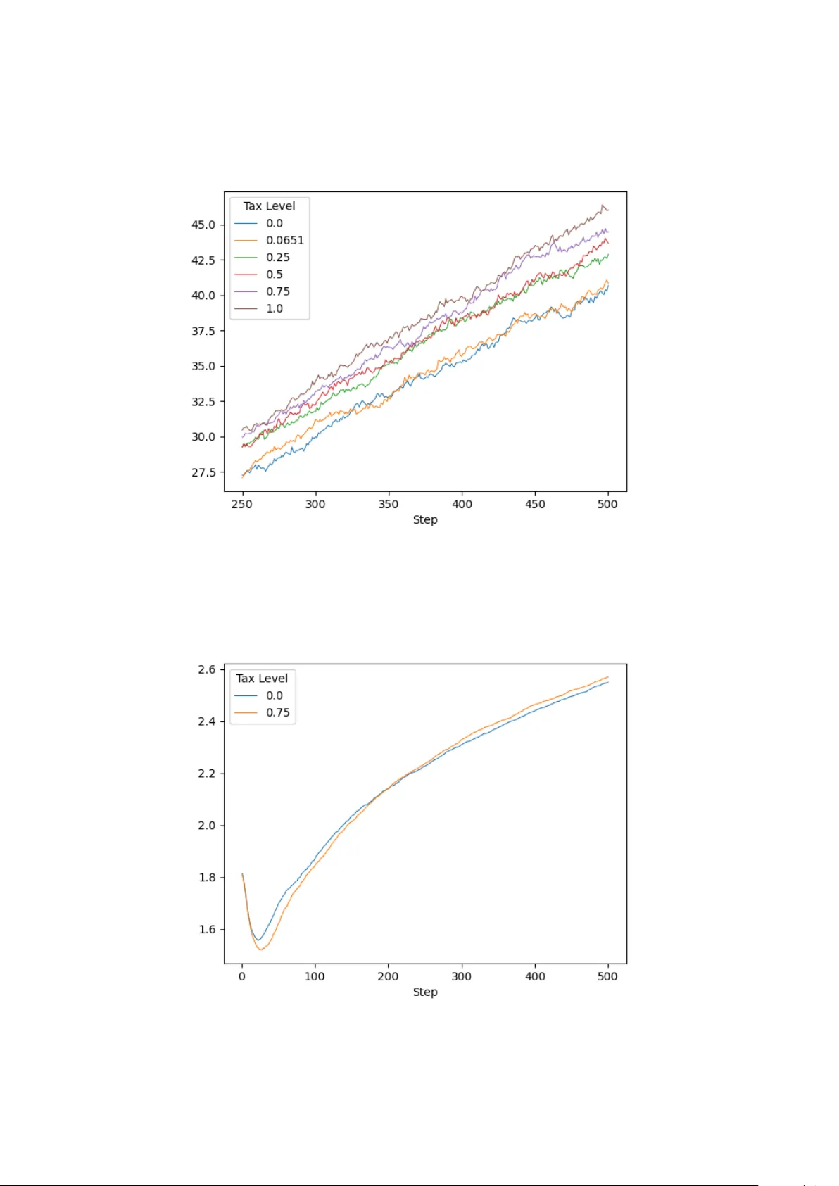
En vironmental polic y in the conte xt of comple x systems: Statistical optimization and sensiti vity analysis for ABMs Dylan Munson a,* , Arijit Dey b , and Simon Mak b a Sanford School of Public Policy , Duke Uni v ersity * Corresponding author: Dylan Munson, dylan.munson@duke.edu, 201 Science Dri v e, Durham, NC 27708 b Department of Statistical Science, Duke Uni v ersity Abstract Coupled human-en vironment systems are increasingly being understood as com- plex adapti ve systems (CAS), in which micro-lev el interactions between compo- nents lead to emer gent beha vior . Agent-based models (ABMs) hold great promise for en vironmental policy design by capturing such complex behavior , enabling a sophisticated understanding of potential interventions. One limitation, ho wev er , is that ABMs can be computationally costly to simulate, which hinders their use for policy optimization. T o address this, we propose a ne w statistical frame work that exploits machine learning techniques to accelerate policy optimization with costly ABMs. W e first de v elop a statistical approach for sensitivity testing of the optimal policy , then le verage a reinforcement learning method for ef ficient policy optimization. W e test this frame w ork on the classic “Sugarscape” model, an ABM for resource harvesting. W e show that our approach can quickly identify optimal and interpretable policies that impro ve upon baseline techniques, with insightful sensiti vity and dynamic analyses that connect back to economic theory . K eywords: agent-based modeling, environmental policy , natural resources, opti- mization, sensiti vity analysis. 1 1 Intr oduction Disorder is at least as old as, and, according to one of the most popular theories, more fundamental than time itself ( Rov elli 2018 ). While the question of to what e xtent this conception of entropy applies directly to social systems rather than only through phys- ical phenomena is still open ( Mavrofides et al. 2011 ), one notable trend in the social sciences has sought to embrace a certain form of disorder in its approach to this type of research, namely , “complexity . ” “Complexity” is a conceptually sticky term with no clear , single definition. One com- mon notion of comple xity places it at the “edge of chaos, ” where deterministic systems with strong sensiti vity to initial conditions gi ve rise to extremely complicated, hard to parse behavior (see, for example, the figure on page 10 of Strogatz ( 2018 )). Mitchell ( 2009 ), ho we ver , distinguishes sev eral common properties of such systems and figures them as “system[s] in which large networks of components with no central control and simple rules of operation giv e rise to complex collectiv e behavior , sophisticated in- formation processing, and adaptation via learning or e v olution” (p. 13). 1 The three properties noted at the end of this definition seem broad enough to be almost redundant but, upon further reflection, ground the study of such systems in a v ery specific tradition of social scientific research, namely computational social science. Computational social science (CSS) can be broadly thought of as a methodological vari- ation on more traditional approaches to sociological and economic problems, applying computational principles instead of closed-form and equation-based ones. These prin- ciples in particular become of use when dealing with comple x data –data which does not admit easy unpacking with closed-form equations because of feedbacks, nonlinearities, causal loops, psychological intricacies, etc.–data which is also usually “large-scale” and often simulated in nature ( Lazer et al. 2020 ). If this definition seems opaque, it is largely because the types of methods subsumed under the heading of “computational social science” are di v erse and wide-ranging. This paper will focus hereafter almost exclusi v ely on one of these methods, agent-based modeling (ABM). In particular , this attention to ABMs is warranted by increasing interest in their ap- plication to problems of public polic y; we here focus on more specific questions of en vir onmental policy , a space within the ABM literature which has under gone greater exploration in recent years but still lacks full methodological clarity . W e here hope to contribute to this bur geoning literature by demonstrating both the practicability of ap- plying ABMs to environment al policy questions, and by applying statistically rigorous techniques to the analysis of model outputs, thus solidifying the procedural underpin- nings of this research space. All that said, it would be a gross misrepresentation of prior research to say that no attempts have been made at applying the science of comple x systems, in any form in- cluding those of agent-based models, to questions of governance and policy . One of the foundational works of computational social science, Epstein and Axtell’ s Gr owing 1 Such a definition applies specifically to complex adaptive systems, which are almost entirely the focus of this work. 2 Artificial Societies , notes the policy implications of the agent-based models of price dy- namics presented in the work. The y cite in particular the power of their non-equilibrium results to challenge con v entional wisdom about the operations of markets ( Epstein and Axtell 1996 ). Indeed, it has been the argument of man y researchers working on the application of comple xity to social systems that it is precisely here where the po wer of such an approach lies: by allowing for adaptiv e and dynamic interactions between micro-le vel actors within the model framework, richer results and more precise pol- icy statements may be made. Existing work on the global sensiti vity and uncertainty analysis of ABMs includes Fonobero v a et al. ( 2013 ); work on statistical inference of parameters has also been done ( G. V . Bobashev and R. J. Morris 2010 ). W e provide a more comprehensi ve literature re vie w of ABMs for polic ymaking in the next section. One key bottleneck with ABMs of complex systems, howe ver , is that their simulation can be computationally costly . Such a cost arises from the need to carefully model for complex and fine-scale interactions in the system. Even for the classic “Sugarscape” model ( Epstein and Axtell 1996 ) in v estigated later in section 5 , an ensemble of hun- dreds to thousands of simulations can take multiple hours to perform. The use of such costly ABMs for policy optimization can thus be computationally v ery intensive, es- pecially when many polic y le vers are considered. This cost can hinder the promise of ABMs for policy optimization in practical applications. T o address this, we pro- pose a ne w statistical framework that lev erages machine learning techniques to accel- erate policy optimization with costly ABMs. In particular , our framework makes use of flexible learning models and reinforcement learning techniques that work well in this “black-box” setting ( Frazier 2018 ), where data are obtained from costly simulator models. W e will first dev elop a statistical approach for testing the sensitivity of the op- timal polic y with respect to state parameters, then make use of a Bayesian optimization reinforcement learning approach ( Chen et al. 2024 ) for ef ficient policy optimization from the ABM. The effecti v eness of this framework will be demonstrated on the clas- sic “Sugarscape” model in Epstein and Axtell ( 1996 ), where we sho w that optimal and interpretable policies can be identified quickly , with insightful sensiti vity and dynamic analyses that can be related back to economic theory . W e be gin in section 2 with a re vie w of e xisting literature at the intersection of com- plex systems and polic y analysis. Section 3 presents the proposed statistical framework for sensitivity testing and policy optimization with ABMs. Section 4 then extends the Sugarscape model in Epstein and Axtell ( 1996 ), which we use as a proof-of-concept ABM for applying the proposed frame w ork. Section 5 in vestigates the policies opti- mized using our method compared to baselines, along with corresponding sensitivity and dynamic analyses. Section 6 concludes. 2 Backgr ound and Literature Re view It has long been understood that human-environment systems and interactions are “com- plex” in the colloquial sense of that word. The extent to which this understanding has spilled over into a more precise, scientific one of complexity is less clear . It is to in- terdisciplinary work, rather than work from a purely social or naturalistic view of the 3 world, that we must turn to truly see this bridge materialize. As just one introductory e xample, in his sweeping work The Gr eat T r ansition: Cli- mate, Disease and Society in the Late-Medieval W orld , economic historian Bruce M.S. Campbell assesses the way in which a variety of social, economic, political, and en vi- ronmental factors aligned to launch a fateful turn in the fortunes of Eurasia around the 14th century . Not least amongst these were the repeated epidemics of the Black Death, long known to have been piv otal in shaping the course of European history . Campbell, ho we ver , goes be yond a myopic analysis of these events, including as well solar c y- cle data from sunspot observ ations and temperature anomalies extracted from bubbles trapped in ice, to name just two. The multiple data sources appealed to in the work, while indicativ e of the need for interdisciplinary understanding, is not the point to em- phasize here, howe v er; it is the way in which Campbell highlights the comple xity of the interactions between different factors, such as disease and climatic anomalies, as be- ing paramount in determining the course of his “Great T ransition. ” No single e vent or ef fect was responsible for the change in Europe’ s fortunes, but it was instead the inter - actions between them that led to system-le v el changes, which in turn shaped the course of ci vilization on the continent. As the author puts it, “[a]t any giv en juncture sev eral dif ferent outcomes were possible depending upon the precise configuration of human and en vironmental forces” ( Campbell 2016 , p. 3). This notion is startlingly close to that of sensitive dependence on initial conditions which is so vital to an understanding of scientific chaos and, by extension, comple xity . Can interactions between people and their en vironment, such as those that brought about the medie v al Great T ransition, be more generally considered complex, then? W e ar gue, as others such as Levin et al. ( 2013 ), Reyers et al. ( 2018 ), and Preiser et al. ( 2018 ) hav e before, that the answer is yes. In the first of these works, the authors posit that social-ecological systems emerge from collectiv e beha vior which percolates to higher le vels of the systems. This thinking fits squarely in the tradition upon which ABMs and complex adaptiv e systems (CAS, complex systems in which system-lev el changes significantly occur through learning or ev olution ( Mitchell 2009 )) are b uilt: micro-le v el interactions coalesce into processes which exhibit behavior that could not easily be pre- dicted from an analysis of the indi vidual agents themselves. From a policy standpoint, ef fecti ve management of such a system requires balancing redundancy , heterogeneity , and modularity to ensure the system is resilient to shocks and losses. The authors further emphasize that nonlinearities present in such systems may gi v e rise to tipping points not well predicted by non-CAS models, as in the case of reef sys- tems, an argument also taken up by Reyers et al. ( 2018 ). Tipping points and re gime changes are well within the purview of complexity and chaos embedded, as they are, in the study of bifurcations (see, for e xample, chapter 3 in Strogatz ( 2018 )). The y are also a topic of major concern in climate change modeling, with small perturbations to v arious en vironmental systems due to human activity potentially leading to qualitativ e changes in the beha viors of those systems ( Lenton et al. 2008 ). Although climate mod- eling is not the focus of the present study , the fact remains that understanding coupled human-en vironment systems requires an acceptance of the fact that underlying dynam- ics are likely nonlinear and complex, and thus difficult to model, especially with more 4 traditional approaches. The benefit of a computational approach (note that numerically solved non-linear mod- els hav e long been a norm in global climate modeling ( McGuf fie and Henderson-Sellers 2001 )) is that complex (or in the case when closed form systems are av ailable, non- linear) processes may be modeled, as long as computational power is suf ficient. In- deed, as computing capacity has increased v astly in recent decades, more disciplines hav e begun to recognize the potential of complexity in solving pressing methodologi- cal questions. The spheres of public policy , including en vironmental policy , hav e been among these. During a 2001 symposium on the topic of the use of ABMs for the simulation of public policy , Lempert ( 2002 ) argued for the use of such models, coupled with “new analytic approaches for decision-making under conditions of deep uncertainty , ” to simulate phe- nomena which cannot be represented with simple mathematical structures. In fact, it is exactly these types of adv ances in the methodology and systematization of the use of ABMs that will allow their use to tackle rich problems of en vironmental concern; it is also the type of contribution which this paper hopes to make. More recent proposals hav e called for the use of ABMs to shape food policy ( Giabbanelli and Crutzen 2017 ) and transportation gov ernance ( Maggi and V allino 2016 ). Still, empirical applications hav e been lagging. One area in which some progress has been made on this front is in the sphere of en- vironmental, and more particularly agricultural, polic y . A commonly used model in this literature is the Agricultural Polic y Simulator (AgriPoliS) ( Happe et al. 2004 ). The model, designed with a German context in mind, is meant to o vercome the limitations of ov erly-aggre gated macroeconomic models which make the analysis of policies im- pacting the micro-le vel dif ficult. The model, ho we ver , does not necessarily have polic y optimization itself in mind; instead, farmers (who are the agents in the model) by as- sumption kno w about major policy changes befor e the y take ef fect. This makes fle xible analysis of exogenous large-scale policy shifts (e.g. regime changes) through sensitivity analysis relati vely straightforward (see, for example, Happe et al. ( 2006 )), but the as- sumptions built in to the model would presumably not allo w internal changes in policy to be optimized. Similarly , the Regional Multi-Agent Simulated (RegMAS) simulates local r esponses to polic y changes, making it a valuable tool for scenario analysis but not necessarily for policy choices ( Lobianco and Esposti 2010 ). Policies are in fact read into this model from external sources rather than being lev ers operated within the model ma- chinery itself, as in the model we present belo w . On the other hand, sensiti vity analysis to various innov ations and changes in model parameters can allow some form of rudi- mentary policy tuning; steps in this direction seem to be made by the designers of the Mathematical Programming-based Multi Agent Systems (MP-MAS) ( Schreinemachers and Berger 2011 ). That model has been used, for example, to measure the effects of better access to credit and improv ed technologies for farmers; the model is in fact able to quantify the ef fects of such policy changes on v arious model outputs such as the pov erty rate ( Schreinemachers et al. 2007 ). As can be seen in this brief surve y , scenario analysis is a common theme with agent-based models, and does allow for polic y tun- ing, but true policy optimization has not been extensi vely tested in the literature to our 5 kno wledge. It is also worth noting that other agent-based models hav e specifically taken up the issue of adaptation to climate change, including amongst agriculturalists. While a thorough re vie w of this literature will thus be left for that work, it has been ar gued that MAS systems of the type pre viously mentioned, as well as ABMs, are well-suited for making policy decisions because of their ability to capture uncertainty and adaptation within the framew ork of the model itself ( Berger and Troost 2014 ). Such simulators ha ve been used to explore, for example, shifts in adapti ve capacity due to climate change in Ethiopia ( Hailegior gis et al. 2018 ). Despite such adv ances, further methodological advances are needed to fully realize the promise of ABMs for polic y crafting. On the one hand, it is worth noting from the outset that polic y should not be designed e xclusi vely based on the recommendation of a single ABM or simulation ensemble (indeed, policy advice should almost ne ver be tied to a single source in any case). ABMs and a comple x systems approach ha ve the ability to challenge con ventional notions of economic and en vironmental dynamics, but should be coupled with other approaches to craft intelligent, fair , and well-founded policy . On the other hand, such methods provide a unique opportunity to simulate a continuum of policy options and optimize over these possibilities. Figure 1 displays one possible way of understanding the relationship between theoretical and empirical foundations and the use of ABMs for the design and implementation of policies. W ith the micro-founded fundamentals of such models in hand, simulation results can provide rich analysis of the impacts of shifting a gi ven policy lev er (or set of le vers) on macro, distributional, and agent-le vel outcomes. Specifically , the methods that we de velop in this paper can be used to (1) test for sensiti vity of model outputs to various potential policy-moderating state v ariables, and then (2) if policy outcomes are determined to be sensiti ve to such v ariables, more thoroughly optimize ov er policy options using carefully-implemented machine learning techniques. T o achie v e this policy optimization goal with ABMs, one k ey challenge is the computa- tional cost of ABM simulations: each run can require minutes or e ven hours to perform for sophisticated models. This can hinder the optimization of such models for policy crafting, as it limits the number of policy choices that one can test from the ABM. T o address this, we propose in the following a ne w frame w ork for policy optimization, which incorporates machine learning techniques to accelerate this optimization proce- dure. Our w ork contrib utes to the kind of policy analysis workflo w described abov e, by le veraging statistical sensitivity testing and reinforcement learning techniques that work well with limited simulation runs from the ABM. Our methodology is highly adaptable to a multitude of use cases beyond the highly stylized en vironmental and natural re- source model we use in this work. W e thus contribute not only to the literature on agent-based modeling and statistical optimization of such models, b ut also the field of policy analysis more generally , where such models can be of great use (as is evidenced by the literature abov e). 6 3 Methods: A Statistical Framework f or Sensitivity T est- ing and Optimization of ABMs W e here present the proposed ML-based statistical frame work for sensiti vity testing and subsequent policy optimization using complex ABMs. W e first outline in subsec- tion 3.1 our sensitivity testing approach, which lev erages statistical hypothesis testing techniques with a flexible ML model called a Gaussian process Gramac y 2020 . W e then describe in subsection 3.2 a reinforcement learning approach that uses this ML model to guide policy optimization from the costly ABM. W e first establish some notation. Suppose the ABM takes in two types of input vari- ables: (i) policy (or “choice”) v ariables x ∈ R d , which parametrize a discrete or con- tinuous policy space P , and (ii) state v ariables θ ∈ R p , which parametrize what we will sometimes refer to as system “state v ariables, ” roughly in line with the corresponding concept from optimal control theory ( Leonard and V an Long 1992 ). For example, to in v estigate agricultural resilience, an ABM may take in inputs x that dictate dif ferent adaptation subsidy policies, as well as inputs θ that model for varying household and en vironmental characteristics. Gi ven v ariables x and θ , we model the simulated response from the ABM as a realiza- tion from the random v ariable G ( x, θ ) , as such a response is inherently stochastic due to randomness in initial model states, bounded rationality in behavioral patterns, and other randomness inherent in agent decisions and the model en vironment. For example, G ( x.θ ) may model the distrib ution of wealth or welf are in a population, from which the ABM output is simulated. A reasonable formulation of the policy optimization problem might then be: x ∗ ( θ ) := arg min x f ( x, θ ) , f ( x, θ ) := Ψ { G ( x, θ ) } , (1) where f is the target objectiv e function to minimize. Here, Ψ is a functional that maps the random variable G onto a real number . Common choices of Ψ include the distribu- tion mean Ψ( G ) = E ( G ) (e.g., the average wealth in the population), or the distrib ution 5%-quantile Ψ( G ) = Q 5% ( G ) (e.g., the wealth lev el belo w which 5% of the population falls). In our later experiments, we employ the distrib ution mean for Ψ as a proof- of-concept. Our proposed approach can be used analogously for either minimizing or maximizing f ; for bre vity , we presume minimization in what follo ws. A ke y challenge for the policy optimization problem ( 1 ) is that, for a complex ABM, each e v aluation of the objecti ve function f ( x, θ ) can be computationally costly . Gi v en a choice of ( x, θ ) , the e v aluation of f ( x, θ ) requires many simulations from the ABM, i.e., sample draws from the distribution G ( x, θ ) , to reliably compute the functional Ψ { G ( x, θ ) } ; we pro vide guidance on the number of sample draws later in section 3.3 . For sophisticated ABMs, the cost of performing each simulation run can be non- negligible, particularly with many agents in the model, fine-grained agent representa- tions ( Schwarz and Ernst 2009 ), or increased fidelity in modeling physical en viron- ments (e.g., water flo w dynamics; Dawson et al. , 2011 ). This means a single ev aluation of f ( x, θ ) can require minutes or e ven hours, which greatly limits the number of ( x, θ ) 7 combinations (i.e., dif ferent combinations of policies and state parameters) that one can test from the ABM. This makes the target problem of sensitivity testing for f and its subsequent policy optimization highly dif ficult problems. In the ML literature, the property that f is unkno wn and costly to e v aluate is referred to as a “black-box” function ( Frazier 2018 ). The analysis and optimization of such black- box functions is challenging, and require carefully-designed ML techniques that work well with limited ev aluations of f . T o this end, we present two ML-based approaches for ef fecti ve sensiti vity testing and polic y optimization from costly ABMs. 3.1 Sensitivity T esting First, we consider a problem inherent to the black-box nature of the function f : is the optimal choice of x , x ⋆ , dependent on, or sensitive to a particular value (or values of) the state parameter(s) θ ? In other words, if θ may take on certain values, or perhaps in a formulation that is more rele v ant to the questions at hand, if the actual value of θ is uncertain but known to be within some range, is x ⋆ ( θ ) ≈ C for all choices of θ , where C is some constant? Or is x ⋆ truly a function of θ ? If the answer to this last question is “yes, ” then optimal policy choices could vary drastically ov er ev en minor changes to the model state and initial conditions. For this reason, we would need to be e xceptionally careful in optimizing over ensembles of model runs which may ha ve different initial conditions, and ov er dif ferent possible v alues of θ . The above notion of sensiti vity is directly related to the idea of additi vity for f . The function f ( x, θ ) is additive if it can be written as f ( x, θ ) = g 1 ( x ) + g 2 ( θ ) for some functions g 1 and g 2 . Note that the additivity of f immediately implies that the optimizer of f , namely x ⋆ , is not dependent on θ . Ho we ver , if the function is instead non-additive , i.e., f ( x, θ ) = g 1 ( x ) + g 2 ( θ ) + g 3 ( x, θ ) for some appropriate functions g 1 , g 2 , g 3 , where g 3 ( x, θ ) is non-zero, then the optimizer x ⋆ ( θ ) may indeed be dependent on θ . W e present next a statistical procedure for testing additi vity on the black-box function f , which allo ws us to in vestigate the sensiti vity of the optimal solution x ⋆ to the state v ariables θ . Suppose we simulate data of the form D = { f ( x 1 , θ 1 ) , · · · , f ( x n , θ n ) } from the ABM, where ( x 1 , θ 1 ) , · · · , ( x n , θ n ) are tested combinations of policy and state variables. Here, the number of tested combinations n is again limited due to the costly nature of func- tion e v aluations. Our statistical hypothesis test makes use of Gaussian process ( Gra- macy 2020 ) models, which are flexible Bayesian ML models broadly used in scientific applications, e.g., aerospace engineering ( Miller et al. 2024 ) and space science ( Li and Mak 2025 ). A k ey appeal of GPs is that the y provide effecti v e, reliable and uncertainty- aw are learning with a limited sample size n , all of which are needed for our sensiti vity testing and policy optimization goals here. Formally , a GP model on f can be denoted as: f ∼ GP { µ, K ( · , · ) } , (2) where µ is a scalar mean hyperparameter , and K ( · , · ) is a scalar-v alued kernel function. 8 A popular kernel choice is the squared-e xponential kernel ( Gramac y 2020 ): K (( x, θ ) , ( x ′ , θ ′ )) = σ 2 exp    − d X l =1 x [ l ] − x ′ [ l ] ψ x,l ! 2 − p X l =1 θ [ l ] − θ ′ [ l ] ψ θ,l ! 2    , (3) where x = ( x [1] , · · · , x [ d ] ) and θ = ( θ [1] , · · · , θ [ p ] ) are the vectors of policy and state v ariables, respecti vely . Here, σ 2 is a k ernel v ariance hyperparameter , and { ψ x,l } d l =1 and { ψ θ,l } p l =1 are kernel length-scales that model the importance of different policy and state v ariables on f , respectiv ely . The model hyperparameters µ , σ 2 , { ψ x,l } d l =1 and { ψ θ,l } p l =1 can be learned from the simulated data D . The class of functions modeled by a GP of this form can be shown to be nonparametric and highly flexible ( V an Der V aart and V an Zanten 2011 ). W ith this, suppose the true function f ( x, θ ) is additi v e in nature. Then a reasonable learning model for f may be f ( x, θ ) = g 1 ( x ) + g 2 ( θ ) , where g 1 ∼ GP { µ 1 , K 1 ( · , · ) } and g 2 ∼ GP { µ 2 , K 2 ( · , · ) } . Here, K 1 ( x, x ′ ) is a kernel depending on only policy v ariables x , and K 2 ( θ , θ ′ ) is a kernel depending on only state v ariables θ . For kernel K 1 (or kernel K 2 ), the squared-e xponential form ( 3 ) can be used with only the length-scale hyperparameters { ψ x,l } d l =1 (or only the length-scale hyperparameters { ψ θ,l } p l =1 ). W e shall call this the null model. Con versely , suppose the true f is non-additiv e. Then an alternate model might be f ( x, θ ) = g 1 ( x ) + g 2 ( θ ) + g 3 ( x, θ ) , where g 1 and g 2 follo w the abov e GP models, and g 3 ∼ GP { 0 , K 3 ( · , · ) } , where the kernel K 3 (( x, θ ) , ( x ′ , θ ′ )) is ov er both x and θ . F or kernel K 3 , we adopt the squared-exponential form gi v en in ( 3 ), where its length-scale hyperparameters are distinct from those for K 1 and K 2 . W e shall call this the alternative model. All kernels K 1 , K 2 and K 3 share the same kernel v ariance σ 2 . Hyperparameters for both the null and alternati v e models can be learned from data by maximizing their likelihood functions ( Casella and Ber ger 2024 ). Our hypothesis test for additi vity can then be formalized as follows. Define the “null hypothesis” as the hypothesis where f follo ws the abov e additiv e null model. Define the “alternati v e hypothesis” as the hypothesis where f follows the broader non-additiv e alternati ve model. W e adopt a likelihood ratio test (LR T ; Casella and Berger , 2024 ) to test whether there is sufficient e vidence from data D to reject the null hypothesis of an additi ve f . The LR T uses the test statistic: Λ = − 2( l 0 − l 1 ) , (4) where l 1 is the log-likelihood of the alternati ve model fitted using data D , with model hyperparameters learned via maximum likelihood, and l 0 is the log-likelihood of the null model fitted using data D , with hyperparameters learned in a similar fashion. The full likelihood e xpressions under a GP can be found in Gramacy ( 2020 ); they are omit- ted here for brevity . Note that a larger test statistic Λ gi ves stronger e vidence that addi- ti vity is violated for f , as this implies the log-likelihood under the alternati ve model is considerably larger than that under the null model. One can prove ( Casella and Berger 2024 ) that, under the null model, the test statistic Λ follows approximately a chi-squared distribution χ 2 ν with ν = d + p degrees-of- freedom, since the non-additi ve alternativ e model has d + p additional hyperparameters 9 ov er the additiv e null model. The p-v alue for this test can then be computed as the probability P ( χ 2 ν > Λ) . A small p-v alue suggests that, under the null hypothesis of an additi ve f , the probability of observing the data D is low . This thus provides statistical e vidence against the additi vity of f , and suggests that the optimal solution x ⋆ may indeed be sensitiv e to the state variables θ . Con v ersely , a large p-v alue giv es little statistical e vidence against the additi ve nature of f , which in turn suggests the optimal solution x ∗ may be insensiti ve to θ . 3.2 Bayesian Optimization Suppose we find, from the abov e sensitivity test, that the optimal policy decision x ⋆ ( θ ) is indeed sensiti v e to the state parameters θ . T o further in vestigate this, we may wish to find, for different choices of θ , ho w its corresponding optimal solution x ∗ ( θ ) from ( 1 ) changes. Again, finding x ∗ ( θ ) is a highly challenging problem, since f is a black-box function with no closed-form expression and is costly to e v aluate, requiring simulations from the ABM. T o solve ( 1 ), we need to lev erage black-box optimization algorithms that work well with limited e v aluations on f . Bayesian optimization (BO; Frazier , 2018 ) provides an ef fecti ve solution. BO is a re- inforcement learning approach for optimizing black-box functions, with successful ap- plications in machine learning ( Snoek et al. 2012 ) and engineering design ( Kim et al. 2025 ). For a fixed choice of θ , the idea is to use existing e v aluations on f to construct a so-called “acquisition function” a ( x ) , which le verages a fitted learning model to quan- tify the attracti veness of a potential ev aluation point ( x, θ ) for optimization. Next, the function f is ev aluated at the point that maximizes this acquisition function a ( x ) . The learning model is then refit with the new data from the ABM, and the above sequential sampling procedure is repeated until a satisfactory optimization solution is obtained. W e will employ a popular BO approach called Expected Improvement (EI; Jones et al. , 1998 ) for optimizing x ∗ ( θ ) , which lev erages the GP model introduced earlier on the objecti ve function f ( · , θ ) . Let θ be the fixed set of considered state v ariables. Suppose f has already been e v aluated at the input combinations 2 ( x ′ 1 , θ ) , · · · , ( x ′ m , θ ) from the ABM. The EI acquisition function is then defined as: EI ( x ) = Φ f min − ˆ f ( x ) s ( x ) ! ( f min − ˆ f ( x )) + ϕ f min − ˆ f ( x ) s ( x ) ! s ( x ) . (5) where Φ and ϕ are the cumulativ e and probability density functions of a standard normal distribution, respectiv ely , and f min = min i =1 , ··· ,m f ( x ′ i , θ ) is the smallest observed v alue of the objecti v e function. Here, ˆ f ( x ) and s ( x ) are the predicted v alue of f ( x, θ ) from the fitted GP model and its corresponding predicti ve standard deviation; see Gramacy ( 2020 ) for their full expressions. EI ( x ) can further be viewed as the expected objecti ve improv ement from a ne w function e v aluation at inputs ( x, θ ) ; see Chen et al. ( 2024 ). W ith this, the next ev aluation point ( x ′ m +1 , θ ) is selected to maximize the expected improv ement acquisition, i.e., x ′ m +1 = arg max x EI ( x ) . Points selected by maximizing 2 Here, the notation x ′ i is used to distinguish these ev aluation points from those used in section 3.1 . 10 EI ( x ) capture the “exploration-e xploitation trade-of f ” ( Liu and Mak 2025 ) fundamental in reinforcement learning: the maximization of the first term in ( 5 ) tar gets x with small predicted objecti ves ˆ f ( x ) (i.e., exploitation), whereas the maximization of the second term targets x with large predictiv e uncertainties s ( x ) (i.e., exploration). The ABM is then simulated at the optimized point ( x ′ m +1 , θ ) , the GP model is re-fit, and the abo ve sequential sampling procedure is repeated until a good solution is found for optimizing ( 1 ). For optimizing black-box ABMs, this BO procedure can be considerably more ef ficient computationally than random sampling of the policy v ariables, as we sho w later in section 5.2 . 3.3 Algorithm Statements Algorithms 1 and 2 outline the detailed steps for our proposed sensitivity testing and policy optimization approaches. W e pro vide a brief discussion of each in the follo wing. Our sensitivity testing algorithm (Algorithm 1 ) begins with selecting the initial ev alua- tion points { ( x i , θ i ) } n i =1 for the black-box function f . Follo wing the rule-of-thumb for GP modeling ( Loeppky et al. 2009 ), we recommend the number of ev aluation points be set as n = 10( d + p ) , where d + p is the number of policy and state variables in the ABM. These points should further be selected from a Latin hypercube design (LHD; Stein , 1987 ), which offers improved performance compared to random sampling. The ABM is then run at each of these points, and the objective f is ev aluated via Equation ( 1 ). Note that, for a giv en ( x, θ ) , e v aluating f ( x, θ ) requires many ABM simulation runs, i.e., sample draws from the distrib ution G ( x, θ ) . In our experiments later , we find that 150 sample draws provide suf ficient precision for good sensitivity testing and policy optimization performance. Next, using the simulated data from the ABM, namely D = { f ( x i , θ i ) } n i =1 , we fit the GP models under the null (additi ve) and alternativ e (non-additiv e) hypotheses. Hyper- parameters for these models are trained via maximum likelihood ( Casella and Berger 2024 ), where likelihood optimization is performed via the Adam optimizer ( Kingma and Ba 2014 ). Model training of all GPs is performed via the GPyTorch package ( Gardner et al. 2018 ) in Python. The LR T statistic Λ is then computed from ( 4 ), and the test p-v alue is e v aluated as the probability P ( χ 2 ν > Λ) . Finally , this probability is compared with a pre-set significance lev el α (typically taken to be 0.05) to determine whether there is enough statistical e vidence to reject additi vity in f . Our Bayesian optimization algorithm (Algorithm 2 ) then aims to identify the optimal policy decision x ∗ ( θ ) for a fixed choice of state variables θ . For initial model learning, we first ev aluate f at the points { ( x ′ i , θ ) } m i =1 , where the points x ′ 1 , · · · , x ′ m are selected from an LHD. Here, a small number of initial ev aluations m is sufficient (e.g., m = 5 ), as the Bayesian optimization procedure adds in sequential ev aluations after . W ith this initial data, we fit a GP model on the objectiv e function f ( · , θ ) , and optimize its hyperparameters via maximum likelihood ( Casella and Berger 2024 ). Ne xt, we select the next e valuation point x ′ m +1 by maximizing the acquisition function EI ( x ) in ( 5 ) using the Adam optimizer ( Kingma and Ba 2014 ), and e v aluate f at the new point ( x ′ m +1 , θ ) via the ABM. The GP model is then re-fit with this ne w data, and the above 11 Algorithm 1: Sensiti vity T esting of Optimal Policy Require: Number of ev aluation points n , significance le v el α 1: Select e v aluation points { ( x i , θ i ) } n i =1 from an LHD. 2: Run the ABM at these e v aluation points to obtain data D = { f ( x i , θ i ) } n i =1 . 3: Null Model : Using data D , optimize hyperparameters for the additi v e GP via maximum likelihood using the Adam optimizer ( Kingma and Ba 2014 ). Define l 0 as the log-likelihood of this model with optimized hyperparameters. 4: Alternative Model : Using data D , optimize hyperparameters for the non-additi v e GP via maximum likelihood using the Adam optimizer ( Kingma and Ba 2014 ). Define l 1 as the log-likelihood of this model with optimized hyperparameters. 5: Compute the LR T statistic Λ = − 2( l 0 − l 1 ) , and compute the p-v alue ς = P ( χ 2 ν > Λ) , where chi 2 ν is the chi-squared distribution with ν = d + p degrees-of-freedom. 6: If ς < α , there is statistical e vidence that the optimal polic y x ∗ ( θ ) is sensitiv e to state v ariables θ . Otherwise, there is insuf ficient statistical e vidence for sensiti vity . Algorithm 2: Policy Optimization via Bayesian Optimization Require: Fixed state v ariables θ , number of initial e v aluation points m , number of sequential BO iterations M 1: Select initial e v aluation points { ( x ′ i , θ ) } m i =1 from an LHD. 2: Run the ABM at these initial points to obtain data D ′ = { f ( x ′ i , θ ) } m i =1 . 3: f or t = 1 , · · · , M do 4: Fit a GP model on the data D ′ , with model hyperparameters optimized via maximum likelihood. 5: Optimize the next polic y v ariables to be e v aluated as x ′ m + t = arg max x EI ( x ) using the Adam optimizer ( Kingma and Ba 2014 ). 6: Run the ABM at the ne w input point ( x ′ m + t , θ ) and e v aluate f ( x ′ m + t , θ ) . 7: Update the training data D ′ ← D ′ ∪ { f ( x ′ m + t , θ ) } . 8: end for 9: Retur n: The best observed polic y x ∗ = arg min x ∈{ x ′ 1 , ··· ,x ′ m + M } f ( x, θ ) . sequential sampling procedure is repeated until a good optimization solution is found. For our later e xperiments, we find that M = 100 iterations of this sequential procedure is sufficient for optimization, although this should be determined on a case-by-case basis gi ven computational time constraints. In our implementation, Algorithm 2 is performed using the Python package BoTorch ( Balandat et al. 2020 ). 12 4 Pr oof-of-Concept Model: P ollution on the Sugarscape 4.1 Model Description W e now apply the proposed framew ork for sensiti vity testing and polic y optimization to a proof-of-concept application. In what follows, we will adopt and extend the Sug- arscape model, described in Chapter 4 of Epstein and Axtell ( 1996 ). The classic soft- ware for building such an agent-based model is NetLogo, b ut we have here used an extended version of the model constructed using the Python-based mesa frame w ork ( Kazil et al. 2020 ) to improv e reproducibility . A version of the base mesa model, to which we made adjustments in order to incorporate pollution and mitig ating policy op- tions, is av ailable at https://mesa.readthedocs.io/latest/examples/adv anced/sugarscape_ g1mt.html . In the Sugarscape model, space is composed of a grid cell lattice on which agents mo ve. Each grid cell is endo wed with a resource, called by con v ention “sugar” and “spice, ” which are harvested by the agents and which regro w at a constant rate over time. In our version of the model, the resources gro w back at a rate of 1 unit per time step, up to a pre-specified maximum amount that differs between cells. Agents will trade sugar for spice under certain conditions, and also mov e to ne w cells based on welfare-maximizing principles. 3 Agents harv est all the resources on a grid cell which the y occup y at a gi v en time step of the model. They also must consume sugar and spice, and if one of these resources is exhausted for the agent, they die. Thus the rule for agent movement, as gi ven in Epstein and Axtell ( 1996 ), pp. 98-99, is: 1. Look as far as vision permits in each cardinal direction. 2. T aking as feasible only unoccupied positions in the lattice, find the nearest posi- tion that maximizes welfare. 3. Move to that position. 4. Harvest all sugar and spice at that location. The trade rule is more complicated and will not be fully described here, but see the footnote abo ve for a concise explanation, and Epstein and Axtell ( 1996 ), p. 105 for a detailed one: essentially , when the MRS crossing condition is met, the price is calcu- lated as the geometric mean of the two agents’ MRS’ s, and quantities to be exchanged are determined by those prices. Trade then occurs as long as the MRS crossing condi- tion is not violated and welfare increases for both agents. Figure 2 displays the initial distribution of sugar and spice in the model. As in the original formulation by Epstein and Axtell, there are two sugar “hills” and two spice “hills, ” one in each quadrant of the grid. W e no w add an additional principle to the model: sugar is a dirty good, in the sense that both the harvesting and the consumption of sugar produces pollution on the grid cell 3 In particular: 1) agents trade when they encounter one another on the lattice, and their marginal rates of substitution (MRS) between sugar and spice are not equal; 2) agents “search” neighboring cells (within a specified horizon) and mov e to the one that will maximize their welfare. 13 where this occurs. In this sense, sugar has both a production and consumption external- ity associated with it. Spice does not produce any pollution. Again, as in Epstein and Axtell’ s initial formulation, the pollution rule is simple: pollution occurs at rate β . If ρ is the metabolic rate of sugar for a gi ven agent, and s is the amount of sugar harvested on a grid cell, 4 then total pollution at time step t , p t , is gi ven by: p t = p t − 1 + β ( s + ρ ) . (6) Figure 3 sho ws the final pollution distribution ov er the model lattice for one 500-step simulation. The plot also provides a reference for the (unitless) pollution distribution, which is important when setting the bounds for possible v alues of our sug ar production cap (see belo w). Pollution has two direct ef fects with which we are concerned. One, pollution adversely impacts the welfare of agents, i.e. ∂ U /∂ p < 0 . 5 Second, through its effect on utility calculations, pollution impacts agents’ decisions about where to move, as cells with more pollution are less desirable. In particular , as in the utility function in general, it is the ratio of sugar (and spice) to pollution which agents care about. It is worth noting that, despite the fact that the utility function for agents can be written do wn, in general a closed form of the model does not exist. This is in part due to the randomness inherent in the initial configuration of the model, which makes it difficult to predict a priori ho w emergent properties of the system, like the welfare distribution, will ev olv e over time. At the same time, agents hav e imperfect information because they cannot “see” the state of the entire lattice at an y giv en point of time, and are in fact heterogeneous over how imperfect this information is (specifically , ho w far out their vision permits them to see) and ov er other characteristics, such as their metabolic re- quirements for surviv al. In this sense, we can refer to the Sug arscape model as a “black box, ” and shall do so throughout this paper: although a set of rules can be written down that may help interpret why certain results and features of the model emerge, neither total prediction nor total understanding of causal mechanisms is generally possible with this complex v ersion of the model. 4.2 P olicy Options As one may expect from both real experience and prior economic theory , the introduc- tion of pollution qualitativ ely changes model outputs and processes, in general to the detriment of the agents in the model. Figure 4 , for example, shows that as the pollu- tion rate increases, fewer agents tend to surviv e to the end of the model run. Figure 5 demonstrates that, furthermore, the Gini coefficient, a measure of inequality that is 4 Only one unit of sugar is consumed at each time step of the model, so this quantity drops out of the equation. 5 This does not appear to be the case in Epstein and Axtell’ s original model. In their formulation, pollution seems only to enter the utility function insofar as the utility function is the metric based on which decisions about where to mov e are made; that said, Epstein and Axtell’ s model did not, at baseline, return the utility of each agent as a principal measure. They were more concerned with price dynamics. 14 increasing in the ske wness of the welfare distribution in the agent population (see, e.g., Lerman and Y itzhaki , 1984 ), can be quite high at increased pollution rates. W e thus introduce sev eral policy parameters into the model which aim, to one degree and in one way or another , to mitigate the le vels of pollution in the lattice and/or pollu- tion’ s impact on the agents. The four policy le vers are: 1. Production cap on sugar : A simple cap on the level of sugar that can be har- vested by an agent in a single period. The cap is based on the lev el of pollution in a giv en cell: if the pollution lev el is abov e the giv en threshold, no sugar may be harvested on the cell in that period. 2. Reinv estment subsidy to spice : Some amount of the capped sugar growth is assumed to be rein vested as a small subsidy of spice to the agent; that is, when this parameter is nonzero, capped sugar growth is viewed as gro wth that can be di verted back to the “consumer” (i.e., an agent). This occurs at a constant lev el– if no sugar can be harvested because pollution is too high in a cell, a specified amount of spice is gi ven back to the consumer . 6 3. T ax on the trade of sugar : A simple tax on the price of sugar for each sugar- spice trade that occurs. 4. T ax on sugar consumption : An agent must pay extra to consume sugar (based on their metabolic rate), ho we ver this amount is returned to them as extra spice; this is thus another form of “limit-and-rein vest. ” The polic y options were chosen to reflect both a v ariety of real-life en vironmental poli- cies as well as dif fering le vels of interv ention with differing degrees of ef fects on agent welfare and survi val. For example, policy option (1) should ha ve quite a large impact relati ve to the others with regards to agent surviv al, because it directly limits the amount of one of the goods that can be consumed by the agent. On the other hand, it finds a real-life counterpart in, for instance, hard limits on carbon emissions that are fav ored by many experts for keeping anthropogenic global warming below a certain lev el. A tax on sugar trade would be similar in this sense to a tax on the actual exchange of carbon-intensi ve goods, while the tax on sugar consumption would be analogous to a tax that targets consumers of such goods but returns this tax to them as a subsidy for clean alternativ es (e.g., imagine a tax on disposable products that funds a subsidy for reusable alternati ves). 5 Results W e now apply the proposed statistical framew ork for sensitivity analysis and policy optimization to the abov e Sugarscape model, to in vestigate optimal combinations of policy options described in subsection 4.2 . In what follows, we employ the optimiza- tion of sev eral dif ferent objecti ve metrics, including mean welfare in the population 6 Unless otherwise stated, for all models run below , this policy was not optimized but fixed at a lev el of 0.5. W e list it here for completeness but thus consider only the other three main polic y options for the reasons described in the next section. 15 of agents, survi val rate of the agents, and the welfare distribution in the population of agents. W e first consider sensitivity testing results, then in vestigate how such sensiti vity af fects optimal policy decisions and model dynamics. 5.1 Sensitivity T esting W e first test, using the procedure outlined in subsection 3.1 , whether the considered policy options are indeed sensitiv e to each of the three state v ariables: the pollution rate, the minimum initial endowment le vel of an agent (i.e., the lowest possible amount of resources that an agent can randomly start with), and the maximum metabolism rate of an agent (i.e., the highest lev el of consumption required for an agent to survi ve, which is also randomly assigned). The pollution rate was chosen here because, naturally , we may expect that how much pollution is generated by each unit of production and consumption will impact ho w much “policy forcing” is required to achiev e a giv en le vel of the objectiv e. Similarly , if agents have to consume more or start with a lo wer wealth, a giv en objectiv e may be harder to reach with the same policy settings. This sensiti vity is in vestigated for each of the three considered objectiv es: namely , surviv al rate, welfare, and the Gini coefficient. T o briefly summarize our results, we find robustly that all objecti ves are sensiti ve to all three of the state v ariables, with the exception of two cases, both relating to the minimum initial endo wment. T ables 1 - 3 sho w , for each of the three state v ariables, the corresponding sensitivity test statistics Λ and their p-values for each choice of objectiv e, i.e., surviv al rate (SR), welfare (W), and Gini coef ficient (G). This sensitivity test was performed using n = 40 e valuation points, following the rule-of-thumb in section 3.3 . The test p-value is e v aluated from a chi-squared distrib ution with ν = d + p = 4 de grees-of-freedom. The simulation of such data from the ABM required just under 11.5 hours of computation time (parallelization w as not possible here due to the nature of the experiments run, but 40 cores and 120 GB of memory were used nev ertheless). This shows that, even for a relati vely simple ABM, the computational cost of data generation can be quite high. For two of the state variables, pollution rate and maximum metabolism, we see that the test p-values are all nearly zero (and certainly belo w the significance lev el of α = 0 . 05 ), which suggests strong statistical evidence that optimal policy choice is sensiti ve to both pollution rate and maximum metabolism for all objectiv e choices. In other words, both the maximum metabolic rate and the pollution rate of the agents in the population could be considered strong moderators of the optimal policy choice, when considering survi v al rate, welfare, and inequality as objecti ves to optimize. The case for the minimum agent endowment (see T able 2 ) is more nuanced. From this table, we see that when welfare is the objective, the test p-v alue is nearly zero, which suggests that the optimal policy can be highly sensiti ve to the minimum endowment. This makes sense, since a society with a different distribution of minimum wealth lev els but the same distribution of maximum wealth lev els will naturally hav e different av erage welfare lev els (which is our main welfare measure). In other words, if there are more or less ov erall resources in the population at the start of the model run, we should e xpect this to change overall welfare by the end of the model run, which is where we measure 16 sensiti vity . When inequality or survi val rate is the objectiv e, howe ver , we see that the test p-v alues can be large (above the significance lev el of α = 0 . 05 ), which suggests a lack of statistical e vidence for sensitivity . One reason is that, as will be demonstrated in our dynamic analysis in subsection 5.3 , inequality and surviv al rate very quickly settle into an equilibrium during an y gi ven model run. This means that shifts in the bottom of the starting wealth distribution should matter less for the end states of these variables, as seen in the fact that for survi val rate and the Gini coef ficient, the minimum endo wment is not a strong moderator of optimal policy . Unlike the pollution rate and metabolism, the endo wment minimum only determines the starting amount of resources, but does not impact agent beha vior at eac h model step . Thus, the result that model end states are not as strongly moderated by the endo wment v ariable is quite intuiti ve. The abov e analysis sho ws that the optimal policy for the considered model is indeed sensiti ve to v arious state variables (though for minimum endowment, less sensitiv e for certain objectiv es), if our interest lies in the end state of the model. In vestigating how this optimal policy changes ov er the state variable space is thus of interest. This is particularly important when there are uncertainties associated with the considered state v ariables. For example, when empirically calibrating the pollution rate from real-world data, one may ha ve considerable uncertainty on the estimated parameter , and exploring ho w the optimal policy changes for dif ferent plausible choices of this rate is thus impor - tant. An efficient method for such exploration is our proposed Bayesian optimization approach. 5.2 P olicy Optimization In the following, we consider jointly optimizing ov er three of the policy v ariables de- scribed above: the trade tax, the consumption tax, and the production cap on sugar . Using the notation from section 3.2 , these policy v ariables will be referred to as x . The rein vestment amount is fixed at 0.5 to simplify analysis, since it would of course be optimal to con vert as much sugar as possible into spice and return it to the consumer (i.e., the polic y should not be binding). Howe ver , if this con version is thought of as a technology that is unlik ely to change o ver the course of a model run, and if the regro wth rate of resources is constant across cells and time, then it makes sense to lea ve this pol- icy at a constant v alue that is not dependent on the cell’ s total amount of each resource nor the agents’ metabolism. Furthermore, to improve numerical stability , the range of possible values for the taxes was narro wed do wn to the closed interval between 0 and 1. For the sugar production cap, we test values between 6 and 15. 7 Note that a higher cap reflects a less binding polic y , as this allows for more pollution on each grid cell. The pollution rate is fixed at 20% for all model runs. Figures 6 - 8 show the progression of our Bayesian optimization algorithm (Algorithm 2 ), using m = 5 initial ev aluation points and M = 100 subsequent sequential ev aluation points. As an initial pass, three different objecti ves (unconstrained) were in vestigated. The first is a simple welfare maximization procedure, where social welfare is taken as 7 These bounds were chosen heuristically based on results from prior model runs; for instance, it was observed that setting the cap much belo w 6 resulted in all agents dying in most model runs. 17 the average welfare across all agents. The second is maximization o ver the surviv al rate of agents in the model, calculated simply as the number of agents still ali ve at the end of the 500-step model run divided by the initial number of agents (200 in all cases). Finally , we compute and minimize the Gini coef ficient of our simulated society using the welfare distribution in the surviving agent population, i.e., we aim to minimize the inequality in the population. Each figure sho ws the optimization of a different objec- ti ve. In these plots, the black horizontal dashed lines sho w the computed v alue of the objecti ve when no policy is implemented; that is, when both taxes are set to 0 and the production cap is set to infinity . These plots rev eal sev eral interesting observations. First, in all cases, we see that the Bayesian optimization procedure con verges quite quickly to an optimal solution; such a solution is generally found within 60 sequential iterations of the procedure, with little- to-no improv ements made in subsequent iterations. This is typical of BO algorithms, which can find optimal solutions with limited ev aluations of the black-box objectiv e function, as long as there are not many v ariables to optimize ov er ( Chen et al. 2024 ). Second, the optimized policies of fer considerably improv ed objectives over the no- policy baseline, which shows the potential of BO for identifying promising new pol- icy options from the black-box ABM. Interestingly , such an improvement is smallest for the surviv al rate. As is noted in the follo wing subsection, survi v al rate tends to be particularly lo w in the long-run regardless, at the very least, of trade tax lev el, poten- tially due to the weakness of some instruments relativ e to the objectiv e. Finally , it is important to note here the computational cost of ABM simulation for this optimization procedure. T o optimize over welfare, for example, ev aluations of the black-box objec- ti ve f required nearly 3 hours of computation, on a 32-core processor with 64 GB of memory . This shows that, ev en for a relativ ely simple ABM, the computational cost of e v aluating the desired objecti ve can make policy optimization highly challenging; our Bayesian optimization approach provides a solution to this bottleneck. T o gauge the effecti veness of our BO procedure, another baseline method may be to simply select policy points at random over the decision space, run the ABM at such points to ev aluate the objectiv e f , then take the tested policy point with the best sim- ulated objectiv e. Figure 9 shows the comparison of BO with this random benchmark for optimizing the Gini coef ficient, where both methods are compared on M = 50 se- quential iterations to speed up computation. W e see that, at the end of the sequential procedure, the optimal policy found by the random baseline has a considerably higher Gini coef ficient (around 0.205) than that found by the BO procedure (around 0.170). Indeed, throughout the sequential procedure, BO largely dominates the random base- line; there is only a brief period where the random baseline yields better performance due to chance. This improv ement of BO over random points is in line with the literature ( Frazier 2018 ), and highlights the importance of a carefully-trained acquisition function to guide the sequential optimization of a black-box ABM. Next, we inspect the corresponding optimal policies found by the BO algorithm for each choice of objectiv e, which are reported in T able 4 . Again, sev eral interesting observ ations can be gleaned. First, for all objecti ves, the optimized policy has v ery low le vels of trade tax. This suggests, particularly in light of the findings regarding this tax 18 in the next section, that the trade tax is a relativ ely weak instrument for controlling the impacts of o verconsumption and pollution. One reason may be that the trade tax does not include the “return to consumer” scheme which the consumption tax does: the trade tax purely increases the price of doing business, without giving any windfall back to the consumer as the clean good. Second, the optimization of surviv al rate does not appear to require strong policy instru- ments, with the cap set about midway within its range, no consumption tax, and a very lo w trade tax of 10%. Howe ver , this only leads to a final survi val rate of 13%. On the other hand, when optimizing over the Gini coef ficient, we find that the cap is binding (i.e., set to its lowest possible level of 6) and the consumption tax increases to 30%, while the optimal trade tax only marginally decreases to 0. The surviv al rate in this case, ho we ver , is a disheartening 1%. This highlights an important finding of our analy- sis: there are strong tradeof fs between the three considered objecti ves. By tar geting the optimization of the Gini coefficient, such a coefficient increases by a factor of about 2.5 (from 0.39 to 0.16), but results in a decrease in the survi val rate by a factor of 13 (from 0.13 to 0.01). Similarly , by targeting the optimization of welfare, the welfare objectiv e almost doubles (from 49.10 to 93.22), but the survi v al rate accordingly almost halves (from 0.13 to 0.08). This suggests that those wishing to make optimal policy decisions must either stake their claim on a particular objecti ve, or employ more sophisticated multi-objecti ve Bayesian optimization techniques to achieve a desired balance between competing objecti ves; we discuss more on the latter point in the conclusion. 5.3 Dynamic Analysis Finally , we in vestigate next the dynamics of the considered ABM, namely how v arious states of the model change over the period of the model run. The reasons are two- fold: such an analysis provides further insights on ho w mitigation policies operate, and demonstrates the practical usefulness of an ABM in analyzing policy dynamics. Here, for easier analysis and interpretation, we choose to optimize only one of the three policy options at a time, although we hav e sho wn abov e that optimizing over multiple policy parameters is indeed possible. Specifically , in our analysis of model transition dynamics, we optimize the trade tax on sug ar , the dirty good, with respect to the overall (i.e., at the final time step of the model relative to the start) survi val rate of agents in the Sugarscape model. The trade tax which maximizes the surviv al rate of agents in the model, according to our BO algorithm, is found to be approximately 6%, a fairly nominal amount. 8 Figure 10 shows the instantaneous survi v al rate (calculated from one period to the prior) in an ensemble of 250 model runs ov er time, each using a dif ferent choice of the trade tax, including the abo ve optimized le vel. For all choices of tax le vels, this figure shows that initially , agents begin to die off at a fairly rapid rate in all cases, before the instantaneous survi v al rate increases again and settles into a steady state close to 1. Despite this 8 BO was done over M = 100 optimization steps, using 150 model iterations at each step and averag- ing the objectiv e across iterations. As can be seen in the dynamic plots, the model itself was run for 500 time steps at each iteration. 19 potentially optimistic portrait, howe ver , we find that throughout most model runs which include the polluting good, most agents will die by the end of 500 periods. Even at the optimal trade tax, the ov erall survi v al rate found during our optimization procedure is less than 14%. As has been discussed above, the survi val rate is only weakly improved by our Bayesian optimization algorithm; although we find that uncertainty ov er se veral state v ariables (i.e. pollution rate and agent metabolism, as discussed in subsection 5.1 ) strongly moderates the relationship between policy parameters and surviv al rate, the weakness of sai d instruments (in particular , the trade tax) may mean that direct changes to them lead to only miniscule dif ferences in survi v al rate. There also appears to be a tradeoff between surviv al rate and welfare objecti ves in the population of agents. If we perform the Bayesian optimization procedure with welfare as the objecti ve, the optimized policy leads to a survi val rate closer to 11%, lo wer than the 14% reported abov e; howe ver , a verage welfare in the population in that case in- creases from about 48 to about 56. Figure 11 sho ws the path of the median welfare in the (survi ving) population of agents at each time step of the model, and figure 12 hones in on the final 250 time periods. Unlike survi v al rate, welfare appears to monotonically increase over time and nev er settles into a steady state. Additionally , the median welfare is roughly increasing in the trade tax, with the tax lev el optimized to the survi val rate further having a relati vely low transition path for welfare. While this result may at first seem confusing, gi ven that traditional economic theory holds that taxes will be distor- tionary and thus more likely to decrease welfare, the specific setup of this model may explain this finding. Since the resources in the model are essentially common pool re- sources, in the sense that there is no limit on access to them, an additional distortion is at play which the tax may partially correct. This explanation is in line with the intercoun- try trade model of Brander and Scott T aylor ( 1998 ), which finds that with a common pool resource being exchanged, traditional “gains from trade” are lost due to the over - exploitation of the resource, such that limiting trade can in fact be welfare-impro ving. In this situation, there may be further externality arising from the polluting nature of sugar , such that the tax is mitigating the welfare-diminishing ef fects of pollution. T o further in vestigate how the trade tax operates, we decompose its effects on welfare into two components: a consumption effect from sugar , and another from spice. Since the utility function used is Cobb-Douglas ( Brown 2018 ) in form, we can do this by sim- ply taking the logarithm of utility (disregarding for now the ne gati ve component from pollution) and decomposing this into two additiv e effects, one from each of the two goods. Figures 13 and 14 sho w how welfare from the consumption of the two goods changes ov er the course of an ensemble of 150 model runs, taking the average ov er agents and model runs. Here, lines in the plot represent a case where the trade tax is set to 0 (a no-policy counterfactual scenario) and another case in which it is set to a mod- erately high lev el of 75%. Interestingly , for the dirty good (sug ar), the tax le vel initially decreases gains from consumption, which is expected since trade of that good is being taxed. Around time step 200, this pattern rev erses: the tax increases the amount of welfare that agents are recei ving from the dirty good. This rather counterintuitiv e result can also be partly explained by the economic theory of open access natural resources. As Brander and T aylor ( 1997 ) discuss in the case of a simple two-country model, liber - 20 alized trade regimes (which correspond to the no-tax scenario here) can initially lead to welfare gains, b ut often result in long-term welf are losses as the open-access resource is depleted at a higher rate. This indeed seems to be the case for our tax ed, dirty good (sugar). For the clean good, welf are g ains are consistently lower for the no-tax scenario, ostensibly because of substitution effects: the trade tax leads consumers to increase their consumption of the clean good, as a polic ymaker w ould desire and as one might expect. Thus, perhaps unsurprisingly , we find that we can reproduce some basic economic re- sults using ev en this simple model and one of our policy instruments. Furthermore, we hav e sho wn that the trade tax does seem to lead to substitution a way from the dirty good and, in the long-run, welfare gains as the open access problem is partially “solv ed. ” Another notable result is that for the survi val rate, steady state is approached very quickly . On the other hand, for the Gini coefficient, as sho wn in figure 15 , steady state is ne ver truly reached: the Gini coefficient increases v ery rapidly at first, then begins to decrease slowly . It could be ar gued that the dynamics are so slo w after the first few time periods that the welfare distrib ution has essentially reached an equilibrium point, but it is noteworth y that as agents continue to die of f, the resulting smaller society becomes more and more eg alitarian. This rather troubling result should not, ho wever , be tak en at face v alue, both because the decreases in the Gini coef ficient are small and because in this heavily stylized model, it makes sense that it is easier to “equalize wealth” in such a small society of agents. In the real world, there is no reason to belie ve a priori that this would be the case. Nev ertheless, this again points to interesting tradeof fs between objecti ves that our model suggests. 6 Conclusion In this paper , we ha ve proposed a nov el statistical framew ork for sensiti vity testing and policy optimization using costly agent-based models (ABMs). While recent dev elop- ments in ABMs allow one to reliably model complex intervention beha vior , their use for policy optimization is hindered by the fact that ABM simulations can be compu- tationally expensi ve. Our framew ork addresses this via the use of machine learning techniques that enable ef fecti ve modeling and optimization performance with limited simulation runs. W e proposed a hypothesis testing approach for in vestigating sensitivity of the optimal policy using flexible Gaussian process models, then outlined a Bayesian optimization reinforcement learning procedure for policy optimization. W e then in ves- tigated the ef fectiv eness of this framew ork using an extension of the classic Sugarscape model, where we sho wed that our identified policies improv e upon baseline approaches (including random search approaches) for optimizing a tar get objecti ve, with insightful sensiti vity and dynamic analyses that relate back to economic theory . While the policies explored here are simple, they do hav e parallels in policy discourse around, e.g., the limitation of greenhouse gas emissions. In an empirically calibrated model, such as the ones described in section 2 , it is reasonable to assume that policies will be more complex. This presents se veral challenges to the modeler/policymaker . First, it may become difficult, as we ha ve done, to use simple heuristics based on a few model runs to bound policy parameters in any meaningful way . Second, the topology 21 of the relev ant “policy spaces” may be unclear to begin with: for example, should a policy meant to subsidize fertilizer purchases for farmers be constrained by b udgetary considerations? Should it place requirements on the type of fertilizer purchased in order to meet sustainability demands? Finally , computational challenges are likely to be more pressing with an empirically calibrated model. More agents, more parameters and v ariables, and more complex beha vioral rules all mean greater computation time. The ability of our Bayesian optimization approach to quickly identify good polic y choices with limited simulation runs shows promise for the optimization of ABMs for broad applications. W e hope that our methodological contributions here will inspire researchers in the policy space to more seriously consider using agent-based models, especially where heterogeneity , dynamics, and spatial ef fects are thought to be impor - tant. In future work, we hope to expand upon these methods further , by considering both the uncertainty underlying state parameter estimates and the possibility of multi- ple optima with div erse black-box optimization techniques ( Miller et al. 2024 ). W e will further explore the use of multi-objectiv e Bayesian optimization techniques ( Daulton et al. 2022 ), which facilitates the optimization of potentially competing objectiv es from the black-box ABM. The exploration of deeper vari ants of GPs (e.g., Li et al. 2025 ) can also accelerate the identification of optimal policies in high-dimensional decision spaces. Finally , it would be worthwhile to add constraints to our objecti ves, e.g., the requirement that total pollution be kept belo w a specified lev el, to better reflect realistic policy optimization problems. Such directions will further the applicability of sophisti- cated ABMs as a robust tool for designing targeted and effecti ve en vironmental policies. Acknowledgments The authors would like to thank Derek Cho, Mark Borsuk, Marc Jeuland, Martin Smith, James Moody , and Robyn Meeks for excellent constructi ve feedback and suggestions. Declaration of Competing Interests The authors declare no potential conflicts of interest with respect to the research, au- thorship and/or publication of this article. Refer ences Balandat, M., B. Karrer , D. R. Jiang, S. Daulton, B. Letham, A. G. W ilson, and E. Bak- shy (2020). BoT orch: A frame work for ef ficient Monte-Carlo Bayesian optimization. In Advances in Neural Information Pr ocessing Systems 33 . Berger , T . and C. Troost (2014, June). Agent-based Modelling of Climate Adaptation and Mitigation Options in Agriculture. J ournal of Agricultural Economics 65 (2), 323–348. Brander , J. A. and M. Scott T aylor (1998, April). Open access renewable resources: 22 T rade and trade policy in a two-country model. J ournal of International Eco- nomics 44 (2), 181–209. Brander , J. A. and M. S. T aylor (1997). International T rade and Open-Access Rene w- able Resources: The Small Open Economy Case. The Canadian Journal of Eco- nomics / Revue canadienne d’Economique 30 (3), 526–552. Bro wn, M. (2018). Cobb–Douglas Functions. In The New P algrave Dictionary of Economics , pp. 1738–1741. London: Palgra ve Macmillan UK. Campbell, B. M. S. (2016). The Gr eat T ransition: Climate, Disease and Society in the Late-Medieval W orld . Cambridge Univ ersity Press. Casella, G. and R. Berger (2024). Statistical Infer ence . Chapman and Hall/CRC. Chen, Z., S. Mak, and C. J. W u (2024). A hierarchical expected improv ement method for Bayesian optimization. Journal of the American Statistical Association 119 (546), 1619–1632. Daulton, S., D. Eriksson, M. Balandat, and E. Bakshy (2022). Multi-objectiv e Bayesian optimization ov er high-dimensional search spaces. In Uncertainty in Artificial Intel- ligence , pp. 507–517. PMLR. Dawson, R. J., R. Peppe, and M. W ang (2011, October). An agent-based model for risk-based flood incident management. Natural Hazar ds 59 (1), 167–189. Epstein, J. M. and R. L. Axtell (1996). Gr owing Artificial Socities: Social Science fr om the Bottom Up . The MIT Press. Fonobero va, M., V . A. F onoberov , and I. Mezi ´ c (2013, October). Global sensiti v- ity/uncertainty analysis for agent-based models. Reliability Engineering & System Safety 118 , 8–17. Frazier , P . I. (2018). A tutorial on Bayesian optimization. arXiv preprint arXiv:1807.02811 . G. V . Bobashev and R. J. Morris (2010, August). Uncertainty and Inference in Agent- Based Models. In 2010 Second International Confer ence on Advances in System Simulation , pp. 67–71. Gardner , J., G. Pleiss, K. Q. W einberger , D. Bindel, and A. G. W ilson (2018). Gpy- torch: Blackbox matrix-matrix Gaussian process inference with GPU acceleration. Advances in Neural Information Pr ocessing Systems 31 . Giabbanelli, P . J. and R. Crutzen (2017, January). Using Agent-Based Models to De- velop Public Policy about Food Behaviours: Future Directions and Recommenda- tions. Computational and Mathematical Methods in Medicine 2017 (1), 5742629. Gramacy , R. B. (2020). Surr ogates: Gaussian Pr ocess Modeling, Design, and Opti- mization for the Applied Sciences . Boca Raton, FL: Chapman Hall/CRC. Hailegior gis, A., A. Crooks, and C. Cioffi-Re villa (2018, October). An Agent-Based 23 Model of Rural Households’ Adaptation to Climate Change. J ournal of Artificial Societies and Social Simulation 21 (4), 4. Happe, K., A. Balmann, and K. Kellermann (2004). The Agricultural Policy Simula- tor (Agripolis) An Agent-Based Model T o Study Structural Change In Agriculture (V ersion 1.0). T echnical Report 14886, Institute of Agricultural Dev elopment in T ransition Economies (IAMO). Happe, K., K. Kellermann, and A. Balmann (2006). Agent-based Analysis of Agricul- tural Policies. Ecology and Society 11 (1). Held, L. and M. Ott (2018). On p-V alues and Bayes f actors. Annual Re view of Statistics and Its Application 5 (V olume 5, 2018), 393–419. Jones, D. R., M. Schonlau, and W . J. W elch (1998). Efficient global optimization of expensi ve black-box functions. J ournal of Global Optimization 13 (4), 455–492. Kazil, J., D. Masad, and A. Crooks (2020). Utilizing python for agent-based modeling: The mesa framew ork. In R. Thomson, H. Bisgin, C. Dancy , A. Hyder , and M. Hussain (Eds.), Social, Cultur al, and Behavioral Modeling , Cham, pp. 308–317. Springer International Publishing. Kim, H., S. Mak, A.-K. Schuetz, and A. Poon (2025). Ef ficient optimization of expen- si ve black-box simulators via marginal means, with application to neutrino detector design. arXiv pr eprint arXiv:2508.01834 . Kingma, D. P . and J. Ba (2014). Adam: A method for stochastic optimization. arXiv pr eprint arXiv:1412.6980 . Lazer , D. M. J., A. Pentland, D. J. W atts, S. Aral, S. Athey , N. Contractor , D. Freelon, S. Gonzalez-Bailon, G. King, H. Margetts, A. Nelson, M. J. Salganik, M. Strohmaier , A. V espignani, and C. W agner (2020, August). Computational social science: Obsta- cles and opportunities. Science 369 (6507), 1060–1062. Lempert, R. (2002, May). Agent-based modeling as organizational and public policy simulators. Pr oceedings of the National Academy of Sciences 99 (suppl_3), 7195– 7196. Lenton, T . M., H. Held, E. Kriegler , J. W . Hall, W . Lucht, S. Rahmstorf, and H. J. Schellnhuber (2008, February). T ipping elements in the Earth’ s climate system. Pr o- ceedings of the National Academy of Sciences 105 (6), 1786–1793. Leonard, D. and N. V an Long (1992). The maximum principle. In D. Léonard and N. v an Long (Eds.), Optimal Contr ol Theory and Static Optimization in Economics , pp. 127–168. Cambridge: Cambridge Uni versity Press. Lerman, R. I. and S. Y itzhaki (1984, January). A note on the calculation and interpre- tation of the Gini index. Economics Letters 15 (3), 363–368. Le vin, S., T . Xepapadeas, A.-S. Crépin, J. Norberg, A. de Zeeuw, C. Folke, T . Hughes, K. Arro w , S. Barrett, G. Daily , P . Ehrlich, N. Kautsky , K.-G. Mäler , S. Polasky , M. Troell, J. R. V incent, and B. W alker (2013). Social-ecological systems as complex 24 adapti ve systems: Modeling and polic y implications. En vir onment and Development Economics 18 (2), 111–132. Li, K. and S. Mak (2025). ProSpar-GP: Scalable Gaussian process modeling with mas- si ve non-stationary datasets. J ournal of Computational and Graphical Statistics , 1– 28. Li, K., S. Mak, J.-F . Paquet, and S. A. Bass (2025). Additi ve multi-index Gaussian process modeling, with application to multi-physics surrogate modeling of the quark- gluon plasma. Journal of the American Statistical Association , 1–16. Liu, Y .-C. and S. Mak (2025). QuIP: Experimental design for expensi ve simulators with many Qualitative factors via Integer Programming. arXiv pr eprint arXiv:2501.14616 . Lobianco, A. and R. Esposti (2010). The Regional Multi-Agent Simulator (RegMAS): An open-source spatially explicit model to assess the impact of agricultural policies. T echnical Report 25817, Uni versity Library of Munich, German y . Loeppky , J. L., J. Sacks, and W . J. W elch (2009). Choosing the sample size of a com- puter experiment: A practical guide. T echnometrics 51 (4), 366–376. Maggi, E. and E. V allino (2016, June). Understanding urban mobility and the impact of public policies: The role of the agent-based models. Climate Change T ar gets and Urban T ransport P olicy 55 , 50–59. Mavrofides, T ., A. Kameas, D. Papageor giou, and A. Los (2011, July). On the Entropy of Social Systems: A Re vision of the Concepts of Entropy and Energy in the Social Context. Systems Resear ch and Behavior al Science 28 (4), 353–368. McGuf fie, K. and A. Henderson-Sellers (2001, July). Forty years of numerical climate modelling. International Journal of Climatolo gy 21 (9), 1067–1109. Miller , J. J., S. Mak, B. Sun, S. R. Narayanan, S. Y ang, Z. Sun, K. S. Kim, and C.-B. M. Kweon (2024). Expected di verse utility (EDU): Div erse Bayesian optimization of expensi ve computer simulators. arXiv pr eprint arXiv:2410.01196 . Mitchell, M. (2009). Complexity: A Guided T our . Oxford Uni versity Press. Preiser , R., R. Biggs, A. De V os, and C. Folke (2018). Social-ecological systems as complex adapti ve systems. Ecology and Society 23 (4). Reyers, B., C. F olke, M.-L. Moore, R. Biggs, and V . Galaz (2018). Social-ecological systems insights for na vigating the dynamics of the anthropocene. Annual Review of En vir onment and Resour ces 43 (V olume 43, 2018), 267–289. Rov elli, C. (2018). The Or der of T ime . New Y ork: Riv erhead Books. Schreinemachers, P . and T . Berger (2011, July). An agent-based simulation model of human–en vironment interactions in agricultural systems. En vir onmental Modelling & Softwar e 26 (7), 845–859. Schreinemachers, P ., T . Berger , and J. B. Aune (2007, December). Simulating soil fertil- 25 ity and po verty dynamics in Uganda: A bio-economic multi-agent systems approach. Special Section - Ecosystem Services and Agricultur e 64 (2), 387–401. Schwarz, N. and A. Ernst (2009, May). Agent-based modeling of the dif fusion of en- vironmental innov ations — An empirical approach. Evolutionary Methodologies for Analyzing Envir onmental Innovations and the Implications for En vir onmental P ol- icy 76 (4), 497–511. Snoek, J., H. Larochelle, and R. P . Adams (2012). Practical Bayesian optimization of machine learning algorithms. Advances in Neural Information Pr ocessing Sys- tems 25 . Stein, M. (1987). Large sample properties of simulations using Latin hypercube sam- pling. T echnometrics 29 (2), 143–151. Strogatz, S. H. (2018). Nonlinear Dynamics and Chaos: W ith Applications to Physics, Biology, Chemistry, and Engineering (2nd ed.). CRC Press. V an Der V aart, A. and H. V an Zanten (2011). Information rates of nonparametric Gaus- sian process methods. Journal of Mac hine Learning Researc h 12 (6). 26 T ables and Figur es Political and economic theory Stakeholder discussions Empirical e vidence Bounds and calibration ABM and pol- icy optimization Stakeholder discussions T esting/trial of policy Implementation of policy Figure 1: A basic framew ork for understanding the potential role of ABMs (and similar models) in polic ymaking. The arro ws on the side of the figure emphasize that this is an iterati ve process in which policies are continually redesigned as ne w information about their ef fects is re vealed and modeling techniques/computational po wer improves. 27 Figure 2: Distribution of pollution, t = 0 Figure 3: Distribution of pollution, t = 500 28 Figure 4: Each boxplot is the distrib ution of agent survi val rates across 100 model runs, of 500 steps each, of the sugarscape trade model. Figure 5: Each boxplot is the distribution of Gini coefficients (calculated from agent welfare) across 100 model runs, of 500 steps each, of the sugarscape trade model. 29 Figure 6: A plot of the best observed welfare objectiv e using the proposed Bayesian optimization procedure as a function of the number of sequential iterations. The welfare objecti ve for the “no polic y” scenario is shown by the dotted line. Figure 7: A plot of the best observed survi v al rate objectiv e using the proposed Bayesian optimization procedure as a function of the number of sequential iterations. The sur- vi v al rate for the “no policy” scenario is sho wn by the dotted line. 30 T able 1: The test statistics Λ and corresponding p-v alues of our sensitivity test for the three considered objecti ves, when the state v ariable is taken as pollution rate. y Λ p-v al SR 185.96 .000 W 2136 .000 G 90.38 .000 T able 2: The test statistics Λ and corresponding p-v alues of our sensitivity test for the three considered objecti ves, when the state v ariable is taken as endo wment minimum. y Λ p-v al SR 7.1 .131 W 1718 .000 G 0.6 .963 31 T able 3: The test statistics Λ and corresponding p-v alues of our sensitivity test for the three considered objecti ves, when the state v ariable is taken as maximum metabolism. y Λ p-v al SR 746.46 .000 W 1236 .000 G 106.78 .000 Figure 8: A plot of the best observed Gini coefficient objectiv e using the proposed Bayesian optimization procedure as a function of the number of sequential iterations. The Gini coef ficient for the “no policy” scenario is sho wn by the dotted line. 32 Figure 9: A plot of the best observed Gini coefficient objectiv e using the proposed Bayesian optimization procedure and the random sampling baseline, as a function of the number of sequential iterations. T able 4: Optimal policies identified by the proposed Bayesian optimization procedure. Objective T rade T ax Cap Consumption T ax W elfare Survi val Rate Gini W elfare 0 9.13 0.83 93.22 0.08 0.32 Survi v al Rate 0.1 13.27 0 49.1 0.13 0.39 Gini 0 6 0.3 31.53 0.01 0.16 33 Figure 10: Survi v al Rate Dynamics Figure 11: Median W elfare Dynamics 34 Figure 12: Median W elfare Dynamics Figure 13: Decomposition of Sugar Dynamics 35 Figure 14: Decomposition of Spice Dynamics Figure 15: Gini Coef ficient Dynamics 36