General sample size analysis for probabilities of causation: a delta method approach

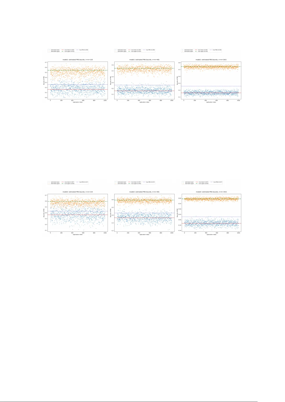
General sample size analysis for probabilities of causation: a delta method approach T ianyuan Cheng 1 , Ruirui Mao 2 , Judea Pearl 3 , and Ang Li 4 1 Department of Statistics, Florida State Uni versity 2 Department of Computer Science, Cornell Uni versity 3 Department of Computer Science, Uni versity of California Los Angeles 4 Department of Computer Science, Florida State Uni versity Abstract Probabilities of causation (PoCs), such as the probability of necessity and sufficiency (PNS), are important tools for decision making but are generally not point identifiable. Ex- isting work has deri ved bounds for these quantities using combinations of experimental and observational data. Howe ver , there is very limited research on sample size analysis, namely , how many e xperimental and observ ational samples are required to achie ve a de- sired margin of error . In this paper, we propose a general sample size framework based on the delta method. Our approach applies to settings in which the target bounds of PoCs can be expressed as finite minima or maxima of linear combinations of experimental and observational probabilities. Through simulation studies, we demonstrate that the proposed sample size calculations lead to stable estimation of these bounds. 1 Intr oduction Probabilities of causation (PoCs) are used in many real-world applications, such as market- ing, law , social science, and health science, especially when decisions depend on whether an action caused an outcome. For e xample, Li and Pearl (2022) introduced a “benefit function” that is a linear combination of PoCs and reflects the payof f or cost of selecting an indi vidual with certain features, with the goal of finding those most likely to show a target behavior . Stott et al. (2004) used it in climate ev ent assignment to quantify how much human influence changes the risk of an extreme ev ent. Mueller and Pearl (2023) argued that PoCs can be used for person- alized decision making, and Li et al. (2020) found that PoCs can be helpful for improving the accuracy of some machine learning methods. W ithout extra assumptions, PoCs are generally not identifiable, so one often works with bounds instead of point values. Using the structural causal model (SCM), Pearl (1999) defined three binary PoCs, including PNS, PN, and PS. T ian and Pearl (2000) deriv ed bounds for these quantities using both experimental and observational information, and later Li and Pearl (2019, 2024) provided formal proofs. Se veral papers studied how to tighten these bounds. For example, 1 Mueller et al. (2021) used covariates and causal structure to narrow the bounds for PNS, and Dawid et al. (2017) used co variates to narro w the bounds for PN. Most of these works implicitly assume that the experimental and observational samples are large enough to estimate the needed probabilities well. Howe ver , there is little work on ho w to choose sample sizes so that the estimated bounds have a desired level of precision. This gap limits the use of the theory in real applications. Li et al. (2022) discussed this issue, b ut focused on a special case for the PNS bound. T o our knowledge, there is still no unified framework that links a tar get error le vel to required experimental and observ ational sample sizes for general PoC bounds. In this paper , we study adequate sample sizes for estimating bounds of PoCs from a general perspecti ve. Our starting point is that many sharp bounds can be written as a finite minimum or maximum of explicit functions of a finite set of probabilities, including experimental prob- abilities such as P ( y x ) and observational probabilities such as P ( x, y ) . For PNS, the bound components are typically linear in these probabilities; for PN and PS, the bound components of- ten take a ratio form. Under mild regularity conditions (e.g., denominators bounded away from zero), the bound components are smooth transformations of the underlying probability vector . The resulting lo wer and upper bounds can still be non-smooth because the y are formed by finite minima or maxima. The fact that the components are smooth but the bounds can be non-smooth leads to dif ferent asymptotic behavior in the two cases, which our results accommodate. Our main contributions are: • W e propose a general sample size framew ork for estimating PoC bound endpoints (i.e., lo wer and upper bounds) with a pre-specified mar gin of error , based on multi v ariate delta- method v ariance approximations for smooth endpoints, and a directional delta method implemented via numerical methods for non-smooth endpoints, following Fang and San- tos (2019). • Our asymptotic results apply whene ver the bound endpoints can be expressed as finite minima or maxima of e xplicit bound components. This covers common forms in the PoC literature and also extends to other bounded causal quantities, including linear combina- tions of PoCs. • W e provide simulation studies sho wing that the proposed sample sizes are stable and suf- ficient in practice, and that they are far less conserv ati ve than e xisting results in the litera- ture. 2 Pr eliminaries In this section, we briefly revie w the definitions of the three aspects of binary causation follo wing Tian and Pearl (2000). Our analysis is based on the counterfactual framew ork within structural causal models (SCMs) as introduced in Pearl (2009). W e denote by Y x = y the counterfactual statement that variable Y would take v alue y if X were set to x . Throughout the paper , we use y x to represent the e vent Y x = y , y x ′ for Y x ′ = y , y ′ x for Y x = y ′ , and y ′ x ′ for Y x ′ = y ′ . Experimental information is summarized through causal quantities such as P ( y x ) , 2 while observ ational information is summarized by joint distributions such as P ( x, y ) . Unless otherwise stated, X denotes the treatment variable and Y denotes the outcome variable. For the following three probabilities of causation, we all assume that X and Y are two binary v ariables in a causal model M . Let x and y stand for the propositions X = true and Y = true, respecti vely , and x ′ and y ′ for their complements. Then we have: Definition 1 (Probability of Necessity (PN)) . The probability of necessity is defined as: PN ≜ P ( Y x ′ = false | X = true , Y = true ) ≜ P ( y ′ x ′ | x, y ) . (1) Definition 2 (Probability of Suf ficiency (PS)) . The probability of sufficienc y is defined as: PS ≜ P ( Y x = true | X = false , Y = false ) ≜ P ( y x | x ′ , y ′ ) . (2) Definition 3 (Probability of Necessity and Suf ficiency (PNS)) . The probability of necessity and suf ficiency is defined as: PNS ≜ P ( Y x = true , Y x ′ = false ) ≜ P ( y x , y ′ x ′ ) . (3) W e also introduce the sharp bounds on the PoCs deriv ed from experimental and observa- tional data in T ian and Pearl (2000), where the bounds are obtained via Balke’ s program in Balke (1995). The bounds are: max        0 , P ( y x ) − P ( y x ′ ) , P ( y ) − P ( y x ′ ) , P ( y x ) − P ( y )        ≤ PNS ≤ min        P ( y x ) , P ( y x ′ ) , P ( x, y ) + P ( x ′ , y ′ ) , P ( y x ) − P ( y x ′ ) + P ( x, y ′ ) + P ( x ′ , y )        . (4) max  0 , P ( y ) − P ( y x ′ ) P ( x, y )  ≤ PN ≤ min  1 , P ( y ′ x ′ ) − P ( x ′ , y ′ ) P ( x, y )  . (5) max  0 , P ( y x ) − P ( y ) P ( x ′ , y ′ )  ≤ PS ≤ min  1 , P ( y x ) − P ( x, y ) P ( x ′ , y ′ )  . (6) 3 Main Results Let θ be a parameter vector that collects all experimental and observ ational probabilities we need. For example, in the setting of the upper bound of (4) we can tak e θ = ( P ( y x ) , P ( y x ′ ) , P ( x, y ) , P ( x ′ , y ′ ) , P ( x, y ′ ) , P ( x ′ , y )) ⊤ . (7) W e first claim that in most scenarios, the bounds of PoCs can be written in the form of a complex linear combination of θ . 3 Lemma 1 (Piece wise-linear and fractional forms of sharp bounds for PoCs) . Consider a struc- tural causal model with finite discrete variables, and focus on the case that X and Y are both binary , i.e. , X has two treatment lev els x, x ′ and Y has two outcome lev els y , y ′ . Let θ ∈ R d collect the observ ational and experimental probabilities used to constrain the model. For a probability of causation Q ∈ { PNS , PN , PS } as defined in Section 2 , let U Q ( θ ) and L Q ( θ ) be its sharp upper and lower bounds ov er all SCMs. Then there exist finite positiv e integers J , K < ∞ , vectors a j , c k ∈ R d and constants b j , d k ∈ R such that U Q ( θ ) = 1 h Q ( θ ) min 1 ≤ j ≤ J { a ⊤ j θ + b j } , L Q ( θ ) = 1 h Q ( θ ) max 1 ≤ k ≤ K { c ⊤ k θ + d k } , (8) where the denominator h Q ( θ ) is defined as: 1. For PNS: h PNS ( θ ) = 1 (reducing to a piecewise-linear form). 2. For PN: h PN ( θ ) = P ( x, y ) , which is a specific component of θ . 3. For PS: h PS ( θ ) = P ( x ′ , y ′ ) , which is a specific component of θ . U Q ( θ ) and L Q ( θ ) are continuous and piecewise-defined functions of θ . They are dif ferentiable at any θ where the optimizer is unique. Pr oof. According to T ian and Pearl (2000), for finite discrete SCMs, sharp bounds for PNS (and the numerators of PN, PS) can be obtained by optimizing a linear functional over the set of latent- type distributions consistent with θ , which is a linear programming (LP) problem. Then, by LP duality and the polyhedral structure of the dual feasible set (see Boyd and V andenber ghe (2004)), the optimal value is a piecewise-linear function of θ and has a finite min or max representation of linear functions a ⊤ θ + b . Lemma 1 giv es a unified form for the sharp bounds: for PNS they are piece wise-linear in θ while for PN and PS they are piecewise linear-fractional due to normalization by P ( x, y ) and P ( x ′ , y ′ ) . In either case, the bound endpoints are piece wise smooth and are differentiable whene ver the acti ve term is unique (optimizer is unique), and thus the inference for the plug-in estimators c U Q = U Q ( b θ ) and c L Q = L Q ( b θ ) reduces to studying piece wise-defined functions of b θ . Next, we establish asymptotic normality and confidence intervals in the regular case where the optimizer is unique. W e first state the setup: let m be the experimental sample size and n be the observ ational sample size. Assume r is the ratio of experimental sample size to observational sample size, i.e. , m/n → r ∈ (0 , ∞ ) . Let θ = ( θ ⊤ e , θ ⊤ o ) ⊤ ∈ R d collect the experimental and observ ational probabilities used in Lemma 1 , with true value θ 0 = ( θ ⊤ e 0 , θ ⊤ o 0 ) ⊤ ∈ R d . Let ˆ θ = ( ˆ θ ⊤ e , ˆ θ ⊤ o ) ⊤ be the plug-in estimator based on the two independent samples. By the multiv ariate central limit theorem (CL T) for multinomial proportions, √ m ( ˆ θ e − θ e 0 ) ⇒ N (0 , Σ e ) , √ n ( ˆ θ o − θ o 0 ) ⇒ N (0 , Σ o ) , (9) and the two limits are independent. Equiv alently , √ n ( ˆ θ − θ 0 ) ⇒ N (0 , Ω r ) , Ω r =  Σ e /r 0 0 Σ o  . (10) 4 Theorem 1. Assume h Q ( θ 0 ) > 0 . Let j ∗ = arg min 1 ≤ j ≤ J { a ⊤ j θ 0 + b j } , k ∗ = arg max 1 ≤ k ≤ K { c ⊤ k θ 0 + d k } , and assume both optimizers are unique with positi ve gaps: ∆ U := min j  = j ∗ ( a ⊤ j θ 0 + b j ) − ( a ⊤ j ∗ θ 0 + b j ∗ ) > 0 , ∆ L := ( c ⊤ k ∗ θ 0 + d k ∗ ) − max k  = k ∗ ( c ⊤ k θ 0 + d k ) > 0 . Suppose √ n ( ˆ θ − θ 0 ) ⇒ N (0 , Ω r ) . Then U Q and L Q are dif ferentiable at θ 0 and √ n ( ˆ U Q − U Q ( θ 0 )) ⇒ N  0 , ∇ U Q ( θ 0 ) ⊤ Ω r ∇ U Q ( θ 0 )  , √ n ( ˆ L Q − L Q ( θ 0 )) ⇒ N  0 , ∇ L Q ( θ 0 ) ⊤ Ω r ∇ L Q ( θ 0 )  . (11) Pr oof. W e pro ve the result for the upper bound U Q only and the proof for lo wer bound is similar . Define g ( θ ) := min 1 ≤ j ≤ J { a ⊤ j θ + b j } , U Q ( θ ) = g ( θ ) h Q ( θ ) . By assumption, the minimizer at θ 0 is unique and has a positi ve gap: ∆ U = min j  = j ∗  a ⊤ j θ 0 + b j  −  a ⊤ j ∗ θ 0 + b j ∗  > 0 . Since each a ⊤ j θ + b j is continuous and the index set is finite, the gap implies that there exist a ϵ > 0 such that for all ∥ θ − θ 0 ∥ ≤ ϵ , the minimizer is j ∗ . Hence g ( θ ) is dif ferentiable at θ 0 . By Danskin’ s theorem (Danskin (2012)), ∇ g ( θ 0 ) = a j ∗ . Because h Q is differentiable at θ 0 and h Q ( θ 0 ) > 0 , it follows that U Q is differentiable at θ 0 with ∇ U Q ( θ 0 ) = h Q ( θ 0 ) ∇ g ( θ 0 ) − g ( θ 0 ) ∇ h Q ( θ 0 ) h Q ( θ 0 ) 2 = h Q ( θ 0 ) a j ∗ − ( a ⊤ j ∗ θ 0 + b j ∗ ) ∇ h Q ( θ 0 ) h Q ( θ 0 ) 2 . No w apply the multiv ariate delta method to the dif ferentiable map θ 7→ U Q ( θ ) at θ 0 : √ n  U Q ( ˆ θ ) − U Q ( θ 0 )  ⇒ N  0 , ∇ U Q ( θ 0 ) ⊤ Ω τ ∇ U Q ( θ 0 )  . (12) Using Theorem 1 we can deri ve a corresponding confidence interv al as follows: 5 Corollary 1. Assume the conditions of Theorem 1 . Let b Ω r be a consistent estimator of Ω r . Define the plug-in v ariance estimators b V U := ∇ U Q ( b θ ) ⊤ b Ω r ∇ U Q ( b θ ) , b V L := ∇ L Q ( b θ ) ⊤ b Ω r ∇ L Q ( b θ ) , and the corresponding standard errors c SE( b U Q ) := q b V U /n, c SE( b L Q ) := q b V L /n. Then, asymptotic (1 − α ) confidence interv als for U Q ( θ 0 ) and L Q ( θ 0 ) are C I U = h b U Q − z 1 − α/ 2 c SE( b U Q ) , b U Q + z 1 − α/ 2 c SE( b U Q ) i , (13) C I L = h b L Q − z 1 − α/ 2 c SE( b L Q ) , b L Q + z 1 − α/ 2 c SE( b L Q ) i , (14) where z 1 − α/ 2 can be found on z-table of standard normal distribution. Pr oof. By Theorem 1, we hav e √ n  b U Q − U Q ( θ 0 )  ⇒ N (0 , V U ) , V U := ∇ U Q ( θ 0 ) ⊤ Ω r ∇ U Q ( θ 0 ) , and similarly √ n  b L Q − L Q ( θ 0 )  ⇒ N (0 , V L ) , V L := ∇ L Q ( θ 0 ) ⊤ Ω r ∇ L Q ( θ 0 ) . Let b Ω r be a consistent estimator of Ω r . Under the uniqueness conditions in Theorem 1, U Q and L Q are dif ferentiable in a neighborhood of θ 0 , hence ∇ U Q ( · ) and ∇ L Q ( · ) are continuous at θ 0 . Since b θ p − → θ 0 , we hav e ∇ U Q ( b θ ) p − → ∇ U Q ( θ 0 ) , ∇ L Q ( b θ ) p − → ∇ L Q ( θ 0 ) . Therefore, by Slutsky’ s theorem (V an der V aart (2000)), b V U := ∇ U Q ( b θ ) ⊤ b Ω r ∇ U Q ( b θ ) p − → V U , b V L := ∇ L Q ( b θ ) ⊤ b Ω r ∇ L Q ( b θ ) p − → V L . Define c SE( b U Q ) = q b V U /n and c SE( b L Q ) = q b V L /n . Then b U Q − U Q ( θ 0 ) c SE( b U Q ) ⇒ N (0 , 1) , b L Q − L Q ( θ 0 ) c SE( b L Q ) ⇒ N (0 , 1) , (15) which gi ves an asymptotic (1 − α ) confidence interv als. When the unique-optimizer assumption in Theorem 1 fails, means that when we hav e mul- tiple activ e constraints, then the bound function may be non-differentiable at θ 0 . In this case we use a directional delta method (see D ¨ umbgen (1993), Fang and Santos (2019)) to deriv e the limiting distribution. The follo wing theorem states the result. 6 Theorem 2. Let U Q ( θ ) and L Q ( θ ) be defined as in equation (8). Assume h Q ( θ 0 ) > 0 and h Q is dif ferentiable at θ 0 . Define the activ e sets as follows: J 0 = arg min j ( a ⊤ j θ 0 + b j ) , K 0 = arg max k ( c ⊤ k θ 0 + d k ) . If √ n  ˆ θ − θ 0  ⇒ Z ∼ N  0 , Ω r  , then √ n  b U Q − U Q ( θ 0 )  ⇒ min j ∈ J 0 g ⊤ U,j Z, √ n  b L Q − L Q ( θ 0 )  ⇒ max k ∈ K 0 g ⊤ L,k Z, (16) where the generalized gradients at θ 0 are g U,j = a j h Q ( θ 0 ) − min ℓ  a ⊤ ℓ θ 0 + b ℓ  h Q ( θ 0 ) 2 ∇ h Q ( θ 0 ) , j ∈ J 0 . g L,k = c k h Q ( θ 0 ) − max ℓ  c ⊤ ℓ θ 0 + d ℓ  h Q ( θ 0 ) 2 ∇ h Q ( θ 0 ) , k ∈ K 0 . Remark 1. If | J 0 | = 1 and | K 0 | = 1 , then the maps U Q ( θ ) and L Q ( θ ) are locally dif ferentiable at θ 0 and the asymptotic results reduce to Theorem 1. If | J 0 | > 1 or | K 0 | > 1 , then in general, the limiting distribution in Theorem 2 is not Gaussian. Instead, it is the distribution of a minimum or maximum of finitely many correlated Gaussian linear forms ev aluated at the Gaussian limit Z ∼ N (0 , Ω r ) . Pr oof. W e pro ve the result for the upper bound U Q only and the proof for lo wer bound is similar . For simplicity , denote m ( θ ) = min j ( a ⊤ j θ + b j ) and r ( θ ) = 1 /h Q ( θ ) so that U ( θ ) = r ( θ ) m ( θ ) . Let J 0 = arg min j ( a ⊤ j θ 0 + b j ) . T ake any sequence t n ↓ 0 and any h n → h , and define θ n = θ 0 + t n h n . Let δ j = ( a ⊤ j θ 0 + b j ) − m ( θ 0 ) ≥ 0 . Then, m ( θ n ) − m ( θ 0 ) t n = min j  a ⊤ j h n + δ j t n  . If j / ∈ J 0 , then δ j > 0 . Since t n ↓ 0 , we have δ j /t n → ∞ , and thus a ⊤ j h n + δ j /t n → ∞ . Therefore, for all suf ficiently large n , the minimum is attained within J 0 , i.e. min j  a ⊤ j h n + δ j t n  = min j ∈ J 0  a ⊤ j h n + δ j t n  . Thus, lim n →∞ m ( θ n ) − m ( θ 0 ) t n = min j ∈ J 0 a ⊤ j h =: m ′ θ 0 ( h ) . By assumption, h Q is differentiable at θ 0 with h Q ( θ 0 ) > 0 , so the map r ( θ ) = 1 /h Q ( θ ) is dif ferentiable at θ 0 and r ′ θ 0 ( h ) = − ∇ h Q ( θ 0 ) ⊤ h h Q ( θ 0 ) 2 . 7 Using U ( θ ) = r ( θ ) m ( θ ) and the decomposition U ( θ n ) − U ( θ 0 ) t n = r ( θ n ) m ( θ n ) − m ( θ 0 ) t n + m ( θ 0 ) r ( θ n ) − r ( θ 0 ) t n +  r ( θ n ) − r ( θ 0 )  m ( θ n ) − m ( θ 0 )  t n , the last term is o (1) because r ( θ n ) − r ( θ 0 ) = O ( t n ) and m ( θ n ) − m ( θ 0 ) = O ( t n ) . Thus, U is Hadamard directionally dif ferentiable at θ 0 with U ′ θ 0 ( h ) = r ( θ 0 ) m ′ θ 0 ( h ) + m ( θ 0 ) r ′ θ 0 ( h ) = 1 h Q ( θ 0 ) min j ∈ J 0 a ⊤ j h − m ( θ 0 ) h Q ( θ 0 ) 2 ∇ h Q ( θ 0 ) ⊤ h. (17) In summary , U ′ θ 0 ( h ) = min j ∈ J 0 g ⊤ U,j h, g U,j = a j h Q ( θ 0 ) − m ( θ 0 ) h Q ( θ 0 ) 2 ∇ h Q ( θ 0 ) , j ∈ J 0 . (18) By the directional delta method (D ¨ umbgen (1993)), √ n  ˆ U − U ( θ 0 )  ⇒ U ′ θ 0 ( Z ) = min j ∈ J 0 g ⊤ U,j Z. (19) Theorem 2 giv es the asymptotic result of ˆ U Q , ˆ L Q , but it is not directly usable in practice because it depends on the unknown activ e set J 0 and K 0 . A natural idea is to use the standard bootstrap, but this fails due to the discontinuity of the directional deriv ative map with respect to θ 0 . T o address this, we apply the numerical delta method of Fang and Santos (2019), which consistently approximates the limit law by numerically ev aluating directional deriv ativ es via finite dif ferences without needing to identify J 0 or K 0 . The corresponding confidence interv als are stated in the following corollary: Corollary 2. Assume the conditions of Theorem 2. Let ˆ Ω r be a consistent estimator of Ω r , and let ϵ n be a sequence satisfying ϵ n → 0 and √ n ϵ n → ∞ . Define the numerical directional deri vati ve statistics for B simulated draws Z ( b ) iid ∼ N (0 , ˆ Ω r ) , b = 1 , . . . , B : T ( b ) U = U Q  ˆ θ + ϵ n Z ( b )  − U Q ( ˆ θ ) ϵ n , T ( b ) L = L Q  ˆ θ + ϵ n Z ( b )  − L Q ( ˆ θ ) ϵ n . Let q U ( τ ) and q L ( τ ) denote the empirical τ -quantiles of { T ( b ) U } and { T ( b ) L } respectiv ely . Then, asymptotic (1 − α ) confidence interv als for U Q ( θ 0 ) and L Q ( θ 0 ) are C I U =  ˆ U Q − q U (1 − α/ 2) √ n , ˆ U Q − q U ( α/ 2) √ n  . (20) C I L =  ˆ L Q − q L (1 − α/ 2) √ n , ˆ L Q − q L ( α/ 2) √ n  . (21) 8 Remark 2. The representation in Lemma 1 is not specific to PoCs. The same form holds for any causal quantity whose sharp bounds can be written as in the form of equation (8) with h ( θ ) > 0 and finite J, K . All asymptotic results in Theorems 1 and 2 continue to hold under the same setup and assumptions. 4 Simulation In this section we run experiments to show that the proposed number of samples provided by Theorems and Corollary in last section are adequate to obtain PoCs within the desired mar gin errors. W e study the bounds for PNS, which is one of the most frequently used PoCs in causal studies. For comparison, we use the same simulation setup as Li et al. (2022), which studies the sharp PNS bound giv en in Section 2. It is trivial to verify that this sharp bound has the form sho wn in Lemma 1 . 4.1 Experiment: estimating PNS bound Follo wing Li et al. (2022), we consider two parameter settings that share the same causal graph in Figure 1 but differ in their coefficients. Here X is a binary treatment with x = 1 , x ′ = 0 , Y is a binary outcome with y = 1 , y ′ = 0 , and Z = ( Z 1 , . . . , Z 20 ) is a set of 20 mutually independent binary covariates. Detailed coefficients are provided in Supplementary materials. Figure 1: The Causal model for PNS bound e xperiment. X and Y are binary , and Z is a set of 20 independent binary confounders. Let U Z i , U X , and U Y be independent Bernoulli exogenous variables. The endogenous co- v ariates are defined as follows: Z i = U Z i , i = 1 , . . . , 20 , and M X = 20 X i =1 a i Z i , M Y = 20 X i =1 b i Z i , where { a i } and { b i } are drawn from Uniform ( − 1 , 1) . Here are the structural equations and we 9 generate ( X , Y ) follo wing these equations with a constant C ∼ Uniform ( − 1 , 1) : X = f X ( M X , U X ) = ( 1 , if M X + U X > 0 . 5 , 0 , otherwise , Y = f Y ( X , M Y , U Y ) = ( 1 , 0 < C X + M Y + U Y < 1 , or 1 < C X + M Y + U Y < 2 , 0 , otherwise . Since all exogenous variables are binary and independent, the population experimental quan- tities ( e.g. , P ( y x ) and P ( y x ′ ) ) and the population observational quantities ( e.g. , P ( x, y ′ ) and P ( x ′ , y ) ) can be computed exactly by summing o ver all configurations of ( U X , U Y , U Z 1 , . . . , U Z 20 ) . For instance, we can compute P ( y x ) = X u X ,u Y , u Z P ( u X ) P ( u Y ) 20 Y i =1 P ( u Z i ) f Y  1 , M Y ( u Z ) , u Y  , and P ( x, y ) = X u X ,u Y , u Z P ( u X ) P ( u Y ) 20 Y i =1 h P ( u Z i ) · f X  M X ( u Z ) , u X  · f Y  f X , M Y ( u Z ) , u Y i , where u Z = ( u Z 1 , . . . , u Z 20 ) and M X ( u Z ) , M Y ( u Z ) denote the corresponding realizations of M X and M Y . W e then generate finite samples under two rules. For the experimental sample of size m , we draw ( U X , U Y , U Z 1 , . . . , U Z 20 ) from their Bernoulli distributions, assign X ∼ Bernoulli(0 . 5) independently of the exogenous variables, and set Y = f Y ( X , M Y , U Y ) . This will giv e i.i.d. experimental pairs ( X, Y ) . Let m ab be the number of experimental samples with ( X = a, Y = b ) and m a · = m a 0 + m a 1 . W e estimate b P ( y x ) = b P ( Y = 1 | X = 1) = m 11 m 1 · , b P ( y x ′ ) = b P ( Y = 1 | X = 0) = m 01 m 0 · . For the observational sample of size n , we again draw the exogenous variables, set X = f X ( M X , U X ) and Y = f Y ( X , M Y , U Y ) , and estimate the required joint probabilities by em- pirical frequencies. Let n ab be the number of observational samples with ( X = a, Y = b ) and n = P a ∈{ 0 , 1 } P b ∈{ 0 , 1 } n ab . For example, b P ( x, y ) = n 11 n , b P ( x, y ′ ) = n 10 n , b P ( x ′ , y ) = n 01 n . These estimated probabilities are then plugged into the bound formulas to get finite-sample bound estimates. Assume the ratio of experimental data to observational data is m/n → r = 1 . Then, Corollary 1 gives adequate experimental size m ≥ 1921 , while result provided in Li et al. (2022) gives m ≥ 6147 . Our method requires only about 31% of the sample size suggested by the existing result. The detailed computation is in Appendix. 10 Figure 2: Scatter plots under different sample sizes for Model 1. Left to right: n = 120 , 481 , 1921 . For both Model 1 and 2, we run 1000 replications, and in each replication, we generate experimental and observ ational samples with sizes n ∈ { 120 , 481 , 1921 } . The results are shown in Figures 2 and 3. When n = 120 , both bounds are highly noisy with large dispersion across replications. Increasing the sample size to n = 481 reduces the noise, but the variance remains relati vely large. When n = 1921 , the adequate size we computed using Corollary 1 , we can see that the estimates become v ery stable, with both the upper and lower bound concentrates tightly around the true bounds, which sho ws a good accuracy and stability . Figure 3: Scatter plots under different sample sizes for Model 2. T op to bottom: n = 120 , 481 , 1921 . W e also examine the relationship between sample size n and the average estimation error , defined as ( \ b ound − true b ound) a veraged over 1000 replications for each model. See Figure 4. Using the target error lev el 0 . 05 (red horizontal line), both Model 1 and Model 2 reach the desired accurac y with sample sizes belo w 300 for both the upper and lo wer bounds (blue/orange curves). The av erage error drops quickly as n increases up to around 500 , which suggests that n = 500 can already work well in practice. This also confirms that the theoretical sample size n = 1921 is more than suf ficient and it represents the adequate size that considers the worst case. W e further in vestigate the relationship between the average estimation error and the sample size n beyond Models 1 and 2. In order to approximate a more general setting, we repeatedly resample the SCM coefficients and rerun the same simulation design as in Model 1 for 20 in- 11 Figure 4: A verage error of estimations VS sample size. Left: Model 1, Right:Model 2 dependent draws. F or each n , we then av erage the estimation error over both the 1000 Monte Carlo replications, and report the resulting curve in Figure 5. It shows that both the upper and lo wer bound estimation errors decrease rapidly as n increases, and in this aggregated experiment the errors con verge e ven faster than in Models 1 and 2. The target error lev el 0 . 05 is reached around 100 , smaller than 500 , which is consistent with our earlier observations. The theoretical sample size n = 1921 remains clearly suf ficient with very small errors for both bounds. In sum- mary , these results suggest that the sample-size selection rule using our Theorems is not tied to a single parameter setting and remains stable and accurate across a range of SCM with dif ferent coef ficients. Figure 5: A verage error with sample size for 20 replicates 5 Discussion The bounds of PoCs are piecewise-defined, and points with multiple optimizers lie on the boundaries between pieces. A way from these boundaries, the optimizer is unique and thus The- orem 1 applies. Since the measure of boundary points are almost zero, we can think Theorem 12 1 holds for most of time. This is supported by our simulations, where the target error is often achie ved with far fewer samples than the theoretical results (around 1 / 4 to 1 / 3 ), suggesting that the acti ve piece is quite stable in a neighborhood of θ 0 . For the non-unique optimizer case in Theorem 2 , one may consider a smooth approxima- tion ( e.g . , Softmin) to enforce differentiability , but this introduces approximation bias and re- quires hyperparameter tuning. For this reason we adopt a conserv ative variance-based approach. Ho wev er , smoothing may still be useful for large-scale repeated ev aluations or gradient-based optimization when near-ties are common and numerical stability is a concern. Most importantly , although we use PoCs (PNS, PN, PS) in binary setup as motiv ating ex- amples, Theorems 1 and 2 apply more broadly . W e discuss two extensions here. First, our proposed method can be directly extended to multi-lev el discrete X and Y , with the same CL T and (directional) delta-method ar guments but at the cost of higher dimension and computational dif ficulty . Second, the same methods can be applied to any bounded causal quantity whose sharp bounds can be written as a finite minimum or maximum of linear (or ratio-type) functions of θ , including linear combinations of PoCs such as the “benefit function” in Li and Pearl (2019). 6 Conclusion W e study the adequate sample size for estimating bounds of PoCs within a desired margin of error . In finite discrete settings, we first show that the bounds can be written as finite minima or maxima of explicit functions of observational and experimental probabilities, including both linear and ratio-type terms. Using this representation, when the bound endpoint is smooth at the true parameter , we use multiv ariate delta-method variance approximations to obtain asymp- totic margins of error; when the endpoint is not smooth due to activ e-set switches in the finite min–max structure, we use a directional delta method and implement it using numerical methods follo wing Fang and Santos (2019). Our asymptotic results apply whenev er the bound endpoints has this finite min max form, which cov ers man y bounds in related literature and also e xtends to other bounded causal quantities, including linear combinations of PoCs. W e also provide simu- lation studies sho wing that the proposed sample sizes are stable and work well in practice, and are less conserv ati ve than e xisting approaches. T o our knowledge, this is the first work providing a general and systematic sample size framework for estimating non-identifiable PoC bounds that handles both smooth and non-smooth endpoints. 13 Refer ences Balke, A. A. (1995). Pr obabilistic counterfactuals: semantics, computation, and applications . Uni versity of California, Los Angeles. Boyd, S. and V andenberghe, L. (2004). Con vex optimization . Cambridge univ ersity press. Danskin, J. M. (2012). The theory of max-min and its application to weapons allocation pr ob- lems , volume 5. Springer Science & Business Media. Dawid, A. P ., Musio, M., and Murtas, R. (2017). The probability of causation. Law , Pr obability and Risk , 16(4):163–179. D ¨ umbgen, L. (1993). On nondif ferentiable functions and the bootstrap. Pr obability Theory and Related F ields , 95(1):125–140. Fang, Z. and Santos, A. (2019). Inference on directionally differentiable functions. The Revie w of Economic Studies , 86(1):377–412. Li, A., J. Chen, S., Qin, J., and Qin, Z. (2020). T raining machine learning models with causal logic. In Companion Pr oceedings of the W eb Confer ence 2020 , pages 557–561. Li, A., Mao, R., and Pearl, J. (2022). Probabilities of causation: Adequate size of experimental and observ ational samples. arXiv pr eprint arXiv:2210.05027 . Li, A. and Pearl, J. (2019). Unit selection based on counterfactual logic. In Pr oceedings of the T wenty-Eighth International J oint Confer ence on Artificial Intelligence . Li, A. and Pearl, J. (2022). Unit selection with causal diagram. In Pr oceedings of the AAAI confer ence on artificial intelligence , v olume 36, pages 5765–5772. Li, A. and Pearl, J. (2024). Probabilities of causation with nonbinary treatment and effect. In Pr oceedings of the AAAI conference on artificial intelligence , volume 38, pages 20465–20472. Mueller , S., Li, A., and Pearl, J. (2021). Causes of effects: Learning individual responses from population data. arXiv pr eprint arXiv:2104.13730 . Mueller , S. and Pearl, J. (2023). Personalized decision making–a conceptual introduction. Jour - nal of Causal Infer ence , 11(1):20220050. Pearl, J. (1999). Probabilities of causation: Three counterfactual interpretations and their iden- tification. Synthese , 121(1-2):93. Pearl, J. (2009). Causality . Cambridge uni versity press. Stott, P . A., Stone, D. A., and Allen, M. R. (2004). Human contribution to the european heatwav e of 2003. Natur e , 432(7017):610–614. T ian, J. and Pearl, J. (2000). Probabilities of causation: Bounds and identification. Annals of Mathematics and Artificial Intelligence , 28(1):287–313. 14 V an der V aart, A. W . (2000). Asymptotic statistics , volume 3. Cambridge univ ersity press. 15 A A ppendix A.1 Calculation of sample size in Experiment 1, PNS bound W e will prove the case of PNS upper bound in (4) only . First, focus on the term P ( y x ) − P ( y x ′ ) + P ( x, y ′ ) + P ( x ′ , y ) . Denote A = P ( y x ) , B = P ( y x ′ ) , C = P ( x, y ′ ) , D = P ( x ′ , y ) , and we can see the A and B come from randomized controlled trial, which can be assumed to be independent with each other , and independent with C and D ; howe ver , C and D come from a multinomial distribution, ( n x,y , n x ′ ,y = n D , n x,y ′ = n C , n x ′ ,y ′ ) ∼ Multinomial ( n ; P ( x, y ) , P ( x ′ , y ) , P ( x, y ′ ) , P ( x ′ , y ′ )) , such that C and D are ne gativ ely correlated. Combine C and D into one ev ent to make C ∪ D ∼ Binomial ( n ; P ( x, y ′ ) + P ( x ′ , y ) =: P C ∪ D ) . Then we have: v ar ( ˆ A − ˆ B + ˆ C + ˆ D ) = v ar ( ˆ A ) + v ar ( ˆ B ) + var \ ( C + D ) = P ( y x )(1 − P ( y x )) m A + P ( y x ′ (1 − P ( y x ′ ) m B + P C ∪ D (1 − P C ∪ D ) n . By AM-GM inequality , p (1 − p ) ≤ 1 / 4 for an y p ∈ [0 , 1] , thus, v ar ( ˆ A − ˆ B + ˆ C + ˆ D ) ≤ 1 4 m A + 1 4 m B + 1 4 n , with constraint m A + m B = m . Assume that m A = m B = m/ 2 , then E r r ( ˆ A − ˆ B + ˆ C + ˆ D ) = z 1 − α/ 2 q v ar ( ˆ A − ˆ B + ˆ C + ˆ D ) ≤ z 1 − α/ 2 2 r 1 m A + 1 m B + 1 n = z 1 − α/ 2 r 1 m + 1 4 n . (22) T aking the error bound to be ϵ = 0 . 05 , then (22) gi ves that m ≥ (1 + 1 4 r )( z 1 − α/ 2 ϵ ) 2 ≈ 1537(1 + 1 4 r ) . (23) When we take m = n , i.e. r = 1 , (22) giv es adequate experimental size n = m ≥ 1921 , which is the sample size in the worst case. A.2 Coefficients of Experiments A.2.1 Model 1 Z i = U Z i , i ∈ { 1 , . . . , 20 } . 16 X = f X ( M X , U X ) = ( 1 , if M X + U X > 0 . 5 , 0 , otherwise. Y = f Y ( X , M Y , U Y ) = ( 1 , if 0 < C X + M Y + U Y < 1 or 1 < C X + M Y + U Y < 2 , 0 , otherwise. U Z 1 ∼ Bernoulli(0 . 352913861526) , U Z 2 ∼ Bernoulli(0 . 460995855543) , U Z 3 ∼ Bernoulli(0 . 331702473392) , U Z 4 ∼ Bernoulli(0 . 885505026779) , U Z 5 ∼ Bernoulli(0 . 017026872706) , U Z 6 ∼ Bernoulli(0 . 380772701708) , U Z 7 ∼ Bernoulli(0 . 028092602705) , U Z 8 ∼ Bernoulli(0 . 220819399962) , U Z 9 ∼ Bernoulli(0 . 617742227477) , U Z 10 ∼ Bernoulli(0 . 981975046713) , U Z 11 ∼ Bernoulli(0 . 142042291381) , U Z 12 ∼ Bernoulli(0 . 833602592350) , U Z 13 ∼ Bernoulli(0 . 882938907115) , U Z 14 ∼ Bernoulli(0 . 542143191999) , U Z 15 ∼ Bernoulli(0 . 085023436884) , U Z 16 ∼ Bernoulli(0 . 645357252864) , U Z 17 ∼ Bernoulli(0 . 863787135134) , U Z 18 ∼ Bernoulli(0 . 460539711624) , U Z 19 ∼ Bernoulli(0 . 314014079207) , U Z 20 ∼ Bernoulli(0 . 685879388218) , U X ∼ Bernoulli(0 . 601680857267) , U Y ∼ Bernoulli(0 . 497668975278) . C = − 0 . 77953605542 . M X = [ Z 1 Z 2 · · · Z 20 ] β X , β X =                                      0 . 259223510143 − 0 . 658140989167 − 0 . 75025831768 0 . 162906462426 0 . 652023463285 − 0 . 0892939586541 0 . 421469107769 − 0 . 443129684766 0 . 802624388789 − 0 . 225740978499 0 . 716621631717 0 . 0650682260309 − 0 . 220690334026 0 . 156355773665 − 0 . 50693672491 − 0 . 707060278115 0 . 418812816935 − 0 . 0822118703986 0 . 769299853833 − 0 . 511585391002                                      . 17 M Y = [ Z 1 Z 2 · · · Z 20 ] β Y , β Y =                                      − 0 . 792867111918 0 . 759967136147 0 . 55437722369 0 . 503970540409 − 0 . 527187144651 0 . 378619988091 0 . 269255196301 0 . 671597043594 0 . 396010142274 0 . 325228576643 0 . 657808327574 0 . 801655023993 0 . 0907679484097 − 0 . 0713852594543 − 0 . 0691046005285 − 0 . 222582013343 − 0 . 848408031595 − 0 . 584285069026 − 0 . 324874831799 0 . 625621583197                                      . A.2.2 Model 2 Z i = U Z i , i ∈ { 1 , . . . , 20 } . X = f X ( M X , U X ) = ( 1 , if M X + U X > 0 . 5 , 0 , otherwise. Y = f Y ( X , M Y , U Y ) = ( 1 , if 0 < C X + M Y + U Y < 1 or 1 < C X + M Y + U Y < 2 , 0 , otherwise. 18 U Z 1 ∼ Bernoulli(0 . 524110233482) , U Z 2 ∼ Bernoulli(0 . 689566064108) , U Z 3 ∼ Bernoulli(0 . 180145428970) , U Z 4 ∼ Bernoulli(0 . 317153536644) , U Z 5 ∼ Bernoulli(0 . 046268153873) , U Z 6 ∼ Bernoulli(0 . 340145244411) , U Z 7 ∼ Bernoulli(0 . 100912238566) , U Z 8 ∼ Bernoulli(0 . 772038172066) , U Z 9 ∼ Bernoulli(0 . 913108434869) , U Z 10 ∼ Bernoulli(0 . 364272290967) , U Z 11 ∼ Bernoulli(0 . 063667554704) , U Z 12 ∼ Bernoulli(0 . 454839320009) , U Z 13 ∼ Bernoulli(0 . 586687215140) , U Z 14 ∼ Bernoulli(0 . 018824647595) , U Z 15 ∼ Bernoulli(0 . 871017316787) , U Z 16 ∼ Bernoulli(0 . 164966968157) , U Z 17 ∼ Bernoulli(0 . 578925020078) , U Z 18 ∼ Bernoulli(0 . 983082980658) , U Z 19 ∼ Bernoulli(0 . 018033993991) , U Z 20 ∼ Bernoulli(0 . 074629121266) , U X ∼ Bernoulli(0 . 29908139311) , U Y ∼ Bernoulli(0 . 9226108109253) . C = 0 . 975140894243 . M X = [ Z 1 Z 2 · · · Z 20 ] β X , β X =                                      0 . 843870221861 0 . 178759296447 − 0 . 372349746729 − 0 . 950904544846 − 0 . 439457721339 − 0 . 725970103834 − 0 . 791203963585 − 0 . 843183562918 − 0 . 68422616618 − 0 . 782051030131 − 0 . 434420454146 − 0 . 445019418094 0 . 751698021555 − 0 . 185984172192 0 . 191948271392 0 . 401334543567 0 . 331387702568 0 . 522595634402 − 0 . 928734581669 0 . 203436441511                                      . 19 M Y = [ Z 1 Z 2 · · · Z 20 ] β Y , β Y =                                      − 0 . 453251661832 0 . 424563325534 0 . 0924810605305 0 . 312680246141 0 . 7676961338 0 . 124337421843 − 0 . 435341306455 0 . 248957751703 − 0 . 161303883519 − 0 . 537653062121 − 0 . 222087991408 0 . 190167775134 − 0 . 788147770713 − 0 . 593030174012 − 0 . 308066297974 0 . 218776507777 − 0 . 751253645088 − 0 . 11151455376 0 . 785227235182 − 0 . 568046522383                                      . 20