Reframing Population-Adjusted Indirect Comparisons as a Transportability Problem: An Estimand-Based Perspective and Implications for Health Technology Assessment

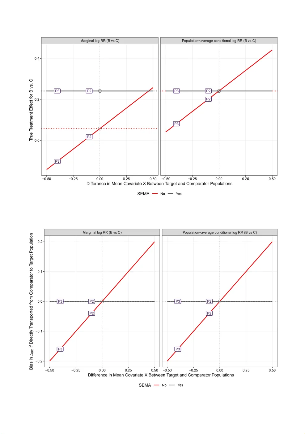
xxx xxx (2026), xx :xx 1–42 P R E P R I N T M A N U S C R I P T R eframing P opulation- A djusted Indirect Com parisons as a T ransportability Problem: An Estimand-Based P erspectiv e and Implications f or Health T echnology Assessment Conor Chandler 1 and Jack Ishak 2 1 PPD, Ther mo Fisher Scientiﬁc, W altham, MA, United States. E-mail: conor.c handler@thermoﬁsher .com . 2 PPD, Ther mo Fisher Scientiﬁc, Montreal, Quebec, Canada. Ke yw ords: transportability; collapsibility; population-adjus ted indirect compar ison; matching-adjus ted indirect compar ison; netw ork meta-anal ysis; health technology assessment Abstract Population-adjus ted indirect comparisons (P AICs) are widel y used to synthesize e vidence when randomized con- trolled trials enroll diﬀerent patient populations and head-to-head compar isons are unav ailable. Although P AICs adjust f or obser v ed population diﬀerences across trials, adjustment alone does not ensure transpor tability of estimated eﬀects to decision-relevant populations f or health technology assessment (HT A). In this paper , w e e xamine and f ormalize transpor tability in P AICs from an estimand-based perspectiv e. W e distinguish conditional and marginal treatment eﬀect estimands and show how transportability depends on eﬀect modiﬁcation, collapsibility , and alignment between the scale of eﬀect modiﬁcation and the eﬀect measure. Using illustrativ e e xamples across continuous, binar y , and time-to-ev ent outcomes, w e demonstrate that e v en when eﬀect modiﬁers are shared across treatments, marginal eﬀects are generall y population-dependent for commonly used non-collapsible measures, including hazard ratios and odds ratios. Conv ersely , collapsible and conditional eﬀects deﬁned on the linear predictor scale e xhibit more fa v orable transpor tability proper ties. W e further sho w that commonly used pairwise P AIC approaches typically identify eﬀects deﬁned in the comparator population and that applying these estimates to other populations entails an additional, often implicit, transport step requir ing fur ther assumptions. This has direct implications f or HT A, where P AIC-der iv ed relativ e eﬀects are routinely applied within cost-eﬀectiv eness and decision models deﬁned f or diﬀerent targ et populations. Our results clar ify when applying P AIC-derived treatment eﬀects to desired targ et populations is justiﬁed, when doing so requires additional assumptions, and when P AIC estimates should instead be inter preted as population- speciﬁc rather than decision-rele vant, supporting more transparent and pr incipled use of indirect evidence in HT A and related decision-making conte xts. 1. Introduction Health technology assessment (HT A) agencies make decisions that determine access to new inter v en- tions across diverse patient populations and real-wor ld healthcare settings. 1-3 Randomized controlled trials (R CT s) are pivotal in HT A, as they are regarded as the gold standard f or establishing causal eﬀects. 4 While R CT s typically achie v e strong inter nal validity , their e xternal validity —the degree to which ﬁndings can be meaningfully applied bey ond the study sample—may be limited. 5-7 R CT s are conducted under controlled conditions and often enroll nar ro w l y deﬁned populations based on strict inclusion and e x clusion cr iteria. 8 Consequentl y , treatment eﬀects observed in R CT s ma y not directly reﬂect outcomes in broader , more heterogeneous patient populations encountered in routine clinical practice—the populations most relev ant to HT A decision-making. 5,9-11 2 Chandler et al. External validity encompasses two inter related but distinct concepts: g eneralizability and transportability . 12,13 Generalizability is deter mined by the extent to which the study sample is repre- sentativ e of the target population. A sample that closel y reﬂects the target population allow s for greater conﬁdence in generalizing the study’ s ﬁndings to that population. 12,13 T ranspor tability ref ers to the abil- ity to transf er a causal eﬀect lear ned in one population (often a study sample) to a diﬀerent external targ et population (e.g., another trial’ s population or a real-w orld population) that may diﬀer in ke y char - acteristics such as baseline risk factors or distributions of eﬀect modiﬁers. 9,12-17 These distinctions ha v e been extensiv ely discussed in the epidemiologic and causal inf erence literature, which has also produced a range of formal statistical framew orks for transporting causal eﬀects across populations. 9,12-14 In the HT A conte xt, transportability is the ke y consideration, since evidence must often be extended from study populations to the real-w orld or jur isdictional populations for which co v erag e and reimbursement decisions are made. 11,18 T ranspor tability issues are especially prominent in indirect treatment comparisons (ITCs), which are widely used in HT A when no head-to-head R CT s directly compare interventions of interest. 19,20 ITCs aim to integ rate and contrast evidence from diﬀerent trials or data sources to estimate relativ e treatment eﬀects—a process sometimes referred to as data fusion. Con v entional ITC methods, including Bucher adjustments and netw ork meta-analy ses (NMAs), assume that all included studies are e x chang eable, meaning that the y represent samples from a common underl ying population. 21-24 U nder this assumption, relativ e treatment eﬀects are inv ariant across studies and can be applied without fur ther adjustment. Ho w e v er , in practice, the populations enrolled in diﬀerent R CT s often diﬀer meaningfully in baseline characteristics and treatment eﬀect modiﬁers, violating the e x chang eability assumption and limiting the validity of unadjusted indirect comparisons. 22,23,25,26 T o address these challeng es, population-adjusted indirect compar isons (P AICs)—suc h as the matching-adjus ted indirect compar ison (MAIC) and simulated treatment compar ison (S TC)—ha v e been dev eloped. 19,27-32 These methods aim to impro v e comparability across studies b y adjusting f or diﬀer - ences in obser v ed eﬀect modiﬁers betw een study populations, typically lev eraging patient-le v el data (PLD) from at least one trial and agg reg ate data from comparator studies. When cor rectly speciﬁed, the y can impro v e the comparability of treatment eﬀect estimates across populations and enhance the relev ance of evidence f or HT A decision-making. 19,27,33 Ho w e v er , the use of P AICs introduces impor tant methodological and practical challeng es. These analy ses rely on strong, often unv er iﬁable assumptions—most notabl y , that all relev ant eﬀect modiﬁers ha v e been measured and that the relationships betw een eﬀect modiﬁers and treatment eﬀects are consis- tent across treatments. 19,27-29,34 Moreo v er , because PLD are rarely av ailable f or all rele vant studies, it is typically not possible to full y test the underl ying assumptions or assess model adequacy , which presents unique challeng es to ensur ing transpor table and unbiased estimates of treatment eﬀects. Impor tantly , ev en when standard P AIC assumptions appear plausible, uncer tainty may remain about whether —and under what conditions—P AIC-derived treatment eﬀects can be v alidly applied to the populations and settings relev ant to HT A. 35 In par ticular , the relationship between adjustment f or population diﬀerences and transportability to new targ et populations is not alwa ys explicit. In this paper , w e e xamine the methodological foundations of transportability in the conte xt of HT A, with a par ticular f ocus on its implications for indirect compar isons. Adopting an es timand-based perspectiv e, we ﬁrst outline the conceptual under pinnings of transportability and its distinction from generalizability , as discussed in the epidemiologic and causal inference literature. 9,12,13,18,36-41 W e then consider ho w assumptions about transpor tability are embedded—e xplicitly or implicitl y—in commonly used ITC and P AIC methods. Finall y , we discuss the factors that inﬂuence transpor tability , including population heterog eneity , measurement of eﬀect modiﬁers, data av ailability , and modeling approaches, and highlight practical considerations f or ensuring that comparativ e eﬀectiv eness evidence is applicable to HT A-rele v ant targ et populations. Although we focus pr imarily on P AICs to motivate concepts, the 3 issues we describe ar ise whenev er treatment eﬀects are transpor ted across populations, including in standard NMAs and cost-eﬀectiv eness models. 2. F oundations of Comparativ e Analy ses 2.1. The Rubin Causal Model Bef ore f ormally deﬁning transpor tability , we ﬁrst introduce the Rubin Causal Model (R CM), which frames causal inference using the concept of potential outcomes. 41,42 W e introduce this notation to ﬁx f oundational concepts and to make e xplicit the estimands underl ying P AIC methods. Let 𝑇 𝑖 denote a dichotomous variable representing the treatment assigned to an individual 𝑖 , where 𝑇 𝑖 = 𝐵 represents assignment to activ e treatment and 𝑇 𝑖 = 𝐴 indicates assignment to the control group (e.g., placebo). Deﬁne 𝑌 𝑡 𝑖 as the potential outcome f or an individual 𝑖 under treatment 𝑡 , where 𝑡 ∈ { 𝐴, 𝐵 } . This framew ork posits that each individual has tw o potential outcomes, one under each treatment arm. 41-44 In reality , only one of these potential outcomes can be obser v ed for an y given individual, corresponding to the treatment that the individual receiv ed in the study ; the other potential outcome is unobserved and is referred to as counter f actual. 43,44 This constitutes the fundamental problem of causal inf erence. 45 The causal eﬀect of the treatment f or an individual 𝑖 is conceptualized as a compar ison between their tw o potential outcomes: 𝜓  𝑌 𝐵 𝑖 , 𝑌 𝐴 𝑖  (1) where 𝜓 ( ·) is a suitable function measur ing the eﬀect of 𝐵 vs. 𝐴 . For instance, this could be a diﬀerence ( 𝑌 𝐵 𝑖 − 𝑌 𝐴 𝑖 ), a ratio ( 𝑌 𝐵 𝑖 / 𝑌 𝐴 𝑖 ), or some transf ormation depending on the outcome scale and interpretation. 2.2. P opulation-aver ag e T reatment Eﬀects In comparativ e eﬀectiv eness researc h, the goal is often to estimate population-a verag e causal eﬀects; 19,35,38 that is, the e xpected diﬀerence in outcomes between treatment 𝐴 and treatment 𝐵 when applied to a speciﬁed population. These population-lev el eﬀects can be expressed in two closely related f or ms: 1. Population-a verag e conditional eﬀects, which av erag e individual-lev el causal contrasts o v er the co v ariate distr ibution; 19,35,46 and 2. Marginal eﬀects, which compare population-a v erage potential outcomes under each treatment, after integrating ov er the cov ar iate distribution. 19,35,46 U nderstanding how these estimands relate—and when they coincide—is essential for later sections on transpor tability , because transpor ting an eﬀect between populations depends on which estimand is targ eted and ho w it depends on the co v ariate distribution. 2.2.1. Causal Estimand vs. St atistical Model T o inter pret conditional and marginal eﬀects, it is impor tant to distinguish between the causal estimand and the statistical model used to estimate it. The causal estimand deﬁnes the target quantity , which is typically a comparison in expected potential outcomes under treatments 𝐴 and 𝐵 : 𝜓  E  𝑌 𝐴  , E  𝑌 𝐵   . The causal estimand is often estimated using a statistical (e.g., regression) model, which provides an empirical representation of the expected outcome given cov ariates: 4 Chandler et al. 𝑔  E  𝑌 𝑡   𝑋   = 𝜂 𝑡 ( 𝑋 ) (2) where 𝑔 ( ·) is the link function mapping the e xpected outcome to the linear predictor scale, and 𝜂 𝑡 ( 𝑋 ) is the linear predictor under treatment 𝑡 . This model provides a conv enient representation f or estimating E { 𝑌 𝑡 | 𝑋 } , which can then be agg reg ated o v er a targ et cov ariate distribution to obtain either conditional or marginal population-av erag e eﬀects. 2.2.2. Conditional vs. Marginal Eﬀects P opulation-a v erag e Conditional Eﬀects A g eneral deﬁnition of a population-av erage conditional eﬀect is the e xpectation (o ver 𝑋 ) of co variate- speciﬁc conditional causal contrasts, possibly after transf ormation: Δ Cond = E 𝑋 h ℎ  E  𝑌 𝐵   𝑋 = 𝑥   − ℎ  E  𝑌 𝐴   𝑋 = 𝑥   i (3.1) Using the regression model in Equation (2), this can be e xpressed as: Δ Cond = E 𝑋 h ℎ  𝑔 − 1 ( 𝜂 𝐵 ( 𝑋 ) )  − ℎ  𝑔 − 1 ( 𝜂 𝐴 ( 𝑋 ) )  i (3.2) Here, 𝑔 ( ·) denotes the link function used in the reg ression model, mapping the e xpected outcome to the linear predictor scale. The function ℎ ( ·) represents a transf ormation deﬁning the eﬀect measure of interest, which ma y be applied on the outcome scale or on a transf ormed outcome scale (e.g., log f or risk ratio, identity f or risk diﬀerence). This broader f ormulation allow s f or the estimation of population- a v erag e conditional eﬀects ev en when the model is ﬁt on one scale (linear predictor via 𝑔 ( ·) ), but the eﬀect measure of interest is deﬁned on a diﬀerent scale (outcome scale via ℎ ( ·) ). For e xample, one may ﬁt a logistic regression (with a logit link, 𝑔 ( ·) ) but wish to estimate a conditional risk ratio, requir ing a log transf ormation (via ℎ ( ·) = log ( ·) ) on predicted probabilities; ho w ev er, if one were to estimate conditional log odds ratios, ℎ ( ·) = 𝑔 ( · ) = logit ( ·) , and thus ℎ  𝑔 − 1 ( ·)  simpliﬁes to the identity function 𝐼 ( ·) . That is, when ℎ ( ·) and 𝑔 ( ·) share the same scale, then Equation (3) simpliﬁes to Equation (4). When the reg ression model and desired eﬀect measure both operate on the linear predictor scale (e.g., logit link used to ﬁt logistic model and estimate log odds ratio), so that ℎ  𝑔 − 1 ( ·)  = 𝐼 ( ·) , population- a v erag e conditional eﬀects can be e xpressed as the e xpected diﬀerences in outcomes f or a patient with a v erag e co variate v alues: Δ Cond = E 𝑋 { 𝜂 𝐵 ( 𝑋 ) − 𝜂 𝐴 ( 𝑋 ) } = E 𝑋 { 𝜂 𝐵 ( 𝑋 ) } − E 𝑋 { 𝜂 𝐴 ( 𝑋 ) } = 𝜂 𝐵 ( 𝑋 ) − 𝜂 𝐴 ( 𝑋 ) (4) where 𝜂 𝑡 represents the modeled linear predictor f or treatment 𝑡 at co variate values 𝑋 . With scale alignment, Equation (3.2) simpliﬁes to Equation (4) because the expectation is linear and a v eraging the co v ariate-speciﬁc eﬀects o v er 𝑋 is equivalent to ev aluating the linear predictor at the mean co v ariate values. This represents the treatment eﬀect for the “av erag e patient ”. Ho w ev er, this inter pretation of the a v erag e conditional eﬀect is somewhat abstract, since the “av erage patient”—sa y 50% male with a mean age of 50 years—does not cor respond to an y real individual in the population. Marginal Eﬀects Marginal eﬀects quantify the chang e in av erag e outcomes across the whole population if ev er y one w ere to receiv e treatment 𝐵 v ersus treatment 𝐴 . 5 Δ Marg = ℎ  E 𝑋  𝑌 𝐵   − ℎ  E 𝑋  𝑌 𝐴   = ℎ  E 𝑋  𝑔 − 1 ( 𝜂 𝐵 ( 𝑋 ) )   − ℎ  E 𝑋  𝑔 − 1 ( 𝜂 𝐴 ( 𝑋 ) )   (5) Because the e xpectation o v er 𝑋 is inside the transformation ℎ ( ·) , marginal eﬀects can depend on the entire co v ariate distribution in w a ys that diﬀer from conditional eﬀects—par ticularl y when 𝑔 ( ·) and ℎ ( ·) are non-linear . When do Conditional and Marginal Eﬀects Coincide? Marginal and conditional eﬀects coincide when equation (5) reduces to the “a v erage patient ” contrast in (4) under restrictiv e conditions, namely when: • The regression model is linear with an identity link (so 𝑔 − 1 ( ·) is linear), and • The eﬀect measure is on the identity scale (i.e., ℎ is the identity function). Outside of this setting, conditional and marginal eﬀects generall y diﬀer , ev en absent conf ounding, because non-linear links and non-identity transf ormations make the estimands depend diﬀerentl y on the co v ariate distr ibution. Later we sho w that f or anchored activ e–activ e indirect comparisons, marginal and conditional eﬀects ma y coincide under additional structural assumptions, ev en when the individual contrasts against a common comparator do not. 2.2.3. Dependence on the P opulation of Study Both conditional and marginal estimands are population-dependent, but the y depend on the population in diﬀerent w a ys. This o v erview f ocuses on marginal treatment eﬀects, as the methods and HT A practices that motivate our central argument most often target marginal estimands. These concepts generalize straightf or w ardly to conditional eﬀects. T o make population dependence e xplicit, let 𝑃 1 denote a source (inde x) tr ial population and 𝑃 2 denote an e xternal target population. The marginal eﬀect in 𝑃 1 is Δ Marg 𝑃 1 = 𝜓  E 𝑃 1  𝑌 𝐵  , E 𝑃 1  𝑌 𝐴   = ℎ  E 𝑃 1  𝑌 𝐵   − ℎ  E 𝑃 1  𝑌 𝐴   (6) Here, E 𝑃 1 { 𝑌 𝑡 } denotes the e xpected potential outcome under treatment 𝑡 in population 𝑃 1 , and ℎ ( ·) is a transf ormation appropr iate f or the eﬀect scale—e.g., a log link when w orking with ratios to transf orm them into an additiv e scale. This additiv e proper ty on the link scale facilitates interpretation and modeling. The marginal treatment eﬀect estimand f or the targ et population is similar ly deﬁned as: Δ Marg 𝑃 2 = 𝜓  E 𝑃 2  𝑌 𝐵  , E 𝑃 2  𝑌 𝐴   = ℎ  E 𝑃 2  𝑌 𝐵   − ℎ  E 𝑃 2  𝑌 𝐴   (7) where E 𝑃 2 { 𝑌 𝑡 } denotes the e xpected potential outcome under treatment 𝑡 in population 𝑃 2 . Diﬀerences between Δ Marg 𝑃 1 and Δ Marg 𝑃 2 arise due to diﬀerences in co variate distributions or eﬀect modiﬁcation across populations, which under pins transpor tability eﬀorts in evidence synthesis. 6 Chandler et al. 3. What is T ransportability? T ranspor tability is concer ned with whether a causal eﬀect lear ned in one population can be validl y applied to a diﬀerent targ et population. 9,13,15 In the HT A context, transportability is often central because evidence is typically g enerated in clinical tr ial populations that diﬀer from the populations for which reimbursement and co v erag e decisions must be made. 18,19,46 W e introduce the notation Δ 𝑃 1 → 𝑃 2 to e xplicitly distinguish the population in which evidence is learned ( 𝑃 1 ) from the population in which the eﬀect is e valuated ( 𝑃 2 ); when 𝑃 1 = 𝑃 2 , this reduces to the usual population-speciﬁc estimand Δ 𝑃 . 3.1. Direct T ransportability (U nadjusted) A treatment eﬀect estimand is directly transportable from a source population 𝑃 1 to a target population 𝑃 2 if the causal eﬀect ev aluated in 𝑃 1 is equal to the causal eﬀect ev aluated in 𝑃 2 . 39 Using the notation introduced in Section 2.2, we wr ite the transported marginal estimand from 𝑃 1 to 𝑃 2 as Δ Marg 𝑃 1 → 𝑃 2 . Direct transportability means that no adjustment is needed because the same estimand holds in both populations. Δ Marg 𝑃 1 → 𝑃 2 = Δ Marg 𝑃 1 = Δ Marg 𝑃 2 (8) The equality in Equation (8) may hold, f or ex ample, when there is no eﬀect modiﬁcation by co v ariates whose dis tributions diﬀer betw een populations, or when the rele v ant eﬀect-modifying co variates ha v e the same distribution in both populations. In many applied settings, how ev er , these conditions are unlikel y to be met. Diﬀerences in baseline characteristics—suc h as ag e, disease sev er ity , or biomarker proﬁles— can induce treatment eﬀect heterogeneity , making unadjusted transport of eﬀects across populations in valid. 3.2. Conditional T ransportability (P opulation-adjusted) When direct transpor tability does not hold, eﬀects may still be transpor table conditionall y . Conditional transportability is in v ok ed when diﬀerences in treatment eﬀects across populations can be e xplained by a set of observed co v ar iates, denoted 𝑋 . 17 In this case, the transpor ted marginal treatment eﬀect from population 𝑃 1 to 𝑃 2 is generall y deﬁned as: Δ Marg 𝑃 1 → 𝑃 2 = 𝜓  𝜇 𝐵 𝑃 1 → 𝑃 2 , 𝜇 𝐴 𝑃 1 → 𝑃 2  (9) where 𝜇 𝑡 𝑃 1 → 𝑃 2 : = E 𝑃 2 { 𝑌 𝑡 } represents the transpor ted expected potential outcome under treatment 𝑡 in the targ et population 𝑃 2 , estimated using information learned from the source population 𝑃 1 . There are generall y tw o types of approaches used to estimate the transpor ted potential outcomes 𝜇 𝑡 𝑃 1 → 𝑃 2 : 1) outcome reg ression modeling and 2) weighting methods. 13 These two approaches underlie commonly used P AIC methods such as S TC (outcome regression) and MAIC (w eighting). 27,28 Both of these statis tical methods account for diﬀerences in 𝑋 betw een populations ( 𝑃 1 ) and ( 𝑃 2 ) and aim to estimate potential outcomes and eﬀects f or treatments 𝐴 and 𝐵 in a ne w population, 𝑃 2 , based on the inf ormation lear ned from the source population 𝑃 1 . In outcome regression, the transpor ted potential outcomes are derived by modeling the conditional outcome given treatment and co variates in the source population 𝑃 1 , and then av eraging predicted outcomes o v er the co v ariate distribution of the target population 𝑃 2 : 𝜇 𝑡 𝑃 1 → 𝑃 2 = E 𝑋 ∼ 𝑃 2  E 𝑃 1 { 𝑌 | 𝑇 = 𝑡 , 𝑋 }  (10) 7 where 𝑋 ∼ 𝑃 2 indicates that 𝑋 are distributed according to the targ et population 𝑃 2 and E 𝑃 1 { 𝑌 | 𝑇 , 𝑋 } represents the tr ue conditional e xpectation of the outcome under treatment 𝑡 , learned from the source trial 𝑃 1 . 47 The outer expectation in Equation (10) is ev aluated by integ rating ov er the co variate distr ibution in the targ et population 𝑃 2 : 𝜇 𝑡 𝑃 1 → 𝑃 2 = ∫ E 𝑃 1 ( 𝑌 | 𝑇 = 𝑡 , 𝑋 = 𝑥 ) | {z } Model for source 𝑓 𝑃 2 ( 𝑥 ) | {z } 𝑋 in targ et 𝑑𝑥 (11) where 𝑓 𝑃 2 ( 𝑋 ) denotes the joint probability density function of co v ariates 𝑋 in the targ et population 𝑃 2 . 9,48 In practice, this is implemented by ﬁtting an outcome regression model on data from 𝑃 1 to estimate the conditional e xpectation of the outcome given treatment and co v ariates. The ﬁtted model is then used to predict the potential outcome under treatment 𝑡 f or individuals in 𝑃 2 , and these predictions are then a v erag ed to obtain an estimate of the transported potential outcome. The integ ral in Equation (11) is typically appro ximated using Monte Carlo integration with obser v ed or simulated data f or the targ et population: 𝜇 𝑡 𝑃 1 → 𝑃 2 = ∫ E 𝑃 1 { 𝑌 | 𝑇 = 𝑡 , 𝑋 = 𝑥 } 𝑓 𝑃 2 ( 𝑥 ) 𝑑𝑥 ≈ 1 𝑛 2 𝑛 2  𝑖 = 1 𝑔 − 1 ( b 𝜂 ( 𝑇 = 𝑡 , 𝑋 = 𝑥 𝑖 2 ) ) (12) where 𝑥 𝑖 2 denotes the cov ariate v ector f or individual 𝑖 in the targ et population of size 𝑛 2 , b 𝜂 ( 𝑇 , 𝑋 ) is the estimated linear predictor from the outcome model, and 𝑔 − 1 ( ·) is the inv erse of the link function f or the regression model. The approach deﬁned in Equations (10) – (12) is commonly ref er red to as g-computation. 9,48-50 Alternativel y , the transpor ted potential outcomes can be estimated using w eighting methods, which aim to adjust the distribution of cov ariates in the source population 𝑃 1 to resemble that of the targ et population 𝑃 2 . 15,51-53 That is, instead of explicitl y modeling the relationship between the outcome and co v ariates, individuals are rew eighted while implicitly preser ving the dependencies observed in the source trial. U nder the weighting frame w ork, the transpor ted potential outcome under treatment 𝑡 is estimated as: 𝜇 𝑡 𝑃 1 → 𝑃 2 = E 𝑃 1  𝑤 𝑃 2 ( 𝑋 ) I ( 𝑇 = 𝑡 ) 𝑌  E 𝑃 1  𝑤 𝑃 2 ( 𝑋 ) I ( 𝑇 = 𝑡 )  (13) where 𝑤 𝑃 2 ( 𝑋 ) are transpor tability weights designed to adjust the source population to align with the targ et population ’ s co v ariate distribution, and I ( 𝑇 = 𝑡 ) is an indicator function f or treatment 𝑡 . W eighting methods are par ticularl y useful when the outcome model is comple x or prone to misspeciﬁcation, but the joint co variate distribution can be estimated reliably . How ev er , they ma y be sensitiv e to e xtreme w eights, especially in settings with limited ov erlap betw een the source and targ et populations. 51,52 Doubly robust methods could also be emplo y ed to transpor t treatment eﬀects. These approaches combine both outcome regression modeling and weighting-based adjustments to provide more reliable estimates of the transported potential outcomes and eﬀects. In par ticular , doubly robust methods oﬀer additional protection agains t model misspeciﬁcation: the estimator remains consistent if either the outcome model or the w eighting model is cor rectl y speciﬁed, though not necessarily both. 54-56 8 Chandler et al. 4. T ransportability in Pairwise P AICs: A Dual Challeng e The transpor tability concepts introduced in Section 3 are particularly consequential in the context of pairwise P AICs, where asymmetr ies in data av ailability require treatment eﬀects to be transpor ted across populations in a structured—but often implicit—manner . This section descr ibes the central methodological challeng e e xamined in this paper. Although we illus trate transpor tability using pairwise P AICs, man y of the same concepts apply to other ITCs (e.g., NMAs) and propag ate f orward into cost-eﬀectiv eness models that use these eﬀect estimates as inputs. In anchored ITCs, PLD are typically a vailable onl y f or the index tr ial comparing a ne w inter v ention 𝐵 with a common comparator 𝐴 , while onl y aggregate data are a v ailable for a comparator tr ial e v aluating an alter nativ e intervention 𝐶 versus 𝐴 (Figure 1). As a result, pair wise P AICs such as MAICs and STCs necessarily treat the index trial as the source population and the comparator tr ial as the target population, yielding relativ e treatment eﬀect estimates deﬁned in the comparator population. 19 Figure 1. Example Netw ork f or Anchored P AIC In v ol ving T w o S tudies Although often described as a single adjustment, pairwise MAICs and STCs inv olv e a two-s tep transport process, each relying on distinct transpor tability assumptions. Step 1: Conditional transport to the comparator population: In the ﬁrst step, the treatment eﬀect f or 𝐵 vs. 𝐴 , Δ 𝐵 𝐴 , is conditionally transpor ted from the index to the comparator study population to estimate 𝐵 vs. 𝐶 ( Δ 𝐵𝐶 ) in the comparator population. MAICs achie v e this b y rew eighting inde x tr ial par ticipants such that the w eighted distr ibution of eﬀect modiﬁers matches the agg reg ate character is tics repor ted for the comparator tr ial. For instance, if the comparator population is composed of 67% lo w -r isk and 33% high-r isk patients, the MAIC weighting ensures the sample from the index tr ial reﬂects the same proportions. This adjustment results in Δ 𝐵 𝐴 ( 𝐴 𝐶 ) , adjusted eﬀect f or 𝐵 vs. 𝐴 in the comparator population. Then, the adjusted eﬀect f or 𝐵 vs. 𝐶 in the comparator (A C) population is estimated on the additiv e scale b y compar ing the adjusted eﬀect for 𝐵 vs. 𝐴 with the reported eﬀect f or 𝐶 vs. 𝐴 : Δ 𝐵𝐶 ( 𝐴 𝐶 ) = Δ 𝐵 𝐴 ( 𝐴 𝐶 ) − Δ 𝐶 𝐴 . STCs instead use outcome reg ression models ﬁtted in the inde x tr ial to predict outcomes under treatment 𝐵 f or co v ar iate proﬁles representativ e of the comparator population. This ﬁrst step relies on the assumption of conditional transpor tability ; that is, that all relev ant eﬀect modiﬁers hav e been correctly identiﬁed and adjus ted f or . 9 Step 2: Implicit direct transport to the decision-rele vant population: In HT A, the comparator trial population is rarely the population of interest. Instead, relative treatment eﬀects are typically applied within cost-eﬀectiv eness models deﬁned f or the index tr ial population or f or broader real-wor ld populations relev ant to reimbursement decisions. Consequentl y , the estimated eﬀect from Step 1 ( Δ 𝐵𝐶 ) is often applied directly to a diﬀerent targ et population—typically , the index trial—implicitly assuming direct transpor tability of the activ e-to-activ e eﬀect, without being f ormally identiﬁed as a second transpor t step in practice. For e xample, Δ 𝐵𝐶 ( 𝐴 𝐶 ) is often an adjusted hazard ratio that is applied to the sur viv al curve f or 𝐵 from the inde x tr ial to der iv e the relative survival of 𝐶 in the index population as par t of health economic model input in HT A. T o justify the second step, analy sts inv oke the shared eﬀect modiﬁer assumption (SEMA), as descr ibed in the N ational Institute for Health and Care Ex cellence (NICE) Decision Support U nit (DSU) T echnical Suppor t Document (TSD) 18. TSD 18 asser ts that the SEMA ensures the ability to transf er inferences of active-to-activ e indirect comparisons (i.e., Δ 𝐵𝐶 ) based on MAIC or STC between studies. 57 The tw o-step nature of pair wise MAICs and STCs creates a dual challeng e (Figure 2). First-order transport (Step 1) must achie v e valid conditional transpor tability from the index to the comparator population by cor rectly adjusting f or all relev ant eﬀect modiﬁers. Second-order transpor t (Step 2) then assumes direct transportability of the resulting eﬀect from the comparator to a diﬀerent target population, relying hea vil y on SEMA. Each stag e introduces its own potential sources of bias. If eﬀect modiﬁers are misspeciﬁed or incompletely reported, Step 1 yields a biased estimate of Δ 𝐵𝐶 ( 𝐴 𝐶 ) . Step 2 relies on SEMA, but we demonstrate in subsequent sections that this assumption ma y not be suﬃcient f or direct transpor tability and may introduce substantial bias. Much of the confusion sur rounding the interpretation of P AIC results in HT A ar ises from the failure to distinguish these tw o transpor t s teps and their distinct assumptions. Figure 2. T wo-s tep Process to T ranspor ting Eﬀects in Pairwise MAICs and STCs 10 Chandler et al. 5. Central Role of the Shared Eﬀect Modiﬁer Assumption In P AICs, SEMA comprises two ke y conditions when compar ing a set of active treatments (e.g., 𝐵 and 𝐶 ) relativ e to a common comparator ( 𝐴 ): (1) the same set of co v ariates function as eﬀect modiﬁers; and (2) the strength and direction of each eﬀect modiﬁer’ s impact on the treatment eﬀect are identical across all active treatments. 19,28,46 SEMA pla y s a pivotal role in P AICs, as it is often inv oked to facilitate transporting eﬀects across populations. 46,57,58 When SEMA holds, cur rent guidance sugges ts that eﬀect modiﬁers “cancel out” for activ e-to-activ e indirect compar isons (e.g., 𝐵 vs. 𝐶 ), thereby enabling the direct transpor tability of Δ 𝐵𝐶 to any population, including the inde x study . 28,57,58 Historically , both MAICs and STCs ha v e relied on SEMA to justify transpor ting treatment eﬀects f or active-to-activ e comparisons (e.g., 𝐵 vs. 𝐶 ) from the comparator population to the desired target population (e.g., inde x study). 28,57,58 The impor tance of SEMA in the conte xt of transpor tability in P AICs is underscored in cur rent guidance from ke y HT A bodies. NICE DSU TSD 18 states the f ollo wing: “[. . . ] if the shared eﬀect modiﬁer assumption holds for tr eatments B and C, then the estimated marginal relativ e treatment eﬀect (whether obtained using anc hor ed or unanchor ed MAIC/STC) will be applicable to any population. ” 57 Similarl y , the HT A coordination group (CG), which is responsible f or o v erseeing the Joint Clinical Assessments (JC As) aimed at ev aluating the clinical eﬀectiveness of new health technologies across the European U nion (EU), supports NICE’ s position. The HT A CG has concluded that it is feasible and appropriate to directl y transpor t relativ e eﬀect estimates obtained from MAIC or STC to the desired targ et population when SEMA is met, stating: “When this [SEMA] holds, the relativ e eﬀect betw een any pair of tr eatments in this set [of activ e treatments] will be the same in any population, whic h means that tr eatment eﬀects obtained from population-adjusted indirect comparisons [MAICs and STCs] can be transposed to the population of the source [index] trial or indeed any ot her r elevant population” 58 Despite its central role in HT A guidance, SEMA alone does not guarantee direct transpor tability of marginal treatment eﬀects. 46 In Sections 6 and 7 we provide both theoretical arguments and present illustrativ e e xamples to clarify that, in g eneral, SEMA is not alw a y s suﬃcient to guarantee direct transportability of Δ 𝐵𝐶 . If SEMA is met and both eﬀect modiﬁcation and eﬀect measures are modeled on the linear predictor scale (Section 6.3), then population-av erage conditional eﬀects are directly transportable. For marginal eﬀects, only cer tain measures (e.g., mean diﬀerences, r isk ratio), which are said to be collapsible (Section 6.2), are directl y transpor table if these assumptions are met; how ev er , marginal eﬀects for measures that are non-collapsible, including odds ratios and hazard ratios—which are the mos t common measures compared in practice—are not directly transpor table, e v en when SEMA holds. Theref ore, the cur rent guidance 57,58 is not suﬃcient, as SEMA is not proper justiﬁcation f or transporting eﬀects in MAICs and STCs, as these methods typically targ et marginal estimands rather than conditional estimands. 6. Be y ond SEMA: Estimands and Conceptual F oundations T ranspor tability in P AICs depends on both the estimand that deﬁnes the causal contrast of interest and the analytic conditions under which the treatment eﬀect can be v alidly transpor ted across study populations. W e ﬁrst distinguish betw een conditional and marginal estimands (Section 6.1), then discuss collapsibility (Section 6.2) and the cor respondence betw een the scale of eﬀect modiﬁcation and the eﬀect measure (Section 6.3), before summarizing the joint conditions for direct transpor tability (Section 6.4). T ogether with SEMA, these concepts collectivel y deﬁne the theoretical boundar y betw een directly and conditionally transpor table relativ e eﬀects in pairwise P AICs. Figure 3 pro vides a high-lev el decision frame w ork f or deter mining when unadjusted indirect com- parisons (e.g., NMA or Bucher ’ s method) are suﬃcient and when population-adjusted approaches are required to address transpor tability concer ns arising from imbalances in eﬀect modiﬁers or prognostic factors. 11 6.1. T ype of T arget Estimand: Conditional vs. Marginal As discussed in Section 2.2, the distinctions betw een conditional and marginal estimands are central to P AICs, which seek to estimate treatment eﬀects that are valid in a target population when onl y agg reg ate data are av ailable from comparator tr ials. Diﬀerent P AIC approaches target diﬀerent estimands. 19,46 MAIC targets marginal eﬀects by construction. STC and multilev el network meta-regression (ML - NMR) can targ et either population-a v erag e conditional or marginal eﬀects, depending on the model and post-processing steps. How e v er , STCs are often constrained in practice by the f or m of the eﬀect measure reported in the comparator study , which is typically marginal. 19,46 Sections 5, 6.2, and 6.3 ex amine ho w SEMA, collapsibility , and the alignment between the model scale and the desired eﬀect measure inﬂuence the transportability proper ties of the estimand being targ eted. When both the model link 𝑔 ( ·) and eﬀect scale ℎ ( ·) are identity functions (i.e., the estimand concerns diﬀerences in mean outcomes), the marginal and conditional eﬀect at the av erage co variate values coincide, and direct transpor tability is f easible under SEMA (Section 6.2). The mathematical intricacies of marginal eﬀects, which inv ol v e translating estimates across multiple diﬀerent scales, via ℎ ( ·) and 𝑔 ( ·) , can complicate transpor tability . In practice, it ma y be comparativ ely easier to achie v e transportability of conditional eﬀects in indirect comparisons, par ticular ly when eﬀect modiﬁcation and eﬀect measurement are e xpressed on compatible scales (Section 6.3). 6.2. Collapsibility and Its Role in T ransportability Collapsibility descr ibes how statistical measures behav e when av eraging across subgroups—par ticularl y , whether a measure computed in subgroups can be “collapsed” to give the same result in the o v erall population. 35,59,60 More precisely , collapsibility refers to the proper ty whereby marginal eﬀects can be e xpressed as a weighted av erage of conditional eﬀects. 35,59,60 Direct collapsibility is a special case in which the population-av erage conditional eﬀect and marginal eﬀect are mathematicall y equivalent (i.e., the marginal eﬀect coincides with an av erag e of conditional eﬀects using population-representative w eights). 35,60 Non-collapsibility refers to measures that are not collapsible. 35,59,60 In the causal inf erence literature, collapsibility is con v entionall y discussed as an intr insic property of an eﬀect measure f or a direct, within-population compar ison (e.g., Δ 𝐵 𝐴 ). In anchored ITCs, ho w e v er , the estimand of interes t is an anc hored active–activ e contrast ( Δ 𝐵𝐶 = Δ 𝐵 𝐴 − Δ 𝐶 𝐴 ), constructed indirectly via a common comparator and therefore structurally diﬀerent from such within-population compar isons. As a result, the collapsibility properties rele vant f or transpor tability depend not only on the eﬀect measure, but also on how the anchored contrast is constr ucted. If the individual contrasts Δ 𝐵 𝐴 and Δ 𝐶 𝐴 are directly collapsible, then Δ 𝐵𝐶 = Δ 𝐵 𝐴 − Δ 𝐶 𝐴 is also directly collapsible. More subtly , ev en when the underlying Δ 𝐵 𝐴 and Δ 𝐶 𝐴 contrasts are collapsible but not directly collapsible, Δ 𝐵𝐶 e xhibits direct collapsibility as an induced proper ty of the anchored contrast under SEMA and scale alignment, contrar y to what w ould be expected based on the collapsibility proper ties of the individual contrasts alone. In this setting, eﬀect- modiﬁcation ter ms cancel in the activ e–activ e contrast, yielding marginal–conditional equiv alence f or Δ 𝐵𝐶 . A f ormal proof of these results is provided in Appendix B. T ranspor tability of marginal eﬀects depends on whether the chosen measure is collapsible and on what aspects of the cov ariate dis tribution it depends upon. A recent simulation s tudy b y Remiro- Azócar empir ically demonstrates that both eﬀect modiﬁers and purely prognostic factors may modify marginal eﬀects f or measures that are not directly collapsible. 35 In other words, a prognostic factor on the conditional scale may be a modiﬁer of the marginal eﬀect measure. Thus, successfull y transporting these types of marginal eﬀects requires adjusting f or the entire joint distr ibution of purely prognostic factors and treatment eﬀect modiﬁers, which is often challenging to fully address due to the limited data a vailable for comparator studies (e.g., unkno wn correlations in comparator studies). These ﬁndings highlight a critical distinction in transpor tability : whether an eﬀect measure f or marginal eﬀects depends on (i) marginal cov ariate means (or more g enerally , moments) of eﬀect modiﬁers or (ii) the full joint 12 Chandler et al. co v ariate distribution of eﬀect modiﬁers and prognostic f actors. Non-collapsible measures generall y depend on the full joint co v ariate distribution, including prognostic f actors, making them more diﬃcult to reliably transpor t across study populations. Further more, Remiro- Azócar concludes that directl y collapsible eﬀect measures “facilitate the transportability of mar ginal eﬀects betw een studies, ” as the y onl y depend on marginal cov ar iate moments—typically the cov ariate means—of eﬀect modiﬁers but not prognostic factors. 35 In this paper w e present simulated ex amples to fur ther clar ify that directl y collapsible eﬀect measures depend on marginal cov ariate moments if and only if eﬀect modiﬁers and the eﬀect measure both operate on the linear predictor scale. Ho we ver , if the scales diﬀer , ev en directly collapsible measures—such as the risk diﬀerence when der iv ed from a logit model—generall y depend on the full joint cov ariate distribution, including both eﬀect modiﬁers and purely prognostic f actors (Section 6.3). Collapsibility and transportability are sometimes conﬂated. The distinction betw een collapsibility as a within-population property and transpor tability as a cross-population proper ty of an estimand is discussed in more detail in Appendix D. 6.3. Scale of Eﬀect Modiﬁcation and Correspondence with Eﬀect Measure When consider ing the transportability properties of an eﬀect, it is cr ucial to understand the relationship betw een the scale of eﬀect modiﬁcation (e.g., additive or multiplicativ e) and the eﬀect measure (e.g., risk diﬀerence, risk ratio, odds ratio). For instance, whether an eﬀect Δ 𝐵𝐶 is directly transpor table depends on the scale on which eﬀect modiﬁcation is modeled and how it cor responds to the chosen eﬀect measure. An eﬀect may be directly transpor table only if both the eﬀect modiﬁcation and the eﬀect measure operate on the linear predictor scale (i.e., ℎ ◦ 𝑔 − 1 = 𝐼 ). Here, the linear predictor scale ref ers to a modeling frame w ork in which the eﬀects of treatment, prognostic factors, and eﬀect modiﬁers are assumed to be additiv e, resulting in a linear relationship. These considerations highlight that direct transportability ultimately requires inv ariance of the estimand on the linear predictor scale to chang es in the co v ariate dis tr ibution across populations. How this inv ariance ar ises—through SEMA, collapsibility , and scale alignment—and under what conditions it holds is summarized in Section 6.4. 6.4. Conditions f or Direct T ransportability T ranspor tability in MAICs and STCs depends on the interdependent concepts discussed in Sections 4, 5, and 6. T ogether , these concepts collectiv ely deﬁne the theoretical boundary between directly and conditionally transpor table relativ e eﬀects in pairwise analy ses. W e illustrate in Section 7 that marginal indirect eﬀects are directly transportable only if the f ollo wing conditions are met: (i) SEMA holds; (ii) both the eﬀect modiﬁers and the eﬀect measure operate on the same linear predictor scale; and (iii) the eﬀect measure is collapsible. When these conditions are jointl y satisﬁed, the resulting marginal estimand Δ 𝐵𝐶 is induced to exhibit marginal–conditional equiv alence (analogous to direct collapsibility) and is directl y transpor table, meaning it is inv ariant to changes in the co v ariate distr ibution across populations. In contrast, population-a v erag e conditional eﬀects are directly transportable if SEMA is met and eﬀect modiﬁers and the eﬀect measure both operate on the linear predictor scale—regardless of whether the measure is collapsible. In both cases, direct transpor tability reﬂects a property of the anchored estimand under structural assumptions, rather than an intr insic f eature of P AIC methods or eﬀect measures. N otably , conditional linearity of the treatment eﬀect in the co v ariates is not required f or direct transpor tability . The formal conditions under which conditional and marginal activ e-to-activ e contrasts are directly transportable are stated as Propositions A1–A2 and prov ed in Appendix A. A more comprehensive summary of the requirements f or direct transpor tability is pro vided in Section 8. Figure 4 synthesizes these considerations into a decision framew ork showing ho w estimand choice (conditional vs marginal), 13 collapsibility of the eﬀect measure, scale alignment, and SEMA jointl y deter mine whether P AIC-derived treatment eﬀects are directly transpor table or population-speciﬁc. Figure 3. Decision Frame w ork f or Deter mining When Unadjus ted NMAs Identify a T ransportable T reatment Eﬀect Estimand and When P AICs Are Required Figure 3 focuses on direct transpor tability of unadjusted indirect compar isons of Δ 𝐵𝐶 ; population invariance of marginal estimands may arise either from the absence of eﬀect modiﬁcation or, in special cases, from str uctural proper ties of the estimand (e.g., collapsibility on a compatible scale). When these conditions are not met, the issue is not merely failed transpor tability but the absence of a single marginal estimand shared across studies, and unadjusted NMAs combine population-dependent eﬀects rather than identifying a common marginal estimand. Figure 4. Frame w ork f or Selecting P AIC Methods and Assessing T ranspor tability of T reatment Eﬀects U nder Estimand Choice, Collapsibility , and SEMA 14 Chandler et al. Even when the SEMA holds, direct transportability of Δ 𝐵𝐶 across populations depends on the target estimand (conditional vs marginal), the collapsibility of the eﬀect measure, and alignment between the scale of eﬀect modiﬁcation and the eﬀect measure. For commonly used non- collapsible marginal measures (e.g., hazard ratios), MAIC and STC estimates are generall y valid only in the comparator population. ML -NMR may support conditional transport to relev ant target populations, but this relies on additional modeling assumptions and does not, in g eneral, guarantee direct transportability of marginal eﬀects. 7. Illustrativ e Examples of T wo-step T ransportability in MAICs/ST Cs In this section, we use illustrativ e simulations to ev aluate the second step in the tw o-step transpor t process often implicit in MAICs and STCs—namel y , the application of an active-to-activ e indirect comparison Δ 𝐵𝐶 ( 𝐴 𝐶 ) , identiﬁed in the comparator population via conditional transport (Step 1), to a diﬀerent decision-relev ant population. Pr ior simulation studies hav e pr imarily e xamined the statistical performance of MAICs and STCs f or Step 1 under model misspeciﬁcation, limited ov er lap, and ﬁnite- sample constraints. 34,35,49,61-66 More recently , Remiro- Azócar highlighted that Step 1 can be particularly challenging f or non-directly -collapsible marginal estimands due to their dependence on the full joint co v ariate distribution. 18,35 Here, how ev er , w e deliberately isolate Step 2, which is often o v erlook ed in practice. Step 1 is treated as successful by assuming that Δ 𝐵𝐶 ( 𝐴 𝐶 ) is estimated without bias, and w e e xamine whether this estimate remains valid when directly transpor ted to populations with diﬀerent co v ariate distributions. Framed in estimand terms, this amounts to testing whether Δ 𝐵𝐶 is in variant to chang es in the target population ’ s cov ariate distribution, as is often implicitly assumed under SEMA in practice. W e illustrate these transpor tability proper ties across ﬁv e diﬀerent eﬀect measures: 1. Mean diﬀerence, estimated via linear reg ression 2. Log odds ratio, estimated via logistic regression 3. Log risk ratio, estimated via log-binomial regression 4. Diﬀerence in restricted mean survival time (RMST), estimated using W eibull regression 15 5. Log ratio of RMST , also estimated using W eibull regression For each analy sis, w e speciﬁed a regression model character izing the true relative eﬀects of 𝐵 vs. 𝐴 and 𝐶 vs. 𝐴 , adjusting for a single cov ariate 𝑋 that is both an eﬀect modiﬁer and prognostic factor (i.e., the true outcome model). 𝑋 w as unif ormly distributed with mean 𝜇 𝑋 ( 𝑃 ) (which is speciﬁc to a given population P) and a ﬁxed rang e of 2: 𝑋 ∼ U nif ( 𝜇 𝑋 ( 𝑃 ) , range = 2 ) . This cor responds to the type of outcome regression model commonly estimated in S TC and ML -NMR. 𝑋 was centered at the mean of the comparator population. W e simulate 21 populations with 𝜇 𝑋 ( 𝑃 ) values ranging from -0.5 to 0.5 in increments of 0.05, with each population compr ising one million individuals. T o inv es tigate the transpor tability properties of eac h eﬀect measure, we derive mar ginal and population-a v erag e conditional eﬀects for 𝐵 vs. 𝐶 in each simulated population. The relative eﬀect in the comparator population (where 𝜇 𝑋 = 0 ) represents the adjusted result that w ould be estimated via MAIC or STC under the conditional transpor tability assumption. Equality of the eﬀect estimate across all 21 populations w ould indicate direct transportability of Δ 𝐵𝐶 (i.e., Step 2 in MAICs and STCs). 7.1. Mean Diﬀerence The tr ue outcome model f or a continuous outcome 𝑌 | 𝑋 ∼ Norm ( 𝜂 𝑘 ( 𝑃 ) , 𝜎 2 ) with the identity link function (i.e., 𝑔 ( 𝐸 { 𝑌 | 𝑋 }) = 𝐸 { 𝑌 | 𝑋 } ) was deﬁned as E { 𝑌 | 𝑋 } = 𝜂 𝑘 ( 𝑃 ) = 𝛽 0 + 𝑥 𝑖 𝑘 ( 𝑃 ) 𝛽 1 + 𝑥 𝑖 𝑘 ( 𝑃 ) 𝛽 2 , 𝑘 + 𝛾 𝑘 (14) where 𝑘 ∈ { 𝐴 , 𝐵, 𝐶 } represents treatment group, 𝛽 0 = 20 is the intercept (common baseline r isk across all populations), 𝛽 1 = 10 is the prognostic eﬀect of 𝑋 , 𝛽 2 , 𝑘 represents an interaction ter m f or eﬀect modiﬁcation (with 𝛽 2 , 𝐴 = 0 b y deﬁnition), and 𝛾 𝑘 is the baseline treatment eﬀect, with 𝛾 𝐵 = 10 and 𝛾 𝐶 = 5 . W e consider two scenarios regarding eﬀect modiﬁcation. Under the SEMA, eﬀect modiﬁcation is assumed to be shared across both activ e treatments, suc h that 𝛽 2 , 𝐵 = 𝛽 2 , 𝐶 = 2 . In contrast, under the no-SEMA scenario, eﬀect modiﬁcation is treatment-speciﬁc, with 𝛽 2 , 𝐵 = 2 and 𝛽 2 , 𝐶 = − 4 . Figure 5 displa ys the bias incur red when directly transporting marginal and population-av erage mean diﬀerences for 𝐵 vs. 𝐶 from the comparator population (identiﬁed in Step 1 of an MAIC/STC) to target populations with diﬀering cov ariate distributions (Step 2). In the linear setting, population-av erage conditional and marginal mean diﬀerences are mathematically equivalent (i.e., direct collapsibility), and thus are represented b y the same line. The vertical line at 𝜇 𝑋 ( 𝐴𝐶 ) = 0 denotes the comparator population, in which Δ 𝐵𝐶 ( 𝐴 𝐶 ) is identiﬁed via MAIC or STC. When SEMA holds, Δ 𝐵𝐶 is inv ar iant across all populations, resulting in zero transpor t bias across all values of 𝜇 𝑋 ( 𝑃 ) ; that is, the comparator -population estimate Δ 𝐵𝐶 ( 𝐴 𝐶 ) is unaﬀected by shifts in the distribution of 𝑋 and can be directly transported to an y external targ et population under SEMA. How e v er , in the absence of SEMA, the bias increases linearl y as the mean of 𝑋 div erg es from the comparator population, implying that Δ 𝐵𝐶 is not directly transpor table across populations. T o illustrate this more concretely , we ex amine two hypothetical targ et populations (of the 21 simulated to dra w the ﬁgures): 𝑃 2 with 𝜇 𝑋 = − 0 . 1 and 𝑃 3 with 𝜇 𝑋 = − 0 . 4 . W e compare the adjusted eﬀect in the comparator population (central reference point, 𝑃 1 ) with the tr ue eﬀect in 𝑃 2 and 𝑃 3 (i.e., ﬂagged points along the red line). Under the no-SEMA scenario, the div erg ence betw een the adjusted eﬀect in the comparator population and tr ue eﬀect in the targ et grow s as the mean of 𝑋 shifts fur ther from zero (i.e., the tr ue eﬀect in 𝑃 2 is closer to the comparator population than 𝑃 3 ). In general, the magnitude of this discrepancy depends on both the strength of the eﬀect modiﬁcation f or 𝐵 v s. 𝐶 , calculated as 𝛽 2 , 𝐵 − 𝛽 2 , 𝐶 , and the e xtent of o v er lap in joint co variate distributions betw een populations. Figure 5. Bias in Conditional and Marginal Mean Diﬀerences Under Direct T ranspor tability 16 Chandler et al. Bias is shown as a function of the diﬀerence in the mean of co variate 𝑋 between the target and comparator populations. The vertical dashed line denotes the comparator population ( 𝜇 𝑋 ( 𝐴𝐶 ) = 0 ), in which the P AIC estimand Δ 𝐵𝐶 ( 𝐴 𝐶 ) is identiﬁed. A ﬂat line indicates direct transpor tability (i.e., zero Step-2 transport bias), as is observed when SEMA holds. Any line or cur v e that is not completely ﬂat indicates that bias is induced in Step 2 by directly transpor ting the eﬀect der iv ed in the comparator population to other target populations. 7.2. Log Odds Ratio and Risk Ratio Ne xt, we consider a logistic reg ression model for a binar y outcome. The general model structure is identical to that in the pre vious section, but the link function is logit, and the conditional distr ibution of the outcome is 𝑌 | 𝑋 ∼ Binomial  logit − 1 ( 𝜂 𝑘 ( 𝑃 ) )  . W e assume parameters 𝛽 0 = 0 , 𝛽 1 = − 1 , 𝛾 𝐵 = − 3 , 𝛾 𝐶 = − 4 . U nder the SEMA, we set 𝛽 2 , 𝐵 = 𝛽 2 , 𝐶 = − 3 , while under the alter nativ e scenar io without SEMA, 𝛽 2 , 𝐵 = − 3 and 𝛽 2 , 𝐶 = − 4 . Figure 6 display s the bias incur red when directly transpor ting conditional and marginal log odds ratios f or 𝐵 vs. 𝐶 from the comparator population to targ et populations with diﬀer ing co v ariate distributions. For the conditional log odds ratio (left panel), the general pattern mirrors that observed f or mean diﬀerences: when SEMA holds, the conditional log odds ratio f or 𝐵 vs. 𝐶 is inv ariant across populations, resulting in zero transpor t bias. When SEMA is violated, transpor t bias increases linearl y as the mean of X div erg es from that of the comparator population, reﬂecting treatment-speciﬁc eﬀect modiﬁcation. In contrast, f or the marginal log odds ratio (r ight panel), transport bias occurs and varies with the co v ariate distribution ev en when SEMA holds. This reﬂects the non-collapsibility proper ty of the (log) odds ratio. As marginal log odds ratios av erag e o v er the cov ariate distribution, the y depend nonlinear ly on both the conditional outcome model and the joint distribution of co v ariates. As a result, marginal log odds ratios are not directly transportable, regardless of whether SEMA is satisﬁed. This e xample highlights a k e y distinction between conditional and mar ginal estimands: while conditional eﬀects deﬁned on the model’ s linear predictor scale may be directly transpor table under SEMA, marginal eﬀects f or non-collapsible measures g enerall y are not. Figure 6. Bias in Conditional and Marginal Log Odds Ratios Under Direct T ranspor tability 17 Bias is shown as a function of the diﬀerence in the mean of co variate 𝑋 between the target and comparator populations. The vertical dashed line denotes the comparator population, in which the P AIC estimand is identiﬁed. Left panel: conditional log odds ratios exhibit zero transpor t bias under SEMA, indicating direct transportability , but incur bias when SEMA is violated. Right panel: marginal log odds ratios exhibit population dependence ev en when SEMA holds, reﬂecting non-collapsibility and failure of Step-2 direct transpor tability . W e replicated the str ucture of the log odds ratio e xample using a log-link model to generate a binary outcome with the same co v ariate structure and patter n of eﬀect modiﬁcation, but targ eting the log r isk ratio instead of the log odds ratio (details in Appendix C). U nder this log-r isk model, the marginal log risk ratio f or 𝐵 vs. 𝐶 w as inv ariant across populations when SEMA held, mir roring the mean-diﬀerence e xample (Figure 5). This contrasts with the log odds ratio e xample, where non-collapsibility induces population dependence ev en when SEMA holds. This illustrates that despite both being multiplicativ e measures, r isk ratios and odds ratios hav e fundamentally diﬀerent transportability properties. This result illustrates the contrast-induced direct collapsibility descr ibed in Section 6.2, under which the anchored 𝐵 vs. 𝐶 log r isk ratio is in variant across populations when SEMA holds on the log link scale. 7.3. RMS T Diﬀerences and Ratios Although hazard ratios are commonl y repor ted f or survival outcomes, marginal hazard ratios are inherently population-dependent due to non-collapsibility; analogous to the patterns for the odds ratio sho wn in Figure 6, conditional hazard ratios f or Δ 𝐵𝐶 are in v ariant across populations under SEMA, whereas marginal hazard ratios are not (T able 1), and may also vary ov er time. RMST -based measures are often adv ocated as alternatives to hazard ratios, as they are collapsible and clinicall y interpretable. In the ﬁnal scenario, w e ex amine the proper ties of RMST -based measures using a parametric W eibull survival model. The survival function f or treatment ar m 𝑘 in population 𝑃 is deﬁned as 𝑆 𝑘 ( 𝑃 ) ( 𝑡 | 𝑥 ) = e xp  − 𝑡 𝜈 e xp  𝜂 𝑘 ( 𝑃 ) ( 𝑥 )   (15) 18 Chandler et al. where the shape parameter 𝜈 = 1 . 5 is assumed to be common across populations, and 𝜂 𝑘 ( 𝑃 ) f ollo w s the same general speciﬁcation as in Equation (14). The model includes a ﬁx ed intercept 𝛽 0 = − 1 (i.e., common baseline risk), prognostic coeﬃcient 𝛽 1 = log ( 0 . 25 ) , and baseline treatment eﬀects 𝛾 𝐵 = log ( 0 . 4 ) and 𝛾 𝐶 = log ( 0 . 6 ) . U nder SEMA we assume 𝛽 2 , 𝐵 = 𝛽 2 , 𝐶 = log ( 0 . 9 ) ; otherwise, 𝛽 2 , 𝐵 = log ( 0 . 7 ) and 𝛽 2 , 𝐶 = log ( 0 . 9 ) . As in standard STC and ML -NMR implementations, eﬀect modiﬁcation is deﬁned on the log-hazard scale in this ex ample. This example is adapted from the artiﬁcial data-generating mechanism presented in Phillippo et al. (2025). 46 Figure 7 display s the bias incurred when directly transpor ting RMST -based contrasts from the comparator population to targ et populations with diﬀer ing cov ariate distributions. Because RMS T diﬀerence is a directly collapsible estimand, the population-av erage conditional and marginal RMST diﬀerences coincide within each population. Ho w e v er , despite being directly collapsible—analogous to mean diﬀerences from linear reg ression—RMS T diﬀerences are not directly transpor table under SEMA. Like wise, the conditional log ratio of RMST s is not directl y transpor table under SEMA. This ﬁnding ma y seem counterintuitive, but it reﬂects the scale on which eﬀect modiﬁcation is deﬁned relativ e to the eﬀect measure. In this case, SEMA and eﬀect modiﬁcation are speciﬁed on the log hazard scale (via the model link 𝑔 ( ·) ), while RMST is deﬁned on the time scale (via ℎ ( · ) ) , so ℎ ( ·) ≠ 𝑔 ( ·) . The non-linear transformation from hazards to RMST theref ore introduces dependence on the entire co v ariate distribution, prev enting cancellation of eﬀect-modiﬁcation terms under SEMA. As a result, direct transportability fails due to scale misalignment rather than non-collapsibility . Figure 7. Bias in RMS T -based Conditional and Marginal Contrasts Under Direct T ransportability Bias is shown as a function of the diﬀerence in the mean of covariate 𝑋 between the target and comparator populations. Left panel: RMST diﬀerence; middle panel: conditional log ratio of RMST ; r ight panel: marginal log ratio of RMST . The vertical dashed line denotes the comparator population in which the P AIC estimand is identiﬁed. Despite RMST diﬀerence being a directly collapsible estimand, bias varies with the cov ariate distribution ev en when SEMA holds. This patter n of transpor t bias reﬂects scale misalignment between eﬀect modiﬁcation (log-hazard scale) and the RMST estimand (time scale) rather than non-collapsibility . 19 8. Summary of Req uirements for Direct T ransportability Building on the illustrativ e e xamples presented in Section 7, T able 1 summar izes the mathematical prop- erties of common eﬀect measures in P AICs, with a focus on the requirements f or direct transpor tability of Δ 𝐵𝐶 . It presents 14 eﬀect measures, including the ﬁv e eﬀect measures f eatured in the earlier illus- trativ e e xamples, and synthesizes the decision frame w orks in Figures 3-4 b y mapping estimand choice, collapsibility , scale alignment, and SEMA to the transpor tability properties of these measures. The gen- eral pattern that emer ges across T able 1 show s that when eﬀect modiﬁers and the eﬀect measure operate on the linear predictor scale and SEMA is justiﬁable, Δ Cond 𝐵𝐶 is directl y transportable across populations in STCs and ML -NMR; this is because under these conditions Δ 𝐵 𝐴 ( 𝐴 𝐶 ) is simply a function of the co v ariate moments (typically the cov ariate means) and their eﬀects cancel out in activ e-to-activ e indirect comparisons. By contrast, marginal eﬀects f or 𝐵 v s. 𝐶 Δ Marg 𝐵𝐶 are only directly transportable if (i) SEMA is justiﬁable; (ii) EMs and the eﬀect measure operate on the linear predictor scale at the conditional lev el; and (iii) the eﬀect measure is collapsible. Marginal hazard ratios and odds ratios are the most common measures compared in P AICs, but due to non-collapsibility are generall y population-dependent and not directly transpor table (T able 1). Although direct transpor tability may be desirable, par ticularl y in MAIC and STC, it should not necessarily dictate which eﬀect measures are targeted. Rather , the choice should be guided by the research question(s) and plausibility of the underl ying modeling assumptions. For instance, compar ing risk diﬀerences in an MAIC may facilitate direct transpor tability of Δ Marg 𝐵𝐶 under SEMA, enabling statis tical inf erences in the inde x population (as opposed to being restricted to the comparator population). Ho w e v er , assuming SEMA holds on the r isk scale w ould typically be a much strong er assumption than SEMA on the log or logit scales, and may not be clinically justiﬁable. If SEMA is justiﬁable onl y on the logit scale but not the risk scale and the risk diﬀerence is the eﬀect measure of interest, then neither the marginal nor the conditional r isk diﬀerence f or 𝐵 vs. 𝐶 w ould be directly transpor table. For survival outcomes, ML -NMR and STC models specify eﬀect modiﬁcation and SEMA on the log hazard scale, ev en when targeting an eﬀect measure besides the hazard ratio, such as the marginal RMST diﬀerences and ratios. In this setting, eﬀect modiﬁcation on the RMST scale is not modeled directly but is indirectl y induced through the assumed hazard model. Due to this scale misalignment, these measures are not directly transpor table under the standard hazard-scale SEMA speciﬁcation. Although eﬀect modiﬁcation could in theor y be modeled directly on the RMST scale, which may be more natural for certain applications, doing so w ould require re-ev aluating the plausibility of SEMA on that scale. Additionall y , while sev eral regression- and weighting-based methods ha v e been proposed to estimate RMST diﬀerences using an identity link while adjusting for baseline co v ariates 67-69 , these are treated as w orking models for estimation rather than structural models that imply linear ity of RMST in cov ariates. While direct transpor tability of RMST -based eﬀect measures could ar ise under strong structural assumptions, such assumptions represent a substantiv e shift from conv entional survival modeling and ma y require strong clinical or empir ical justiﬁcation. Appendix D summar izes the population dependence of marginal active–activ e contrasts for the eﬀect measures in T able 1. T able 1. Collapsibility and T ransportability Proper ties of 𝚫 BC U nder Diﬀerent Eﬀect Measures 20 Chandler et al. T y pe of Outcome T reatment Effect Measure Effect Modifiers and Effect Measure on Linear Predictor Scale? Is the Effect Collapsible? Is 𝚫 𝑩𝑪 𝐌𝐚𝐫𝐠 Directly T ranspo rtable Under SEMA?* Is 𝚫 𝑩𝑪 𝐂𝐨𝐧𝐝 Directly T ranspo rtable Under SEMA?* Continuous Mean difference 35,60,70 ✓ (identity link) ✓ (directly) ✓ ✓ Binary Risk difference 60,70 ✓ (identity link) ✓ (directly) ✓ ✓ (Log) risk ratio 60,70 ✓ (log link) ✓ ✓ ✓ (Log) odds ratio 60 ✓ (logit link)   ✓ Survival RMST difference 71,72  ✓ (directly)   (Log) RMST ratio  ✓   (Log) hazard ratio 60,73 ✓ (log link)   ✓ Survival probability difference 60  ✓ (directly)   (Log) survival probability ratio 60  ✓   Survival time difference/ratio (quantiles) 9,74     Count / Rate Count difference †18,35 ✓ (identity link) ✓ (directly) ✓ ✓ (Log) count ratio †18,35 ✓ (log link) ✓ ✓ ✓ Rate difference †75 ✓ (identity link)   ✓ (Log) rate ratio †75 ✓ (log link)   ✓ *If Δ 𝐵𝐶 is directly transportable under SEMA, then Δ 𝐵𝐶 is inv ariant to changes in the cov ariate distribution across populations, such that any dependence on baseline covariates cancels in the active-to-activ e indirect compar ison f or Δ 𝐵𝐶 . This condition is satisﬁed when the anchored contrasts Δ 𝐵 𝐴 ( 𝐴 𝐶 ) and Δ 𝐶 𝐴 ( 𝐴𝐶 ) depend only on low -dimensional covariate moments (typically covariate means), which cancel in the active-to- active indirect comparison for B vs. C. In contrast, when the anchored contrasts depend on the full joint cov ariate distribution—including prognostic factors and eﬀect modiﬁers—e xplicit standardization to the targ et population is required. For anchored active–activ e contrasts, collapsibility and direct transportability may depend on the structure of the indirect comparison under SEMA and scale alignment, rather than solely on the intr insic properties of the eﬀect measure (Section 6.2; Appendix B). (Log) indicates either the ratio measure or its natural logarithm. Because collapsibility and transpor tability are invariant to monotone transf ormations, these are grouped. † Counts and conditional rates are deﬁned per unit exposure (e.g., via an oﬀset in the outcome model). Marginal rate diﬀerences and ratios depend on the exposure-time distribution and are not collapsible and not directly transportable when exposure varies, ev en under SEMA. When e xposure (i.e., person-time) is assumed constant f or all individuals and a log-link model is used, the count ratio coincides with a mean/risk ratio and is therefore collapsible. 18 Similarl y , when an identity link is used, the count diﬀerence coincides with a mean/risk diﬀerence. 9. Extensions of T ransportability in P AICs 9.1. Extension from P airwise to Multi-arm Compar isons The preceding sections f ocus on transpor tability in the binar y treatment setting ( 𝐵 v s. 𝐴 ). These concepts of direct and conditional transpor tability e xtend naturally to tr ials and evidence netw orks inv olving more than two treatments, denoted b y the set T ∈ { 𝐴 , 𝐵 , 𝐶 , 𝐷 , . . . } . In this setting, each individual has a v ector of potential outcomes { 𝑌 𝑡 : 𝑡 ∈ T }, one f or each treatment in the set T . The causal eﬀect of interest may inv ol v e compar ing any pair of treatments in the set T . If there are 𝑘 treatments in set T , then there e xists  𝑘 2  = 𝑘 ( 𝑘 − 1 ) 2 unique pairs of treatments that could be compared on a pairwise basis. In g eneral, the transpor ted eﬀect from source population to targ et population f or a generic, unique pair 𝑡 , 𝑠 ∈ T is then: 21 Δ 𝑡 , 𝑠 𝑃 1 → 𝑃 2 = 𝜓  𝜇 𝑡 𝑃 1 → 𝑃 2 , 𝜇 𝑠 𝑃 1 → 𝑃 2  (16) All considerations discussed earlier —es timand choice, collapsibility , scale alignment, and trans- portability assumptions—apply analogously in the multi-ar m setting. 9.2. Extending T ransportability in Anc hored Netw orks: ML -NMR Methods such as MAIC and STC were or iginall y dev eloped f or tw o-arm settings and can condition- ally transpor t eﬀects only f or treatments obser v ed in the inde x study . ML -NMR extends STC and NMA to connecte d treatment netw orks by synthesizing inf or mation across all studies and treatments simultaneously . 76 Rather than relying on a single source population, as in MAIC and STC, ML -NMR ﬁts a hierarchical outcome model that incor porates all study -speciﬁc eﬀects, prognostic factors, treat- ment indicators, and treatment–cov ar iate interactions (eﬀect modiﬁers). As a result, the eﬀectiv e source population in ML-NMR is a composite of all studies in the network rather than a single index tr ial. By lev eraging information from the entire network, ML -NMR can estimate relativ e eﬀects f or any treatment contrast and e valuate them in pre-speciﬁed targ et populations. This distinguishes ML -NMR from pair wise MAIC and STC, which naturally yield estimates speciﬁc to the comparator population. Ho w e v er , this ﬂexibility typically requires strong er modeling assumptions. In particular, ML -NMR typically relies on shared prognostic eﬀects and SEMA holding across the netw ork to estimate treatment eﬀects in pre-speciﬁed target populations, including the comparator population, whereas pair wise MAIC and STC estimate comparator-population eﬀects without in v oking these assumptions by relying only on conditional transpor t. Consequently , ML -NMR may be more sensitive to violations of SEMA or to misspeciﬁcation of the outcome model, highlighting the impor tance of careful assumption assessment and sensitivity analy ses. 9.3. Challeng es in the U nanc hored Setting: ML -UMR U nanchored P AICs inv ol v e transporting outcomes for treatments from single-ar m studies across popu- lations. In HT A, unanchored compar isons are far more common than anchored comparisons; ho w ev er , the y require strong er assumptions and present greater challenges in ensur ing valid transpor tability . T o date, MAIC and STC ha v e been the onl y P AIC methods av ailable to conduct unanchored P AICs. Ho w e v er , as highlighted in preceding sections, they typically cannot transpor t estimates bey ond the comparator population e x cept in special cases where Δ 𝐵𝐶 is directly transpor table (Section 6.4). T o address these limitations, Chandler and Ishak (2025) introduced multilev el unanchored meta- regression (ML -UMR), an e xtension of ML-NMR designed f or unanchored compar isons. 77 ML-UMR enables synthesis of tw o or more treatments and allo ws relativ e eﬀects to be estimated in pre-speciﬁed targ et populations, subject to additional assumptions. Central among these is the shared prognostic factor assumption (SPF A), which requires prognostic factors to hav e the same eﬀect on outcomes across treatments—implying an absence of conditional eﬀect modiﬁcation under the structural assumptions of the model. SPF A is conceptuall y analogous to SEMA, which allow s eﬀect modiﬁcation to cancel betw een active ar ms in conditional anchored contrasts under scale alignment; ho w e v er , SPF A is generall y more restrictiv e and more diﬃcult to justify empir ically . 77 In principle, SPF A ma y be relaxed (i.e., allo w for eﬀect modiﬁcation between active ar ms) by incor - porating subgroup-speciﬁc comparator inf ormation, multiple comparator studies, or e xternal clinical kno w ledg e. 77 In practice, how ev er , obtaining the data required to relax this assumption is challenging due to limited repor ting of comparator information. While ML -UMR broadens the scope of transpor tabil- ity in unanchored settings, it remains subject to strong limitations inherent to unanchored compar isons. 22 Chandler et al. Further methodological w ork is needed to characterize when these assumptions are plausible and how the y can be assessed in HT A applications. 10. Implications f or P AICs and HT A The results of this work ha v e sev eral implications for the inter pretation and application of relativ e treat- ment eﬀects in HT A, across a range of evidence synthesis methods, including P AICs. In commonly used MAIC and S TC analy ses targeting marginal estimands on non-collapsible eﬀect scales, the estimated activ e-to-activ e eﬀect is g enerall y deﬁned in the comparator tr ial population and depends on that popu- lation ’ s baseline r isk and co v ar iate distr ibution. As a result, such estimates are not directly transpor table back to the inde x population, nor to other targ et populations, without inv oking additional assumptions be y ond those used to justify the initial adjustment. This population dependence helps e xplain why MAICs or STCs conducted b y diﬀerent sponsors ma y lead to diﬀer ing results or conclusions. 19,78 In practice, each sponsor typically uses individual-lev el data from its o wn tr ial and adjusts to a diﬀerent comparator study population, so the resulting activ e- to-activ e estimates are deﬁned in diﬀerent populations f or each sponsor . Apparent discrepancies across submissions theref ore need not reﬂect analytic error , but rather diﬀerences in the underl ying estimand, underscoring the impor tance of clearl y identifying the population in which a P AIC estimate is deﬁned. The SEMA remains an impor tant component of P AIC methodology , par ticular l y for approaches such as ML-NMR that aim to estimate treatment eﬀects in pre-speciﬁed targ et populations. Ho w ev er, our ﬁndings indicate that its role is more limited than is often stated in cur rent HT A guidance, which frequentl y treats SEMA as suﬃcient to justify direct transpor tability of activ e-to-activ e eﬀects (e.g., NICE DSU TSD 18; EU HT A Joint Clinical Assessment guidance). In pair wise MAIC and STC, estimation of activ e-to-activ e eﬀects in the comparator population does not generall y require SEMA, because these methods rely on conditional transpor t of index-trial eﬀects and typically targ et marginal estimands rather than conditional eﬀects. SEMA becomes relevant f or MAIC and STC only in special cases where direct transportability of the marginal estimand is assumed, such as f or collapsible eﬀect measures with appropr iate scale alignment, or if STC targets a conditional eﬀect (rarely possible in practice). More broadly , while SEMA ma y be necessar y f or cer tain f orms of transportability , it is not suﬃcient to guarantee direct transpor tability of marginal eﬀects, which also depends on the targ et estimand, the collapsibility of the eﬀect measure, and alignment betw een the scale of eﬀect modiﬁcation and the eﬀect scale; consequentl y , ev en when SEMA is plausible, marginal eﬀects may vary across populations. The magnitude of population dependence in practice will vary . Diﬀerences in baseline r isk, cov ariate distributions, and the strength of eﬀect modiﬁcation and prognostic eﬀects all contr ibute to variation in Δ 𝐵𝐶 across populations. In settings with strong co variate ov erlap and weak eﬀect modiﬁcation, trans- ported eﬀects may be approximatel y stable, such that Δ 𝐵𝐶 ( 𝐴 𝐶 ) ≈ Δ 𝐵𝐶 ( 𝐴𝐵 ) . How e v er , this appro ximation is conte xt-speciﬁc and should not be assumed without empirical suppor t or sensitivity analy sis. When a connected treatment network is a v ailable and modeling assumptions are plausible, ML -NMR pro vides a frame w ork for estimating relative eﬀects in pre-speciﬁed target populations and can reduce reliance on the implicit tw o-step transpor t assumption inherent to pairwise MAIC and STC. The poten- tial for broader transportability proper ties with ML -NMR, ho we ver , relies on additional assumptions: notably , shared prognos tic eﬀects and SEMA holding across the entire network. In unanc hored settings, transportability challeng es are inherently more comple x, but e xtensions such as ML -UMR represent an important step tow ard addressing these challeng es by enabling synthesis across multiple studies and clarifying the assumptions required to estimate eﬀects in decision-rele vant targ et populations. Finall y , these ﬁndings extend bey ond P AICs. R elativ e treatment eﬀects are frequently transpor ted in HT A more broadly , including when marginal eﬀect estimates from R CT s, Bucher compar isons, or 23 NMAs are applied within economic models deﬁned in diﬀerent populations. For non-collapsible mea- sures such as hazard ratios and odds ratios, such practice implicitl y assumes stability across baseline risk and joint cov ariate distributions—assumptions that may not hold in many applications, par ticular ly when transporting across populations without e xplicit re-standardization. Because this practice is common, cost-eﬀectiv eness estimates from economic models in HT A ma y often reﬂect bias induced by trans- port steps. Greater clar ity regarding estimands, targ et populations, and transpor tability conditions can theref ore impro v e the transparency and credibility of e vidence synthesis used in HT A decision-making. 11. Concluding Remarks This paper ex amines how relative treatment eﬀects from P AICs are applied outside the populations in which the y are estimated. In practice, pairwise P AICs often identify an active-to-activ e eﬀect deﬁned in the comparator tr ial population, yet this estimate is subsequently applied to an inde x tr ial or decision- model population with diﬀerent baseline r isk and co variate distributions. Using illustrative simulations, w e show that commonly used P AIC approaches, including MAIC and STC, typically identify population- speciﬁc marginal eﬀects when targeting non-collapsible measures. While the shared eﬀect modiﬁer assumption remains central to P AIC methodology , it is not suﬃcient on its o wn to ensure direct transportability across populations. V ie wing P AICs as transpor t problems rather than purely adjus tment problems clar iﬁes the additional assumptions implicitl y inv oked when P AIC-derived eﬀects are applied be y ond the comparator population, and highlights the critical roles of estimand choice, eﬀect scale, and modeling assumptions. Our analy sis intentionally conditions on successful completion of the ﬁrst transport step in pair wise P AICs (i.e., conditional transpor t of Δ 𝐵 𝐴 to the comparator population)—a step known to be challenging f or marginal estimands 18,35 —to isolate the transpor tability proper ties of the resulting active-to-activ e estimand. Ev en under this optimistic assumption, w e sho w that commonly used P AIC estimands, particularly non-collapsible measures, are often not directly transportable across populations. T ranspor tability challeng es are ex acerbated when access to complete PLD is restricted, as is typical in HT A settings. Limited data a vailability constrains assessment of eﬀect modiﬁcation and population o v er lap, increasing reliance on strong and often unv er iﬁable assumptions. Where f easible, comparativ e analy ses based on complete PLD (e.g., propensity score–based matching or w eighting approaches) can facilitate transpor tability by enabling direct population alignment and reducing dependence on indirect transport assumptions. 79 Broader access to PLD across sponsors w ould therefore strengthen the basis of comparativ e eﬀectiv eness assessments and mitig ate ke y limitations of P AICs. More broadly , transpor tability is not an intr insic proper ty of a method or eﬀect measure, but a consequence of the interaction between estimand choice, modeling assumptions, and population com- position. Making these elements e xplicit—b y clearl y specifying the targ et estimand, the population in which it is deﬁned, and the assumptions under which it is transpor ted—can improv e the transparency , interpretability , and credibility of synthesized evidence used in HT A and related decision-making conte xts. 12. Ref erences 1. W ale JL, Thomas S, Hamerlijnc k D, Hollander R. Patients and public are important stak eholders in health technology assessment but the le v el of in v ol v ement is lo w - a call to action. Res Involv Eng ag em . 2021;7(1):1. doi:10.1186/s40900-020-00248-9 2. Hogerv orst MA, Ponten J, V reman RA, et al. Real W orld Data in Health T echnology Assessment of Comple x Health T echnologies. F ront Pharmacol . 2022;13:837302. doi:10.3389/fphar .2022.837302 24 Chandler et al. 3. Jaksa A, Arena P J, Hanisch M, Marsico M. Use of Real- W orld Evidence in Health T echnology Reassessments Across 6 Health T echnology Assessment Ag encies. V alue Health . 2025;28(6):898-906. doi:10.1016/j.jval.2025.02.012 4. Hariton E, Locascio JJ. Randomised controlled tr ials - the gold standard f or eﬀectiveness research: Study design: randomised controlled tr ials. BJOG . 2018;125(13):1716. doi:10.1111/1471-0528.15199 5. R othw ell PM. Factors that can aﬀect the e xternal validity of randomised controlled tr ials. PLoS Clin T rials . 2006;1(1):e9. doi:10.1371/jour nal.pctr .0010009 6. Steckler A, McLeroy KR. The impor tance of e xternal v alidity . Am J Public Health . 2008;98(1):9- 10. doi:10.2105/AJPH.2007.126847 7. Member State Coordination Group on Health T echnology Assessment (HT A CG). Guidance on V alidity of Clinical Studies. 2024. Accessed 2025, https://health.ec.europa.eu/document/ do wnload/ 9f9dbf e4- 078b- 4959- 9a07- df9167258772_en?ﬁlename=hta_clinical- studies- v alidity_guidance_en. pdf 8. V an Spall HG, T oren A, Kiss A, Fo wler RA. Eligibility cr iteria of randomized controlled trials published in high-impact general medical jour nals: a sy stematic sampling revie w . JAMA . 2007;297(11):1233-1240. doi:10.1001/jama.297.11.1233 9. Hernán MA, Robins JM. Causal Infer ence: What If . Chapman & Hall/CR C; 2020. 10. Stuart EA, Cole SR, Bradshaw CP , Leaf P J. The use of propensity scores to assess the gen- eralizability of results from randomized trials. Journal of t he Roy al Statistical Society : Series A . 2011;174(2):369-386. doi:10.1111/j.1467-985X.2010.00673.x 11. T ur ner AJ, Sammon C, Latimer N. T ranspor ting Comparativ e Eﬀectiveness Evidence Betw een Countries: Considerations f or Health T echnology Assessments. Phar macoEconomics . 2024;42(2):165- 176. doi:10.1007/s40273-023-01323-1 12. Murad MH, Katabi A, Benkhadra R, Montor i VM. Exter nal validity , generalisability , applicability and directness: a brief pr imer . BMJ Evid Based Med . 2018;23(1):17-19. doi:10.1136/ebmed-2017- 110800 13. V uong Q, Metcalfe RK, Ling A, et al. Systematic revie w of applied transporta- bility and g eneralizability anal yses: A landscape analy sis. Ann Epidemiol . 2025;104:61-70. doi:10.1016/j.annepidem.2025.03.001 14. Bareinboim E, Pear l J. Causal inference and the data-fusion problem. Proceedings of the N ational Academy of Sciences . 2016;113(27):7345-7352. doi:10.1073/pnas.1510507113 15. Le vy NS, Arena P J, Jemielita T , et al. Use of transpor tability methods for real-wor ld evidence generation: a revie w of cur rent applications. J Comp Eﬀ Res . 2024;13(11):e240064. doi:10.57264/cer - 2024-0064 16. Dahabreh IJ, Robertson SE, Steingrimsson J A, et al. Extending inf erences from a randomized trial to a new targ et population. Stat Med . 2020;39(14):1999-2014. doi:10.1002/sim.8426 17. Dahabreh IJ, R obertson SE, Stuart EA, Her nan MA. T ransporting causal inf erences: methods and assumptions. Epidemiology . 2019;30(4):538-544. doi:10.1097/EDE.0000000000001030 18. Remiro- Azócar A, Phillippo, D. M., W elton, N. J., Dias, S., Ades, A. E., Heath, A., & Baio, G. Marginal and conditional summar y measures: T ranspor tability and compatibility across studies. Wiley StatsR ef: Statistics Ref er ence Online . 2025; 19. Ishak KJ, Chandler C, Liu FF , Klijn S. A Framew ork for R eliable, T ransparent, and Repro- ducible Population- A djusted Indirect Comparisons. Pharmacoeconomics . 2025;doi:10.1007/s40273- 025-01503-1 20. Macabeo B, Rotrou T , Millier A, et al. The A cceptance of Indirect T reatment Comparison Methods in Oncology b y Health T echnology Assessment Ag encies in England, France, Ger man y , Italy , and Spain. Pharmacoecon Open . 2024;8(1):5-18. doi:10.1007/s41669-023-00455-6 25 21. Buc her HC, Guy att GH, Griﬃth LE, W alter SD. The results of direct and indirect treat- ment compar isons in meta-analy sis of randomized controlled trials. Journal of Clinical Epidemiology . 1997;50(6):683-691. doi:10.1016/S0895-4356(97)00049-8 22. Dias S, W elton NJ, Sutton AJ, AE A. NICE DSU T echnical Suppor t Document 2: A generalised linear modelling frame w ork f or pair -wise and netw ork meta-analy sis of randomised controlled tr ials. 2011; 23. Dias S, Sutton AJ, A des AE, W elton NJ. Evidence synthesis f or decision making 2: a generalized linear modeling frame w ork for pair wise and network meta-analy sis of randomized controlled tr ials. Med Decis Making . 2013;33(5):607-617. doi:10.1177/0272989X12458724 24. Lumle y T . Netw ork meta-analy sis f or indirect treatment comparisons. Stat Med . 2002;21(16):2313-2324. doi:10.1002/sim.1201 25. Hoaglin DC, Hawkins N, Jansen JP , et al. Conducting indirect-treatment-compar ison and network - meta-analy sis studies: report of the ISPOR T ask Force on Indirect T reatment Comparisons Good Researc h Practices: part 2. V alue Health . 2011;14(4):429-437. doi:10.1016/j.jval.2011.01.011 26. A des AE, W elton NJ, Dias S, et al. T wenty y ears of network meta-anal ysis: Continuing contro v ersies and recent de v elopments. Res Synth Methods . 2024;doi:10.1002/jrsm.1700 27. Ishak KJ, Proskoro v sky I, Benedict A. Simulation and matching-based approaches f or indirect comparison of treatments. Pharmacoeconomics . 2015;33(6):537-549. doi:10.1007/s40273-015-0271-1 28. Phillippo DM, Ades AE, Dias S, et al. Methods f or population-adjusted indirect comparisons in health technology appraisal. Medical Decision Making . 2018;38(2):200-211. doi:10.1177/0272989X17725740 29. Phillippo DM, Dias S, Elsada A, et al. Population Adjustment Methods f or Indirect Compar isons: A Re vie w of National Institute f or Health and Care Ex cellence T echnology Appraisals. Int J T ec hnol Assess Health Car e . 2019;35(3):221-228. doi:10.1017/S0266462319000333 30. Caro JJ, Ishak KJ. No head-to-head tr ial? simulate the missing arms. Pharmacoeconomics . 2010;28(10):957-967. doi:10.2165/11537420-000000000-00000 31. Signoro vitch JE, Sikirica V , Erder MH, et al. Matc hing-adjusted indirect compar isons: a ne w tool f or timel y comparativ e eﬀectiv eness research. V alue Health . 2012;15(6):940-947. doi:10.1016/j.jval.2012.05.004 32. Signorovitc h JE, W u EQ, Y u AP , et al. Comparative eﬀectiv eness without head-to-head trials: a method f or matching-adjus ted indirect compar isons applied to psoriasis treatment with adalimumab or etanercept. Pharmacoeconomics . 2010;28(10):935-945. doi:10.2165/11538370-000000000-00000 33. Macabeo B, Quenechdu A, Aballea S, et al. Methods f or Indirect T reatment Compar i- son: Results from a Systematic Literature Re view . J Mark Access Health P olicy . 2024;12(2):58-80. doi:10.3390/jmahp12020006 34. Phillippo DM, Dias S, A des AE, W elton NJ. Assessing the per f or mance of population adjustment methods f or anchored indirect comparisons: A simulation study . Stat Med . 2020;39(30):4885-4911. doi:10.1002/sim.8759 35. Remiro- Azocar A. T ransportability of model-based estimands in e vidence synthesis. Stat Med . 2024;43(22):4217-4249. doi:10.1002/sim.10111 36. Inter national Council f or Har monisation of T echnical Req uirements f or Phar maceuticals f or Human Use (ICH). Addendum on estimands and sensitivity analy sis in clinical tr ials to the guideline on statis tical principles for clinical tr ials E9(R1). 2019; 37. Remiro- Azocar A. Some considerations on targ et estimands f or health technology assessment. Stat Med . 2022;41(28):5592-5596. doi:10.1002/sim.9566 38. Remiro- Azocar A. T arg et estimands for population-adjusted indirect comparisons. Stat Med . 2022;41(28):5558-5569. doi:10.1002/sim.9413 39. P earl J, Bareinboim E. Exter nal V alidity and T ranspor tability: A Formal Approach. International Statistical Institute Proceedings of the 58th W or ld Statistical Congr ess (P aper 450268) . 2011; 26 Chandler et al. 40. Pear l J, Bareinboim E. External V alidity: From Do-Calculus to T ranspor tability Across Populations. Statistical Science . 2014;29(4):579-595. doi:10.1214/14-STS486 41. Rubin DB. Estimating causal eﬀects of treatments in randomized and nonrandomized studies. Journal of Educational Psyc hology . 1974;66:688–701. 42. Holland PW . Statis tics and causal inference. Journal of the American Statistical Association . 1986;81:945–970. 43. van Amsterdam W A C, Elias S, Ranganath R. Causal Inf erence in Oncology: Wh y , What, Ho w and When. Clin Oncol (R Coll Radiol) . 2025;38:103616. doi:10.1016/j.clon.2024.07.002 44. V anderW eele TJ. Commentary: On Causes, Causal Inference, and Potential Outcomes. Int J Epidemiol . 2016;45(6):1809-1816. doi:10.1093/ije/dyw230 45. W estreic h D, Edwards JK, Cole SR, et al. Imputation approaches f or potential outcomes in causal inf erence. Int J Epidemiol . 2015;44(5):1731-1737. doi:10.1093/ije/dyv135 46. Phillippo DM R - AA, Heath A, Baio G, Dias S, Ades AE, W elton NJ. Eﬀect modiﬁcation and non-collapsibility tog ether ma y lead to conﬂicting treatment decisions: A revie w of marginal and conditional estimands and recommendations f or decision-making. Resear c h Synthesis Methods . 2025;16(2):323–349. 47. Dahabreh IJ, Haneuse SJ A, Robins JM, et al. S tudy Designs f or Extending Causal Inf er - ences From a Randomized T rial to a T arg et Population. Am J Epidemiol . 2021;190(8):1632-1642. doi:10.1093/aje/kw aa270 48. Snowden JM, R ose S, Mor timer KM. Implementation of G-computation on a simulated data set: demonstration of a causal inf erence technique. Am J Epidemiol . 2011;173(7):731-738. doi:10.1093/aje/kwq472 49. R emiro-Azocar A, Heath A, Baio G. Parametric G-computation f or compatible indirect treat- ment comparisons with limited individual patient data. Res Synth Methods . 2022;13(6):716-744. doi:10.1002/jrsm.1565 50. Remiro- Azocar A, Heath A, Baio G. Model-based standardization using multiple imputation. BMC Med Res Methodol . 2024;24(1):32. doi:10.1186/s12874-024-02157-x 51. W estreich D, Edwards JK, Lesko CR, et al. T ransportability of T r ial R esults Using Inv erse Odds of Sampling W eights. Am J Epidemiol . 2017;186(8):1010-1014. doi:10.1093/aje/kwx164 52. Ling A Y , Jreich R, Montez-Rath ME, et al. T ranspor ting observational study results to a targ et population of interest using inv erse odds of par ticipation w eighting. PLoS One . 2022;17(12):e0278842. doi:10.1371/journal.pone.0278842 53. S tuar t EA, Bradshaw CP , Leaf P J. Assessing the generalizability of randomized trial results to targ et populations. Pr ev Sci . 2015;16(3):475-485. doi:10.1007/s11121-014-0513-z 54. Funk MJ, W estreic h D, Wiesen C, et al. Doubl y robust estimation of causal eﬀects. Am J Epidemiol . 2011;173(7):761-767. doi:10.1093/aje/kwq439 55. Lee D, Y ang S, W ang X. Doubly robust estimators for generalizing treatment eﬀects on sur viv al outcomes from randomized controlled tr ials to a targ et population. J Causal Infer ence . 2022;10(1):415- 440. doi:10.1515/jci-2022-0004 56. Li X, Shen C. Doubly R obust Estimation of Causal Eﬀect: U pping the Odds of Getting the Right Answ ers. Circ Car diovasc Qual Outcomes . 2020;13(1):e006065. doi:10.1161/CIR COUTC OMES.119.006065 57. Phillippo DM, A des AE, Dias S, et al. NICE DSU T echnical Suppor t Document 18: Methods f or population-adjusted indirect compar isons in submissions to NICE. 2016; 58. Member State Coordination Group on Health T echnology Assessment (HT A CG). Practical Guideline f or Quantitative Evidence Synthesis: Direct and Indirect Compar isons. 2024. Accessed 2025, https://health.ec.europa.eu/document/download/1f6b8a70- 5ce0- 404e- 9066- 120dc9a8df75_en? ﬁlename=hta_practical- guideline_direct- and- indirect- comparisons_en.pdf 27 59. Daniel R, Zhang J, F are w ell D. Making apples from orang es: Compar ing noncollapsible eﬀect estimators and their standard er rors after adjustment f or diﬀerent cov ariate sets. Biom J . 2021;63(3):528- 557. doi:10.1002/bimj.201900297 60. Bénédicte Colnet JJ, Gaël V aroquaux, Erwan Scor net. Risk ratio, odds ratio, risk diﬀerence... Which causal measure is easier to generalize? arXiv :230316008 . 2024; 61. Remiro- Azocar A, Heath A, Baio G. Methods f or population adjustment with limited access to individual patient data: A revie w and simulation study . Res Synth Methods . 2021;12(6):750-775. doi:10.1002/jrsm.1511 62. Chandler CO, Prosk oro vsky I. U ncertain about uncer tainty in matching-adjus ted indirect com- parisons? A simulation study to compare methods f or variance estimation. Res Synth Methods . 2024;15(6):1094-1110. doi:10.1002/jrsm.1759 63. Hatswell AJ, Freemantle N, Baio G. The Eﬀects of Model Misspeciﬁcation in Unanc hored Matching- A djusted Indirect Compar ison: R esults of a Simulation Study . V alue Health . 2020;23(6):751- 759. doi:10.1016/j.jval.2020.02.008 64. Liu Y , He X, Liu J, W u J. Is the Use of U nanchored Matching- A djus ted Indirect Comparison Alwa ys Super ior to Naiv e Indirect Comparison on Sur viv al Outcomes? A Simulation Study . Appl Health Econ Health P olicy . 2025;23(4):693-704. doi:10.1007/s40258-025-00952-1 65. Ren S, Ren S, W elton NJ, Strong M. A dvancing unanchored simulated treatment com- parisons: A no v el implementation and simulation study . Res Synth Methods . 2024;15(4):657-670. doi:10.1002/jrsm.1718 66. Zhang L, Bujkiewicz S, Jackson D. Four alternative methodologies f or simulated treatment comparison: Ho w could the use of simulation be re-invigorated? Res Synth Methods . 2024;15(2):227- 241. doi:10.1002/jrsm.1681 67. Cronin A, T ian L, Uno H. str ms t2 and strmst2pw: New commands to compare sur viv al cur v es using the restricted mean survival time. The Stata Jour nal . 2016;16(3):702–716. 68. Zhong Y , Zhao O, Zhang B, Y ao B. Adjus ting f or cov ariates in analy sis based on restricted mean survival times. Pharm Stat . 2022;21(1):38-54. doi:10.1002/pst.2151 69. Conner SC, Sulliv an LM, Benjamin EJ, et al. Adjusted restricted mean sur viv al times in observational studies. Stat Med . 2019;38(20):3832-3860. doi:10.1002/sim.8206 70. Didelez V , Stensrud MJ. On the logic of collapsibility for causal eﬀect measures. Biom J . 2022;64(2):235-242. doi:10.1002/bimj.202000305 71. Lu WE, Ni A. Causal eﬀect estimation on restricted mean survival time under case-cohor t design via propensity score stratiﬁcation. Lif etime Data Anal . 2025;31(4):898-931. doi:10.1007/s10985-025- 09667-w 72. Ni A, Lin Z, Lu B. Stratiﬁed R estricted Mean Survival T ime Model f or Mar ginal Causal Eﬀect in Observational Survival Data. Ann Epidemiol . 2021;64:149-154. doi:10.1016/j.annepidem.2021.09.016 73. Hernan MA. The hazards of hazard ratios. Epidemiology . 2010;21(1):13-15. doi:10.1097/EDE.0b013e3181c1ea43 74. Huitfeldt A, Stensrud MJ, Suzuki E. On the collapsibility of measures of eﬀect in the counter - factual causal framew ork. Emerg Themes Epidemiol . 2019;16:1. doi:10.1186/s12982-018-0083-9 75. Sjolander A, Dahlqwist E, Zetterqvist J. A N ote on the Noncollapsibility of Rate Diﬀerences and Rate Ratios. Epidemiology . 2016;27(3):356-359. doi:10.1097/EDE.0000000000000433 76. Phillippo DM, Dias S, A des AE, W elton NJ. Multile v el network meta-regression f or population- adjusted treatment comparisons. Journal of the Roy al Statistical Society : Series A . 2020;183(3):1189- 1210. doi:10.1111/rssa.12579 77. Chandler C, Ishak J. Anchors A wa y: Na vig ating Unanc hored Indirect Comparisons With Multilev el Unanc hored Meta-R egression. V alue in Health . 2025;28(12)(1):S498. 28 Chandler et al. 78. Jiang Z, Liu, J., Alemay ehu, D., Cappeller i, J. C., Abrahami, D., Chen, Y ., Chu, H. A cr iti- cal assessment of matching-adjus ted indirect compar isons in relation to targ et populations. Resear ch Synthesis Met hods . 2025;16(3):569–574. 79. F aria R, Hernandez Alav a M, Manca A, AJ W . NICE DSU T echnical Support Document 17: The use of obser v ational data to inf orm estimates of treatment eﬀectiv eness in technology appraisal: methods f or comparativ e individual patient data. 2015 A ckno wledgments. The authors thank Caroline Cole, Ruth Shar f, and Richard Leason for editor ial and graphical design suppor t on this manuscr ipt. Funding Statement. This study and ar ticle were funded by Thermo Fisher Scientiﬁc. The authors are employ ees of Thermo Fisher Scientiﬁc. Competing Interests. The authors declare none. Data A vailability Statement. Simulated e xamples are presented in this article. The associated R code used to generate and analyze the data is av ailable in the supplement. Ethical Standards. Not applicable. This study did not inv ol v e human par ticipants, animal subjects, or identiﬁable personal data. Author Contributions. Conor O. Chandler: Conceptualization, methodology , wr iting – original draft, wr iting – re viewing and editing, visualization, formal analysis; K. Jack Ishak: Conceptualization, methodology , wr iting – revie wing and editing. 29 Supplementary Material for “Reframing P opulation- A djusted Indirect Comparisons as a T rans- portability Problem: An Estimand-Based P erspectiv e and Implications for Health T echnology Assessment ” 12.1. Appendix A — Proposition and Proofs of Dir ect T ransportability Conditions 12.1.1. Conditions for Direct T ransportability of Conditional Eﬀects Proposition A1 (Direct transportability of conditional contrasts on the linear predictor scale). Let 𝑃 denote a population with co variate distribution 𝑓 𝑃 ( 𝑥 ) with baseline co v ariates 𝑋 . Consider three treatments 𝐴 (common comparator), 𝐵 , and 𝐶 . Suppose the conditional mean of the potential outcome under each treatment 𝑡 ∈ { 𝐴, 𝐵 , 𝐶 } has the f ollo wing f or m 𝑔  E [ 𝑌 𝑡 | 𝑋 = 𝑥 ]  = 𝑚 ( 𝑥 ) + 𝛿 𝑡 + 𝜙 ( 𝑥 ) 1 { 𝑡 ≠ 𝐴 } (A1) where • 𝑔 ( ·) is a model link function deﬁning the linear predictor scale, • 𝑚 ( 𝑥 ) is a baseline prognostic function, representing ho w cov ariates 𝑥 inﬂuence the outcome independent of treatment (i.e., common to all treatments), • 𝛿 𝑡 is a treatment-speciﬁc main eﬀect on the 𝑔 -scale (with 𝛿 𝐴 ≡ 0 ), and • 𝜙 ( 𝑥 ) is an eﬀect modiﬁcation function on the 𝑔 -scale, descr ibing ho w cov ariates 𝑥 modify the eﬀect of each active treatment relative to the common comparator 𝐴 Assume the SEMA holds on the 𝑔 -scale, i.e. the same 𝜙 ( 𝑥 ) applies to both 𝐵 and 𝐶 (relative to 𝐴 ). No parametr ic or linearity assumptions are imposed on 𝑚 ( 𝑥 ) or 𝜙 ( 𝑥 ) . For instance 𝑚 ( 𝑥 ) ma y capture an y type of baseline risk diﬀerences across patients (e.g., interactions, higher -order terms). The only structural assumptions required are additivity on the g-scale and shar ing of 𝜙 ( 𝑥 ) across active treatments under SEMA. Note, here, 𝑚 ( 𝑥 ) denotes a prognostic function that is common to all treatments, reﬂecting a shared prognostic factor assumption (SPF A), as is standard in MAIC, STC, and ML -NMR formulations. Let ℎ ( ·) be a transf ormation deﬁning the conditional contrast of interest on the outcome (estimand) scale. Deﬁne the conditional activ e–activ e contrast at cov ariate value 𝑥 by Δ Cond 𝐵𝐶 ( 𝑥 ) : = ℎ  𝑔 − 1  𝜂 𝐵 ( 𝑥 )   − ℎ  𝑔 − 1  𝜂 𝐶 ( 𝑥 )   (A2) where 𝜂 𝐵 ( 𝑥 ) : = 𝑚 ( 𝑥 ) + 𝛿 𝐵 + 𝜙 ( 𝑥 ) , 𝜂 𝐶 ( 𝑥 ) : = 𝑚 ( 𝑥 ) + 𝛿 𝐶 + 𝜙 ( 𝑥 ) . (A3) (i) Direct transportability of conditional contrasts under scale alignment. If ℎ ◦ 𝑔 − 1 is the identity function on the rang e of the linear predictor (i.e. ℎ ( 𝑔 − 1 ( 𝑢 ) ) = 𝑢 for all 𝑢 in the range of 𝜂 𝑡 ( 𝑋 ) ), then f or ev er y 𝑥 Δ Cond 𝐵𝐶 ( 𝑥 ) = 𝛿 𝐵 − 𝛿 𝐶 , which is constant in 𝑥 . Equivalentl y , the eﬀect measure operates on the same scale as the model’ s linear predictor . Consequently , f or any population 𝑃 , E 𝑋 ∼ 𝑃  Δ Cond 𝐵𝐶 ( 𝑋 )  = 𝛿 𝐵 − 𝛿 𝐶 , 30 Chandler et al. as the 𝛿 ’ s do not depend on 𝑥 . That is, the conditional activ e–activ e contrast is directl y transportable (i.e., in variant to the population ’ s cov ariate distribution) under SEMA. (ii) F ailure of direct transportability without scale alignment. If ℎ ◦ 𝑔 − 1 is not the identity function (so that the estimand does not operate on the same linear -predictor scale), then in general Δ Cond 𝐵𝐶 ( 𝑥 ) depends on 𝑥 via 𝑚 ( 𝑥 ) and 𝜙 ( 𝑥 ) , and its population a v erage ma y vary across populations with diﬀerent 𝑓 𝑃 ( 𝑥 ) . Thus, SEMA alone does not guarantee direct transpor tability in that case. Proof of Proposition A1. From (A3), 𝜂 𝐵 ( 𝑥 ) − 𝜂 𝐶 ( 𝑥 ) =  𝑚 ( 𝑥 ) + 𝛿 𝐵 + 𝜙 ( 𝑥 )  −  𝑚 ( 𝑥 ) + 𝛿 𝐶 + 𝜙 ( 𝑥 )  = 𝛿 𝐵 − 𝛿 𝐶 , which does not depend on 𝑥 . U nder the scale-alignment condition ℎ ◦ 𝑔 − 1 = 𝐼 ( ·) , where 𝐼 ( 𝑢 ) = 𝑢 denotes the identity function, w e ha v e Δ Cond 𝐵𝐶 ( 𝑥 ) = ℎ  𝑔 − 1  𝜂 𝐵 ( 𝑥 )   − ℎ  𝑔 − 1  𝜂 𝐶 ( 𝑥 )   = 𝜂 𝐵 ( 𝑥 ) − 𝜂 𝐶 ( 𝑥 ) = 𝛿 𝐵 − 𝛿 𝐶 , so Δ Cond 𝐵𝐶 ( 𝑥 ) is constant in 𝑥 . A veraging o v er an y co v ariate distribution 𝑓 𝑃 ( 𝑥 ) therefore yields 𝛿 𝐵 − 𝛿 𝐶 , pro ving direct transportability . If ℎ ◦ 𝑔 − 1 is not the identity function, then the diﬀerence ℎ  𝑔 − 1  𝜂 𝐵 ( 𝑥 )   − ℎ  𝑔 − 1  𝜂 𝐶 ( 𝑥 )   cannot in general be wr itten solel y as a function of 𝜂 𝐵 ( 𝑥 ) − 𝜂 𝐶 ( 𝑥 ) , and therefore does not simplify to 𝛿 𝐵 − 𝛿 𝐶 ; it will typically depend on the individual values of the linear predictors 𝜂 𝐵 ( 𝑥 ) and 𝜂 𝐶 ( 𝑥 ) , and therefore on the full joint distribution of co variates through both the baseline prognostic function 𝑚 ( 𝑥 ) and the eﬀect-modiﬁcation function 𝜙 ( 𝑥 ) , rather than collapsing to a function of the simple diﬀerence 𝛿 𝐵 − 𝛿 𝐶 . Theref ore, a v eraging this contrast o v er diﬀerent populations with diﬀerent cov ar iate distributions 𝑓 𝑃 ( 𝑥 ) can produce diﬀerent values of the population-a v erag ed contrast, so SEMA by itself is insuﬃcient f or transportability . ■ T able A1. Examples f or A1 Conditional eﬀect measure Outcome model link 𝑔 ( · ) Estimand trans- formation ℎ ( · ) ℎ ◦ 𝑔 − 1 = 𝐼 ? Direct transport ability of 𝚫 Cond 𝐵𝐶 under SEMA Mean diﬀerence Identity Identity Y es Y es Log odds ratio Logit Logit Y es Y es Risk diﬀerence Logit Identity No No, due to scale misalignment Res tricted mean sur viv al time diﬀerence Log hazard RMST No No, due to scale misalignment 31 12.1.2. Conditions for Direct T ransportability of Marginal Eﬀects In addition to scale alignment and SEMA, direct transportability of marginal eﬀects requires that the measure be directly collapsible — that is, the marginal eﬀect must equal the population-av erag e conditional eﬀect. Proposition A2 f ormalizes this: when ℎ ◦ 𝑔 − 1 is the identity function and the marginal measure is directly collapsible, marginal contrasts coincide with the conditional contrasts 𝛿 𝐵 − 𝛿 𝐶 and are theref ore directly transpor table across populations. Con v ersely , if a measure is non-collapsible (e.g., marginal odds ratios), then direct transpor tability of marginal eﬀects typicall y fails ev en when conditional eﬀects are directly transpor table. Proposition A2 (Direct transport ability of marginal contrasts under SEMA and direct collapsi- bility). Maintain the setup of Proposition A1 and deﬁnitions (A1)–(A3). Let Δ Marg 𝐵𝐶 ( 𝑃 ) denote the marginal contrast of treatments 𝐵 and 𝐶 in population 𝑃 , deﬁned b y the estimand Δ Marg 𝐵𝐶 ( 𝑃 ) = Ψ  E 𝑋 ∼ 𝑃  𝑌 𝐵  , E 𝑋 ∼ 𝑃  𝑌 𝐶   , f or a contrast function Ψ ( · , · ) corresponding to the marginal eﬀect measure of interest (e.g., r isk diﬀerence). Suppose both of the f ollo wing hold: 1. Scale alignment : ℎ ◦ 𝑔 − 1 = 𝐼 ( · ) , so Proposition A1 applies, implying Δ Cond 𝐵𝐶 ( 𝑥 ) = 𝛿 𝐵 − 𝛿 𝐶 f or all 𝑥 . 2. Direct collapsibility of the marginal measure Ψ : f or any population 𝑃 and an y conditional contrast that is constant in 𝑥 , the marginal contrast equals that constant. Equiv alentl y , when conditional contrasts are constant in 𝑥 the marginal contrast is equal to the population-av erag e conditional contrast. Δ Marg 𝐵𝐶 ( 𝑃 ) = E 𝑋 ∼ 𝑃  Δ Cond 𝐵𝐶 ( 𝑋 )  = Δ Cond 𝐵𝐶 ( 𝑃 ) . Then f or e v ery population 𝑃 , Δ Marg 𝐵𝐶 ( 𝑃 ) = Δ Cond 𝐵𝐶 ( 𝑃 ) = 𝛿 𝐵 − 𝛿 𝐶 , so the marginal active–activ e contrast is directly transpor table across populations under SEMA. Proof of Proposition A2. By (1) and Proposition A1, Δ Cond 𝐵𝐶 ( 𝑥 ) = 𝛿 𝐵 − 𝛿 𝐶 , ∀ 𝑥 . By the direct-collapsibility assumption (2), when conditional contrasts are constant in x, the marginal contrast equals the population-av erage conditional contrast. Hence Δ Marg 𝐵𝐶 ( 𝑃 ) = Δ Cond 𝐵𝐶 ( 𝑃 ) = 𝜂 𝐵 ( 𝑥 ) − 𝜂 𝐶 ( 𝑥 ) =  𝑚 ( 𝑥 ) + 𝛿 𝐵 + 𝜙 ( 𝑥 )  −  𝑚 ( 𝑥 ) + 𝛿 𝐶 + 𝜙 ( 𝑥 )  = 𝛿 𝐵 − 𝛿 𝐶 . f or an y population 𝑃 , establishing direct transportability of the marginal contrast. ■ 32 Chandler et al. T able A2. Examples f or A2 Marginal eﬀect measure Outcome model link 𝑔 ( · ) Estimand trans- formation ℎ ( · ) ℎ ◦ 𝑔 − 1 = 𝐼 ? Directly collapsible? Direct transport ability of Δ Marg 𝐵𝐶 under SEMA Mean diﬀerence Identity Identity Y es Y es Y es Odds ratio Logit Logit Y es N o No Risk diﬀerence Logit Identity N o Y es No RMST diﬀerence Log hazard RMST No Y es No 12.2. Appendix B — Proposition and Proofs of Dir ect Collapsibility Conditions 12.2.1. Contrast of Directly Collapsible Contrasts is Itself Directl y Collapsible In anchored ITCs, the activ e–activ e contrast is typically constructed on an additiv e scale as a diﬀerence of tw o contrasts (e.g., Δ 𝐵𝐶 = Δ 𝐵 𝐴 − Δ 𝐶 𝐴 ). The f ollo wing proposition formalizes that if each contrast is dir ectly collapsible, then their diﬀerence is also dir ectly collapsible . Proposition B0 (Direct collapsibility is preserv ed under diﬀerences of directly collapsible con- trasts). Fix a population 𝑃 with co variate distr ibution 𝑓 𝑃 ( 𝑥 ) . Let Δ 𝐵 𝐴 and Δ 𝐶 𝐴 denote tw o treatment con- trasts deﬁned on a common additiv e eﬀect scale (e.g., mean diﬀerence). Suppose each contrast has a conditional eﬀect Δ Cond 𝑡 𝐴 ( 𝑥 ) and a marginal eﬀect Δ Marg 𝑡 𝐴 ( 𝑃 ) (f or 𝑡 ∈ { 𝐵, 𝐶 } ). Assume that both contrasts are directly collapsible in 𝑃 , i.e., Δ Marg 𝐵 𝐴 ( 𝑃 ) = E 𝑋 ∼ 𝑃  Δ Cond 𝐵 𝐴 ( 𝑋 )  , Δ Marg 𝐶 𝐴 ( 𝑃 ) = E 𝑋 ∼ 𝑃  Δ Cond 𝐶 𝐴 ( 𝑋 )  . (B0.1) Deﬁne the anchored active–activ e contrast on the same additiv e scale by Δ Marg 𝐵𝐶 ( 𝑃 ) : = Δ Marg 𝐵 𝐴 ( 𝑃 ) − Δ Marg 𝐶 𝐴 ( 𝑃 ) , Δ Cond 𝐵𝐶 ( 𝑥 ) : = Δ Cond 𝐵 𝐴 ( 𝑥 ) − Δ Cond 𝐶 𝐴 ( 𝑥 ) . (B0.2) Then Δ 𝐵𝐶 is directly collapsible in 𝑃 , i.e., Δ Marg 𝐵𝐶 ( 𝑃 ) = E 𝑋 ∼ 𝑃  Δ Cond 𝐵𝐶 ( 𝑋 )  . (B0.3) Proof of Proposition B0. By the deﬁnition in (B0.2) and the direct-collapsibility assumptions in (B0.1), Δ Marg 𝐵𝐶 ( 𝑃 ) = Δ Marg 𝐵 𝐴 ( 𝑃 ) − Δ Marg 𝐶 𝐴 ( 𝑃 ) = E  Δ Cond 𝐵 𝐴 ( 𝑋 )  − E  Δ Cond 𝐶 𝐴 ( 𝑋 )  . Linearity of expectation implies E  Δ Cond 𝐵 𝐴 ( 𝑋 )  − E  Δ Cond 𝐶 𝐴 ( 𝑋 )  = E  Δ Cond 𝐵 𝐴 ( 𝑋 ) − Δ Cond 𝐶 𝐴 ( 𝑋 )  = E  Δ Cond 𝐵𝐶 ( 𝑋 )  , where the last equality uses the deﬁnition of Δ Cond 𝐵𝐶 ( 𝑥 ) in (B0.2). This establishes (B0.3). ■ 33 12.2.2. Contrast-Induced Direct Collapsibility U nder SEMA and Scale Alignment U nlike standard collapsibility , which is an intr insic proper ty of an eﬀect measure (reﬂecting single treatment contrasts calculated directly within a giv en population), the collapsibility results f or anchored activ e–activ e contrasts der iv ed here rely on str uctural assumptions—most notably SEMA and scale alignment—and therefore should be inter preted as conditional or induced collapsibility rather than a gen- eral measure-lev el proper ty . Propositions B1–B3 show how the properties of direct collapsibility can be induced f or anchored active–activ e contrasts under SEMA and scale alignment. Throughout, this induced notion of direct collapsibility refers to equiv alence of the marginal and conditional anchored active– activ e estimands and does not imply that the underl ying within-population contrasts are intrinsically directly collapsible. Proposition B1 — Contrast-induced dir ect collapsibility under SEMA, scale alignment, and collapsibility In this proposition, we e xplore the direct collapsibility of activ e–activ e marginal contrasts under SEMA. Maintain the setup and notation of Propositions A1 and A2. In par ticular , let 𝑔 ( · ) denote the link function deﬁning the linear predictor scale, and suppose the conditional mean of the potential outcome under each treatment 𝑡 ∈ { 𝐴, 𝐵 , 𝐶 } satisﬁes 𝑔  E  𝑌 𝑡 | 𝑋 = 𝑥   = 𝑚 ( 𝑥 ) + 𝛿 𝑡 + 𝜙 ( 𝑥 ) 1 { 𝑡 ≠ 𝐴 } , (B1) with 𝛿 𝐴 ≡ 0 , where 𝑚 ( 𝑥 ) is a baseline prognostic function and 𝜙 ( 𝑥 ) is a shared eﬀect-modiﬁcation function f or the activ e treatments 𝐵 and 𝐶 (i.e., SEMA holds on the 𝑔 -scale). Let ℎ ( ·) deﬁne the eﬀect measure of interest, and deﬁne the conditional activ e–activ e contrast by Δ Cond 𝐵𝐶 ( 𝑥 ) = ℎ  𝑔 − 1  𝜂 𝐵 ( 𝑥 )   − ℎ  𝑔 − 1  𝜂 𝐶 ( 𝑥 )   , (B2) where 𝜂 𝑡 ( 𝑥 ) = 𝑔 ( E [ 𝑌 𝑡 | 𝑋 = 𝑥 ] ) . Assume the f ollo wing: 1. Scale alignment. ℎ ◦ 𝑔 − 1 = 𝐼 ( · ) on the relev ant rang e of the linear predictor . 2. Marginalization of BC estimand via a v eraging of conditional contrasts. Follo wing the deﬁning proper ty of collapsibility , the marginal active–activ e contrast Δ Marg 𝐵𝐶 ( 𝑃 ) in an y population 𝑃 can be e xpressed as a w eighted av erage of the conditional contrasts: Δ Marg 𝐵𝐶 ( 𝑃 ) = ∫ Δ Cond 𝐵𝐶 ( 𝑥 ) 𝑤 𝑃 ( 𝑥 ) 𝑑𝑥 , (B3) f or some w eights 𝑤 𝑃 ( 𝑥 ) ≥ 0 satisfying ∫ 𝑤 𝑃 ( 𝑥 ) 𝑑𝑥 = 1 . Then the f ollo wing results hold: (i) Constant conditional active–activ e contrast. U nder SEMA and scale alignment (A1), Δ Cond 𝐵𝐶 ( 𝑥 ) = 𝛿 𝐵 − 𝛿 𝐶 , for all 𝑥 . (B4) 34 Chandler et al. (ii) Contrast-induced direct collapsibility and direct transport ability of the marginal contrast. For ev ery population 𝑃 , Δ Marg 𝐵𝐶 ( 𝑃 ) = 𝛿 𝐵 − 𝛿 𝐶 . (B5) so the marginal active–activ e contrast exhibits direct collapsibility (i.e., marginal and conditional eﬀect equiv alence) and is in v ar iant to the population cov ariate distribution. Proof of Proposition B1 By scale alignment, ℎ  𝑔 − 1 ( 𝑢 )  = 𝐼 ( 𝑢 ) = 𝑢 , so the conditional contrast in (B2) reduces to Δ Cond 𝐵𝐶 ( 𝑥 ) = 𝜂 𝐵 ( 𝑥 ) − 𝜂 𝐶 ( 𝑥 ) . From (B1), 𝜂 𝐵 ( 𝑥 ) = 𝑚 ( 𝑥 ) + 𝛿 𝐵 + 𝜙 ( 𝑥 ) , 𝜂 𝐶 ( 𝑥 ) = 𝑚 ( 𝑥 ) + 𝛿 𝐶 + 𝜙 ( 𝑥 ) , and theref ore Δ Cond 𝐵𝐶 ( 𝑥 ) =  𝑚 ( 𝑥 ) + 𝛿 𝐵 + 𝜙 ( 𝑥 )  −  𝑚 ( 𝑥 ) + 𝛿 𝐶 + 𝜙 ( 𝑥 )  = 𝛿 𝐵 − 𝛿 𝐶 , which does not depend on 𝑥 , establishing (B4). By the collapsibility assumption (B3), Δ Marg 𝐵𝐶 ( 𝑃 ) = ∫ Δ Cond 𝐵𝐶 ( 𝑥 ) 𝑤 𝑃 ( 𝑥 ) 𝑑𝑥 = ( 𝛿 𝐵 − 𝛿 𝐶 ) ∫ 𝑤 𝑃 ( 𝑥 ) 𝑑𝑥 = 𝛿 𝐵 − 𝛿 𝐶 , since the w eights integrate to one. This holds f or an y population 𝑃 , pro ving (B5). ■ 12.2.3. Contrast-Induced Direct Collapsibility : Risk Ratio as an Example Risk ratios pro vide a useful illustration of the distinction between collapsibility and direct collapsibility . Marginal risk ratios can be expressed as weighted a v erages of conditional risk ratios and are there- f ore collapsible in a g eneral sense. Ho w ev er, the marginal log risk ratio does not generall y equal the population-a v erag e conditional log r isk ratio when eﬀect modiﬁcation is present, so direct collapsibility does not hold for anchored contrasts (e.g., Δ 𝐵 𝐴 and Δ 𝐶 𝐴 ). Under SEMA on the log-risk scale, eﬀect- modiﬁcation ter ms cancel in activ e–activ e indirect compar isons, yielding a constant conditional contras t f or B vs. C; in this special case, the marginal and population-av erage conditional log r isk ratios coin- cide, yielding assumption-induced direct collapsibility for Δ 𝐵𝐶 . A f ormal proof of this result f ollo w s Proposition B2 and B3. Proposition B2 (Non–direct-collapsibility of log ( RR 𝐴𝐵 ) in general). There e xist { 𝜇 𝐴 ( 𝑥 ) , 𝜇 𝐵 ( 𝑥 ) } and a co v ariate distr ibution 𝑓 𝑃 ( 𝑥 ) such that Δ Marg 𝐴𝐵 ( 𝑃 ) ≠ E 𝑋 ∼ 𝑃  Δ Cond 𝐴𝐵 ( 𝑋 )  . Hence log ( RR ) is not directl y collapsible in g eneral . Proof (counterexample) of Proposition B2. Let 𝑋 ∈ { 0 , 1 } and 𝑃 ( 𝑋 = 0 ) = 𝑃 ( 𝑋 = 1 ) = 1 / 2 . 35 Deﬁne conditional means: 𝜇 𝐴 ( 𝑋 = 0 ) = 0 . 1 , 𝜇 𝐴 ( 𝑋 = 1 ) = 0 . 9 , 𝜇 𝐵 ( 𝑋 = 0 ) = 0 . 2 , 𝜇 𝐵 ( 𝑋 = 1 ) = 0 . 9 . Compute the population-a v erag e conditional log ( RR ) : E  Δ Cond 𝐴𝐵 ( 𝑋 )  = 1 2 log  𝜇 𝐵 ( 0 ) 𝜇 𝐴 ( 0 )  + 1 2 log  𝜇 𝐵 ( 1 ) 𝜇 𝐴 ( 1 )  = 1 2 log  0 . 2 0 . 1  + 1 2 log  0 . 9 0 . 9  = 1 2 log ( 2 ) . Compute the marginal log ( RR ) : Δ Marg 𝐴𝐵 ( 𝑃 ) = log E [ 𝜇 𝐵 ( 𝑋 ) ] E [ 𝜇 𝐴 ( 𝑋 ) ] = log 1 2 ( 0 . 2 + 0 . 9 ) 1 2 ( 0 . 1 + 0 . 9 ) ! = log  0 . 55 0 . 5  = log ( 1 . 1 ) . Since 1 2 log ( 2 ) ≠ log ( 1 . 1 ) , we ha v e Δ Marg 𝐴𝐵 ( 𝑃 ) ≠ E  Δ Cond 𝐴𝐵 ( 𝑋 )  . Theref ore, log ( RR 𝐴𝐵 ) is not directly collapsible in g eneral. ■ Proposition B3 (Contrast-induced direct collapsibility of log ( RR BC ) under (A1) with log link + SEMA). Assume the structure in (A1) with 𝑔 = log ( ·) and SEMA on the 𝑔 -scale: 𝑔  E  𝑌 𝑡 | 𝑋 = 𝑥   = 𝑚 ( 𝑥 ) + 𝛿 𝑡 + 𝜙 ( 𝑥 ) 1 { 𝑡 ≠ 𝐴 } , with 𝛿 𝐴 ≡ 0 , and the same 𝜙 ( 𝑥 ) for both active treatments 𝐵 and 𝐶 . Then, f or e v ery population 𝑃 , Δ Marg 𝐵𝐶 ( 𝑃 ) = E 𝑋 ∼ 𝑃  Δ Cond 𝐵𝐶 ( 𝑋 )  = 𝛿 𝐵 − 𝛿 𝐶 , so the log(RR) for 𝐵 vs 𝐶 e xhibits equiv alence of the marginal and population-av erag e conditional eﬀects. That is, direct collapsibility is induced (and hence the eﬀect is directly transportable) under these conditions. Proof of Proposition B3. U nder (A1), 𝜂 𝐵 ( 𝑥 ) = 𝑚 ( 𝑥 ) + 𝛿 𝐵 + 𝜙 ( 𝑥 ) , 𝜂 𝐶 ( 𝑥 ) = 𝑚 ( 𝑥 ) + 𝛿 𝐶 + 𝜙 ( 𝑥 ) . With scale alignment ℎ ◦ 𝑔 − 1 = 𝐼 ( · ) , (A2) reduces to Δ Cond 𝐵𝐶 ( 𝑥 ) = 𝜂 𝐵 ( 𝑥 ) − 𝜂 𝐶 ( 𝑥 ) = 𝛿 𝐵 − 𝛿 𝐶 , which is constant in 𝑥 . Hence E 𝑋 ∼ 𝑃  Δ Cond 𝐵𝐶 ( 𝑋 )  = 𝛿 𝐵 − 𝛿 𝐶 , for any 𝑃 . No w compute the marginal contrast: 36 Chandler et al. Δ Marg 𝐵𝐶 ( 𝑃 ) = log  E 𝑋 ∼ 𝑃 [ 𝜇 𝐵 ( 𝑋 ) ] E 𝑋 ∼ 𝑃 [ 𝜇 𝐶 ( 𝑋 ) ]  = log  E 𝑋 ∼ 𝑃 [ e xp ( 𝜂 𝐵 ( 𝑋 ) ) ] E 𝑋 ∼ 𝑃 [ e xp ( 𝜂 𝐶 ( 𝑋 ) ) ]  . Substitute 𝜂 𝐵 , 𝜂 𝐶 : E [ e xp ( 𝜂 𝐵 ( 𝑋 ) ) ] = E [ e xp ( 𝑚 ( 𝑋 ) + 𝛿 𝐵 + 𝜙 ( 𝑋 ) ) ] = e xp ( 𝛿 𝐵 ) E [ e xp ( 𝑚 ( 𝑋 ) + 𝜙 ( 𝑋 ) ) ] , E [ e xp ( 𝜂 𝐶 ( 𝑋 ) ) ] = E [ e xp ( 𝑚 ( 𝑋 ) + 𝛿 𝐶 + 𝜙 ( 𝑋 ) ) ] = e xp ( 𝛿 𝐶 ) E [ e xp ( 𝑚 ( 𝑋 ) + 𝜙 ( 𝑋 ) ) ] . Theref ore Δ Marg 𝐵𝐶 ( 𝑃 ) = log  e xp ( 𝛿 𝐵 ) E [ e xp ( 𝑚 ( 𝑋 ) + 𝜙 ( 𝑋 ) ) ] e xp ( 𝛿 𝐶 ) E [ e xp ( 𝑚 ( 𝑋 ) + 𝜙 ( 𝑋 ) ) ]  = log ( e xp ( 𝛿 𝐵 − 𝛿 𝐶 ) ) = 𝛿 𝐵 − 𝛿 𝐶 . Combining, Δ Marg 𝐵𝐶 ( 𝑃 ) = 𝛿 𝐵 − 𝛿 𝐶 = E 𝑋 ∼ 𝑃  Δ Cond 𝐵𝐶 ( 𝑋 )  . Thus, under (A1) with a log link and SEMA, the B vs C log r isk ratio is directl y collapsible. ■ 12.3. Appendix C. Additional Results for Illustrative Examples Building upon the simulated examples presented in Section 7, Appendix C presents additional results and ﬁndings. The main repor t f ocused on the bias plots. Here w e also present the eﬀects plot (Figure C1- C4). Additionall y , we present an additional simulation demonstrating that the log r isk ratio is directly transportable under SEMA and scale alignment. The set-up is similar to the logistic model in Section 7.2, but we ﬁt a log-binomial model using a log link function and set parameters 𝛽 0 = − 3 , 𝛽 1 = 0 . 8 , 𝛾 𝐵 = log ( 1 . 40 ) , 𝛾 𝐶 = 𝑙 𝑜 𝑔 ( 1 . 10 ) . Under the SEMA, we set 𝛽 2 , 𝐵 = 𝛽 2 , 𝐶 = − 0 . 6 , while under the alternative scenar io without SEMA, 𝛽 2 , 𝐵 = − 0 . 6 and 𝛽 2 , 𝐶 = − 1 . Figure C1. Mean Diﬀerences 37 Flat line indicates direct transpor tability , whereas a sloped line indicates Step-2 transpor t bias.Under SEMA, the mean diﬀerence is inv ariant to chang es in the cov ariate distribution, indicating direct transportability . When SEMA is violated, the eﬀect varies with the targ et population, demonstrating failure of direct transpor tability . Figure C2. Log Odds Ratios 38 Chandler et al. Conditional (left) and marginal (right) log odds ratios for B vs C across target populations. Under SEMA, the conditional log odds ratio is invariant, reﬂecting direct transportability on the linear predictor scale. In contrast, the marginal log odds ratio varies with the cov ariate distribution even when SEMA holds, illustrating non-collapsibility and failure of direct transpor tability . Figure C3. RMS T Diﬀerences and Ratios Conditional and marginal RMST -based contrasts f or B vs C across targ et populations. Despite RMST diﬀerences being directly collapsible within populations, both RMST diﬀerences and ratios vary across populations under SEMA, reﬂecting scale misalignment betw een eﬀect modiﬁcation deﬁned on the log-hazard scale and RMST deﬁned on the time scale. This demonstrates failure of direct transpor tability due to scale misalignment rather than non-collapsibility . The direct transportability patterns obser v ed in F igure C4 and C5 for the log r isk ratio reﬂect the induced direct collapsibility of the anchored activ e–activ e contrast discussed in Section 6.2, where Δ 𝐵𝐶 becomes in variant to the co variate distribution under SEMA and scale alignment despite the absence of direct collapsibility f or the individual contrasts against the common comparator . Figure C4. Log Risk Ratios 39 Marginal and population-av erage conditional log r isk ratios for B vs C across target populations. When SEMA holds and both eﬀect modiﬁcation and the estimand are deﬁned on the log link scale, the log risk ratio is invariant to changes in the cov ariate distribution, indicating direct transpor tability . When SEMA is violated, the eﬀect varies across populations. Figure C5. Bias of Directl y T ranspor ting Log Risk Ratios Under SEMA and scale alignment, no Step-2 transport bias is observed. When SEMA is violated, bias increases with diver gence in the covariate distribution, conﬁrming that direct transpor tability relies jointly on SEMA and scale alignment. 40 Chandler et al. 12.4. Appendix D. P opulation Dependence of Anchored Marginal T reatment Eﬀects This appendix characterizes which f eatures of the cov ariate distribution deter mine anchored marginal activ e–activ e contrasts under common eﬀect measures. It complements the transpor tability and col- lapsibility results in Appendices A and B by making explicit when dependence reduces to marginal co v ariate moments (e.g., means) v ersus requir ing the full joint distribution, extending insights from Remiro- Azócar (2025) to anchored P AIC estimands. T able D1. Population Dependence of Marginal Δ 𝐵𝐶 Estimand T ype of Outcome T reatment Eect Measure EMs and Eect Measure on Linear Predictor Scale? Is the Eect Collapsible? P opulation D ependence of Marginal 𝚫 𝑩𝑪 Estimand Continuous Mean dierence ✓ (identity link) ✓ (directly) Under SEMA on identity scale: none (invariant). If SEMA fails but eect modiﬁcation is linear , dep ends only on EM means. If eect modiﬁcation is nonlinear , depends on higher moments / joint distribution of EMs. Binary Risk dierence ✓ (identity link) ✓ (directly) Same as mean dierence when model ed on th e identity scale. If obtained from a logit model and tr ansformed to the risk scale, n onlinear averaging gener ally induces dependence beyond EM means and can require the full joint distribution of EMs and PFs (scale misalignment). Risk ratio ✓ (log link) ✓ If SEMA fails on the log - link scale, dependence on the full join t distribution of EMs and PFs arises. Lik ewise , if e ect modiﬁcation is speciﬁed on a dierent scale than the RR estimand (e .g., logit link), full-di stribution dependence generally occ urs due to scale misalignment. Odds r atio ✓ (logit link)  Depends on the full joint distribution of EMs and PFs even under SEMA (non-collapsibility). Sur vival RMST dierence  ✓ (directly) Despite collapsibility , dependence on full joint distribution of EMs and PFs when eect modiﬁcation is deﬁned on log-hazard scale (scale misalignment). RMST r atio  ✓ Same as RMST dierence: full distribution dependence unless eect modiﬁcation is modeled directly on RMST scale . Hazard r atio ✓ (log hazard)  Depends on the full joint distribution of EMs and PFs even under SEMA (non-collapsibility). Sur vival probability dierence  ✓ (directly) Depends on the full joint distribution of EMs and PFs when derived from hazard-scale models (scale misalignment). Sur vival probability r atio  ✓ Depends on the full joint distribution of EMs and PFs when derived from hazard-scale models (scale misalignment). Sur vival ti me dierence/r atio (quantiles)   Generally depends on the full joint distribution of EMs and PFs (non-collapsible and scale misalignment). Count / Rate Count dierence ✓ (identity link) ✓ (directly) Under ﬁxed exposure: same as mean di erence (invariant under SEMA; otherwise depends on EM means if linea r). If exposure varies, depends on exp os ure distribution . Count r atio ✓ (log link) ✓ Under ﬁxed exposur e: same as r isk ratio (invariant under SEMA on log scale). Otherwise depends on the full distribution of EMs and PFs. Rate dierence ✓ (identity link)  When exposure varies , depends on exposure-time distribution and joint distribution of EMs and PFs. Rate r atio ✓ (log link)  Same as rate dierence when expos ure time varies. Depends on exposur e-time distribution and joint distribution of EMs and PFs. Reductions to dependence on covariate means assume linear eﬀect modiﬁcation on the relev ant model (linear predictor) scale, or equivalent conditions allowing E [ 𝜙 ( 𝑋 ) ] = 𝜙 ( E [ 𝑋 ] ) . For non-collapsible marginal measures (e.g., OR, HR), marginal Δ 𝐵𝐶 generall y depends on the full joint distribution of EMs and PFs ev en under SEMA; for scale-misaligned estimands (e.g., RMS T under log-hazard SEMA), full-distribution dependence arises despite collapsibility . 41 12.4.1. D.1 Collapsibility vs. T ransportability It is impor tant to distinguish betw een collapsibility and transportability , which are related but concep- tually distinct properties. Collapsibility concer ns ho w co v ariate-speciﬁc (conditional) treatment eﬀects aggregate to marginal eﬀects within a ﬁxed population , and is therefore a property of av eraging o v er co v ariates under a single, ﬁxed co variate dis tr ibution. T ranspor tability , by contrast, concer ns whether — and under what conditions—a treatment eﬀect estimand lear ned in one population can be v alidly applied to another population with a diﬀerent co v ariate distribution, which entails re-e xpressing or re-a v eraging the estimand under a new cov ariate distribution. In the special case of direct transportability , this cross- population re-a v eraging lea v es the estimand in v ariant; more generall y , conditional tr ansportability requires e xplicit re-standardization to the targ et population. From the scale-aligned estimand perspec- tiv e adopted here, this distinction can be understood in ter ms of where a v eraging ov er co v ariates occurs relativ e to the transf or mation ℎ ( ·) deﬁning the estimand and whether eﬀect modiﬁcation is additiv e on the scale of the linear predictor deﬁned by 𝑔 ( ·) . Speciﬁcally , collapsibility concer ns a v eraging after application of ℎ ( ·) within a population, whereas direct transportability depends on whether re-a v eraging under a diﬀerent co variate distribution preserves the estimand across populations. As a result, ev en eﬀect measures that are collapsible within populations may f ail to be directly transpor table across populations when the scale on which eﬀect modiﬁcation is deﬁned does not align with the estimand scale. In this sense, collapsibility is a wit hin-population proper ty of an eﬀect measure, whereas transportability is a cross-population property of an estimand. 12.5. Appendix E. P AIC Methods for Achieving Conditional T ransportability P AIC methods are designed to adjust f or cross-study diﬀerences in baseline character is tics when PLD are av ailable f or only a subset of studies. Their goal is to estimate relativ e treatment eﬀects within a common target population by rew eighting, modeling, or integrating inf ormation across tr ials. There are three methods for P AICs: 1) matching-adjus ted indirect comparisons (MAICs), 2) simulated treatment comparisons (STCs), and 3) multilev el netw ork meta reg ression (ML-NMR). Each method diﬀers in ho w it models treatment eﬀect heterogeneity , deﬁnes the targ et population, and implements direct or conditional transportability . Brieﬂy , MAIC estimates balancing weights using the method of moments and makes use of Equation 13 to conditionally transport marginal eﬀects from the population of the index s tudy to the comparator study . MAIC inherently targets marginal eﬀects because it rew eights observed outcomes rather than modeling conditional relationships. On the other hand, STCs and ML -NMR can targ et both marginal and conditional eﬀects. Both approaches are f ormulated using outcome regression models, but their transportability proper ties diﬀer , as explored in the subsequent sections. When tar geting marginal eﬀects, STC conditionally transports estimates from the population of the inde x study to the comparator study using g-computation, as deﬁned in Equation 12. ML -NMR extends Equation 12 to accommodate multiple ar ms and studies (Equation 16), fur ther discussed in Sections 9.1-9.2. This e xtension enables results to be conditionally transpor ted to any target population under additional modeling assumptions. T o date, ML -NMR has only been used in the anchored setting. W e introduce an e xtension of ML -NMR f or unanchored compar isons in Section 9.3. While these methods diﬀer in comple xity and scope, in practice, pair wise applications of MAICs and STCs remain the most widely used in HT A submissions. This appendix summar izes P AIC methods speciﬁcally to clarify how each implicitl y deﬁnes a source population, target population, and estimand, which is central to the two-s tep transpor tability arguments dev eloped in Sections 4–7. T able E1. Statis tical Methods f or A chie ving Conditional T ranspor tability 42 Chandler et al. Criterion MAIC STC ML-NMR Source population 1 index tr ial 1 index trial All index and comparator studies T arget population Comparator trial Comparator trial Any (user -deﬁned, including real-wor ld or HTA -relev ant) Conditional transportability mechanism Re w eighting (method of moments) Outcome regression + g-computation Hierarchical outcome regression (multilev el model) T arget estimand Marginal Marginal (conditional is theo- retically possible, but limited by comparator data av ailability) Marginal or conditional SEMA Not required unless direct transport is inv oked in Step 2 Not required unless direct transport is inv oked in Step 2 Required f or transportability to any population Anchor vs. unanchored Anchored and unanchored Anchored and unanchored Anchored (extensions allow unanchored; see Section 9.3) Handles multiple comparators / studies No No Y es

Reframing Population-Adjusted Indirect Comparisons as a Transportability Problem: An Estimand-Based Perspective and Implications for Health Technology Assessment

Original Paper

Comments & Academic Discussion

Leave a Comment

Original Paper

Related Papers

Comments & Academic Discussion

Leave a Comment