Modeling Multivariate Missingness with Tree Graphs and Conjugate Odds

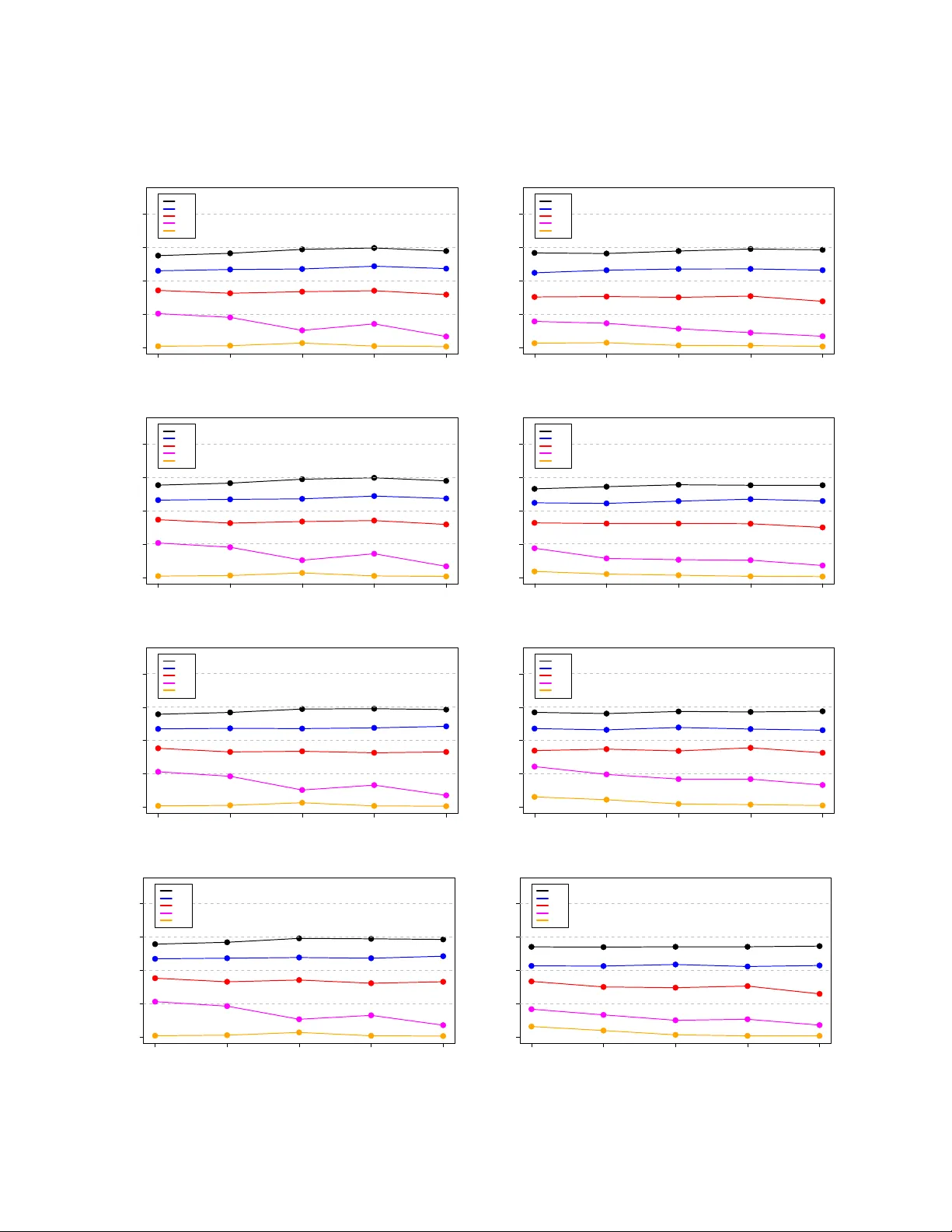
D aniel Suen university of w ashington Yen-Chi Chen university of w ashington F ebruary 20, 2026 Comp eting in terests: The authors declare none. Financial supp ort: DS w as supp orted b y NSF DGE-2140004. YC w as supp orted by NSF DMS-195278, NSF DMS-2112907, NSF DMS-2141808, and NIH U24-A G072122. Corresp ondence should b e sen t to E-Mail: dsuen@uw.edu Phone: 1-206-486-0446 Psychometrika Submission F ebruary 20, 2026 2 MODELING MUL TIV ARIA TE MISSINGNESS WITH TREE GRAPHS AND CONJUGA TE ODDS Abstract In this pap er, w e analyze a sp eciﬁc class of missing not at random (MNAR) assumptions called tr e e gr aphs , extending up on the work of pattern graphs. W e build oﬀ previous w ork b y introducing the idea of a conjugate o dds family in whic h certain parametric mo dels on the selection o dds can preserv e the data distribution family across all missing data patterns. Under a conjugate o dds family and a tree graph assumption, w e are able to mo del the full data distribution elegan tly in the sense that for the observ ed data, we obtain a mo del that is conjugate from the complete-data, and for the missing en tries, w e create a simple imputation mo del. In addition, we inv estigate the problem of graph selection, sensitivit y analysis, and statistical inference. Using b oth simulations and real data, w e illustrate the applicabilit y of our metho d. Key w ords: Missing data, Conjugate o dds, T ree graphs, Multiv ariate mo deling Psychometrika Submission F ebruary 20, 2026 3 1. In tro duction Missing data are p erv asiv e across healthcare, so cial sciences, economics, and mac hine learning. They arise from survey nonresp onse, equipment failure, priv acy concerns, and other sources, and the manner in whic h data are missing strongly inﬂuences the v alidit y of statistical analyses. When ignored, missingness can bias results and reduce statistical p o wer, esp ecially in large-scale studies where incomplete records are common ( R. J. A. Little & Rubin , 2002 ). Rubin’s framew ork classiﬁes missingness in to three categories ( R. J. Little & Rubin , 1989 ): missing completely at random (MCAR), missing at random (MAR), and missing not at random (MNAR). Standard approac hes are eﬀectiv e under MCAR or MAR, but MNAR p oses a fundamen tally harder problem: the probability of missingness dep ends on unobserv ed v alues, rendering the distribution uniden tiﬁable without further assumptions. The c hallenge is particularly acute in m ultiv ariate and nonmonotone settings, where missingness o ccurs irregularly across v ariables. Most practical metho ds rely on imputation, suc h as m ultiple imputation by chained equations ( mic e ; v an Buuren & Gro oth uis-Oudsho orn 2011 ) or MissF orest ( Stekho ven & B ¨ uhlmann , 2011 ), whic h are v alued for their ﬂexibilit y but implicitly assume MAR or rely on p oten tially incompatible conditionals. Moreo ver, metho ds such as MissF orest are also single imputation metho ds, whic h can lead to inconsisten t estimators, dep ending on the parameter of in terest. These limitations make them vulnerable to bias or incoherence under MNAR. Direct mo deling of imputation distributions is also diﬃcult because of high dimensionalit y and in terdep endence among v ariables, motiv ating the search for metho ds that are b oth in terpretable and theoretically principled. Tw o classical approac hes to MNAR are selection mo dels ( Diggle & Kenw ard , 1994 ) and pattern-mixture mo dels ( R. J. Little , 1993 ), whic h resp ectiv ely sp ecify missingness probabilities or stratify b y missingness patterns. While widely used, b oth require Psychometrika Submission F ebruary 20, 2026 4 un testable assumptions for identiﬁabilit y . More recen t strategies include “no self-censoring” assumptions ( Shpitser , 2016 ; Sadinle & Reiter , 2017 ), auxiliary v ariables ( Miao & Tc hetgen Tchetgen , 2016 ), and CCMV-t yp e restrictions ( Tchetgen Tchetgen et al. , 2018 ). Graphical frameworks, suc h as missing data DA Gs ( Mohan et al. , 2013 ) and pattern graphs ( Chen , 2022 ), pro vide p o werful representations of missingness assumptions, though their generalit y can mak e mo del selection challenging. This pap er builds on these adv ances by fo cusing on a structured and tractable sub class of pattern graphs, whic h w e term tree graphs. T ree graphs simplify mo del sp eciﬁcation, connect naturally to existing MNAR assumptions, and form the basis for scalable imputation strategies. T o complement this structure, we introduce the conjugate o dds prop ert y , which provides a ﬂexible parametric to ol for mo deling conditional distributions. T ogether, tree graphs and conjugate o dds yield a uniﬁed framew ork that ensures nonparametric iden tiﬁcation, facilitates inference, and enables practical sensitivity analysis. Outline. W e study tree graphs, a sp ecial case of pattern graph wtih nice prop erties in Section 2 and deriv e related theories. In Section 3 , we introduce the idea of conjugate o dds that is useful in domain adaptation. W e study how the conjugate o dds can b e used in handling missing data with tree graphs in Section 4 , whic h leads to an imputation mo del and a mo del on the observ ed data sim ultaneously . W e introduce three approaches for selecting a tree graph in Section 5 : prior knowledge, partial-ordering, and data-driven approac hes. In Section 6 , we apply the tree graph and conjugate o dds to an Alzheimer’s disease data. In app endices, we also inv estigate tree graph p erformance via simulation studies (App endix B ), and study the problem of statistical inferences (Appendix E ) and sensitivit y analysis (App endix F ). 1.1. Notation W e use a capital b oldface v ariable to denote a v ector-v alued random v ariable. In this pap er, w e consider a general problem setup, where X = ( X 1 , X 2 , . . . , X d ) ∈ R d is a random Psychometrika Submission F ebruary 20, 2026 5 v ector of v ariables. Eac h of the d v ariables can p ossibly b e missing for a total of up to 2 d missing patterns. Let R ∈ R ⊆ { 0 , 1 } d b e the random binary v ector that describ es the missing pattern asso ciated with X . W e write R j = 0 if and only if v ariable X j is missing. F or a ﬁxed pattern r , let X r = ( X j : r j = 1) denote the observ ed random v ariables and X ¯ r = ( X j : r j = 0) denote the missing random v ariables. When we write “F or j in r ,” this refers to the indices that con tain 1. F or example, supp ose X = ( X 1 , X 2 , X 3 , X 4 ) and r = 1001. W e hav e X r = ( X 1 , X 4 ) and X ¯ r = ( X 2 , X 3 ). Then, the statement “F or j in r ,” corresp onds to “F or j in 1, 4.” W e assume that the complete data is generated by sampling i.i.d. from the joint distribution p ( x, r ), and the resulting asso ciated pattern r generates the observ ed data. In this pap er, w e will use the terminology ful l-data distribution and p attern-sp e ciﬁc joint distribution to refer to p ( x, r ) and p ( x | r ), resp ectively . 2. T ree graphs and iden tiﬁcation theory 2.1. Pattern gr aphs Chen ( 2022 ) originally prop osed pattern graphs as a w a y to mo del nonmonotone missingness and nonparametrically iden tify the full-data distribution p ( x, r ). A pattern graph is a directed graph of missing data patterns that encodes a missing data assumption capable of nonparametrically iden tifying the full data distribution. In the pap er, he prop osed selection o dds and pattern-mixture mo del form ulations with resp ect to a giv en graph and sho w ed that the tw o are equiv alent. Estimation pro cedures using in verse probabilit y weigh ting, regression adjustment, and semiparametric eﬃciency theory w ere explored. Building on this work, we fo cus on a strict subset of pattern graphs called tr e e gr aphs . In this subsection, w e ﬁrst broadly summarize the previous w ork by introducing the notion of a pattern graph. W e imp ose a partial order on the patterns in R , where for an y distinct s, r ∈ R , we say s > r if and only if the observed v ariables in pattern r are also Psychometrika Submission F ebruary 20, 2026 6 observ ed in pattern s . F rom this partial order, we can construct a directed graph of all patterns, whic h forms the aforemen tioned p attern gr aph . Deﬁnition 1. A regular pattern graph is a directed graph of all patterns in R suc h that 1. Single source no de. P attern 1 d := (1 , 1 , 1 , 1 , . . . , 1 | {z } d times ) is the only source. 2. Regularit y . If there is an arrow present in the graph T from pattern s to pattern r , then s > r . The second prop erty refers to the regularit y and ensures that the graph is directed in a w ay that preserves the partial ordering of the patterns. P attern graphs represent information ﬂo w, whic h translates to a sp eciﬁc missing data assumption. Since we hav e a partial ordering of the missing patterns, w e assume that a pattern b orro ws information from its paren ts to mo del its missing data. Denote P A T ( r ) as the set of paren ts for pattern r in graph T . F ormally , the pattern-mixture mo del of ( X , R ) factorizes with resp ect to T if, w e ha ve p ( x ¯ r | x r , R = r ) T = p ( x ¯ r | x r , R ∈ P A T ( r )) ∀ r ∈ R . (P1) Equation ( P1 ) represen ts the pattern mixture mo del factorization prop ert y , which states that the extrap olation distribution under pattern r can b e iden tiﬁed using information from its parents. Additionally , the selection o dds mo del of ( X , R ) factorizes with resp ect to the graph if P ( R = r | x ) P ( R ∈ P A T ( r ) | x ) T = P ( R = r | x r ) P ( R ∈ P A T ( r ) | x r ) ∀ r ∈ R . (P2) Equation ( P2 ) represen ts the selection o dds factorization prop ert y , which states that the conditional o dds of a pattern r against its parents only dep ends on the commonly observ ed v ariables. Chen ( 2022 ) shows that equations ( P1 ) and ( P2 ) are equiv alent under very mild p ositivit y condition, so w e can interc hangeably using these tw o deﬁnitions. The pattern-mixture mo del form ulation illuminates the kind of assumption imp osed b y pattern Psychometrika Submission F ebruary 20, 2026 7 graph T . In particular, T asso ciates eac h pattern r with a set P A T ( r ) comprising closely related patterns whose observ ed v ariables also include those of r . F urther w ork by Zamanian et al. ( 2023 ) studied the sensitivit y analysis within the pattern graph framew ork. P atterns graphs hav e also recently b een used by Dong et al. ( 2025 ) in the con text of estimating equations. W e note that pattern graphs are not the con ven tional graphical mo del b ecause the no des here are represen ted by missing data patterns rather than individual v ariables. In previous missing data literature that use missing data D A Gs or m-DA Gs, one augments the usual directed acyclic graph of v ariables with no des for missingness indicators and edges capturing dep endencies ( Mohan et al. , 2013 ; Tian , 2015 ; Mohan & P earl , 2021 ). Phung et al. ( 2025 ) recently used a pattern DA G along with an m-D A G to help with identiﬁcation of the full-data distribution. 2.2. Deﬁnition and algebr aic pr op erties While pattern graphs encompass an exceptionally broad class of missing data assumptions, there are some ob vious shortcomings due to the ﬂexibilit y of the graph. A complex graph, while it is mathematically v alid, is not practically useful due to the fact that it w ould require one mo del on one edge within the graph. T o resolve this complexity issue while main taining the v alidit y of a graph, we now fo cus on a particular sub class of pattern graphs kno wn as tree graphs. T ree graphs represen t a ric h subset of pattern graphs, exhibiting notable algebraic and statistical prop erties that facilitate simpler estimation pro cedures and graph construction. The term tr e e gr aph is used to reﬂect its graphical structure, whic h resem bles a tree with a single ro ot no de. Moreo ver, several established missing data assumptions from the literature can b e incorp orated in to the pattern graph framew ork and reform ulated as tree graphs. Deﬁnition 2. (T ree graph) A tree graph is a regular pattern graph in whic h every pattern r  = 1 d has exactly one directed path originating from 1 d . Psychometrika Submission F ebruary 20, 2026 8 Pr op osition 1. Ev ery tree graph corresp onds to a unique missing not at random (MNAR) assumption that nonparametrically iden tiﬁes the full data distribution. Additionally , the selection o dds P ( R = r ℓ | X ) /P ( R = 1 d | X ) admits the follo wing iden tiﬁcation formula P ( R = r ℓ | X ) P ( R = 1 d | X ) tree graph = ℓ Y i =1 P ( R = r i | X r i ) P ( R = r i − 1 | X r i ) , where 1 d =: r 0 → r 1 → r 2 → · · · → r ℓ is the unique path in the tree graph from the source 1 d to pattern r ℓ . In this pap er, w e denote the set of tree graphs formed from d v ariables as T d . F or brevit y , we omit the subscript d and simply write T when the context makes it clear that w e are considering d v ariables. F rom the deﬁnition, we can see that a tree graph is a directed graph of the patterns in whic h there is a unique single path from the source 1 d to a giv en pattern r . In classical graph theory , this structure is also known as an arb or esc enc e ( F ournier , 2013 ). Prop osition 1 highlights a key identiﬁcation result for tree graphs. That is, a tree graph is a MNAR assumption that automatically nonparametrically identiﬁes the full data distribution. MNAR assumptions are notably diﬃcult to formulate. Pr op osition 2. If the data is missing completely at random (MCAR), then a tree graph assumption will still reco v er the true data distribution p ( x ). Prop osition 2 further emphasizes the fact that a tree graph assumption can still b e applied when the data could b e MCAR. T o make the graphical formulation more concrete, w e include t wo sp eciﬁc examples of common missing data assumptions that can b e reframed as tree graphs. In Example 1 , we discuss the complete-case missing v alue (CCMV) assumption ( R. J. Little , 1993 ; Tc hetgen Tc hetgen et al. , 2018 ; T an , 2023 ). Example 1. (Complete-case missing v alue (CCMV)) Our ﬁrst example is the Psychometrika Submission F ebruary 20, 2026 9 complete-case missing v alue, whic h is equiv alent to p ( x ¯ r | x r , R = r ) CCMV = p ( x ¯ r | x r , R = 1 d ) for all r ∈ R ( R. J. Little , 1993 ; Tchetgen Tchetgen et al. , 2018 ). This can b e viewed as a relaxation of a complete case analysis to an assumption that does not place constraints on the observ ed data. In particular, the complete case distribution is only used to deﬁne the extrap olation distributions. In con trast, a complete case analysis mak es the assumption that p ( x | R = r ) CCA = p ( x | R = 1 d ) for an y r ∈ R , which is essentially the missing completely at random. The righ t-hand side of the equation is the complete-case distribution while the left-hand side is the distribution of the data under a giv en pattern R = r . Since the LHS decomp oses as p ( x | R = r ) = p ( x ¯ r | x r , R = r ) p ( x r , R = r ), a complete-case analysis implictly places an assumption on the observ ed data and th us, may not agree with the observed data. The CCMV assumption b ypasses this b y only placing assumptions on the distribution of the missing v ariables, conditional on the observ ed data, and can b e viewed as a ﬁrst step ab ov e a naiv e CCA. F or a visual example, w e visualize the CCMV assumption in Figure 1 for d = 3 v ariables. F rom a graphical p ersp ectiv e, the CCMV assumption represen ts the most natural tree graph, as it forms the shallo w est structure. More broadly , tree graphs can b e viewed as generalizations of the CCMV assumption, allo wing for more complex paths from 1 d to the remaining patterns. In Example 2 , we discuss another tree graph assumption, nearest-case missing v alue (NCMV) in the con text of monotone missingness. Example 2. (Nearest-case missing v alue under monotone missingness) In our second example, w e consider a setting of monotone missingness in which the missing patterns form Psychometrika Submission F ebruary 20, 2026 10 Figure 1. (a) The CCMV tree graph for d = 3 v ariables. (b) The NCMV tree graph for d = 3 v ariables. an ordered set. F or simplicity , we assume that the missingness arises from drop out such that if v ariable X j is missing, then v ariable X j ′ is also missing for an y j ′ > j . F or notational conv enience, we denote each pattern by a p ositiv e in teger that denotes the index of the ﬁrst 0 in the missing pattern suc h that D = { 0 , 1 , 2 , 3 , 4 , 5 , 6 , . . . , d } . Then, the set D has a one-to-one corresp ondence with R = { 1 d , 1 d − 1 0 , 1 d − 2 00 , . . . , 0 d } , where the subscript denotes the num b er of 1s and 0s. Letting D denote the random v ariable asso ciated with D , the NCMV assumption is equiv alen t to p ( x >t | x ≤ t , D = t ) = p ( x >t | x ≤ t , D = t + 1) , P ( D = t | x ) P ( D = t + 1 | x ) = P ( D = t | x t ) P ( D = t + 1 | x t ) for all t ∈ D . W e visualize the NCMV assumption in Figure 1 for d = 3 v ariables. F rom Examples 1 and 2 , w e see that previously prop osed assumptions from the literature can b e cast in the tree graph framew ork. Through Prop osition 3 , we now in tro duce equiv alent deﬁnitions for tree graphs. Pr op osition 3. (Equiv alence deﬁnitions for tree graphs) Let T b e a pattern graph. The follo wing statements are equiv alent: 1. Unique directed path from 1 d . The pattern graph T is a tree graph with d v ariables. 2. Single paren t. Ev ery pattern r  = 1 d in T has exactly one paren t. Psychometrika Submission F ebruary 20, 2026 11 3. Minimal. There are 2 d − 1 edges in T . That is, T ac hieves the low er b ound on the n umber of edges that a pattern graph m ust hav e. Sev eral key practical insigh ts arise from these prop erties. First, since these form ulations are equiv alent, the prop osition pro vides multiple p ossible equiv alent deﬁnitions of a tree graph. Moreov er, as each pattern has exactly one parent, this gives us a straigh tforward metho d to b oth en umerate the class of tree graphs and construct a sp eciﬁc tree graph. The construction pro cess is further discussed in Section 5 . Next, minimalit y is closely link ed to mo del complexity . Missing not at random assumptions can b e notably exp onen tially complex. As the existence of an edge requires ﬁtting an additional selection o dds mo del, minimalit y ensures that the mo del complexit y for the global mo del p ( x, r ) is minimized within the space of pattern graphs and selection mo dels. 2.3. Enumer ation The size of the pattern graph set is astronomical as a function of the num b er of v ariables d ( Chen , 2022 ), illustrating that pattern graphs represen ts a h uge class of MNAR assumptions. While tree graph is just a subset of pattern graphs, the num b er of tree graphs stills gro ws signiﬁcan tly with the dimension d , so it also includes many MNAR assumptions. This is formalized with a low er b ound, which is presented in the following prop osition. Pr op osition 4. (Enumeration of tree graphs) The n umber of tree graphs is sup er-exp onen tial in the n umber of v ariables d . In particular, log |T d | ≳ d · 2 d . The size of the tree graph class gro ws rapidly . The exact form of our low er b ound is pro vided in the pro of, but w e note that when d = 5, w e ha ve |T d | ≥ 2 18 , and when d = 6, w e hav e |T d | ≥ 2 66 . Observe that the size of the class is largely due to the fact that the n umber of missing patterns is 2 d , exp onen tial in the n umber of v ariables. Ho w ever, in Psychometrika Submission F ebruary 20, 2026 12 practice, man y of these patterns ma y not b e observed in a given real data set. F or example, when the missingness is monotone, the n um b er of missing data patterns is d . Through some careful algebra, one can sho w that this reduces to the 2 O ( d 2 ) , whic h is still substan tial. Th us, the tree graph set remains a rich class of missing not at random assumptions while ha ving signiﬁcan t simpliﬁcations in the resulting mo del complexity . In Section 5 , w e discuss strategies for selecting a reasonable tree graph. 3. Conjugate o dds families and domain adaptation In the previous section, w e established that tree graphs pro vide a graphical represen tation for an MNAR assumption that iden tiﬁes the full data distribution. An additional b eneﬁt of the tree graph is that it allo ws a simple mo deling framew ork to estimate the pattern-sp eciﬁc data distribution via the graph structure b y transferring the complete data distribution in to eac h observed data distribution along the branch within a tree. This is inspired by T ukey’s factorization ( T ukey , 1986 ), which we will discuss in more detail in Section 4 . First, we discuss the idea of learning a target distribution from a source distribution. A common problem in statistics and mac hine learning is learning a target distribution p ( x | A = a ′ ) giv en kno wledge of a related distribution p ( x | A = a ). This setting is studied under domain adaptation and transfer learning, where kno wledge from a source distribution is adapted to a target one under distributional shift. F rom a generative mo deling p ersp ectiv e, this is closely related to densit y ratio estimation ( Sugiyama et al. , 2012 ). In the missing data setting, we view the distribution of complete cases ( R = 1 d ) as the source domain and the distribution under another missingness pattern R = r as the target. Since rare patterns often hav e few observ ations, direct estimation of the target distribution can b e infeasible, making domain adaptation particularly w ell-suited. Psychometrika Submission F ebruary 20, 2026 13 3.1. Exp onential tilting A natural starting p oin t is exp onen tial tilting (or exp onential change of measure) ( Essc her , 1932 ). Giv en a baseline density p 0 ( x ), the tilted distribution with parameter λ tak es the form p 1 ( x ) ∝ p 0 ( x ) e λT ( x ) ⇐ ⇒ p 1 ( x ) = p 0 ( x ) e λT ( x ) E p 0 [ e λT ( X ) ] , where T ( x ) is a statistic that is often chosen to b e the suﬃcient statistic in exp onential family mo dels, and the denominator ensures normalization. A k ey prop ert y of exp onential tilting is that it preserves the exp onential family structure. If the base distribution b elongs to an exp onential family with natural parameter η 0 , then the tilted distribution corresp onds to a simple shift in the natural parameter, η λ = η 0 + λ . This prop ert y enables eﬃcien t statistical computations, as it allows rew eighting while maintaining suﬃcient statistics and conjugate relationships. In our framew ork, exp onential tilting pro vides a principled wa y to adapt the complete-case distribution to appro ximate distributions under other missingness patterns, linking ideas from domain adaptation with tractable exp onen tial family mo dels. 3.2. Gener alizations to a c onjugate o dds pr op erty In this section, w e discuss a general mo deling strategy in whic h a parametric mo del is p osited for the source domain and under nice conditions, a simple parametric mo del can also b e obtained for the target domain. A starting p oint is to ﬁrst consider the factorization p ( x | A = a ′ ) ∝ p ( x | A = a ) · P ( A = a ′ | x ) P ( A = a | x ) . (3.1) F rom this factorization, w e see that the source distribution can b e p erturb ed to wards the target distribution b y m ultiplying by an o dds factors. In some situations, the o dds and the target distributions ha v e nice forms, which leads to the following idea of a conjugate o dds. Psychometrika Submission F ebruary 20, 2026 14 Deﬁnition 3. (Conjugate o dds) Let A ∈ A b e a categorical random v ariable that is auxiliary to the primary data X . Supp ose that p ( x | A = a ) and p ( x | A = a ′ ) b elong to the same probabilit y mo del P . Then, we say the mo del formed by O ( P ) := { O a ′ ,a ( x ) := P ( A = a ′ | x ) /P ( A = a | x ) : ∀ a, a ′ ∈ A} is a c onjugate o dds for P . In the deﬁnition for conjugate o dds, w e use the term conjugacy to relate it to the Ba yesian literature and the idea of conjugate priors. In Bay esian analysis, conjugate priors oﬀer an algebraic con v enience in that it provides a closed-form expression for the p osterior giv en a sp eciﬁc lik eliho o d function, thereby bypassing the need for n umerical integration or computational metho ds. In this pap er, we say that a given o dds family is c onjugate to a giv en family if it satisﬁes Deﬁnition 3 . Moreov er, the notion of conjugacy extends to a mixture mo del, where eac h comp onen t b elongs to the same parametric family , as seen in Prop osition 5 . 0.0 0.3 0.6 0.9 −1.0 −0.5 0.0 0.5 1.0 x Density Original Distribution 0 2 4 6 −1.0 −0.5 0.0 0.5 1.0 x F actor Tilting F actor e 2x 0.0 0.3 0.6 0.9 −1.0 −0.5 0.0 0.5 1.0 x Density T arget Distribution Figure 2. The left and right panels depict the original and target distribution (after tilting) on the in terv al [0 , 1]. The middle panel is the exp onential tilting factor e 2 x , which corresp onds to the weigh t placed at eac h part of the original distribution. Psychometrika Submission F ebruary 20, 2026 15 Pr op osition 5. (Conjugate o dds holds under mixtures) Supp ose that O ( P ) is a conjugate o dds for probabilit y mo del P . Then, O ( P ) is a conjugate o dds for the probabilit y K -mixture mo del, where eac h comp onen t is an element of P , M K ( P ) := ( p = K X j =1 w j p j     p j ∈ P , K X j =1 w j = 1 , w j > 0 ∀ j ) . W e note that in general, a rejection sampling sc heme is also p ossible. One can p osit a distribution for p ( x | A = a ), and ﬁt an y o dds mo del for O a ′ ( x ). This can b e any binary classiﬁer, whic h extends this metho dology to a suite of mac hine learning to ols. Then, as long as the o dds factor O a ′ ,a ( x ) is b ounded, then w e can do a rejection sampling sc heme b y using p ( x | A = a ) as a prop osal distribution to shift tow ards our desired p ( x | A = a ′ ). A b ounded o dds factor is reasonable if the v ariables X b elong to a b ounded set. Although we no longer ha v e a closed-form expression for the target distribution, we are able to p erform sampling. This idea is further explored in Section 4 . 3.3. L o gistic o dds No w, we provide our ﬁrst example of a conjugate o dds family b y demonstrating that logistic regression is a conjugate o dds for the exp onen tial family . Pr op osition 6. (Exp onential family , vector-v alued random v ariable) Supp ose that p ( x | A = a ) b elongs to the exp onen tial family parameterized b y η ∈ H , p ( x | A = a ; η ) = h ( x ) g ( η ) exp( η ⊤ T ( x )) Then, the asso ciated o dds mo del O a ′ ( x ; γ ) := log P ( A = a ′ | x ) P ( A = a | x ) = γ 0 + γ ⊤ T ( x ) , γ 0 := log P ( A = a ′ ) P ( A = a ) + log g ( η ′ ) g ( η ) holds if and only if p ( x | A = a ′ ; η ′ ) = h ( x ) g ( η ′ ) exp(( η ′ ) ⊤ T ( x )) , where η ′ := η + γ ∈ H . Psychometrika Submission F ebruary 20, 2026 16 A natural corollary of Prop osition 6 is the follo wing result, whic h establishes a link b et ween a logistic regression mo del and an exp onen tial tilting factor. Cor ol lary 1. (Exp onential tilting and logistic regression) Imp osing a logistic regression mo del on the o dds P ( A = a ′ | x ) /P ( A = a | x ) is equiv alen t to tilting a distribution p ( x | A = a ) b y an exp onen tial factor. Prop osition 6 has n umerous applications, as the exp onen tial family encompasses a broad class of parametric distributions for b oth discrete and con tin uous random v ariables, including the normal, exp onen tial, binomial, P oisson, and negative binomial distributions. Since exp onen tial tilting via logistic regression corresp onds to a translation in the natural parameter space, the range of p ossible v alues for the natural parameter is of fundamen tal imp ortance. This prop osition further implies that when logistic regression is p erformed using the suﬃcien t statistics of an exp onen tial family , the ﬁtted co eﬃcients of these statistics directly determine the parameterization of the new distribution p ( x | A = a ′ ). One k ey elemen t of the prop osition is the ﬁnal condition η ′ := η + γ ∈ H . Although an y pair of iden tically parameterized exp onential family distributions p ermits a logistic regression represen tation of the o dds, not all logistic regression and exp onen tial family distribution pairs yield an exp onen tial family represen tation for the target distribution. Similarly , not all exp onen tial tiltings lead to an exp onential family and ma y not even result in a v alid distribution. This discrepancy arises when the translation shifts the natural parameter b ey ond its v alid domain. Generally , this issue is mitigated when the natural parameter b elongs to an un b ounded space. F or instance, in the case of the binomial distribution, the natural parameter η := log p/ (1 − p ) b elongs to R , and any translation sta ys within the set. The result of Prop osition 5 can b e applied to the exp onen tial family , as seen in Corollary 2 . There are a few illuminating examples that fall under these sp eciﬁc conditions suc h as the Gaussian mixture mo del and binomial pro duct mixture mo del ( Suen & Chen , Psychometrika Submission F ebruary 20, 2026 17 2023 ). Cor ol lary 2. (Mixture of exp onential family) Supp ose that p ( x | A = a ) = K X k =1 w k · h ( x ) g ( η k ) exp( η ⊤ k T ( x )) , log P ( A = a ′ | x ) P ( A = a | x ) = γ 0 + γ ⊤ T ( x ) . Then, w e ha ve p ( x | A = a ′ ) = K X k =1 e w k · h ( x ) g ( η k + γ ) exp(( η k + γ ) ⊤ T ( x )) , where e w k := w k · g ( η k ) g ( η k + γ )  K X k ′ =1 w k ′ · g ( η k ′ ) g ( η k ′ + γ ) . Example 3. (Gaussian mixture mo del with isotropic v ariance) Since there are not man y conv enient options for oﬀ-the-shelf mo deling of m ultiv ariate contin uous data, practitioners often use a Gaussian mixture mo del for its ﬂexibilit y and relativ ely easy asso ciated estimation pro cedure. Supp ose that p ( x | A = a ) = K X k =1 w k · d Y j =1 1 σ 2 k,j √ 2 π exp − 1 2 σ 2 k,j ( x j − µ k,j ) 2 ! , log P ( A = a ′ | x ) P ( A = a | x ) = γ 0 + γ ⊤ 1 x + γ ⊤ 2 x 2 . Then, p ( x | A = a ′ ) = K X k =1 w k · d Y j =1 1 σ ′ k,j 2 √ 2 π exp − 1 2 σ ′ k,j 2 ( x j − µ ′ k,j ) 2 ! , where µ ′ k,j := µ k,j /σ 2 k,j + γ 1 ,j 1 /σ 2 k,j − 2 γ 2 ,j , ( σ 2 k,j ) ′ := 1 1 /σ 2 k,j − 2 γ 2 ,j , and w ′ k = w k · g ( η k ) g ( η k + γ )  K X k =1 w k · g ( η k ) g ( η k + γ ) for g ( η 1 , η 2 ) = Q d j =1 g ( η j, 1 , η j, 2 ) = Q d j =1 exp  η 2 j, 1 4 η 2 j, 2  · p − 2 η j, 2 . Psychometrika Submission F ebruary 20, 2026 18 Example 4. (Binomial pro duct mixture mo del) Previously , Suen & Chen ( 2023 ) in tro duced the binomial pro duct mixture mo del to mo del m ultiv ariate discrete data. Supp ose that p ( x | A = a ; w , p ) = K X k =1 w k · d Y j =1  N j x j  p x j k,j (1 − p k,j ) N j − x j , log P ( A = a ′ | x ) P ( A = a | x ) = γ 0 + γ ⊤ x. Then, p ( x | A = a ′ ; w ′ , p ′ ) = K X k =1 w ′ k · d Y j =1  N j x j  p ′ k,j x j (1 − p ′ k,j x j ) N j − x j , where p ′ k,j = exp(logit( p k,j ) + γ j ) 1 + exp(logit( p k,j ) + γ j ) and w ′ k = w k · g ( η k ) g ( η k + γ )  K X k =1 w k · g ( η k ) g ( η k + γ ) for g ( ζ ) = Q d j =1 1 (1 + exp( − ζ j )) N j . Example 5. (Gaussian k ernel density estimator) Supp ose that p ( x | A = a ) is ﬁt nonparametrically using a k ernel densit y estimator with a pro duct Gaussian kernel as follo ws b p ( x | A = a ) = 1 nh d n X i =1 d Y j =1 K  x j − X i,j h  , where K ( t ) = 1 √ 2 π exp( − 1 2 t 2 ). Th us, the KDE is a Gaussian mixture mo del with n comp onen ts (equally weigh ted), eac h b eing a m ultiv ariate Gaussian centered at each data p oint with cov ariance matrix diag( h 2 , h 2 , . . . , h 2 ). Then, from Example 3 , it follows that b p ( x | A = a ′ ) is a w eigh ted Gaussian k ernel densit y estimator. The logistic mo del for o dds is not the only p ossible mo del for conjugate o dds; in App endix C , w e pro vide an example of p ow er law o dds. Psychometrika Submission F ebruary 20, 2026 19 4. T ree graphs and conjugate o dds With the conjugate o dds, w e dev elop an easy wa y to construct estimates of 1) the imputation distribution p ( x ¯ r | x r , R = r ) and 2) the conditional distribution p ( x | R = r ). W e demonstrate that b oth of these tasks can b e ac hiev ed in one shot by unifying the t wo framew orks (tree graph and conjugate o dds) through the idea of T uk ey’s factorization. A feature of tree graph is that our mo del on p ( x | R = r ) includes b oth observed v ariables as w ell as the missing v ariables. Therefore, the marginal distribution p ( x ) can b e obtain easily . Deﬁnition 4. (T uk ey’s factorization, ( T ukey , 1986 )) Consider a univ ariate Y ∈ R that is observ ed if R = 1 and not observ ed if R = 0. W e hav e the following factorization p ( y | R = r ) = p ( y | R = 1) · P ( R = r | y ) P ( R = 1 | y ) · P ( R = 1) P ( R = r ) . In tro duced by T ukey in a discussion ( T ukey , 1986 ), the adv antage of the ab o ve factorization is that iden tiﬁes the missing data distribution as a pro duct of t wo terms (one of whic h is p ( y | R = 1) and can b e estimated easily) and an o dds term, whic h can b e easier to think ab out and can naturally arise in man y applications. The key observ ation is that the ab o ve equation is reminiscen t of an aforementioned factorization for tilting a distribution (Equation ( 3.1 )). The term p ( y | R = 1) is directly iden tiﬁable from the observ ed data. The o dds term P ( R = r | y ) /P ( R = 1 | y ) dep ends on unobserved data, but can b e iden tiﬁed using the tree graph framew ork. F rom here, we can exp ect to b orrow the to ols from conjugate o dds framew ork to tilt the complete case distribution p ( x | 1 d ). F ranks et al. ( 2020 ) previously built on the idea of T ukey’s factorization as an alternativ e metho d from pattern-mixture mo dels and selections mo dels for mo deling the full-data distribution. In their work, they discuss this mo deling strategy with a a single v ariable and tw o p ossible missing patterns. W e extend this work to handle the multiv ariate case. T ukey’s original factorization can b e naturally generalized to a multiv ariate setting, as seen in the follo wing deﬁnition that w e prop ose. Psychometrika Submission F ebruary 20, 2026 20 Deﬁnition 5. (Multiv ariate T uk ey’s factorization) Consider a multiv ariate X ∈ X ⊆ R d with an asso ciated missing pattern R . W e hav e the following factorization p ( x | R = r ) = p ( x | R = 1 d ) · P ( R = r | x ) P ( R = 1 | x ) · P ( R = 1 d ) P ( R = r ) . As in the univ ariate case, the ab o v e factorization demonstrates that p ( x | R = r ) is prop ortional to a pro duct of t w o terms: the complete case distribution p ( x | R = 1 d ) and an o dds term P ( R = r | x ) /P ( R = 1 d | x ). That is, this is another factorization for tilting a distribution as in Equation ( 3.1 ). Imp ortantly , this selection o dds term is not directly iden tiﬁable without further assumptions. Ho wev er, Prop osition 1 shows that under a tree graph assumption, these selection o dds admits an elegan t iden tiﬁcation formula and can b e estimated using the observ ed data. Assumption 1. (Absolute con tinuit y with resp ect to the complete case distribution) The distribution p ( x | R = r ) is absolutely con tin uous with resp ect to the complete case distribution p ( x | R = 1 d ) for an y r  = 1 d . When utilizing T uk ey’s factorization, one implicitly is making an assumption. Assumption 1 arises from the nonnegativit y of the selection o dds nonnegativ e: if p ( x | R = 1 d ) = 0, then p ( x | r ) = 0 m ust hold. If the complete case distribution satisﬁes a p ositivit y condition where p ( x | R = 1 d ) > 0 for all x ∈ X , then this assumption will b e trivially satisﬁed. F or instance, the mixture mo dels presented in Section 3 satisfy this p ositivit y condition since eac h mixture comp onent has p ositive probability on all of X . W e no w harmonize the t wo frameworks with the following theorem. The or em 1. (Mo deling pattern-sp eciﬁc joint distributions using tree graphs and conjugate o dds) Supp ose the follo wing conditions hold: 1. The missingness mechanism is sp eciﬁed using a tree graph assumption. Psychometrika Submission F ebruary 20, 2026 21 2. The o dds mo del for the selection o dds is conjugate to the p ( x | R = 1 d ) mo del. Then, the pattern-sp eciﬁc joint distributions p ( x | R = r ) for all r b elong to the same family as p ( x | R = 1 d ). Theorem 1 is v ery p o werful b ecause it combines a tree graph and the conjugate o dds prop ert y in the missing data con text and demonstrates how that can lead to elegant mo deling of the pattern-sp eciﬁc join t distributions p ( x | R = r ). Example 6. (T ree graph with logistic regression and Gaussian mo del) Supp ose that a tree graph assumption holds, and the selection o dds can all be mo deled using a logistic regression. Then, if p ( x | R = 1 d ) b elongs to an exp onen tial family , then p ( x | R = r ) for any r ∈ R is also exp onential family . In particular, supp ose that • p ( x | R = 1 d ) is a m ultiv ariate Gaussian • all the selection o dds can b e mo deled using logistic regression (log[ P ( R = r | x ) /P ( R ∈ P A T ( r ) | x )] = γ 0 ,r + γ ⊤ r T ( x r ) with T ( · ) b eing a linear function) then all the pattern-sp eciﬁc join t distributions p ( x | R = r ) for all r are multiv ariate Gaussian. This idea generalizes to exp onential family mo dels and mixtures of exp onential family mo dels due to Prop ositions 5 and 6 . A further consequence of Deﬁnition 5 is that imp osing a tree graph assumption and mo dels for the o dds leads to an explicit closed-form expression form p ( x | R = r ). Notably , this distribution factorizes as p ( x ¯ r | x r , r ) p ( x r | r ), so the aforemen tioned pro cedure mo dels b oth the observ ed data distribution and the missing data distribution in one shot. This is an adv an tage ov er other metho ds such as mic e , which are able to generate Monte Carlo estimates from the imputation distribution but do not sp ecify a form for the density of the Psychometrika Submission F ebruary 20, 2026 22 observ ed or missing data distributions. Because we obtain a sp eciﬁc form for the pattern-sp eciﬁc join t distribution p ( x | R = r ) due to conjugacy , it is easier to interpret and also p erform imputation without ha ving to reﬁt an ything. 4.1. Imputation via a c onjugate o dds appr o ach In some settings, estimating a join t mo del p ( x, r ) is not the end goal. F or example, some migh t w ant to complete the data using an imputation. As previously mentioned, we are able to obtain a closed-form expression for the imputation distribution due to conjugacy . W e outline this in Algorithm 1 . Algorithm 1 Conjugate o dds imputation under logistic regression and exp onen tial family Require: { ( X i, R i , R i ) } n i =1 , a tree graph T 1: Fit the complete case mo del p ( x | 1 d ; θ ) with natural parameter η . 2: for r  = 1 d do 3: Fit the logistic regression mo del O r ( x r ; β r ) := P ( R = r | x r ) /P ( R ∈ P A T ( r ) | x r ) under the tree graph T 4: for r  = 1 d do 5: Compute the selection o dds with resp ect to the source 1 d via O r :1 d ( x ; λ r ) := Q r ′ O r ′ ( x r ′ ; β r ′ ). 6: F orm the parameter of the distribution p ( x | R = r ; θ r ) via θ r := η − 1 ( η + λ r ). 7: for m = 1 , 2 , . . . , M do 8: for i = 1 , 2 , . . . , n do 9: if R i  = 1 d then 10: Impute e X ( m ) i, ¯ R i using the distribution p ( x ¯ r | x r , R = r ). 11: Set the m -th imputed data to b e e X ( m ) i := ( X i, R i , e X ( m ) i, ¯ R i ). 12: return n e X ( m ) i o i =1 ,...,n m =1 ,...,M Psychometrika Submission F ebruary 20, 2026 23 4.2. R eje ction sampling for imputation When o dds are not mo deling using a conjugate o dds, then there ma y b e c hallenges in ﬁnding a closed form expression for the imputation distribution. How ever, provided that the o dds terms are b ounded a w ay from inﬁnity , it is p ossible to p erform rejection sampling. The k ey requiremen t is that there exists a constant U r suc h that the target densit y f ( x ) satisﬁes f ( x ) ≤ U r · g ( x ) for all x , where g ( x ) is the prop osal density . Here w e would simply tak e the prop osal distribution to b e the complete case distribution p ( x ¯ r | x r , R = 1 d ) and the target distribution to b e p ( x ¯ r | x r , R = r ), our true imputation distribution. Since the o dds terms are b ounded, this ensures that suc h an U r exists, making the rejection sampling pro cedure feasible. W e outline this metho d in Algorithm 2 . Although this approac h ma y in tro duce additional computational o verhead, it oﬀers a ﬂexible alternative when traditional sampling metho ds are not applicable due to the lac k of a closed-form expression. 5. Strategies for tree graph selection As established in Section 2.3 , the n um b er of tree graphs grows sup er-exp onentially with the n um b er of v ariables, making graph selection challenging. Moreo ver, Prop osition 1 sho ws that eac h tree graph enco des an MNAR assumption that cannot b e rejected from observ ed data, underscoring the c hallenge for systematic selection strategies. F rom the single-paren t prop ert y of Prop osition 3 , selecting a tree graph is equiv alent to assigning each pattern a unique paren t. This deﬁnes a function P A G : R\{ 1 d } → R with P A G ( r ) > r for all r ∈ R , oﬀering a compact and eﬃcient wa y to enco de tree structures. T o guide practical construction, w e prop ose three principles: 1. Prior kno wledge. Select a parent for each pattern that follows prior or scientiﬁc kno wledge. 2. Partial ordering. Select a parent for each pattern based on an existing partial ordering principle (suc h as CCMV or NCMV). W e discuss generalizations of the NCMV Psychometrika Submission F ebruary 20, 2026 24 Algorithm 2 Imputation via rejection sampling under logistic regression and exp onential family Require: { ( X i, R i , R i ) } n i =1 , U r (an upp er b ound on the o dds for pattern r ), a tree graph T 1: Fit the complete case mo del p ( x | 1 d ; θ ) with natural parameter η . 2: for r  = 1 d do 3: Fit the logistic regression mo del O r ( x r ; β r ) := P ( R = r | x r ) /P ( R ∈ P A T ( r ) | x r ) under the tree graph T 4: for r  = 1 d do 5: Compute the selection o dds with resp ect to the source 1 d via O r :1 d ( x ; λ r ) := Q r ′ O r ′ ( x r ′ ; β r ′ ). 6: F orm the parameter of the distribution p ( x | R = r ; θ r ) via θ r := η − 1 ( η + λ r ). 7: for m = 1 , 2 , . . . , M do 8: for i = 1 , 2 , . . . , n do 9: if R i  = 1 d then 10: while Y ( m ) is not accepted do 11: Sample a prop osal Y ( m ) ∼ p ( x ¯ r | x r , R = 1 d ). 12: Accept Y ( m ) with probabilit y p ( Y ( m ) | x r , R = r ) U r · p ( Y ( m ) | x r , R =1 d ) . 13: Set the m -th imputed data to b e e X ( m ) i := ( X i, R i , Y ( m ) ). 14: return n e X ( m ) i o i =1 ,...,n m =1 ,...,M Psychometrika Submission F ebruary 20, 2026 25 assumption to nonmonotone data in a later subsection. 3. Observed data distribution alignmen t. If the observed data distributions under t wo missing patterns are similar, w e may exp ect that the missing data distributions corresp onding to the same missing patterns are similar as w ell. Here we can use the data to iden tify most relev an t parents to a given child. W e pro vide tw o metho ds based on distributional distance. In addition to the ab o v e three principles, one may randomly choose a tree graph and p erform inference. W e provide a simple algorithm on how to sample a tree graph in App endix D . 5.1. Prior know le dge The ﬁrst and most fundamen tal principle is to lev erage prior knowledge when selecting a paren t for eac h pattern. Scien tiﬁc insigh ts, domain exp ertise, or w ell-established theoretical foundations can pro vide strong guidance in determining plausible paren t-child relationships. F or instance, in a biological setting, hierarchical dep endencies b etw een genetic mark ers ma y b e informed by known pathw ays or functional interactions. Similarly , in causal inference, domain kno wledge ma y suggest directional dep endencies b etw een observ ed v ariables. By incorp orating prior knowledge into the selection pro cess, we ensure that the tree graph aligns with meaningful, in terpretable structures that reﬂect real-w orld mec hanisms. Example 7. (Longitudinal study with missingness due to drop out) Consider a longitudinal study where the same test is measured with at regualar time interv als. Then, supp ose there is monotone missingness due to drop out. W e might hypothesize that individuals with missing pattern R = 1000 and R = 0000 are closely related b ecause we migh t reason that individuals that nev er show ed up to the study are most similar to Psychometrika Submission F ebruary 20, 2026 26 individuals who only sho w ed up to the ﬁrst time p oin t. Then, one can connect the patterns 1000 → 0000. This is related to the nearest-case missing v alue assumption (NCMV; Thijs et al. ( 2002 )). Example 8. (Hierarc hical data collection pro cesses) Supp ose we hav e four collected v ariables: X 1 , which corresp onds to a routine c heck-up measure suc h as blo o d pressure, X 2 , represen ting a disease state lik e chronic kidney disease (CKD), X 3 , whic h measures sw elling (a common symptom of CKD), and X 4 , a clinical test result assessing kidney function. In medical settings, it is common for X 3 and X 4 to b e recorded only when X 2 exceeds a certain threshold, indicating a more sev ere condition. Consequently , missing data patterns suc h as R = 1000, 0100, and 1100 ma y arise. Since individuals missing X 3 and X 4 are lik ely healthier, it is plausible to infer hierarc hical relationships b etw een these missing patterns, suc h as 1100 → 1000 and 1100 → 0100, where the presence of b oth symptom and test data informs cases where only one or neither is recorded. Example 9. (Group similarit y) Supp ose we hav e three v ariables: X 1 , a self-rep orted stress lev el, X 2 , alcohol consumption (e.g., self-rep orted drinks p er w eek), and X 3 exercise habits (e.g., frequency of ph ysical activit y p er week). There ma y b e a so cial stigma asso ciated with alcohol, whic h is related to underrep orting and ev en missingness. W e p osit that the groups R = 100 and 101 are similar in that they are more likely to suﬀer from suc h so cial stigma, so w e may suggest a relationship 101 → 100. 5.2. Partial or dering In monotone missing data problem, some assumptions, suc h as nearest case missing v alue (NCMV), utilizes an ordering on missing data patterns and also admit scien tiﬁc in terpretations. This is p ossible b ecause in the monotone missing data setting, and each pattern has a paren t that is the unique pattern that con tains exactly one more observ ed v ariable. In the nonmonotone missing data setting, the p ossible parent is no longer unique Psychometrika Submission F ebruary 20, 2026 27 Figure 3. The left panel corresp onds to the tree graph for d = 3 v ariables and the leftmost-ﬁrst NCMV (LNCMV) assumption. The righ t panel corresp onds to the tree graph for d = 3 v ariables and the rightmost-ﬁrst NCMV (RNCMV) assumption. b ecause there are m ultiple p ossible patterns that con tain one more observed v ariable. F or example, in the monotone missing data situation 1000 w ould ha ve parent 1100, but in the nonmonotone missing data setting, it could ha ve parent 1100, 1010, or 1001. T o resolve this issue, w e relax the ordering in to partial ordering and prop ose the following generalization. Deﬁnition 6. (Generalized nearest case missing v alue (GNCMV)) A tree graph is called a gener alize d ne ar est c ase missing value assumption if ev ery pattern in the graph has a paren t that con tains exactly one more observed v ariable. The GNCMV is still a large class of tree graphs. T o choose a reasonable tree under GNCMV, w e consider t wo sp ecial cases: the leftmost ﬁrst appr o ach (LNCMV) and the rightmost ﬁrst appr o ach (RNCMV). LNCMV is the tree graph where the parent is the pattern where the leftmost ﬁrst 0 (missing v araible) is replaced b y 1. RNCMV is deﬁned similarly but w e replace the righ tmost ﬁrst 0 by 1. F or example, the pattern 01010 has three p ossible paren ts under GNCMV: 11010, 01110, 01011. The LNCMV c ho oses 11010 as its paren t while RNCMV c ho oses 01011. W e visualize b oth of these ideas in Figure 3 . Pr op osition 7. (Generalized nearest-case missing v alue tree graphs) Denote the subset Psychometrika Submission F ebruary 20, 2026 28 of tree graphs that exhibit the GNCMV prop ert y as T GNCMV . W e hav e log |T GNCMV | ≳ 2 d . Moreo ver, for any T ∈ T GNCMV , T exhibits the following prop erties: 1. It achiev es the maximum p ossible depth of d . 2. Every pattern r in T is p ositioned at the maxim um p ossible distance from the source no de 1 d , thereb y corresp onding to the most information ﬂo w. Observ e that b y pruning the nonmonotone patterns from each graph, we recov er the tree structure that w ould exist under the NCMV assumption with monotone missingness. Moreo ver, the k -th lay er contains  n k  patterns. This assumption stands in direct contrast to the CCMV assumption, as eac h pattern is p ositioned at the maxim um p ossible distance from the source, represen ting the opp osite structural arrangemen t. 5.3. Observe d data distribution alignment When attempting to infer the structure of a tree graph from data, a natural question is: how should we identify the most plausible parent no des for a given no de? Our data-driv en metho d oﬀers a principled w ay to rank candidate parents using observed distributions. The data-driven metho d is an approach one can use to rank p otential paren ts from the data, thereb y informing the tree graph structure from the existing data. By assumption, the tree graph asserts the follo wing equalit y for every pattern r p ( x ¯ r | x r , R = r ) T = p ( x ¯ r | x r , R = P A T ( r )) . Th us, one natural idea is to only matc h extrap olation distributions if the observed data distributions under b oth R = r and R ∈ P A T ( r ) are similar. More precisely , we would desire d ( p ( x r | R = r ) , p ( x r | R = P A T ( r ))) to b e small for some probabilit y metric or div ergence d . This motiv ates t wo p ossible matching approac hes. While w e describ e them in the context of a lik eliho o d method, we note that matc hing approaches can b e more general. Psychometrika Submission F ebruary 20, 2026 29 P aren t-based alignmen t. In the ﬁrst, supp ose we obtain data X 1 ,r , X 2 ,r , . . . , X n r ,r ∼ p ( x r | r ) and attempt to determine whic h paren t distribution p ( x r | s ) has the b est ﬁt, among all p ossible paren ts s . In practice, for each s ∈ PP A( r ), we ﬁt a parametric mo del for p ( x r | s ) and estimate the exp ected log-lik eliho o d calculated on the data. This pro cedure can b e expressed in the p opulation version as argmax s ∈ PP A( r ) E X r ∼ p ( x r | R = r ) [log p ( X r | R = s )] . The KL div ergence pro vides an alternate p ersp ective. Through a series of equalities, w e hav e argmin s ∈ PP A( r ) D KL ( p ( x r | R = r ) || p ( x r | R = s )) = argmin s ∈ PP A( r ) Z ∞ −∞ p ( x r | r ) log p ( x r | r ) p ( x r | s ) dx r = argmax s ∈ PP A( r ) Z ∞ −∞ p ( x r | r ) log p ( x r | s ) dx r = argmax s ∈ PP A( r ) E [ ℓ ( X r | s )] . This highligh ts the fact that the maximization pro cedure w e prop ose is directly equiv alent to pic king the pattern that minimizes the sample v ersion of the KL divergence b etw een p ( x r | R = r ) and p ( x r | R = s ). Implementation of this pro cedure in practice can b e most eﬃcien tly done b y ﬁrst estimating each mo del p ( x r | r ) for all r ∈ R and then storing each mo del. W e present connections to the KL divergence, but we also note that one could certainly extend this to other distances. More generally , other f -divergences or metrics suc h as the W asserstein distance could b e explored, particularly when distributional smo othness or supp ort mismatch is a concern. F or example, the Hellinger distance can also b e utilized and has the nice prop erty that it is a b ounded metric. While the KL divergence is easy to implemen t with a giv en mo del, it is generally not p ossible in nonparametric settings. In those settings, one could consider distances b etw een distributions via an energy-based approac h. W e provide an example of ho w this could b e done in App endix A.2 . Child-based alignmen t. There is an alternative approach through a child-based alignmen t approach. In con trast to the ab o ve, supp ose we obtain data Psychometrika Submission F ebruary 20, 2026 30 X 1 ,s , X 2 ,s , . . . , X n s ,s ∼ p ( x s | s ) and attempt to determine whic h c hild distribution p ( x r | r ) has the b est ﬁt. W e outline this in further detail in the App endix. Pro vided the ﬁtted mo dels are stored in memory , b oth the paren t-based and c hild-based approaches hav e similar computational complexit y , but the paren t-based metho d has an illuminating theoretical in terpretation when using the KL div ergence. Note that if a prop er distance/metric is used to compare distributions, the paren t-based and c hild-based alignmen t b e the same; their diﬀerence is due to the asymmetry of the KL div ergence. In sim ulation, we demonstrate that b oth the paren t-based and child-based mo deling approac hes are able to learn the correct tree graph giv en enough sample size in some settings. This is discussed in App endix B . 6. Real data Here w e illustrate the applicabilit y of our metho d using an Alzheimer’s disease data with a mixture of binomial pro duct mo del. W e also provide an example of using KDE on wine data in App endix A . 6.1. NA CC data W e consider the analysis of neuropsyc hological test scores in the database of the National Alzheimer’s Co ordinating Cen ter (NA CC) 1 . The National Alzheimer’s Co ordinating Cen ter (NA CC), funded by the NIH and NIA, ov ersees the largest longitudinal database on Alzheimer’s disease in the United States. It serves as a co ordinating hub for 33 Alzheimer’s Disease Researc h Cen ters (ADRCs) across the country . This data set comprises individuals of v arying cognitiv e status: cognitively normal to mild cognitiv e impairment (MCI) to demen tia. Eac h individual is assigned a CDR (clinical demen tia rating) from clinician with 0 corresp onding to cognitiv ely normal, 0.5 1 h ttps://naccdata.org/ Psychometrika Submission F ebruary 20, 2026 31 corresp onding to mild cognitiv e impairmen t, and 1, 2, and 3 corresp onding to mild, mo derate, and sev ere demen tia, resp ectively . T ypically , neuropsychological assessments are conducted annually , but incomplete outcome data is common for v arious reasons. In some cases, sp eciﬁc tests are discontin ued o ver time and substituted with alternativ e measures. In others, missing scores may result from do cumen tation errors or from participan ts b eing to o unw ell to complete further testing. 6.1.1. Description of outc ome variables and c ovariates Our main goal is to measure and mo del the cognitiv e abilit y of the Alzheimer’s disease patien ts. W e fo cus on the following v ariable UDSBENTD, which is the total score for ten to ﬁfteen min ute dela yed drawing of Benson ﬁgure. In the Benson ﬁgure test, a participant is presen ted with a diagram of a complex ﬁgure and is ask ed to cop y it. After a perio d of ab out ten to ﬁfteen min utes, they are ask ed to recopy it again from memory , and they are assigned a score from 0 to 17 based on ho w w ell it resembles the original ﬁgure. This test measures visuospatial, visual memory , and executiv e abilities. W e lo ok at individuals who en tered the study from the y ears 2015 to 2019 and follow them for ﬁve years total, examining the rep eated dela y ed Benson ﬁgure test score each year. W e do not use the CDR score in the mo del, but w e use to help rep ort and in terpret the results. W e ﬁrst plot the missing pattern distribution in Figure 4 . W e can initially observe that the complete cases are v ery small with n cc = 271 individuals out of a p ossible n = 13440. Additionally , ev ery p ossible pattern of the 16 p ossible is observed, ranging from R = 10000 to R = 11111. The distribution is primarily dominated by the monotone missing patterns 10000, 11000, 11100, 11110, and 11111, lik ely due to drop out. Of primary in terest, we will examine the patterns 10000, 11000, 10100, and 10010 b ecause they are some of the larger patterns. Psychometrika Submission F ebruary 20, 2026 32 Missing Pattern Distrib ution for UDSBENTD (n = 13440) Binary Representation Count 0 1000 2000 3000 4000 5000 10000 10001 10010 10011 10100 10101 10110 10111 11000 11001 11010 11011 11100 11101 11110 11111 Figure 4. This is the missing pattern distribution for the UDSBENTD v ariable ov er 5 years. 6.1.2. A nalysis of NACC data W e next plot four diﬀeren t tree graphs of in terest: LNCMV, RNCMV, parent-based mo deling, and c hild-based mo deling. These four tree graphs are rep orted in Figure 5 . In terestingly , they all share similar maxim um depth. The parent-based mo deling is able to generally able to reco v er the LNCMV principle for many of the patterns, including most of the monotone missing patterns. On the other hand, the child-based mo deling app ears to incorp orate a mix of b oth LNCMV and RNCMV principles when assigning a pattern to a giv en parent. Because the patterns 10000, 11000, 10100, and 10010 each share similar ancestors in b oth the LNCMV and paren t-based mo deling tree graph, w e would exp ect that the t w o tree graphs lead to similar ﬁtted distributions at the end. In Figure 6 , w e plot the results of the ﬁtted mo del p ( x | R = 1 d ) using a mixture of binomial pro ducts. W e ﬁt it using 5 clusters b ecause of the recommendation from BIC. F rom the ﬁrst ﬁv e panels, w e can see that it is roughly able to capture the shap e of the Psychometrika Submission F ebruary 20, 2026 33 LNCMV − UDSBENTD 11000 11001 11010 11011 11100 11101 11110 11111 10000 10001 10010 10011 10100 10101 10110 10111 RNCMV − UDSBENTD 10001 10011 10111 10101 11111 11001 11011 11101 10000 10010 10100 10110 11000 11010 11100 11110 P arent−Based Modeling − UDSBENTD 11000 11011 11110 11111 11100 11101 10000 10001 10010 10011 10100 10101 10110 10111 11001 11010 Child−Based Modeling − UDSBENTD 10011 11111 10101 11101 11001 11011 10000 10001 10010 10100 10110 10111 11000 11010 11100 11110 Figure 5. These are the tree graphs for the UDSBENTD data analysis obtained via diﬀeren t metho ds: LNCMV, RNCMV, parent-based mo deling, and child-based mo deling. Psychometrika Submission F ebruary 20, 2026 34 1 2 3 4 5 0 5 10 15 20 CC Clusters Y ear UDSBENTD Score 0.21 0.41 0.27 0.07 0.05 10.2 10.3 10.3 10.6 10.3 (n = 271) 0.04 0.06 0.04 0.06 0.03 0.15 0.12 0.11 0.12 0.16 0.27 0.32 0.3 0.31 0.36 0.56 0.67 0.69 0.78 0.97 0.61 0.75 0.79 0.86 1.18 Figure 6. Fitting the mixture of binomial products mo del on the complete case distribution with k = 5 comp onents. Eac h comp onen t’s parameters corresp ond to a curve. The num b ers on top of each parameter v alue indicates the av erage CDR score, a clinical measuremen t of the cognitive decline level, which was not used in our mo del ﬁtting (the CDR score serves as a external v alidation of our ﬁtted mo del). Note that for the pink comp onen t, it shows a learning eﬀect on y ear 3 to year 4 that the score was improving while the clinical assessmen t (CDR score) of the cognitiv e abilit y is declining. marginal distributions. In the sixth panel, we include plots of the ﬁve clusters we obtain as laten t tra jectories o ver the ﬁv e time p oints. Eac h cluster is represented by a curv e with the observ ed a verage CDR score rep orted at eac h dot. A given dot corresp onds to the predicted mean UDSBENTD score from the mo del for a giv en cluster and y ear. Because the av erage CDR score is close to 0, the ﬁrst t w o clusters represent cognitively normal p eople. There is also some evidence of a practice eﬀect b et w een years 1 and 3 b ecause the scores increase o ver those years ( Goldb erg et al. , 2015 ). The third clusters can b e interpreted as mild cognitiv ely impaired p eople b ecause the a verage CDR score is close to 0.5. The fourth cluster app ears to represen t mild cognitiv ely impaired p eople transitioning to dementia. The ﬁfth cluster app ears to b e mostly mildly cognitiv e impaired or demen tia individuals. In Figure 7 , w e plot our ﬁtted mo del using the conjugate o dds metho d against the Psychometrika Submission F ebruary 20, 2026 35 0 5 10 15 0.00 0.05 0.10 0.15 0.20 0.25 Empirical p(x1|R=10000) with MixtureBinomProd Overlay x Probability CCA RNCMV Parent Child 0 5 10 15 0.00 0.05 0.10 0.15 0.20 0.25 Empirical p(x2|R=11000) with MixtureBinomProd Overlay x Probability CCA RNCMV Parent Child Figure 7. Tw o examples of how the observed-data distribution mo del is impro ved by the conjugate o dds. The grey v ertical lines indicates the empirical distribution of the v ariable. The four colored histograms indicate the ﬁtted distribution on each v ariable from: CCA, RNCMV, parent-based, and c hild-baesd. The latter three metho ds are tree graph with conjugate odds and they all show a h uge impro vemen t o ver the CCA. observ ed marginal distributions as a diagnostic c heck. Because our metho d mo dels b oth the imputation distribution and observ ed data distribution in one shot, it is imp ortan t to p erform this diagnostic c hec k to hav e conﬁdence in the imputation distribution results. The paren t and LNCMV graphs ha ve similar results while the CCMV and RNCMV graphs ha ve similar results. So, we rep ort results from RNCMV, parent-based mo deling, and c hild-based mo deling. All resulting mo dels for the observed-data distribution app ear to ﬁt to the data reasonably w ell in the ma jority of settings and the complete-case distribution (CCA) generally fails to capture the p eak at 0 for most of the observed data distributions. F or the observ ed marginal distributions for patterns 11000 and 10010, the ﬁt from the diﬀeren t tree graphs is comparable. F rom the marginal distributions p ( x 1 | R = 10000) and p ( x 1 | R = 10100), w e generally see that the paren t-based mo deling tree graph yields ﬁtted mo dels that generally appro ximate the observ ed distributions b etter. Th us, for the follo wing plots in Figure 8 , w e rep ort the ﬁtted result for p ( x | R = r ) using parent-based mo deling and con trast it with imputing with mic e and then ﬁtting a mixture of binomial pro ducts mo del. W e see that the clusters across the diﬀerent patterns 10000 , 11000 , 10100, Psychometrika Submission F ebruary 20, 2026 36 and 10010 are generally v ery similar for paren t-based, but the weigh ts change. F or example, for R = 10000, there is more w eigh t tow ards the unhealthier clusters. W e also note that mic e yields relatively similar clusters as well in terms of trends, but it suﬀers from the mo del incompatibilit y problem ( Meng , 1994 ), b eing longer to ﬁt, and cannot handle MNAR data. In the complete data (Figure 6 ), w e observ e a learning eﬀect for the pink comp onen t. Suc h learning eﬀect w as visible when we p erform imputation via tree graphs (left column). Ho wev er, for the MICE, this eﬀect w as only observed in the case of R = 10010 (b ottom-righ t panel). Note the av erage CDR score (the num b er on top of each dot) is only observ ed partially b ecause when the individual is missing from that y ear’s data, the CDR score is missing as w ell. 7. Discussion In this pap er, w e in tro duced a new strategy for mo deling multiv ariate missing not at random data. This strategy combines tw o frameworks: 1) the tree graph framew ork for iden tifying the selection o dds and 2) the conjugate o dds prop ert y to ensure simple mo deling. W e demonstrate that the tree graph is an incredibly rich sub class of the general pattern graph. Each tree graph represents a missing not at random assumption and pro vides an elegan t form of the selection o dds, thereby ov ercoming a shortcoming of a general pattern graph. Moreov er, the conjugate o dds prop erty is introduced and used to mo del all distributions of the form p ( x | r ). W e provide examples of the conjugate o dds prop ert y with applications to mixtures of exp onen tial family mo dels. F urthermore, we pro vide simulations to argue ﬁnite sample p erformance of our metho d, and w e analyze tw o data sets comprising m ultiv ariate discrete and m ultiv ariate contin uous data. There are sev eral w ays to extend the ideas in this pap er. As presented, our framework w orks using mixture of exp onen tial family mo dels with logistic o dds and mixture of Pareto distributions with p o w er law o dds. Previous prop osed mo dels from the literature such as Psychometrika Submission F ebruary 20, 2026 37 1 2 3 4 5 0 5 10 15 20 Parent−Based (R=10000) Cluster s Y ear UDSBENTD Score 0.09 0.27 0.3 0.16 0.19 7.7 7.6 7.5 7.8 7.1 (n = 5333) 0.1 0.17 0.32 0.63 1.13 1 2 3 4 5 0 5 10 15 20 MICE (R=10000) Clusters Y ear UDSBENTD Score 0.09 0.36 0.23 0.13 0.2 7.6 7.8 7.7 7.6 7.3 (n = 5333) 0.1 0.21 0.41 0.62 1.09 1 2 3 4 5 0 5 10 15 20 Parent−Based (R=11000) Cluster s Y ear UDSBENTD Score 0.1 0.29 0.3 0.15 0.16 8.2 8 7.9 8.2 7.6 (n = 2333) 0.1 0.11 0.14 0.16 0.31 0.36 0.62 0.77 0.91 1.21 1 2 3 4 5 0 5 10 15 20 MICE (R=11000) Clusters Y ear UDSBENTD Score 0.19 0.23 0.28 0.14 0.16 8.1 7.9 7.9 7.9 7.6 (n = 2333) 0.1 0.11 0.16 0.19 0.33 0.39 0.65 0.83 0.91 1.21 1 2 3 4 5 0 5 10 15 20 Parent−Based (R=10100) Cluster s Y ear UDSBENTD Score 0.16 0.37 0.29 0.1 0.08 9.7 9.6 9.5 9.5 9.5 (n = 851) 0.05 0.04 0.1 0.12 0.24 0.27 0.56 0.84 0.87 1.33 1 2 3 4 5 0 5 10 15 20 MICE (R=10100) Clusters Y ear UDSBENTD Score 0.21 0.35 0.19 0.13 0.12 9.7 9.5 9.5 9.4 9.1 (n = 851) 0.05 0.05 0.11 0.13 0.25 0.27 0.46 0.68 0.81 1.21 1 2 3 4 5 0 5 10 15 20 Parent−Based (R=10010) Cluster s Y ear UDSBENTD Score 0.18 0.38 0.29 0.08 0.07 10 9.8 9.9 9.7 9.8 (n = 386) 0.08 0.06 0.15 0.13 0.2 0.25 0.51 0.76 0.79 1.16 1 2 3 4 5 0 5 10 15 20 MICE (R=10010) Clusters Y ear UDSBENTD Score 0.28 0.38 0.22 0.06 0.06 10 9.7 9.7 9.6 9.4 (n = 386) 0.1 0.08 0.16 0.17 0.25 0.28 0.48 0.62 0.73 1.2 Figure 8. These are the results of the ﬁtted tra jectories. Eac h row corresp onds to a pattern with 10000, 11000, 10100, and 10010, resp ectively . Column 1 is the parent-based mo deling tree graph assumption, and column 2 is ﬁtting the mo del after mic e imputation. Psychometrika Submission F ebruary 20, 2026 38 mixture of binomial pro ducts ( Suen & Chen , 2023 ) and the Rasc h mo del ( Rasc h , 1960 ) could b e utilized here. It would b e interesting to explore other parametric families and determine what others migh t fall under this framew ork. Since the data is longitudinal by nature, there ma y b e a more sophisticated w ay to incorp orate time in the p ( x | 1 d ) mo del. F urthermore, while w e discussed m ultiple metho ds for choosing a tree graph and p erforming sensitivit y analysis, this remains an activ e area of research. Since a tree graph is a nonparametric iden tifying restriction that cannot b e rejected b y the observed data, it is critical to c ho ose it in suc h a wa y that is reasonable. W e hav e outlined a few diﬀerent principles, but there ma y b e more extensions. F or example, when p erforming a paren t-based or c hild-based mo deling approach, one could consider distributional distances suc h as the W asserstein or Hellinger metrics. A natural wa y to conduct sensitivity analysis is through exp onen tial tilting ( Kim & Y u , 2011 ; Shao & W ang , 2016 ; Zhao et al. , 2017 ), but there ma y b e more other metho ds that exploit the geometry of the pattern graph space to in terp olate b et ween diﬀerent tree graph assumptions. W e leav e this for future work. Psychometrika Submission F ebruary 20, 2026 39 A. Empirical analysis: Kernel density estimation W e now consider a data in the con tinuous setting. W e consider white vinho v erde wine samples from the north of Portugal. This data can b e downloaded from the UCI rep ository . This data consists of 4898 observ ations and w as originally collected to mo del wine qualit y based on physicochemical tests. W e select three contin uous v ariables to study the modeling eﬀect: pH, sulphate, and alcohol levels. Initially , w e normalize the data such that it has a mean 0 and standard deviation 1. A.1. Missing Not at R andom Me chanism First, w e generate the missing data via a missing not at random mec hanism 100 times through a tree graph and a presp eciﬁed selections o dds mo del. On each iteration, we consider four densit y estimators for eac h conditional distribution p ( x | R = r ). The ﬁrst is a m ultiv ariate kernel density estimator using a Gaussian kernel on the complete-case data. Then, w e construct our tree graph KDE, where w e exploit the conjugate o dds prop ert y with the Gaussian k ernel. W e also include an av ailable case marginal Gaussian KDE estimator, where w e ﬁt the distribution based on all data that is observ ed for that dimension. F or example, if we are considering dimension 3, then we p o ol the data from patterns 111, 101, and 001, and ﬁt a one-dimensional KDE b p ( x 3 | R ∈ { 001 , 101 , 111 } ). One clear disadv an tage of the a v ailable case KDE is that we are unable to construct a joint KDE. Additionally , when there is missingness, w e also p erform mic e imputation 20 times and construct the m ultiv ariate KDE on the mic e imputed data. In Figure 9 , for eac h pattern-dimension pair, w e plot the marginalized KDEs av eraged o ver all 100 iterations. Of primary interest, we plot the tree graph KDE obtained after applying the conjugate o dds prop ert y . F or comparison, we also plot the complete case KDE, the a v ailable case KDE, and when the data is missing, the mice KDE. Since w e ha ve access to the true data and generate the missingness ourselv es, w e also can construct the Psychometrika Submission F ebruary 20, 2026 40 oracle KDE, based on the true data. Thus, we include the oracle KDE, which is the KDE ﬁtted using the true data. W e exp ect the tree graph KDE to agree with the oracle KDE, and largely , w e observ e that the tree graph KDE is able to generally identify the same shap e as the oracle KDE. In contrast, the comp eting kernel densit y estimators generally do not capture the correct shap e of the distribution, and it is clear they hav e diﬀeren t means and mo des. W e note that imputing with mic e and ﬁtting a KDE pro vides a similar result to the a v ailable case KDE, but it is not similar to the oracle KDE. This pro vides further evidence of the need to b e careful when applying mic e , esp ecially when the data is MNAR. As w e men tioned b efore, our metho d can mo del the missing data distribution and the observ ed data distribution in one shot, so w e rep ort b oth results. In the cases where we mo deling the missing data distribution, w e outline the plot in magen ta. In the cases where w e mo del the observ ed data distribution, we outline the plot in blue. Plots that are outlined in blue can b e view ed more as diagnostic plots. Eac h row of Figure 9 corresp onds to the marginal distributions for patterns 110, 101, and 001, resp ectiv ely . F or pattern 110, the ﬁrst and second plots corresp ond to marginal observ ed data distributions, and the third plot corresp onds to a marginal missing data distribution. F or pattern 101, the ﬁrst and third plots corresp ond to marginal observed data distributions, and the second plot corresp onds to a marginal missing data distribution. F or pattern 001, the third plot corresp onds to a marginal observ ed data distribution, and the ﬁrst and second plots corresp ond to marginal missing data distributions, resp ectiv ely . Psychometrika Submission F ebruary 20, 2026 41 0.0 0.1 0.2 0.3 0.4 0.5 −2 0 2 4 pH Density pH KDE 0.0 0.1 0.2 0.3 0.4 0.5 −2 0 2 4 Sulphates Density Sulphates KDE 0.0 0.1 0.2 0.3 0.4 0.5 −2 0 2 4 Alcohol Density Alcohol KDE 0.0 0.2 0.4 0.6 −2 0 2 4 pH Density pH KDE 0.0 0.1 0.2 0.3 0.4 0.5 −2 0 2 4 Sulphates Density Sulphates KDE 0.0 0.2 0.4 0.6 −2 0 2 4 Alcohol Density Alcohol KDE 0.0 0.2 0.4 0.6 −2 0 2 4 pH Density pH KDE 0.0 0.2 0.4 −2 0 2 4 Sulphates Density Sulphates KDE 0.00 0.25 0.50 0.75 −2 0 2 4 Alcohol Density Alcohol KDE Method A vailable−Case KDE Complete−Case KDE MICE KDE Oracle KDE T ree Graph KDE Figure 9. Eac h column corresp onds to dimensions 1, 2, and 3, resp ectiv ely . Ro ws 1, 2, and 3 depicts the ﬁtted KDEs for the pattern 110, 101, and 001, resp ectively . The last row includes the plot of the tree graph used to generate the missingness. Psychometrika Submission F ebruary 20, 2026 42 A.2. Missing at R andom Me chanism As in App endix A.1 , w e consider a sim ulation using the same real data. Ho wev er, we generate the missingness to b e missing at random using the follo wing logistic regression P ( R = 110 | x ) P ( R  = 110 | x ) ∝ exp(0 . 6 x 1 − 0 . 3 x 2 ) , P ( R = 101 | x ) P ( R  = 101 | x ) ∝ exp( − 0 . 6 x 1 + 0 . 3 x 3 ) , P ( R = 001 | x ) P ( R  = 001 | x ) ∝ exp(0 . 8 x 3 ) with prop ortionalit y constan ts chosen such that P ( R = 001) ≈ 0 . 2, P ( R = 101) ≈ 0 . 2, P ( R = 110) ≈ 0 . 3, and P ( R = 111) ≈ 0 . 3. F or eac h pattern-dimension pair, w e plot the marginalized KDEs av eraged ov er all 100 iterations. The provided KDEs are the same as those in Section A . In this case, we hav e to learn a tree graph, so w e run a data-driv en parent-based approach, using energy distance on the empirical distributions. F or tw o distributions P X and P Y , the energy distance can b e written as D EN ( P X , P Y ) = 2 E ∥ X − Y ∥ − E ∥ X − X ′ ∥ − E ∥ Y − Y ′ ∥ for X , X ′ ∼ P X and Y , Y ′ ∼ P Y and where ∥·∥ denotes the Euclidean norm. W e can estimate this using a sample v ersion via b D = 2 n X · n Y X i,j ∥ X i − X j ∥ − 1 n 2 X X i,j ∥ X i − X j ∥ − 1 n 2 Y X i,j ∥ Y i − Y j ∥ . There are t w o p ossible tree graphs we can learn, and we provide a visualization of them in Figure 10 . T ree Graph 1 is the deep est p ossible graph, and T ree Graph 2 is the shallo west p ossible, corresp onding to a CCMV assumption. T ree Graph 1 was learned 100 times out of the total 100 randomly generated data sets, and T ree Graph 2 (CCMV) was nev er learned. Therefore, we do not plot the results of ﬁtting a CCMV graph and only of Psychometrika Submission F ebruary 20, 2026 43 the ﬁrst tree graph. In Figure 10 , we refer to the KDE from this learned tree graph as tree graph KDE. W e plot the tree graph KDE obtained after applying the conjugate odds prop erty . As b efore, w e also plot the complete case KDE, the a v ailable case KDE, and when the data is missing, the mice KDE. As w e ha ve accesss to the true data and generate the missingness ourselv es, we also can construct the oracle KDE, based on the true data. Therefore, we also include the oracle KDE, which is the KDE ﬁtted using the true data. Surprisingly , the tree graph KDE and mice KDE generally agrees with the oracle KDE in most scenarios. This suggests in some scenarios, there may b e some robustness of our tree graph metho d to missingness generated via missing at random. Additionally , since the tree graph KDE metho d is more computationally tractable than the mice KDE metho d, there may also b e scenarios where it is preferred. B. Sim ulations In our sim ulation study , w e consider a setting with d = 3 bounded discrete v ariables. The data-generating pro cess assumes that p ( x | R = 1 d ) follo ws a mixture of binomial pro duct distributions, while the selection mec hanism is mo deled suc h that the selection o dds P ( R = r | x ) /P ( R = 1 d | x ) follo w a logistic regression mo del for all missing data patterns r . Under correct sp eciﬁcation of the true tree graph, we assess consistency and co verage using an empirical b o otstrap pro cedure. F or a giv en tree graph, the sim ulation pro cedure consists of the following steps: • Data Generation: W e sp ecify p ( x | R = 1 d ) as a mixture of binomial pro ducts, set the probabilities P ( R = r ) for each missing data pattern, and sp ecify the logistic regression co eﬃcien ts γ r and in tercepts γ 0 ,r . This setup ensures that each conditional distribution p ( x | R = r ) remains a mixture of binomial pro ducts. W e generate the data according to the follo wing parameters: Psychometrika Submission F ebruary 20, 2026 44 0.0 0.1 0.2 0.3 0.4 −2 0 2 4 pH Density pH KDE 0.0 0.1 0.2 0.3 0.4 −2 0 2 4 Sulphates Density Sulphates KDE 0.0 0.2 0.4 −2 0 2 4 Alcohol Density Alcohol KDE 0.0 0.1 0.2 0.3 0.4 −2 0 2 4 pH Density pH KDE 0.0 0.1 0.2 0.3 0.4 −2 0 2 4 Sulphates Density Sulphates KDE 0.0 0.2 0.4 −2 0 2 4 Alcohol Density Alcohol KDE 0.0 0.1 0.2 0.3 0.4 −2 0 2 4 pH Density pH KDE 0.0 0.1 0.2 0.3 0.4 −2 0 2 4 Sulphates Density Sulphates KDE 0.0 0.2 0.4 −2 0 2 4 Alcohol Density Alcohol KDE Method A vailable−Case KDE Complete−Case KDE MICE KDE Oracle KDE T ree Graph KDE Figure 10. These are the ﬁtted KDEs under a sim ulation where the data w as generated MAR. Eac h column corresponds to dimensions 1, 2, and 3, respectively . Rows 1, 2, and 3 depicts the ﬁtted KDEs for the pattern 110, 101, and 001, respectively . The last row includes the plot of the tw o tree graphs that could hav e been learned from the data-driv en algorithm. Psychometrika Submission F ebruary 20, 2026 45 R 111 110 101 100 010 001 P ( R ) 0.3 0.2 0.1 0.15 0.15 0.1 p ( x | R = 1 d ; w cc , θ cc ) with w cc = h 0 . 3 0 . 5 0 . 2 i , θ cc =      0 . 70 0 . 75 0 . 70 0 . 50 0 . 50 0 . 40 0 . 20 0 . 30 0 . 10      The missingness mec hanism is mo deled using logistic regressions: P ( R = 110 | x ) P ( R = 111 | x ) ∝ exp(0 . 1 x 1 + 0 . 1 x 2 ) , P ( R = 101 | x ) P ( R = 111 | x ) ∝ exp(0 . 3 x 1 + 0 . 1 x 3 ) , P ( R = 100 | x ) P ( R = 101 | x ) ∝ exp( − 0 . 1 x 1 ) , P ( R = 010 | x ) P ( R = 110 | x ) ∝ exp(0 . 1 x 2 ) , P ( R = 001 | x ) P ( R = 101 | x ) ∝ exp(0 . 1 x 3 ) . • Consistency Assessmen t: F or each given sample size, we generate U = 200 random data sets based on the data generating pro cess. W e estimate mo del parameters using an exp ectation-maximization (EM) algorithm for p ( x | R = 1 d ) and standard logistic regression for the selection mec hanism. Then, we rep ort the estimated MSE o v er all U = 200 p oin t estimates. • Cov erage Ev aluation: W e rep ort the estimated cov erage for our b o otstrap approac h ov er all U = 200 random data sets using Algorithm 5 and B = 500 b o otstrap samples. Conﬁdence interv als are constructed by using estimating the standard errors with the b o otstrap estimates and then, adding and subtracting them from the p oin t estimate. In T able B , w e generally see that the estimated MSE decreases at a linear rate, indicating that w e ha ve consistent p erformance. Since our estimator is the MLE, it is also asymptotically eﬃcien t. W e also see that the cov erage is roughly nominal and that the Psychometrika Submission F ebruary 20, 2026 46 approac h outlined in Algorithm 5 w orks well. F or eac h data set, w e also learn a tree graph using the paren t-based and c hild-based mo deling approaches, rep orting the learned tree graphs in Figure B and their frequencies in T able B . F rom here, we can see that b oth Mean Squared Error ( × 100) n = 500 n = 1000 n = 2000 n = 5000 n = 10000 θ cc 0.036 0.020 0.0092 0.0036 0.0019 w cc 0.17 0.09 0.041 0.016 0.0073 β 0.29 0.14 0.07 0.026 0.013 Estimated Cov erage n = 500 n = 1000 n = 2000 n = 5000 n = 10000 θ cc 0.94 0.94 0.94 0.95 0.94 w cc 0.93 0.94 0.93 0.95 0.95 β 0.98 0.98 0.98 0.97 0.98 T able 1. These results are the estimated MSEs and estimated cov erage after ﬁtting a mixture mo del and running Algorithm 5 for U = 200 replicates. P aren t-Based Mo deling n = 500 n = 1000 n = 2000 n = 5000 T ree Graph 1 127 140 160 185 T ree Graph 2 73 60 40 15 Child-Based Mo deling n = 500 n = 1000 n = 2000 n = 5000 T ree Graph 1 183 194 198 200 T ree Graph 2 15 6 2 0 T ree Graph 3 2 0 0 0 T able 2. These results are of the data-driven metho ds o ver U = 200 random data sets. Psychometrika Submission F ebruary 20, 2026 47 Figure 11. The left panel contains T ree Graph 1 (the tree graph used to generate the missing data). The middle and righ t panels con tain T ree Graphs 2 and 3, resp ectively , and they corresp ond to graphs incorrectly learned b y the parent-based and child-based modeling approac hes. The no des in the middle and right panels that are highlighted red indicate which ones w ere assigned to an incorrect parent. data-driv en metho ds generally select the correct tree graph with high frequency in high enough sample size. C. P o w er la w o dds W e pro vide an additional family of examples through a p o wer law family . When the o dds can b e mo deled using a p o w er law family , we can expand the family of distributions that w e ha ve conjugate o dds for. Mo deling the odds using a p ow er function is a non traditional metho d, but it is similar to logistic regression in that it can b e in terpreted as a linear classiﬁer with a more gradual b oundary . Pr op osition 8. (Po wer function family , Pareto distribution) Supp ose that p ( x | A = a ) is a P areto distribution p ( x | A = a ; α, β ) =      αβ α x α +1 x ≥ β 0 o.w. . Then, the asso ciated o dds mo del O a ′ ( x ; γ ) := P ( A = a ′ | x ) P ( A = a | x ) = γ 0 x γ , γ 0 := P ( A = a ′ ) P ( A = a ) · α ′ α · β α ′ − α Psychometrika Submission F ebruary 20, 2026 48 holds if and only if p ( x | A = a ′ ; α ′ , β ) =      α ′ β α ′ x α ′ +1 x ≥ β 0 o.w. , where α ′ = α − γ ∈ R + . R emark 1. W e can also consider an o dds mo del of the form P ( A = 0 | x ) P ( A = 1 | x ) = β 0 + β 1 x β 2 , whic h can b e view ed as a weak er form of logistic regression. They share similar prop erties in that the o dds are alw a ys nonnegative for x > 0. If the o dds mo del is generalized to a sum of K terms, then the resulting distribution p ( x | A = a ′ ) will b e a mixture of P areto distributions with the same shap e parameter β . Since the original distribution p ( x | A = a ) has support in the p ositive reals, ﬁtting the o dds mo del with a p olynomial can b e done, pro vided the p olynomial is strictly nonnegativ e. W e pro vide further examples in App endix H . D. Random sampling of tree graphs and connections to mo del a v eraging A tree graph can also b e generated randomly from the set T . First, we present Algorithm 3 , where w e sho w how to sample a tree graph uniformly from T . W e can randomly sample from the distribution of paren ts for eac h pattern r  = 1 d . By considering the set of p ossible paren ts for eac h pattern r and choosing one uniformly at random, one can form a tree graph. Every tree graph in T will b e equally lik ely to b e selected. If one p erforms this sampling and constructs the corresp onding p oin t estimator man y times, the set of p oin t estimators ma y b e av eraged to form a ﬁnal estimate. W e can view this as a form of mo del a v eraging. W e can extend this algorithm to randomly sample from an arbitrary distribution by com bining Algorithm 3 with a rejection sampling sc heme. W e present Algorithm 4 , which Psychometrika Submission F ebruary 20, 2026 49 Algorithm 3 Sampling a tree graph uniformly at random Require: A set of missing patterns R 1: for r ∈ R do 2: if r  = 1 d then 3: Deﬁne PP A r := { s : s > r , s ∈ R} as the set of p otential parents of pattern r . 4: Uniformly sample s r ∼ PP A r . 5: F orm the paren t set of pattern r for graph T as follows P A T ( r ) = { s r } . 6: return T ree graph T serv es as a minor mo diﬁcation to Algorithm 3 b y introducing an acceptance criterion but generalizes the sampling to arbitrary distributions o v er T . Algorithm 4 Sampling a tree graph from an arbitrary PMF p ( t ) Require: A set of missing patterns R and a distribution p ( t ) ov er T 1: AcceptFlag = 0 2: while AcceptFlag = 0 do 3: Sample T uniformly from the space of all tree graphs using Algorithm 3 . 4: Accept T with probability p ( T ) / max t p ( t ). 5: if Accepted then 6: AcceptFlag = 1 7: return T ree graph T R emark 2. (Ba yesian and frequentist p ersp ective) Algorithms 3 and 4 allo w a data analyst to place a prior on the set of tree graphs and combine them into a single p oint estimate. How ever, we emphasize that while this somewhat mimics a Bay esian approach, this is not a Ba y esian metho d b ecause a prior is not place on the parameters and the ﬁnal result is not a distribution. The output remains a p oint estimate, thereby exhibiting frequen tist prop erties. Psychometrika Submission F ebruary 20, 2026 50 E. Inference In this section, w e describ e a pro cedure for constructing conﬁdence in terv als. Recall that in the tree graph and conjugate o dds framew ork, w e ﬁt tw o types of mo dels: a complete case mo del p ( x | 1 d ) and conjugate o dds mo dels O r ( x r ) := P ( R = r | x r ) /P ( R ∈ P A T ( r ) | x r ) for ev ery r  = 1 d . This implicitly mo dels the full-data distribution p ( x, r ), whic h thereb y implies sp eciﬁc forms for the distributions p ( x | r ). While constructing conﬁdence interv als for the parameters of p ( x | 1 d ) and O r ( x ) is fairly straigh tforward, it is more c hallenging to construct conﬁdence interv als for p ( x | R = r ) for an arbitrary r . This is b ecause such interv als require accounting for the full join t sampling distribution of the parameters, incorp orating join t uncertaint y across b oth mo del comp onen ts. In the following subsection, we also describ e an empirical b o otstrap approac hes to quan tify uncertaint y . Deﬁnition 7. (Primary mo del) In the tree graph and conjugate o dds setting, w e hav e t wo t yp es of mo dels: a complete case mo del p ( x | 1 d ) and an o dds mo del O r ( x r ). W e use the term primary mo del for pattern r to refer to the mo del that corresp onds to the pattern r . If r = 1 d , then the primary mo del is the complete case mo del p ( x | 1 d ). Otherwise, it is the o dds mo del O r ( x r ). Eac h of the primary mo dels describ ed ab o ve is ﬁt using observed data from at most t wo patterns. This suggests that certain MLE parameters for the complete case mo del p ( x | 1 d ) and the o dds models O r ( x r ) ma y b e indep enden t. W e formalize that in Prop osition 9 . Pr op osition 9. (Indep endence of certain MLE parameters) Let β r and β s b e the parameters asso ciated with the primary mo dels for distinct patterns r and s . Supp ose neither of these conditions hold: 1. One pattern is the parent of the other. Psychometrika Submission F ebruary 20, 2026 51 2. The tw o patterns are siblings. Then, the MLE estimators b β r and b β s are indep enden t. Based on the results in Prop osition 9 , w e can sp ecify exactly the form of the asymptotic co v ariance matrix through an undirected graph. W e describ e the idea in Corollary 3 and Example 10 describ es ho w this can b e applied. Cor ol lary 3. (Blo ck structure of the asymptotic co v ariance matrix) In a tree graph T , con vert eac h edge to an undirected edge, and add an undirected edge b et w een every pair of siblings. (This is similar to the idea of moralizing a directed graph except we connect the siblings rather than the paren ts.) Call the resulting undirected graph U . Then, the maximal cliques of U exactly determine the blo ck structure of the asymptotic cov ariance matrix. Example 10. (L-NCMV for 3 v ariables and its asymptotic co v ariance structure) In this example, w e consider the L-NCMV tree graph for 3 v ariables. The results are recorded in Figure 10 . W e obtain 4 maximal cliques: { 111 , 110 , 101 , 011 } , { 110 , 100 , 010 } , { 101 , 001 } , and { 100 , 000 } . An in teresting observ ation follows from Corollary 3 . Since under the CCMV assumption, all mo dels are ﬁt using the complete case data, all MLEs will b e correlated. In con trast, under a GNCMV assumption, all mo dels are ﬁt with minimal data shared. This leads to the idea of densest and sparsest asymptotic co v ariance matrices in Prop osition 10 . Pr op osition 10. CCMV leads to densest asymptotic co v ariance matrix. Any tree graph assumption b elonging to T GNCMV leads to the sparsest asymptotic co v ariance matrix. Psychometrika Submission F ebruary 20, 2026 52 Figure 12. The left panel has the original tree graph, and the middle panel sho ws the resulting undirected graph after connecting the siblings. Let Σ r denote the asymptotic cov ariance of the parameters asso ciated with the primary mo del for pattern r . The blo c k structure of the asymptotic cov ariance matrix is depicted in the righ t panel, where the white regions refer to blo c ks of 0s. All other regions are not guaranteed to be 0. E.1. Empiric al b o otstr ap In the b o otstrap, w e can o vercome p erforming any analytic computation. W e hav e access to the join t b o otstrap distribution, whic h mimics the joint sampling distribution. Our empirical b o otstrap approac h utilizes resampling from the empirical distribution ( Efron , 1979 ). W e describ e the pro cess of generating b o otstrap samples and reﬁtting the mo del to obtain b o otstrap estimates in Algorithm 5 . Because we are op erating under a smo oth parametric mo del, the b o otstrap is asymptotically v alid, and an argumen t similar to the one pro vided b y Suen & Chen ( 2023 ) that uses the Berry-Esseen b ound can b e follo wed. Since w e are under a parametric mo del, ev ery statistical functional is a function of the parameters β and θ . In the situation that the statistical functional do es not hav e a simple analytical form, w e recommend computing a m ultiple imputation estimator, which serves as a Mon te Carlo appro ximation. F or every b o otstrap estimate ( β ∗ ( b ) , θ ∗ ( b ) ), w e can construct the imputation distributions p ( x ¯ r | x r , R = r ) for ev ery pattern r and multiply impute. After obtaining a completed data set, then we can compute the statistical functional b y computing it on the m ultiply imputed data set. Then, afterwards, we may Psychometrika Submission F ebruary 20, 2026 53 Algorithm 5 Empirical b o otstrap pro cedure for obtaining conﬁdence interv als Require: { ( X i, R i , R i ) } n i =1 , b θ , B (a large n umber, say 1,000) 1: for b ∈ 1 , . . . , B do 2: Sample n draws uniformly with replacemen t from { 1 , 2 , . . . , n } . Put these in to index set I b . 3: Set the b th b o otstrapp ed data set D ∗ b = { ( X i, R i , R i ) } i ∈ I b . 4: Fit the complete case distribution p ( x | R ¯ = 1 d ; θ ∗ ( b ) ) on D ∗ b [ R ¯ = 1 d ]. 5: Obtain the selection o dds O r ( x ; b β ∗ ( b ) ) := P ( R = r | x ) /P ( R = P A( r ) | x ) for ev ery pattern r ∈ R on the data D ∗ b [ R ¯ = r ] ∪ D ∗ b [ R ¯ = P A( r )]. 6: return { β ∗ ( b ) } B b =1 , { θ ∗ ( b ) } B b =1 p o ol these estimates together to construct a conﬁdence in terv al. W e summarize this pro cedure in Algorithm 6 . This approach is generally computationally exp ensive b ecause within eac h b o otstrap iteration, w e hav e to p erform a multiple imputation step, but it o vercomes the diﬃculty of ﬁnding a closed-form analytic expression for an y general statistical functional w e care ab out. W e note that another pro cedure could take an inv erse probabilit y weigh ting approach. In general, ho w ever, we recommend a multiple imputation approac h b ecause this will b e asymptotically more eﬃcien t than an IPW metho d. F. Sensitivit y analysis In practical data analysis, it is essen tial to ev aluate the inﬂuence of missing data assumptions on statistical estimators. Since such assumptions dictate the structure of the missing data mec hanism, an y missp eciﬁcation can lead to biased or misleading inferences. In this pap er, w e fo cus on the tree graph as the primary missing data assumption and consider a structured sensitivit y analysis framew ork to assess its impact. Broadly , sensitivit y analysis approac hes can b e categorized into deviations within the tree graph set and deviations outside the tree graph set. The former considers alternative Psychometrika Submission F ebruary 20, 2026 54 Algorithm 6 Empirical b o otstrap pro cedure with m ultiple imputation for obtaining conﬁ- dence in terv als Require: { ( X i, R i , R i ) } n i =1 , b θ , B (a large n umber, sa y 1,000), M , S ( · ) (statistical functional) 1: for b = 1 , 2 , . . . , B do 2: Sample n draws uniformly with replacemen t from { 1 , 2 , . . . , n } . Put these in to index set I b . 3: Set the b th b o otstrapp ed data set D ∗ b = { ( X i, R i , R i ) } i ∈ I b . 4: F orm the b o otstrap empirical distribution b P ∗ ( b ) . 5: Fit the complete case distribution p ( x | R = 1 d ; θ ∗ ( b ) ) on D ∗ b [ R ¯ = 1 d ]. 6: Obtain the selection o dds O r ( x ; b β ∗ ( b ) ) := P ( R = r | x ) /P ( R = P A( r ) | x ) for ev ery pattern r ∈ R on the data D ∗ b [ R ¯ = r ] ∪ D ∗ b [ R ¯ = P A( r )]. 7: for r  = 1 d do 8: Construct the imputation distribution p ( x ¯ r | x r , R = r ; β ∗ ( b ) , θ ∗ ( b ) ) b y renormaliz- ing O r ( x ; b β ∗ ( b ) ) · p ( x | R = 1 d ; θ ∗ ( b ) ). 9: for m = 1 , 2 , . . . , M do 10: for i = 1 , 2 , . . . , n do 11: if R i  = 1 d then 12: Impute e X ( b,m ) i, ¯ R i . 13: F orm the b o otstrap empirical distribution b P ∗ ( b ) ,M . 14: Compute the statistical functional S ( b P ∗ ( b ) ,M ) on the completed imputed data. 15: return { S ( b P ∗ ( b ) ,M ) } B b =1 Psychometrika Submission F ebruary 20, 2026 55 graph structures that remain within the tree graph set while the latter relaxes the tree structure en tirely , allo wing for more ﬂexible relationships. Both types of deviations allow one to assess the robustness of the estimator to diﬀeren t lev els of structural p erturbation. W e generally consider the former b ecause that is most within the scope of this pap er. In all of these settings, the complete case mo del remains unc hanged. How ever, mo dels in volving missing patterns (those dep enden t on assumptions ab out the missing data mec hanism) are sub ject to p erturbations. By systematically examining these p erturbations, w e aim to quan tify the sensitivity of inference to the assumed missing data structure. This approach provides a principled wa y to assess the degree to which conclusions dep end on sp eciﬁc assumptions. F.1. Deviation within the tr e e gr aph set A natural approach to ev aluating deviations in the tree graph framework is to consider a set of plausible tree graphs, denoted as e T . These alternativ e graphs can b e constructed b y incorp orating prior kno wledge, existing partial orderings (such as the GNCMV framew ork) and data-driv en metho ds. Exploring m ultiple tree structures allo ws us to assess the sensitivit y of statistical inferences to diﬀeren t assumptions ab out the missing data mec hanism. Because the tree graph structure p ermits the use of conjugate odds imputation, as discussed earlier, we can p erform statistical analyses for eac h tree in e T , obtaining | e T | p oint estimates of the target parameter. Comparing these estimates provides insight into the impact of tree sp eciﬁcation on inference, helping to determine whether certain structural c hoices lead to signiﬁcan t v ariation in results. F.2. Perturb sele ction o dds mo dels via exp onential tilting Alternativ ely , one ma y consider deviating from the tree graph set, and there are m ultiple approaches one ma y take. W e discuss a straigh tforward one here in terms of the Psychometrika Submission F ebruary 20, 2026 56 exp onen tial tilting of the selection o dds mo dels. A giv en selection o dds mo del O r ( x r ) = P ( R = r | x r ) P ( R = s | x r ) can b e commonly estimated using logistic regression, esp ecially under our conjugate o dds framew ork. T o incorp orate sensitivit y analysis and assess the robustness of inferences under p oten tial deviations from the assumed selection mo del, w e in tro duce a p erturbation mechanism via exp onential tilting ( Kim & Y u , 2011 ; Shao & W ang , 2016 ; Zhao et al. , 2017 ). With man y o dds mo del and man y v ariables, there can b e an exp onen tial num b er of sensitivity parameters one can ha ve. One approac h is to consider v ariable-wise sensitivit y parameters, where we hav e a sensitivit y parameter for eac h of the d v ariables. The sensitivit y parameter v ector can b e ρ := ( ρ 1 , ρ 2 , . . . , ρ d ). Sp eciﬁcally , w e mo dify the selection o dds mo del b y multiplying it with an exp onential adjustmen t term, leading to the p erturb ed selection o dds mo del O ′ r ( x ) := O r ( x r ) · exp( ρ ⊤ ¯ r x ¯ r ) , where ρ ¯ r consists of the sensitivit y parameters (one for eac h missing cov ariate under pattern r ). The exp onential tilting formulation allows for a ﬂexible and interpretable p erturbation of the selection mo del. By appropriately c ho osing ρ ¯ r , one can examine a range of plausible missing data mec hanisms, thereb y assessing the sensitivity of the resulting inference. Each element of ρ ¯ r represen ts a p oten tial deviation from the originally estimated selection mo del, eﬀectiv ely shifting the selection mec hanism in a controlled manner. Despite the in tro duction of the p erturbation term, the new p erturb ed selection o dds mo del remains within a parametric logistic regression framew ork. The exp onential tilting approac h do es not alter the functional form of the selection o dds mo del b ey ond a simple m ultiplicative adjustment. As a result, the mo del retains its parametric interpretabilit y . When a giv en ρ j = 0, this corresp onds to no p erturbation. Such a sensitivity parameter can b e view ed as co eﬃcien t in a linear mo del, and one can sp ecify its range based on one’s b elief of the relativ e impact of the missing v ariables to that of the observ ed v ariables. Psychometrika Submission F ebruary 20, 2026 57 R emark 3. This approach is equiv alent to the approach by F ranks et al. ( 2020 ). In that approac h, they consider a single v ariable Y that is sub ject to missingness and imp ose a parametric assumption on selection probabilit y P ( R = 1 | y ) = logit( α + β y ), where β is giv en a prior distribution. One can view their mo deling approac h as sp ecial case of our framew ork with a Ba yesian p ersp ective. In our framew ork, their tec hnique can b e viewed as a tree graph approac h with an exp onen tial tilting sensitivity analysis. T o see this, consider the simple tree 1 → 0 that provides the identiﬁcation assumption P ( R = 0 | y ) /P ( R = 1 | y ) 1 → 0 = P ( R = 0) /P ( R = 1) =: O 0 . Then, β can b e in terpreted as a sensitivity parameter through w e can deﬁne a p erturb ed selection o dds mo del that no w dep ends on the v ariable y O ′ 0 ( y ) := O 0 · exp( β y ) . G. Pro ofs G.1. T r e e gr aphs and asso ciate d pr op erties Pr o of of Pr op osition 1 . Any given tree graph is equiv alent to a missing not at random assumption. Pick any missing data pattern r ℓ with asso ciated path 1 d → r 1 → r 2 → · · · → r ℓ . The selection o dds factorizes with resp ect to the tree graph, so w e hav e the following decomp osition P ( R = r ℓ | X ) P ( R = r 1 d | X ) = ℓ Y i =1 P ( R = r i | X ) P ( R = r i − 1 | X ) = ℓ Y i =1 P ( R = r i | X r i ) P ( R = r i − 1 | X r i ) = ℓ Y i =1 f r i ( X r i ) Psychometrika Submission F ebruary 20, 2026 58 for functions { f r i } r i ∈R . Multiplying b oth sides by P ( R = 1 d | X ) implies that P ( R = r ℓ | X ) dep ends on X r ℓ , whic h implies it is MNAR assumption. Moreo ver, we know that the pattern-mixture mo del factorization holds since it is equiv alen t to the selection mo del (see Theorem 4 of Chen 2022 ). F actor the full data distribution as p ( x, r ) = p ( x ¯ r | x r , r ) · p ( x r | r ) · p ( r ) . The extrap olation distributions { p ( x ¯ r | x r , r ) } r ∈R are the only distributions not iden tiﬁed from the observ ed data. Ho wev er, the tree graph provides a wa y to identify each distribution from the observ ed data. As ab ov e, pick any missing data pattern r ℓ with asso ciated path 1 d → r 1 → r 2 → · · · → r ℓ . Then, we hav e p ( x ¯ r ℓ | x r ℓ , r ℓ ) T = p ( x ¯ r ℓ | x r ℓ , r ∈ P A T ( r ℓ )) = p ( x ¯ r ℓ | x r ℓ , r ∈ P A T ( r ℓ )) Th us, the full data distribution is nonparametrically iden tiﬁed. Pr o of of Pr op osition 2 . Through rules of probability , we know that p ( x | R = r ) = p ( x | R = 1 d ) · P ( R = r | x ) P ( R = 1 d | x ) · P ( R = 1 d ) P ( R = r ) , and p ( x | R = r ) is iden tiﬁed b ecause the o dds P ( R = r | x ) P ( R =1 d | x ) simpliﬁes as a pro duct of iden tiﬁable terms b y Prop osition 1 . Under missing completely at random ( X ⊥ R ), these o dds rewrite as P ( R = r | x ) P ( R = 1 d | x ) = P ( R = r ) P ( R = 1 d ) . Therefore, the ab ov e equation simpliﬁes as p ( x | R = r ) = p ( x | R = 1 d ) · P ( R = r ) P ( R = 1 d ) · P ( R = 1 d ) P ( R = r ) = p ( x | R = 1 d ) . Finally , this means that p ( x | R = 1 d ) = p ( x ) , and so, the tree graph correctly reco v ers the data distribution under MCAR. Psychometrika Submission F ebruary 20, 2026 59 Pr o of of Pr op osition 3 . T o prov e equiv alence of all three statements, we prov e in a cycle. (1 ⇒ 2) Deﬁnition 2 implies the single parent prop erty . W e pro v e the contrapositive. Supp ose there exists one pattern r with t wo parents, lab eled s 1 and s 2 . Then, the path from 1 d → · · · → s 1 → r and 1 d → · · · → s 2 → r b oth exist in the graph, which means that there is more than one path to r from 1 d . (2 ⇒ 3) Next, supp ose that every pattern r  = 1 d in T has exactly one paren t. There are exactly 2 d patterns in T with 1 d as the source, so there are 2 d − 1 that require a paren t. Thus, T m ust con tain at least 2 d − 1 edges, and since every pattern r  = 1 d has only paren t, there are no more 2 d − 1 total edges. (3 ⇒ 1) Lastly , we prov e b y contradiction. Supp ose that instead of 2 d − 1 edges, there are 2 d total edges in T . By the Pigeonhole Principle, there exists one pattern with at least ⌈ 2 d / (2 d − 1) ⌉ = 2 paren ts. Denote this pattern by r . If r has at least 2 paren ts, then there are at least t w o paths from 1 d to r , whic h implies this is not a tree graph, thereb y resulting in a con tradiction. L emma 1. The following combinatorial identities hold d X m =0  d m  = 2 d , d X m =0 m  d m  = d · 2 d − 1 . Pr o of of L emma 1 . W e will pro ve b oth equations using combinatorial arguments. W e pro ve the ﬁrst equation ﬁrst. Observ e that the LHS counts the num b er of wa ys to form a committee of size 0 to d from d individuals. Alternatively , one can count the num b er of committees b y noting that eac h of the d individuals has tw o choices: to b e in the committee or not. W e then obtain 2 d on the RHS. Th us, equalit y holds. F or the second equation, note that the LHS coun ts the n umber of wa ys to form a committee of any size with a leader. W e can alternativ ely coun t this by selecting the leader Psychometrika Submission F ebruary 20, 2026 60 ﬁrst from d individuals and then forming a committee from the remaining d − 1 individuals. This precisely gives us d · 2 d − 1 on the RHS, and equalit y holds. Pr o of of Pr op osition 4 . In a regular pattern graph, the observed v ariables that a pattern has is exactly a subset of its paren ts’ observ ed v ariables. Therefore, every missing pattern r has 2 m − 1 parents, where m is the num b er of 0s in r . There are  d m  patterns with m 0s. Thus, using Prop erty 2 and since m ranges from 1 to d , we hav e |T d | = d Y m =1 (2 m − 1) ( d m ) . Since 2 m − 2 < 2 m − 1 when m > log 2 (4 / 3) ≈ 0 . 415, we hav e the following low er b ound |T d | ≥ d Y m =1 (2 m − 2 ) ( d m ) = 2 P d m =1 ( m − 2) ( d m ) . F o cusing on the term in the exp onen t, w e hav e d X m =1 ( m − 2)  d m  = d X m =1 m  d m  − 2 d X m =1  d m  = d X m =0 m  d m  − 2 d X m =0  d m  − 1 ! = d · 2 d − 1 − 2(2 d − 1) = ( d/ 2 − 2) · 2 d + 2 , where the second to last inequalit y can b e obtained via standard com binatorial arguments (see Lemma 1 for completeness). This implies that |T d | ≥ 2 ( d/ 2 − 2) · 2 d +2 = 2 Ω( d · 2 d ) , whic h is precisely sup er-exp onen tial. Psychometrika Submission F ebruary 20, 2026 61 Pr o of of Pr op osition 7 . First, we b ound the size of T ∈ T GNCMV . F or every pattern with m observ ed v ariables, there are a total of a  d m  patterns. Thus, we hav e |T GNCMV | = d − 1 Y m =0  d m + 1  ( d m ) . F or suﬃcien tly large d , w e further obtain log |T GNCMV | = d − 1 X m =0  d m  log  d m + 1  ≥ d − 1 X m =0  d m  = Ω(2 d ) . So, T GNCMV forms a large class. Next, for every T ∈ T GNCMV , w e pro ve the following tw o prop erties: 1. It achiev es the maximum p ossible depth of d . Since ev ery pattern is the farthest it can b e from 1 d , this implies that the longest c hain in the graph is formed via the path from 1 d to 0 d . This chain has length d , whic h implies that this NCMV graph has the maxim um p ossible depth, in contrast to CCMV. 2. Every pattern r in T is p ositioned at the maxim um p ossible distance from the source no de 1 d , thereb y corresp onding to the most information ﬂo w. By construction, ev ery pattern r  = 1 d has a paren t s suc h that s contains exactly one more observ ed v ariable than r . Therefore, this implies that length of the path from the source no de 1 d to an y pattern that con tains k 0s is exactly k . Moreo ver, this is maxim um distance a wa y from the source no de it can b e b ecause G.2. Conjugate o dds pr op erties Pr o of of Pr op osition 5 . Supp ose that p ( x | A = a ) b elongs to the K -mixture mo del M K ( P ) := ( p = K X j =1 w j p j     p j ∈ P , K X j =1 w j = 1 , w j > 0 ∀ j ) Psychometrika Submission F ebruary 20, 2026 62 suc h that ev ery comp onent is an element of P , and the o dds O ( P ) is a conjugate o dds for P . T o b e precise, supp ose w e can write p ( x | A = a ) as p ( x | A = a ) = K X j =1 w j p j ( x | A = a ) for p ositiv e w eights w j that sum to 1. Now, supp ose that P ( A = a ′ | x ) /P ( A = a | x ) is conjugate for p j ( x | A = a ) for all j . Then, we hav e p ( x | A = a ′ ) ∝ p ( x | A = a ) · P ( A = a ′ | x ) P ( A = a | x ) = K X j =1 w j p j ( x | A = a ) · P ( A = a ′ | x ) P ( A = a | x ) = K X j =1 w j · ζ j · p j ( x | A = a ′ ) for some { ζ j } j that are all p ositiv e due to the conjugacy of the o dds mo del. Finally , this implies that p ( x | A = a ′ ) = K X j =1 e w j p j ( x | A = a ′ ) for some set of p erturb ed w eigh ts { e w j } j . So, we hav e that p ( x | A = a ′ ) is also K -mixture mo del with comp onen ts b elonging to P , and the result follo ws. Pr o of of Pr op osition 6 . W e assume the p ( x | A = a ) has the follo wing exp onen tial family parameterization p ( x | A = a ) = h ( x ) g ( η ) exp( η ⊤ T ( x )) . W e also further assume that the o dds is a logistic regression and linear in the suﬃcient statistic log P ( A = a ′ | x ) P ( A = a | x ) = γ 0 + γ ⊤ T ( x ) . Psychometrika Submission F ebruary 20, 2026 63 W e ha ve the following equality p ( x | A = a ′ ) = P ( A = a ′ | x ) P ( A = a | x ) · p ( x | A = a )  Z ∞ −∞ P ( A = a ′ | x ) P ( A = a | x ) · p ( x | A = a ) dx. F o cusing on the unnormalized distribution, w e ha ve P ( A = a ′ | x ) P ( A = a | x ) · p ( x | A = a ) = exp( γ 0 + γ ⊤ T ( x )) · h ( x ) g ( η ) exp( η ⊤ T ( x )) = exp( γ 0 ) h ( x ) g ( η ) exp(( η + γ ) ⊤ T ( x )) . (G.1) As h ( x ) exp(( η + γ ) ⊤ T ( x )) is an unnormalized exp onen tial family distribution with natural parameter η + γ , it follows that Z ∞ −∞ h ( x ) exp(( η + γ ) ⊤ T ( x )) dx = 1 g ( η + γ ) . Returning to equation ( G.1 ), w e see that p ( x | A = a ′ ) = P ( A = a ′ | x ) P ( A = a | x ) · p ( x | A = a )  Z ∞ −∞ P ( A = a ′ | x ) P ( A = a | x ) · p ( x | A = a ) dx = exp( γ 0 ) · h ( x ) · g ( η ) · exp(( η + γ ) ⊤ T ( x )) exp( γ 0 ) · g ( η ) · 1 /g ( η + γ ) = h ( x ) g ( η + γ ) exp(( η + γ ) ⊤ T ( x )) , = h ( x ) g ( η ′ ) exp(( η ′ ) ⊤ T ( x )) with η ′ := η + γ . Finally , solving for γ 0 , w e ha ve exp( γ 0 ) := g ( η ′ ) g ( η ) · P ( A = a ′ ) P ( A = a ) ⇐ ⇒ γ 0 := log P ( A = a ′ ) P ( A = a ) + log g ( η ′ ) g ( η ) , as desired. Pr o of of Cor ol lary 1 . Supp ose that P ( A = a ′ | x ) /P ( A = a | x ) is modeled using a logistic regression. That is, we mo del the log-o dds like log P ( A = a ′ | x ) P ( A = a | x ) = g ( x ) Psychometrika Submission F ebruary 20, 2026 64 for some function g . Then, we hav e p ( x | A = a ′ ) ∝ p ( x | A = a ) · P ( A = a ′ | x ) P ( A = a | x ) = p ( x | A = a ) · exp( g ( x )) , and this is precisely an exp onen tial tilting, as desired. Pr o of of Cor ol lary 2 . By deﬁnition, w e can write p ( x | A = a ′ ) as p ( x | A = a ′ ) ∝ p ( x | A = a ) · P ( A = a ′ | x ) P ( A = a | x ) = exp( γ 0 + γ ⊤ T ( x )) K X k =1 w k · h ( x ) g ( η k ) exp( η ⊤ k T ( x )) = K X k =1 w k · exp( γ 0 ) h ( x ) g ( η k ) exp(( η k + γ ) ⊤ T ( x )) . Then, simplifying with algebra and renormalizing yields p ( x | A = a ′ ) = K X k =1 e w k · h ( x ) g ( η k + γ ) exp(( η k + γ ) ⊤ T ( x )) , where e w k := w k · g ( η k ) g ( η k + γ )  K X k ′ =1 w k ′ · g ( η k ′ ) g ( η k ′ + γ ) . This concludes the pro of. Additionally , we note that in this pro of we assumed that eac h mixture w as the same distribution, but this argument generalizes to other distributions. F or example, instead of just a mixture of Gaussians, one could hav e a mixture of a Gaussian and a Binomial. Pr o of of Pr op osition 8 . W e assume the p ( x | A = a ) has the follo wing P areto distribution parameterization p ( x | A = a ; α, β ) =      αβ α x α +1 x ≥ β 0 o.w. . Psychometrika Submission F ebruary 20, 2026 65 W e also further assume that the o dds ob eys the follo wing parametric mo del P ( A = a ′ | x ) P ( A = a | x ) = γ 0 x γ , γ 0 := P ( A = a ′ ) P ( A = a ) · α ′ α · β α ′ − α . W e ha ve the following equality p ( x | A = a ′ ) = P ( A = a ′ | x ) P ( A = a | x ) · p ( x | A = a )  Z ∞ β P ( A = a ′ | x ) P ( A = a | x ) · p ( x | A = a ) dx. F o cusing on the unnormalized distribution, w e ha ve P ( A = a ′ | x ) P ( A = a | x ) · p ( x | A = a ) = αβ α γ 0 x α − γ +1 . The normalizing constan t m ust b e Z ∞ β αβ α γ 0 x α − γ +1 dx = αβ α γ 0 ( α − γ ) β α − γ = αβ γ γ 0 α − γ . Th us, we hav e p ( x | A = a ′ ; α ′ , β ) =      α ′ β α ′ x α ′ +1 x ≥ β 0 o.w. for α ′ := α − γ . Finally , solving for γ 0 , w e ha ve γ 0 := P ( A = a ′ ) P ( A = a ) · α ′ α · β α ′ β α , as desired. Pr o of of Cor ol lary 4 . Supp ose w e hav e the decomp osition X := ( X 1 , X 2 ), where X 1 ⊥ X 2 | A . Let p ( x 1 | A = a ) and p ( x 2 | A = a ) b e t w o exp onential family distributions suc h that p ( x 1 | A = a ) = h 1 ( x 1 ) g 1 ( η 1 ) exp( η ⊤ 1 T 1 ( x 1 )) , p ( x 2 | A = a ) = h 2 ( x 2 ) g 2 ( η 2 ) exp( η ⊤ 2 T 2 ( x 2 )) . Psychometrika Submission F ebruary 20, 2026 66 Then, w e ha ve p ( x | A = a ) = p ( x 1 | A = a ) · p ( x 2 | A = a ) = h 1 ( x 1 ) h 2 ( x 2 ) g 1 ( η 1 ) g 2 ( η 2 ) exp( η ⊤ 1 T 1 ( x 1 ) + η ⊤ 2 T 2 ( x 2 )) . Finally , it follo ws that p ( x | A = a ′ ) ∝ p ( x | A = a ) · P ( A = a ′ | x ) /P ( A = a | x ) = h 1 ( x 1 ) h 2 ( x 2 ) g 1 ( η 1 ) g 2 ( η 2 ) exp(( η 1 + γ 1 ) ⊤ T 1 ( x 1 ) + ( η 2 + γ 2 ) ⊤ T 2 ( x 2 )) . Th us, the natural parameter is ζ := ( η 1 + γ 1 , η 2 + γ 2 ) and T ( x ) := ( T 1 ( x 1 ) , T 2 ( x 2 )), as desired. G.3. T r e e gr aphs and c onjugate o dds Pr o of of The or em 1 . By assumption, the missingness mechanism can b e sp eciﬁed using a tree graph. Then, by Prop osition 1 , we obtain an identiﬁcation formula for the selection o dds P ( R = r ℓ | X ) P ( R = 1 d | X ) tree graph = ℓ Y i =1 P ( R = r i | X r i ) P ( R = r i − 1 | X r i ) , where 1 d =: r 0 → r 1 → r 2 → · · · → r ℓ is the unique path in the tree graph from the source 1 d to pattern r ℓ . W e pro ceed with the pro of inductiv ely . First, partition the set of patterns R into R 0 , R 1 , R 2 , . . . , R d , where R k denotes the set of patterns in the tree graph that are exactly k edges aw ay from the source no de 1 d . Here, R 0 is trivially the set { 1 d } . F or the base case, it is suﬃcien t to consider the set R 1 , and note that for an y r ∈ R 1 , w e hav e p ( x | R = r ) ∝ p ( x | R = 1 d ) · P ( R = r | x ) P ( R = 1 d | x ) . Psychometrika Submission F ebruary 20, 2026 67 Therefore, b y conjugacy of the o dds, p ( x | R = r ) is the same probability family as p ( x | R = 1 d ) for an y r ∈ R 1 . Next, ﬁx k , and supp ose that for all r ∈ R k , p ( x | R = r ) is the same probabilit y family as p ( x | R = 1 d ). Then, for any s ∈ R k +1 , there exists r ′ ∈ R k suc h that r ′ → s ( r ′ is the unique paren t of s ). It follows that p ( x | R = s ) ∝ p ( x | R = r ) · P ( R = s | x ) P ( R = r | x ) . Again, b y the inductiv e hypothesis and conjugacy of the selection o dds, it must follow that p ( x | R = s ) also b elongs to the same probabilit y family as p ( x | R = r ) and th us, also p ( x | R = 1 d ) b y transitivit y . G.4. Infer enc e Pr o of of Pr op osition 9 . W e prov e this directly . Supp ose that the patterns do not ha v e a direct paren t-c hild relationship. Let X r := { X i,R i | R i = r } b e the observ ed data under pattern r , so by deﬁnition, X a ∩ X a ′ = ∅ for a  = a ′ . There are tw o types of mo dels ﬁt on the data. The ﬁrst model is the complete case mo del, whic h is only using data X 1 d . The pattern 1 d con tains no siblings. An y o dds based on the patterns with 1 d . The conjugate o dds mo del O r ( x ) := P ( R = r | x ) /P ( R = r ′ | x ) is ﬁt using the data X r ∪ X r ′ . If tw o conjugate o dds mo dels are ﬁt using completely separate data, then their resulting parameter estimates will b e indep enden t (this can b e view ed as a form of sampling splitting). No w, consider t wo distinct patterns r and s such that r ′ → r and s ′ → s . Supp ose w e ﬁt tw o conjugate o dds mo dels O r ( x ) and O s ( x ) using the data X r ∪ X r ′ and X s ∪ X s ′ . Then, failing to satisfy the ﬁrst prop ert y necessarily implies that s  = r ′ and r  = s ′ . F ailing to Psychometrika Submission F ebruary 20, 2026 68 satisfy the second prop ert y implies that r ′  = s ′ . All together, we hav e ( X r ∪ X r ′ ) ∩ ( X s ∪ X s ′ ) = (( X r ∪ X r ′ ) ∩ X s ) ∪ (( X r ∪ X r ′ ) ∩ X s ′ ) = ∅ ∪ ∅ = ∅ . So, the t w o mo dels are ﬁt on separate data sets. This implies that the estimated mo del parameters are indep enden t, and therefore, ha ve cov ariance 0. Pr o of of Cor ol lary 3 . Consider ev ery maximal clique in the undirected graph. If there is a path b et w een tw o patterns in the undirected graph, then the estimated parameters for eac h of the mo dels are correlated. Moreo ver, for every submatrix that is determined by the maximal clique, the submatrix is full; that is, it con tains only nonzero elemen ts. Pr o of of Pr op osition 10 . W e start by proving the ﬁrst claim. In the CCMV case, the asso ciated undirected graph is a clique, and the complete case data is used to ﬁt every conjugate o dds mo del O r ( x ) = O r ( x r ) := P ( R = r | x r ) /P ( R = 1 d | x r ). Therefore, the estimated parameters for all the conjugate o dds mo dels and the complete case mo del are all dep enden t. Th us, the correlation is nonzero, and CCMV provides the densest co v ariance matrix. No w, we consider the second claim: an y GNCMV assumption provides the sparsest asymptotic co v ariance matrix. The undirected graph asso ciated with any GNCMV tree graph con tains only maximal cliques of size 2, thereb y leading to the sparsest p ossible matrix. Psychometrika Submission F ebruary 20, 2026 69 G.5. Pr o ofs of additional r esults in the app endix Pr o of of Pr op osition 11 . W e assume the p ( x | A = a ) has the follo wing Beta distribution parameterization p ( x | A = a ; α, β ) = x α − 1 (1 − x ) β − 1 B ( α, β ) . W e also further assume that the o dds ob eys the follo wing parametric mo del O a ′ ( x ; γ ) := P ( A = a ′ | x ) P ( A = a | x ) = γ 0 x γ 1 (1 − x ) γ 2 , γ 0 := P ( A = a ′ ) P ( A = a ) · B ( α + γ 1 , β + γ 2 ) B ( α, β ) . W e ha ve the following equality p ( x | A = a ′ ) = P ( A = a ′ | x ) P ( A = a | x ) · p ( x | A = a )  Z 1 0 P ( A = a ′ | x ) P ( A = a | x ) · p ( x | A = a ) dx. F o cusing on the unnormalized distribution, w e ha ve P ( A = a ′ | x ) P ( A = a | x ) · p ( x | A = a ) = γ 0 x α + γ 1 − 1 (1 − x ) β + γ 2 − 1 B ( α, β ) . The normalizing constan t m ust b e Z 1 0 γ 0 x α + γ 1 − 1 (1 − x ) β + γ 2 − 1 B ( α, β ) dx = γ 0 B ( α + γ 1 , β + γ 2 ) B ( α, β ) . Th us, we hav e p ( x | A = a ′ ; α ′ , β ) = x α ′ − 1 (1 − x ) β ′ − 1 B ( α ′ , β ′ ) , where α ′ = α + γ 1 ∈ R + and β ′ = β + γ 2 ∈ R + . Finally , solving for γ 0 , w e ha ve γ 0 := P ( A = a ′ ) P ( A = a ) · B ( α + γ 1 , β + γ 2 ) B ( α, β ) , as desired. Pr o of of Pr op osition 12 . W e assume the p ( x | A = a ) has the follo wing Diric hlet distribution parameterization p ( x | A = a ; α ) = 1 B ( α ) K Y j =1 x α j − 1 j Psychometrika Submission F ebruary 20, 2026 70 W e also further assume that the o dds ob eys the follo wing parametric mo del O a ′ ( x ; γ ) := P ( A = a ′ | x ) P ( A = a | x ) = γ 0 K Y j =1 x γ j j , γ 0 := P ( A = a ′ ) P ( A = a ) · B ( α + γ ) B ( α ) . W e ha ve the following equality p ( x | A = a ′ ) = P ( A = a ′ | x ) P ( A = a | x ) · p ( x | A = a )  Z ∆ K − 1 P ( A = a ′ | x ) P ( A = a | x ) · p ( x | A = a ) dx. F o cusing on the unnormalized distribution, w e ha ve P ( A = a ′ | x ) P ( A = a | x ) · p ( x | A = a ) = γ 0 B ( α ) K Y j =1 x α j + γ j − 1 j . The normalizing constan t m ust b e Z ∆ K − 1 γ 0 B ( α ) K Y j =1 x α j + γ j − 1 j dx = γ 0 B ( α + γ ) B ( α ) . Th us, we hav e 1 B ( α ′ ) K Y j =1 x α ′ j − 1 j , where α ′ j = α j + γ j ∈ R + for j > 0. Finally , solving for γ 0 , w e ha ve γ 0 := P ( A = a ′ ) P ( A = a ) · B ( α + γ ) B ( α ) , as desired. Pr o of of The or em 2 . Let B = { j 1 , j 2 , . . . , j B } ⊆ [ d ] b e a set of indices that correspond to sev eral v ariables, and R B := { s : s j = 0 , j ∈ B } . F urther, supp ose that for any r ∈ R B , Anc G 1 ( r ) = Anc G 2 ( r ). T o prov e suﬃciency , it suﬃces to show that the implied distribution p ( x j 1 , x j 2 , . . . , x j B ) is the same. W e approac h this from a pattern-mixture mo del standp oin t. Note that in a tree graph, a pattern’s set of ancestors determines exactly the path from 1 d to that pattern. A given pattern’s set of ancestors has a total ordering, and this Psychometrika Submission F ebruary 20, 2026 71 total ordering uniquely determines the path from 1 d , as there is only a single path (in a tree graph). Therefore, since the patterns share the same ancestors in the tw o tree graphs, the patterns all ha v e the same implied distributions. Pr o of of Pr op osition 13 . T o show b oth claims, it suﬃces to show that the set of tree graphs is the smallest generating set for the set of pattern graphs. W e do this b y showing t wo facts: ev ery generating set must b e a sup erset of the set of tree graphs, and the set of tree graphs is a generating set. First, note that an y generating set m ust contain the set of tree graphs b ecause every tree graph is minimal (see Prop osition 3 ). Next, the set of tree graphs is a generating set. F or an y pattern graph G , construct an asso ciated set of tree graphs T G , where eac h tree graph T ∈ T G is made b y c ho osing a single element in each parent set of G . Then, note that p erforming this op eration o v er all p ossible pattern graphs G and taking a union forms a generating set. More precisely , if we let G to b e the set of all pattern graphs, w e ha ve [ G ∈G T G ⊆ T . But also since S G ∈G T G is a generating set, w e ha ve [ G ∈G T G ⊇ T . So, equalit y holds, and w e are done. H. F urther Conjugate Odds Examples H.1. F urther lo gistic o dds examples Example 11. (Negativ e binomial) The negative binomial distribution is widely used in mo deling discrete data with o v erdisp ersion with one notable example in single cell RNA Psychometrika Submission F ebruary 20, 2026 72 data. Supp ose that X | A = a ∼ NegBin( r , p ) with r known. The suﬃcien t statistic is T ( x ) = x with natural parameter η = log p . Suppose that log P ( A = a ′ | x ) P ( A = a | x ) = γ 0 + γ 1 x where γ = γ 1 . Then, via Prop osition 6 , X | A = a ′ is negativ e binomially distributed with natural parameter η ′ := η + γ 1 = log p + γ 1 . T ranslating this bac k to the standard parameterization, w e hav e p ′ := exp(log p + γ 1 ) . Cor ol lary 4. (Pro duct distribution) Supp ose we hav e the decomp osition X := ( X 1 , X 2 ), where X 1 ⊥ X 2 | A . Let p ( x 1 | A = a ) and p ( x 2 | A = a ) b e t w o exp onential family distributions suc h that p ( x 1 | A = a ) = h 1 ( x 1 ) g 1 ( η 1 ) exp( η ⊤ 1 T 1 ( x 1 )) , p ( x 2 | A = a ) = h 2 ( x 2 ) g 2 ( η 2 ) exp( η ⊤ 2 T 2 ( x 2 )) . It follo ws that p ( x | A = a ′ ) = h 1 ( x 1 ) h 2 ( x 2 ) | {z } h ( x ) g 1 ( η 1 + γ 1 ) g 2 ( η 2 + γ 2 ) | {z } g ( ζ ) exp(( η 1 + γ 1 ) ⊤ T 1 ( x 1 ) + ( η 2 + γ 2 ) ⊤ T 2 ( x 2 )) = h ( x ) g ( ζ ) exp( ζ ⊤ T ( x )) with natural parameter ζ := ( η 1 + γ 1 , η 2 + γ 2 ) and T ( x ) := ( T 1 ( x 1 ) , T 2 ( x 2 )). H.2. F urther p ower law o dds examples Pr op osition 11. (Po wer function family , Beta distribution) Supp ose that p ( x | A = a ) is a Beta distribution p ( x | A = a ; α, β ) = x α − 1 (1 − x ) β − 1 B ( α, β ) . Psychometrika Submission F ebruary 20, 2026 73 Then, the asso ciated o dds mo del O a ′ ( x ; γ ) := P ( A = a ′ | x ) P ( A = a | x ) = γ 0 x γ 1 (1 − x ) γ 2 , γ 0 := P ( A = a ′ ) P ( A = a ) · B ( α + γ 1 , β + γ 2 ) B ( α, β ) holds if and only if p ( x | A = a ′ ; α ′ , β ) = x α ′ − 1 (1 − x ) β ′ − 1 B ( α ′ , β ′ ) , where α ′ = α + γ 1 ∈ R + and β ′ = β + γ 2 ∈ R + . Pr op osition 12. (Po wer function family , Dirichlet distribution) Supp ose that X is a random v ariable b elonging to the K − 1 simplex such that p ( x | A = a ; α ) = 1 B ( α ) K Y j =1 x α j − 1 j is a Diric hlet distribution. Then, the asso ciated o dds mo del O a ′ ( x ; γ ) := P ( A = a ′ | x ) P ( A = a | x ) = γ 0 K Y j =1 x γ j j , γ 0 := P ( A = a ′ ) P ( A = a ) · B ( α + γ ) B ( α ) holds if and only if p ( x | A = a ′ ; α ′ ) = 1 B ( α ′ ) K Y j =1 x α ′ j − 1 j , where α ′ j = α j + γ j ∈ R + for j > 0. I. Additional Commen ts on T ree Graphs I.1. Congruency W e no w discuss the concept of congruency . When conducting real data analysis, we only need to construct a tree graph using patterns that are observed in the data and can ignore an y pattern that is not observ ed in the real data. W e formalize this notation in the follo wing section, utilizing the fact that patterns that are not observ ed in the real data ha ve Leb esgue measure 0. Psychometrika Submission F ebruary 20, 2026 74 Deﬁnition 8. (Congruency) Two tree graphs G 1 and G 2 are said to b e c ongruent with resp ect to the observ ed data if G 1 and G 2 are identical after remo ving an y patterns that do not app ear in the observ ed data. W e omit the phrase “with resp ect to the observ ed data” when it is clear from con text. In essence, t w o tree graphs G 1 and G 2 b eing congruen t with resp ect to the observ ed data means that an y statistical functional of the full-data distribution is the same regardless if the assumption G 1 or G 2 w as made. W e now introduce the idea of a represen tor graph to represen t a set of congruent tree graphs. Deﬁnition 9. (Represen tor) A representor of a set of tree graphs T is the tree graph that comprises only the patterns observ ed in the data and is congruen t to ev ery tree graph in T . The graph comprising of only the patterns that are observ ed in the real data implies that the graph do es not con tain sup erﬂuous information that is ignored b y the observ ed data. Moreov er, if the graph is congruen t to ev ery graph in T , it is the minimal graph that represen ts all of the patterns. Example 12. Supp ose the observed data has d = 3 v ariables with only the follo wing patterns: 111, 101, 011, and 001. Consider the follo wing tree graphs in Figure 13 , lab eled from left to righ t as G 1 , G 2 , and G 3 . W e see that G 1 and G 2 are congruen t with resp ect to the observ ed data, but G 3 is not congruen t to G 1 or G 2 . Moreov er, the resp ective represen tor graphs of { G 1 , G 2 } and { G 3 } are found in Figure 14 . R emark 4. (Selecting a threshold) In practice, choosing the patterns that should app ear in the represen tor can b e done in v arious w ays. A straigh tforward wa y would b e to only consider the patterns that are observ ed in the data. More generally , one can consider Psychometrika Submission F ebruary 20, 2026 75 Figure 13. W e pro vide three examples of tree graphs for d = 3 v ariables. thresholding based on the n um b er of observ ations and only include missing patterns with a n umber of observ ations at least the threshold. The threshold can b e selected to b e an y constan t C > 0. F or example, if w e only keep patterns suc h that the n umber of observ ations is at least C = 1, this corresp onds to selecting the patterns that are observ ed in the data. On the other hand, we may choose to k eep patterns suc h that the num b er of observ ations is at least C = 100, which implies that w e are seeking a suﬃcien tly large enough eﬀective sample size. One adv antage to choosing Figure 14. W e pro vide examples of representor graphs, corresponding to the graphs in Figure 13 . Psychometrika Submission F ebruary 20, 2026 76 C > 1 is to av oid p otential problems with mo del ﬁtting. I.2. Invarianc e for a sp e ciﬁc statistic al functional One ma y h yp othesize that for a given parameter of interest, certain tree graphs may lead to the same iden tiﬁcation form ula for that parameter. More formally , we now consider in v ariance for a sp eciﬁc statistical functional. The or em 2. (Suﬃcient conditions for marginal distribution inv ariance) Let B = { j 1 , j 2 , . . . , j B } ⊆ [ d ] b e a set of indices that corresp ond to sev eral v ariables. Deﬁne the set R B := { s : s j = 0 , j ∈ B } to con tain exactly the patterns that ha v e a 0 in each index in B . Suppose that there are tw o distinct tree graphs G 1 and G 2 suc h that for eac h r ∈ R B , r has the same ancestors in G 1 and G 2 . Then, any statistical functional of the distribution p ( x j 1 , x j 2 , . . . , x j B ) is the same regardless of the graph G 1 or G 2 . A consequence of this theorem is that all tree graphs for d = 2 induce unique marginal distributions. Next, w e no w describ e a wa y to combine tree graphs into a single pattern graph assumption using a merge op eration. Graphically , the merge op eration is very simple. Consider an example in Figure 15 . W e formalize the merge op eration in mathematical notation as follo ws. Deﬁnition 10. (Merge op eration) Consider the pattern graph G := G 1 ∪ G 2 , where ∪ b et ween tw o pattern graphs denotes the merge op eration. The resulting graph G := G 1 ∪ G 2 is constructed suc h that P A G ( r ) = P A G 1 ( r ) ∪ P A G 2 ( r ) for ev ery pattern r . It satisﬁes the follo wing prop erties: • G is a pattern graph. • G has at least the same num b er of edges as G 1 and G 2 . Psychometrika Submission F ebruary 20, 2026 77 Figure 15. Merge prop erty . Label the graphs from left to right as G 1 , G 2 , and G 3 . Pr op osition 13. (T ree graphs generate pattern graphs) The closure of the set of tree graphs under the merge op eration is the set of pattern graphs. Moreov er, the set of all tree graphs is the smallest set that generates pattern graphs. Psychometrika Submission F ebruary 20, 2026 78 References Chen, Y.-C. (2022). P attern graphs: A graphical approach to nonmonotone missing data. The A nnals of Statistics , 50 (1), 129 – 146. Retriev ed from https://doi.org/10.1214/21-AOS2094 Diggle, P. J., & Kenw ard, M. G. (1994). Informative drop-out in longitudinal data analysis. Journal of the R oyal Statistic al So ciety: Series C (Applie d Statistics) , 43 (1), 49–93. Dong, J., W ong, R. K. W., & Chan, K. C. G. (2025). Eﬃcient estimation under multiple missing p atterns via b alancing weights. Retriev ed from Efron, B. (1979). Bo otstrap metho ds: Another lo ok at the jackknife. The A nnals of Statistics , 7 (1), 1–26. Essc her, F. (1932). On the probabilit y function in the collectiv e theory of risk. Sc andinavian A ctuarial Journal , 1932 (3), 175–195. Retriev ed from https://doi.org/10.1080/03461238.1932.10405883 doi: 10.1080/03461238.1932.10405883 F ournier, J. (2013). Gr aphs the ory and applic ations: With exer cises and pr oblems . Wiley. Retriev ed from https://books.google.com/books?id=BEWfpqQPm8UC F ranks, A. M., Airoldi, E. M., & Rubin, D. B. (2020). Nonstandard conditionally sp eciﬁed mo dels for nonignorable missing data. Pr o c e e dings of the National A c ademy of Scienc es , 117 (32), 19045–19053. Retrieved from https://www.pnas.org/content/117/32/19045 doi: 10.1073/pnas.1815563117 Goldb erg, T. E., Harv ey , P. D., W esnes, K. A., Sn yder, P. J., & Schneider, L. S. (2015, Marc h). Practice eﬀects due to serial cognitive assessment: Implications for preclinical Psychometrika Submission F ebruary 20, 2026 79 alzheimer’s disease randomized con trolled trials. Alzheimer’s & Dementia: Diagnosis, Assessment & Dise ase Monitoring , 1 (1), 103–111. doi: 10.1016/j.dadm.2014.11.003 Kim, J. K., & Y u, C. L. (2011). A semiparametric estimation of mean functionals with nonignorable missing data. Journal of the Americ an Statistic al Asso ciation , 106 (493), 157–165. Little, R. J. (1993). P attern-mixture mo dels for m ultiv ariate incomplete data. Journal of the A meric an Statistic al Asso ciation , 88 (421), 125–134. Little, R. J., & Rubin, D. B. (1989). The analysis of so cial science data with missing v alues. So ciolo gic al Metho ds & R ese ar ch , 18 (2-3), 292–326. Little, R. J. A., & Rubin, D. B. (2002). Statistic al Analysis with Missing Data (2nd ed.). Hob ok en, New Jersey: Wiley. Meng, X.-L. (1994). Multiple-imputation inferences with uncongenial sources of input. Statistic al Scienc e , 9 (4), 538–558. Miao, W., & Tc hetgen Tc hetgen, E. J. (2016). On v arieties of doubly robust estimators under missingness not at random with a shado w v ariable. Biometrika , 103 (2), 475–482. Mohan, K., & P earl, J. (2021). Graphical mo dels for pro cessing missing data. Journal of the A meric an Statistic al Asso ciation , 116 (534), 1023-1037. Retrieved from https://doi.org/10.1080/01621459.2021.1874961 Mohan, K., P earl, J., & Tian, J. (2013). Graphical mo dels for inference with missing data. In A dvanc es in neur al information pr o c essing systems (pp. 1277–1285). Ph ung, T., Reese, K., Shpitser, I., & Bhattac harya, R. (2025). R e cursive e quations for imputation of missing not at r andom data with sp arse p attern supp ort. Retriev ed from Psychometrika Submission F ebruary 20, 2026 80 Rasc h, G. (1960). Probabilistic mo dels for some in telligence and attainmen t tests. Cop enhagen, Danish Institute for Educ ational R ese ar ch . Sadinle, M., & Reiter, J. P . (2017). Item wise conditionally indep enden t nonresp onse mo delling for incomplete m ultiv ariate data. Biometrika , 104 (1), 207–220. Shao, J., & W ang, L. (2016). Semiparametric in v erse prop ensity weigh ting for nonignorable missing data. Biometrika , 103 (1), 175–187. Shpitser, I. (2016). Consisten t estimation of functions of data missing non-monotonically and not at random. In A dvanc es in neur al information pr o c essing systems (pp. 3144–3152). Stekho ven, D. J., & B ¨ uhlmann, P . (2011, 10). Missforest—non-parametric missing v alue imputation for mixed-t yp e data. Bioinformatics , 28 (1), 112-118. Retriev ed from https://doi.org/10.1093/bioinformatics/btr597 doi: 10.1093/bioinformatics/btr597 Suen, D., & Chen, Y.-C. (2023). Mo deling missing at r andom neur opsycholo gic al test sc or es using a mixtur e of binomial pr o duct exp erts. Retriev ed from Sugiy ama, M., Suzuki, T., & Kanamori, T. (2012). Density r atio estimation in machine le arning . Cam bridge Universit y Press. T an, R. (2023). Nonparametric regression with nonignorable missing cov ariates and outcomes using b ounded in v erse weigh ting. Journal of Nonp ar ametric Statistics , 35 (4), 927–946. Retrieved from https://doi.org/10.1080/10485252.2023.2215341 doi: 10.1080/10485252.2023.2215341 Psychometrika Submission F ebruary 20, 2026 81 Tc hetgen Tchetgen, E. J., W ang, L., & Sun, B. (2018). Discrete c hoice mo dels for nonmonotone nonignorable missing data: Identiﬁcation and inference. Statistic a Sinic a , 28 (4), 2069–2088. Thijs, H., Molen b erghs, G., Mic hiels, B., V erb eke, G., & Curran. (2002). Strategies to ﬁt pattern-mixture mo dels. Biostatistics , 3 (2), 245–265. Tian, J. (2015). Missing at random in graphical mo dels. In A rtiﬁcial intel ligenc e and statistics (pp. 977–985). T uk ey , J. W. (1986). Discussion 4: Mixture mo deling versus selection mo deling with nonignorable nonresp onse. In H. W ainer (Ed.), Dr awing infer enc es fr om self-sele cte d samples (pp. 143–148). New Y ork, NY: Springer New Y ork. Retrieved from https://doi.org/10.1007/978-1-4612-4976-4 11 doi: 10.1007/978-1-4612-4976-4 11 v an Buuren, S., & Gro oth uis-Oudsho orn, K. (2011). mice: Multiv ariate imputation b y c hained equations in r. Journal of Statistic al Softwar e , 45 (3), 1–67. Retriev ed from https://www.jstatsoft.org/index.php/jss/article/view/v045i03 Zamanian, A., Ahmidi, N., & Drton, M. (2023). Assessable and interpretable sensitivity analysis in the pattern graph framew ork for nonignorable missingness mec hanisms. Statistics in Me dicine , 42 (29), 5419-5450. Retrieved from https://onlinelibrary.wiley.com/doi/abs/10.1002/sim.9920 doi: h ttps://doi.org/10.1002/sim.9920 Zhao, P ., T ang, N., Qu, A., & Jiang, D. (2017). Semiparametric estimating equations inference with nonignorable missing data. Statistic a Sinic a , 89–113.

Modeling Multivariate Missingness with Tree Graphs and Conjugate Odds

Original Paper

Comments & Academic Discussion

Leave a Comment

Original Paper

Related Papers

Comments & Academic Discussion

Leave a Comment