BrainRVQ: A High-Fidelity EEG Foundation Model via Dual-Domain Residual Quantization and Hierarchical Autoregression

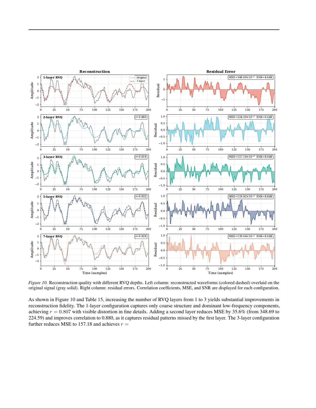
BrainR VQ: A High-Fidelity EEG F oundation Model via Dual-Domain Residual Quantization and Hierar chical A utor egression Mingzhe Cui 1 T ao Chen * 1 2 Y ang Jiao 3 Y iqin W ang 1 Lei Xie 1 Y i Pan 3 Luca Mainardi 2 Abstract Dev eloping foundation models for electroen- cephalography (EEG) remains challenging due to the signal’ s low signal-to-noise ratio and com- plex spectro-temporal non-stationarity . Existing approaches often ov erlook the hierarchical la- tent structure inherent in neural dynamics, lead- ing to suboptimal reconstruction of ﬁne-grained information. In this work, we propose Brain- R VQ, a general-purpose EEG foundation model pre-trained on a large-scale corpus of clinical EEG data. Unlike standard masked modeling, BrainR VQ features a Dual-Domain Residual V ec- tor Quantization (DD-R VQ) tokenizer that dis- entangles temporal wa veforms and spectral pat- terns into hierarchical discrete codes. W e fur- ther introduce a hierarchical autore gressive pre- training objecti ve that learns to reconstruct these codes in a coarse-to-ﬁne manner , utilizing an importance-guided curriculum masking strate gy to prioritize information-rich neural ev ents over background noise. Extensiv e experiments across 8 diverse do wnstream datasets demonstrate that BrainR VQ consistently outperforms state-of-the- art baselines, v alidating its effecti veness in learn- ing rob ust and generalizable neural representa- tions. Our code and model weights are av ailable: https://github .com/keqicmz/BrainR VQ 1. Introduction Electroencephalography (EEG) provides a non-in v asive interface for monitoring millisecond-level neural dynam- ics ( Niedermeyer & da Silva , 2005 ). This high temporal resolution has fueled advancements across di verse domains, 1 State K ey Laboratory of Industrial Control T echnology , Zhe- jiang Univ ersity , Hangzhou, China 2 Department of Electronics, In- formation and Bioengineering, Politecnico di Milano, Milan, Italy 3 Shenzhen Institute of Adv anced T echnology , Chinese Academy of Sciences, Shenzhen, China. Correspondence to: T ao Chen < chentao98@zju.edu.cn > . Pr eprint. F ebruary 20, 2026. ranging from seizure detection ( Shoeb , 2009 ), sleep stag- ing ( Aboalayon et al. , 2016 ), emotion recognition ( Zheng & Lu , 2015 ) and motor imagery classiﬁcation ( Pfurtscheller & Neuper , 2001 ). Howe ver , decoding EEG signals remains a formidable challenge for machine learning due to their inherently lo w signal-to-noise ratios (SNR), complex non- stationarity , and substantial v ariability across subjects ( Lotte et al. , 2007 ). These characteristics, combined with the scarcity of large-scale labeled data, ha ve historically con- strained the de velopment of generalizable EEG decoding models in neuroscience. T o address the labeled data bottleneck, self-supervised learn- ing (SSL) has emer ged as a promising paradigm. Early discriminativ e approaches, such as BENDR ( K ostas et al. , 2021 ), employed contrasti ve learning to extract transferable features from unlabeled recordings. More recently , genera- ti ve approaches inspired by Masked Image Modeling (MIM) and Large Language Models (LLMs) have gained promi- nence. Pioneering works like LaBraM ( Jiang et al. , 2024 ) introduced neural tok enizers to con vert continuous EEG into discrete tokens, enabling BER T -style pre-training. Brain- BER T ( W ang et al. , 2023 ) and Brant ( Zhang et al. , 2023 ) further explored distinct masking strategies and architec- tural designs to capture temporal dependencies. Subsequent efforts have focused on scaling and architectural innova- tions: REVE ( Ouahidi et al. , 2025 ) scaled pre-training to ov er 25,000 subjects, CBraMod ( W ang et al. , 2024b ) pro- posed criss-cross attention to separately model spatial and temporal dependencies. Despite these advances, existing EEG foundation models face critical limitations in representation ﬁdelity . First, most current approaches rely on single-domain tokenization, pro- cessing signals either strictly in the time domain or the frequency domain. While time-domain tokenizers e xcel at capturing transient e vents like epileptic spikes, they often struggle to represent global spectral patterns. Conv ersely , frequency-domain methods capture oscillatory rhythms b ut sacriﬁce temporal precision. Consequently , this single- perspecti ve quantization fails to capture the intricate spectro- temporal coupling of neural dynamics, leading to signiﬁcant information loss and suboptimal reconstruction of complex brain signals. 1 Second, the discretization capacity of existing models re- mains limited. Standard neural tokenizers typically employ single-layer vector quantization to project continuous sig- nals into discrete latent codes. This ﬂat quantization lacks the capacity to encode the high-dimensional v ariability of EEG signals. Drawing inspiration from high-ﬁdelity audio generation, Residual V ector Quantization (R VQ) of fers a robust solution by employing a cascade of codebooks to approximate signals with increasing precision. Ho wever , directly applying R VQ to EEG pre-training is non-trivial. EEG signals exhibit an inherent hierarchy characterized by dominant rhythms and subtle details, yet are signiﬁcantly contaminated by background noise. Standard masked mod- eling objecti ves treat all residual codes independently and equally , which fails to capture the coarse-to-ﬁne semantic dependency and often results in the model wasting capacity on reconstructing background noise rather than meaningful neural ev ents. In this work, we propose BrainR VQ, a high-ﬁdelity EEG foundation model designed to resolve these challenges through Dual-Domain Residual Quantization and Hierar- chical Autoregression. T o ov ercome the information loss caused by single-domain processing, we introduce a Dual- Domain Residual V ector Quantization (DD-R VQ) tokenizer . This module disentangles EEG signals into hierarchical dis- crete codes across both time and frequency domains simulta- neously , ensuring that both ﬁne-grained temporal transients and global spectral oscillations are preserved. Furthermore, to address the limitations of ﬂat quantization and indepen- dent prediction, we propose a Hierarchical Autore gressive Pre-training objective. Instead of predicting tokens inde- pendently , our model learns to reconstruct R VQ codes in a coarse-to-ﬁne manner using teacher forcing, explicitly mod- eling the dependency between layers. This is coupled with an importance-guided curriculum masking strategy , which dynamically prioritizes information-rich re gions, enabling the model to learn robust representations from a cleaner neural manifold. The main contributions of this paper are summarized as follows: • Dual-Domain Residual V ector Quantization (DD- R VQ): W e propose a novel tokenizer that performs hierarchical quantization in both time and frequency domains. This dual-perspecti ve design mitigates the information loss inherent in single-domain approaches, enabling high-ﬁdelity encoding of spectro-temporal dynamics. • Hierarchical A utoregressi ve Pre-training: W e intro- duce a generativ e pre-training objectiv e that models the coarse-to-ﬁne dependency of residual codes. By utilizing teacher forcing to predict ﬁner-grained codes conditioned on coarser priors, the model captures the structural hierarchy of neural signals more ef fectiv ely than standard independent masking. • Importance-Guided Curriculum Masking: W e pro- pose an adaptiv e masking strategy that prioritizes high- information patches based on spectral neural content and temporal signal complexity . This curriculum-based approach effecti vely suppresses background noise, forcing the model to focus on semantically meaningful neural ev ents. • Comprehensi ve V alidation: W e pre-train BrainR VQ on a large-scale corpus of clinical EEG data. Ex- tensiv e experiments across 8 div erse do wnstream datasets—including seizure detection, emotion recog- nition, and sleep staging—validate the superior gener - alization capabilities and advanced performance of our model compared to state-of-the-art baselines. 2. Methodology 2.1. Overview The ov erall framework of BrainR VQ is illustrated in Fig- ure 1 . Our approach consists of three integrated stages designed to learn high-ﬁdelity representations from contin- uous EEG signals. First, input signals are processed by the DD-R VQ tokenizer , which discretizes neural dynamics into hierarchical codes across both temporal and spectral domains. Second, we employ an importance-guided curricu- lum masking strate gy to dynamically select information-rich patches based on spectral neural content and temporal com- plexity . Finally , the masked representations are fed into a T ransformer encoder optimized via a hierarchical autore- gressi ve objectiv e, which reconstructs the discrete codes in a coarse-to-ﬁne manner using teacher forcing. The follo wing subsections detail each component. 2.2. EEG Signal Patching and Pr eprocessing Giv en a raw EEG recording X ∈ R C × T , where C denotes the number of channels and T denotes the number of tempo- ral samples, we segment each channel into non-overlapping patches to enable local feature e xtraction. Speciﬁcally , we apply a sliding windo w of length P without ov erlap to parti- tion each channel into patches, yielding: x = { x c,a ∈ R P | c = 1 , . . . , C, a = 1 , . . . , A } , (1) where A = ⌊ T P ⌋ represents the number of patches per chan- nel, and the total number of patches is | x | = C × A . In our implementation, we set P = 200 corresponding to 1-second windows at 200 Hz sampling rate. The patched signal is reshaped into a 3D tensor X p ∈ R C × A × P , where each ele- ment x c,a represents the a -th temporal segment of channel c . 2 F igur e 1. The overall architectur e of the BrainR VQ framework. (A) DDR VQ for EEG T okenization: The module emplo ys a DDR VQ mechanism to discretize EEG signals. It extracts features simultaneously in time and frequency domains and is optimized via a joint objectiv e of reconstruction and embedding loss. (B) Pre-training Stage: W e introduce a Hierarchical Autoregressi ve Masked Modeling objectiv e. The model learns to predict residual tokens in a coarse-to-ﬁne manner, guided by an Importance-Guided Curriculum Masking strategy that prioritizes hi gh-information regions. (C) Do wnstream Adaptation: The pre-trained encoder serves as a general-purpose feature extractor . 2.3. Dual-Domain Residual V ector Quantization T o construct a semantically rich codebook for EEG signals, we propose a DD-R VQ mechanism that addresses two fun- damental limitations of standard VQ-V AE when applied to neural signals: (1) Domain Incompleteness : process- ing signals solely in the temporal domain fails to capture frequency-speciﬁc features such as alpha rhythms (8–12 Hz) or beta oscillations (13–30 Hz), which are critical for cogni- tiv e state recognition; (2) Quantization Bottleneck : single- layer VQ imposes a hard capacity ceiling, often leading to codebook collapse where only a small subset of codes are utilized, resulting in sev ere information loss. Our DD-R VQ addresses these challenges through three synergistic compo- nents: a shared encoder that e xtracts joint time-frequency embeddings, a residual quantization hierarchy with separate temporal and frequency codebooks, and domain-speciﬁc decoders with complementary reconstruction objectiv es. 2 . 3 . 1 . D U A L - D O M A I N E N C O D I N G EEG signals exhibit fundamentally distinct characteristics across domains. The temporal waveform encodes transient ev ent-related potentials (ERPs) and rapid state transitions, while the frequency spectrum re veals sustained oscillatory patterns tied to cognitiv e processes. T o leverage both repre- sentations, we employ a shared-encoder , dual-branch archi- tecture. Giv en a normalized patch ¯ x c,a ∈ R P , we ﬁrst apply the Discrete Fourier T ransform (DFT) to obtain its spectral representation: X freq [ k ] = P − 1 X n =0 ¯ x c,a [ n ] · e − j 2 πk n P , k = 0 , 1 , . . . , P − 1 , (2) where j denotes the imaginary unit. From the complex- val ued spectrum, we e xtract the amplitude A [ k ] = | X freq [ k ] | and phase ϕ [ k ] = arg ( X freq [ k ]) as reconstruction targets. The temporal patch ¯ x c,a is processed through a shared T rans- former encoder , yielding a uniﬁed latent representation h ∈ R d . This representation is then passed through two parallel Residual V ector Quantizers—a temporal quantizer Q t and a frequency quantizer Q f —producing dual discrete token sequences. The quantized representations are subse- quently decoded by domain-speciﬁc decoders to reconstruct the temporal wav eform and the frequency spectra, respec- tiv ely . This shared-encoder , dual-branch design enables learning uniﬁed representations that capture both transient dynamics and oscillatory structure. 3 2 . 3 . 2 . R E S I D U A L V E C T O R Q UA N T I Z A T I O N : H I E R A R C H I C A L C O A R S E - TO - F I N E D I S C R E T I Z A T I O N Standard single-layer VQ maps each continuous embed- ding to a single discrete code, limiting representational capacity . T o overcome this bottleneck, we employ R VQ, which iterati vely reﬁnes the representation through a hi- erarchy of codebooks { V ( l ) } L l =1 , where each codebook V ( l ) = { v ( l ) k ∈ R d } K l k =1 contains K l code vectors at le vel l . The quantization proceeds recursiv ely: z ( l ) i = arg min k ∈{ 1 ,...,K l } ∥ r ( l − 1) − v ( l ) k ∥ 2 , r ( l ) = r ( l − 1) − v ( l ) z ( l ) i , with r (0) = ˜ e , (3) where r ( l ) denotes the residual after quantization at le vel l , and z ( l ) i ∈ { 1 , . . . , K l } is the selected code inde x. The ﬁnal quantized representation is the sum of all selected codes: h q = L X l =1 v ( l ) z ( l ) i . (4) This hierarchical structure enables coarse-to-ﬁne modeling: the ﬁrst layer captures global patterns, while subsequent layers reﬁne local details. Critically , we maintain separate R VQ branches for temporal and frequenc y domains, denoted as h ( t ) q and h ( f ) q , each producing L token indices per patch: z ( t ) = [ z (1) , . . . , z ( L ) ] and z ( f ) = [ z (1) , . . . , z ( L ) ] . 2 . 3 . 3 . R E C O N S T R U C T I O N T o supervise the learning of meaningful codebooks, we employ three complementary reconstruction objecti ves that enforce consistency across temporal and spectral vie ws. The temporal decoder reconstructs the normalized wav eform from h ( t ) q : L time = ∥ Decoder t ( h ( t ) q ) − ¯ x c,a ∥ 2 2 , (5) encouraging the temporal codebook to preserve the original signal morphology . The frequency decoder reconstructs both amplitude and phase spectra from h ( f ) q : L freq = ∥ y A − A ∥ 2 2 + ∥ y ϕ − ϕ ∥ 2 2 , (6) where y A = Decoder ( A ) f ( h ( f ) q ) and y ϕ = Decoder ( ϕ ) f ( h ( f ) q ) are the predicted amplitude and phase. This dual recon- struction ensures the frequency codebook captures spectral energy distrib ution and phase relationships critical for oscil- latory patterns. The total training objecti ve integrates these reconstruction terms with a commitment loss to regularize the discrete la- tent space. Gi ven the hierarchical nature of our quantization, we enforce the commitment constraint at ev ery residual le vel l . The total loss function is formulated as: L total = L time + L freq + β X d ∈{ t,f } L X l =1 ∥ sg [ r ( l − 1) d ] − v ( l ) d ∥ 2 2 , (7) where sg [ · ] denotes the stop-gradient operator used to pre- vent encoder collapse. The summation term aggregates the quantization errors across all L layers for both temporal and frequency domains, where r ( l − 1) d is the residual input to layer l and v ( l ) d is the selected code vector . By enforcing consistency across temporal w aveforms, amplitude spectra, and phase spectra, this multi-view constraint ensures that the learned tokens encapsulate rich, noise-robust represen- tations of neural dynamics, enabling ef fectiv e downstream transfer . 2.4. Hierarchical A utoregressi ve Pre-training Standard masked autoencoding predicts each token indepen- dently from the same contextualized embedding, discarding the coarse-to-ﬁne structure inherent in R VQ representations. The ﬁrst-layer code z (1) i captures global patterns, which should inform predictions of subsequent codes to reﬁne local details. T o exploit this hierarchy , we design a pre- training frame work that models inter -layer dependencies via autoregressi ve factorization. 2 . 4 . 1 . A U T O R E G R E S S I V E F AC T O R I Z A T I O N Giv en the set of masked patch indices M and visible context X \M , standard approaches formulate the objectiv e as: L MAE = X i ∈M L X l =1 − log P ( z ( l ) i | X \M ) , (8) where each layer’ s token z ( l ) i is predicted independently . This independence assumption ignores the hierarchical prior established during tokenization. T o address this, we factor - ize the joint distribution of all tok ens at position i as: P ( z i | X \M ) = L Y l =1 P ( z ( l ) i | z (1: l − 1) i , X \M ) , (9) where z (1: l − 1) i = [ z (1) i , . . . , z ( l − 1) i ] denotes codes from pre- ceding layers. This formulation ensures that each layer’ s prediction is conditioned on coarser priors, enabling pro- gressiv e reﬁnement from global structure to local detail. Architecturally , we employ a shared T ransformer encoder f θ followed by L layer-speciﬁc prediction heads { g ( l ) θ } L l =1 . T o predict the tok en at layer l , we augment the encoder output with the cumulative embeddings from all preceding 4 layers: ˆ z ( l ) i = g ( l ) θ LN ( l ) h i + l − 1 X k =1 Embed ( k ) ( z ( k ) i ) !! , (10) where h i = f θ ( X \M ) i is the encoder output for position i , Embed ( k ) ( · ) denotes a learnable embedding that maps the discrete code index z ( k ) i to the hidden dimension, and LN ( l ) is a layer-speciﬁc normalization. For the ﬁrst layer ( l = 1 ), no conditioning is applied and the prediction head directly operates on h i . The cumulati ve sum encodes the partial reconstruction from all coarser lev els, providing a progressiv ely reﬁned structural prior . 2 . 4 . 2 . T E A C H E R - F O R C I N G O P T I M I Z A T I O N Direct autoregressiv e training would require sampling ˆ z ( l − 1) i to condition layer l , leading to error accumulation from noisy early-layer predictions. T o stabilize optimization, we employ teacher forcing: during training, we condition on ground-truth codes z (1: l − 1) i obtained from the tokenizer rather than model predictions. The layer-wise loss becomes: L ( l ) = X i ∈M − log P θ ( z ( l ) i | z (1: l − 1) i , X \M ) . (11) The total pre-training objectiv e aggregates losses across all L layers with depth-dependent weights: L HAR = L X l =1 λ l · L ( l ) , (12) where λ l = 2 − ( l − 1) assigns higher importance to coarser layers, as errors in early predictions propagate through the autoregressi ve chain. At inference time, the model operates in a fully autoregressi ve manner: it ﬁrst predicts ˆ z (1) i , re- triev es the corresponding embedding to condition layer 2, and iterates through all L layers, faithfully replicating the generativ e factorization. 2 . 4 . 3 . I M P O RTA N C E - G U I D E D C U R R I C U L U M M A S K I N G Standard masked language modeling employs uniform ran- dom masking, sampling patches with equal probability re- gardless of their information content. While this ensures unbiased coverage, it is suboptimal for physiological sig- nals where informativ e neural ev ents are sparse and tem- porally localized, including epileptic spikes, sleep spindles, and e vent-related potentials. Masking uninformativ e back- ground yields trivial reconstruction tasks, whereas selec- tiv ely masking high-information regions forces the encoder to reason about complex neural dynamics. T o address this, we propose an importance-guided curriculum masking strat- egy that transitions from exploration to e xploitation as train- ing proceeds. Physiology-A ware Importance Scoring. T o quantify the information density of each patch, we design a composite scoring function inte grating frequenc y-domain and time- domain characteristics. In the frequency domain, we com- pute the power spectral density via DFT and extract two metrics: (1) the neural band ratio, measuring power concen- tration within physiologically relev ant bands; and (2) the artifact penalty , quantifying contamination from baseline drift and muscle artifacts. In the time domain, we employ Hjorth parameters, which provide computationally efﬁcient estimates of mean frequency and spectral bandwidth, re- spectiv ely . W e additionally compute an irre gularity metric capturing signal non-stationarity . The ﬁnal importance score aggregates these metrics: S c,a = X m α m · ˜ S m , (13) where ˜ S m denotes the min-max normalized score for met- ric m , and { α m } are weighting coefﬁcients that prioritize neural band content and artifact-free segments. Curriculum via Importance-W eighted Sampling. T o implement curriculum learning, we adopt a probabilistic sampling strategy that balances information-guided selec- tion with stochastic exploration. The combined score for each patch is: ˆ S c,a ( t ) = w ( t ) · S c,a + (1 − w ( t )) · U c,a , (14) where U c,a ∼ Uniform (0 , 1) introduces randomness, and w ( t ) is a curriculum weight that increases linearly during training. Early in training, the sampling distribution is nearly uniform, encouraging broad exploration. As training pro- gresses, the distribution becomes increasingly biased to- ward high-importance patches, forcing the model to focus on information-dense regions. This curriculum strategy improv es both con vergence speed and ﬁnal representation quality by balancing global coverage with focused learning on challenging neural e vents.The detailed formulation of importance scoring metrics is provided in Appendix B . 3. Experiments 3.1. Pre-training Dataset. W e pre-train our model on the lar ge-scale T emple Univ ersity Hospital EEG Corpus (TUEG) ( Obeid & Picone , 2016 ) (v2.0.1). As one of the largest publicly av ailable clinical EEG archives, it comprises 26,846 sessions col- lected from 14,987 unique patients, spanning a cumulati ve duration exceeding 27,000 hours. The corpus exhibits signif- icant real-world heterogeneity , featuring diverse acquisition parameters with sampling rates ranging from 250 Hz to 1024 Hz and over 40 dif fering channel conﬁgurations. This substantial scale and inherent clinical variability provide 5 a robust foundation for learning generalizable neural rep- resentations across di verse physiological and pathological states. Prepr ocessing. W e follo w standard preprocessing protocols to ensure data quality . Recordings shorter than 5 minutes are excluded, and the ﬁrst and last minute of each session are discarded to remove boundary artifacts. W e retain 19 channels conforming to the international 10-20 system (Fp1, Fp2, F7, F3, Fz, F4, F8, T3, C3, Cz, C4, T4, T5, P3, Pz, P4, T6, O1, O2). A band-pass ﬁlter (0.3–75 Hz) is applied to remov e low-frequency drift and high-frequenc y noise, followed by a notch ﬁlter at 60 Hz to suppress po wer line interference. All signals are resampled to 200 Hz and seg- mented into 30-second non-ov erlapping samples. T o further ensure quality , samples containing any data point with ab- solute amplitude exceeding 100 µ V are discarded. Finally , amplitudes are normalized by dividing by 100 µ V . After pre- processing, 1,109,545 samples (approximately 9,200 hours) are retained for pre-training. Implementation Details. W e implemented BrainR VQ us- ing Python 3.10 and PyT orch 2.1.2 + CUD A 11.8. All ex- periments are conducted on NVIDIA A800 (80GB) GPUs. For the DD-R VQ T okenizer , we use a 12-layer T ransformer encoder with embedding dimension 200 and a 3-layer T rans- former decoder . Both temporal and frequency codebooks employ 3-layer R VQ with vocabulary sizes 8192 and embed- ding dimension 64. The DDR VQ is trained for 20 epochs with batch size 128, taking approximately 12 hours on six NVIDIA A800 GPUs. For pre-training, we use a 12-layer T ransformer encoder with hidden dimension 200 and 10 attention heads. Pre-training runs for 20 epochs with batch size 64, taking approximately 20 hours on six NVIDIA A800 GPUs. More details can be found in Appendix C . 3.2. Experimental Setup Downstr eam T asks. W e ev aluate BrainR VQ on a compre- hensiv e suite of 8 downstream datasets spanning diverse BCI application domains, as summarized in T able 1 . For neurological diagnosis, we include TU AB ( Obeid & Pi- cone , 2016 ), TUEV ( Obeid & Picone , 2016 ), and CHB- MIT ( Shoeb , 2009 ). For af fectiv e computing, we adopt the 5-class emotion recognition benchmark SEED-V ( Liu et al. , 2021 ). For motor imagery decoding, we e valuate on PhysioNet ( Schalk et al. , 2004 ), SHU-MI ( Ma et al. ), and BCICIV -2a ( T angermann et al. , 2012 ), cov ering various electrode conﬁgurations and classiﬁcation scenarios. Fi- nally , for cognitive state monitoring, we include the Mental W orkload dataset ( Zyma et al. , 2019 ). This div erse protocol rigorously tests the generalization capability across different recording setups and paradigms. Detailed conﬁgurations are provided in Appendix D . Baselines. W e compare BrainR VQ against two cate- T able 1. Overvie w of the 8 downstream datasets across di verse BCI tasks. T ask Dataset #Ch W in(s) #Samps T ype Abnormal Det. TU AB ( Obeid & Picone , 2016 ) 16 10 409,455 Binary Event Class. TUEV ( Obeid & Picone , 2016 ) 16 5 112,491 6-Class Seizure Det. CHB-MIT ( Shoeb , 2009 ) 16 10 326,993 Binary Emotion Rec. SEED-V ( Liu et al. , 2021 ) 62 1 117,744 5-Class Motor Imagery PhysioNet ( Schalk et al. , 2004 ) 64 4 9,837 4-Class SHU-MI ( Ma et al. ) 32 4 11,988 Binary BCICIV -2a ( T angermann et al. , 2012 ) 22 4 5,088 4-Class W orkload Mental ( Zyma et al. , 2019 ) 20 5 1,707 Binary gories of methods. The ﬁrst includes supervised baselines trained from scratch: EEGNet ( La whern et al. , 2018 ) and ST -Transformer ( Song et al. , 2021 ). The second com- prises self-supervised foundation models pre-trained on large-scale EEG corpora: BENDR ( K ostas et al. , 2021 ), BIO T ( Y ang et al. , 2023 ), LaBraM ( Jiang et al. , 2024 ), and CBraMod ( W ang et al. , 2024b ). All foundation models are pre-trained on the TUH EEG corpus and ﬁne-tuned fol- lowing their ofﬁcial protocols to ensure fair comparison. Implementation details are in Appendix D . Implementation and Metrics. W e adopt Balanced Accu- racy , A UC-PR, and A UR OC for binary classiﬁcation, and Balanced Accuracy , Cohen’ s Kappa, and W eighted F1 for multi-class classiﬁcation. A UR OC and Kappa serve as the monitor scores for model selection, respectively . All results are reported as mean ± standard deviation o ver ﬁ ve random seeds. 3.3. Results T o comprehensively validate the capability and generaliz- ability of BrainR VQ, we ev aluate it against baselines across a di verse suite of eight publicly available BCI datasets. In this section, we focus on four representative do wnstream tasks, listed in T able 2 . In all experiments, we ensure strict consistency in the splits of training, validation, and test sets for ev ery method. The comprehensiv e results on the additional datasets are detailed in Appendix D . Mental W orkload Detection. W e use the Mental W orkload dataset for cogniti ve state assessment. BrainR VQ achiev es state-of-the-art performance on this task. Speciﬁcally , Brain- R VQ obtains a signiﬁcant performance impro vement com- pared to the best baseline CBraMod (0.862 vs. 0.791 in A UROC and 0.758 vs. 0.627 in A UC-PR). The substantial gain in A UC-PR demonstrates that our model excels at dis- tinguishing positi ve samples from negati ve ones across all decision thresholds, which is critical for practical deploy- 6 T able 2. Main e valuation results on four representative do wnstream tasks. The table is divided into binary classiﬁcation (top) and multi-class classiﬁcation (bottom). Best results are in bold , second best are underlined. Method Mental W orkload CHB-MIT Bal. Acc A UC-PR A UR OC Bal. Acc A UC-PR A UR OC EEGNet 0.677 ± 0.012 0.576 ± 0.010 0.732 ± 0.011 0.566 ± 0.011 0.191 ± 0.018 0.805 ± 0.014 ST -Transformer 0.663 ± 0.017 0.567 ± 0.026 0.713 ± 0.017 0.592 ± 0.020 0.142 ± 0.009 0.824 ± 0.049 BENDR 0.568 ± 0.045 0.366 ± 0.067 0.568 ± 0.045 0.561 ± 0.043 0.307 ± 0.124 0.863 ± 0.053 BIO T 0.688 ± 0.019 0.600 ± 0.020 0.754 ± 0.014 0.707 ± 0.046 0.328 ± 0.046 0.876 ± 0.028 LaBraM 0.691 ± 0.013 0.600 ± 0.016 0.772 ± 0.009 0.708 ± 0.036 0.329 ± 0.040 0.868 ± 0.020 CBraMod 0.726 ± 0.013 0.627 ± 0.010 0.791 ± 0.007 0.740 ± 0.028 0.369 ± 0.038 0.889 ± 0.015 BrainR VQ (Ours) 0.747 ± 0.011 0.758 ± 0.012 0.862 ± 0.010 0.709 ± 0.040 0.465 ± 0.036 0.928 ± 0.024 Method TUEV BCICIV -2a Bal. Acc Kappa W -F1 Bal. Acc Kappa W -F1 EEGNet 0.388 ± 0.014 0.358 ± 0.016 0.654 ± 0.012 0.448 ± 0.009 0.269 ± 0.012 0.423 ± 0.011 ST -Transformer 0.398 ± 0.023 0.377 ± 0.031 0.682 ± 0.019 0.458 ± 0.015 0.273 ± 0.020 0.447 ± 0.014 BENDR 0.436 ± 0.025 0.427 ± 0.024 0.676 ± 0.022 0.490 ± 0.007 0.320 ± 0.009 0.484 ± 0.007 BIO T 0.528 ± 0.023 0.527 ± 0.025 0.749 ± 0.008 0.475 ± 0.009 0.300 ± 0.014 0.461 ± 0.013 LaBraM 0.641 ± 0.007 0.664 ± 0.009 0.831 ± 0.005 0.487 ± 0.009 0.316 ± 0.015 0.476 ± 0.010 CBraMod 0.667 ± 0.011 0.677 ± 0.010 0.834 ± 0.006 0.514 ± 0.007 0.352 ± 0.009 0.498 ± 0.009 BrainR VQ (Ours) 0.668 ± 0.015 0.690 ± 0.008 0.840 ± 0.005 0.541 ± 0.008 0.388 ± 0.008 0.533 ± 0.012 ment in human-machine interaction systems. Seizure Detection. CHB-MIT is a highly imbalanced clinical dataset for pediatric seizure detection. BrainR VQ achiev es the best performance on ranking metrics, obtain- ing 0.928 in A UR OC and 0.465 in A UC-PR, compared to the best baseline CBraMod (0.889 in A UR OC and 0.369 in A UC-PR). The remarkable 26.0% relative impro vement in A UC-PR indicates that our importance-guided curriculum masking effecti vely forces the model to attend to sparse but discriminati ve ictal patterns rather than the dominant interictal background. Event T ype Classiﬁcation. TUEV is a challenging 6-class clinical ev ent classiﬁcation task from the T emple Uni versity Hospital corpus. BrainR VQ achiev es the best performance on all metrics. Speciﬁcally , BrainR VQ obtains a Cohen’ s Kappa of 0.690, surpassing the best baseline CBraMod (0.677 in Kappa). This improvement demonstrates the ef- fectiv eness of our hierarchical autoregressi ve pre-training in capturing di verse clinical EEG patterns including spik e- and-wa ve complex es, generalized periodic discharges, and artifact signatures. Motor Imagery Classiﬁcation. W e use BCICIV -2a for e val- uation on 4-class motor imagery classiﬁcation. BrainR VQ achiev es a signiﬁcant performance gain compared to the best baseline CBraMod (0.388 vs. 0.352 in Cohen’ s Kappa and 0.533 vs. 0.498 in W eighted F1). This 10.2% relati ve improv ement in Kappa demonstrates that our Dual-Domain R VQ effecti vely captures both the transient event-related desynchronization and the sustained sensorimotor rhythms T able 3. Ablation study results. A UROC for binary and Cohen’ s Kappa for multi-class tasks. Conﬁguration Binary (A UR OC ↑ ) Multi-class (Kappa ↑ ) Mental CHB-MIT TUEV BCICIV -2a Full Model 0.862 0.928 0.690 0.388 (a) Dual-Domain T oken. w/o Freq codebook 0.845 0.887 0.639 0.373 w/o T ime codebook 0.857 0.896 0.655 0.374 (b) Residual Quant. Single-layer VQ 0.849 0.896 0.682 0.321 (c) Hierar chical A utoReg . Independent pred. 0.780 0.875 0.662 0.335 (d) Masking Random masking 0.852 0.910 0.673 0.363 that characterize motor intention, which single-domain tok- enizers tend to conﬂate. 3.4. Ablation Study T o v alidate the efﬁcacy of each component in our proposed framew ork, we conducted comprehensi ve ablation studies across four di verse datasets: Mental W orkload, CHB-MIT , TUEV , and BCICIV -2a. The quantitative results are summa- rized in T able 3 , with corresponding visualizations pro vided in Figure 2 . More comprehensi ve ablation results are pro- vided in Appendix F and Appendix E . 7 Mental W orkload CHB-MIT 0.70 0.75 0.80 0.85 0.90 0.95 1.00 AUROC 0.862 0.928 0.845 0.887 0.857 0.896 0.849 0.896 0.780 0.875 0.852 0.910 TUEV B CICIV -2a 0.3 0.4 0.5 0.6 0.7 Cohen's K appa 0.690 0.388 0.639 0.373 0.655 0.374 0.682 0.321 0.662 0.335 0.673 0.363 F ull Model w/o F r eq w/o T ime Single VQ Independent R andom Mask F igur e 2. V isualization of ablation study results. The proposed Full Model (dark blue) consistently outperforms single-domain and non-hierarchical variants across all datasets. Left: A UROC scores for Mental W orkload and CHB-MIT . Right: Cohen’ s Kappa scores for TUEV and BCICIV -2a. Effectiveness of Dual-Domain T okenization. The remov al of either the temporal or frequency codebook results in consistent performance deterioration, underscoring the com- plementary nature of these two representations. Speciﬁ- cally , the frequency-only variant (w/o Time) retains com- petitiv e performance on Mental W orkload ( ∆ 0.6%) and CHB-MIT ( ∆ 3.4%), suggesting that cogniti ve states and seizure anomalies are primarily characterized by spectral power shifts. Con versely , the temporal-only variant (w/o Freq) suf fers a more signiﬁcant drop on TUEV ( ∆ 7.4%), where clinical e vent classiﬁcation relies heavily on wa ve- form morphology . The superiority of the full DD-R VQ across all tasks v alidates our design of jointly modeling time-frequency dynamics. Impact of Residual Quantization. Collapsing our 3-layer R VQ into a standard single-layer VQ yields an average per - formance decline of 5.9%. This degradation is particularly pronounced on BCICIV -2a ( ∆ 17.3%), a task requiring the discrimination of ﬁne-grained motor imagery signals. W e hypothesize that the hierarchical residual codes naturally capture the multi-scale structure of neural dynamics: coarse layers encode general intent, while ﬁne layers resolve subtle class differences. These results conﬁrm that residual quanti- zation provides the necessary representational granularity for complex EEG decoding. Necessity of Hierarchical A utoregression. W e replaced the hierarchical autoregressiv e predictor with an indepen- dent prediction mechanism—where all codebook layers are predicted simultaneously without conditioning on coarser codes. This modiﬁcation causes a substantial 8.3% a ver- age degradation, with se vere impacts on Mental W orkload ( ∆ 9.5%) and BCICIV -2a ( ∆ 13.7%). This ﬁnding conﬁrms that explicitly modeling coarse-to-ﬁne dependencies guides the encoder to learn more structured and semantically rich representations, which is critical for do wnstream tasks in- volving subtle signal v ariations. Beneﬁt of information Masking . Ablating the importance- guided curriculum masking in fav or of uniform random masking leads to a 3.0% drop in a verage performance. The impact is most signiﬁcant on the data-scarce BCICIV - 2a dataset ( ∆ 6.4%). This validates that prioritizing information-rich neural events during pre-training signiﬁ- cantly improves data ef ﬁciency and transferability , enabling the model to learn robust features e ven from limited data. 4. Conclusion In this work, we presented BrainR VQ, a high-ﬁdelity EEG foundation model that uniﬁes temporal and spectral mod- eling through DD-R VQ. By integrating hierarchical autore- gressiv e pre-training with importance-guided curriculum masking, our framew ork effecti vely captures the coarse- to-ﬁne structure of complex neural dynamics. Extensive experiments across eight di verse benchmarks demonstrate that BrainR VQ consistently outperforms state-of-the-art baselines, exhibiting rob ust generalization in seizure de- tection, motor imagery , and BCI tasks. W e belie ve Brain- R VQ provides a strong foundation for de veloping practical BCI systems and clinical EEG analysis tools. Future work includes scaling to larger models and incorporating multi- 8 modal physiological signals. Impact Statement This work contributes to the adv ancement of machine learn- ing for physiological signal processing. By de veloping ro- bust foundation models for EEG, our research has the poten- tial to accelerate the dev elopment of more accurate clinical diagnostic tools and efﬁcient assistive neurotechnologies, ultimately beneﬁting healthcare and human-machine inter- action domains. References Aboalayon, K. A. I., F aezipour, M., Almuhammadi, W . S., and Moslehpour , S. Sleep stage classiﬁcation using eeg signal analysis: a comprehensive surv ey and new in vesti- gation. Entr opy , 18(9):272, 2016. Achiam, J., Adler , S., Agarwal, S., Ahmad, L., Akkaya, I., Aleman, F . L., Almeida, D., Altenschmidt, J., Altman, S., Anadkat, S., et al. Gpt-4 technical report. arXiv preprint arXiv:2303.08774 , 2023. Bashashati, A., Fatourechi, M., W ard, R. K., and Birch, G. E. A surv ey of signal processing algorithms in brain– computer interfaces based on electrical brain signals. Journal of Neur al engineering , 4(2):R32, 2007. Borsos, Z., Marinier, R., V incent, D., Kharitono v , E., Pietquin, O., Shariﬁ, M., Roblek, D., T eboul, O., Grang- ier , D., T agliasacchi, M., et al. Audiolm: a language modeling approach to audio generation. IEEE/ACM trans- actions on audio, speech, and language pr ocessing , 31: 2523–2533, 2023. Craik, A., He, Y ., and Contreras-V idal, J. L. Deep learning for electroencephalogram (eeg) classiﬁcation tasks: a revie w . Journal of neur al engineering , 16(3):031001, 2019. D ´ efossez, A., Copet, J., Synnaeve, G., and Adi, Y . High ﬁdelity neural audio compression. arXiv pr eprint arXiv:2210.13438 , 2022. Devlin, J., Chang, M.-W ., Lee, K., and T outanova, K. Bert: Pre-training of deep bidirectional transformers for lan- guage understanding. In Pr oceedings of the 2019 confer- ence of the North American chapter of the association for computational linguistics: human language tec hnologies, volume 1 (long and short papers) , pp. 4171–4186, 2019. He, K., Chen, X., Xie, S., Li, Y ., Doll ´ ar , P ., and Girshick, R. Mask ed autoencoders are scalable vision learners. In Pr oceedings of the IEEE/CVF conference on computer vision and pattern r ecognition , pp. 16000–16009, 2022. Jiang, W .-B., Zhao, L.-M., and Lu, B.-L. Lar ge brain model for learning generic representations with tremendous ee g data in bci. arXiv pr eprint arXiv:2405.18765 , 2024. K ostas, D., Aroca-Ouellette, S., and Rudzicz, F . Bendr: Us- ing transformers and a contrasti ve self-supervised learn- ing task to learn from massi ve amounts of ee g data. F r on- tiers in Human Neur oscience , 15:653659, 2021. Langley , P . Crafting papers on machine learning. In Langley , P . (ed.), Pr oceedings of the 17th International Confer ence on Machine Learning (ICML 2000) , pp. 1207–1216, Stan- ford, CA, 2000. Morgan Kaufmann. Lawhern, V . J., Solon, A. J., W aytowich, N. R., Gordon, S. M., Hung, C. P ., and Lance, B. J. Ee gnet: a com- pact conv olutional neural network for eeg-based brain– computer interfaces. Journal of neur al engineering , 15 (5):056013, 2018. Lee, Y .-E. and Lee, S.-H. Eeg-transformer: Self-attention from transformer architecture for decoding ee g of imag- ined speech. In 2022 10th International winter conference on brain-computer interface (BCI) , pp. 1–4. IEEE, 2022. Liu, W ., Qiu, J.-L., Zheng, W .-L., and Lu, B.-L. Comparing recognition performance and robustness of multimodal deep learning models for multimodal emotion recogni- tion. IEEE T ransactions on Co gnitive and Developmental Systems , 14(2):715–729, 2021. Lotte, F ., Congedo, M., L ´ ecuyer , A., Lamarche, F ., and Arnaldi, B. A revie w of classiﬁcation algorithms for eeg-based brain–computer interf aces. J ournal of neural engineering , 4(2):R1, 2007. Ma, J., Y ang, B., Qiu, W ., Li, Y ., Gao, S., and Xia, X. A large ee g dataset for studying cross-session variability in motor imagery brain-computer interface. scientiﬁc data, 2022, 9 (1). Ma, J., W u, F ., Lin, Q., Xing, Y ., Liu, C., Jia, Z., and Feng, M. Codebrain: Bridging decoupled tokenizer and multi-scale architecture for eeg foundation model. arXiv pr eprint arXiv:2506.09110 , 2025. Ma, Y ., Song, Y ., and Gao, F . A nov el hybrid cnn- transformer model for eeg motor imagery classiﬁcation. In 2022 International joint confer ence on neural networks (IJCNN) , pp. 1–8. IEEE, 2022. Niedermeyer , E. and da Silv a, F . L. Electr oencephalography: basic principles, clinical applications, and r elated ﬁelds . Lippincott W illiams & W ilkins, 2005. Obeid, I. and Picone, J. The temple uni versity hospital ee g data corpus. F r ontiers in neur oscience , 10:196, 2016. 9 Ouahidi, Y . E., L ys, J., Th ¨ olke, P ., Farrugia, N., Pasde- loup, B., Gripon, V ., Jerbi, K., and Lioi, G. Rev e: A foundation model for eeg–adapting to any setup with large-scale pretraining on 25,000 subjects. arXiv pr eprint arXiv:2510.21585 , 2025. Pfurtscheller , G. and Neuper , C. Motor imagery and direct brain-computer communication. Pr oceedings of the IEEE , 89(7):1123–1134, 2001. Roy , Y ., Ban ville, H., Albuquerque, I., Gramfort, A., Falk, T . H., and Faubert, J. Deep learning-based electroen- cephalography analysis: a systematic revie w . J ournal of neural engineering , 16(5):051001, 2019. Schalk, G., McFar land, D. J., Hinterberger , T ., Birbaumer , N., and W olpaw , J. R. Bci2000: a general-purpose brain- computer interface (bci) system. IEEE T ransactions on biomedical engineering , 51(6):1034–1043, 2004. Schirrmeister , R. T ., Springenberg, J. T ., Fiederer , L. D. J., Glasstetter , M., Eggensperger , K., T angermann, M., Hut- ter , F ., Burgard, W ., and Ball, T . Deep learning with con volutional neural networks for eeg decoding and vi- sualization. Human brain mapping , 38(11):5391–5420, 2017. Shoeb, A. H. Application of machine learning to epilep- tic seizure onset detection and tr eatment . PhD thesis, Massachusetts Institute of T echnology , 2009. Song, Y ., Jia, X., Y ang, L., and Xie, L. T ransformer-based spatial-temporal feature learning for eeg decoding. arXiv pr eprint arXiv:2106.11170 , 2021. Supratak, A., Dong, H., W u, C., and Guo, Y . Deepsleepnet: A model for automatic sleep stage scoring based on ra w single-channel eeg. IEEE transactions on neural systems and r ehabilitation engineering , 25(11):1998–2008, 2017. T angermann, M., M ¨ uller , K.-R., Aertsen, A., Birbaumer , N., Braun, C., Brunner , C., Leeb, R., Mehring, C., Miller, K. J., M ¨ uller-Putz, G. R., et al. Re view of the bci compe- tition iv . F r ontiers in neur oscience , 6:55, 2012. V an Den Oord, A., V inyals, O., et al. Neural discrete rep- resentation learning. Advances in neural information pr ocessing systems , 30, 2017. W ang, C., Subramaniam, V ., Y aari, A. U., Kreiman, G., Katz, B., Cases, I., and Barbu, A. Brainbert: Self- supervised representation learning for intracranial record- ings. arXiv pr eprint arXiv:2302.14367 , 2023. W ang, G., Liu, W ., He, Y ., Xu, C., Ma, L., and Li, H. Eegpt: Pretrained transformer for uni versal and reliable repre- sentation of eeg signals. Advances in Neural Information Pr ocessing Systems , 37:39249–39280, 2024a. W ang, J., Zhao, S., Luo, Z., Zhou, Y ., Jiang, H., Li, S., Li, T ., and Pan, G. Cbramod: A criss-cross brain foundation model for eeg decoding. arXiv pr eprint arXiv:2412.07236 , 2024b. W iggins, W . F . and T ejani, A. S. On the opportunities and risks of foundation models for natural language process- ing in radiology . Radiology: Artiﬁcial Intelligence , 4(4): e220119, 2022. Y ang, C., W estover , M., and Sun, J. Biot: Biosignal trans- former for cross-data learning in the wild. Advances in Neural Information Pr ocessing Systems , 36:78240– 78260, 2023. Zeghidour , N., Luebs, A., Omran, A., Skoglund, J., and T agliasacchi, M. Soundstream: An end-to-end neural audio codec. IEEE/A CM T ransactions on Audio, Speec h, and Language Pr ocessing , 30:495–507, 2021. Zhang, D., Y uan, Z., Y ang, Y ., Chen, J., W ang, J., and Li, Y . Brant: Foundation model for intracranial neural signal. Advances in Neural Information Pr ocessing Systems , 36: 26304–26321, 2023. Zheng, W .-L. and Lu, B.-L. In vestig ating critical frequenc y bands and channels for eeg-based emotion recognition with deep neural networks. IEEE T ransactions on au- tonomous mental development , 7(3):162–175, 2015. Zyma, I., T ukaev , S., Seleznov , I., Kiyono, K., Popov , A., Chernykh, M., and Shpenkov , O. Electroencephalograms during mental arithmetic task performance. Data , 4(1): 14, 2019. 10 A. Related W ork A.1. EEG Decoding Methods EEG is a non-in vasi ve technique to measure brain acti vity . Early studies on EEG decoding predominantly emplo yed traditional machine learning methods ( Bashashati et al. , 2007 ; Lotte et al. , 2007 ), which usually depend on hand-crafted features that require extensi ve prior knowledge and often e xhibit weak generalizability . W ith the de velopment of deep learning techniques, an increasing number of researchers have shifted their focus to studying EEG decoding methods based on deep learning ( Craik et al. , 2019 ; Roy et al. , 2019 ). Con volutional neural networks (CNNs) have been widely adopted to extract temporal and spatial features from EEG for v arious BCI tasks, including motor imagery classiﬁcation, emotion recognition, and seizure detection ( Schirrmeister et al. , 2017 ; La whern et al. , 2018 ). Long Short-T erm Memory (LSTM) networks have also been employed for EEG feature extraction and classiﬁcation on tasks such as motor imagery and sleep staging ( Supratak et al. , 2017 ). Transformer architectures hav e been utilized to learn spatial-temporal features for BCI tasks including emotion recognition, sleep staging, and person identiﬁcation ( Song et al. , 2021 ; Lee & Lee , 2022 ). T o combine the strengths of CNN and T ransformer , some works de vise CNN-Transformer h ybrid networks for EEG classiﬁcation ( Ma et al. , 2022 ). A.2. EEG Foundation Models Foundation models ( Wiggins & T ejani , 2022 ), such as BER T ( De vlin et al. , 2019 ), MAE ( He et al. , 2022 ), and GPT - 4 ( Achiam et al. , 2023 ), hav e achiev ed remarkable success in computer vision and natural language processing. Howe ver , the potential of foundation models for brain signals remains largely une xplored. Recent efforts ha ve begun to address this gap. BENDR ( K ostas et al. , 2021 ) employs contrastive self-supervised learning to learn generic EEG representations, addressing the problem of limited labeled data. BrainBER T ( W ang et al. , 2023 ) is a pre-training model for intracranial recordings that learns complex non-linear transformations through masked spectrogram modeling. Brant ( Zhang et al. , 2023 ) proposes a foundation model for intracranial neural signals that captures long-term dependencies and spatial correlations across channels. BIO T ( Y ang et al. , 2023 ) introduces a generic biosignal learning model that enables joint pre-training and knowledge transfer across different biosignal datasets. LaBraM ( Jiang et al. , 2024 ) presents a large brain model that learns generic EEG representations by predicting neural tokens of masked EEG patches through a VQ-V AE-based tokenizer . EEGPT ( W ang et al. , 2024a ) proposes a mask-based dual self-supervised learning method for ef ﬁcient feature extraction. CBraMod ( W ang et al. , 2024b ) introduces criss-cross attention to separately model spatial and temporal dependencies. CodeBrain ( Ma et al. , 2025 ) explores state-space models with dual-domain tokenization for EEG representation learning. Despite these adv ances, existing approaches often rely on single-domain tokenization and ﬂat vector quantization, limiting their ability to capture the hierarchical structure of neural dynamics. Our work addresses these limitations through dual-domain residual vector quantization and hierarchical autore gressive pre-training. A.3. V ector Quantization in Neural Signal Processing V ector Quantization (VQ) has emerged as a po werful technique for learning discrete representations of continuous signals. VQ-V AE ( V an Den Oord et al. , 2017 ) introduced the concept of learning discrete latent codes through vector quantization, enabling effecti ve compression and generation of comple x data. R VQ ( Zeghidour et al. , 2021 ) extends this approach by employing a cascade of codebooks to progressively reﬁne the representation. This hierarchical quantization has proven particularly effecti ve in high-ﬁdelity audio generation, as demonstrated by SoundStream ( Zeghidour et al. , 2021 ), EnCodec ( D ´ efossez et al. , 2022 ), and AudioLM ( Borsos et al. , 2023 ). In the context of EEG, LaBraM ( Jiang et al. , 2024 ) ﬁrst introduced neural tokenizers for discretizing EEG signals, but employed single-layer VQ in the time domain only . Our DD-R VQ approach extends this by performing hierarchical quantization in both time and frequency domains, enabling more comprehensive capture of spectro-temporal neural dynamics. 11 B. Preliminaries B.1. Codebook Learning with Exponential Moving A verage T o ensure stable codebook learning and pre vent mode collapse, we employ Exponential Mo ving A verage (EMA) updates for the codebook vectors instead of gradient-based optimization. For each codebook V ( l ) = { v ( l ) k } K k =1 at le vel l , the update rule at training step t is: n ( t ) k = γ · n ( t − 1) k + (1 − γ ) · X i 1 [ z ( l ) i = k ] (15) m ( t ) k = γ · m ( t − 1) k + (1 − γ ) · X i : z ( l ) i = k e i (16) v ( l ) k ← m ( t ) k n ( t ) k + ϵ (17) where γ = 0 . 99 is the decay rate, n k tracks the e xponential moving count of assignments to code k , m k tracks the exponential mo ving sum of assigned embeddings, and ϵ = 10 − 6 prev ents division by zero. This EMA approach provides sev eral advantages: • Stability : Gradual updates prev ent abrupt codebook changes that can destabilize training. • Utilization : Combined with ℓ 2 -normalization of embeddings before quantization, EMA encourages uniform codebook utilization. • Efﬁciency : No gradient computation is required for codebook updates. Additionally , we apply ℓ 2 -normalization to both encoder outputs and codebook vectors before computing distances: ˜ e ← ˜ e ∥ ˜ e ∥ 2 , v k ← v k ∥ v k ∥ 2 (18) This normalization projects all vectors onto a unit hypersphere, making the codebook learning purely directional and improving training stability . B.2. Discrete F ourier T ransform f or EEG Analysis Giv en an EEG patch x ∈ R P , the Discrete Fourier T ransform (DFT) computes its spectral representation: X [ k ] = P − 1 X n =0 x [ n ] · e − j 2 πk n P , k = 0 , 1 , . . . , P − 1 (19) From the complex-v alued spectrum, we extract amplitude and phase: A [ k ] = | X [ k ] | = p Re ( X [ k ]) 2 + Im ( X [ k ]) 2 (20) ϕ [ k ] = arg( X [ k ]) = arctan  Im ( X [ k ]) Re ( X [ k ])  (21) The amplitude spectrum captures the power distrib ution across frequency bands (e.g., delta: 0.5-4 Hz, theta: 4-8 Hz, alpha: 8-13 Hz, beta: 13-30 Hz), while the phase spectrum encodes temporal relationships critical for neural synchronization patterns. B.3. Physiology-A ware Importance Scoring This section provides the detailed formulation of the importance scoring function used in our curriculum masking strate gy . 12 B . 3 . 1 . F R E Q U E N C Y - D O M A I N M E T R I C S Giv en a patch ¯ x c,a ∈ R P , we ﬁrst compute its power spectral density via the Discrete F ourier T ransform: P [ k ] = | X [ k ] | 2 , k = 0 , 1 , . . . , ⌊ P / 2 ⌋ (22) where X [ k ] is the DFT coefﬁcient at frequenc y bin k . The corresponding frequency for each bin is f k = k · f s /P , where f s is the sampling rate. The neural band ratio measures the proportion of power within ph ysiologically relev ant frequency bands: S neural = P k : f k ∈ [4 , 30) Hz P [ k ] P k P [ k ] + ϵ (23) This range encompasses theta (4–8 Hz), alpha (8–13 Hz), and beta (13–30 Hz) rhythms, which are strongly associated with cognitiv e processes and clinical biomarkers. The artifact penalty quantiﬁes contamination from non-neural sources: S clean = 1 − P k : f k < 2 Hz ∨ f k ≥ 45 Hz P [ k ] P k P [ k ] + ϵ (24) Low-frequenc y components ( < 2 Hz) typically reﬂect baseline drift and electrode artifacts, while high-frequenc y components ( ≥ 45 Hz) often correspond to electromyographic (muscle) contamination. B . 3 . 2 . T I M E - D O M A I N M E T R I C S V I A H J O RT H P A R A M E T E R S Hjorth parameters ( ? ) provide computationally efﬁcient estimates of signal dynamics. Let ∆ ¯ x [ p ] = ¯ x [ p ] − ¯ x [ p − 1] and ∆ 2 ¯ x [ p ] = ∆ ¯ x [ p ] − ∆ ¯ x [ p − 1] denote the ﬁrst and second-order dif ferences. The activity parameter captures signal v ariance: S activity = log( V ar ( ¯ x c,a ) + ϵ ) (25) The logarithmic transformation reduces sensiti vity to high-amplitude artifacts. The mobility parameter approximates the mean frequency: S mobility = s V ar (∆ ¯ x c,a ) V ar ( ¯ x c,a ) + ϵ (26) The complexity parameter measures spectral bandwidth: S complexity = 1 S mobility + ϵ s V ar (∆ 2 ¯ x c,a ) V ar (∆ ¯ x c,a ) + ϵ (27) High complexity indicates rich multi-frequency content, whereas low values correspond to narrow-band or monotonic signals. B . 3 . 3 . I R R E G U L A R I T Y M E T R I C T o capture non-stationarity , we compute an irregularity metric based on the v ariability of signal changes: S irreg = E [ | ∆ | ∆ ¯ x c,a || ] E [ | ∆ ¯ x c,a | ] + ϵ (28) This measures how consistently the signal changes o ver time, with higher values indicating more irre gular (and potentially more informativ e) patterns. 13 B . 3 . 4 . S C O R E A G G R E G A T I O N The ﬁnal importance score aggregates all metrics via weighted combination: S c,a = α 1 ˜ S neural + α 2 ˜ S clean + α 3 ˜ S complexity + α 4 ˜ S irreg + α 5 ˜ S mobility (29) where ˜ S m denotes min-max normalization across all patches within a sample. In our implementation, we use α 1 = 0 . 30 , α 2 = 0 . 25 , α 3 = 0 . 20 , α 4 = 0 . 15 , and α 5 = 0 . 10 , prioritizing neural band content and artifact-free segments. B . 3 . 5 . C U R R I C U L U M W E I G H T S C H E D U L E The curriculum weight w ( t ) controls the balance between importance-guided and random masking: w ( t ) = w 0 + ( w max − w 0 ) · t T total (30) W e set w 0 = 0 . 2 and w max = 0 . 7 , ensuring that early training e xplores div erse patches while later training focuses on information-rich regions. The temperature parameter for softmax sampling is set to τ = 0 . 8 . C. Pre-training Analysis This section provides a detailed analysis of the pre-training process for BrainR VQ. W e ﬁrst present the complete hyper- parameter conﬁgurations for reproducibility . Then, we analyze the training dynamics, including loss con ver gence curves and codebook utilization patterns for both the DD-R VQ tokenizer and hierarchical autoregressi ve pre-training stages. Interpretability analysis and qualitativ e visualizations of the learned representations are provided separately . C.1. Pre-training Settings Here we provide complete hyperparameter conﬁgurations for both the DD-R VQ tokenizer and hierarchical autoregressi ve pre-training stages in T able 4 . C.2. T raining Dynamics W e analyze the con ver gence behavior of both training stages to provide insights into the learning process of BrainR VQ. DD-R VQ T okenizer T raining. Figure 3 sho ws the loss curv es during DD-R VQ training. The total loss comprises three reconstruction objectiv es: time-domain wa veform, frequency-domain amplitude, and phase reconstruction. W e observ e rapid con ver gence during the ﬁrst 20 epochs, followed by gradual stabilization. Among the three components, amplitude reconstruction con ver ges fastest due to the relativ ely smooth and predictable nature of spectral po wer distributions. Time- domain reconstruction exhibits slo wer conv ergence, reﬂecting the higher complexity of raw w aveform modeling. Phase reconstruction shows higher variance throughout training, consistent with ﬁndings in audio processing where phase is inherently more challenging to reconstruct than magnitude ( Zeghidour et al. , 2021 ). 0 5 10 15 20 25 Epoch 0.20 0.25 0.30 0.35 0.40 0.45 0.50 0.55 0.60 Time Reconstruction Loss (a) 0 5 10 15 20 25 Epoch 0.1 0.2 0.3 0.4 0.5 Amplitude Reconstruction Loss (b) 0 5 10 15 20 25 Epoch 0.60 0.65 0.70 0.75 0.80 0.85 Phase Reconstruction Loss (c) F igur e 3. DD-R VQ tokenizer training dynamics. The total loss (black) comprises time-domain wa veform reconstruction (blue), frequency- domain amplitude reconstruction (orange), and phase reconstruction (green). Hierarchical A utoregressi ve Pre-training . W e examine both loss curv es (Figure 4 ) and prediction accuracy (Figure 5 ) during pre-training to validate our hierarchical design. As shown in Figure 4 , we observe distinct conv ergence patterns 14 T able 4. Hyperparameters for BrainR VQ pre-training. Hyperparameters T okenizer Pre-training EEG Sample Channels 19 T ime points 6000 (30 seconds @ 200 Hz) Patch dimension 200 (1 second) Sequence length 19 × 30 = 570 Mask ratio – 0.5 Mask token – Learnable P atch Encoder (3-layer 2D T emporal Con v) Input channels { 1, 8, 8 } Output channels { 8, 8, 8 } Kernel size { (1,15), (1,3), (1,3) } Stride { (1,8), (1,1), (1,1) } Padding { (0,7), (0,1), (0,1) } Residual V ector Quantization (per domain) R VQ layers 3 – Codebook sizes [8192, 8192, 8192] – Code embedding dimension 64 – EMA decay 0.99 – Commitment weight ( β ) 1.0 – T ransformer Encoder Layers 12 12 Hidden dimension 200 200 Attention heads 10 10 Feed-forward dimension 800 800 Drop path rate 0.0 0.1 T ransformer Decoder Layers 3 – Hidden dimension 200 – Attention heads 10 – Importance-Guided Masking Softmax temperature ( τ ) – 0.8 Final importance weight – 0.7 Symmetric loss – T rue T raining Epochs 20 20 Batch size 128 64 Optimizer AdamW AdamW Learning rate 5 × 10 − 4 5 × 10 − 4 Adam β (0.9, 0.999) (0.9, 0.999) Adam ϵ 1 × 10 − 8 1 × 10 − 8 W eight decay 5 × 10 − 2 5 × 10 − 2 Scheduler CosineAnnealingLR CosineAnnealingLR W armup epochs 5 5 Minimal learning rate 1 × 10 − 5 1 × 10 − 5 15 across R VQ layers: Layer-0 prediction loss is consistently lo wer than Layer-1 and Layer-2, conﬁrming that coarse codes capturing global patterns (e.g., dominant frequency bands, o verall amplitude en velope) are easier to predict than ﬁne-grained residual codes. The stable loss gap between adjacent layers after warmup validates our layer-wise weighting scheme ( λ 0 > λ 1 > λ 2 ). 0 2 4 6 8 10 12 14 16 18 20 Epoch 25 30 35 40 45 50 55 60 Loss F igur e 4. Pre-training loss dynamics. Layer-0 (coarse) achie ves consistently lower loss than Layer-1/2 (ﬁne), v alidating the coarse-to-ﬁne learning hierarchy . Figure 5 further corroborates this observation from the accuracy perspectiv e. Layer -0 achiev es the highest prediction accuracy of approximately 29%, while Layer-1 and Layer -2 reach 22% and 14%, respecti vely . This monotonic decrease in accuracy across layers aligns with our intuition: coarse-level codes encode dominant signal characteristics that exhibit stronger temporal dependencies and are thus more predictable, whereas ﬁne-lev el residual codes capture high-frequency details and noise-lik e components that are inherently harder to anticipate. Notably , all layers sho w rapid impro vement within the ﬁrst 5 epochs before gradually stabilizing, indicating efﬁcient learning of the hierarchical tok en structure. 0 2 4 6 8 10 12 14 16 18 20 Epoch 0.00 0.05 0.10 0.15 0.20 0.25 0.30 Accuracy Layer 0 Layer 1 Layer 2 F igur e 5. Layer-wise token prediction accurac y during pre-training. Layer-0 achie ves the highest accuracy ( ∼ 29%), followed by Layer -1 ( ∼ 22%) and Layer-2 ( ∼ 14%), conﬁrming that coarse codes are more predictable than ﬁne-grained residuals. 16 C.3. Codebook Utilization Codebook utilization is a critical indicator of ef fecti ve discrete representation learning. Under-utilized codebooks suf fer from “codebook collapse, ” where only a small subset of codes are acti vely used while the majority remain dormant, sev erely limiting representational capacity . W e analyze our DD-R VQ tokenizer from two perspectiv es: training dynamics of unused codes (Figure 6 ) and ﬁnal code frequency distrib utions (Figure 7 ). T raining Dynamics. Figure 6 tracks the number of unused codes throughout training. Initially , approximately 2,000 codes remain dormant across all layers. As training progresses, this number decreases rapidly , with all six codebooks achie ving near-complete utilization within 20 epochs. Notably , the frequency codebook (Figure 6 b) demonstrates slightly faster con ver gence compared to the temporal codebook (Figure 6 a), which we attribute to the smoother and more structured nature of spectral representations. Across R VQ layers, Layer-0 (coarse) con ver ges fastest, followed by Layer -1 and Layer-2, consistent with the intuition that dominant patterns are captured earlier during training. 0 2 4 6 8 10 12 14 16 18 20 Epoch 0 500 1000 1500 2000 Unused Codes (a) T emporal Domain Layer 0 Layer 1 Layer 2 0 2 4 6 8 10 12 14 16 18 20 Epoch 0 500 1000 1500 2000 Unused Codes (b) F requency Domain Layer 0 Layer 1 Layer 2 F igur e 6. Number of unused codes during DD-R VQ training for (a) temporal and (b) frequency codebooks. All layers conv erge to near-zero unused codes within 20 epochs, achie ving 100% codebook utilization. Final Distribution Analysis. Figure 7 visualizes the code frequenc y distributions after training, sorted by usage count. All six codebooks achie ve 100% utilization, indicating complete absence of codebook collapse. The distributions e xhibit near-uniform characteristics, as quantiﬁed in T able 5 . The normalized entropy exceeds 0.99 for all codebooks (where 1.0 indicates perfect uniformity), demonstrating highly balanced code utilization. Second, the Gini coefﬁcients are consistently low (0.10–0.17), further conﬁrming the absence of dominant codes monopolizing the representation space. Third, deeper R VQ layers e xhibit more uniform distrib utions (Layer - 2: Gini=0.104) compared to shallo wer layers (Layer-0: Gini=0.174), suggesting that residual quantization progressi vely distributes information more evenly across the codebook. Fourth, the T op-10% contribution metric shows that the most frequent 10% of codes account for only 13.7–18.1% of total usage, close to the ideal value of 10% under uniform distribution. These results validate that our DD-R VQ tokenizer ef fectively utilizes the full codebook capacity without collapse, providing a rich discrete vocab ulary for representing div erse EEG patterns. T able 5. Codebook utilization statistics. Normalized entropy close to 1.0 and low Gini coefﬁcients indicate near-uniform code usage across all layers. Codebook Norm. Entropy Gini Coef. T op-10% Contrib. T emporal Layer-0 0.994 0.174 18.1% T emporal Layer-1 0.996 0.151 15.4% T emporal Layer-2 0.998 0.104 13.8% Frequency Layer -0 0.994 0.174 18.1% Frequency Layer -1 0.996 0.151 15.5% Frequency Layer -2 0.998 0.104 13.7% 17 0 2000 4000 6000 8000 Codebook Index (sorted) 0 500 1000 1500 2000 2500 3000 Usage Count Util: 100.0% Layer 0 0 2000 4000 6000 8000 Codebook Index (sorted) 0 250 500 750 1000 1250 1500 Usage Count Util: 100.0% Layer 1 0 2000 4000 6000 8000 Codebook Index (sorted) 0 500 1000 1500 Usage Count Util: 100.0% Layer 2 0 2000 4000 6000 8000 Codebook Index (sorted) 0 500 1000 1500 2000 2500 3000 Usage Count Util: 100.0% 0 2000 4000 6000 8000 Codebook Index (sorted) 0 250 500 750 1000 1250 1500 Usage Count Util: 100.0% 0 2000 4000 6000 8000 Codebook Index (sorted) 0 250 500 750 1000 1250 Usage Count Util: 100.0% (a) T emporal (b) F requency F igur e 7. Final codebook usage distribution for (a) temporal and (b) frequency domains across three R VQ layers. All codebooks achie ve 100% utilization with near-uniform distrib utions (normalized entropy > 0.99). D. Mor e Results on Downstr eam BCI T asks In this section, we provide more details for experimental settings, including dataset descriptions, baseline methods, e v aluation metrics, and extended results on additional datasets not presented in the main te xt. D.1. Fine-tuning Settings For do wnstream ev aluation, we load the pre-trained encoder weights and attach a task-speciﬁc classiﬁcation head consisting of global a verage pooling follo wed by a linear projection layer . W e ﬁne-tune the entire model end-to-end using AdamW optimizer with layer-wise learning rate decay (decay factor 0.65) to prev ent catastrophic forgetting of pre-trained representa- tions, where earlier layers recei ve progressi vely smaller learning rates than later layers. W e use cross-entropy loss for all classiﬁcation tasks. T able 6 summarizes the hyperparameters shared across all downstream tasks. For do wnstream ev aluation, we load the pre-trained encoder weights and attach a task-speciﬁc classiﬁcation head consisting of a global av erage pooling layer followed by a three-layer Multi-Layer Perceptron (MLP). W e ﬁne-tune the entire model end-to-end using AdamW optimizer with layer-wise learning rate decay (decay factor 0.65) to prev ent catastrophic forgetting of pre-trained representations, where earlier layers receiv e progressiv ely smaller learning rates than later layers. W e use cross-entropy loss for all classiﬁcation tasks. T able 6 summarizes the hyperparameters shared across all do wnstream tasks. D.2. Do wnstream Datasets W e e valuate BrainR VQ on 8 downstream BCI tasks using publicly av ailable datasets. For all do wnstream datasets, we resample the EEG signals to 200 Hz and set the patch duration to 1 second, consistent with the pre-training conﬁguration. TU AB ( Obeid & Picone , 2016 ) is a clinical EEG corpus from the T emple Uni versity Hospital, annotated as normal or abnormal by certiﬁed neurologists. The EEG signals are originally recorded at 23 channels with a sampling rate of 256 Hz. Follo wing prior work ( Y ang et al. , 2023 ; W ang et al. , 2024b ), we select 16 channels based on the bipolar montage in the international 10-20 system. A bandpass ﬁlter (0.3–75 Hz) is applied to remove lo w-frequency drift and high-frequency noise, and a notch ﬁlter at 60 Hz is used to suppress power line interference. All signals are resampled to 200 Hz and segmented into 10-second non-overlapping windo ws, yielding 409,455 samples for binary classiﬁcation. W e follow the ofﬁcial train/test split and further di vide the training subjects into training and v alidation sets with an 8:2 ratio. TUEV ( Obeid & Picone , 2016 ) is a clinical EEG corpus containing annotations across six e vent types: spike and sharp 18 T able 6. Fine-tuning hyperparameters for downstream tasks. Hyperparameter V alue Optimizer AdamW Adam β (0.9, 0.999) Adam ϵ 1 × 10 − 8 Learning rate 5 × 10 − 4 W eight decay 5 × 10 − 2 Layer decay 0.65 Drop path rate 0.1 Batch size 64 W armup epochs 5 T otal epochs 50 Scheduler Cosine annealing wa ve (SPSW), generalized periodic epileptiform discharges (GPED), periodic lateralized epileptiform discharges (PLED), eye mo vement (EYEM), artifact (AR TF), and background (BCKG). W e adopt the same preprocessing protocol as TU AB, selecting 16 bipolar montage channels with identical ﬁltering. All signals are resampled to 200 Hz and se gmented into 5-second windows, yielding 112,491 samples. W e follow the of ﬁcial train/test split and further divide the training set into 80%:20% for training and validation. CHB-MIT ( Shoeb , 2009 ) is a pediatric seizure detection dataset collected at Children’ s Hospital Boston, consisting of long-term EEG recordings from 23 subjects with intractable epilepsy . The signals were originally recorded at 256 Hz. Follo wing prior work ( Y ang et al. , 2023 ; W ang et al. , 2024b ), we select 16 channels based on the international 10-20 system. All signals are resampled to 200 Hz and segmented into 10-second non-o verlapping windo ws, yielding 326,993 samples. Subjects 1–19 are used for training, subjects 20–21 for v alidation, and subjects 22–23 for testing. This dataset is highly imbalanced, with seizure ev ents constituting less than 5% of the total samples. SEED-V ( Liu et al. , 2021 ) is an emotion recognition dataset containing EEG recordings from 16 subjects watching video clips designed to elicit ﬁv e emotional states: happy , sad, neutral, disgust, and fear . EEG signals are recorded at 62 channels with a sampling rate of 1000 Hz. The signals are downsampled to 200 Hz and segmented into 1-second windo ws, yielding 117,744 samples. Each subject participates in 3 sessions with 15 trials per session. Follo wing prior work ( W ang et al. , 2024b ), we divide the 15 trials e venly into training (5), v alidation (5), and test (5) sets for session-wise ev aluation. PhysioNet-MI ( Schalk et al. , 2004 ) is a motor imagery dataset from the BCI2000 system, collected from 109 subjects using 64 channels at 160 Hz. The dataset contains four motor imagery classes: left ﬁst, right ﬁst, both ﬁsts, and both feet. Follo wing standard practice, the EEG signals are segmented using the [2, 6] second window relati ve to cue onset and resampled to 200 Hz, yielding 9,837 4-second samples. Subjects 1–70 are used for training, subjects 71–89 for validation, and subjects 90–109 for testing. SHU-MI ( Ma et al. ) is a large-scale motor imagery dataset designed for studying cross-session v ariability . It contains 32-channel EEG recordings at 250 Hz from 25 subjects performing binary motor imagery tasks (left hand vs. right hand). The signals are resampled to 200 Hz and se gmented into 4-second windows, yielding 11,988 samples. Subjects 1–15 are used for training, subjects 16–20 for validation, and subjects 21–25 for testing. BCICIV -2a ( T angermann et al. , 2012 ) is a 4-class motor imagery dataset from BCI Competition IV , containing 22-channel EEG from 9 subjects at 250 Hz. The four classes correspond to imagination of movement of the left hand, right hand, both feet, and tongue. The signals are bandpass ﬁltered (4–40 Hz), resampled to 200 Hz, and se gmented using the [2, 6] second window relati ve to cue onset, yielding 5,088 4-second samples. Subjects 1–5 are used for training, subjects 6–7 for validation, and subjects 8–9 for testing. Mental W orkload ( Zyma et al. , 2019 ) is a dataset for cognitiv e load detection during mental arithmetic tasks. EEG signals are recorded from 36 subjects using 20 channels at 500 Hz. Recordings labeled as “no stress” correspond to baseline rest periods, while “stress” labels are assigned to recordings during acti ve mental arithmetic. The signals are bandpass ﬁltered (0.5–45 Hz), resampled to 200 Hz, and segmented into 5-second windo ws, yielding 1,707 samples. Subjects 1–28 are used for training, subjects 29–32 for validation, and subjects 33–36 for testing. 19 D.3. Baselines W e compare BrainR VQ with both supervised baselines and EEG foundation models for comprehensi ve e valuation. Super- vised baselines include EEGNet ( Lawhern et al. , 2018 ), a compact CNN based on depthwise and separable con volutions; ST -T ransformer ( Song et al. , 2021 ), which utilizes self-attention mechanisms to capture spatial correlations across channels and temporal dependencies o ver time; F or foundation model baselines, we include BENDR ( K ostas et al. , 2021 ), which uses contrasti ve self-supervised learning to learn generic EEG representations; BIO T ( Y ang et al. , 2023 ), a biosignal transformer that enables cross-dataset kno wledge transfer; LaBraM ( Jiang et al. , 2024 ), which l earns representations by predicting neural tokens of masked EEG patches; and CBraMod ( W ang et al. , 2024b ), which employs criss-cross attention to separately model spatial and temporal dependencies. W e ﬁne-tune all foundation models using their publicly released pre-trained weights and follow their of ﬁcial ﬁne-tuning protocols. D.4. Metrics W e adopt ev aluation metrics consistent with prior work ( Jiang et al. , 2024 ; W ang et al. , 2024b ). For binary classiﬁcation tasks (TU AB, CHB-MIT , SHU-MI, Mental Arithmetic), we use Balanced Accuracy , A UC-PR (Area Under Precision-Recall Curve), and A UROC (Area Under R OC Curve), where A UR OC serves as the primary metric for model selection. For multi-class classiﬁcation tasks (TUEV , SEED-V , PhysioNet-MI, BCICIV -2a), we use Balanced Accuracy , Cohen’ s Kappa , and W eighted F1 , where Cohen’ s Kappa serves as the primary metric. All results are obtained with ﬁ ve dif ferent random seeds and reported as mean ± standard de viation. D.5. Results on Additional Do wnstream T asks In this section, we report detailed results on four downstream tasks not presented in the main text: motor imagery (SHU-MI, PhysioNet-MI), emotion recognition (SEED-V), and abnormal detection (TU AB). D . 5 . 1 . M O TO R I M AG E RY C L A S S I FI C A T I O N ( S H U - M I ) T able 7. Results on motor imagery classiﬁcation (SHU-MI, 2-class). Best results are in bold , second best are underlined. Method Bal. Acc A UC-PR A UROC EEGNet 0.589 ± 0.018 0.631 ± 0.014 0.628 ± 0.015 ST -Transformer 0.599 ± 0.021 0.639 ± 0.012 0.643 ± 0.011 BENDR 0.557 ± 0.023 0.585 ± 0.027 0.586 ± 0.028 BIO T 0.618 ± 0.018 0.677 ± 0.012 0.661 ± 0.013 LaBraM 0.617 ± 0.019 0.676 ± 0.008 0.660 ± 0.009 CBraMod 0.637 ± 0.015 0.714 ± 0.009 0.699 ± 0.007 BrainR VQ (Ours) 0.637 ± 0.018 0.723 ± 0.011 0.717 ± 0.007 T able 7 sho ws the results on SHU-MI binary motor imagery classiﬁcation (left vs. right hand). BrainR VQ achieves 0.717 A UR OC, surpassing CBraMod (0.699) by 2.6% relativ e improvement. Motor imagery produces lateralized event- related desynchronization (ERD) patterns in the mu (8–12 Hz) and beta (13–30 Hz) bands ov er the sensorimotor cortex. The frequenc y codebook ef fectiv ely captures these oscillatory signatures, while the hierarchical R VQ structure enables multi-scale representation from coarse motor planning to ﬁne-grained lateralization patterns. D . 5 . 2 . M O TO R I M AG E RY C L A S S I FI C A T I O N ( P H Y S I O N E T - M I ) T able 8 presents the results on PhysioNet-MI 4-class motor imagery (left ﬁst, right ﬁst, both ﬁsts, both feet). BrainR VQ achiev es 0.523 Cohen’ s Kappa and 0.644 W eighted F1, matching or slightly outperforming CBraMod across all metrics. This task requires distinguishing between unilateral and bilateral motor imagery as well as upper and lo wer limb mov ements. The 64-channel high-density recording provides rich spatial information, and our model effecti vely le verages the pre-trained spatial position embeddings to capture the topographic distribution of motor -related activ ations across the scalp. 20 T able 8. Results on motor imagery classiﬁcation (PhysioNet-MI, 4-class). Best results are in bold , second best are underlined. Method Bal. Acc Kappa W -F1 EEGNet 0.581 ± 0.013 0.447 ± 0.020 0.580 ± 0.012 ST -Transformer 0.604 ± 0.008 0.471 ± 0.020 0.605 ± 0.008 BENDR 0.422 ± 0.022 0.401 ± 0.025 0.408 ± 0.024 BIO T 0.615 ± 0.015 0.488 ± 0.027 0.616 ± 0.020 LaBraM 0.617 ± 0.012 0.491 ± 0.019 0.618 ± 0.014 CBraMod 0.642 ± 0.009 0.522 ± 0.017 0.643 ± 0.010 BrainR VQ (Ours) 0.642 ± 0.008 0.523 ± 0.015 0.644 ± 0.009 T able 9. Results on emotion recognition (SEED-V , 5-class). Best results are in bold , second best are underlined. Method Bal. Acc Kappa W -F1 EEGNet 0.296 ± 0.010 0.101 ± 0.014 0.275 ± 0.010 ST -Transformer 0.305 ± 0.007 0.108 ± 0.012 0.283 ± 0.011 BENDR 0.223 ± 0.006 0.034 ± 0.006 0.203 ± 0.033 BIO T 0.384 ± 0.019 0.226 ± 0.026 0.386 ± 0.020 LaBraM 0.398 ± 0.014 0.239 ± 0.021 0.397 ± 0.011 CBraMod 0.409 ± 0.010 0.257 ± 0.014 0.410 ± 0.011 BrainR VQ (Ours) 0.407 ± 0.008 0.260 ± 0.010 0.414 ± 0.011 D . 5 . 3 . E M O T I O N R E C O G N I T I O N ( S E E D - V ) T able 9 sho ws the results on SEED-V 5-class emotion recognition (happy , sad, neutral, disgust, fear). BrainR VQ achiev es 0.260 Cohen’ s Kappa and 0.414 W eighted F1, outperforming CBraMod on both agreement and per-class metrics while achie ving comparable balanced accuracy . Emotion recognition from short 1-second EEG segments is particularly challenging due to the transient nature of affecti ve neural responses and high inter-subject variability . The improv ement demonstrates that our dual-domain tokenization ef fectiv ely captures emotion-related patterns, including frontal alpha asymmetry associated with approach/withdrawal moti v ation and beta/gamma activ ations related to emotional arousal. D . 5 . 4 . A B N O R M A L D E T E C T I O N ( T UA B ) T able 10. Results on abnormal detection (TUAB, 2-class). Best results are in bold , second best are underlined. Method Bal. Acc A UC-PR A UROC EEGNet 0.764 ± 0.004 0.830 ± 0.004 0.841 ± 0.003 ST -Transformer 0.797 ± 0.002 0.852 ± 0.003 0.871 ± 0.002 BENDR 0.771 ± 0.025 0.841 ± 0.022 0.843 ± 0.024 BIO T 0.796 ± 0.006 0.879 ± 0.002 0.882 ± 0.004 LaBraM 0.814 ± 0.002 0.897 ± 0.002 0.902 ± 0.001 CBraMod 0.829 ± 0.002 0.926 ± 0.001 0.923 ± 0.001 BrainR VQ (Ours) 0.831 ± 0.001 0.904 ± 0.001 0.900 ± 0.002 T able 10 presents the results on TU AB abnormal detection. BrainR VQ achie ves the highest balanced accuracy (0.831), indicating strong performance in correctly classifying both normal and abnormal samples. While CBraMod achie ves higher ranking metrics (A UROC 0.923, A UC-PR 0.926), our model demonstrates more balanced predictions across classes. This clinical diagnosis task requires distinguishing normal brain activity from v arious pathological patterns including slowing, asymmetry , and epileptiform discharges. 21 E. Ablation Study on R VQ Depth T o validate the choice of 3-layer Residual V ector Quantization in our DD-R VQ tokenizer , we conduct ablation experiments on do wnstream tasks with varying numbers of R VQ layers. W e ev aluate conﬁgurations from 1 to 7 layers on Mental W orkload and BCICIV -2a datasets. The results are presented in T able 15 . T able 11. Ablation study on R VQ depth. Best results are in bold , second best are underlined. Mental W orkload, 2-class BCICIV -2a, 4-class R VQ Layers Bal. Acc A UC-PR A UROC Bal. Acc Kappa W -F1 1 0.740 ± 0.010 0.756 ± 0.010 0.860 ± 0.012 0.491 ± 0.011 0.322 ± 0.008 0.480 ± 0.013 2 0.741 ± 0.015 0.761 ± 0.013 0.863 ± 0.010 0.534 ± 0.015 0.383 ± 0.010 0.551 ± 0.016 3 (Ours) 0.747 ± 0.011 0.758 ± 0.012 0.862 ± 0.010 0.541 ± 0.008 0.388 ± 0.008 0.533 ± 0.012 5 0.724 ± 0.016 0.721 ± 0.018 0.816 ± 0.014 0.536 ± 0.014 0.382 ± 0.013 0.528 ± 0.015 7 0.701 ± 0.012 0.692 ± 0.018 0.824 ± 0.016 0.503 ± 0.012 0.337 ± 0.014 0.489 ± 0.013 The results re veal several important observ ations. First, single-layer R VQ sho ws se vere degradation on the challenging 4-class motor imagery task (BCICIV -2a), with a 17.0% drop in Kappa (0.322 vs. 0.388) compared to 3-layer , conﬁrming that multi-layer hierarchical quantization is essential for capturing ﬁne-grained motor-related patterns. Second, 2-layer and 3-layer conﬁgurations achieve the best performance across both tasks, with 3-layer achie ving the highest balanced accuracy on both datasets (0.747 on Mental W orkload and 0.541 on BCICIV -2a) and the best Kappa (0.388) on BCICIV - 2a, while 2-layer achie ves the best A UC-PR and A UROC on Mental W orkload. This suggests that 2-3 layers provide sufﬁcient representational capacity for di verse EEG patterns. Third, deeper conﬁgurations (5 and 7 layers) lead to consistent performance degradation, particularly on Mental W orkload where 5-layer achie ves only 0.816 A UROC compared to 0.862 for 3-layer . This degradation likely results from optimization difﬁculties with deeper residual structures and potential ov erﬁtting to quantization noise. The task-dependent patterns are also noteworth y . On Mental W orkload, a binary classiﬁcation task, conﬁgurations from 1-3 layers achiev e similar balanced accuracy (0.740–0.747), suggesting that coarse-grained features suf ﬁce for distinguishing stress states. In contrast, BCICIV -2a requires ﬁner discrimination between four motor imagery classes, where the gap between 1-layer (0.322 Kappa) and 3-layer (0.388 Kappa) is substantial. These ﬁndings support our choice of 3-layer R VQ as a balanced conﬁguration that achiev es strong reconstruction quality while maintaining robust downstream task performance across div erse BCI applications. F . Ablation on Mask Ratio W e in vestigate the sensiti vity of our pre-training frame work to the masking ratio, a critical hyperparameter gov erning the difﬁculty of the self-supervised task. T ables 12 , T ables 13 and Figure 8 summarize the do wnstream performance on the Mental W orkload and BCICIV -2a datasets. W e observe a consistent in verted U-shaped trend across both tasks, where performance peaks at moderate masking ratios (0.4–0.6) and deteriorates at extremes. Speciﬁcally , a masking ratio of 0.5 consistently yields optimal or near-optimal results, achieving the best balance between information redundanc y and reconstruction difﬁculty . T able 12. Performance of BrainR VQ on Mental W orkload Dataset under Different Mask Ratios. Mask Ratio Balanced Accuracy A UC-PR A UR OC 0.2 0.718 ± 0.010 0.725 ± 0.014 0.831 ± 0.012 0.3 0.734 ± 0.012 0.742 ± 0.012 0.848 ± 0.011 0.4 0.744 ± 0.009 0.754 ± 0.012 0.859 ± 0.010 0.5 0.747 ± 0.011 0.758 ± 0.012 0.862 ± 0.010 0.6 0.741 ± 0.010 0.758 ± 0.013 0.857 ± 0.013 0.7 0.730 ± 0.011 0.755 ± 0.014 0.850 ± 0.012 0.8 0.715 ± 0.014 0.721 ± 0.016 0.829 ± 0.013 22 T able 13. Performance of BrainR VQ on BCICIV -2a Dataset under Different Mask Ratios. Mask Ratio Balanced Accuracy Cohen’ s Kappa W eighted F1 0.2 0.509 ± 0.010 0.352 ± 0.010 0.501 ± 0.014 0.3 0.526 ± 0.011 0.371 ± 0.012 0.518 ± 0.013 0.4 0.537 ± 0.008 0.384 ± 0.008 0.529 ± 0.012 0.5 0.541 ± 0.010 0.388 ± 0.008 0.533 ± 0.012 0.6 0.540 ± 0.012 0.390 ± 0.010 0.534 ± 0.012 0.7 0.522 ± 0.009 0.368 ± 0.010 0.515 ± 0.013 0.8 0.511 ± 0.010 0.355 ± 0.011 0.504 ± 0.014 0.2 0.3 0.4 0.5 0.6 0.7 0.8 0.70 0.71 0.72 0.73 0.74 0.75 0.76 Mental W orkload Score Balanced Accuracy 0.2 0.3 0.4 0.5 0.6 0.7 0.8 0.71 0.72 0.73 0.74 0.75 0.76 0.77 AUC-PR 0.2 0.3 0.4 0.5 0.6 0.7 0.8 0.82 0.83 0.84 0.85 0.86 0.87 AUROC 0.2 0.3 0.4 0.5 0.6 0.7 0.8 Masking R atio 0.50 0.51 0.52 0.53 0.54 0.55 B CICIV -2a Score Balanced Accuracy 0.2 0.3 0.4 0.5 0.6 0.7 0.8 Masking R atio 0.34 0.35 0.36 0.37 0.38 0.39 0.40 Cohen's Kappa 0.2 0.3 0.4 0.5 0.6 0.7 0.8 Masking R atio 0.49 0.50 0.51 0.52 0.53 0.54 W eighted F1 F igur e 8. Impact of masking ratio on downstream performance across six metrics. T op Row: Mental W orkload dataset metrics (Balanced Accuracy , A UC-PR, AUR OC). Bottom Row: BCICIV -2a dataset metrics (Balanced Accuracy , Cohen’ s Kappa, W eighted F1). Performance consistently peaks at moderate masking ratios (0.5), v alidating the inv erted U-shaped trend. Shaded regions represent standard deviation. This phenomenon can be attrib uted to the trade-off in self-supervised learning dynamics. At low masking ratios (0.2–0.3), the abundance of visible context allo ws the model to solve the reconstruction task via tri vial local interpolation, hindering the learning of semantic global representations. Conv ersely , excessiv ely high ratios (0.7–0.8) remove too much structural information, turning the prediction task into an ill-posed problem that impedes effecti ve con vergence. Notably , the BCICIV - 2a dataset exhibits higher sensitivity to masking v ariations compared to Mental W orkload. W e hypothesize that this is due to its smaller sample size and the comple x nature of motor imagery signals, which necessitate a more precisely tuned pre-training curriculum to extract rob ust features without overﬁtting or underﬁtting. G. V isualization This appendix provides visualizations to understand the reconstruction quality of the DD-R VQ tokenizer . G.1. Reconstruction Quality Analysis W e e valuate the reconstruction ﬁdelity of the DD-R VQ tokenizer on a subset of 7,928 EEG samples from the pre-training corpus. Figure 9 presents qualitati ve examples, while T able 14 summarizes quantitative metrics across three reconstruction targets: time-domain wa veforms, amplitude spectra, and phase spectra. The visualized examples demonstrate high reconstruction ﬁdelity across all three domains. In the time domain, the tokenizer accurately captures both the overall wa veform env elope and ﬁne-grained oscillatory patterns, achieving correlations of r = 0 . 969 , 0 . 963 , and 0 . 921 for the three examples. The amplitude spectrum sho ws e xcellent preserv ation of dominant 23 0 50 100 150 200 Time (samples) 2 1 0 1 Amplitude r=0.969 (a) Time Domain Original Reconstructed 0.0 2.5 5.0 7.5 10.0 12.5 15.0 17.5 Frequency (bins) 0 2 4 6 8 Magnitude r=0.996 (b) Amplitude Spectrum Original Reconstructed 0.0 2.5 5.0 7.5 10.0 12.5 15.0 17.5 Frequency (bins) 1 0 1 Phase (normalized) r=0.920 (c) Phase Spectrum Original Reconstructed 0 50 100 150 200 Time (samples) 1 0 1 2 Amplitude r=0.963 0.0 2.5 5.0 7.5 10.0 12.5 15.0 17.5 Frequency (bins) 0 1 2 3 4 5 6 Magnitude r=0.986 0.0 2.5 5.0 7.5 10.0 12.5 15.0 17.5 Frequency (bins) 1 0 1 Phase (normalized) r=0.891 0 50 100 150 200 Time (samples) 3 2 1 0 1 2 Amplitude r=0.921 0.0 2.5 5.0 7.5 10.0 12.5 15.0 17.5 Frequency (bins) 0 1 2 3 Magnitude r=0.736 0.0 2.5 5.0 7.5 10.0 12.5 15.0 17.5 Frequency (bins) 1.0 0.5 0.0 0.5 1.0 1.5 Phase (normalized) r=0.979 F igur e 9. Reconstruction examples from the DD-R VQ tokenizer . Each row sho ws a different EEG se gment. (a) Time-domain w aveform reconstruction. (b) Amplitude spectrum reconstruction. (c) Phase spectrum reconstruction. Blue: original signal; Orange dashed: reconstructed signal. Pearson correlation coef ﬁcients ( r ) are displayed for each panel. frequency components, particularly in the lo w-frequency range where most EEG power resides, with correlations reaching r = 0 . 996 and 0 . 986 . Phase reconstruction exhibits more variability ( r = 0 . 891 – 0 . 979 ), yet still captures the overall phase structure faithfully . T able 14. Reconstruction quality metrics averaged ov er 7,928 EEG samples. Metric Time Domain Amplitude Phase MSE ( × 10 − 3 ) 178.62 ± 50.63 64.49 ± 17.51 653.32 ± 49.92 Correlation 0.904 ± 0.030 0.956 ± 0.016 0.577 ± 0.042 SNR (dB) 8.1 ± 1.2 11.2 ± 1.2 2.0 ± 0.5 T able 14 presents reconstruction metrics av eraged over the entire e valuation set. Amplitude spectrum achiev es the highest ﬁdelity ( r = 0 . 956 , SNR=11.2 dB), conﬁrming that spectral power distrib utions are effecti vely captured by our frequenc y- domain codebook. Time-domain reconstruction shows strong performance ( r = 0 . 904 , SNR=8.1 dB), demonstrating that the temporal codebook successfully encodes wa veform morphology despite the higher complexity of raw signal modeling. Phase reconstruction is more challenging ( r = 0 . 577 , SNR=2.0 dB), consistent with ﬁndings in audio processing where phase is inherently harder to model than magnitude ( Zeghidour et al. , 2021 ). The gap between qualitativ e examples and quantitativ e av erages reﬂects natural variability in EEG signals: the tokenizer performs well on typical rhythmic patterns while sho wing reduced ﬁdelity on complex transients. Importantly , perfect reconstruction is not required for downstream tasks—the discrete tokens need only capture suf ﬁcient information for the encoder to learn discriminativ e representations. 24 G.2. Effect of R VQ Depth on Reconstruction T o analyze how codebook depth affects reconstruction quality , we compare reconstructions using dif ferent numbers of R VQ layers (1, 2, 3, 5, and 7 layers). Figure 10 visualizes the progressive reﬁnement on a representati ve EEG segment, and T able 15 quantiﬁes the reconstruction metrics. 0 25 50 75 100 125 150 175 200 2 1 0 1 2 Amplitude 1-layer R VQ r=0.807 Reconstruction Original 1-layer 0 25 50 75 100 125 150 175 200 1 0 1 Residual MSE=348.69×10 ³ SNR=4.6dB Residual Error 0 25 50 75 100 125 150 175 200 2 1 0 1 2 Amplitude 2-layer R VQ r=0.880 0 25 50 75 100 125 150 175 200 1.0 0.5 0.0 0.5 1.0 Residual MSE=224.59×10 ³ SNR=6.5dB 0 25 50 75 100 125 150 175 200 2 1 0 1 2 Amplitude 3-layer R VQ r=0.918 0 25 50 75 100 125 150 175 200 1.0 0.5 0.0 0.5 1.0 Residual MSE=157.18×10 ³ SNR=8.0dB 0 25 50 75 100 125 150 175 200 2 1 0 1 2 Amplitude 5-layer R VQ r=0.932 0 25 50 75 100 125 150 175 200 1.0 0.5 0.0 0.5 1.0 Residual MSE=129.82×10 ³ SNR=8.8dB 0 25 50 75 100 125 150 175 200 Time (samples) 2 1 0 1 2 Amplitude 7-layer R VQ r=0.928 0 25 50 75 100 125 150 175 200 Time (samples) 1.0 0.5 0.0 0.5 1.0 Residual MSE=139.04×10 ³ SNR=8.5dB F igur e 10. Reconstruction quality with dif ferent R VQ depths. Left column: reconstructed wav eforms (colored dashed) overlaid on the original signal (gray solid). Right column: residual errors. Correlation coef ﬁcients, MSE, and SNR are displayed for each conﬁguration. As shown in Figure 10 and T able 15 , increasing the number of R VQ layers from 1 to 3 yields substantial improv ements in reconstruction ﬁdelity . The 1-layer conﬁguration captures only coarse structure and dominant lo w-frequency components, achieving r = 0 . 807 with visible distortion in ﬁne details. Adding a second layer reduces MSE by 35.6% (from 348.69 to 224.59) and impro ves correlation to 0.880, as it captures residual patterns missed by the ﬁrst layer . The 3-layer conﬁguration further reduces MSE to 157.18 and achiev es r = 0 . 918 , accurately preserving both slow drifts and fast transients. Howe ver , the beneﬁts of additional layers diminish beyond 3 layers. The 5-layer conﬁguration provides only marginal improv ement over 3 layers (correlation: 0.918 → 0.932, SNR: 8.0 → 8.8 dB), while the 7-layer conﬁguration sho ws slight performance degradation (correlation drops to 0.928, SNR to 8.5 dB). This saturation and e ventual decline suggest that deeper R VQ layers primarily model noise-like residuals rather than meaningful signal structure, potentially leading to ov erﬁtting. Based on these observ ations, we adopt the 3-layer conﬁguration in our ﬁnal model, which achie ves a 2.2 × reduction in MSE 25 T able 15. Reconstruction quality metrics for different R VQ depths. R VQ Layers MSE ( × 10 − 3 ) Correlation SNR (dB) 1 layer 348.69 0.807 4.6 2 layers 224.59 0.880 6.5 3 layers 157.18 0.918 8.0 5 layers 129.82 0.932 8.8 7 layers 139.04 0.928 8.5 and 3.4 dB improv ement in SNR compared to 1-layer, while a voiding the diminishing returns of deeper architectures. This choice is further validated by our ablation study on do wnstream tasks (Section ?? ), where the single-layer variant sho ws an av erage performance drop of 5.9% across four benchmarks, with particularly severe degradation on BCICIV -2a (17.3% drop in Kappa). The consistent beneﬁt of multi-layer R VQ in both reconstruction quality and downstream task performance conﬁrms that the hierarchical residual structure ef fectiv ely captures multi-scale EEG patterns essential for discriminati ve representation learning. G.3. Masking Strategy V isualization T o illustrate the difference between random masking and our importance-guided curriculum masking strategy , we visualize the mask patterns generated by both approaches on a representati ve EEG sample. Figures 11 – 13 present comprehensi ve comparisons from three perspectiv es: spatial mask patterns, patch-wise information scores, and statistical distributions. The visualizations rev eal a fundamental difference between the two masking strate gies. As shown in Figure 11 , random masking distributes masks uniformly across the signal without considering information content, frequently leaving high- information patches (marked with dashed boxes) visible while masking uninformativ e background regions. In contrast, importance-guided masking systematically captures these informativ e patches. Ch 7 Ch 9 Ch 16 (a) R andom Masking Masked (low info) Masked (high info) High info (not masked) 0 5 10 15 20 25 30 Time (s) Ch 7 Ch 9 Ch 16 (b) Importance-Guided Masking Masked (low info) Masked (high info) High info (not masked) F igur e 11. Comparison of mask patterns between random and importance-guided masking. Shaded regions indicate masked patches, with green highlighting high-information patches (top 30% by information score). Dashed boxes mark high-information patches that remain visible. (a) Random masking distrib utes masks uniformly , often missing informative re gions. (b) Importance-guided masking preferentially targets high-information patches, ensuring the model learns to reconstruct comple x neural dynamics. The information score heatmap (Figure 12 ) further illustrates the heterogeneous and sparse distrib ution of neural information across EEG recordings. High-scoring regions correspond to segments containing prominent oscillatory activity in the theta-alpha-beta range (4–30 Hz), minimal artifact contamination, and high temporal complexity . By explicitly tar geting these informativ e regions for masking, our curriculum strategy forces the encoder to de velop robust representations capable of reconstructing complex neural dynamics from limited context, thereby improving the quality of learned features for 26 0 5 10 15 20 25 P atch Index Ch 7 Ch 9 Ch 16 Information Score per P atch (Higher = More Informative) 0.0 0.2 0.4 0.6 0.8 1.0 Information Score F igur e 12. Information score heatmap across patches. Higher scores (darker green) indicate patches with greater neural band power (4–30 Hz), lower artifact contamination, and higher Hjorth comple xity . White borders highlight patches in the top 30% of information scores. The heterogeneous distribution demonstrates that neural information is sparsely distrib uted across EEG recordings. 0.0 0.2 0.4 0.6 0.8 1.0 Information Score 0 1 2 3 4 Density (a) R andom Masking V isible ( =0.336) Masked ( =0.332) 0.0 0.2 0.4 0.6 0.8 1.0 Information Score 0 1 2 3 4 5 Density (b) Importance-Guided Masking V isible ( =0.274) Masked ( =0.393) F igur e 13. Distribution of information scores for masked vs. visible patches. (a) Under random masking, both distrib utions are nearly identical. (b) Under importance-guided masking, masked patches hav e signiﬁcantly higher mean information scores, conﬁrming that our strategy systematically tar gets informative re gions. downstream classiﬁcation tasks. This preferential selection is quantitati vely conﬁrmed by Figure 13 : under random masking, masked and visible patches exhibit nearly identical information score distributions ( µ masked = 0 . 332 vs. µ visible = 0 . 336 , ∆ = − 0 . 004 ), whereas importance-guided masking produces a clear separation with masked patches having substantially higher mean scores ( µ masked = 0 . 393 vs. µ visible = 0 . 274 , ∆ = +0 . 119 ). The information score gap of 0.119 between masked and visible patches under our strategy represents a 43.4% relative increase compared to the visible set, demonstrating effecti ve prioritization of informativ e regions. H. Scaling Laws Analysis W e in vestigate ho w BrainR VQ’ s performance scales with both pre-training data volume and model size, follo wing the scaling law paradigm established in NLP and vision. Understanding these scaling beha viors is crucial for guiding future dev elopment of EEG foundation models and determining optimal resource allocation for pre-training. W e e valuate on two representativ e downstream tasks: Mental W orkload and BCICIV -2a. H.1. Data Scaling W e pre-train BrainR VQ on varying amounts of data from 1k to 9k hours and e valuate do wnstream performance. T ables 16 and 17 summarize the quantitativ e results. 27 T able 16. Data Scaling on Mental W orkload Dataset (Binary Classiﬁcation). Data V olume Balanced Accuracy A UC-PR A UROC 1k hours 0.695 ± 0.012 0.702 ± 0.013 0.810 ± 0.010 2k hours 0.710 ± 0.013 0.718 ± 0.015 0.825 ± 0.012 3k hours 0.722 ± 0.008 0.730 ± 0.014 0.838 ± 0.013 5k hours 0.732 ± 0.011 0.741 ± 0.010 0.848 ± 0.005 7k hours 0.740 ± 0.010 0.750 ± 0.012 0.856 ± 0.011 9k hours 0.747 ± 0.011 0.758 ± 0.012 0.862 ± 0.010 T able 17. Data Scaling on BCICIV -2a Dataset (4-Class Motor Imagery). Data V olume Balanced Accuracy Cohen’ s Kappa W eighted F1 1k hours 0.485 ± 0.010 0.318 ± 0.015 0.478 ± 0.016 2k hours 0.502 ± 0.010 0.338 ± 0.015 0.495 ± 0.011 3k hours 0.515 ± 0.011 0.354 ± 0.020 0.508 ± 0.013 5k hours 0.525 ± 0.009 0.368 ± 0.011 0.518 ± 0.008 7k hours 0.534 ± 0.009 0.379 ± 0.005 0.527 ± 0.015 9k hours 0.541 ± 0.008 0.388 ± 0.008 0.533 ± 0.012 Performance improv es consistently with increasing data volume across both tasks, with no clear saturation observ ed at 9k hours. On Mental W orkload, A UR OC improv es from 0.810 (1k hours) to 0.862 (9k hours), representing a 6.4% relati ve improv ement. On BCICIV -2a, Cohen’ s Kappa increases from 0.318 to 0.388, a 22.0% relativ e gain. The improv ement follows an approximate po wer-la w relationship, with diminishing b ut still positive returns at lar ger data scales. Notably , BCICIV -2a shows more pronounced impro vement with data scaling, lik ely because motor imagery classiﬁcation beneﬁts more from div erse pre-training examples that capture varied neural patterns across subjects. These results suggest that EEG foundation models can continue to beneﬁt from additional pre-training data, and the 9k hours used in our experiments does not represent an upper bound on performance. H.2. Model Scaling W e further in vestigate ho w model capacity af fects downstream performance by varying the number of T ransformer layers in the encoder from 4 to 12, resulting in parameter counts ranging from 1.96M to 5.82M. T ables 18 and 19 present the results. T able 18. Model Scaling on Mental W orkload Dataset (Binary Classiﬁcation). Layers Parameters Balanced Accuracy A UC-PR A UROC 4 1.96M 0.720 ± 0.012 0.728 ± 0.014 0.835 ± 0.013 6 2.93M 0.730 ± 0.011 0.738 ± 0.010 0.845 ± 0.015 8 3.89M 0.738 ± 0.015 0.747 ± 0.016 0.853 ± 0.011 10 4.86M 0.743 ± 0.023 0.753 ± 0.018 0.858 ± 0.018 12 5.82M 0.747 ± 0.011 0.758 ± 0.012 0.862 ± 0.010 T able 19. Model Scaling on BCICIV -2a Dataset (4-Class Motor Imagery). Layers Parameters Balanced Accuracy Cohen’ s Kappa W eighted F1 4 1.96M 0.508 ± 0.012 0.345 ± 0.013 0.501 ± 0.014 6 2.93M 0.520 ± 0.006 0.360 ± 0.008 0.513 ± 0.010 8 3.89M 0.530 ± 0.015 0.372 ± 0.010 0.523 ± 0.012 10 4.86M 0.536 ± 0.015 0.381 ± 0.012 0.529 ± 0.015 12 5.82M 0.541 ± 0.008 0.388 ± 0.008 0.533 ± 0.012 28 Across both datasets and all metrics, we observ e consistent performance gains as model size increases. On Mental W orkload, A UROC impro ves from 0.835 (4 layers, 1.96M) to 0.862 (12 layers, 5.82M), a 3.2% relati ve improv ement. On BCICIV -2a, Cohen’ s Kappa increases from 0.345 to 0.388, representing a 12.5% relativ e gain. The improv ements are particularly pronounced when scaling from 4 to 8 layers, with diminishing returns observed be yond 10 layers. This pattern suggests that while increased model capacity generally beneﬁts representation learning, the marginal g ains decrease as the model approaches sufﬁcient e xpressiv eness for the pre-training task. BCICIV -2a shows stronger sensiti vity to model scaling compared to Mental W orkload, mirroring the pattern observed in data scaling. This may reﬂect the higher complexity of 4-class motor imagery classiﬁcation, which requires ﬁner-grained discriminativ e features that beneﬁt more from increased model capacity . It is worth noting that our model remains relati vely compact (5.82M parameters for the full 12-layer conﬁguration) compared to foundation models in NLP and vision, yet still demonstrates clear scaling beneﬁts. I. Low-Resour ce Fine-tuning Evaluation In practical BCI applications, obtaining labeled EEG data is often expensi ve and time-consuming, requiring expert annotation or controlled experimental paradigms. This motiv ates the need for foundation models that can achie ve strong performance with limited labeled data. W e e valuate BrainR VQ under low-resource ﬁne-tuning scenarios using only 30% of a vailable training data. T able 20 presents the lo w-resource ﬁne-tuning results on SEED-V and SHU-MI datasets, comparing BrainR VQ against existing foundation models under both 30% and 100% data settings. Bold indicates the best and underline indicates the second best. T able 20. Performance comparison on low-resource settings with 30% of ﬁne-tuning data. SEED-V , 5-class SHU-MI, 2-class Methods Bal. Acc Kappa W -F1 Bal. Acc A UC-PR A UROC CBraMod (full data) 0.409 ± 0.010 0.257 ± 0.014 0.410 ± 0.011 0.637 ± 0.015 0.714 ± 0.009 0.699 ± 0.007 Ours (full data) 0.407 ± 0.008 0.260 ± 0.010 0.414 ± 0.011 0.637 ± 0.018 0.723 ± 0.011 0.717 ± 0.007 BIO T (30%) 0.351 ± 0.038 0.178 ± 0.043 0.349 ± 0.042 0.542 ± 0.035 0.626 ± 0.027 0.602 ± 0.030 LaBraM (30%) 0.369 ± 0.031 0.204 ± 0.038 0.370 ± 0.032 0.564 ± 0.029 0.652 ± 0.023 0.647 ± 0.027 CBraMod (30%) 0.388 ± 0.024 0.229 ± 0.025 0.389 ± 0.026 0.623 ± 0.020 0.690 ± 0.013 0.675 ± 0.011 Ours (30%) 0.390 ± 0.030 0.238 ± 0.032 0.396 ± 0.030 0.622 ± 0.018 0.692 ± 0.022 0.685 ± 0.018 The results demonstrate that BrainR VQ achiev es competiti ve or superior performance compared to existing foundation models in low-resource settings. On SEED-V , BrainR VQ with 30% data achiev es 0.238 Cohen’ s Kappa, outperforming CBraMod (0.229) and LaBraM (0.204) by 3.9% and 16.7% respectiv ely . On SHU-MI, our 30% result achie ves the best A UROC (0.685) and A UC-PR (0.692), surpassing CBraMod’ s 30% performance (A UR OC=0.675, A UC-PR=0.690), while maintaining comparable balanced accuracy . Notably , BrainR VQ with only 30% of training data on SHU-MI (A UR OC=0.685) retains 95.5% of its full-data performance (A UR OC=0.717), demonstrating strong data efﬁciency . Similarly , on SEED-V , our 30% result (Kappa=0.238) achieves 91.5% of the full-data performance (Kappa=0.260). These observations underscore the practical utility of our approach for data-scarce BCI applications where annotation costs are prohibitiv e. J. Discussion J.1. Br oader Impacts The dev elopment of EEG foundation models such as BrainR VQ represents an important step forward in the intersection of AI and neurophysiological signal processing. W e discuss sev eral potential broader impacts of our work. Clinical Applications. BrainR VQ has signiﬁcant potential for clinical EEG analysis. For seizure detection, automated monitoring of epilepsy patients could substantially reduce clinician workload and enable faster intervention during ictal 29 ev ents. F or sleep disorders, accurate automated sleep staging supports diagnosis of conditions such as sleep apnea, insomnia, and narcolepsy , where manual scoring by trained technicians is time-consuming and subject to inter-rater v ariability . For neurological screening, abnormality detection capabilities could assist in triaging patients who require further neurological ev aluation, potentially enabling earlier diagnosis of conditions such as encephalopathy or focal brain lesions. Brain-Computer Interface Dev elopment. Our model adv ances the dev elopment of practical BCI systems in several ways. By lev eraging large-scale pre-training with dual-domain tokenization, BrainR VQ learns representations that capture both temporal dynamics and spectral characteristics, reducing the need for extensiv e per-user calibration. The model’ s demonstrated cross-task generalization supports development of universal BCIs that can adapt to multiple applications without task-speciﬁc retraining. Improved motor imagery and emotion recognition decoding could enhance assistiv e communication devices for patients with se vere motor disabilities such as amyotrophic lateral sclerosis (ALS) or locked-in syndrome. Scientiﬁc Understanding. Beyond practical applications, the learned representations provide insights into neural dynamics. The hierarchical discrete token representation enables analysis of which neural patterns are most informati ve at dif ferent granularities, from coarse signal structure to ﬁne-grained details. The dual-domain codebooks offer interpretable decomposi- tion of EEG signals into temporal wav eform patterns and frequency-domain characteristics, potentially revealing ho w these complementary aspects contribute to dif ferent cognitiv e and clinical tasks. J.2. Limitations Our work has se veral limitations. First, the model is pre-trained on TUEG from a single medical center , which may limit generalization to EEG recorded with different equipment, protocols, or patient populations. Future work should curate div erse multi-center pre-training corpora to reduce institutional bias and improve cross-site generalization. Second, pre- training uses 19 channels conforming to the 10-20 system. While the model transfers to other channel conﬁgurations through ﬂexible positional encoding, optimal performance may require similar electrode placements. Developing channel-agnostic architectures that seamlessly adapt to arbitrary montages remains an important challenge. Third, our current frame work focuses solely on EEG. Incorporating other physiological signals such as EOG, EMG, and ECG could enhance performance on tasks like sleep staging where multi-modal information is clinically rele vant. J.3. Futur e W ork Looking forward, we en vision sev eral promising research directions. First, scaling pre-training to larger models with more div erse EEG data from multiple institutions could further improv e generalization. Second, exploring more sophisticated masking strategies be yond importance-guided curriculum masking may enhance representation learning. Third, extending the dual-domain frame work to incorporate additional signal domains (e.g., time-frequency representations) could capture richer neural patterns. Finally , conducting prospective clinical v alidation studies and developing continual learning methods for efﬁcient model updating w ould facilitate real-world deployment. 30

BrainRVQ: A High-Fidelity EEG Foundation Model via Dual-Domain Residual Quantization and Hierarchical Autoregression

Original Paper

Comments & Academic Discussion

Leave a Comment

Original Paper

Related Papers

Comments & Academic Discussion

Leave a Comment