A New Perspective on Scale: A Novel Transform for NMR Envelope Extraction

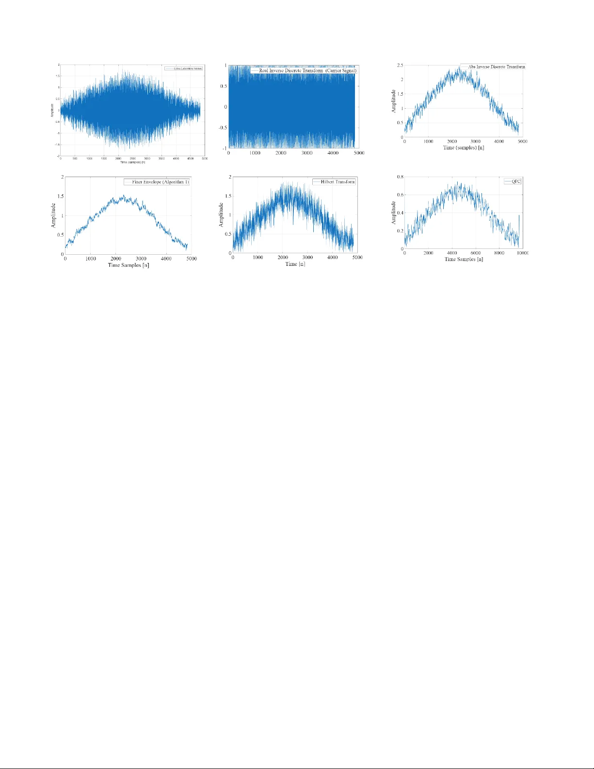
1 A New Perspective on Scale: A Novel T ransform for NMR Envelope Extraction Ehsun Assadi Abstract — Envelope extraction in nuclear magnetic resonance (NMR) is a fundamental step for processing the data space generated by th is technique. Envelope d etection accuracy improves with increasing the number of sampling points; however, we propose a novel transform that enables acceptable envelope extraction with significantly fewer sampling points, even without meeting the Nyquist rate. In this paper, we challenge the traditional scale definition and demonstrate that classic scaling lacks a physical referent in all situations. To achieve this aim, we introduce a scale based on the variations of space-invariant states, rather than the observable characteristics of matter and energy. According to this definition of the scale, we distinguished two kinds of observers: scale-variant and scale-invariant. We demonstrated that converting a scale-variant observer to a scale- invariant observer is equivalent to envelop extraction. To analyse and study the theories presented in the paper, we have designe d and implemented an Earth-field NMR setup and used real data generated by it to evaluate the performance of the proposed envelope-detection transform. We compared the output of the proposed transform with that of classic and state- of -the-art methods for parameter recovery of NMR signals. Index Terms — NMR, Spin-Echo, Time-Scale, Scale-Variant Observer, Scale-Invariant Observer, Envelope Extraction I. INTRODUCTION art h-f iel d nucl ea r magne tic res ona nce ( EF -NMR ) tec hni que util ize s the Eart h’s magnet ic fiel d as the mai n magn et ic fie ld, making it susce pti bl e to nois e. Enve lope ext rac ti on of no isy N MR spi n-ec ho s ign als is a fund ame nta l ste p in gene rat in g nucl ear magnetic reso nanc e image s. To ach ieve high er- fre quen cy est ima tio n precis i on and accurat e envelo pe det ect io n, a rela tive ly lon g meas ur eme nt time and a higher si gnal - to -no ise rati o (S NR) are re quir ed. In th is pape r, we int rod uce a nov el trans fo rm tha t uses more sa mpli ng points for spe ct ral analys is than the compan ion meth ods , maki ng it a powe rfu l tool for prec is e fre quen cy es ti mati on at low er fre quen cie s and ef fec tive e nvelo pe ext rac ti on. In thi s s tud y , we use Fr ee In ducti on Decay (FID) and spin- ech o NMR sig nals . FI D sig nals are trans ie nt res pons es from a spi n sys te m aft er an RF pulse ex cit ati on (see Fig. 1(a) ). Two suc ces si ve RF puls es produ ce a spin-e cho signa l . We design ed an Earth- fi eld Nuc le ar Magnet ic Res ona nce (N MR) sy ste m to obs erv e and study spin-ec ho signal s und er va ryi ng mag net ic field homog ene it ie s, which pave d th e wa y for the the oret ic al dis cus si on in the pa per (se e F ig. 2) . Corresponding a uthor: Ehsun Ass adi , (e -mail: ehsun. assadi@gmail.com) . (a) (b) Fig. 1. Different frames in NMR technolo gy. (a) Laboratory frame. (b) Rotating frame. Bri ef ly descri be the cha ra cte rist ic s of th e designe d NMR he re. A pol ari zer driver capabl e of deli ver ing 10A to gener ate a    pola ri zat io n fiel d is im ple ment ed a nd des igne d, a nd the RF tra ns mitt er and rec eive r coi ls are de si gne d for an 8 cm field of vie w, as show n in Fig. 2(a) . An RF trans mit te r cir cuit for gene rat in g a puls e se quen ce is impl eme nt ed and desi gne d (see Fi g. 2(b )). The scale si mul ator for sim ula tin g sc ale and fiel d shi mmi ng has b een des ign ed a nd i mpl eme nt ed, as s how n in Fig. 2(c) . A powe r ampli fi er with an over all volta ge gai n of   and fre quen cy bandw id th of 300 Hz is imple ment ed to ampl ify the mic rovo lt signa ls from the recei ver coil, as see n in Fig. 2(d) . Two FID and spin-echo signals generated by our setup and arising from a tube of wate r that is exposed to h igh f ield ho mogeneity and low field homog eneity a re shown in Fig. 3(b) an d ( e), respectively. These signals will be used to study the proposed transform's theo ry and, fin ally, to evaluate its per formance and that of o ther methods. The propos ed tr ans for m is appl ie d as envelope de tec tio n t o NMR s ig nals in this paper; the refor e, we r evi ew p revi ous st udie s on NMR signal envelope ext ract io n in the foll owi ng. Enve lope det ect io n via the Hilb ert tra nsfo rm has bee n widel y adopt ed in NMR and broad er si gna l proce ss ing appl icat io ns. Th e Hilber t tra ns form provid es an ana ly tic rep res en tati on of a real-va lued si gnal , from whic h the in st antane ous amplit ude (envel ope ) can be extrac te d. This tech niq ue is par ti cul ar ly effec ti ve in isola ting sl owl y varyi ng modul at io ns embed ded wi thi n osci ll ato ry sig nals . Re cen t work s h ighl ig ht th e evol ut ion of s urf ace NMR met hodo log ies from trad iti ona l time- doma in envel ope dete ction to frequ enc y-do mai n and st ead y-s ta te appr oac hes . Gromba cher et al. [1] int rodu ced a spectr al analys is (SA) envelop e det ectio n sc heme th at le ver ages di sc rete Fouri er tran sfo rms over s li ding win dow s of NM R data t o pr oduc e h igh- SNR e nvel ope s. Liu et al . [2] de vel ope d a comp reh ens iv e workfl ow for stead y- st ate f ree prec ess io n (SS FP) su rfa ce N MR da ta, introd ucin g met hods s uc h as tr ans ien t cull ing, pul se w ind owi ng, de -s piking , E 2 powe rl ine harm oni cs subt ra ction, and multi win dow spe ctr al ana lys is. The na rrow ban d col la pse a nd mult iwi ndow conc at ena ti on i mpr ove th e s tabi li ty of e nve lop e e xtr act ion . Alt hou gh t hes e me tho ds p resen t s tro ng co ntr ibu ti ons to N MR enve lop e extr act io n, they tr ade off envel ope conti nui ty and sa mpl e ric hnes s. A key li mita tio n of t hes e app roac hes is t hat the fin al envelo pe si gnal s ar e inh erent ly down-s amp led : by rel ying on sl idin g-wi ndo w disc rete Fouri er t rans form s cent er ed at spe ci fic fre que ncie s, the number of ext rac te d env el ope samp les is much fe wer than the origi nal tim e-dom ai n sig nal . This redu ct ion in sa mpl in g densi ty can limit tempo ral resol uti on and pote nt ial ly obscur e fine- scale varia ti ons in the envel ope , part ic ul arl y in early- tim e dat a whe re ac cur at e am plit ude t ra ckin g is cr iti cal . Tia n et al. [3] intr oduc ed a nove l app roac h tha t combine s third - orde r cumul ant s (TOC) with quadra ti c freque ncy co upl ing (QFC ) cons t rain ts to enha nce the ro bus tne ss of MRS si gna l ana lys is. T hei r method leve rage s the proper ty that high er-o rder cumu la nts suppre ss Gaus si an random noi se , whil e the QFC cons tr ai nt sel ect iv ely ret ain s freq uenc y comp one nts tha t sati sfy nonl ine ar coupl ing relat io nship s. The ir cont ri but ion provi des a comp le ment ar y pe rs pec tive by ad dres s ing noi se su ppre ss ion and para met er rec over y via nonl in ear fre quen cy-c oupl in g cons tr ai nts . The theore ti cal c ont ribu ti on of thi s ar ti cle lies i n i nt rodu cin g a new per spe cti ve on the fram es used in NMR technol ogy, which is shown in Fig. 1 . I n describing th e NMR tech nique, multiple reference frames are u sed to uniquely define physical quantities, such as the magnetic field and the angular momentum. Two main fram es that are constantly referred to in the NMR techniqu e, the laboratory frame and the rotating frame, are shown in Fig. 1(a) and (b), respectively. In the literature, the rotating frame is con sidered a frame o f reference that rotates with respect to the laborato ry fram e at a specific angular velocity , in both classical and quan tum views [4 ], [5]. In this paper, we introdu ce a new p erspective on scale that helps us redefin e the frames in Fig. 1 as o bservation s m ade by a unique observer, each from a d ifferent point of view . This novel perspective enables us to easily transfer betwe en t he laboratory and rotatin g frames, which correspond to the same envelope extraction. II. P ROBLEM D EFI NITION Regardless of the spectr al distributio n of a spin system, the maximum amplitude (at t = 0) of the FID signal depends on t he magnetic field strength and is reached at t = 0. The decay rate of an FID signal, known as the r elaxation time   , is r elated to the spectral distribu tion of magnetized spins  󰇛 󰇜 . The s pectral de nsity function 󰇛  󰇜 determines the characteristics of an FID signal in the laborato ry frame . If the receiver coil has a homogeneous reception field o ver the region of inter est, as is often as sumed, the FID signal r esulting fr om an  RF pulse takes the following f orm [5]:  󰇛  󰇜      󰇛  󰇜              (1) Suppose that the spectral d istribution of a spin system in the laboratory frame can be defined as a spectr al distribution with a fr equency shif t as   󰇛  󰇜  󰇛    󰇜 . Where   󰇛 󰇜 is the spectral distribu tion o f magnetized spin s in the labo ratory frame and 󰇛 󰇜 represents the spectral distribution o f magnetized spins in the rotating frame. The FID signal in the laboratory frame becomes:   󰇛  󰇜      󰇛󰇜              󰇟  󰇛  󰇜   󰇠             (2) The spec tral distribu tion of magnetized spins  󰇛 󰇜 is dependent o n the object's inher ent properties and is af fected by the main magnetic field inhomogeneity . When b oth the magnetic field and the sample that is exposed to the magnetic field ar e highly homogeneous, the FID signal exhibits a distinctive   decay; otherwise, it decays with a lower time constant n amed    . FID an d spin -echo signals of a tube of water exposed to higher and lo wer field homogen eity are shown in Fig. 3(b) and (e), respectively. The q uestion is, wh at if we con sider th e d ilation of an independent variable, such as time on a timescale, as th e leading cause o f the different decay rates of the FID signal in Fig. 3 (b) and ( e)? In o ther wo rds, we consider the d ilation or expansion of the time scale of f rames to be the cause o f the change in decay rate in the FID signal, rather than changes in spin energ y states resulting from d ifferent magnetic f ield hom ogeneities. (a) (b) (c) (d) Fig. 2. Earth-field NMR setup. (a) Polarizer, transmitter, and receiv er coils inside an electromag netic shield. (b) Transmitter and receiver RF board. (c) Scale simulator. (d) Power amp. 3 It is essential to define the time scale we intend to use in this paper precisely . The time- scale used in the paper h as four main properties: • First, the uniform motion is a rectilinear motion that is shaped by the motion of a free particle that includes at least three states (not necessarily distinct) of energy during the motion of the free particle . • Second, the motion of a free p article is unifor m on the time scale. • Third , equal intervals of time are those in which a free particle travels eq ual distances. • Fourth, the least interval o f time is determin ed by the observer , not the motion of the free particle . We must determine whether the time dilation of the synthesized signals in th e laborator y fram e (Fig. 3(a)), leading to Fig. 3(d), co rresponds to the p hysical observation s shown in Fig. 3(b) and Fig. 3(e) within the introduced time scale. According to the pr operties of th e time -scale defined above, when the carrier signal (     󰇜 experiences time-scale scalin g, the envelope should exhibit the same kind of scaling. The argumen t of the carrier sign al is linear in time; hence, the envelope's ar gument should be lin ear in time as wel l . T he on ly way to satisfy this is that the field distribution inhom ogeneity (        ) should lead to a L orentzian distribution as follows:  󰇛  󰇜      󰇛    󰇛    󰇜  󰇜 (3) Assuming that the magnetic f ield inhomogeneity with Lorentzian distributio n is time-invar iant, the FID signal in the rotating frame becomes:   󰇛  󰇜                       (4)   󰇛  󰇜         󰇛      󰇜 (5) Where   is the thermal equilibrium value for the bulk magnetization at t=0 in the p resence of   ,   is the Larmor precession angular f requency,   is the tran sverse relaxation time, and  is the angle between the coil's axis and the external magnetic field. The energy diff erence b etween the adjacent spin states due to the extern al magn etic field strength B0, an d the total number of spins at room temper ature, are considered to remain con stant over tim e-scale changes. In Fig. 3(a) and (c), we generated two sy nthetic NMR signals in laboratory and ro tating frames, respectively, u sing Eq. (4) - (5) . By increasing   in Eq. (4), we simulate the NM R signal exposed to lower-field homogeneity, as shown in Fig. 3(e), and present the results in Fig. 3(d) and 3 (f). Overall, the field homogeneity in both synthetic an d real sign als leads to a Lorentzian distribu tion. Time-scale scaling is not directly supported in discrete- time systems, as th ey h ave a fixed sampling frequen cy. Thus, time scaling in discrete -time consists of two parts: down -samp ling the signal and shif ting the remaining sample points to the scaled time scale with equal intervals but smaller inter vals. In discrete- time , downsampling does not change the signal's frequency content; howev er, the time interval is stretched . To keep the (a) (b) (c) (d) (e) (f) Fig. 3. Effect of time -scale scaling on differen t frames. (a) Synthesized signal in the labo ratory frame. (b) F ID and spin-echo signal of a tube of water ex posed to a high field h omogeneity. ( c) Syn thesized envelope sign al in the rotating fr ame. (d) Synthesized signal in th e laboratory frame. (e) F ID and spin -echo sign al of a tu be of water ex posed to a low f ield homogeneity. (f) Synthesized envelope signal in the ro tating frame.   Eq. (6) & Eq. (7) Decreasing fie ld homogeneity Eq. (6) & Eq. (7)   4 sampling frequency f ixed during do wnsampling in the discrete domain , we shift the down sampled samples to the left. First, we zero-pad the or iginal signal by a factor of M ; second, downsample the zero-padded signal as follows:      󰇟  󰇠                (6)  󰇟  󰇠    󰇣   󰇤         (7) Where,  is sam pling po ints, and  is the downsam pling factor. After compressing the signal using Eq. ( 7), we use interpolation t o ge nerate new s amples with non-integer indices. The above time-scale shrin kage does not violate the optimal sampling pattern for measuring the NM R spin -spin relaxation time [6 ]. The results o f such time scaling in discrete- time do n ot have a physical referent , se e Fig. 3. The time-scale transform results for the rotating fram e in Fig. 3( f ) are co nsistent with the physical o bservation of d ecreasing field h omogeneity , as shown in Fig. 1(e), while the scaled results for the laboratory fr ame in Fig. 3(d) did not ma tch with the physical observation of decreasing field homogeneity , as shown in Fig. 1 (e) . Sin ce the frequency o f the signal is changed in Fig. 3(c), while the frequency of signals with two different field homogeneit ies in the real exp eriments is the same , as shown in Fig. 3(b) and (e). In continuous time, the m athematical transfo rm we u sed for time scaling was the Galilean transfor m, which preserves the laws of electromagnet ic fields. Besides, fram es are mathematical metric spaces that remain metrics during the transform . It seems the prob lem is related to the scale at which two observers, one in the laboratory and one in a rotating frame, experience it . We try to define a unified scale for both observers in the frames. To solve the problem, we introdu ce the scale for time-scaling b ased on the observer ’s proper ties rather th an observable characteristics of matter and energy. First, we need to define the observer we use in the paper. We confine the observer to some constrain ts fo r co nsidering scaling in time as an inv ariant variable to acco unt for the variation of    . This appro ach en ables us to find a p hysical referent fo r the time scaling in the discrete time we used above. For hav ing a physical referent for such mathematical time -scaling in a discrete domain , we may confine the o bserver to three ru les: • First, the observer should have the same fr equency sampling rate in all frames we study. • Second, the obser ver’s ob servation is time -invarian t in all frames. • Third, the o bserver mu st observe at least thr ee samples, in wh ich two of them must be related to distinct states or two different lev els of energy. This enables us to define smaller quantized steps, which a re required by the fourth property of th e time-scale. Based on the first property of th e time-scale and the third property of the observer, no ob server o bserves a mass in the time-scale that travels with a constant speed without ch anging the amount of mass or en ergy. This property helps us overcome the classic scale problem, as seen in Fig. 3. To observ e such a constant-v elocity mass, the observer should sample the rising and falling times of the mass's motion . A mass with a higher speed will have a sharp er rising and falling time than a mass with a slower speed. The observer who observes the higher speed mass should have a higher sampling frequency to be ab le observe such a sh arper edge, b ut this v iolates the firs t pr operty of the observer. To maintain the same sampling frequency for both observers, the times of th e two observ ers will differ . In this paper, we inten d to u se a unique observer with varying points of view; in other words, the observers observe the same mass in the same ener gy states from different points of view. Based on the above d iscussion, th e frames in Fig. 1 are not frames ; in stead, they are observatio ns by the same observer with two differen t points of view on the state of en ergy being observed . The diff erent points of view in th is pap er relate to scale, which we will explain in the following sectio n . Contrary to the frame concept, which holds that different observers with varying sampling fr equencies observ e masses at diff erent speeds or in different energy states, our concept h olds that observers observe the same mass at the same energy level fr om two diff erent poin ts of view, with a constant sampling frequency . Theref ore, we suggest that rea ders ch ange the word frame in this paper to a point of view to achieve a more precise understand ing o f the concept the pap er aims to introduce. By following these rules for observers, the o bserver should sample the signals at the sam e freq uency. Now, we define the scale we u sed in the paper . Variation in space-invar iant states, such as spin , is considered a scale rather than a change in physical size, space, or time intervals. In ot her words, the frequency o f the space -inv ariant state variation s is regarded as a scale in the paper. Acc ording to our definition of the scale, there are two types o f observers: scale-variant and scale-invarian t, bo th o f which meet th e thr ee o bserver properties we introduced. The difference between a scale-variant and scale-invariant observer is based on their knowledg e about either the physical scale or the state of the phenomenon being observed. The observer who observes at least two d ifferent space -in variant states of the object out of three samp les with varying intervals of time is called a scale-var iant observer. Moreover, there are two types of scale -variant observers: on e that observes states continuou sly and the other that observes them discretely or q uantitatively. To avoid burdening the paper, we av oid introducin g these two types of scaled observers; instead, we introduce an equivalence principle. W e need to introduce an eq uivalence relation between scale- variant and scale-invarian t ob servers to relate two fram es fro m different points of view. We will use this eq uivalence in the proposed transform . A scale-invariant o bserver is eq uivalent to the discrete scale- variant o bserver that o bserves only a unique state. One of the physical proper ties to distinguish between a scale- invariant ob server and a scale -var iant observer is the relation between energy and the frequency of changing the states. The coefficient   󰇛    󰇜 is only constant fo r a scale -invariant observer during the classic sca ling procedure. T he scale-variant observer will co nsider th at the energy and, consequently, the mass of the ob ject is changed when the scale , in its classic definition , of the time-scale ch anges. I f mathematically scaling 5 the time -scale , as described as down -sampling and shifting in Eq. (6) -(7), one wan ts to h ave a physical referent,    should remain constant during the sca ling only for those observers that are free of scale, in its new definition, but have the s ame sampling frequency in a metric space . Ho wever,    cannot remain con stant for a scale-variant o bserver who con siders the same object to hav e lower energy or lower mass at different scales applied to th e time scale. For in stance, the constan t    i s fixed by changing field homogeneity in our experiments, as shown in Fig. 3(b) and (e). However, it changes through the classic time-scale scaling (downsamp ling and shifting process) in the laboratory frame in Fig. 3(b) a nd ( d). The spin en ergy, powered b y th e Earth' s magnetic field, and the L armor frequen cy in high - an d low -field homogeneities are the s ame in Fig. 3(b) an d (d), respectively. It means that    r emains constant in both cases; h owever, the Larmor frequen cy changes with time scaling in Fig. 3(a) and (d), which means the spin s' energy sh ould decrease due to time dilation. To get back to our main problem, considering the homogeneity effect as a time -scaling ef fect, we hav e to chan ge the scale-variant observation, a laboratory view (see Fig. 1 (a)), to a scale- invariant observation as a r otating frame (see Fig. 1 (b)), while both observations experience the same energy. In the following, we introduce a no vel transfo rm that conv erts the scale-variant o bserver into a scale-invariant ob server. III. P ROPOSED T RAN SFORM In this section , we introduce the proposed transform that converts scale-variant observations into scale -invariant ones . According to the eq uivalence, a scale-invariant o bserver must observe a unique state out of many states. Additionally , the observer must observe at least three samp les, which include at least two distinct states; o therwise, based on the introduced time-scale p roperties, changing the energy state o f a body will not be distinguishable from a free particle with uniform motion that is scaled in space over time. On e o f those three samp les can depend on the o ther two, but each of the two samp les sh ould relate to two distinct states. To have such an ob server, the observer should o bserve samples in both the present and the future simultaneously. To this en d, th e signal should be transformed into a complex signal, known as the analytic sign al, in which time must be treated as an invariant v ariable. Traditional classical appro ach es to represen ting and analyzing sign als includ e integral transforms such as the Fourier, Laplace, and Hilb ert transforms . The Hilbert transform is a clas sical app roach for converting real signals into analytic signals. Th e Hilbert transform of a signal is def ined as the signal in which all freq uency components o f the o riginal sig nal have their phase shifted by 90°. The shifted signal can be interpret ed as the signal in th e future [7], [8]. The analytic signal is the signal in quadratu re with the original signal; when add ed to the original signal, the oscillating signal beco mes a ro tating vector. As shown in Fig . 4, an analytic signal is represen ted by a phasor rotating in the complex plane. In this paper, we discuss the discrete co mplex space. A ph asor can be viewed as a vector at the origin of the co mplex plane , having a length A(t) and an angle, or an angular position (displacement) 󰇛 󰇜 [ 9]. As discussed, the introduced scale is independent of mass for a scale-inv ariant o bserver. Thus, to change a scale-v ariant observer to a scale-inv ariant observ er, we need a variable that is independent of mass and energy, and a metric that is a constant, b ut infinitely divisible quan tity. In the complex plane representation , length 󰇛  󰇜 an d the least spatial interval  󰇛 󰇜 of the Hilb ert transform is proportional to mass; therefo re, the multiplication of any scale of 󰇛 󰇜 depends on mass and energy. In comp lex coord inates, th e length  󰇛󰇜 is related to mass; however, the least spatial interval in the complex plane is the instantan eous phase  󰇛 󰇜 wh ich is independen t of mass . Moreover, as shown in Fig. 4, it is a constant metric that can be discretized an infinite numb er of tim es. Hence ,  is th e third observation gen erated by the two other samples in th e real and imaginary coordinate systems, wh ich satisfy the third ru le defined for th e observation. The instant freq uency  󰇛󰇜 measu res the rate and d irection of a phasor rotation in the complex plane. Th e i nstantaneous frequency of the red sig nal in Fig. 4 fo r a scale -invar iant observer is th e same central angu lar frequency   and only th e length  󰇛 󰇜 chan ges by time; thus, the mean valu e of the instantaneous frequen cy is the same as the central frequency   . Thu s,         and     , where   is the average angular speed. The least spatial interval instantaneous phase in discrete form can be obtained as follows [9]:                     (8)       (9) Assuming that the least interval  is th e sampling rate in the discrete f orm, yield ing the final coefficien t        . In the proposed tran sform, we call   transfer frequ ency. As discussed ,  is a variable indep endent of mass, and a basis generated from it will d istinguish rec tilinear motion from rotation and acceleration, removing the scale dependence o f the scale-variant o bserver. Fig. 4. Signal expression in complex domain (the figure inspired by [9]). 6 The desired an alytic signal wil l b e generated by th e b asis that contains the abov e co efficient, su ch th at       . Thus, we multiply this coefficient by all the sin e and cosine basis of t he Fourier transform. The p roposed meth od in contin uous fo rm for a synthetized FID signal is given by : Forward continuous tr ansform:  󰇛   󰇜    󰇛   󰇜                   󰇛        󰇜 󰇛        󰇜   󰇛       󰇜  ( 10 ) Inverse continuous Transfo rm:   󰇛  󰇜                           󰇛         󰇜        ( 11 ) The p roposed meth od in discrete form for a finite signal with finite samples can be expressed as: Forward discrete transform:  󰇟  󰇠    󰇟  󰇠               󰇟   󰇠 ( 12 ) Inverse discrete transform:  󰇟  󰇠       󰇟  󰇠             󰇟     󰇠 ( 13 )      󰇟 󰇠  ( 14 ) Where,   and   are tran sfer and samplin g frequencies, respectively. Also, N is the to tal number of samples . The resu lts of applying the forward an d inv erse continuous transforms to the FID sign al in Fig. 1(a) are shown in Fig. 5. The co ntinuous form in Eq. (10) corresponds to the classic time- domain scalin g, resulting in scale- variant observatio ns. Its output is the scaled version of the original signal, which lacks a physical referent, as d iscussed in Section I I and shown in Fig. 3. In addition, the continuous i nverse form does not produce an analytic, complex signal. The reason is that  , which is considered the inv erse of the sample rate, does not hold in continuous form. Because of its infinite frequencies, it does not have a constant sampling frequency throughout the transform, violating the second rule of the observer. The discrete fo rm with a fixed nu mber of samples will solve th e pro blem. The in verse transform of the discrete form generates an analytic signal whose absolute value will change the scale -variant obser vation to a scale-invariant observation. The o utput of Eq. (13) is an analytic signal that consists of real and imag inary parts. The absolute v alue of the analytic signal in Eq. ( 14) resu lts in an envelope signal. The results of applying the forward and the inverse discrete transform on the FID signal in Fig. 1(a) are shown in Fig. 6. Thanks to the complex s ignal generated by the inverse of the proposed transform , its main a dvantage is that adherence to the Nyquist rate is unnec essary; it suffices for the nu mber of samples to equal the transfer fr equenc y (   ) . In other words, w e can violate the Nyquist rate in the p roposed method, which can be reduced to th e transform's tran sfer fr equency, and the sampling fr equency an d number of samples can be red uced according ly. IV. R ESULTS A. D -delayed Pulse Stu dy To better understan d the power of the proposed method for frequency estimatio n precision, we stud y the rectang ular pulse function, see Fig. 7. Three situations for pulse study are considered: a pulse with D -delay in Fig . 7(a) , a pulse with 2D - delay in Fig. 7(b), and a pulse with D-d elay while the transfer frequency in Eq. (12) is double of the transfer frequen cy used for the former p ulses. All pulses have a fixed p ulse width and are samp led with the same sampling frequency equal to    . (a) (b) (c) (d) Fig. 5. Proposed Tr ansform in continuous form. (a) continuou s transform. (b) Abs of inverse continu ous transform. Fig. 6 . Pro posed Transform in Discrete form . (a) Discrete transform. (b) Abs of inverse discrete tran sform. 7 As sh own in Fig. 7 (d)- (f), the proposed transform pr ovides a zoomed and precise frequency estimate . The ab solute value of the real part of the proposed transform, Eq. (12), is shown in a blue dash ed line, r epresenting the en velope of th e fringes generated by the absolute value of t he real and imaginary parts. Thanks to the fringes gener ated by th e absolute val ue o f the real and imaginary par ts of Eq. (1 2), the original signals can be easily recon structed u sing the equation below :               ( 15 ) Where   is a constant,   is the distance between fringes, d is the delay measured in samples (    is the delay in seconds ) ,   is the transfer frequency,   is frequency sampling, and N is the number of sample p oints. Since    d oes not c hange for a scale- invariant observ er, it guar antees that   is a constant. The fringes can help to recover the delay an d transfer frequency used in the proposed transf orm. In addition, the pulse analysis allows us to und erstand how transfer frequency and delay affect the precision of frequency estimation. As shown in Fig. 7, the study of a rectan gular pulse signal in dicates that th e transfer frequency should be smaller to achieve a higher frequency estimate. Mo reover, the signal should be d elayed to obtain even more fring es wi thin the envelo pe, leading to a higher -frequency estimation. On the other hand, a lower transfer frequency eliminates high frequencies, so the reconstructed rectangular pulse canno t be well reconstructed . If we consider signals as the s um of a DC component and the original signal, the DC component will represent the pulse signal and will not be reconstructed well. Hen ce, we need to remove the signal mean before using the proposed tran sform for better en velope extraction, and in troducing a delay will lead to higher -frequency estimation and improved signal reconstruction . Thus, we introduce som e d elays into the FID signals and rem ove the signal mean in the experiments. Although the DC co mponent of the signal will be removed, the residual sign al will still contain a rectan gular push. Therefore, we first extract the env elope from the a bsolute value of the outp ut of Eq. (1 4), th en ex tract the carrier signal . Then , we extract the ca rrier envelope usin g Eq. (13) and sub tract it from the original envelope, leading to a fin er envelope extraction, as will be seen in the following subsection . B. Synthetic Data Study A synthetized noisy FID s ignal was co nstructed based on Eq. (4) with a Lamor frequency of 5 Hz, amplitude 10V , relaxation time (    ) 2    , and the initial phase 0. The s ignal was sampled at a fr equency of 100 Hz with a samp ling interval   =(1/f s ) = 0.01 s, resulting in 1885 data points over a time period of   . I n NMR signal processing, the observ ed signal is typically corrupted by a combination of differen t noise s ources. T he most common types in clude Rician-d istributed noise, Gaussian (white) noise, Joh nson (therm al) noise due to heat generation in the device's magnetic cores, and harmonic interference from the power line. To model an ideal n oisy s ignal, we consid er a mixture of these noise components with th e fo llowing characteristics: Rician-d istributed noise is simu lated b y adding random samples dr awn from a noncen tral chi distribu tion with a noncentrality parameter o f 1 , a scale param eter of 0.3 , with approximately zero mean and amplitude of   , Gaussian (a) (b) (c) (d) (e) (f) Fig. 7. Apply ing th e propo sed transfo rm in discrete f orm on a pulse function with a fixed pu lse width . (a) Pulse f unction with D - delay. (b) The p roposed forward discrete transfo rm of ( a) with the transfer function   . (c) Pulse function with 2 D-d elay. ( d) The proposed forward discrete transform of (c) with the transfer fun ction   . (e) Pulse function with D-d elay. (f) T he proposed fo rward discrete transfor m of (a) with th e transfer functio n   . 8 random no ise with zero mean an d a stand ard deviation o f    and amplitude of  , Jo hnson noise calculated for the highest temperature of the coil s measured at the lab , which was   , and harmonic interferen ce simulated as a sinusoidal disturbance at    with amplitude  . The constructed FID signal is shown in Fig. 8(a). As d iscussed, there is no need to adhere to the Nyquist rate and the number of samples equal to th e transfer fr equency (   ) is su fficient in the proposed transform . Fo r this reason , we preprocess the orig inal signal by downsampling it by a fac tor of 8 to be processed by the proposed transfor m and by the Hi lbert transform; however, in other meth ods, in man y cases, due to the use of Fourier transfo rms or LTI filters , it is n ecessary to m eet the Ny quist rate. For example, in the QFC meth od, b ecause band-pass f ilters are used , the Nyq uist rate must be satisfied . This is the reason for the difference in the number of samples observed in Fig . 8. (c)- (f) . Despite the different number of samples, the time is the same in all of them. The p roposed transform produces a fin er envelop e in Fig. 8(c) than the Hilb ert transform and QFC metho ds, as seen in Fig. 8 (e) and (f), resp ectively. In addition, the extracted envelope gets finer with rep rocessing by th e proposed transform , as shown in Fig. 8(d). C. Real NMR Data S tudy The rea l FID and spin- echo signals used in this paper are obtained v ia the setup sho wn in Fig. 2. The Earth's magnetic field was measured in th e laborato ry to be      with a magnetom eter , whose Larmor frequency was calculated to be 1692 Hz. The polarization of the mag netic field   is    . We used a sinu soidal RF pulse with a rec tangular push with   RF pu lse duration . The acqu isition time is set to 5s for the water sample. We did not u se any averaging operation of the oscilloscope to acquire the NMR signals. The spin-echo signal from a tube of wate r exposed to h igh - field homogeneity, sh own in Fig. 3(b), is cropped and processed. The extracted envelope of t he proposed transform is compared with those of the class ic Hilber t tran sform and the QFC method. As shown in Fig. 9, the proposed transform extracts a finer envelope than the o ther methods; moreover, it analyzes a larger number of samples because it does not require meeting th e Nyquist rate. V. C ONCLUSI ON We challenged the classic def inition of scale , which primarily r elies on physical properties of objects. We defined scale based on variations in space -invariant states, rather than on observable character istics of matter and energy. According to the new perspectiv e on scale, we con fined the observer to three p roperties an d catego rized ob servers into two types: scale- variant and scale-invariant. These prop erties help to confine the frames to unique observers. Then, we introdu ced a n ovel transform that converts a scale-variant ob server into a scale- invariant ob server. We showed that the envelope of the NMR signal in the laboratory frame is scale-variant, whereas the signal in the rotating frame is scale -in variant. The introduced transform g enerates an analytic signal wh ose absolute value yields the envelo pe of the NMR signal, and this observatio n is scale-invarian t. In addition, the advan tage of the proposed transform is that it do es not require meeting the Nyquist rate. The transform outp erforms th e classic and state- of -th e-art methods for NMR signal env elope extraction. R EFERENCES [1] D. Grombacher , L. Liu, M. A. Kass, G. Osterman, G. Fiandaca, E. Au ken, and J. J. Larsen, “Inver ting surface NMR (a) (b) (c) (d) (e) (f) Fig. 8 . Applying the pro posed tran sform in d iscrete form on a synth esized NMR FID signal . (a) A synthesized NM R FID signal . (b) The extracted carrier of (a) using the inverse discrete transform . (c) The extrac ted envelope of (a) u sing the inverse discrete transform . (d) Applying the proposed inverse discrete transform on ( c). (e) Extracted envelo pe by the Hilbert tran sform . (f) Extracted envelo pe using the QFC [3] . 9 free induction decay data in a voltage - time data s pace,” Journal of Applied Geophysics, vol. 172, p . 103869, Nov. 2020. [2] L. Liu, D. Grom bacher, M. P. Griffiths, M. Ø. Vang, an d J. J. Lar sen, “Signal pr ocessing stead y - state surface NMR data,” IEEE Tr ansactions on Instrumentation and Measurement, vol. 72, pp. 1 – 13, 2023. [3] L. Tian, Y. Zhang, H. Wan g, Q. Chen, and M. Li, “Th ird - order cumulan ts with quadratic f requency coupling constraints for robust MRS signal analysis,” IEEE Transactions on Biomedical En gineering, vol. 7 2, no. 4, pp. 1023 – 1035, Apr. 2025. [4] A. Abrag am, *The Prin ciples of Nuclear Magn etism*. Oxford, U.K.: Ox ford Univ. Press, 196 1. [5] Z .-P. L iang and P. C. Lauterbur, *Principles of Mag netic Resonance Im aging: A Signal Processing Perspective*. N ew York, NY, USA: I EEE Press/Wiley, 200 0. [6] P. L. Carson, H. N. Yeung, M. O’Donnell, and Y. Zh ang, “Optimal sampling strategies for the measurement of spi n – spin relaxation times,” Med. Phys., vol. 15, no. 5, pp. 767 – 775, Sep. – Oct. 1 988. [7] M. A. Khan and S. A. Malik, “Real - time FPGA implementation of a 90° phase shifter based on Hilbert transform,” IEEE Access, vol. 1 2, pp. 117345 – 117356, Oct. 2024. [8] Gabor, Dennis. "Theory of communication. Part 1: T he analysis of information." Journal of the Institution of Electrical Engineers-p art III: radio a nd communication engineering 93, no. 26 (1946): 4 29-441. [9] M. Feld man, “Hilbert transform in vibration analy sis,” Mechanical Systems and Signal Processing , vol. 25 , no. 3, pp. 735 – 802, Apr. 2011. doi: 10 .1016/j.ymssp.2010.07.018 (a) (b) (c) (d) (e) (f) Fig. 9. Applying the proposed transfo rm in discrete form on a real NMR spin-ec ho sig nal. (a) NMR spin -echo signal o f a tu be of water. (b) The extracted carrier of (a) using the inverse discrete transfor m . (c) The extracted envelope of (a) u sing the inver se discrete tran sform. (d) Ap plying the proposed inverse discrete transfo rm on (c). (e) Extracted en velope by the Hilb ert transform . (f) Extracted envelope u sing the QFC [3] .