Structured Analytic Mappings for Point Set Registration

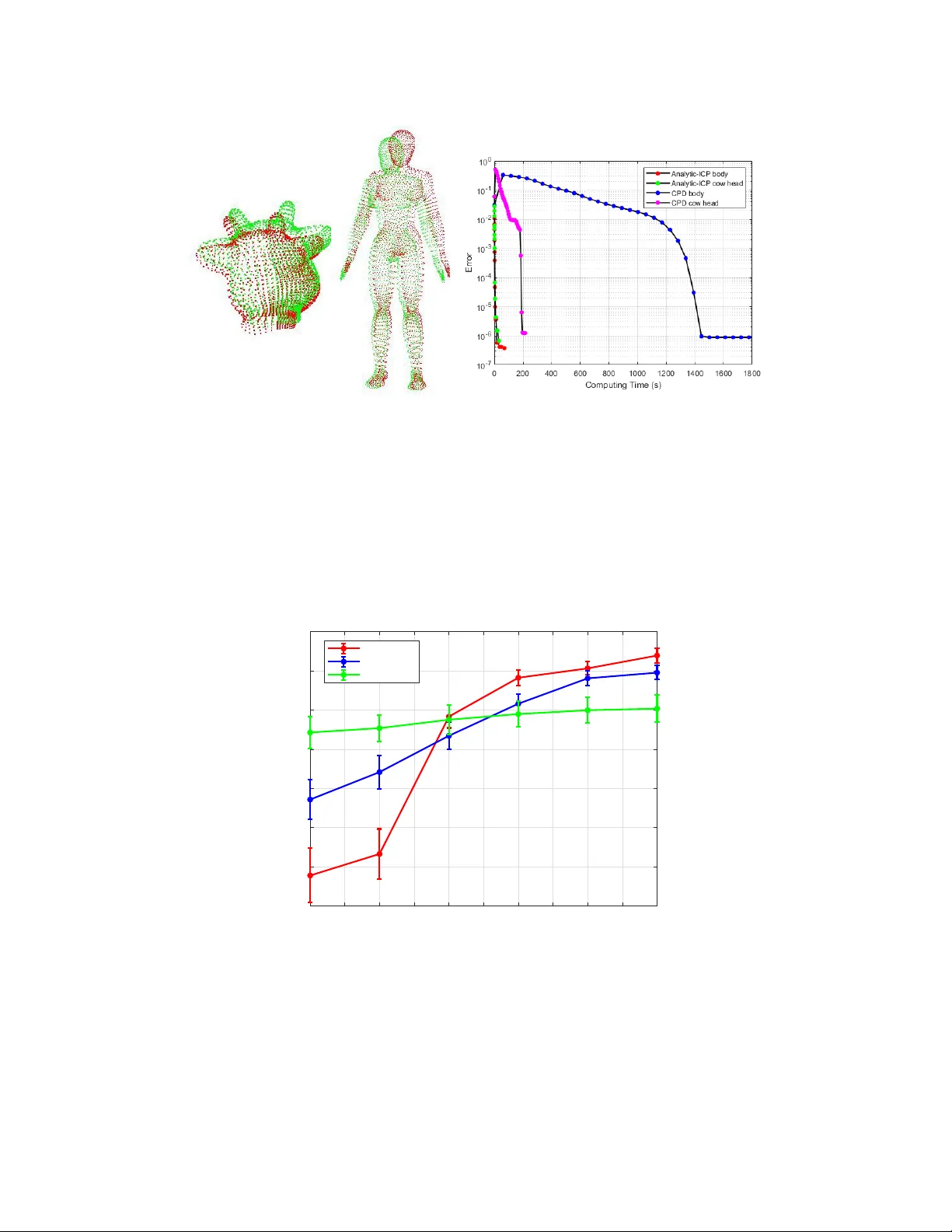
STR UCTURED ANAL YTIC MAPPINGS F OR POINT SET REGISTRA TION ∗ WEI FENG † , TENGDA WEI ‡ , AND HAIYONG ZHENG † § Abstract. W e present an analytic approximation model for non-rigid point set registration, grounded in the multiv ariate T aylor expansion of v ector-v alued functions. By exploiting the algebraic structure of T aylor expansions, we construct a struc- tured function space spanned b y truncated basis terms, allowing smooth deformations to b e represen ted with lo w complexit y and explicit form. T o estimate mappings within this space, we dev elop a quasi-Newton optimization algorithm that progres- sively lifts the iden tity map in to higher-order analytic forms. This structured framework uniﬁes rigid, aﬃne, and nonlinear deformations under a single closed-form form ulation, without relying on k ernel functions or high-dimensional parameterizations. The prop osed mo del is embedded into a standard ICP lo op—using (by default) nearest-neighbor corresp ondences—resulting in Analytic-ICP , an eﬃcient registration algorithm with quasi-linear time complexit y . Experiments on 2D and 3D datasets demon- strate that Analytic-ICP achiev es higher accuracy and faster conv ergence than classical metho ds such as CPD and TPS-RPM, particularly for small and smo oth deformations. Key w ords. Structured T a ylor expansion, Analytic appro ximation, V ector-v alued functions, Poin t Set registration, Non- Rigid registration, ICP F ramework 1. In tro duction. P oint set registration is a fundamen tal problem in computer vision and geometric data analysis, with wide-ranging applications in 3D reconstruction [28], sensor alignmen t [11], motion track- ing [10], and robotic perception [36]. While rigid and aﬃne methods ha v e been extensiv ely studied [4, 42, 48], registering p oint sets under smo oth non-rigid deformations remains a signiﬁcan t challenge due to the need for expressive mappings in high-dimensional spaces. Suc h techniques are crucial in mo dern systems ranging from visual metrology [28] to augmented realit y [50] and autonomous navigation [14]. Most existing non-rigid registration methods adopt non-parametric models, such as radial basis func- tions [17], Gaussian mixtures [33], or statistical estimation frameworks [25, 19]. While ﬂexible, these mo dels t ypically require large num b ers of basis functions or parameters to express complex deformations, result- ing in high computational complexity and increased risk of o v erﬁtting [31, 35, 43]. T o ensure n umerical stabilit y , additional regularization is often introduced, which ma y obscure geometric structure and hinder in terpretability . F rom a mathematical p ersp ective, m ultiv ariate T aylor expansions oﬀer a classical framework for ap- pro ximating smooth functions via structured p olynomial bases. In particular, V etter’s w ork [45] provides a general formulation for matrix- and v ector-v alued T aylor expansions, enabling analytic mappings to be expressed with controllable complexity and explicit algebraic structure. Despite its theoretical app eal, this form ulation remains underexplored in computer vision and registration tasks. In this paper, w e presen t the ﬁrst application of m ultiv ariate T a ylor expansion of v ector-v alued functions to non-rigid p oint set registration. By constructing a low-dimensional admissible function space spanned b y truncated T a ylor basis terms, we pro vide a compact and expressiv e framework capable of representing smo oth deformations without relying on kernel-based mo dels or dense parameter sets. T o illustrate the expressiv e capacity of low-order analytic expansions, we show in Fig. 1 a series of 2D deformations generated from a second-order T a ylor model with only three parameters. Despite its simplicit y , the mo del can pro duce a rich v ariety of nonlinear and smo oth transformations. Based on this represen tation, we design a progressive ﬁtting algorithm that lifts the identit y map to higher-order analytic forms via structured quasi-Newton optimization. This metho d is integrated into a standard ICP lo op—with (b y default) nearest-neighbor corresp ondences—to construct Analytic-ICP , a fast and robust registration algorithm that supp orts hierarc hical reﬁnemen t of rigid, aﬃne, and nonlinear map- pings. Our main con tributions are summarized as follo ws: • W e presen t the ﬁrst structured appro ximation framew ork based on m ultiv ariate T aylor expansions of v ector-v alued functions in computer vision. This formulation enables interpretable and hierarchical mo deling of smo oth deformations, and pro vides a principled foundation for registration and beyond. ∗ Submitted to the editors DA TE. † College of Electronic Engineering, Ocean Universit y of China, Qingdao 266404, China (weifeng@stu.ouc.edu.cn, zhenghaiy- ong@ouc.edu.cn). ‡ School of Mathematics and Statistics, Shandong Normal Univ ersity , Ji’nan 250014, China (tdwei123@sdnu.edu.cn). § Corresponding author. 1 2 WEI FENG, TENGD A WEI, AND HAIYONG ZHENG Analytic mapping:  x 1 x 2  =  0 0  +  1 a 1 0 1   y 1 y 2  + 1 2!  a 2 0 0 0 a 3 0    y 2 1 2 y 1 y 2 y 2 2   Eﬀect of parameter ( a 1 , a 2 , a 3 ) p erturbation in 2D second-order T aylor expansion. (0, 0, 0) (0.5, 0, 0) (0, 0.9, 0) (0, 0, 0.7) (-0.5, -1.2, 0) (0, 0.9, -0.5) (0.5, 0, -0.7) (-0.2, 1.2, 0.8) Fig. 1: Illustrative eﬀect of second-order analytic deformation. Ev en with only three tunable coef- ﬁcien ts ( a 1 , a 2 , a 3 ), the second-order T aylor expansion mo del produces a div erse range of smo oth, nonlinear transformations. • W e formalize a matrix–vector representation of analytic mappings using gener alize d derivative ma- tric es and gener alize d monomial ve ctors , and pro ve a Structured Appro ximation Theorem establishing the approximation capabilit y of truncated T aylor mo dels o v er smo oth mappings. • W e construct a low-dimensional function space spanned by truncated T aylor basis terms, unifying rigid, aﬃne, and nonlinear transformations within a single closed-form expression. • W e design a progressive quasi-Newton ﬁtting algorithm that incremen tally lifts the iden tit y map in to higher-order approximan ts, oﬀering con trollable model complexity and eﬃcient conv ergence. • W e integrate the prop osed framework into an ICP-st yle optimization routine. The resulting Analytic- ICP algorithm achiev es quasi-linear complexit y and outp erforms classical non-rigid metho ds (e.g., CPD, TPS-RPM) in b oth accuracy and eﬃciency on 2D and 3D registration tasks. T o facilitate repro ducibility , source co de and data are av ailable; see Section 7.1 for details. 2. Related W ork. W e prop ose a no vel analytic mapping mo del that can b e in tegrated into many unsup ervised registration frameworks to impro ve their performance. In this section, w e brieﬂy review the dev elopment of rigid, aﬃne, and non-rigid registration techniques that are relev an t to our metho d. 2.1. Rigid and Aﬃne Registration. The Iterativ e Closest Poin t (ICP) algorithm [17] is one of the most fundamen tal and widely used geometric registration metho ds. It alternates b et ween estimating corresp ondences and ﬁtting orthogonal transformations. Due to its simplicity and eﬃciency , ICP has b ecome the de facto standard for rigid registration in industrial applications [32, 47], and has inspired n umerous v ariants [42, 52, 40, 29, 30, 48, 7]. Aﬃne registration [41, 20, 23, 12] extends the rigid mo del by allowing linear deformations. It preserves the simplicity of parameterization and do es not require additional constraints, making it highly practical. The num ber of parameters inv olv ed is only the square of that in rigid registration. 2.2. Non-Rigid Registration and Statistical F rameworks. The Non-Rigid ICP (N-ICP) [6] was among the ﬁrst to extend the ICP framework to non-rigid settings b y mo deling aﬃne transformations ov er smo oth manifolds. Ho w ev er, its computational complexit y is signiﬁcan tly higher than rigid ICP , whic h limits STRUCTURED ANAL YTIC MAPPINGS 3 its practical use. Diﬀeren tial geometry-based metho ds [38, 1, 13, 51, 49, 21] ha v e made considerable progress b y lev eraging in trinsic surface properties and geometric feature spaces. While these methods ac hieve high robustness and accuracy , they typically rely on 3D reconstruction and are challenging to implemen t in real-w orld applications. In practice, registration algorithms based on one-to-one corresp ondences, suc h as ICP , are highly eﬃcien t. Ho wev er, due to the non-conv exity of the mapping supp ort and the lac k of closedness in the mapping space [46], such metho ds struggle to ac hieve optimal solutions in non-rigid scenarios. T o address these issues, a large class of softassign-based metho ds has b een developed. Notably , the RPM [17] and EM [9] framew orks relax the hard correspondence constrain t and in troduce probabilistic mo dels to improv e conv ergence. By using Gaussian Mixture Mo dels (GMM), these approac hes reframe p oin t set registration as a statistical estimation problem [8]. The TPS-RPM algorithm [17] combines the robustness of the TPS mo del [5] with the annealing strategy of RPM. It is particularly eﬀective for handling noise and outliers in 2D and 3D data, but does not generalize w ell to higher-dimensional or more structured deformation problems. The Coherent Poin t Drift (CPD) algorithm [34, 33] builds up on Motion Coherence Theory and mo dels the mo ving p oint set as a GMM. It uses EM to estimate soft corresp ondences but lacks a uniﬁed or interpretable form for the transp ort mapping, which limits its analytical transparency and generalization abilit y . F urther GMM-based approac hes [24, 25] attempt to unify rigid and non-rigid registration b y minimizing the L 2 distance b etw een t w o GMMs. Bay esian extensions such as BCPD [19], based on V ariational Bay esian inference [15], improv e con v ergence and in terpretabilit y but handle rigid and non-rigid cases redundan tly , reducing ov erall eﬃciency . Accelerated v arian ts lik e BCPD++ [18] use do wnsampling for sp eed, but this compromises geometric ﬁdelity and algorithmic robustness. Other correspondence-free metho ds [44, 53] hav e also b een prop osed to relax constrain ts even further, but often at the cost of increasing algorithmic complexity . 2.3. Analytic Approximation Mo dels. In non-rigid registration, statistical frameworks dominate due to their modeling ﬂexibilit y . How ever, their reliance on dense basis functions, high parameter dimension- alit y , and computational ov erhead limits their practicality in time-sensitive or resource-constrained settings. Despite the eﬃciency adv antages of geometry-based metho ds, few successful non-rigid framew orks follow this path. In this work, we prop ose a closed-form, lo w-dimensional analytic mapping mo del that approximates smo oth deformations via truncated T a ylor expansions. Unlik e existing basis function methods, our model requires no reproducing kernels or large parameter spaces, and achiev es strong approximation capacity with minimal computational cost. Our approac h com bines the strengths of rigid eﬃciency and non-rigid ﬂexibility , oﬀering a new p ersp ective for geometric registration. 3. Ov erview of Structured Analytic Mappings. W e ﬁrst give a high-level view of our structured analytic mapping framew ork; all mathematical details are deferred to Sec. 4 and subsequen t subsections. Eac h outer iteration alternates b etw een (i) a c orr esp ondenc e up date C ( t ) (nearest neighbor as in ICP by default; optionally soft assignmen ts in the style of RPM/CPD) and (ii) stage d ﬁtting of the map. After the rigid and aﬃne stage s, the pip eline takes a mutually exclusive branch : either a restricted pro jective reﬁnemen t (when imaging/planarit y eﬀects dominate), or a structured T aylor lifting for smooth non-rigid deformation. Coeﬃcients are estimated via least-squares / quasi-Newton updates (described later). The lo op stops when a standard criterion is met (e.g., ∆RMSE < ε , parameter-update norm ∥ ∆ θ ∥ < η , or a maximal order/iteration cap); otherwise, on the T aylor branch w e increase the order m t +1 ← m t +1 and rep eat. 4. Analytic Appro ximation of Smo oth Mappings via T a ylor Expansion. 4.1. Motiv ation: Analytic Appro ximation of Smo oth Deformations. Many naturally occurring deformation processes—such as those found in ﬂuid motion, elastic distortion, or optical systems—are gov- erned by partial diﬀerential equations with analytic solutions under mild regularity conditions [2, 26]. This observ ation motiv ates the use of analytic functions as structural priors for mo deling smooth transformations in vision and geometry-related tasks. F rom a theoretical standp oin t, the real analytic functions form a strict y et expressiv e subset of smo oth functions. Classical approximation theory asserts that analytic functions are dense in the space of smo oth 4 WEI FENG, TENGD A WEI, AND HAIYONG ZHENG Mo vin g P oin t Se t Corr espond ence u p d a t e C 𝒕 — I C P neare s t n e i gh bo r; sof t (R PM /CPD ) c om pa t i ble Fix ed P oin t Se t Stru c tu r ed A n al y tic Mapp ing ( A MV FF) : Mo ving → Mo v ed P o in t Se t Mo v ed P oin t Se t Id en t it y map p in g Rig id map p in g Af f in e map p in g P er sp ect iv e map p in g Id en t it y map p in g Rig id map p in g Af f in e map p in g 2n d - or d er t ru n c a t ed T a yl or e x p an sion Id en t it y map p in g Rig id ma p p in g Af f in e map p in g 3r d - or d er t ru n c a t ed T a yl or e x p an sion Id en t it y ma p p in g Rig id map p in g Af f in e map p in g m t h - or d er t ru n c a t ed T a yl or e x p an sion Sequ e n t i al f i t t i ng an d e x e cu t i on of t runc at e d T ay l or ma pp i ng s wit h inc re a si n g ord er . Iden t it y map p in g R igid map p in g Af f in e map p in g ( 1s t - or d er t ru n c a t ed T a y lor e x p an sion ) re s t ri ct e d proje cti ve r e f i nemen t AMVFF no n - ri gid l i f t i ng No Con v er g ed? Y e s Fig. 2: Pip eline of the structured analytic mapping approach. A t iteration t , we form corresp on- dences C ( t ) and ﬁt in stages: rigid SE( n, R ) → aﬃne (residual) AGL( n, R ) / SE( n, R ), then tak e a mutually exclusiv e branch : restricted pro jective PGL( n +1 , R ) / AGL( n, R ) for planar/homograph y–dominant cases, or structured T a ylor lifting of order m t for smo oth non-rigid deformation (if the stop test fails, increase m t +1 ← m t +1). The diamond marks the stopping rule (∆RMSE / ∥ ∆ θ ∥ / order / iteration). A negative test returns to correspondence (outer ICP-style lo op); a p ositive test outputs the mo v ed p oint set and the ﬁnal mapping τ . When the corresp ondence step uses nearest-neigh b or updates (ICP-style), we refer to this instan tiation as Analytic-ICP ; the co eﬃcient ﬁtting routine is detailed later ( AMVFF ). functions on compact domains, either in the topology of uniform con vergence of deriv ativ es or in suitable Sob olev norms [27, 22]. That is, any smo oth mapping can b e appro ximated arbitrarily well by an analytic mapping, provided the domain is b ounded. These considerations establish a solid foundation for analytic approximation in registration tasks. Instead of relying on data-driven basis expansions (e.g., radial basis functions or kernels), w e propose to directly construct analytic mappings via truncated T aylor expansions of m ultiv ariate v ector-v alued functions. This approac h yields a low-dimensional yet expressive function space with a clear geometric structure and tractable optimization prop erties. 4.2. Analytic Mapping Mo del via T a ylor Approximation. T o form ulate our analytic deformation mo del, we construct a low-dimensional function space based on m ultiv ariate T aylor expansions of vector- v alued functions. This section in tro duces the notation used throughout the form ulation and outlines the algebraic structure of the prop osed mapping. • ∥·∥ — the Euclidean norm. • x = ( x 1 , . . . , x n ), y = ( y 1 , . . . , y n ), τ y — the n -dimensional ﬁxed p oint, the n -dimensional moving p oin t, the n -dimensional mov ed p oint. • X , Y — the ﬁxed p oin t set, the moving point set. • τ rig , τ aﬀ , τ pro j — rigid, aﬃne, and pro jective transforms. • b Y ∗ = τ ∗ ( Y ) — transformed p oint set under stage ∗ ∈ { rig , aﬀ , pro j } . • k , τ ( k ) , b Y ( k ) — truncation order, k -th order mo del, b Y ( k ) = τ ( k ) ( Y ). • S O ( n, R ), S E ( n, R ), AGL ( n, R ), P GL ( n, R ) — the sp ecial orthogonal group, the sp ecial Euclidean group, the aﬃne general linear group, the pro jective linear group, where n denotes dimension, R denotes real num b er ﬁeld. • arg min τ ∥·∥ 2 — a functional minimization problem where τ represents the mapping is to ﬁnd the v alue of τ that minimizes the square of the Euclidean norm of an expression. • x m,i , y n m,i — the i -th comp onen t of the m -th p oint in the ﬁxed p oint set, the n -th pow er of the i -th comp onen t of the m -th p oin t in the moving point set. STRUCTURED ANAL YTIC MAPPINGS 5 • R m — the T aylor remainder after truncation at order m . • ℜ , t , R , Λ — Rotation matrix, translation vector, R comp onen t of QR decomposition, orthogonal complemen t of aﬃne transformation in p ersp ective transformation. • a o i — the initial v alue of the i -th parameter. • L , ˆ v , ¯ ν , δ a — the observed v ector, the real-time residual v ector, the threshold of residual v ector, adjustmen t v alue of parameter a . • inf x { M ( x ) } — The v alue of the v ariable x when taking the inﬁm um of M . • N r , p — the num ber of corresp onding p oint pairs, the num b er of parameters to b e ﬁtted. •  a b  — the binomial co eﬃcien t (i.e., the n umber of b -com binations from a set of a elements), repre- sen ting the count of basis monomials at order b . W e begin by generalizing the multiv ariate T aylor expansion to describ e smooth vector-v alued function spaces, whic h serv e as the foundation for mo deling deformations in p oint set registration. Our goal is to construct low-complexit y analytic mappings that approximate smo oth distortions b etw een p oint sets. Sp eciﬁcally , we consider deformations represented b y diﬀeomorphisms of the form: (4.1) X e = F ( X b ) , where X b denotes the reference (or template) p oin t set and X e is the deformed p oin t set after applying a smo oth transformation F . In this paper, w e focus exclusively on smooth (i.e., diﬀerentiable and in v ertible) deformations. Examples include those induced by optical distortions, elastic transformations, or incompressible ﬂo ws. Discontin uous or abrupt transformations, suc h as occlusions or top ological mutations, are considered out of scop e and treated as structural noise or defects. Our proposed mapping mo del is grounded in the multiv ariate T a ylor expansion of v ector-v alued func- tions, and can b e regarded as an instance of the classical T aylor theory of matrix-v alued functions [45]. T o the b est of our knowledge, this is the ﬁrst application of suc h a formulation in the ﬁelds of computer vision and machine learning. Within the domain of registration, the mo del provides a uniﬁed framework that captures rigid, aﬃne, p ersp ective, and non-rigid deformations using a single elementary expression. Unlike prior mo dels that rely on kernel-based representations or heuristic constructions, our approac h derives directly from foundational mathematics—without introducing structural redundancy . As a strict represen tation of analytic functions, the T a ylor expansion oﬀers rich mathematical properties, including global appro ximation guarantees and natural extensibilit y to the complex domain. Compared with p olynomial kernel metho ds [39], whic h primarily serv e as similarity measures in reproducing kernel Hilb ert spaces, our form ulation deﬁnes an explicit global mapping with interpretable geometric structure. This distinguishes our mo del from existing techniques in b oth theory and practice. In p oint set registration, both the source and target p oint sets reside in a Euclidean coordinate space, whic h forms a free mo dule ov er R . This enables us to naturally mo del the registration mapping as a m ultiv ariate vector-v alued function τ : R d → R d , regardless of whether the basis is orthogonal. F or implemen tation con v enience, w e assume the coordinate axes to b e orthogonal and origin-centered, but this is not a theoretical requirement—only a practical one. Our appro ximation mo del remains v alid for an y co ordinate frame deﬁned b y a linearly indep endent basis. W e consider the registration mapping as a multiv ariate vector-v alued function deﬁned from the moving space W ⊂ R 2 in to a target c o ordinate space structured as H × V , where H, V ⊂ R represen t the horizontal and v ertical coordinate spaces of the ﬁxed point set, respectively . In this formulation, H × V ⊂ R 2 serv es as a represen tation of the 2D p oint space, and the mapping τ : W → H × V captures the geometric transformation b et ween the tw o p oint spaces. This formulation yields a bijective decomp osition of the vector-v alued registration mapping in to tw o scalar-v alued functions, each resp onsible for one spatial dimension: W → H × V ⇒  W → H W → V . (4.2) T o formalize the registration ob jectiv e, w e consider the problem of estimating the transformation τ that minimizes the squared distance b etw een the ﬁxed and transformed moving p oints. F or a pair of corresp onding 6 WEI FENG, TENGD A WEI, AND HAIYONG ZHENG 2D p oints ( x 1 , x 2 ) ∈ H × V and ( y 1 , y 2 ) ∈ W , this can b e written as: arg min τ ∥ ( x 1 , x 2 ) − τ ( y 1 , y 2 ) ∥ 2 . (4.3) By com bining the bijectiv e decomp osition in (4.2) with the ob jective ab ov e, w e express the vector-v alued mapping τ in terms of its scalar comp onents: τ = ( f 1 , f 2 ). This reform ulates the optimization problem as t wo independent scalar regression tasks:  arg min f 1 | x 1 − f 1 ( y 1 , y 2 ) | 2 , arg min f 2 | x 2 − f 2 ( y 1 , y 2 ) | 2 . (4.4) In the following section, we introduce a family of smo oth appro ximators for the functions f 1 and f 2 , based on m ultiv ariate T aylor expansions, which enable compact and ﬂexible mo deling of analytic mappings. 4.3. Analytic F unction Space Based on Multiv ariate T aylor Expansion. According to T aylor’s theorem for functions of tw o independent v ariables, w e expand f 1 and f 2 individually around a reference p oin t c . These scalar-v alued expansions are then reorganized into a uniﬁed matrix-vector form to describe the vector-v alued deformation mapping τ ( y ). The resulting analytic mapping takes the follo wing form: τ ( y ) =  f 1 ( c ) f 2 ( c )  + " ∂ f 1 ∂ y 1 ( c ) ∂ f 1 ∂ y 2 ( c ) ∂ f 2 ∂ y 1 ( c ) ∂ f 2 ∂ y 2 ( c ) #  y 1 − c 1 y 2 − c 2  + 1 2 " ∂ 2 f 1 ∂ y 2 1 ( c ) ∂ 2 f 1 ∂ y 1 ∂ y 2 ( c ) ∂ 2 f 1 ∂ y 2 2 ( c ) ∂ 2 f 2 ∂ y 2 1 ( c ) ∂ 2 f 2 ∂ y 1 ∂ y 2 ( c ) ∂ 2 f 2 ∂ y 2 2 ( c ) #   ( y 1 − c 1 ) 2 2( y 1 − c 1 )( y 2 − c 2 ) ( y 2 − c 2 ) 2   + · · · + 1 n ! " ∂ n f 1 ∂ y n 1 ( c ) . . . ∂ n f 1 ∂ y n − k 1 ∂ y k 2 ( c ) . . . ∂ n f 1 ∂ y n 2 ( c ) ∂ n f 2 ∂ y n 1 ( c ) . . . ∂ n f 2 ∂ y n − k 1 ∂ y k 2 ( c ) . . . ∂ n f 2 ∂ y n 2 ( c ) #         ( y 1 − c 1 ) n . . .  n k  ( y 1 − c 1 ) n − k ( y 2 − c 2 ) k . . . ( y 2 − c 2 ) n         + R n , (4.5) where R n denotes the T a ylor remainder term. This represen tation allows us to express analytic mappings as compact, parameterized structures that are b oth mathematically rigorous and computationally eﬃcient for use in registration tasks. W e no w express the analytic mapping τ ( y ) as an observ ation equation in the form of a residual:  L 1 L 2  =  x 1 x 2  − τ ( y ) , (4.6) where L 1 , L 2 denote the residuals b etw een observ ed target p oints and the predicted v alues pro duced by the truncated T aylor mo del. T o estimate the unkno wn parameters in the T a ylor expansion (i.e., the co eﬃcients of partial deriv atives), w e formulate the following least-squares optimization problem: arg min f 1 ,f 2      L 1 L 2      2 , (4.7) where f 1 , f 2 denote the truncated T aylor approximations of the co ordinate functions. The notation f ( c ) abbreviates f ( c 1 , c 2 ), and R n denotes the remainder of the T aylor expansion. Equation (4.5), which expresses a truncated T a ylor expansion for a 2D vector-v alued mapping, can b e naturally generalized to arbitrary dimensions. F or a smo oth function f : R n → R n , we expand each output co ordinate around a reference p oin t c ∈ R n using the m ultiv ariate T aylor theorem. The complete v ector-v alued expansion is organized in to matrix form as follows: STRUCTURED ANAL YTIC MAPPINGS 7 f ( y ) =    f 1 ( c ) . . . f n ( c )    +     ∂ f 1 ∂ y 1 ( c ) · · · ∂ f 1 ∂ y n ( c ) . . . . . . . . . ∂ f n ∂ y 1 ( c ) · · · ∂ f n ∂ y n ( c )        y 1 − c 1 . . . y n − c n    + 1 2     ∂ 2 f 1 ∂ y 2 1 ( c ) ∂ 2 f 1 ∂ y 1 ∂ y 2 ( c ) ∂ 2 f 1 ∂ y 1 ∂ y 3 ( c ) · · · ∂ 2 f 1 ∂ y 2 n ( c ) . . . . . . . . . ∂ 2 f n ∂ y 2 1 ( c ) ∂ 2 f n ∂ y 1 ∂ y 2 ( c ) ∂ 2 f n ∂ y 1 ∂ y 3 ( c ) · · · ∂ 2 f n ∂ y 2 n ( c )            ( y 1 − c 1 ) 2 2 ( y 1 − c 1 ) ( y 2 − c 2 ) 2 ( y 1 − c 1 ) ( y 3 − c 3 ) . . . ( y n − c n ) 2        + · · · + 1 m !     ∂ m f 1 ∂ y m 1 ( c ) . . . ∂ m f 1 ∂ y m 1 1 ...∂ y m n n ( c ) . . . ∂ m f 1 ∂ y m n ( c ) . . . . . . . . . ∂ m f n ∂ y m 1 ( c ) . . . ∂ m f n ∂ y m 1 1 ...∂ y m n n ( c ) . . . ∂ m f n ∂ y m n ( c )             ( y 1 − c 1 ) m . . . m ! m 1 ! ··· m n ! ( y 1 − c 1 ) m 1 · · · ( y n − c n ) m n . . . ( y n − c n ) m         + R m . (4.8) Here, the index relation m 1 + m 2 + · · · + m n = m follows the m ultinomial theorem. The n um b er of monomials (i.e., the num b er of basis terms) at the m -th order in n -dimensional space is giv en b y the binomial co eﬃcien t  m + n − 1 n − 1  , where m ≥ 0 and n ≥ 1. This formulation generalizes the vector-v alued T a ylor expansion to arbitrary input and output dimensions and an y appro ximation order. Eac h output coordinate function is analytically appro ximated as a p olynomial in y 1 , . . . , y n , with the full mapping constructed b y stacking all output expansions. The structure forms a compact, low-dimensional function space for appro ximating smo oth deformations, while retaining interpretabilit y and mathematical rigor. In practice, even low-order truncations of this form are suﬃcient to express a wide range of smooth deformations in p oint set registration. The expansion also naturally supp orts eﬃcient optimization strategies, as discussed in the follo wing sections. The observ ation equation and optimization formulation for an m -th order T aylor expansion of a point mapping in n -dimensional space are as follo ws:    L 1 . . . L n    =    x 1 . . . x n    − f ( y ) , (4.9) arg min f 1 ,...,f n           L 1 . . . L n           2 . (4.10) Obje ctive with estimate d c orr esp ondenc e. Since the ground-truth corresp ondence is unkno wn, we alter- nate betw een forming C ( t ) (e.g., nearest-neigh b or in ICP) and minimizing the ob jectiv e in (4.10) given C ( t ) . This outer lo op is summarized in Fig. 2 and instan tiated in Section 5. In Equation (4.8), f ( c ) represents the ev aluation of the m ultiv ariate function at the expansion center, i.e., f ( c 1 , . . . , c n ), and f( y ) represents the vector-v alued function: f( y ) =  f 1 ( y 1 , . . . , y n ) · · · f n ( y 1 , . . . , y n )  T . Equ. 4.8 is a natural elementary expression combining rigid, aﬃne, and nonrigid registration. Where the translation vector is equiv alen t to 8 WEI FENG, TENGD A WEI, AND HAIYONG ZHENG    f 1 ( c ) . . . f n ( c )    −     ∂ f 1 ∂ y 1 ( c ) · · · ∂ f 1 ∂ y n ( c ) . . . . . . . . . ∂ f n ∂ y 1 ( c ) · · · ∂ f n ∂ y n ( c )        c 1 . . . c n    , (4.11) rotation matrix (rigid registration) and nonsingular matrix (aﬃne registration) are included in     ∂ f 1 ∂ y 1 ( c ) · · · ∂ f 1 ∂ y n ( c ) . . . . . . . . . ∂ f n ∂ y 1 ( c ) · · · ∂ f n ∂ y n ( c )        y 1 . . . y n    , (4.12) Ultimately , the terms of the second-order and ab ov e in the series control the non-aﬃne deformation b et ween the p oint sets. As shown in Equ. 4.8, if ∥ y − c ∥ is suﬃciently small and the T aylor expansion order is high enough, the remainder term b ecomes negligible as an n -th order inﬁnitesimal. In such cases, the truncated T aylor series can b e approximated b y a ring structure. This property enables the optimization problem in subsection 4.3 to incrementally expand the admissible function space throughout the ﬁtting pro cess, thereb y reducing the risk of o v erﬁtting caused by an ov erly expressiv e space. Moreov er, since the terms in subsection 4.3 are disjoint and can be regarded as forming a graded ring, it b ecomes feasible to design algorithms that av oid redundant computations across ﬁtting iterations—leading to impro vemen ts in b oth computational eﬃciency and robustness. This structure not only ensures theoretical soundness but also inspires an eﬃcient implementation strategy , as we will demonstrate in the subsequent sections. Our T aylor expansion mo del oﬀers a global approximation framew ork for mo deling smooth distortions in registration tasks. It signiﬁcantly reduces the complexity of deformation mapping while main taining expres- siv e p ow er. Although the num b er of parameters gro ws rapidly with the expansion order—sp eciﬁcally , the m -th order term inv olv es n ·  m + n − 1 n − 1  co eﬃcien ts, as shown in Equ. 4.8—ev en lo w-order truncated expansions exhibit strong representational capacit y , as demonstrated in Fig. 1. This prop erty is especially adv antageous in iterativ e registration, where lo w-order appro ximations often suﬃce to meet practical accuracy require- men ts. Moreo ver, our algorithm exhibits a fa vorable conv ergence b eha vior: with each iteration, the ﬁtted map- ping evolv es as the product of n T aylor series, leading to an exp onen tial increase in expressiv e order. Conse- quen tly , high-complexit y deformations can often b e captured accurately within just a few lo w-order iterative reﬁnemen ts. 4.4. Structured T a ylor Expansion Mo del. While the T aylor expansion in its full form inv olves high-order partial deriv ativ es and monomial combinations, the follo wing deﬁnitions provide a structured matrix-v ector representation of each term. This allo ws compact form ulation and eﬃcient implementation of the approximation pro cess. T o approximate smo oth vector-v alued functions in a n umerically constructive manner, we deﬁne a matrix-based representation of higher-order deriv atives and monomial terms. This formulation provides the foundation of our analytic deformation mo del, enabling eﬃcient approximation of smo oth mappings with controllable complexity . Definition 4.1 (Generalized Deriv ativ e Matrix). L et f : R n → R n b e a smo oth ve ctor-value d function, and let m ∈ N denote the exp ansion or der. Denote c ∈ R n as the exp ansion c enter. The m -th or der generalized deriv ative matrix J [ m ] ( f )( c ) ∈ R n × N m is deﬁne d as: J [ m ] ( f )( c ) :=        ∂ m f 1 ∂ y m 1 · · · ∂ m f 1 ∂ y m 1 1 · · · ∂ y m n n · · · ∂ m f 1 ∂ y m n . . . . . . . . . ∂ m f n ∂ y m 1 · · · ∂ m f n ∂ y m 1 1 · · · ∂ y m n n · · · ∂ m f n ∂ y m n          y = c , STRUCTURED ANAL YTIC MAPPINGS 9 wher e e ach c olumn c orr esp onds to one multi-index ( m 1 , . . . , m n ) satisfying m 1 + · · · + m n = m . The total numb er of such terms is N m =  n + m − 1 n − 1  . Definition 4.2 (Generalized Monomial V ector). Given y , c ∈ R n , the generalized monomial v ector of or der m is deﬁne d as ϕ [ m ] ( y − c ) :=  ( y 1 − c 1 ) m , · · · , m ! m 1 ! · · · m n ! ( y 1 − c 1 ) m 1 · · · ( y n − c n ) m n , · · · , ( y n − c n ) m  T ∈ R N m , wher e e ach term c orr esp onds to a unique multi-index ( m 1 , . . . , m n ) such that m 1 + · · · + m n = m . Definition 4.3 (Structured T a ylor Expansion). Using the ab ove notation, the m -th or der structur e d T aylor appr oximation of f at p oint c is expr esse d as: f ( y ) ≈ m X k =0 1 k ! J [ k ] ( f )( c ) · ϕ [ k ] ( y − c ) , wher e ϕ [0] ( y − c ) = 1 , and the dot pr o duct indic ates matrix-ve ctor multiplic ation. The r esidual term R m ( y ) is omitte d her e for br evity but c an b e quantiﬁe d using standar d T aylor r emainder b ounds. Theorem 4.4 (Structured T aylor Approximation with Remainder). L et f : R n → R n b e a C m +1 smo oth ve ctor-value d function, and let c ∈ R n b e the exp ansion c enter. Then for any y ∈ R n , the T aylor exp ansion of f up to or der m admits the fol lowing structur e d form: f ( y ) = m X k =0 1 k ! J [ k ] ( f )( c ) · ϕ [ k ] ( y − c ) + R m +1 ( y ) , wher e the r emainder term R m +1 ( y ) is expr esse d as R m +1 ( y ) = 1 ( m + 1)! J [ m +1] ( f )( θ y + (1 − θ ) c ) · ϕ [ m +1] ( y − c ) , for some θ ∈ (0 , 1) . Pr o of Sketch. This result follows from the classical multiv ariate T aylor theorem with Lagrange-form remainder. F or each comp onent f i , the ( m + 1)-th order expansion around c can b e written as f i ( y ) = X | α |≤ m 1 α ! ∂ α f i ( c )( y − c ) α + X | α | = m +1 1 α ! ∂ α f i ( ξ )( y − c ) α , where ξ lies on the segment b etw een c and y . By collecting all partial deriv atives of order k across all output dimensions, the expressions can b e reorganized into the form f ( y ) = m X k =0 1 k ! J [ k ] ( f )( c ) · ϕ [ k ] ( y − c ) + 1 ( m + 1)! J [ m +1] ( f )( ξ ) · ϕ [ m +1] ( y − c ) , with ξ = θ y + (1 − θ ) c for some θ ∈ (0 , 1). This completes the structured remainder representation. Lemma 4.5 (Non trivialit y of the Structured Remainder). L et f : R n → R n b e a C m +1 ve ctor-value d function that is not a p olynomial of total de gr e e ≤ m in any neighb orho o d of c ∈ R n . Then the structur e d T aylor r emainder term R m +1 ( y ) = 1 ( m + 1)! · J [ m +1] ( f )( ξ ) · ϕ [ m +1] ( y − c ) is nonzer o for some y suﬃciently close to c and some ξ on the se gment [ c , y ] . 10 WEI FENG, TENGD A WEI, AND HAIYONG ZHENG Pr o of. Let us consider the classical multiv ariate T a ylor expansion of each output comp onen t f i at point c . If f is not a degree- m p olynomial in a neigh borho o d of c , then b y deﬁnition, there exists at least one m ulti-index α with | α | = m + 1 such that the partial deriv ative ∂ α f i ( c )  = 0 for some i ∈ { 1 , . . . , n } . By contin uit y of partial deriv atives, there exists a p oint ξ arbitrarily close to c where this nonzero deriv ative persists. Then, ev aluating the structured remainder expression at an y y suﬃciently close to c ensures that the monomial vector ϕ [ m +1] ( y − c ) contains nonzero comp onents in the corresp onding direction, and thus: R m +1 ( y ) = 1 ( m + 1)! · J [ m +1] ( f )( ξ ) · ϕ [ m +1] ( y − c )  = 0 . This prov es that the remainder is nontri vial unless f is a p olynomial of degree at most m . Comp onentwise interpr etation. A vector-v alued map τ : W ⊂ R n → R n can b e written as τ ( y ) = ( f 1 ( y ) , . . . , f n ( y )), with scalar f i : W → R . Existence/uniqueness and appro ximation in the structured T aylor basis hold comp onent wise for each f i and then follow for τ by stac king the expansions. Theorem 4.6 (Structured Appro ximation of Smo oth Registration Mappings). L et τ : W ⊂ R n → R n b e a smo oth mapping, de c omp ose d into c omp onents τ ( y ) = ( f 1 ( y ) , . . . , f n ( y )) . (i) If τ is analytic, then e ach f i admits a unique exp ansion in the structur e d multivariate b asis: f i ( y ) = ∞ X k =0 1 k ! J [ k ] ( f i )( c ) · ϕ [ k ] ( y − c ) , wher e J [ k ] and ϕ [ k ] denote the gener alize d derivative matrix and monomial ve ctor. Conse quently, the mapping τ admits a unique r epr esentation in the structur e d T aylor b asis. (ii) If τ is mer ely smo oth, then for any c omp act K ⊂ W and ϵ > 0 , ther e exists an analytic mapping ˜ τ whose trunc ate d exp ansion in the structur e d T aylor b asis appr oximates τ to within ϵ : ∥ τ − ˜ τ ∥ C 0 ( K ) < ϵ. Thus, the structur e d T aylor mo del intr o duc e d in this p ap er c an appr oximate any smo oth r e gistr ation mapping arbitr arily closely on c omp act subsets of W . Pr o of Sketch. See App endix A for a complete pro of. R emark. W e use a matrix–vector rewriting of the m ultiv ariate T a ylor basis that aligns with standard least–squares algebra, yielding a compact parameterization with go o d numerical conditioning. Lemma 4.7 (Densit y of Structured T aylor Approximan ts in C ∞ ). L et W ⊂ R n b e op en, K ⋐ W a c omp act set, and let f : W → R n b e a smo oth function. Fix a c enter c ∈ W . Then for any ϵ > 0 , ther e exist an analytic map g : W → R n (a p olynomial suﬃc es) and m ∈ N , and a structur e d T aylor appr oximant of the form ˜ f ( y ) = m X k =0 1 k ! J [ k ] ( g )( c ) · ϕ [ k ] ( y − c ) , such that ∥ f − ˜ f ∥ C 0 ( K ) < ϵ. That is, the set of structur e d multivariate T aylor appr oximants (with c o eﬃcients taken fr om an analytic surr o gate) is dense in C ∞ ( K ; R n ) under the uniform top olo gy. Sketch of Pr o of. It is well kno wn that the space of v ector-v alued m ultiv ariate p olynomials is dense in C 0 ( K ; R n ) ( cf. [22, 37]). The structured T a ylor forms introduced in this pap er are precisely a reparameter- ization of such p olynomials, organized by total degree and m ulti-index order in a matrix–vector form. Sp eciﬁcally , for an y smooth function f and an y ϵ > 0, there exists a polynomial (hence analytic) mapping g : W → R n with ∥ f − g ∥ C 0 ( K ) < ϵ/ 2. Since g is analytic on W , it equals its T aylor series at c ; therefore, for a suﬃciently large truncation order m ,   g − m X k =0 1 k ! J [ k ] ( g )( c ) · ϕ [ k ] ( · − c )   C 0 ( K ) < ϵ/ 2 . STRUCTURED ANAL YTIC MAPPINGS 11 Y b Y rig b Y aﬀ b Y pro j SE( n, R ) AGL( n, R ) SE( n, R ) PGL( n +1 , R ) AGL( n, R ) Fig. 3: Hierarchical decomp osition of linear comp onen ts. The registration pip eline follo ws the sub- group chain SE( n, R ) ⊂ AGL( n, R ) ⊂ PGL( n +1 , R ). Eac h stage ﬁts residual degrees of freedom along the corresp onding homogeneous direction: ﬁrst rigid motions SE( n, R ), then aﬃne modes mo dulo rigid A GL( n, R ) / SE( n, R ) (scales, shears), and ﬁnally pro jective mo des mo dulo aﬃne PGL( n +1 , R ) / AGL( n, R ). Letting ˜ f b e this truncated structured T aylor form giv es ∥ f − ˜ f ∥ C 0 ( K ) < ϵ b y the triangle inequality . Building on this structured form ulation, w e now turn to the practical aspects of mo del ﬁtting. Since our expansion model encapsulates b oth linear and nonlinear comp onen ts of the transformation, we pro- p ose to decouple and estimate them in a hierarc hical manner. In particular, the linear portion of the mapping—corresp onding to rotation, scaling, shear, and pro jective eﬀects—admits a natural decomp osition aligned with classical transformation groups such as SE( n, R ). By isolating and ﬁtting these comp onents in sequence, we not only preserv e the interpretabilit y of each transformation stage but also improv e numerical stability and conv ergence. This motiv ates the following section, where w e detail the construction and estimation of the linear substructure prior to introducing higher-order terms. 4.5. Fitting of P ersp ectiv e Mapping. Hier ar chic al line ar–pr oje ctive de c omp osition. W e decompose the linear part of the analytic mapping in to a sequence of sub-mappings— r otation , aﬃne str etch/she ar , and p ersp e ctive distortion —which mirrors the structural hierarch y SE( n, R ) ⊂ AGL( n, R ) ⊂ PGL( n +1 , R ) , and enables stepwise ﬁtting with separate optimization of eac h comp onent, thereb y reducing complexity and impro ving stability . 1 R igid → aﬃne. F ollowing an initial orthogonal ﬁt [4], we lift to an aﬃne mo del. Given the ﬁtted linear part A ∈ GL( n, R ), we compute its QR (or p olar) factorization A = QR with Q ∈ SO( n, R ) , R upp er-triangular (p ositiv e diagonal), or equiv alen tly A = QS with S ∈ Sym + n . This separates the rotational factor Q from the non-rotational linear factor ( R or S ), where the latter represents a p oint in the homogeneous space GL( n, R ) / SO( n, R ). T o pass from the orthogonal stage to the aﬃne stage, we keep the previously ﬁtted Q ﬁxed and estimate the pair ( R , t ) with t ∈ R n : x 7→ Q R x + t . In addition, we estimate a glob al-fr ame tr anslation incr ement δ t A and ac cumulate it to the curr ent tr ans- lation (left-m ultiplicative up date): t ← t + δ t A , ( I , δ t A ) ◦ ( QR, t ) = ( QR, t + δ t A ) , whic h lea ves the linear factor QR unc hanged and impro v es n umerical stabilit y; details are discussed later. In either parameterization, augmenting the rigid comp onent by the extra linear degrees of freedom yields the canonical identiﬁcation A GL( n, R ) / SE( n, R ) ∼ = GL( n, R ) / SO( n, R ) , i.e., “aﬃne mo dulo rigid” corresp onds to “linear mo dulo orthogonal”. This staged design—ﬁrst ( Q, t ), then ( R, δ t A ) with the accum ulation t ← t + δ t A —enhances controllabilit y , n umerical stability , and interpretabilit y during optimization. 1 Throughout, the notation “ G/H ” denotes a homogene ous sp ac e (quotient set) rather than a quotient group. 12 WEI FENG, TENGD A WEI, AND HAIYONG ZHENG Aﬃne → p ersp e ctive (r estricte d pr oje ctive r eﬁnement with tr anslation c omp ensation). After completing the aﬃne mapping, w e optional ly p erform a restricted pro jective reﬁnemen t to gether with a glob al tr anslation c omp ensation . Concretely , in 2D we estimate the t w o pro jective “tilt” parameters ( a 6 , a 7 ) and a translation incremen t ( d t x , d t y ) accumulated in the global frame. The corresponding (restricted) homography uses a last row [ a 6 a 7 1 ], while the top-righ t entries absorb the translation comp ensation:    x ′ y ′ w ′    =   a 0 a 1 a 2 + d t x a 3 a 4 a 5 + d t y a 6 a 7 1      x 0 y 0 1    , ( x, y ) =  x ′ w ′ , y ′ w ′  . Linearizing with resp ect to ( a 6 , a 7 , d t x , d t y ) around the curren t estimate ( a o 6 , a o 7 , d t o x , d t o y ) yields the stac ked error equations (4.13)  v 1 v 2  =  x 0 x ′ y 0 x ′ − 1 0 x 0 y ′ y 0 y ′ 0 − 1  | {z } J ( a 6 ,a 7 ,d t x ,d t y )      δ a 6 δ a 7 δ d t x δ d t y      −  a o 0 x 0 + a o 1 y 0 + a o 2 + d t o x − x ′ − x 0 x ′ a o 6 − y 0 x ′ a o 7 a o 3 x 0 + a o 4 y 0 + a o 5 + d t o y − y ′ − x 0 y ′ a o 6 − y 0 y ′ a o 7  , from which w e form normal equations and solve b y least squares un til conv ergence (cf. indirect adjust- men t [35]). The parameter up date is ( a 6 , a 7 , d t x , d t y ) ← ( a o 6 , a o 7 , d t o x , d t o y ) + ( δ a 6 , δ a 7 , δ d t x , δ d t y ) , and we ac cumulate the global translation as t ← t + δ t P , δ t P ≡ ( δ d t x , δ d t y ) ⊤ , lea ving the previously estimated linear part ( Q, R ) unc hanged. Equiv alen tly , left-m ultiplying by the trans- lation matrix T ( δ t P ) =  1 0 δ d t x 0 1 δd t y 0 0 1  up dates only the top t w o ro ws of the homography and leav es the b ottom ro w [ a 6 a 7 1 ] intact, hence decoupling the pro jective tilt from the aﬃne part and impro ving stability . F rom a group-theoretic viewp oint, the aﬃne mo del lives in AGL( n, R ), and the pro jectiv e reﬁnement adds the residual modes along the homogeneous space PGL( n +1 , R ) / AGL( n, R ) (“pro jective mo dulo aﬃne”). In 2D this corresp onds to a plane homograph y in PGL(3 , R ) realized b y ( a 6 , a 7 ), while ( d t x , d t y ) implements a global-frame translation accum ulation that do es not mo dify the linear factors already ﬁtted. Ortho gonality of stages. A t the zero-tilt linearization p oint ( a 6 , a 7 ) = (0 , 0) and after zero-mean/unit- scale normalization, the Jacobian columns for the pro jective-tilt parameters ( a 6 , a 7 ) (acting via the de- nominator w ′ ) are nearly orthogonal to those of the aﬃne blo ck (acting on the numerator). Thus the tilt incremen t ( δ a 6 , δ a 7 ) can be estimated without disturbing the optimal aﬃne part; the translation comp en- sation ( δ d t x , δ d t y ) is applied b y a left translation that alters only the top-right en tries, leaving the linear blo c k and b ottom row [ a 6 a 7 1 ] intact. Beneﬁts: impro ves numerical stabilit y , simpliﬁes solving in weakly coupled blo cks, and k eeps eac h up date in terpretable (aﬃne vs. tilt vs. translation). Summary. W e summarize the ﬁtting sequence as (4.14) Y τ rig − − − → b Y rig τ aff − − − → b Y aﬀ τ pro j − − − − → b Y pro j , where each arrow “ → ” denotes a sequential ﬁtting step—rigid, then aﬃne, then pro jective with translation comp ensation. The staged pro cess and the asso ciated homogeneous directions are visualized in Fig. 3. 4.6. Algorithm for Fitting Smo oth V ector-V alued F unctions. Equ. 4.10 deﬁnes the optimization form ulation for the m -th order T aylor expansion of point mappings in an n -dimensional space. W e refer to the corresp onding optimization algorithm as Analytic Multiv ariate V ector-V alued F unction Fitting (AMVFF) . W e use the 2D T aylor expansion structure as an example to introduce the AMVFF, whic h can be easily extended to higher dimension. Assuming the transp ort mapping in 2D p oint set registration is smooth, we STRUCTURED ANAL YTIC MAPPINGS 13 can express it as a T a ylor series. In order to apply the 2D T aylor expansion structure to registration, it is necessary to transform the 2D version of Equ. 4.9 in to an observ ation equation as follow:  L 1 L 2  =  x 1 x 2  −  a 0 a 1  −  a 2 a 3 a 4 a 5   y 1 − c 1 y 2 − c 2  − 1 2  a 6 a 7 a 8 a 9 a 10 a 11    ( y 1 − c 1 ) 2 2 ( y 1 − c 1 ) ( y 2 − c 2 ) ( y 2 − c 2 ) 2   − · · · − 1 n !  a n 2 + n . . . a n 2 + n + k . . . a n 2 +2 n a n 2 +2 n +1 . . . a n 2 +2 n +1+ k . . . a n 2 +3 n +1           n 0  ( y 1 − c 1 ) n . . .  n k  ( y 1 − c 1 ) n − k ( y 2 − c 2 ) k . . .  n n  ( y 2 − c 2 ) n         . (4.15) Here, w e adopt an alternating up date strategy b etw een the mapping co eﬃcients ( a 0 , · · · , a n 2 +3 n +1 ) and the cen ter position ( c 1 , c 2 ). Speciﬁcally , the center parameters are up dated via linear least-squares adjustment based on the formulation in (4.16)– (4.21), while the mapping coeﬃcients are optimized using a quasi-Newton strategy as describ ed below. This decoupled iteration av oids global search and leverages the lo calit y and smo othness of the T aylor basis, typically requiring only a few steps to conv erge. Adjustmen t Theory for Analytic Mapping. This section introduces a parameter estimation metho d based on classical least-squares adjustmen t theory , whic h has its origins in geodesy and photogrammetry [35]. While this framew ork is less common in the computer vision and machine learning communities, it pro vides a principled and computationally eﬃcient w ay to estimate the large num ber of parameters in high-order analytic mappings. In our context, the method is adapted to supp ort the iterative ﬁtting of multiv ariate v ector-v alued T aylor mo dels b y treating mapping co eﬃcients and cen ter positions as unknowns. W e no w describ e the adjustment pro cedure for the 2D case, which can b e extended to arbitrary dimensions. W e conv ert the n 2 + 3 n + 2 mapping co eﬃcients and the 2 location parameters in Equ. 4.15 into unknowns, and reformulate them in to the standard form of an error equation [35] for m corresp onding p oin t pairs: V = B ˆ x − l, (4.16) where B is deﬁned for the lo cation parameters ( c 1 , c 2 ) as B =        d c 1 1 x d c 1 2 x d c 1 1 y d c 1 2 y . . . . . . d c m 1 x d c m 2 x d c m 1 y d c m 2 y        , (4.17) with each element deﬁned as follows: d c m 1 x = − n X i =1 i − 1 X j =0 1 i !  i j  ( i − j ) a i 2 + i + j ( y m, 1 − c 1 ) i − j − 1 ( y m, 2 − c 2 ) j (4.18) d c m 2 x = − n X i =1 i X j =1 1 i !  i j  j a i 2 + i + j ( y m, 1 − c 1 ) i − j ( y m, 2 − c 2 ) j − 1 (4.19) d c m 1 y = − n X i =1 i − 1 X j =0 1 i !  i j  ( i − j ) a i 2 +2 i +1+ j ( y m, 1 − c 1 ) i − j − 1 ( y m, 2 − c 2 ) j (4.20) d c m 2 y = − n X i =1 i − 1 X j =1 1 i !  i j  j a i 2 +2 i +1+ j ( y m, 1 − c 1 ) i − j ( y m, 2 − c 2 ) j − 1 (4.21) 14 WEI FENG, TENGD A WEI, AND HAIYONG ZHENG where y m, 1 and y m, 2 denote the x and y co ordinates of the m -th mo ving p oint, respectively . B is deﬁned for the mapping parameters ( a 0 , · · · , a n 2 +3 n +1 ) as (4.22) B =    S 0 1 · · · S n 1 . . . . . . . . . S 0 m · · · S n m    , where each blo ck S k m denotes the basis v ector constructed from the k th-order T aylor monomials ev aluated at the m th sample p oint. The monomial vector Y n m , used to build the T aylor basis, is deﬁned as (4.23) Y n m = 1 n !          n 0  ( y m, 1 − c 1 ) n . . .  n t  ( y m, 1 − c 1 ) n − t ( y m, 2 − c 2 ) t . . .  n n  ( y m, 2 − c 2 ) n         ⊤ . W e no w deduce S n m in Equ. 4.22, resulting in (4.24) S n m =  Y n m 0 · · · 0 0 · · · 0 Y n m  , where each row blo ck in S n m is padded with n + 1 zeros accordingly . The vector l in Equ. 4.16 is formulated as: (4.25) l =        x 1 , 1 − a 1 − AY 1 1 , 1 − · · · − AY n 1 , 1 x 1 , 2 − a 2 − AY 1 1 , 2 − · · · − AY n 1 , 2 . . . x m, 1 − a 1 − AY 1 m, 1 − · · · − AY n m, 1 x m, 2 − a 2 − AY 1 m, 2 − · · · − AY n m, 2        , noting that b oth mapping and center parameters share the same residual vector expression in (4.16). W e deﬁne AY n m, 1 and AY n m, 2 as: (4.26) AY n m, 1 = n X k =0 1 n !  n k  a n 2 + n +2 k ( y m, 1 − c 1 ) n − k ( y m, 2 − c 2 ) k (4.27) AY n m, 2 = n X k =0 1 n !  n k  a n 2 + n +1+2 k ( y m, 1 − c 1 ) n − k ( y m, 2 − c 2 ) k The adjustment criterion is: (4.28) V ⊤ P V = minimum , where P is the iden tity matrix in this case. Deﬁne: (4.29) M = B ⊤ P B , W = B ⊤ P l. Then the normal equation for the least-squares adjustment b ecomes [35]: (4.30) M ˆ v = W. STRUCTURED ANAL YTIC MAPPINGS 15 W e solv e the up date: (4.31) ˆ v =  δ a 1 · · · δ a n 2 + n  , and obtain the up dated parameter vector: (4.32) ˆ X = X o + ˆ v , where X o and ˆ X denote the initial and up dated estimates of the parameter vector, resp ectively . The ab ov e linear least squares algorithm is further enhanced b y incorp orating the B F GS 2 up date, which adaptiv ely adjusts the weigh ting matrix during optimization. This dynamic reweigh ting impro v es the con- v ergence rate b y enabling the entire optimization procedure to follow a quasi-Newton strategy , thereby accelerating the solution of ˆ x and enhancing numerical stabilit y . In addition, this quasi-Newton approach adapts well to the high-dimensional parameter space induced by the T aylor expansion, maintaining robust- ness and eﬃciency ev en in the presence of complex nonlinear mappings. Lemma 4.8 (Suﬃcien t Condition for Unique and Stable Structured T aylor Fitting). L et f : R n → R n b e a smo oth mapping, and let T m ( y ) denote its or der- m exp ansion in the structur e d T aylor b asis c enter e d at c : T m ( y ) = m X k =0 1 k ! J [ k ] ( f )( c ) · ϕ [ k ] ( y − c ) . Supp ose we ar e given M c orr esp ondenc e p airs { ( y i , f ( y i )) } M i =1 use d to estimate the gener alize d derivative matric es J [ k ] ∈ R n × N k for k = 0 , . . . , m , wher e N k =  n + k − 1 n − 1  is the numb er of k -th or der monomial terms. Then the structur e d le ast-squar es ﬁtting pr oblem admits a unique and numeric al ly stable solution if the fol lowing c onditions ar e satisﬁe d: (C1) ( Minimal data c ondition ) The total numb er of p oint c orr esp ondenc es satisﬁes: M ≥ & 1 n m X k =0 n · N k ' = & m X k =0 N k ' . (C2) ( Ge ometric distribution c ondition ) The data p oints { y i } ar e assume d to b e quasi-isotr opic al ly distribute d ar ound the exp ansion c enter c , with a suﬃciently smal l r adius r = max i ∥ y i − c ∥ . (C3) ( A lgebr aic c onditioning ) The monomial matrix Φ ∈ R M × P k N k forme d by evaluating ϕ [ k ] ( y i − c ) is ful l r ank and wel l-c onditione d, i.e., κ (Φ) ≪ 10 4 3 . (C4) ( Optimization initialization ) If an iter ative solver (e.g., quasi-Newton) is use d, the initial guess lies within the lo c al b asin of attr action and trust-r e gion or line-se ar ch damping is applie d. Under these c onditions, the solution to the structur e d T aylor ﬁtting pr oblem is unique, numeric al ly stable, and exhibits r obust c onver genc e under noise. Sketch. Condition (C1) ensures that the n umber of linear constraints n · M is no smaller than the n umber of unkno wns P m = P k n · N k , and the monomial matrix is full rank, so the least-squares solution exists and is unique. Conditions (C2) and (C3) guarantee that the monomial basis is well-excited and that the system is not ill-conditioned, preven ting numerical ampliﬁcation of noise. These are standard assumptions in p olynomial appro ximation and inv erse problem stabilit y . Condition (C4) ensures that for iterativ e solv ers such as quasi-Newton metho ds, the optimization remains within a region where the cost surface is smo oth and conv ex enough for conv ergence. T ogether, these conditions guarantee the solv ability and stability of the structured T aylor ﬁtting pro cess. The following lemma characterizes ho w the approximation order increases when analytic mappings are comp osed iterativ ely , as in our progressive ﬁtting algorithm. It provides theoretical supp ort for the expres- siv eness growth across iterations. 2 Broyden–Fletc her–Goldfarb–Shanno 3 Here, κ (Φ) denotes the condition n umber of the monomial matrix Φ, deﬁned as the ratio betw een its largest and smallest singular v alues. A large condition num b er indicates near-linear dep endence among the columns of Φ, whic h leads to numerical instability in least-squares estimation. In practice, κ (Φ) ≫ 10 4 suggests p otential o v erﬁtting, p o or excitation of higher-order terms, and ampliﬁcation of noise in the ﬁtted coeﬃcients. 16 WEI FENG, TENGD A WEI, AND HAIYONG ZHENG Lemma 4.9 (Order Ampliﬁcation in Comp osition of Analytic Mappings). L et τ i : R n → R n b e a se quenc e of analytic mappings, e ach admitting an exp ansion of or der at most O i in the structur e d T aylor b asis c enter e d at c i . i.e., τ i ( y ) = O i X k =0 1 k ! J [ k ] ( τ i )( c i ) · ϕ [ k ] ( y − c i ) + R i ( y ) , wher e J [ k ] ( τ i )( c i ) ∈ R n × N k is the k -th or der gener alize d derivative matrix, and ϕ [ k ] ( y − c i ) ∈ R N k is the c orr esp onding gener alize d monomial ve ctor. Then, the c omp osition τ = τ n ◦ · · · ◦ τ 1 is also analytic, and its T aylor exp ansion ar ound the induc e d c enter admits a maximum or der b ounde d by O = n Y i =1 O i . Sketch. The closure of analyticit y under comp osition ensures that the composite function τ remains analytic. The expansion of τ = τ n ◦ · · · ◦ τ 1 can be systematically deriv ed using the m ultiv ariate v ersion of the F a` a di Bruno formula. Each comp osition multiplies the highest con tributing monomial degree from the previous lay er by the current la y er’s maximal order, leading to a total order bounded b y the pro duct Q i O i . The structure of eac h expansion in terms of generalized deriv ativ e matrices and monomial vectors is preserv ed, though the resulting co eﬃcients grow combinatorially in complexit y . Detailed co eﬃcient forms are omitted here. This lemma demonstrates that iterative ﬁtting using low-order T aylor appro ximations ac hieves expo- nen tial expressive gro wth. F or example, using second-order expansions O i = 2, the ﬁnal appro ximation τ eﬀectiv ely spans the function space of 2 n -order analytic maps. This enables our algorithm to appro ximate highly nonlinear deformations while main taining per-iteration eﬃciency and av oiding the instabilit y of direct high-order ﬁtting. R emark 4.10. op erating regimes Lo w-order ( m = 1–2) T aylor mo dels are accurate in sev eral common settings: (i) planar p atterns under mild tilt , where a homography is well-appro ximated by aﬃne + quadratic when | a 6 x + a 7 y | ≪ 1; (ii) c amer a lens distortion near the principal point, where classical radial + tangential mo dels (Bro wn–Conrady , division mo del, OpenCV) are analytic or rational and admit stable lo w-order T aylor approximations in ( x, y ); (iii) smal l, low-curvatur e surfac e p atches , where the in-plane warp has O ( r 3 ) remainder for patc h radius r and maximum curv ature κ max with κ max r 2 ≪ 1. Outside these regimes (e.g., strong ﬁshey e, large nonlocal displacemen ts, or heterogeneous warps), we do not rely on a single global p olynomial; instead w e use either the restricted pro jective reﬁnement (Sec. 5) or structur e d T aylor lifting with a few c enters (Sec. 6), activ ating higher order only near con vergence. This strategy retains n umerical stabilit y while preserving appro ximation p o wer. 5. F ast Registration Using the AMVFF F ramew ork. AMVFF can b e em b edded into v arious registration frameworks to enable eﬃcient and robust non-rigid p oint set registration, including ICP , RPM, CPD, BCPD, and others. In this work, w e presen t a sp eciﬁc instantiation within the classical ICP framew ork, implemen ting a fast non-rigid registration algorithm named Analytic Iterative Closest Poin t (Analytic-ICP). Unlik e the core theory in Section 4, where the analytic mapping is assumed known and correspondences are ﬁxed, here we explicitly compute p oint corresp ondences via nearest-neighbor search, as is standard in ICP . W e alternate b etw een (i) up dating correspondences—either hard nearest-neighbor (closest-point) ICP matc hes or soft assignments (RPM/CPD-st yle)—and (ii) optimizing the AMVFF ob jectiv e in Section 4 conditioned on those corresp ondences to up date the mapping parameters. 5.1. Motiv ation. Most non-rigid registration algorithms are built upon the theory of reproducing k ernels [32, 11], constructing deformation ﬁelds using lo cal polynomial, spline, or Gaussian basis functions. While these mo dels are expressiv e enough to capture large deformations, they are prone to o verﬁtting in the presence of singularities, as highlighted in manifold spline theory [16]. Moreov er, the computational complexit y of non-rigid registration is signiﬁcantly higher than that of rigid registration. In cases inv olving only minor deformations, existing non-rigid frameworks often fail to ac hiev e b oth robustness and eﬃciency . STRUCTURED ANAL YTIC MAPPINGS 17 Algorithm 5.1 Staged rigid/aﬃne (optional pro jective) initialization used in Analytic-ICP Input: X (ﬁxed p oint set), Y (moving p oint set), ¯ ν (residual threshold), ψ (maxim um iteration steps, t ypically ≤ 4) Output: C (corresp ondence), ( ℜ , t ) (rigid estimate), ( R , δ t A ) (aﬃne reﬁnement), (Λ , δ t P ) (optional pro jec- tiv e reﬁnement) 1: pro cedure St ageInit ( X , Y ) 2: Initialize: ﬁrst-order term ← identit y; all other parameters ← 0; i ← 1 3: while residual ˆ v from (4.32) ≥ ¯ ν and i < ψ do 4: Compute C and rigid ( ℜ , t ) via a standard ICP step (NN corresp ondence b y default) 5: if i > 1 then 6: Estimate aﬃne reﬁnement ( R, δ t A ) (see Sec. 4.5) 7: end if 8: if i > 2 then 9: Optionally estimate pro jective reﬁnement (Λ , δ t P ) (see Sec. 4.5) 10: end if 11: i ← i + 1 12: end while 13: end pro cedure Ho wev er, high eﬃciency , accuracy , and strong transferability are indisp ensable requirements in indus- trial production [3]. High detection accuracy is essen tial for achieving the goal of “replacing humans with mac hines,” whic h not only impro ves automation but also reduces the costs associated with qualit y control and facilitates broader tec hnological adoption. Moreo ver, to ensure that pro duction throughput is not compromised, the algorithm m ust resp ond within a suﬃciently lo w latency . T ransferability is equally critical, as the algorithm may need to b e seamlessly adapted across diﬀerent pro duction lines and heterogeneous op erating environmen ts. 5.2. Analytic-ICP: P oin t Set Registration via AMVFF. ICP is used to up date p oint corresp on- dences, while AMVFF is used to ﬁt a smo oth transp ort map conditioned on the current corresp ondences. After a rigid and an aﬃne stage, the pip eline branc hes into tw o alternative reﬁnement routes: (5.1) Y τ rig − − → b Y rig τ aff − − → b Y aﬀ either − − − − − → ( b Y pro j , (Route A: restricted pro jective reﬁnemen t, b Y pro j = τ pro j ( b Y aﬀ )) b Y ( n ) , (Route B: AMVFF / T aylor lifting, b Y ( n ) = ( τ ( n ) ◦ · · · ◦ τ (2) )( b Y aﬀ )) Here b Y ( n ) = τ ( n ) ( b Y aﬀ ) denotes the transformed set under the n -th order T aylor mo del. In practice, we start from a low truncation order (typically m = 2) after the rigid/aﬃne initialization, and increase m up to the cap m w only when the residual stagnates. Although each AMVFF up date ﬁts only a lo w-order T aylor mo del, the appro ximation capacit y of the ov erall deformation gro ws through iterative comp osition (cf. Lemma 4.9): the eﬀective p olynomial degree of the composed map is bounded b y the pro duct of the p er-iteration truncation orders. This impro v es ﬁnal accuracy while k eeping each individual ﬁtting step numerically stable and computationally ligh t weigh t. Co arse-to-ﬁne line ar stages and a br anching r eﬁnement. F or numerical stability , we ﬁrst p erform a coarse-to-ﬁne linear initialization b y estimating a rigid transform τ rig follo wed b y an aﬃne reﬁnement τ aﬀ . After the aﬃne stage, we choose one of tw o reﬁnement routes depending on the deformation regime: (i) a restricted pro jective reﬁnement τ pro j for planar patterns under p ersp ective eﬀects; or (ii) AMVFF-based T aylor lifting, where we apply a sequence of truncated T aylor up dates to progressively increase the eﬀective appro ximation order up to n . Details of the linear parameterization and the translation up date are given in Section 4.5. Algorithm 5.2 estimates the co eﬃcients of the truncated m ultiv ariate T a ylor mo del using a quasi-Newton sc heme, where the BF GS up date is used to accelerate con v ergence. When a higher-order lay er is activ ated, w e optimize only the newly introduced parameters while keeping the previously ﬁtted comp onents ﬁxed; this staged strategy improv es stability and av oids redundant recomputation. The ﬁnal output of Algorithm 5.4 is a c omp osition of multiple lo w-order T aylor mappings (one pro duced 18 WEI FENG, TENGD A WEI, AND HAIYONG ZHENG Algorithm 5.2 Fitting of mapping parameters ( a 1 , · · · , a N ) in n -dimensional m -order T runcated T a ylor Series of V ector-V alued F unctions (refer to Equ. 4.15) Input: N ≡ P m d =0  n · C n − 1 d + n − 1  . . . the num ber of parameters . X . . . the ﬁxed p oin t set . Y . . . the mo ved point set . m . . . the order of T a ylor series . ¯ ν . . . threshold for residual . ψ . . . the num b er of iterations . a 1 , · · · , a N . . . mapping parameters . c 1 , · · · , c n . . . lo cation parameters Output: a 1 , · · · , a N 1: pro cedure quasi-newton sol ver 2: Initialization: . N -order matrix H k ← identit y matrix . N -order matrix U k ← zero matrix . N -order vector h k ← zero vector . i ← 1 3: while ˆ v of Equ. 4.32 is not less than ¯ ν and i < ψ do 4: H k ← H k + U k 5: ˆ v ← execute Equ. 4.16 and Equ. 4.30 6: h k ← H k ˆ v 7: ˆ X ← X o + h k 8: U k ← execute BFGS algorithm 9: i + + 10: end while 11: a 1 , · · · , a N ← ˆ X 12: end pro cedure p er outer iteration). As these analytic maps are composed, the eﬀective p olynomial degree of the comp osite mapping gro ws rapidly; see Lemma 4.9. Imp ortantly , each outer iteration ﬁts only a truncated mo del of mo dest size inv olving N = P m d =0  n · C n − 1 d + n − 1  parameters, so the per-iteration optimization remains ligh tw eight. This progressive lifting av oids an aggressively high-order global ﬁt at early iterations and activ ates additional expressiveness only as the residual decreases. Another adv antage of Analytic-ICP is its minimal dep endence on tunable thresholds, which improv es transferabilit y across datasets and operating conditions. In Algorithm 5.4, only a small set of control pa- rameters is required in practice: the stopping tolerance ϕ (measured by RMSE), the T aylor truncation order (and its cap m w ), and the maximum num b er of outer iterations ψ (with an optional order-lifting p erio d k step ). Unless otherwise stated, the residual used for con v ergence chec king is the RMSE b et ween the ﬁxed set X and the currently transformed mo ving set Y under the curren t corresp ondence C . The time complexity of the prop osed Analytic-ICP metho d is as follows: O  N r log N r + p 2 N r + p 3  , (5.2) where N r is the num ber of p oints in the reference p oint set and p is the n umber of parameters to b e ﬁtted. The ﬁrst term arises from the nearest neighbor search (e.g., using KD-tree), the second from computing and up dating mapping parameters across all p oin t pairs, and the third from BFGS-based global optimization in parameter space. In con trast, classical metho ds such as CPD and TPS-RPM exhibit time complexity on the order of O ( N 3 r ) due to dense kernel matrix construction and inv ersion. Additionally , the spatial complexit y of Analytic-ICP is approximately O ( N r p ), while CPD and TPS-RPM require O ( N 2 r ) memory , whic h becomes prohibitive for large-scale data. Since in practice N r ≫ p , our metho d is highly scalable. Remark. In practice, the spatial complexity becomes a bottleneck in large-scale scenarios. F or instance, CPD and TPS-RPM often fail or signiﬁcantly slow do wn when N r > 10 5 due to their O ( N 2 r ) memory STRUCTURED ANAL YTIC MAPPINGS 19 Algorithm 5.3 Fitting of location parameters ( c 1 , · · · , c n ) in n -dimensional m -order T runcated T a ylor Series of V ector-V alued F unctions (refer to Equ. 4.15) Input: X . . . the ﬁxed p oin t set . Y . . . the mo ved point set . m . . . the order of T a ylor series . ¯ ν . . . threshold for residual . ψ . . . the num b er of iterations . a 1 , · · · , a N . . . mapping parameters . c 1 , · · · , c n . . . lo cation parameters Output: c 1 , · · · , c n 1: pro cedure linear least square sol ver 2: Initialization: . i ← 1 3: while ˆ v of Equ. 4.32 is not less than ¯ ν and i < ψ do 4: ˆ v ← execute Equ. 4.16 and Equ. 4.30 5: ˆ X ← X o + ˆ v ▷ refer to Equ. 4.32 6: i + + 7: end while 8: c 1 , · · · , c n ← ˆ X 9: end pro cedure requiremen ts. In contrast, Analytic-ICP successfully handles suc h large point sets on mo dest hardw are (e.g., a laptop with limited memory), thanks to its O ( N r · p ) spatial complexit y . Summary of Practical V alue of Analytic-ICP . Before moving to exp erimental ev aluations, w e brieﬂy summarize the k ey adv antages of the prop osed Analytic-ICP algorithm from a practical persp ective. Unlik e conv entional non-rigid registration algorithms that rely on intricate kernel designs or parameter- hea vy mo dels, Analytic-ICP exhibits a unique com bination of mathematical simplicit y and engineering util- it y: • It ac hieves ﬁne-grained con trol of deformation complexit y through the iterative composi- tion of lo w-order T aylor mappings, enabling fast and stable appro ximation of complex geometric transformations. • Its mo dular architecture, based on orthogonal → aﬃne → p ersp ective decomp osition, ensures that each stage is computationally light weigh t, interpretable, and separable. • The algorithm has minimal dep endence on h yp erparameters — with only a handful of thresh- olds controlling residual, series order, and iteration count — making it well-suited for industrial applications with high demands on robustness and transferability . • Thanks to its analytic formulation and con vergence-friendly design, the metho d delivers reliable results ev en on challenging datasets, without the need for delicate tuning or data-sp eciﬁc heuristics. 5.3. Progressiv e Lifting with Residual-Gated Order Activ ation. T o balance the expressiv e p o wer of high-order structured T aylor mo dels with n umerical stability and computational con trol, we adopt a progressive lifting strategy combined with residual-based gating. Instead of activ ating all T a ylor terms up to a ﬁxed order m from the start, w e incremen tally increase the expansion order in a staged manner. At each step, higher-order terms are activ ated only when the residual error from the current approximation b ecomes suﬃciently small. This design reﬂects the empirical observ ation that early activ ation of high-order p olynomial terms can destabilize the iteration process, whereas con trolled late-stage activ ation improv es ﬁnal precision. Let T m ( y ) denote the structured T aylor appro ximation of order m , and deﬁne the current residual: R ( m ) ( y ) = ∥ f ( y ) − T m ( y ) ∥ . W e in troduce a residual gating function such that the ( m + 1)-th order deriv ative matrix J [ m +1] is activ ated only if: R ( m ) < δ m , 20 WEI FENG, TENGD A WEI, AND HAIYONG ZHENG Algorithm 5.4 Analytic Iterative Closest P oint Input: N ≡ P m d =0  n · C n − 1 d + n − 1  . . . n umber of parameters . X . . . ﬁxed p oint set Y . . . mov ed p oint set . ϕ . . . RMSE threshold m w . . . order cap . ψ . . . max outer iterations k step . . . order–lifting p erio d (default = 2; = 1 means ev ery iter) Output: . C . . . one-to-one corresp ondence (ﬁnal) . ( a (1) 1 , . . . , a (1) N ) , . . . , ( a ( ψ ) 1 , . . . , a ( ψ ) N ) . . . mapping parameters across outer iterations . ( c (1) 1 , . . . , c (1) n ) , . . . , ( c ( ψ ) 1 , . . . , c ( ψ ) n ) . . . centers across outer iterations 1: pro cedure Al terna te itera tion sol ver 2: i ← 1 3: while i ≤ ψ do 4: a ( i ) 1 , . . . , a ( i ) N ← 0 5: a ( i ) n , . . . , a ( i ) n 2 + n − 1 ← I ▷ ﬁrst-order blo ck init. to identit y 6: c ( i ) 1 , . . . , c ( i ) n ← 0 7: i ← i +1 8: end while 9: X, Y ← data normalization 10: i ← 1; deg ← 2 11: err ← RMSE ( X , Y ) ▷ mean NN distance (or w.r.t. curren t C ) 12: while err ≥ ϕ and i < ψ do 13: C , ℜ , t , R, δ t A ← execute Algorithm 5.1 14: a ( i ) 1 , . . . , a ( i ) N ← ℜ , t , R , δ t A 15: if i > 1 then 16: if i mod k step = 0 then 17: deg ← min( deg +1 , m w ) 18: end if 19: if m w ≥ i then 20: a ( i ) 1 , . . . , a ( i ) N ← execute Algorithm 5.2 ( m ← deg ) 21: c ( i ) 1 , . . . , c ( i ) n ← execute Algorithm 5.3 ( m ← deg ) 22: else 23: a ( i ) 1 , . . . , a ( i ) N ← execute Algorithm 5.2 ( m ← m w ) 24: c ( i ) 1 , . . . , c ( i ) n ← execute Algorithm 5.3 ( m ← m w ) 25: end if 26: end if 27: Y nr ← Appl yT a ylor ( a ( i ) , c ( i ) , deg ; Y ) 28: Y ← Y nr ▷ up date mov ed set b y current (comp osed) mapping 29: err ← RMSE ( X , Y ) ▷ recompute mean distance after up date 30: i ← i +1 31: end while 32: end pro cedure where δ m = δ 0 · α m with ﬁxed decay rate 0 < α < 1. This ensures that: • The center c is close to y , k eeping ∥ ϕ [ m ] ( y − c ) ∥ under control; • The deformation ﬁeld has already stabilized in lo w er-order mo des b efore injecting additional degrees of freedom; • Numerical blow-up due to early-stage high-order oscillation is av oided. F rom a theoretical persp ective, this strategy is consisten t with the comp osition b ehavior discussed in Lemma 4.9, where uncontr olled stac king of high-order maps can lead to exp onential growth in polynomial degree. In contrast, the gated lifting mechanism introduces new basis terms only when they can safely con tribute to reﬁning the residual. STRUCTURED ANAL YTIC MAPPINGS 21 R emark 5.1. In practice, w e ﬁnd that orders m = 2 or 3 are often suﬃcient to capture the ma jority of geometric deformation, and higher orders should b e enabled only near con vergence. The residual-gated strategy leads to smoother conv ergence, av oids early-stage ov erﬁtting, and enhances robustness against noise and under-sampled regions. In the following section, we empirically ev aluate the p erformance of Analytic-ICP and compare it with state-of-the-art baselines under b oth synthetic and real-w orld conditions. 6. Empirical V alidation of Analytic-ICP . In this section we empirically ev aluate Analytic-ICP for accuracy , robustness, and runtime across rigid, aﬃne, and smo oth non-rigid deformations (including heterogeneous pairs) generated via truncated T aylor maps. W e compare against t wo representativ e base- lines— CPD and TPS-RPM —using both quantitativ e metrics and visual results. Unless otherwise noted, experiments run on a standard laptop (Intel i5-6200U, 8 GB RAM). Our im- plemen tation is single-threaded C++ (OpenCV + Eigen); ICP uses the public p oin t-to-p oint v arian t by Andreas Geiger (2011). Before registration, source (moving) and target (ﬁxed) p oint sets are zero-centered and scaled to unit size. F or experiments executed on a diﬀeren t workstation (explicitly indicated in their captions/subsections), wall-clock times are comparable within that subsection only . 6.1. Step wise Ev aluation of Analytic-ICP . T o illustrate the theoretical and practical adv antages of our Analytic-ICP framework, we p erformed a stepwise analysis of the ﬁtting pro cess. Sp eciﬁcally , instead of con ven tional ablation studies, w e directly present in termediate ﬁtting results obtained at eac h iteration stage. This step-by-step presentation clearly rev eals ho w the proposed AMVFF-based metho d progressively impro ves registration accuracy by systematically expanding the mapping space—from the identit y transfor- mation, through rigid and aﬃne mappings, and ultimately tow ards higher-order T aylor expansions for full non-rigid transformations. Imp ortan tly , this hierarc hical pro cess not only highligh ts how lo wer-order expansions eﬀectively ap- pro ximate more complex transformations in a computationally eﬃcient manner but also demonstrates the practical b eneﬁt of incremental ﬁtting, where the algorithm retains eﬃciency comparable to aﬃne metho ds ev en as complexit y grows. This progression underscores the computational robustness of Analytic-ICP , em- phasizing its capabilit y to handle complex non-rigid deformation scenarios while maintaining the eﬃciency and reliability characteristic of rigid registration algorithms. In the following sections, we presen t detailed exp erimental results in b oth 2D and 3D settings, demon- strating clearly how eac h incremental stage enhances registration quality and eﬀectiveness. 6.1.1. P erformance of 2D Analytic-ICP . W e b egin with 2D registration tasks to ev aluate the step- wise deformation ﬁtting capability of Analytic-ICP . The exp eriments demonstrate ho w the metho d transitions from rigid to high-order non-rigid mapping w ith stable conv ergence and increasing accuracy . F or heter o gene ous p airs of typic al p oint sets. As illustrated in Fig. 4, the 2D Analytic-ICP proceeds with order lifting across stages: each stage uses a second-order structured T a ylor map 4 and the maps are comp osed across n stages. F or isomorphic p airs of typic al p oint sets. T o further ev aluate the appro ximation capability of Analytic- ICP , we inv estigate ho w the registration residual evolv es as the order of the truncated T a ylor series increases. Sp eciﬁcally , w e consider three representativ e p oin t cloud mo dels: a ﬁsh , the Arabic numeral 8 , and a curve . The ﬁsh and curv e datasets are widely used in the p oint set registration literature, while the Arabic numeral 8 corresp onds to the medial axis of the character “8” in bitmap images. T o generate test data, we apply a slight smo oth distortion to eac h original mo del using a T aylor series transformation (see Equ. 4.15). The mapping coeﬃcients a 0 , · · · , a n 2 +3 n +1 are randomly sampled in the range [ − 0 . 3 , 0 . 3], with the exception that the diagonal entries of the ﬁrst-order matrix are ﬁxed at 1 to preserv e approximate scale. Since the applied transformation is at least third-order, it introduces non-aﬃne deformations. As a result, aﬃne registration alone will leav e substantial residual errors. W e then use Analytic-ICP to align the original p oint set to its distorted version, and observ e the reduction of residual as the T a ylor series order increases. This experiment pro vides a con trolled setting to sho w case the expressiv e pow er of the prop osed framew ork in capturing subtle, smo oth, and non-aﬃne geometric v ariations. 4 Composing n second-order stages yields an upp er b ound on the eﬀectiv e p olynomial degree of ≤ 2 n . This is only a worst-case b ound; cancellations often reduce the practical degree. In our runs n is small. 22 WEI FENG, TENGD A WEI, AND HAIYONG ZHENG o rth o go n a l map pin g a ffi n e map pin g (first - o rd er T a y lor) a n a ly tic map pin g ( 𝟐 𝒏 - o rd er T a y lor) m o v in g point s et fi xe d po in t set Fig. 4: P erformance of 2D stepwise Analytic-ICP . The registration is decomp osed in to three stages: ortho gonal (rigid), aﬃne , and a structur e d analytic reﬁnement. The analytic stage is implemented as a comp osition of quadr atic (second-order) T aylor lifts, yielding an o v erall lo w-order but expressive mapping. In each row, the right panel sho ws the ﬁxed (red) and mo ving (green) p oint sets; the left panels visualize the intermediate results after each stage. In Fig. 5 w e assess appro ximation qualit y as the model order increases. W e adopt stagewise or der lifting : at stage s we ﬁt a low-order structured T aylor map of order o s (e.g., o 1 =2 , o 2 =3 , o 3 =4 , . . . ) and comp ose the stages. The resulting eﬀe ctive p olynomial de gr e e of the comp osed map is upper-b ounded by Q s o s (e.g., 2 × 3 × 4=24), so increasing the stage orders (or the n um b er of stages) systematically enlarges mo del capacity . Across the three heterogeneous 2D cases (ﬁsh, n umeral “8”, curv e), the residuals consisten tly decrease as the eﬀective order grows, demonstrating the expressiv e p o wer of the structured analytic mo del. This trend also appears in Fig. 6 (log-scale residuals vs. order). W e note that for adjac ent orders lo cal non-monotonicity ma y o ccur, mainly due to ICP corresp ondence up dates and shap e geometry , but the o v erall order–accuracy relation remains clear. 6.1.2. P erformance of 3D Analytic-ICP . Next, w e ev aluate the stagewise 3D Analytic-ICP . W e study how accuracy improv es with higher eﬀective orders (via comp osition of low-order stages) and brieﬂy examine scalability b y increasing the registered p oints to > 10 5 , conﬁrming b oth expressiveness and eﬃciency in 3D. F or this small 3D case, a single run of Analytic-ICP with quadratic stages ( o s = 2) composed ov er 11 stages ac hiev es an eﬀectiv e degree b ounded b y 2 11 , substan tially improving up on the aﬃne baseline (middle of Fig. 7). The clear residual reduction illustrates how comp osing lo w-order structured T aylor maps quic kly yields high expressive p o wer while keeping each stage numerically well conditioned. Although our primary focus lies in the theoretical form ulation and analytic expressiv eness of the prop osed registration model, we also conducted large-scale registration exp eriments to demonstrate its scalability and n umerical robustness in practical settings. 6.1.3. P erformance on Large-Scale 3D Poin t Clouds. T o further demonstrate eﬃciency and scal- abilit y , we applied Analytic-ICP to tw o SHREC’19 mo dels with 6 , 890 and 200 , 735 p oints. Each model w as perturb ed by a structured analytic w arp of controlled complexity , generated b y comp osing low-order (ﬁrst/second) truncated T a ylor maps. W e consider three complexit y lev els: (i) comp ositions of ﬁrst-order maps, (ii) comp ositions of second-order maps to an eﬀectiv e degree ≤ 2 8 , and (iii) to an eﬀective degree STRUCTURED ANAL YTIC MAPPINGS 23 Increasing the (eﬀective) order via stagewise or der lifting reduces residuals. moving p oint set aﬃne mapping stage order: 3 2 → 3 → 4 (eﬀ. ≤ 24) 2 → 3 → · · · → 6 (eﬀ. ≤ 720) 2 → 3 → · · · → 8 (eﬀ. ≤ 40320) Fig. 5: Residual visualization under stagewise order lifting. Eac h row sho ws a 2D point set (ﬁsh, n umeral 8, curv e). Left to righ t: moving set, aﬃne result, and comp ositions of low-order stages with increasing stage or ders (lab els indicate a p ossible order sequence and the corresp onding eﬀe ctive de gr e e upp er b ound ≤ Q s o s ). Residuals decrease as eﬀective order increases. Fig. 6: Error vs. Order Curve for 2D Analytic-ICP . This plot shows the registration residuals corresp onding to diﬀerent truncation orders of the T aylor series for the three 2D p oin t sets presented in Fig. 5. F or improv ed readability , the horizon tal axis uses a logarithmic scale (base 10), represen ting the T aylor series order. The results demonstrate a general trend of impro ved ﬁtting accuracy as the order increases. ≤ 2 15 . W e then registered the original (ﬁxed) model to each perturb ed (moving) version using Analytic-ICP . As 24 WEI FENG, TENGD A WEI, AND HAIYONG ZHENG Initial Point S et Point Set after First-Order Analytic-ICP Point S et after 2048th-Order Analytic-ICP Fig. 7: Performance of 3D stagewise Analytic-ICP . W e synthesize a smo oth non-aﬃne deformation on a 3D facial p oint cloud (392 p oints) using our structured analytic mo del: the ﬁrst-order (aﬃne) matrix has ones on the diagonal and all other co eﬃcients are sampled i.i.d. from [ − 0 . 3 , 0 . 3]. W e then run second-order Analytic-ICP for 11 stages; comp osing 11 quadratic stages yields an eﬀectiv e degree ≤ 2 11 = 2048. Left: initial source (green) and target (red). Middle: aﬃne result. Right: result after the stagewise quadratic lifting (eﬀective ∼ 2048th order), showing markedly reduced residuals. the eﬀectiv e T aylor order increases (via stagewise order lifting), residuals steadily decrease, indicating stable, expressiv e ﬁts on large p oint sets; see Fig. 8 for visual results across orders and Fig. 9 for a representativ e qualitativ e summary . On the 200 , 735-p oint mo del, Analytic-ICP conv erged in 102.86 s (ﬁnal RMSE: 0.0022 ); on the 6 , 890- p oin t mo del, it conv erged in 4.6 s (ﬁnal RMSE: 0.0036 ). These results corroborate both the expressiv e p o wer (via order lifting) and the fav orable scalability of our approach. 6.2. Comparativ e Exp erimen ts. Sc op e and r ationale. Our comparative experiments primarily target small-scale p oin t sets , consis- ten t with the pap er’s goal of dev eloping a robust, principled foundational r e gistr ation algorithm . F o cusing on small instances isolates algorithmic b ehavior from confounders suc h as GPU acceleration, batch parallel- ism, and platform-dependent throughput, while remaining practically relev ant for industrial/embedded/edge scenarios [47]. Baselines. W e compare against t wo widely recognized, theoretically compact metho ds: TPS–RPM and CPD . TPS–RPM mo dels deformation with thin-plate spline regularization (a solid-mec hanics view), whereas CPD enforces motion coherence via a probabilistic Gaussian mixture form ulation. Our Analytic-ICP instead ﬁts a structured multiv ariate analytic map. F rom a contin uum p ersp ective, these span complemen tary priors (solid-like, ﬂow-lik e, and analytic), providing a balanced b enchmark suite. 5 Evaluation pr oto c ol. All metho ds operate on zero-cen tered, unit-scale data and use identical stopping rules where applicable. Unless stated otherwise, CPD uses λ = 3 . 0 , β = 3 . 0 , ω = 0 . 1; TPS–RPM uses λ = 1, annealing temperature T = 1, sc hedule ratio r = 0 . 9. Analytic-ICP follo ws the staged pip eline (rigid → aﬃne → structured T aylor) with residual–gated order lifting and shared ICP corresp ondence up dates. Timing within each subsection is measured on the same mac hine and single-threaded build to ensure fairness. 5 BCPD [19] extends CPD with Bay esian priors but retains the O ( N 2 ) corresp ondence structure and adds ov erhead from prior inference. Because our fo cus is on the underlying analytic mapping rather than probabilistic mo deling, we do not include BCPD in the main comparisons. STRUCTURED ANAL YTIC MAPPINGS 25 By increasing the order of the 3D T aylor series, the accuracy of the ﬁtting is improv ed. original models aﬃne (ﬁrst-order) 256th-order T aylor 32,768th-order T aylor Fig. 8: 3D Analytic-ICP registration p erformance under increasing T aylor series orders. Two diﬀeren t 3D human b o dy p oint clouds (top and b ottom rows) are registered using truncated T aylor ex- pansions of increasing eﬀectiv e order. F rom aﬃne (ﬁrst-order) to v ery high-order T aylor approximations, residuals decrease markedly , demonstrating the expressiv e p ow er of the analytic mo del. Note: c omp osing a se c ond-or der map L times yields an eﬀe ctive de gr e e ≤ 2 L (e.g., L =8 ⇒ 256 , L =15 ⇒ 32 , 768 ). 6.2.1. Comparison on 2D Non-rigid Registration. Heter o gene ous p airs (Analytic-ICP vs. CPD). W e ev aluated t w o heterogeneous pairs of p oint sets and compared Analytic-ICP with CPD under iden tical preprocessing, stopping rules, and the same single- threaded hardware build. Analytic-ICP follo w ed the staged pip eline (rigid → aﬃne → structured T aylor) with or der lifting acr oss outer iter ations . In this run we set an order cap m w = 8 and used k step =1, executing eigh t outer iterations; the resulting composed map is eﬀectively high-order (factorial-like growth when each stage contributes a quadratic lift). 6 As shown in Fig. 10, Analytic-ICP yields lower r esiduals and substantial ly shorter runtimes than CPD on these heterogeneous pairs. W e attribute this to t wo factors: (i) CPD’s dense N × N correspondence matrix (E-step) is b oth computationally hea vy and sensitiv e to ambiguous matches that arise in heterogeneous regions, and (ii) our structured analytic mo del (AMVFF) provides a strong, low-parameter prior that, when com bined with staged ﬁtting, pro duces sharp er, b etter-conditioned updates. Sc op e. The principal limitation in this experiment is the ne ar est-neighb or c orr esp ondenc e used in the ICP outer lo op: the metho d is most reliable when the initial p ose places a ma jority of pairs within the ICP basin. This limitation stems from the correspondence mec hanism rather than from the analytic mo del itself; the AMVFF representation remains expressive and is compatible with soft/joint corresp ondence strategies if desired. Isomorphic p airs of p oint sets. Analytic-ICP is not designed for very large deformations—where CPD and similar probabilistic matc hers often prev ail—but it sho ws clear strengths under smo oth, smal l deforma- tions: high accuracy at muc h low er run time. This mak es it well suited as a reliable local optimizer (ﬁne 6 With quadratic per-stage lifts, the eﬀective degree is upp er-b ounded b y 2 · 3 · · · · · (1 + #lifts), e.g., ≤ 8! after eigh t lifts; we rep ort this qualitatively to av oid over-specifying run-dep endent details. 26 WEI FENG, TENGD A WEI, AND HAIYONG ZHENG 0 20 40 60 80 100 120 Computing Time (s) 0 0.01 0.02 0.03 0.04 0.05 0.06 0.07 0.08 0.09 Error the body point cloud with 6890 points the body point cloud with 200735 points Fig. 9: Computation time vs. registration residuals for 3D Analytic-ICP . The plots show the trade-oﬀ b etw een computation time and registration accuracy for tw o h uman b o dy p oint clouds used in Fig. 8. Higher-order T aylor expansions lead to lo w er residuals at the cost of increased computation time. registration) in practical pip elines. In this exp eriment we use the staged pip eline in Algorithm 5.4 with or der lifting acr oss iter ations : eac h outer iteration ﬁts a lo w-order (e.g., quadratic) structured T aylor factor , and the current map is up dated by comp osing these factors. Thus the eﬀective model order increases progressiv ely without ev er ﬁtting a single high-degree p olynomial in one shot. W e ev aluated three small 2D sets—a ﬁsh (91 p oints), a noisy ﬁsh (127 points), and a trash can (359 p oin ts). Eac h target w as generated by applying a smal l truncated-T aylor p erturbation to the source (ﬁrst row of Fig. 11; green: original, red: p erturb ed). W e then registered the originals to their perturb ed coun terparts using Analytic-ICP , CPD, and TPS-RPM. As sho wn in the second row of Fig. 11 and summarized in T able 2 and T able 1, Analytic-ICP consisten tly attains lo w er residuals with substan tially shorter runtime. The adv an tage gro ws with p oint count: for the ﬁsh set Analytic-ICP is ab out ∼ 3 × faster than CPD, and for the trash-can set (359 p oin ts) the speedup exceeds an order of magnitude, while main taining b etter or comparable accuracy . T able 1: Registration Residuals on 2D Poin t Sets. Comparison of residual errors for CPD, TPS-RPM, and Analytic-ICP on three 2D datasets with small deformations. Low er is b etter. Algorithm Fish Fish+Noise T rash Can CPD 0.139 0.141 1.301 TPS-RPM 0.681 0.953 7.442 Analytic-ICP 0.048 0.063 0.129 Statistic al Analysis: Deformation vs. R esidual. T o examine robustness across deformation lev els, we studied ho w the ﬁnal residual v aries with the initial post-rigid RMSD. Starting from the normalized ﬁsh p oin t set, we generated random p erturbations using a ﬁxed ﬁfth-order truncated T aylor map. After rigid pre-alignmen t, the resulting RMSD served as a proxy for deformation magnitude. W e binned the initial RMSD in to six narrow interv als (eac h with ≈ 30 p erturb ed samples). F or every STRUCTURED ANAL YTIC MAPPINGS 27 Heterogeneous registration: Analytic-ICP vs. CPD (2D) original (mo ving) Analytic-ICP residual: 0.0084, time: 0.096 s CPD residual: 0.6345, time: 1.331 s original (mo ving) Analytic-ICP residual: 0.0119, time: 0.129 s CPD residual: 0.8420, time: 2.507 s Fig. 10: Heterogeneous 2D registration under iden tical settings. Red p oints: ﬁxed set; green: transformed moving set. Analytic-ICP uses staged ﬁtting (rigid → aﬃne → low-or der T aylor lifting acr oss iter ations ), whereas CPD performs probabilistic soft matc hing. On both pairs, Analytic-ICP attains low er residuals with mark edly shorter run time. W all-clo ck times are comparable within this ﬁgur e (same single- threaded build and hardw are). T able 2: Registration Time on 2D P oin t Sets (in seconds). Comparison of execution time for CPD, TPS-RPM, and Analytic-ICP on three 2D datasets. Low er is b etter. Algorithm Fish Fish+Noise T rash Can CPD 0.00000064 0.0000013 0.00000088 TPS-RPM 0.000686 0.000387 0.000576 Analytic-ICP 0.00000040 0.0000012 0.00000057 sample, Analytic-ICP , CPD, and TPS-RPM w ere run to register the original to the p erturb ed shap e; per-bin residuals w ere then aggregated to pro duce Fig. 13. As expected, when the initial error is small (with in the ICP con vergence basin), Analytic-ICP attains the lo west residuals. As the initial error grows and correspondences b ecome ambiguous, CPD/TPS-RPM can ov ertak e in residual accuracy . T able 3: Registration p erformance on large 3D p oint clouds. Both residuals and computation time are rep orted for CPD and Analytic-ICP on tw o datasets. Algorithm Co w head (2036 pts) Bo dy (4706 pts) CPD Time: 215.86s, Residual: 1.23e-6 Time: 2108.01s, Residual: 8.7e-7 Analytic-ICP Time: 31.86s, Residual: 6.6e-7 Time: 69.57s, Residual: 3.7e-7 28 WEI FENG, TENGD A WEI, AND HAIYONG ZHENG Comparison of registration p erformance for small 2D deformations using Analytic-ICP and CPD. registration of a ﬁsh for small deformation registration of a ﬁsh with noise for small deformation registration of a trash can for small deformation Fig. 11: Error vs. Computation Time for Analytic-ICP , CPD, and TPS-RPM on 2D Regis- tration T asks. The top ro w displays the registration targets: three represen tative 2D p oint sets (green) and their p erturb ed versions (red). The bottom row plots the residual error against computation time for the three algorithms. Analytic-ICP demonstrates sup erior accuracy and sp eed in handling small, smo oth deformations. 6.2.2. Comparison on 3D Non-rigid Registration. W e ev aluate 3D non-rigid registration on tw o small-scale point clouds: a co w head (2,036 points; course assignmen t data) and a mannequin (4,706 p oints; SHREC’19). F ollowing the 2D proto col, w e use the same Analytic-ICP settings as in Sec. 6.2.1 and generate smal l, smo oth deformations b y a third-order truncated T a ylor map: the ﬁrst-order diagonal is ﬁxed to 1, while other co eﬃcients are sampled i.i.d. from [ − 0 . 2 , 0 . 2]. Each original cloud is registered to its p erturb ed coun terpart by Analytic-ICP and CPD . As shown in Fig. 12 and T able 3, under small deformations Analytic-ICP ac hiev es low er residuals and shorter run times than CPD on both mo dels. The same settings used in 2D transfer directly to 3D, indicating go o d robustness across dimensions. Moreov er, the gap widens with the n um b er of p oints, consistent with the low er time/space complexity of Analytic-ICP . W e further study scaling on the Stanford Bunny by uniform down/upsampling to 1 , 000, 1 , 500, 2 , 000, 2 , 500, 3 , 000, and 3 , 500 p oints. F or each size, w e synthesize deformations (truncated T aylor) while keeping the p ost-rigid RMSD at ≈ 0 . 05 to normalize diﬃculty . On iden tical inputs, we compare Analytic-ICP and CPD and rep ort runtimes when Analytic-ICP reaches residuals no w orse than CPD, ensuring a fair timing comparison at matched (or b etter) accuracy . Results in Fig. 15 sho w clearly improv ed scaling for Analytic- ICP , whereas CPD slows markedly with size, supp orting the practical adv an tage of Analytic-ICP for larger 3D registration tasks. 6.2.3. Registration Under Heterogeneous C ∞ Non-Analytic Deformations. T o stress-test ro- bustness b eyond analytic maps, we construct a globally smo oth but non-analytic deformation using compactly supp orted C ∞ bump weigh ts—i.e., cases not represen table b y a single T a ylor p olynomial. Ex- p erimen ts in this subsection were run on a diﬀerent workstation ( AMD Ryzen 7 5800H @ 3.20 GHz, 32 GB STRUCTURED ANAL YTIC MAPPINGS 29 body (4706 points) The operational cur ves for Analytic -ICP and CPD cow head (2036 points) Fig. 12: Comparison of the registration p erformance of Analytic-ICP and CPD on distorted 3D p oint cloud mo dels. The original p oint cloud is shown in red, and the p erturb ed v ersion is shown in green. Each algorithm attempts to align the original point cloud to its distorted counterpart. The ﬁgure illustrates the residuals across iterations, highlighting the diﬀerences in conv ergence sp eed and ﬁnal accuracy b et ween the tw o metho ds. 0.01 0.015 0.02 0.025 0.03 0.035 0.04 0.045 0.05 0.055 0.06 Initial Error -8 -7 -6 -5 -4 -3 -2 -1 log10(Residual) Analytic-ICP CPD TPS-RPM Fig. 13: Residuals vs. initial RMSD (log-scale y ). Each curv e aggregates results ov er RMSD bins ( ≈ 30 samples/bin). Minor discrepancies in bin widths/normalization and sampling v ariability may slightly shift individual p oints, but the ov erall trends and metho d ranking remain consisten t. RAM ) with a 64-bit single-threaded C++ build. Unless otherwise noted, comparison settings (Analytic-ICP vs. CPD) follow the earlier sections; wall-clock times are therefore comparable within this subse ction but not across hardware. 30 WEI FENG, TENGD A WEI, AND HAIYONG ZHENG The magnitude of mo del deformation due to random p erturbation RMSD ≈ 0.01 RMSD ≈ 0.02 RMSD ≈ 0.03 RMSD ≈ 0.04 RMSD ≈ 0.05 RMSD ≈ 0.06 Fig. 14: Visualization of increasing deformation magnitude in 2D p oin t sets. All deformations are generated using randomly truncated T aylor expansions, with increasing ro ot mean square distances (RMSD) from left to righ t. P erformance Bunny and Number of Sampling P oints 1000 2 500 1500 2000 3000 3500 Fig. 15: Run time vs. point coun t (3D). Analytic-ICP scales fav orably as the p oint coun t increases, whereas CPD exhibits a muc h steep er growth, highligh ting Analytic-ICP’s suitability for larger 3D sets. F or Analytic-ICP , w e employ a T aylor-order lifting con troller with m w = 10, enabling single-step 10th- order ﬁts, whic h we found to b e n umerically stable and accurate; the outer iteration count remains mo dest and is not critical for this experiment. Non-analytic deformation mo del. W e use a tw o- cen ter, smo othly blended quadratic ﬁeld: • Tw o second-order co eﬃcient blo cks Q 1 , Q 2 ∈ R 3 × 6 and tw o centers c 1 , c 2 ∈ R 3 . • The baseline T aylor coeﬃcients follo w our standard initialization: for each order k = 0 , . . . , deg , the en tries are drawn i.i.d. from U [ − 0 . 07 , 0 . 07]; the ﬁrst-order diagonal is ﬁxed to iden tit y ( A = diag(1 , 1 , 1)), and the remaining ﬁrst-order oﬀ-diagonals remain in [ − 0 . 07 , 0 . 07]. The translation t is small (from the zeroth-order blo ck). • Let ¯ Q ∈ R 3 × 6 denote the back ed-up se c ond-or der block (consistent with Sec. 4.6). W e form t wo ﬁxed templates Q 1 = ¯ Q + ∆ 1 , Q 2 = ¯ Q + ∆ 2 , (∆ 1 , ∆ 2 ) ij ∼ U [ − 0 . 03 , 0 . 03] . STRUCTURED ANAL YTIC MAPPINGS 31 • Deﬁne the compactly supp orted C ∞ bump b ( r ; σ ) = ( exp  − 1 1 − ( r/σ ) 2  , r < σ, 0 , r ≥ σ, and normalized weigh ts w i ( y ) = b ( ∥ y − c i ∥ ; σ ) b ( ∥ y − c 1 ∥ ; σ ) + b ( ∥ y − c 2 ∥ ; σ ) , i = 1 , 2 , with σ = 1 2 ∥ c 1 − c 2 ∥ (centers taken as the min/max- x p oints of the mo del). • The deformation for eac h y ∈ R 3 is τ ( y ) = A y + t + 1 2  w 1 ( y ) Q 1 + w 2 ( y ) Q 2  ϕ [2] ( y − c ) , where ϕ [2] ( · ) is the structured quadratic monomial vector used throughout (in 3D: [ ( y 1 − c 1 ) 2 , 2( y 1 − c 1 )( y 2 − c 2 ) , 2( y 1 − c 1 )( y 3 − c 3 ) , ( y 2 − c 2 ) 2 , 2( y 2 − c 2 )( y 3 − c 3 ) , ( y 3 − c 3 ) 2 ] ⊤ ). Because the bump b is C ∞ but non-analytic at r = σ (all deriv ativ es v anish at the b oundary while no con v ergen t pow er series equals b there), the blended ﬁeld is globally smo oth y et non-analytic whenever Q 1 ≡ Q 2 . This yields a heterogeneous, non-analytic test b ed. Analytic-ICP under heterogeneous C ∞ non-analytic deformation Original models Green: moving Red: ﬁxed CPD Result RMSE = 7 . 07 × 10 − 4 Time = 38 , 146 . 53 s Analytic-ICP Result RMSE = 4 . 69 × 10 − 4 Time = 7 . 621 s Fig. 16: Robustness to heterogeneous, smo oth, non-analytic deformation. The mo del (10,050 p oin ts) is p erturb ed by a tw o-center, bump-weigh ted quadratic ﬁeld. On the same hardware, Analytic-ICP ac hieves lo w er error with dramatically reduced runtime compared with CPD. R esults. W e ev aluated Analytic-ICP and CPD on a 3D human b o dy p oin t set with 10 , 050 points. After rigid alignment, the initial RMSD was 0 . 03575 . Under identical parameter settings, Analytic-ICP ac hieved RMSE = 4 . 69 × 10 − 4 in 7 . 621 s, whereas CPD reached RMSE = 7 . 07 × 10 − 4 in 38 , 146 . 53 s. Th us, on this heterogeneous C ∞ non-analytic deformation, Analytic-ICP attains low er error with a ∼ 4-orders-of-magnitude sp eed adv antage. 6.2.4. On the Use of Analytic Deformation in Experiments. W e generate deformations us- ing trunc ate d multivariate T aylor exp ansions consisten t with our structured mo del. By Theorem 4.6 and Lemma 4.7, analytic/T a ylor approximan ts are dense for smo oth maps on compact domains; th us resid- uals under such syn thetic deformations are a theoretically sound proxy for real smo oth transformations. Compared with ad-ho c b enchmarks, this construction aﬀords precise control of magnitude, anisotropy , and nonlinearit y by tuning J [ k ] and the truncation order, enabling systematic tests of accuracy , conditioning, 32 WEI FENG, TENGD A WEI, AND HAIYONG ZHENG and con v ergence. The hierarch y is explicit: ﬁrst order recov ers aﬃne (incl. rigid/similarity); higher orders in tro duce controlled non-aﬃne eﬀects. T o our kno wledge, this is the ﬁrst systematic use of structur e d T aylor expansions to synthesize deformation ﬁelds for point-set registration, providing a reproducible and principled ev aluation space. 7. Discussion: ICP Correspondences vs. Model Capacit y . Our strong results for small, smo oth deformations reﬂect a limitation of the c orr esp ondenc e str ate gy rather than the analytic mapping itself. The curren t instantiation uses ICP; when displacements are large or nonlocal, hard nearest-neighbor matches can b e unreliable, causing sub optimal minima [17]. In contrast, the analytic appro ximation (AMVFF) is highly expressive: a single closed-form expansion uniﬁes rigid, aﬃne, and higher-order nonrigid terms, and comp osition of low-order lifts increases the eﬀectiv e order rapidly (Sec. 4.6). It is therefore important to distinguish (i) the geometric capacity of AMVFF—able in principle to appro ximate arbitrary smo oth deformations on compact sets—from (ii) the practical capture range of an ICP-style pip eline, whic h is gov erned by corresp ondence quality . F uture v arian ts can broaden this range b y replacing ICP with robust or probabilistic matches (e.g., RPM/CPD/BCPD) while retaining the same AMVFF ﬁtting core. 7.1. Implemen tation and Repro ducibility . W e provide source co de and scripts to repro duce all ﬁgures and tables: h ttps://gith ub.com/zhenglab/Analytic- ICP. 8. Conclusions. This paper presen ts a structured appro ximation mo del for smo oth v ector-v alued map- pings, b ased on truncated T aylor expansions expressed in a matrix–v ector form. T o the b est of our knowledge, this is the ﬁrst application of such structured expansions in the con text of computer vision and geometric registration. The mo del uniﬁes rigid, aﬃne, and non-rigid transformations within a single analytic expression. Sup- p orted b y the Structured Approximation Theorem and its asso ciated density result, it can appro ximate an y smo oth registration mapping on compact domains with controllable complexity . The hierarchical formulation captures aﬃne b ehavior at low orders and introduces nonlinear deformation through higher-order terms. W e em b ed this mo del in to an ICP-style algorithm, Analytic-ICP , and demonstrate through experiments that it achiev es competitive accuracy with signiﬁcantly reduced computational cost—particularly as the n umber of p oints increases. The method is well suited for ﬁne registration tasks inv olving smooth deformations and pro vides a math- ematically grounded alternative to heuristic deformation mo dels. F uture w ork will explore algorithmic ac- celeration, multi-cen ter (atlas) structured expansions to better capture spatially heterogeneous deformations b ey ond a single global expansion center, and broader in tegration in to unsup ervised registration frameworks. App endix A. Pro of of Theorem 4.6. W e provide a complete pro of of Theorem 4.6, which establishes the structured T aylor representation for analytic and smo oth registration mappings. Pr o of. Let τ : W ⊂ R n → R n b e a smo oth (or analytic) registration mapping. Since R n is isomorphic to a Cartesian pro duct R × · · · × R , we can decompose τ comp onent wise as: τ ( y ) = ( f 1 ( y ) , . . . , f n ( y )) , with f i : W → R . (i) Analytic Case. Supp ose τ is analytic on W . Then each f i is also analytic. By the theory of m ultiv ariate analytic functions, each f i admits a unique con v ergent T aylor series centered at an y c ∈ W : f i ( y ) = ∞ X | α | =0 D α f i ( c ) α ! ( y − c ) α . The structured T aylor framework reorganizes this multi-index expansion into a matrix-vector format: f i ( y ) = ∞ X k =0 1 k ! J [ k ] ( f i )( c ) · ϕ [ k ] ( y − c ) , where: - ϕ [ k ] ∈ R N k con tains all order- k generalized monomials, - J [ k ] ( f i ) ∈ R 1 × N k con tains the corresp ond- ing mixed partial deriv ativ es, - and N k =  n + k − 1 n − 1  is the num ber of k -th order multiv ariate monomials in n v ariables. STRUCTURED ANAL YTIC MAPPINGS 33 Since each f i admits a unique T a ylor expansion, and the matrix-v ector structure is preserved under aggregation, the full v ector-v alued mapping τ has a unique representation in the structured T aylor basis: τ ( y ) = ∞ X k =0 1 k ! J [ k ] ( τ )( c ) · ϕ [ k ] ( y − c ) , where J [ k ] ( τ ) ∈ R n × N k concatenates the rows for all f i . (ii) Smo oth Case. Supp ose no w that τ is merely smo oth ( C ∞ ). Let K ⊂ W b e a compact set. By the classical multiv ariate W eierstrass Approximation Theorem (or Whitney Approximation Theorem), for an y ϵ > 0, there exists a vector-v alued analytic function ˜ τ : W → R n suc h that: sup y ∈ K ∥ τ ( y ) − ˜ τ ( y ) ∥ < ϵ. Eac h comp onent ˜ f i of ˜ τ = ( ˜ f 1 , . . . , ˜ f n ) is analytic, and hence possesses a T aylor expansion in the structured basis: ˜ f i ( y ) = ∞ X k =0 1 k ! J [ k ] ( ˜ f i )( c ) · ϕ [ k ] ( y − c ) . T runcating this expansion at order m yields a structured T aylor p olynomial that appro ximates τ within ϵ on K :      τ ( y ) − m X k =0 1 k ! J [ k ] ( ˜ τ )( c ) · ϕ [ k ] ( y − c )      < ϵ. Th us, any smo oth τ can b e approximated arbitrarily closely (in the uniform norm on K ) by the structured expansion of an analytic surrogate ˜ τ . Ac kno wledgmen ts. F unding: This w ork w as supported in part by the National Natural Science F oundation of China (Grant Nos. 62571503 and 62171421) and in part by the T aiShan Scholar Y outh Exp ert Program of Shandong Pro vince (Grant No. tsqn202306096). REFERENCES [1] J. D. Anderson, R. M. Raettig, J. Larson, S. L. Nykl, C. N. T a ylor, and T. Wischgoll , Delaunay Walk for F ast Ne arest Neighbor: A c c elerating Corr esp ondenc e Matching for ICP , Mach. Vision Appl., 33 (2022), p. 31. [2] V. I. Arnold , Mathematical Methods of Classic al Me chanics , Springer, 1989. [3] P. Bergstr ¨ om, O. Edlund, and I. S ¨ oderkvist , R ep eate d Surfac e Re gistr ation for On-Line Use , Int. J. Adv. Man uf. T echnol., 54 (2011), pp. 677–689. [4] P. Besl and N. Mcka y , A Method for R e gistr ation of 3-D Shap es , IEEE T rans. Pattern Anal. Mach. Intell., 1611 (1992), pp. 586–606. [5] F. L. Bookstein , Princip al Warps: Thin-plate splines and The De c omp osition of Deformations , IEEE T rans. Pattern Anal. Mach. Intell., 11 (1989), pp. 567–585. [6] A. Brian, R. Sami, and V. Thomas , Optimal Step Nonrigid ICP Algorithms for Surfac e R e gistration , in Pro c. IEEE Conf. Comput. Vis. Pattern Recognit., 2007, pp. 1063–6919. [7] D. Chetveriko v, D. Step anov, and P. Krsek , R obust Euclide an Alignment of 3D Point Sets: The T rimme d Iter ative Closest Point A lgorithm , Image Vision Comput., 23 (2005), pp. 299–309. [8] H. Chui and A. Rangarajan , A F e atur e R e gistration F ramework using Mixtur e Models , in Pro c. IEEE W orkshop Math. Methods Biomed. Image Anal., 2000, pp. 190–197. [9] A. D. J. Cross and E. R. Hancock , Graph Matching with A Dual-Step EM Algorithm , IEEE T rans. P attern Anal. Mach. Intell., 20 (1998), pp. 1236–1253. [10] I. Dan V, S. Mar tha E, W. Simon K, K. R on, D. Joa chim, J. Ferenc A, and M. R ober t W , An Automate d R e gistration Algorithm for Me asuring MRI Sub c ortic al Br ain Structur es , NeuroImage, 6 (1997), pp. 13–25. [11] B. Deng, Y. Y ao, R. M. D yke, and J. Zhang , A Survey of Non-Rigid 3D R e gistr ation , Comput. Graph. F orum: J. Eur. Assoc. Comput. Graph., 41 (2022), pp. 559–589. [12] S. Du, N. Zheng, G. Meng, and Z. Yuan , Aﬃne R e gistr ation of Point Sets using ICP and ICA , IEEE Signal Process. Lett., 15 (2008), pp. 689–692. [13] S. F ahandezh-Saadi, D. W ang, and M. Tomizuka , R obust F e atur e-Base d Point R e gistr ation using Dir e ctional Mixtur e Mo del , IF A C-PapersOnLine, 53 (2020), pp. 15454–15460. [14] A. Geiger, P. Lenz, and R. Ur t asun , A r e We R eady for Autonomous Driving? The Kitti Vision Benchmark Suite , in Proc. IEEE Conf. Comput. Vis. Pattern Recognit., 2012, pp. 3354–3361. 34 WEI FENG, TENGD A WEI, AND HAIYONG ZHENG [15] A. Gelman, J. B. Carlin, H. S. Stern, and D. B. Rubin , Bayesian Data Analysis , Chapman & Hall (Ltd.), London, U.K., 1995. [16] X. Gu, Y. He, and H. Qin , Manifold Splines , in Proc. A CM symp. Solid Ph ysical Model., 2005, pp. 27–38. [17] C. Haili and R. Anand , A New Point Matching Algorithm for Non-Rigid R e gistration , Comput. Vis. Image Understand- ing, 89 (2003), pp. 114–141. [18] O. Hirose , A c c eler ation of Non-Rigid Point Set R e gistration with Downsampling and Gaussian Pro c ess R e gr ession , IEEE T rans. P attern Anal. Mac h. Intell., 43 (2020), pp. 2858–2865. [19] O. Hirose , A Bayesian F ormulation of Coher ent Point Drift , IEEE T rans. Pattern Anal. Mach. In tell., 43 (2021), pp. 2269–2286. [20] J. Ho, M.-H. Y ang, A. Rangarajan, and B. Vemuri , A New Aﬃne R e gistr ation Algorithm for Matching 2D Point Sets , in Proc. IEEE Win ter Conf. Appl. Comput. Vision, 2007, pp. 25–25. [21] Q. X. Huang, B. Adams, M. Wicke, and L. J. Guibas , Non-Rigid R e gistration Under Isometric Deformations , Computer Graphics F orum, 27 (2010), pp. 1449–1457. [22] L. H ¨ ormander , The Analysis of Linear Partial Diﬀer ential Op er ators I , Springer-V erlag, 1983. [23] M. Jenkinson and S. Smith , A Glob al Optimisation Metho d for R obust Aﬃne R e gistration of Br ain Images , Med. Image Anal., 5 (2001), pp. 143–156. [24] B. Jian and V. Baba C , A R obust A lgorithm for Point Set R egistr ation Using Mixtur e of Gaussians , in Pro c. IEEE Int. Conf. Comput. Vis., vol. 2, 2005, pp. 1246–1251. [25] B. Jian and B. C. Vemuri , R obust Point Set R e gistration using Gaussian Mixtur e Mo dels , IEEE T rans. Pattern Anal. Mach. Intell., 33 (2010), pp. 1633–1645. [26] F. John , Partial Diﬀer ential Equations , Springer, 1971. [27] S. G. Krantz and H. R. P arks , A Primer of R e al Analytic F unctions , Birkh¨ auser, 2002. [28] Y. Li, L. Zhang, Z. Qiu, Y. Jiang, N. Li, Y. Ma, Y. Zhang, L. Xu, and J. Yu , Nimble: a non-rigid hand mo del with b ones and muscles , A CM T rans. Graph., 41 (2022), pp. 1–16. [29] K.-L. Low , Line ar L east-Squar es Optimization for Point-T o-Plane ICP Surfac e Re gistr ation , Chap el Hill, Univ. North Carolina, 4 (2004), pp. 1–3. [30] C. L v, W. Lin, and B. Zhao , KSS-ICP: Point Cloud R e gistration Base d on Kendal l Shap e Sp ace , IEEE T rans. Image Process., 32 (2023), pp. 1681–1693. [31] J. Ma, J. Zha o, J. Jiang, and H. Zhou , Non-R igid Point Set R e gistr ation with Robust T r ansformation Estimation under Manifold R e gularization , in Proc. AAAI conf. Artif. In tell., vol. 31, 2017. [32] B. Maiseli, Y. Gu, and H. Ga o , R e c ent Developments and T r ends in Point Set R e gistr ation Metho ds , J. Vis. Comm un. Image Representation, 46 (2017), pp. 95–106. [33] A. Myronenko and X. Song , Point Set R egistr ation: Coher ent Point Drift , IEEE T rans. Pattern Anal. Mac h. In tell., 32 (2010), pp. 2262–2275. [34] A. Myronenk o, X. Song, and M. Carreira-Perpi ˜ n ´ an , Non-R igid Point Set R e gistr ation: Coher ent Point Drift , in Proc. Adv. Neural Inform. Process. Syst., vol. 19, 2006, pp. 1009–1016. [35] J. O. Ogundare , Understanding L e ast Squares Estimation and Ge omatics Data Analysis , John Wiley & Sons, New Y ork, NY, USA, 2018. [36] F. Pomerlea u, F. Colas, R. Siegw ar t, et al. , A R eview of Point Cloud Re gistr ation Algorithms for Mobile R ob otics , F ound. T rends Robot., 4 (2015), pp. 1–104. [37] W. R udin , F unctional Analysis , McGraw-Hill, 2nd ed., 1991. [38] S. R usinkiewicz , A Symmetric Obje ctive F unction for ICP , ACM T rans. Graph., 38 (2019), pp. 1–7. [39] S. Saitoh, Y. Sa w ano, et al. , The ory of R epr o ducing Kernels and Applic ations , Springer, 2016. [40] A. Segal, D. Haehnel, and S. Thr un , Generalize d-ICP , in Proc. Robot.: Sci. Syst., v ol. 2, 2009, p. 435. [41] D. Shao yi, Z. Nanning, Y. Shihui, and L. Jianyi , Aﬃne Iter ative Closest Point Algorithm for Point Set R egistr ation , Pattern Recognit. Lett., 31 (2010), pp. 791–799. [42] G. Sharp, S. Lee, and D. Wehe , ICP Re gistr ation using Invariant F e atures , IEEE T rans. P attern Anal. Mach. In tell., 24 (2002), pp. 90–102. [43] G. K. T am, Z. Cheng, Y. Lai, F. C. Langbein, Y. Liu, D. Marshall, R. R. Mar tin, X. Sun, and P. L. Rosin , R egistr ation of 3D Point Clouds and Meshes: A Survey fr om Rigid to Nonrigid , IEEE T rans. Vis. Comput. Graph., 19 (2012), pp. 1199–1217. [44] Y. Tsin and T. Kanade , A Corr elation-Base d Appr o ach to R obust Point Set Re gistr ation , in Proc. Eur. Conf. Comput. Vis., 2004, pp. 558–569. [45] W. J. Vetter , Matrix Calculus Op er ations and T aylor Exp ansions , SIAM review, 15 (1973), pp. 352–369. [46] C. Villani , Optimal T r ansport: Old and New , vol. 338, SPIE (Int. Soc. Opt. Eng.), Bellingham, W A, USA, 2009. [47] I. Vizzo, T. Guada gnino, B. Mersch, L. Wiesmann, J. Behley, and C. St achniss , Kiss-ICP: In Defense of Point- to-Point ICP–Simple, A c curate, and Robust R e gistration If Done The Right Way , IEEE Robot. Automat. Lett., 8 (2023), pp. 1029–1036. [48] J. Y ang, H. Li, D. Campbell, and Y. Jia , Go-ICP: A Glob al ly Optimal Solution to 3D ICP Point-Set R e gistr ation , IEEE T rans. P attern Anal. Mach. Intell., 38 (2015), pp. 2241–2254. [49] Y. Y ao, B. Deng, W. Xu, and J. Zhang , F ast and R obust Non-Rigid R e gistration using Ac c elerate d Majorization- Minimization , IEEE T rans. P attern Anal. Mach. Intell., (2023). [50] M. Yuan, S. Ong, and A. Nee , R e gistration using Natur al F e atur es for Augmente d R e ality Systems , IEEE T rans. Vis. Comput. Graph., 12 (2006), pp. 569–580. [51] K. Zampogiannis, C. Ferm ¨ uller, and Y. Aloimonos , T op ology-A ware Non-R igid Point Cloud R e gistr ation , IEEE T rans. Pattern Anal. Mac h. Intell., 43 (2019), pp. 1056–1069. [52] J. Zhang, Y. Y ao, and B. Deng , F ast and Robust Iter ative Closest Point , IEEE T rans. P attern Anal. Mac h. In tell., 44 (2021), pp. 3450–3466. STRUCTURED ANAL YTIC MAPPINGS 35 [53] Q. Zhou, J. P ark, and V. K ol tun , F ast Glob al R egistr ation , in Proc. Eur. Conf. Comput. Vis., 2016, pp. 766–782.

Structured Analytic Mappings for Point Set Registration

Original Paper

Comments & Academic Discussion

Leave a Comment

Original Paper

Related Papers

Comments & Academic Discussion

Leave a Comment