WindDensity-MBIR: Model-Based Iterative Reconstruction for Wind Tunnel 3D Density Estimation

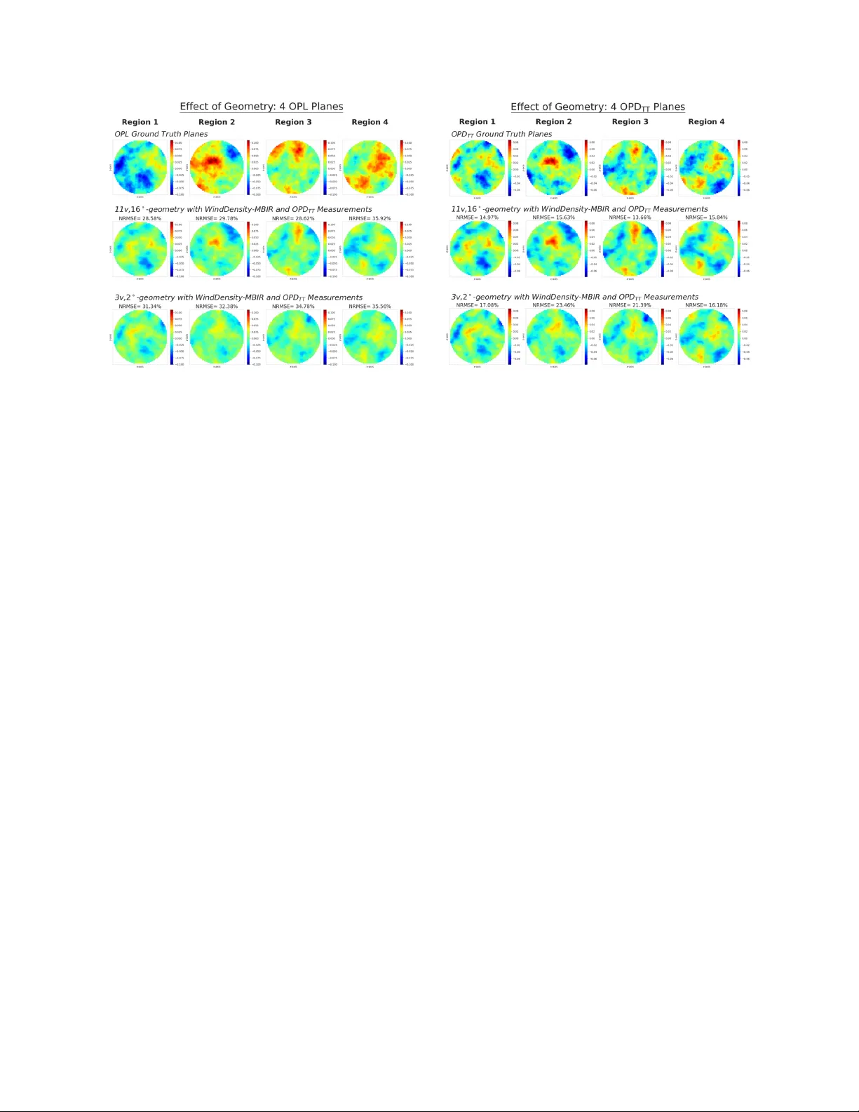
W indDensity-MBIR: Model-Based Iterativ e Reconstruction f or W ind T unnel 3D Density Estimation Karl J. W eisenbur ger a,* , Gregery T . Buzzard a , Charles A. Bouman b , Matthew R. K emnetz c a Purdue Univ ersity , Department of Mathematics, W est Lafayette, Indiana 47907, USA b Purdue Univ ersity , Departments of Electrical and Computer Engineering and Biomedical Engineering, W est Lafayette, Indiana 47907, USA c Air Force Institute of T echnology , Department of Engineering Physics, Wright-P atterson AFB, OH 45433, USA Abstract. Experimentalists often use wind tunnels to study aerodynamic turbulence, but most wind tunnel imag- ing techniques are limited in their ability to take non-in v asi ve 3D density measurements of turbulence. W avefront tomography is a technique that uses multiple wav efront measurements from various viewing angles to non-in v asiv ely measure the 3D density field of a turb ulent medium. Existing methods make strong assumptions, such as a spline basis representation, to address the ill-conditioned nature of this problem. W e formulate this problem as a Bayesian, sparse-view tomographic reconstruction problem and de velop a model-based iterativ e reconstruction algorithm for measuring the v olumetric 3D density field inside a wind tunnel. W e call this method W indDensity-MBIR and apply it using simulated data to difficult reconstruction scenarios with sparse data, small projection field of vie w , and limited angular extent. W indDensity-MBIR can recover high-order features in these scenarios within 10% to 25% error even when the tip, tilt, and piston are remov ed from the wa vefront measurements. Keyw ords: Non-in v asi v e W ind Tunnel Density Field Measurements, W avefront T omography , Coherent Imaging, Computed T omography , W ind T unnel Imaging, W avefront Sensing. * Karl J. W eisenburger , kweisen@purdue.edu 1 Introduction W av efront sensing is a class of imaging techniques that can be used to detect v ariations in a 3D density field due to high-speed airflo w. 1 When a coherent light source illuminates a turbulent airflo w , changes in refracti ve index due to v ariations in density can af fect the optical path length (OPL) of the light. W av efront sensing techniques such as digital holography or Shack-Hartmann wa v efront sensors can precisely measure the optical path dif ference (OPD) o ver a coherent beam’ s aperture, allowing researchers to non-in v asi v ely detect density variations for a turbulent airflo w . Ho we ver , OPD is a path-inte grated measurement along a line of sight and so does not yield point estimates of the underlying 3D density . Alternati vely , wind tunnel flow seeding can provide 3D point information, b ut it is in vasi v e and dif ficult to perform. 2 Computational fluid dynamics (CFD) Approv ed for public release; distrib ution is unlimited. Public Af fairs release appro v al # 2025-5579. 1 is non-in v asi ve and can model the 3D flo w dynamics, but CFD simulations often fail to match experimental tests. 3 , 4 W av efront tomography is an alternativ e non-in v asi v e method to estimate the 3D density field of a turbulent v olume. 5 While similar to parallel-beam x-ray tomography , wa vefront tomography for volumetric wind tunnel reconstruction is challenging is due to sparse views, limited field of vie w , limitations in angular extent, and incomplete projection information. T o capture the dynamic flo w field of wind tunnel turbulence, all wav efront measurements must be acquired at the same time. The physical constraints of imaging inside a wind tunnel limit the number and angular extent of wa v efront measurements that can be obtained simultaneously , turning this into a limited- angle, sparse view tomography problem. Furthermore, 2D OPD measurements are not complete projections of the turbulence refracti ve index because they lack the low order tip, tilt, and piston (TTP) information. By definition, OPD is blind to the mean OPL over the aperture (i.e., piston), and mechanical disturbances often contribute an unkno wn tip-tilt to the wa vefront, which effecti v ely obscures the tip-tilt contribution from the turbulence. In some cases, it is possible to recov er the complete projection information if the projection field of vie w (FO V) is wider than the medium of turbulence. 6 Ho we ver , for realistic wind tunnel experiments this is not possible because the FO V is limited by the beam diameter . Lastly , most wind tunnels hav e physical vie wing constraints that also restrict the angular extent of the projections, making it especially difficult to resolve features along one axis of the reconstruction. W av efront tomography has been e xplored extensi v ely in the field of microscopy for the goal of reconstructing the 3D sample refractiv e inde x. 7 While man y of the methods used in this field are designed for limited angle or sparse viewing scenarios, they do not consider scenarios where the object of reconstruction is significantly wider than the projection FO V . Furthermore, since the FO V Approv ed for public release; distrib ution is unlimited. Public Af fairs release appro v al # 2025-5579. 2 is wider than the sample, the additional projection information outside the sample (i.e., through the background reference medium) enables the recov ery of the complete projection information (i.e., TTP included) for the sample. Se veral wa vefront tomography methods have been dev eloped for wind-tunnel turbulence re- construction, but none of them use a Bayesian model-based reconstruction framework, which is well established in the field of x-ray tomography for regularization and artifact remo v al. 8 Some re- construction methods implicitly perform regularization by parameterizing the reconstruction with a lo w dimensional smooth orthogonal basis, 6 , 9 but these techniques do not use an e xplicit Bayesian prior model. Some sophisticated approaches hav e been de veloped to account for missing projec- tion information, which either incorporate additional reference information 6 , 9 or an iterativ e update loop, 10 , 11 but in all cases they do not use an explicit Bayesian prior model to smooth out the artifacts resulting from the unkno wn or incorrect projection information. Furthermore, most of the methods designed for turb ulence reconstruction are not designed for dif ficult imaging scenarios where the issues of sparse vie w , limited angle, small FO V , and unknown projection TTP are all present. For instance, some methods assume that the turbulent medium is radially symmetric, 9 , 10 which means that a single measurement can rev eal all 180 degrees of projection information. Alternati v ely , other methods assume that the turbulence stream induces a steady flow field, 12 which means that many measurements can be taken over the course of an extended time interv al. While some in v estigations into wind tunnel wa vefront tomography did assume scenarios with a se verely limited number of measurements, none of them considered cases where the angular extent was also sev erely limited (i.e., less than 90 de grees). 6 , 9 – 14 Furthermore, most experiments and simulations of wa vefront tomography assume that each projection FO V is significantly wider than the medium of turbulence. 9 – 14 Y . Zhang and G. A. Ruff specifically Approv ed for public release; distrib ution is unlimited. Public Af fairs release appro v al # 2025-5579. 3 in v estigated the issue of small FO V relati ve to the turb ulent medium and de veloped a method for estimating the unknown TTP. 6 Ho we ver , their technique assumes additional reference information, such as temperature probe measurements throughout the turb ulent medium, which is in v asi ve and dif ficult to obtain in practice. Some wav efront tomography techniques ov ercome the issues of sparse measurement data, small FO V , and limited angular e xtent by either using layered models of turbulence 15 – 18 or lower - dimensional basis representations 6 , 9 , 18 to reduce the complexity of the reconstruction problem. T omographic algorithms used in multi-conjugate adapti ve optics systems model atmospheric tur - bulence as se veral layered planes distributed at various elev ations. 15 – 17 Similarly , Klee et al. 18 demonstrated the experimental feasibility of tomographic wa vefront sensing for reconstructing two phase screens aligned along an optical bench. Their reconstruction algorithm also assumed a spline basis representation for each phase screen and solved for the basis coefficients. While layered models of turbulence are appropriate for many applications the y are not designed for vol- umetric reconstruction or capturing the spatially correlated features of wind tunnel turbulence. Furthermore, methods that use lower -dimensional basis representations are better posed, b ut their resolving capacity is limited to the features in the basis span. In this paper , we introduce W indDensity-MBIR, 19 a model-based iterativ e reconstruction (MBIR) method for non-inv asive estimation of the v olumetric density field inside a wind tunnel. W e formu- late the volumetric wa vefront tomography problem as parallel beam tomography and use e xisting parallel beam MBIR tomography algorithms and software 20 to estimate the unknown densities. W e sho w that W indDensity-MBIR can recov er high order features within 10% to 25% error ev en when there are fe w measurements, the angular extent is se v erely limited, and the measurements hav e TTP remov ed. W e compare W indDensity-MBIR to scale-corrected filtered back projection (FBP) and Approv ed for public release; distrib ution is unlimited. Public Af fairs release appro v al # 2025-5579. 4 find that MBIR significantly outperforms FBP . W e also inv estigate the effect of optical configura- tion on reconstruction quality and determine that reconstruction accurac y impro ves only when the maximum angular e xtent and the number of vie ws increase simultaneously . Lastly , we explore the deleterious effects of using non-ideal tip-tilt remov ed OPD measurements by performing recon- structions with ideal OPL measurements and comparing the two cases. In our simulations, roughly 95% of the additional error due to the unkno wn TTP is contained in lo wer order Zernike modes (of radial de gree 2 or less), which implies that W indDensity-MBIR applied for w av efront tomography is able to recov er high order modes e v en using TTP-remov ed OPD measurements. 2 Methodologies 2.1 Physical Model The physical quantity of interest is the 3D density field ρ inside the wind tunnel. Ho we ver , w a ve- front measurements are projections of the refractiv e inde x field n , which is related to the density field ρ via the Gladstone-Dale equation: 21 , 22 ρ (  r ) = n (  r ) − 1 K GD , (1) where K GD is the Gladestone-Dale constant and  r denotes a point in the volume. Thus, because wa v efront measurements are projections of refracti v e index, which is directly related to density via Eq. ( 1 ), for the rest of this paper we will focus on reconstructing the refracti ve inde x field n . A basic wav efront tomography measurement system would entail sev eral individually colli- mated coherent beam sources along with se v eral wa v efront detection systems. A wa vefront detec- tion system would include either a set of Shack–Hartmann wa vefront sensors or perhaps sev eral Approv ed for public release; distrib ution is unlimited. Public Af fairs release appro v al # 2025-5579. 5 Fig 1 Notional depiction of a wind tunnel wavefront tomograph y set up. digital holography set-ups each with their own reference beam. Figure 1 provides a notional rep- resentation of a possible wa v efront tomography set-up. W e denote a single projected ray through the v olume as γ j , where j indexes a particular pixel in a particular vie w . Then we model the OPL for a single ray as equal to the inte gral of the refracti v e index n along the path γ j gi ven by O P L j = Z γ j n (  r ) d  r , (2) where n (  r ) denotes the index of refraction at location  r . T o discretize Eq. ( 2 ), we replace the continuous refracti ve index v olume n with a discrete vectorized volume of N pixels x ∈ R N . W e replace the continuous integral along the path γ j with a linear forw ard projection giv en by the inner product with the column vector A j ∈ R N . Thus the discrete O P L is gi ven by A t j x ≈ Z γ j n (  r ) · d  r = O P L j . (3) Approv ed for public release; distrib ution is unlimited. Public Af fairs release appro v al # 2025-5579. 6 If the projected beams are collimated, the turbulence is weak, and the overall projection dis- tance is short, then we can approximate the beha vior of each projected beam as a b undle of parallel light rays that each follow a straight line path through the volume of turbulence. Under this ap- proximation, the linear operator A t j is the parallel beam forward projection for a single measured pixel in a single vie w . Thus, the complete forw ard model for the entire system of views is gi ven by y = Ax + W (4) where y is the set of all OPL measurements, A = [ A 0 , ..., A M − 1 ] t ∈ R M × N is the forward projec- tion operator for all vie ws, and W ∼ N (0 , σ y I ) is additi v e white Gaussian noise. Here M is the total number of pixels across all beam apertures. Also, note that y contains all the measurements for all projection vie ws and all angles. 2.2 Reconstruction Algorithm For a typical model-based approach, the final reconstruction ˆ x is the maximum a posteriori (MAP) estimate of the ground truth x . The MAP estimate is the reconstruction that jointly minimizes the forward model and prior model: ˆ x = arg min x {− log p ( y | x ) − log p ( x ) } = arg min x { f ( x ; y ) + h ( x ) } , (5) where f ( x ; y ) promotes the fit of Ax to the measured sinogram y , and h ( x ) represents the prior information on x . Using the parallel-beam frame work established in Sec. 2.1 , which assumes Gaussian measure- ment noise, we can write the forward model f ( x ; y ) for reconstructing the index of refraction x Approv ed for public release; distrib ution is unlimited. Public Af fairs release appro v al # 2025-5579. 7 as f ( x ; y ) = − log p ( y | x ) = 1 2 σ 2 y || y − Ax || 2 Λ + C, (6) where C is a constant independent of x , σ y is the assumed standard deviation of the measurement noise W , and Λ ∈ R M × M is a diagonal weight matrix (dependent on the optical configuration and y ) that defines the uncertainty for each OPL projection y j . For our prior model h ( x ) we chose the generalized Gaussian Marko v random field (GGMRF). 23 T echnically , to achiev e the true MAP estimate, the prior model must equal (up to a constant) the negati ve log prior distrib ution for the v olume being reconstructed h ( x ) = − log p ( x ) + C ′ . How- e ver , it is often suf ficient if h ( x ) simply captures some reasonable statistical assumptions about the volume being reconstructed. In our case, we assume that the volume x is smooth, having minimal v ariation between most adjacent vox els. The GGMRF model can implement these assumptions while also providing flexibility to tune the amount regularization. W e use the existing MBIR- J AX package 20 to solve Eq. ( 5 ) since it has implementations of the parallel beam forward model in Eq. ( 6 ) and the GGMRF prior model. The MBIRJ AX package solves Eq. ( 5 ) with vectorized coordinate descent. 24 2.3 Using Non-Ideal T ip-tilt Removed Optical P ath Differ ence While the reconstruction problem giv en by Eq. ( 5 ) assumes that the measurement for each beam is OPL, this is not experimentally feasible. Standard wa v efront detection techniques, such as digital holograph y or Shack–Hartmann w a vefront sensors, measure only the w a vefront OPD, i.e., the mean-remov ed OPL. Furthermore, for measurements through wind tunnel turbulence, most OPD sensing techniques cannot reco v er the tip-tilt (i.e., the linear trend across the aperture) from the turbulence because this is obscured by the tip-tilt contributions from mechanical disturbances. Approv ed for public release; distrib ution is unlimited. Public Af fairs release appro v al # 2025-5579. 8 This means that for e xperimental measurements of turbulence in wind tunnels, the tip-tilt is usually remov ed from the OPD. The tip-tilt remo ved OPD measurement, OPD TT , can be expressed as O P D T T ( u, v ) = O P L ( u, v ) − ( au + bv + c ) (7) where ( a, b, c ) = arg min a,b,c ∥ O P L ( u, v ) − ( au + bv + c ) ∥ 2 . (8) Thus, for the primary analysis of our algorithm, we used simulated OPD TT measurements as the input for our algorithm instead of OPL. Because the forward model gi ven by Eq. ( 6 ) assumes that the measurements y are OPL, using OPD TT instead of OPL introduces model mismatch and degrades reconstruction quality . T o determine the effects of model mismatch due to using OPD TT instead of OPL measurements, we also performed a secondary analysis in Sec. 3.3 where we simulated reconstructions with OPL measurements. Comparing the error between reconstructing with OPD TT and reconstructing with OPL indicated that the additional error due model mismatch is mostly contained in lo wer order Zernike modes. 2.4 Simulation and V alidation Pr ocedur e 2.4.1 Atmospheric phase volume generation T o validate the effecti v eness of W indDensity-MBIR, we randomly generated 3D phase volumes based on the K olmogoro v phase power spectral density (PSD). W e chose to use Kolmogoro v at- mospheric turbulence for our simulations because it is well understood and straightforward to model. T o generate 3D phase volumes, we extend the commonly used Fourier transform method for Approv ed for public release; distrib ution is unlimited. Public Af fairs release appro v al # 2025-5579. 9 generating 2D atmospheric phase screens 25 to generate 3D v olumes. W e make use of the modified von K ´ arm ´ an phase PSD: Φ mv K ϕ ( κ ) = 0 . 49 r − 5 3 0 exp {− κ 2 /κ 2 m } ( κ 2 + κ 2 0 ) 11 6 (9) where r 0 is the Fried’ s coherence length in meters, κ m and κ 0 are the high and lo w frequency scale parameters, and κ is the angular wa v e number , all in m − 1 . T o generate a v olume with ph ysical dimensions ( L, W, H ) in meters on a finite grid with PSD gi ven by ( 9 ), we first consider the phase v olume x as a Fourier series: x (  r ) = X  n ∈ Z 3 c  n exp { j 2 π ⟨ F  n,  r ⟩} (10) where F = diag ([1 /L, 1 /W, 1 /H ]) is a diagonal matrix of the frequenc y spacings. From here we model the Fourier coef ficients as ha ving Gaussian real and imaginary parts, ℜ{ c  n } ∼ N (0 , σ 2  n ) and ℑ{ c  n } ∼ N (0 , σ 2  n ) , (11) each with v ariance σ 2  n specified by Φ mv K ϕ , σ 2  n = Φ mv K ϕ ( ∥ F  n ∥ 2 ) LW H . (12) Follo wing the approach used by Schmidt, 25 we implement Eqs. ( 10 ) - ( 12 ) in software with pseudo- random number generation and the fast F ourier transform. Importantly , we are not attempting to simulate statistically accurate ground truth refracti v e in- dex volumes. The K olmogoro v phase PSD models the 2D phase fluctuations for a coherent beam Approv ed for public release; distrib ution is unlimited. Public Af fairs release appro v al # 2025-5579. 10 passing through a medium of atmospheric turb ulence. It does not model a volume of atmospheric refracti ve index. For the purpose of performing a basic test of W indDensity-MBIR, which was ultimately designed for aero-optical turb ulence in a wind tunnel, our goal was simply to generate statistically independent v olumes containing random isotropic turb ulent structures that are reason- ably sized. The modified v on K ´ arm ´ an PSD for phase screens is appropriate for this goal because the inner and outer scale parameters ( L 0 = 2 π /κ 0 and l 0 = 2 π /κ m ) allow us to easily control the size range of the turbulent structures. For all tests done in this paper , we used r 0 = 0 . 5 cm, L 0 = 2 cm, and l 0 = 0 . 2.4.2 Simulating OPL and tip-tilt r emo ved OPD measurements For the results shown in this paper , we tested 40 different optical configurations, varying both the number of beams and the overall angular extent. For the total number of beams, we tested 3 , 5 , 7 , 9 , and 11 beams. For the total angular extent of we tested 2 ◦ , 4 ◦ , 6 ◦ , 8 ◦ , 10 ◦ , 12 ◦ , 14 ◦ , and 16 ◦ . In every case, the optical ax es of the beams lie on a single plane perpendicular to the axis of rotation. Furthermore, for ev ery configuration, the beam angles are uniformly distributed across the total angular extent, which means the angular separation between adjacent beams is always angular extent / ( number of views − 1) . Figure 2 shows the beam paths for one geometry with the narro west angular extent and fewest views and another geometry with the widest angular extent and most vie ws. For a gi v en simulated volume of refracti v e index x and an optical configuration, computing the OPL and the tip-tilt remov ed OPD is relativ ely straightforward. Following Eq. ( 3 ), we compute the OPL forw ard projection for each beam as the integral of x along all rays parallel to the beam’ s optical axis. W e use the MBIRJ AX forward projection operator 20 to perform this computation. Approv ed for public release; distrib ution is unlimited. Public Af fairs release appro v al # 2025-5579. 11 (a) (b) Fig 2 Overhead view of (a) the geometry with the fewest vie ws and narro west angular extent and (b) the geometry with the most views and widest angular e xtent. Then we set all values outside the beam’ s predefined FO V to zero. For all results shown in this paper , we set the beam FO V to be a 2 cm disk. Finally , we compute the OPD TT (tip-tilt remov ed OPD) by fitting a plane to the OPL and then subtracting it from the OPL (see Eq. ( 8 ) and ( 7 )). 2.4.3 Resolution r eduction and con ventions for err or analysis Throughout this paper we use the term “depth axis” to refer to the line that bisects the largest angular range from which we take our measurements. This axis is the same for all our tests and is perpendicular to both windo ws on either side of the wind tunnel test region (see Fig. 3 ). For this paper , we restrict our region of interest (R OI) to the region of turb ulence that the central beam passes through. F or our set up, this region is a cylinder extending along the depth axis, perpendicular to both windows (see Fig. 4 ). All error computations and visualizations in this paper will be restricted to this region. For visualization purposes (and to test the limits of depth axis resolution using WindDens ity- MBIR) we often reduce the resolution along the depth axis by computing the OPL for a few regions along this axis. T o do this we simply divide each full resolution volume (reconstruction and ground Approv ed for public release; distrib ution is unlimited. Public Af fairs release appro v al # 2025-5579. 12 Fig 3 Schematic sho wing the depth axis relati ve to the location of the windo ws. The red shaded region designates range of possible view angles. Fig 4 Example depiction of the integration process for reducing the resolution along the depth axis to 3 OPL planes. The windows in Fig. 3 correspond to the left and right ends of this v olume. The red cylinder represents our chosen reconstruction R OI, i.e., the path of the central beam. truth) into a specified number of equally sized re gions along the depth axis and then integrate each of them along the depth axis. Figure 4 shows a visualization of this process for the case of reducing the resolution to 3 OPL planes along the depth axis. Note that in some cases we will also consider the tip-tilt remov ed OPD contrib utions from each region, which we will refer to as OPD TT planes. T o ev aluate the reconstruction accuracy relati ve to the simulated ground truth, we use stable range normalization for our normalized root mean squared error (NRMSE) computations. This Approv ed for public release; distrib ution is unlimited. Public Af fairs release appro v al # 2025-5579. 13 Fig 5 The first 45 Zernike modes ordered by radial degree. means that we normalize the root mean squared error by di viding by the inner 90th interpercentile range of the ground truth volume. 2.4.4 Zernike expansion Figure 5 displays the first 45 Zernike modes, organized into 9 radial degrees, from the Zernike basis, which is an orthogonal basis using the L 2 inner product o v er the unit disk. W e use this basis in Sec. 3.2.2 and 3.3.1 to analyze the lo w degree energy distribution of W indDensity-MBIR’ s reconstruction error . T o do this in the case of kno wn ground truth x and reconstruction ˆ x , we apply depth axis resolution reduction to x and ˆ x − x as in the previous section. W e then project each resulting 2D region onto the span of one radial de gree to obtain an error image, ˆ x err d,j for degree d and region j . W e then report P j ∥ ˆ x err d,j ∥ 2 / P j ∥ x j ∥ 2 as the normalized mean-squared error for that degree. 3 Results In this section we in vestigate the performance of W indDensity-MBIR using a v ariety of e valuation methods. For all of the simulations except the in vestigation of geometry configurations, we use the 7-vie w geometry with 8 degrees of angular e xtent. This geometry is not numerically optimal, b ut Approv ed for public release; distrib ution is unlimited. Public Af fairs release appro v al # 2025-5579. 14 we chose it as an approximate limit of physical feasibility . For con venience, we will refer to the geometry with N views and θ angular e xtent as the “ N v , θ ◦ -geometry”. 3.1 Comparison to Scale-Corr ected FBP Scale-corrected FBP is a version of standard FBP that is scaled to better match the measured sinogram. The scale-corrected FBP is given by ˆ x F B P cor rected = α · ˆ x F B P . (13) where ˆ x F B P is the standard FBP reconstruction and the scaling coef ficient α is giv en by α = ⟨ y , A ˆ x F B P ⟩ ∥ A ˆ x F B P ∥ 2 2 . (14) Thus, computing the scale-corrected FBP reconstruction requires an additional forward projection of the standard FBP reconstruction (i.e., A ˆ x F B P ) but in return gi ves the scaling that minimizes the mean-squared error between the sinogram and the projected reconstruction. Figure 6 shows example reconstructions comparing scale-corrected FBP to W indDensity-MBIR using the 7v ,8 ◦ -geometry . Even with scale correction, FBP produces poor results in comparison to MBIR because it is ill-suited for sparse reconstruction. T able 1 sho ws the a verage NRMSE of 3 methods for reconstructing 4 OPD TT planes, using 3 representati ve geometries. The av erage NRMSE was computed for 100 different reconstructions. Here we see that scale-corrected FBP has lo wer NRMSE than standard FBP , by a factor of about 10, but is still inferior to MBIR. Approv ed for public release; distrib ution is unlimited. Public Af fairs release appro v al # 2025-5579. 15 Fig 6 Effect of reconstruction method on reconstruction quality . Example reconstructions of 4 OPD TT planes along the depth axis using the 7v ,8 ◦ -geometry . The top row shows ground truth, the middle ro w shows WindDensity-MBIR, and the bottom ro w shows scale-corrected FBP . The limited measurements lead to high-frequency artifacts in the scale- corrected FBP reconstruction. T able 1 NRMSE of FBP and MBIR for Reconstructing 4 OPD TT planes, av eraged ov er 100 samples Method Geometry 3v ,2 ◦ 7v ,8 ◦ 11v ,16 ◦ FBP 5.689 2.191 1.734 Scale-Corrected FBP 0.266 0.227 0.219 W indDensity-MBIR (ours) 0.215 0.179 0.168 3.2 Reconstruction Err or Analysis 3.2.1 Err or as a function of viewing geometry Figure 7 shows the NRMSE of W indDensity-MBIR for each of the 40 vie wing configurations, av eraged o ver reconstructions of 100 simulated volumes of turb ulence. Plot (a) shows the NRMSE for a full resolution reconstruction (v oxel depth equal to vox el width) and thus re veals the essential relationship between the viewing configuration and reconstruction accuracy . Plot (b) shows the NRMSE for a resolution of 4 OPL planes, which is a more feasible resolution for achieving high accuracy . While the y -axis scaling is different between the (a) and (b) plots, the overall trend Approv ed for public release; distrib ution is unlimited. Public Af fairs release appro v al # 2025-5579. 16 (a) (b) Fig 7 Plots of av erage NRMSE relative to the total angular extent for the vie wing configuration: (a) reconstructing full resolution and (b) reconstructing 4 OPL planes. The red circles designate geometries with 2 degrees of angular separation between adjacent vie ws and highlight the decrease in error as angular e xtent increases simultaneously with number of views. is the same. Both plots highlight the importance of balancing angular extent with view overlap. Particularly in (b), the reconstruction quality consistently improv es only when we increase the number of vie ws and the total angular extent simultaneously . Figure 7 indicates that for 2 ◦ and 4 ◦ of ov erall angular extent, increasing the views can only marginally impro ve the accuracy . Furthermore, when the number of vie ws is limited to 3 or 5, in- creasing angular e xtent can actually de grade the reconstruction accuracy . This is because increas- ing the overall angular extent without increasing the number of views is equiv alent to increasing the total number of unkno wns without increasing the number of measurements. Figure 8 sho ws two edge case geometries (3v ,2 ◦ and 3v ,16 ◦ ) that illustrate the fundamental trade-of f between angular extent and vie w ov erlap. T o in vestigate this trade-of f, we reconstructed 3000 different v olumes of turbulence for each of these viewing configurations. W e then reduced the resolution to 5 OPL planes along the depth axis and computed the error individually for each plane. Approv ed for public release; distrib ution is unlimited. Public Af fairs release appro v al # 2025-5579. 17 (a) (b) Fig 8 Overhead vie w of two edge case geometries: (a) the 3v ,2 ◦ -geometry and (b) the 3v ,16 ◦ -geometry (right). Note, the R OI in green is broken into the 5 re gions that are reduced to 5 OPL planes for the experiment. Figure 9 plots the NRMSE for these two geometries as a function of depth of the region of the reconstructed OPL plane, a v eraged ov er the 3000 reconstructions. The narro w 3v ,2 ◦ -geometry reconstructs the OPL contributions from the outermost regions significantly better than the wide 3v ,16 ◦ -geometry . This indicates that the views for the wider geometry do not ov erlap enough o v er the outermost regions. Con versely , the narro w geometry has greater error for the central OPL plane, which indicates that the 3 beams for the narro w geometry ov erlap too much ov er this central region. Thus, each beam contributes v ery little unique information for reconstructing this re gion. 3.2.2 Zernike expansion err or analysis Figure 10 shows the normalized mean squared error (MSE) for OPL reconstruction using OPD TT measurements, as a function of Zernike radial degree, for the best (11v ,16 ◦ ) and worst (3v ,2 ◦ ) geometries of those we in vestigated (see Fig. 2 ). The normalized MSE is P j ∥ ˆ x err d,j ∥ 2 / P j ∥ x j ∥ 2 as described in Sec. 2.4.4 , and we a v erage o ver 1000 samples. Note that since lo w order de grees tend to contain more ener gy in general, we expect to see some ener gy decay from lo w to high order degrees. Approv ed for public release; distrib ution is unlimited. Public Af fairs release appro v al # 2025-5579. 18 Fig 9 NRMSE as a function of re gion along the depth axis, averaged over 3000 reconstructions. Error bars designate 2 standard deviations for the mean estimate. The blue plot has the highest NRMSE for the central region because there is too much ov erlap over this region. The orange plot has the highest error for the outermost regions because there is not enough ov erlap ov er these regions. Fig 10 Normalized MSE as a function of Zernik e radial de gree for reconstructing 4 OPL planes with OPD TT mea- surements, av eraged ov er 1000 samples. The data-rich 11v ,16 ◦ -geometry (bro wn) sho ws significantly lower error at high degrees than the data-poor 3v ,2 ◦ -geometry . Both geometries have large errors in degrees 0 and 1, which are not measured in OPD TT . Figure 10 indicates that lowest order Zernike modes (particularly TTP) contain the largest percentage of the error energy . The TTP modes account for approximately 60% of the overall MSE for the 11v ,16 ◦ -geometry (bro wn) and 51% for the 3v ,2 ◦ -geometry (blue). The lar ge errors in TTP modes are expected, giv en that the OPD TT measurements do not detect TTP . This conclusion is further validated by the fact that the better geometry only marginally outperforms the worse Approv ed for public release; distrib ution is unlimited. Public Af fairs release appro v al # 2025-5579. 19 (a) (b) Fig 11 Effect of geometric configuration on reconstruction quality . Example reconstructions of 4 planes: (a) recon- structions of 4 OPL planes and (b) reconstructions of 4 OPD TT planes, all using W indDensity-MBIR. The top row shows ground truth, the middle ro w uses the 11v ,16 ◦ -geometry , and bottom row uses the 3v ,2 ◦ -geometry . geometry for the TTP modes. Figure 11 compares reconstructed planes to ground truth planes. Display (a) shows the OPL contributions from each region, while display (b) shows the OPD TT contributions from each region. For both (a) and (b) the top ro w is the ground truth, the middle row is the reconstruction using the best geometry , and the bottom row is the reconstruction using the worst geometry . W e see that the visual match and NRMSE are much better when we reconstruct the OPD TT rather than OPL, which contains unmeasured TTP information. 3.2.3 Depth r esolution err or analysis Figure 12 plots the a verage reconstruction NRMSE relati v e to the number of OPL or OPD TT planes along the depth axis. The plots are the result of performing 100 dif ferent reconstructions with the 7v ,8 ◦ -geometry and then computing the NRMSE for v arious resolutions along the depth axis. W e can see that the reconstruction quality de grades quickly as we increase the resolution from 2 to 5 planes. Approv ed for public release; distrib ution is unlimited. Public Af fairs release appro v al # 2025-5579. 20 Fig 12 NRMSE (averaged over 100 samples) as a function of number of reconstruction planes using the 7v ,8 ◦ - geometry and OPD TT measurements. The blue curve shows OPL reconstruction, while the orange shows OPD TT reconstruction. Due to the missing TTP information, the OPL reconstruction shows consistently higher error , and both curves sho w a significant increase in error from 2 to 5 planes. Figure 12 indicates that, to achie ve less than 20% error , we can expect to accurately reconstruct at most 4 OPD TT planes. Based on qualitativ e experience, we have found that when the error exceeds 20%, the o v erall visual match starts to degrade significantly . 3.3 Model Mismatch Effects fr om Using T ip-tilt Removed Measur ements For our secondary analysis, we attempt to quantify the error due to model mismatch from us- ing OPD TT measurements instead of OPL. T o do this, we perform additional reconstructions with simulated ideal OPL measurements and compare to our earlier reconstructions with OPD TT mea- surements. The main conclusion from our in v estigation is that the vast majority of the additional error due to model mismatch from using non-ideal OPD TT measurements is contained in the low order TTP modes (radial degrees 0 and 1) of the reconstruction, with some small additional error contained in radial degree 2. In particular , for solely recov ering OPD TT planes along the depth axis, reconstructing with OPD TT measurements is only mar ginally worse than reconstructing with Approv ed for public release; distrib ution is unlimited. Public Af fairs release appro v al # 2025-5579. 21 Fig 13 Results analogous to Fig. 10 for reconstructing 4 OPL planes, but comparing the effect of OPL measurements versus OPD TT measurements. The primary difference in error is in the low order degrees 0 and 1, which are not measured in OPD TT . Roughly 95% of the additional error from removing TTP (model-mismatch) is concentrated in degrees 0, 1, 2. OPL. 3.3.1 Zernike analysis Figure 13 shows the Zernike modal energy distribution of the normalized mean squared recon- struction error for both reconstructing with OPL measurements and reconstructing with OPD TT measurements. For this result, we used the 7v ,8 ◦ -geometry . W e can see that Zernike modes of radial degree 0 and 1 (i.e., TTP) contain most of the additional error , which we should expect since the OPD TT measurements do not included TTP . T o be precise, on av erage 80% of the additional mean squared error due to using OPD TT measurements instead of OPL is contained in Zernike modes of radial degree 0 and 1. Furthermore, the majority of the higher order ef fects due to model mismatch are accounted for by radial de gree 2, which on av erage contained 15% of the dif ference in MSE between OPL tomography and OPD TT tomography . Figure 14 compares (a) OPL and (b) OPD TT reconstructions using OPL measurements and OPD TT measurements. W e see that the OPL reconstructions using OPD TT measurements failed to capture certain features that were captured in OPL reconstructions using OPL measurements. Approv ed for public release; distrib ution is unlimited. Public Af fairs release appro v al # 2025-5579. 22 (a) (b) Fig 14 Effect of OPL versus OPD TT measurements. Example reconstructions of 4 planes along the depth axis using the 7v , 8 ◦ geometry: (a) reconstruction of 4 OPL planes and (b) reconstruction of 4 OPD TT planes. The top ro w sho ws ground truth, the middle row uses OPL measurements, and the bottom ro w uses OPD TT measurements. Note the TTP information in OPL measurements significantly improves the OPL reconstructions but only marginally improves the OPD TT reconstructions. Ho we ver , the OPD TT reconstructions using either OPL or OPD TT look nearly identical and hav e comparable NRMSE. 3.3.2 Resolution analysis Figure 15 plots the NRMSE as a function of depth axis resolution for the case of using OPL mea- surements (blue) and the case of using OPD TT measurements (orange). Plot (a) sho ws the NRMSE for reconstructing OPL, while plot (b) shows the NRMSE for reconstructing OPD TT planes, all using the 7v ,8 ◦ -geometry . The dif ference between plots (a) and (b) of Fig. 15 confirms that, re- gardless of resolution, if we reconstruct OPD TT planes, then using OPL measurements is only marginally w orse than using OPD TT measurements. Approv ed for public release; distrib ution is unlimited. Public Af fairs release appro v al # 2025-5579. 23 (a) (b) Fig 15 NRMSE as a function of depth axis resolution: (a) NRMSE for reconstructing OPL planes and (b) NRMSE for reconstructing OPD TT planes. For reconstructing OPD TT planes, re gardless of resolution, using OPD TT measurements is only marginally w orse than using OPL measurements. 4 Conclusion W ind tunnels offer a controlled setting for studying aerodynamic turbulence, but obtaining non- in v asi v e 3D density measurements remains challenging. Most basic techniques, such as optical path difference imaging, provide only 2D data and miss the 3D turb ulence structure. In vasi v e methods like flo w seeding are difficult to perform, while CFD models often div erge from experi- ments. This highlights the need for tomographic approaches that non-in v asi v ely measure the 3D density field. In this paper , we introduced WindDensity-MBIR, an MBIR tomography method for recon- structing the 3D refracti ve index inside a wind tunnel. Our simulations show that W indDensity- MBIR can reconstruct the non-TTP (higher order) features of 2 to 6 regions along the depth axis with error between 10% to 25%, on av erage, assuming sufficient vie ws and angular e xtent. Increas- ing both the number of views and angular extent simultaneously impro v es results, but increasing angular extent without increasing the number of vie ws can make the reconstruction quality worse. For our secondary analysis we compared reconstructing with OPL vie ws to tip-tilt remo ved OPD vie ws, and this indicated that the additional error due to model mismatch (from using non-ideal Approv ed for public release; distrib ution is unlimited. Public Af fairs release appro v al # 2025-5579. 24 tip-tilt removed OPD) is contained primarily in lo wer order Zernike modes, while higher-order features remain recov erable. These findings highlight the potential for model-based methods to perform non-in v asi v e density measurements. 5 Disclosures The authors declare that there are no financial interests, commercial af filiations, or other potential conflicts of interest that could hav e influenced the objecti vity of this research or the writing of this paper . The vie ws e xpressed are those of the author and do not necessarily reflect the official polic y or position of the Department of the Air F orce, the Department of Defense, or the U.S. Go vernment. Approv ed for public release; distrib ution is unlimited. Public Af f airs release appro v al # 2025-5579. Code, Data, and Materials A v ailability The code used to generate the figures and results is av ailable in a Github repository linked in Ref. 19 . The simulated data used to validate our method is not av ailable due to memory storage constraints. Acknowledgments C.A.B. was partially supported by the Sho walter T rust. K.J.W ., G.T .B., and C.A.B. were partially supported by AFRL/RDKL F A9451-20-2-0008. The authors would like to thank the Show alter family and the United States Air F orce for supporting this research. Approv ed for public release; distrib ution is unlimited. Public Af fairs release appro v al # 2025-5579. 25 Refer ences 1 E. J. Jumper and S. Gordeye v , “Physics and measurement of aero-optical ef fects: Past and present, ” Annual Review of Fluid Mechanics 49 (V olume 49, 2017), 419–441 (2017). 2 P . Danehy , J. W eisberger , C. Johansen, et al. , “Non-intrusiv e measurement techniques for flo w characterization of hypersonic wind tunnels, ” in Thermal and Fluids Analysis W orkshop (TF A WS 2019) , N ASA, (Ne wport Ne ws, V irginia, USA) (2019). 3 J. W ells, M. Kalensky , R. M. Rennie, et al. , “Experimental and computational in vestig ation of Shack–Hartmann w a vefront sensor measurements through a free shear layer, ” Optical En- gineering 63 (1), 014108 (2024). 4 A. A. Oliv a, T . E. DeFoor , and R. M. Rennie, “Computational in v estigation of aero-optical discrepancies in a free shear layer, ” in Uncon ventional Imaging, Sensing, and Adaptive Optics 2025 , J. J. Dolne, S. R. Bose-Pillai, and M. Kalensky , Eds., 13619 , 136190N, International Society for Optics and Photonics, SPIE (2025). 5 L. Hesselink, “Optical tomography , ” in Handbook of Flow V isualization , W .-J. Y ang, Ed., 307–328, Routledge, 2 ed. (2001). 6 Y . Zhang and G. A. Ruff, “Reconstruction of refractiv e index fields by using relati ve fringe data, ” Appl. Opt. 32 , 2921–2926 (1993). 7 V . Balasubramani, A. Ku ´ s, H.-Y . T u, et al. , “Holographic tomography: techniques and biomedical applications [in vited], ” Appl. Opt. 60 , B65–B80 (2021). 8 L. Liu, “Model-based iterati ve reconstruction: A promising algorithm for today’ s computed tomography imaging, ” Journal of Medical Imaging and Radiation Sciences 45 (2), 131–136 (2014). Approv ed for public release; distrib ution is unlimited. Public Af fairs release appro v al # 2025-5579. 26 9 C. T ian, Y . Y ang, Y . Zhuo, et al. , “T omographic reconstruction of three-dimensional refractiv e index fields by use of a regularized phase-tracking technique and a polynomial approximation method, ” Appl. Opt. 50 , 6495–6504 (2011). 10 C. M. V est and I. Prikryl, “T omography by iterativ e con volution: empirical study and appli- cation to interferometry , ” Appl. Opt. 23 , 2433–2440 (1984). 11 S. S. Cha and H. Sun, “T omography for reconstructing continuous fields from ill-posed mul- tidirectional interferometric data, ” Appl. Opt. 29 , 251–258 (1990). 12 C. S ¨ oller , R. W enskus, P . Middendorf, et al. , “Interferometric tomography for flo w visual- ization of density fields in supersonic jets and con v ecti v e flow , ” Appl. Opt. 33 , 2921–2932 (1994). 13 M. C. Roggemann, B. M. W elsh, P . J. Gardner , et al. , “Sensing three-dimensional index-of- refraction variations by means of optical wav efront sensor measurements and tomographic reconstruction, ” Optical Engineering 34 (5), 1374 – 1384 (1995). 14 L. McMackin, R. J. Hugo, R. E. Pierson, et al. , “High speed optical tomography system for imaging dynamic transparent media, ” Opt. Expr ess 1 , 302–311 (1997). 15 F . Rigaut and B. Neichel, “Multiconjugate adapti v e optics for astronomy , ” (2020). 16 Zhang, Lingxiao, Zhang, Lanqiang, Zhong, Libo, et al. , “Deep tomography for the three- dimensional atmospheric turbulence w a vefront aberration, ” A&A 687 , A182 (2024). 17 M. Hart, S. Jefferies, and D. Hope, “T omographic wa ve-front sensing with a single guide star, ” in Uncon ventional Imaging and W avefr ont Sensing XII , J. J. Dolne, T . J. Karr , and D. C. Dayton, Eds., 9982 , 998207, International Society for Optics and Photonics, SPIE (2016). Approv ed for public release; distrib ution is unlimited. Public Af fairs release appro v al # 2025-5579. 27 18 A. Klee, S. T . Thurman, and T . Alley , “Digital holographic tomography for path-resolved turbulence measurements, ” in Uncon ventional Imaging and Adaptive Optics 2021 , J. J. Dolne and M. F . Spencer , Eds., 11836 , 118360F , International Society for Optics and Photonics, SPIE (2021). 19 W . J. Karl, G. T . Buzzard, C. A. Bouman, et al. , “W indDensity-MBIR. ” Soft- ware library av ailable from https://github.com/Karl- Weisenburger/ WindDensity- MBIR (2025). 20 C. A. Bouman and G. T . Buzzard, “MBIRJ AX: High-performance tomographic reconstruc- tion. ” Software library av ailable from https://github.com/cabouman/mbirjax (2024). 21 J. H. Gladstone and T . P . Dale, “Researches on the refraction, dispersion, and sensiti veness of liquids, ” Philosophical T r ansactions of the Royal Society of London 153 , 317–343 (1863). 22 J. H. B. Anderson, “Experimental determination of the gladstone-dale constants for dissoci- ating oxygen, ” The Physics of Fluids 12 , I–57–I–60 (1969). 23 J.-B. Thibault, K. D. Sauer , C. A. Bouman, et al. , “ A three-dimensional statistical approach to improv ed image quality for multislice helical ct, ” Medical Physics 34 (11), 4526–4544 (2007). 24 C. A. Bouman and G. T . Buzzard, “V ectorized coordinate descent for fast ct reconstruction. ” Poster presented at 2024 CVPR W orkshop: Computer V ision for Science (2024). 25 J. D. Schmidt and S. of Photo-optical Instrumentation Engineers., Numerical simulation of optical wave pr opagation with examples in MATLAB , 149–184. Press monograph ; 199, SPIE, Bellingham, W ash (2010). Approv ed for public release; distrib ution is unlimited. Public Af fairs release appro v al # 2025-5579. 28 Karl J. W eisenburger is Mathematics PhD candidate at Purdue Uni versity . He receiv ed his BS in applied mathematics from Hillsdale College in 2022. His current research interests include computational imaging and aero-optics. List of Figures 1 Notional depiction of a wind tunnel wa v efront tomography set up. 2 Overhead view of (a) the geometry with the fewest vie ws and narro west angular extent and (b) the geometry with the most vie ws and widest angular e xtent. 3 Schematic showing the depth axis relati ve to the location of the windows. The red shaded region designates range of possible vie w angles. 4 Example depiction of the integration process for reducing the resolution along the depth axis to 3 OPL planes. The windows in Fig. 3 correspond to the left and right ends of this volume. The red cylinder represents our chosen reconstruction R OI, i.e., the path of the central beam. 5 The first 45 Zernike modes ordered by radial de gree. 6 Ef fect of reconstruction method on reconstruction quality . Example reconstruc- tions of 4 OPD TT planes along the depth axis using the 7v ,8 ◦ -geometry . The top ro w sho ws ground truth, the middle row shows W indDensity-MBIR, and the bottom ro w sho ws scale-corrected FBP . The limited measurements lead to high-frequency artifacts in the scale-corrected FBP reconstruction. 29 7 Plots of av erage NRMSE relativ e to the total angular extent for the viewing con- figuration: (a) reconstructing full resolution and (b) reconstructing 4 OPL planes. The red circles designate geometries with 2 de grees of angular separation between adjacent views and highlight the decrease in error as angular extent increases si- multaneously with number of vie ws. 8 Overhead view of two edge case geometries: (a) the 3v ,2 ◦ -geometry and (b) the 3v ,16 ◦ -geometry (right). Note, the R OI in green is broken into the 5 regions that are reduced to 5 OPL planes for the experiment. 9 NRMSE as a function of region along the depth axis, av eraged over 3000 recon- structions. Error bars designate 2 standard deviations for the mean estimate. The blue plot has the highest NRMSE for the central re gion because there is too much ov erlap over this region. The orange plot has the highest error for the outermost regions because there is not enough o v erlap ov er these regions. 10 Normalized MSE as a function of Zernike radial degree for reconstructing 4 OPL planes with OPD TT measurements, av eraged ov er 1000 samples. The data-rich 11v ,16 ◦ -geometry (bro wn) shows significantly lo wer error at high degrees than the data-poor 3v ,2 ◦ -geometry . Both geometries hav e large errors in degrees 0 and 1, which are not measured in OPD TT . 11 Ef fect of geometric configuration on reconstruction quality . Example reconstruc- tions of 4 planes: (a) reconstructions of 4 OPL planes and (b) reconstructions of 4 OPD TT planes, all using W indDensity-MBIR. The top ro w shows ground truth, the middle ro w uses the 11v ,16 ◦ -geometry , and bottom row uses the 3v ,2 ◦ -geometry . Approv ed for public release; distrib ution is unlimited. Public Af fairs release appro v al # 2025-5579. 30 12 NRMSE (av eraged over 100 samples) as a function of number of reconstruction planes using the 7v ,8 ◦ -geometry and OPD TT measurements. The blue curve sho ws OPL reconstruction, while the orange shows OPD TT reconstruction. Due to the missing TTP information, the OPL reconstruction sho ws consistently higher error , and both curves sho w a significant increase in error from 2 to 5 planes. 13 Results analogous to Fig. 10 for reconstructing 4 OPL planes, but comparing the ef fect of OPL measurements versus OPD TT measurements. The primary difference in error is in the low order degrees 0 and 1, which are not measured in OPD TT . Roughly 95% of the additional error from removing TTP (model-mismatch) is concentrated in degrees 0, 1, 2. 14 Ef fect of OPL v ersus OPD TT measurements. Example reconstructions of 4 planes along the depth axis using the 7v , 8 ◦ geometry: (a) reconstruction of 4 OPL planes and (b) reconstruction of 4 OPD TT planes. The top row sho ws ground truth, the middle ro w uses OPL measurements, and the bottom row uses OPD TT measure- ments. Note the TTP information in OPL m easurements significantly impro v es the OPL reconstructions but only mar ginally impro ves the OPD TT reconstructions. 15 NRMSE as a function of depth axis resolution: (a) NRMSE for reconstructing OPL planes and (b) NRMSE for reconstructing OPD TT planes. For reconstruct- ing OPD TT planes, regardless of resolution, using OPD TT measurements is only marginally w orse than using OPL measurements. 31 List of T ables 1 NRMSE of FBP and MBIR for Reconstructing 4 OPD TT planes, av eraged o ver 100 samples Approv ed for public release; distrib ution is unlimited. Public Af fairs release appro v al # 2025-5579. 32