Hybrid Optimization Techniques for Multi-State Optimal Design Problems
This paper addresses optimal design problems governed by multi-state stationary diffusion equations, aiming at the simultaneous optimization of the domain shape and the distribution of two isotropic materials in prescribed proportions. Existence of g…
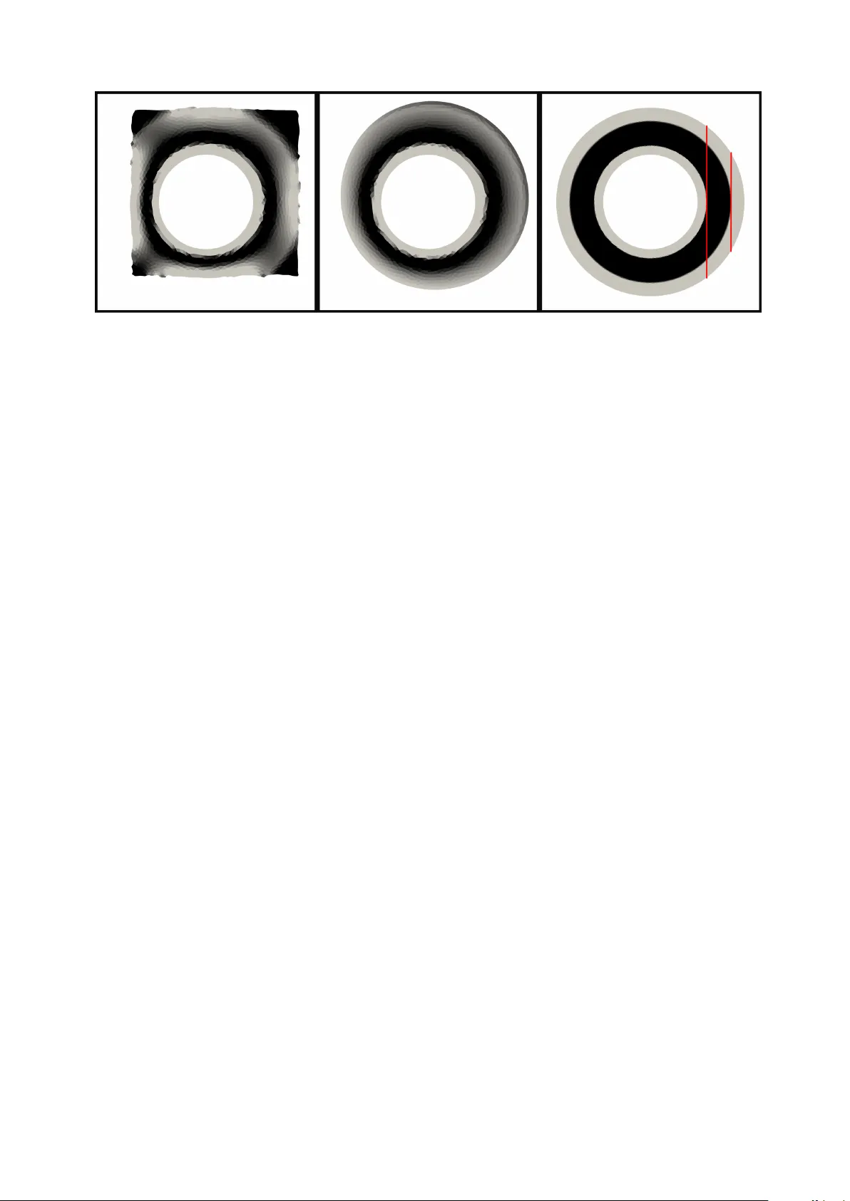
Authors: Marko Erceg, Petar Kunštek, Marko Vrdoljak
Hybrid Optimization T ec hniques for Multi-State Optimal Design Problems Mark o Erceg ∗ , P etar Kun ˇ stek † , Mark o V rdoljak ‡ Abstract This pap er addresses optimal design problems go v erned b y m ulti-state stationary diffusion equations, aiming at the sim ultaneous optimization of the domain shap e and the distribution of t w o isotropic materials in prescrib ed prop ortions. Existence of generalized solutions is established via a h ybrid approach combining homogenization- based relaxation in the in terior with suitable restrictions on admissible domains. Based on this framework, we prop ose a n umerical metho d that integrates homog- enization and shap e optimization. The domain b oundary is evolv ed using a level set metho d driven b y the shap e deriv ative, while the interior material distribution is up- dated via an optimalit y criteria algorithm. The approach is demonstrated on a repre- sen tativ e example. Keyw ords : optimal design, homogenization, optimalit y conditions, shap e deriv ativ e, Haus- dorff distance Mathematics Sub ject Classification 2010 : 49Q10, 49K20, 65N30, 80M50 1 In tro duction Shap e optimization refers to the determination of an optimal domain that minimizes a pre- scrib ed ob jectiv e functional, usually defined b y the solution of a partial differential equation (PDE) kno wn as the state equation. As suc h, shape optimization can be considered as a branc h of distributed con trol theory , where the domain acts as a control v ariable. A fundamen tal difficulty in this field lies in the nonexistence of classical optimal shap es. Minimizing sequences of domains tend to dev elop oscillations, holes, or degeneracies, so that no Lipschitz domain attains the infim um of the cost functional. This nonexistence has profound implications: n umerical algorithms may fail to con verge or dep end strongly on the initial guess. Tw o principal strategies hav e emerged to address this: (i) restricting the class of admissible domains to ensure compactness and existence, or (ii) relaxing the problem b y enlarging the admissible set where existence can b e reco vered. The homogenization theory pla ys a cen tral role in obtaining this relaxation [ 32 , 26 ], by in tro ducing a notion of generalized designs that ensures the optimization problem remains w ell-p osed and ph ysically meaningful. This, in turn, leads to more stable and efficient n umerical computations of relaxed designs [ 8 , 2 , 9 ]. ∗ Departmen t of Mathematics, F aculty of Science, Universit y of Zagreb, Croatia, maerceg@math.hr † Departmen t of Mathematics, F aculty of Science, Universit y of Zagreb, Croatia, petar@math.hr ‡ Departmen t of Mathematics, F aculty of Science, Universit y of Zagreb, Croatia, marko@math.hr 1 On the other hand, imp osing additional (uniform) regularity assumptions on the class of admissible domains can ensure the existence of solutions for certain shap e optimization problems. Examples include the uniform cone condition [ 16 , 35 ], a b ounded n umber of con- nected comp onents of the complemen t in t w o-dimensional cases [ 39 ], p erimeter constraints [ 6 ], uniform contin uit y conditions [ 29 ], the uniform cusp prop erty [ 18 ], and uniform b ound- edness of the densit y p erimeter [ 13 ]. F urther theoretical insigh ts are provided in [ 38 , 23 , 12 , 34 ]. This theoretical developmen t was accompanied b y a numerical treatment of the problem using shape calculus, building on the pioneering w ork of Hadamard [ 33 , 35 , 38 , 5 ]. Nu- merical metho ds in shap e optimization differ mainly in ho w they represen t geometry . Some approac hes, such as the level set and phase-field methods, describ e shap es implicitly using a scalar field that marks the region o ccupied by the material. Other approaches repre- sen t shap es explicitly through a computational mesh or CAD mo del, allo wing for accurate analysis but requiring frequen t remeshing or geometric up dates as the shap e evolv es. In this pap er, we consider the problem of determining not only the optimal distribution of tw o phases but also the optimal shap e of the region they o ccup y . The problem has b een addressed in the literature using alternativ e approac hes. Extensions of the SIMP scheme to m ultiple phases were prop osed in [ 37 , 19 ], considering three-phase mixtures (tw o materials plus void). In [ 45 , 4 ], the lev el set metho d w as applied to multi-phase shap e optimization, also allowing one of the phases to represent v oid. Motiv ated b y the robustness of the homogenization metho d, our approac h combines homogenization-based relaxation within the domain with shap e optimization based on the shap e deriv ative of the o verall region. F or this reason, w e refer to it as a h ybrid metho d. Moreo ver, the optimality criteria metho d is known to pro duce accurate approximations within only a few iterations, which facilitates the application of the shap e deriv ativ e metho d to the external b oundary . The resulting optimal design can, through p enalization techniques, b e reduced to a clas- sical design with pure phases, or it can serv e as an informed initial guess for the subsequen t application of the shap e deriv ativ e metho d to the distribution of the tw o phases within the “optimal” domain. In the n umerical example presen ted in the final section, the p enaliza- tion step was not implemen ted, since the optimal design pro duced b y the prop osed metho d turned out to b e classical. This is due to the radial symmetry of the problem: the resulting design is known to b e optimal for the fixed-domain problem p osed on the resulting domain [ 27 ]. W e now pro ceed to form ulate the sp ecific t wo-material optimal design problem under consideration. Let D ⊂ R d , d ≥ 2, be a b ounded op en fixed set and Ω ⊂ D a Lipschitz domain. The op en set Ω is made of tw o materials with isotropic conductivities 0 < α < β , so its o verall conductivit y is given by (1) A = χα I + (1 − χ ) β I , where χ ∈ L ∞ (Ω; { 0 , 1 } ) represents the c haracteristic function of the less-conductiv e phase. F or different right-hand sides f 1 , . . . f m ∈ L 2 ( D ) w e denote the corresp onding temp eratures u := ( u 1 , . . . , u m ) ∈ H 1 (Ω; R m ) of the b ody , as the unique solutions of the follo wing boundary 2 v alue problems (2) − div( A ∇ u i ) = f i in Ω u i = h i on Γ 0 u i = 0 on Γ 1 A ∇ u i · n = 0 on Γ 2 . Here, the b oundary ∂ Ω consists of three parts: ∂ Ω = Γ 0 ˙ ∪ Γ 1 ˙ ∪ Γ 2 , where Γ 0 is relatively op en and fixed, and h i ∈ H 1 2 (Γ 0 ) are prescrib ed. The sets Γ 1 and Γ 2 represen t subsets of D on whic h the Dirichlet and Neumann b oundary conditions, resp ectiv ely , can b e applied. Note that simply requiring h i ∈ H 1 2 (Γ 0 ) is insufficient to ensure well-posedness; their choice must b e consisten t with the other b oundary conditions, particularly the homogeneous Diric hlet condition imp osed on the segment Γ 1 . W e address this sp ecification separately within each of the three settings in Section 2 . Remark 1.1. The functions f i , for i = 1 , . . . , m , c ould p otential ly b elong to a br o ader sp ac e, sp e cific al ly the dual of the sp ac e v ∈ H 1 ( D ) : v | Γ 0 ∪ Γ 1 = 0 , wher e the r estriction is natur al ly understo o d in the sense of tr ac es. However, for the sake of simplicity in the subse quent analy- sis, and anticip ating the even stricter r e quir ements of the numeric al applic ation to fol low, we shal l work with a subsp ac e c onsisting of squar e inte gr able functions on D (i.e. f i ∈ L 2 ( D ) ). The aim is to find a domain Ω, suc h that Γ 0 ⊆ ∂ Ω, and a characteristic function χ that minimizes the ob jectiv e functional I (Ω , χ ) = Z Ω χ ( x ) g α ( x , u ( x )) + (1 − χ ( x )) g β ( x , u ( x )) d x . The amount of the first phase is also giv en: Z Ω χ d x = q α , as well as the v olume (i.e. the Leb esgue measure) of the domain: | Ω | = V . There is no definitiv e reason to e xp ect minimizers; ho wev er, if they do exist, w e refer to this as a classical design. W e provide a brief ov erview of the pap er. In Section 2 , we in tro duce a h ybrid approac h for establishing the existence of a (generalized) solution. Relaxation via the homogenization metho d is applied within the domain, while the class of admissible domains is suitably re- stricted. W e first examine the cases where either Γ 1 or Γ 2 is empty , and then extend the analysis to the general case b y combining the techniques dev elop ed for these tw o settings. Section 3 presen ts the numerical approac h corresp onding to this hybrid framework. The op- timalit y criteria metho d is applied inside the domain, while the domain b oundary is updated using the shap e deriv ative of the cost functional. Section 4 illustrates the approac h with a n umerical example. 2 Relaxation 2.1 Preparation If Ω is fixed, ac hieving prop er relaxation in v olves introducing generalized materials, which are mixtures of t w o original phases on a micro-scale, in tro duced by Murat and T artar [ 32 ]. 3 In this relaxation pro cess, characteristic functions χ ∈ L ∞ (Ω; { 0 , 1 } ) are replaced b y local fractions θ ∈ L ∞ (Ω; [0 , 1]), and ( 1 ) b y A ∈ K ( θ ) almost everywhere on Ω, where K ( θ ) denotes the set of all p ossible effective conductivities obtained by mixing original phases with local fraction θ . Under suitable growth conditions on g α and g β (see (A5) b elow) the relaxed problem reads (3) ( J (Ω , θ , A ) = R Ω θ ( x ) g α ( x , u ( x )) + (1 − θ ( x )) g β ( x , u ( x )) d x → min θ ∈ L ∞ (Ω; [0 , 1]) , R Ω θ d x = q α , A ∈ K ( θ ) a.e. in Ω , u solves ( 2 ) . The determination of the set K ( θ ) is reffered to as the G-closure problem (see [ 2 , Sub- section 2.1.2]). F or mixtures of tw o isotropic phases, this problem admits a complete char- acterization: K ( θ ) consists of all symmetric matrices whose eigenv alues satisfy the following inequalities (see [ 32 , 30 ]) (4) λ − θ ≤ λ j ≤ λ + θ j = 1 , . . . , d d X j =1 1 λ j − α ≤ 1 λ − θ − α + d − 1 λ + θ − α d X j =1 1 β − λ j ≤ 1 β − λ − θ + d − 1 β − λ + θ where λ − θ = ( θ /α + (1 − θ ) /β ) − 1 , λ + θ = θ α + (1 − θ ) β . This precise characterization of K ( θ ) is relev an t only for the numerical approac h and is not required for the results presen ted in this section. These results equally apply to the case of mixing more than t wo materials, including anisotropic ones [ 42 , 41 ]. T o obtain existence of optimal Ω, w e shrink the set of admissible domains, b y assuming the well-kno wn cone condition. F or y , ξ ∈ R d , ξ a unit vector, and ε > 0 we denote b y C ( y , ξ , ε ) the cone of vertex y , of direction ξ and dimension ε , i.e. (5) C ( y , ξ , ε ) = z ∈ R d : ( z − y ) · ξ ≥ | z − y | cos ε, 0 < | z − y | < ε . An op en set Ω is said to hav e ε -c one pr op erty if (v. Figure 1 ) ( ∀ x ∈ ∂ Ω)( ∃ ξ x ∈ R d , | ξ x | = 1)( ∀ y ∈ Ω ∩ B ( x , ε )) C ( y , ξ x , ε ) ⊂ Ω . Here B ( x , ε ) denotes the op en ball cen tred at x with radius ε , while Ω stands for the closure of the set Ω. This prop erty , when considered for a single domain Ω, is commonly referred to as the uniform cone prop ert y [ 20 ]. How ever, in problems inv olving a family of domains Ω, emphasizing the uniformity of the parameter ε across the en tire family is crucial, whic h mak es the term ε -cone prop erty w ell-established [ 23 ]. It is a well-kno wn result that the ε -cone prop erty is equiv alen t to the (uniform) Lipschitz condition on the b oundary of the domains [ 16 ] (see also [ 23 , Theorem 2.4.7]). Let us now introduce the set of relaxed admissible designs. W e b egin b y addressing the standing assumptions that are required to define these designs. F or the reader’s con v enience, w e will also use the con text of these assumptions to fix and define some notation that will b e used throughout the pap er. 4 Figure 1: The ε -cone property of a set (A1) D ⊂ R d is an op en and b ounded set (reference domain), where d ≥ 2 is a fixed in teger. (A2) 0 < α < β (material conductivities), V > 0 (volume constraint), q α ∈ (0 , V ) (quantit y of the first phase), ε > 0 (regularit y of domains) are fixed. (A3) Let M ⊂ D b e a fixed, compact ( d − 1)-dimensional Lipsc hitz manifold with b oundary . W e define Γ 0 as the manifold interior of M , namely Γ 0 = M \ ∂ M , where ∂ M denotes the manifold boundary of M . Then, the set Γ 0 admits a finite decomp osition in to connected comp onents Γ i 0 , i = 1 , 2 , . . . , N , whose closures are m utually disjoin t: for any i, j ∈ { 1 , 2 , . . . , N } , i = j , w e ha v e Γ i 0 ∩ Γ j 0 = ∅ . In particular, each Γ i 0 is an op en ( d − 1)-dimensional Lipschitz manifold whose b oundary ∂ Γ i 0 = Γ i 0 \ Γ i 0 consists precisely of those p oin ts at which the comp onen t meets the manifold b oundary ∂ M . (A4) There exists an op en and connected b Ω ⊆ D satisfying the ε -cone prop erty , | b Ω | = V , and Γ 0 ⊆ ∂ b Ω, where | b Ω | represents the Leb esgue measure of the set b Ω. The admissible set, i.e. the set of admissible designs , is then defined as (6) A = ( (Ω , θ , A ) : Ω ⊆ D is op en, connected and satisfies the ε -cone prop erty , | Ω | = V , Γ 0 ⊂ ∂ Ω , θ ∈ L ∞ (Ω; [0 , 1]) , Z Ω θ d x = q α , A ∈ K ( θ ) a.e. in Ω ) . The set A dep ends on all parameters in tro duced in (A1)–(A3), but for simplicity we shall not include that explicit dependence in the notation. Note that b y (A4) the set of admissible designs A is non-empt y . Indeed, ( b Ω , χ, A ), with characteristic function χ on b Ω satisfying constrain t on the amoun t of the first phase, and A giv en b y ( 1 ) b elongs to A . Let O denote the pro jection on to the first comp onen t of A , i.e. Ω ∈ O if and only if there exist θ and A suc h that (Ω , θ , A ) ∈ A . The elements of O will b e referred to as admissible domains . 5 The relaxed optimal design problem can b e stated as follows: (7) ( J (Ω , θ , A ) → min (Ω , θ , A ) ∈ A , and u solves ( 2 ) with A . The functions g α and g β are sub ject to the follo wing assumptions. (A5) g α , g β are Carath ´ eo dory functions on D × R m (measurable in x for every u , and con- tin uous in u for almost every x ) satisfying the gro wth condition | g γ ( x , u ) | ≤ ϕ γ ( x ) + ψ γ ( x ) | u | q , γ = α, β , for some q ∈ [1 , q ∗ ⟩ and ϕ γ ∈ L s 1 ( D ), ψ γ ∈ L s 2 ( D ), where s 1 > 1 and q ∗ = + ∞ , d = 2 2 d d − 2 , d > 2 , s 2 > 1 , d = 2 q ∗ q ∗ − q , d > 2 . In the rest of this section, we prov e the existence of a solution to the relaxed problem ( 7 ), under a suitable assumption on h i . The analysis is structured in to three steps related to the b oundary conditions of the state problem, as defined by the b oundary decomp osition in ( 2 ). W e first study the pure Diric hlet problem, where Γ 2 = ∅ , then we examine the mixed problem with a fixed Dirichlet part, where Γ 1 = ∅ , and as a final step, we address the general setting, whic h cov ers b oth previously addressed cases. W e presen t these three distinct settings sequentially to enhance accessibilit y and guide the reader step-b y-step through the tec hnical difficulties. This approac h keeps the pro ofs reasonably short, as in the second and third cases, we emphasize only the new technical comp onents without rep eating the parts that carry o ver from the preceding analysis. A final tec hnical result in this section concerns the geometry of Γ 0 . Lemma 2.1. L et us assume (A1) – (A4) . Ther e exist N op en and b ounde d disjoint subsets O i ⊂ R d , i = 1 , 2 , . . . , N , such that for every i ∈ { 1 , 2 , . . . , N } the fol lowing hold: i) Γ i 0 ⊂ O i and ∂ Γ i 0 ⊂ ∂ O i ; ii) O i = O i − ˙ ∪ Γ i 0 ˙ ∪ O i + , wher e O i ± ar e c onne cte d op en sets; iii) The b oundary of any admissible domain Ω ∈ O satisfies ∂ Ω ∩ O i = Γ i 0 , wher e O is the set of admissible domains define d in the ab ove. Pr o of. By [ 16 ] (see also [ 23 , Theorem 2.4.7]) any admissible domain Ω ∈ O has a Lipsc hitz b oundary . More precisely , in terms of [ 23 , Definition 2.4.5], the parameters in the definition of a Lipsc hitz b oundary are L, a, r ∈ (0 , ∞ ), and they dep end only on ε . W e define δ = δ ( ε ) := min { r , a, 1 } √ 1 + L 2 . Let us tak e an arbitrary i ∈ { 1 , 2 . . . , N } . Then we define O i := [ x ∈ Γ i 0 B ( x, η x ) , 6 where η x = δ min { 1 , d ( ∂ Γ i 0 , x ) } . Then clearly we ha ve that O i is op en and that i) is satisfied. Using the definition of a Lipschitz b oundary [ 23 , Definition 2.4.5] it is easy to sho w that for an y admissible domain Ω ∈ O we hav e ∂ Ω ∩ B ( x, η x ) = Γ i 0 ∩ B ( x, η x ) (here the c hoice of δ is fundamen tal). This immediately implies that iii) is fulfilled. This completes the pro of. An immediate consequence of the previous lemma is that Γ 0 is relativ ely op en in ∂ Ω for an y admissible domain Ω ∈ O . Remark 2.2. The interpr etation of the op en set O := ∪ N i =1 O i is that the b oundary of al l admissible domains Ω ∈ O is fixe d within O . Henc e, ∂ Ω \ Γ 0 is c ontaine d in D \ O . One c ould imp ose such a c ondition in the definition of O , but the pr evious lemma pr e cisely asserts that this is implicitly implie d by the existing assumptions and is ther efor e not r e quir e d as an a priori c ondition. However, we c annot claim that the entir e admissible domain Ω is fixe d within O . Inste ad, for any given i ∈ { 1 , 2 , . . . , N } , the domain Ω interse cts O i in one of two sp e cific ways: Ω ∩ O i = O i − or Ω ∩ O i = O i + . We also al low the fixe d b oundary to interse ct the exterior b oundary of D , i.e. Γ 0 ∩ ∂ D = ∅ . Then, some sets O i ar e not strictly c ontaine d in D ( O i ⊆ D ), so that, of the two e qualities ab ove, only one holds, and it is the same for every Ω ∈ O . 2.2 Diric hlet-t yp e free b oundary Let us start b y imp osing the condition on functions h i . (H1) F or any i ∈ { 1 , 2 , . . . , m } there exists H i ∈ H 1 0 ( O ) such that h i = H i | Γ 0 , where O = ∪ N j =1 O j , and O j are given by Lemma 2.1 . W e obtain the follo wing existence result. Theorem 2.3. Under assumptions (A1) – (A5) and (H1) , the optimal design pr oblem ( 7 ) admits a solution in the c ase Γ 2 = ∅ . Pr o of. Step I. Let (Ω n , θ n , A n ) be a minimizing sequence asso ciated to ( 7 ). Our aim is to find a conv ergen t subsequence (in the righ t sense) and pro v e that the limit solv es the problem. W e b egin by analyzing the sequence (Ω n ). By [ 23 , Theorem 2.4.10], see also [ 16 ], there exists a subsequence of (Ω n ) (for simplicity of notation, w e do not relab el it), together with an op en Ω ⊆ D satisfying the ε -cone prop erty suc h that Ω n con verges to Ω in the sense of Hausdorff for op en sets, in the sense of characteristic functions and in the sense of compacts (for precise definitions, see [ 23 , Section 2.2]). Moreov er, b oth Ω n and ∂ Ω n con verge in the Hausdorff sense for compact sets to Ω and ∂ Ω, resp ectively (cf. [ 25 ]). Our goal is to sho w that the limit set Ω b elongs to O . Since all Ω n are connected, the same holds for the sequence of closures Ω n . Hence, it follo ws by [ 23 , Prop osition 2.2.19] that the limit set Ω is also connected. Consequen tly , since Ω is a Lipsc hitz domain, it is connected as w ell. The con vergence in the sense of c haracteristic functions implies that the volume is preserved, i.e. | Ω | = ∥ χ Ω ∥ L 1 ( D ) = lim n ∥ χ Ω n ∥ L 1 ( D ) = lim n | Ω n | = V . 7 Th us, it is left to c hec k that Γ 0 ⊆ ∂ Ω. This follo ws immediately from Γ 0 ⊆ ∂ Ω n and ∂ Ω n → ∂ Ω in the sense of Hausdorff (see [ 23 , Subsection 2.2.3.2]). Let us no w fo cus on ( θ n ). W e first extend eac h θ n b y zero to the whole D and w e denote this extension by ˜ θ n . Then w e obviously ha v e ˜ θ n ∈ L ∞ ( D ; [0 , 1]). Hence, we can pass to a subsequence (again not relab eled) suc h that ˜ θ n con verges weakly- ∗ to ˜ θ ∈ L ∞ ( D ; [0 , 1]). Let us denote θ := ˜ θ | Ω . Then θ ∈ L ∞ (Ω; [0 , 1]) and Z Ω θ ( x ) d x = Z D χ Ω ( x ) ˜ θ ( x ) d x = lim n Z D χ Ω n ( x ) ˜ θ n ( x ) d x = lim n Z Ω n θ n ( x ) d x = q α . It remains to analyze the sequence ( A n ). F or ev ery n ∈ N , w e hav e A n ∈ K ( θ n ) almost ev erywhere on Ω n . Our aim is to extend A n to the whole domain D , denoting the extension b y e A n , in suc h a wa y that the preceding prop erty remains v alid when A n , θ n and Ω n are replaced by e A n , ˜ θ n and D , resp ectiv ely: e A n ( x ) := A n ( x ) , x ∈ Ω n β I , x ∈ D \ Ω n . No w w e can apply compactness of the H-conv ergence (see [ 2 , subsections 1.2.4 and 2.1.2] and [ 40 , Chapter 6]), which ensures existence of e A ∈ K ( ˜ θ ) and a subsequence (not relabeled) suc h that ( e A n ) H-conv erges to e A . Hence, for A := e A | Ω , by the previous analysis, w e ha ve (Ω , θ , A ) ∈ A , i.e. on the limit we got an admissible design. Step I I. T o write do wn weak form ulation of the b oundary v alue problem (8) − div( A n ∇ u n i ) = f i in Ω n u n i = h i on Γ 0 u n i = 0 on Γ n 1 , w e b egin by homogenizing the b oundary conditions on Γ 0 . W e use the same notation for the extension by zero to the whole R d of H i giv en in (H1). It is w ell-known that H i ∈ H 1 ( R d ) (see [ 1 , Lemma 3.27]). Defining v n i = u n i − H i | Ω n , for i = 1 , 2 , . . . , m , w e see that v n i is the unique solution of (9) − div( A n ∇ v n i ) = f i + g n i in Ω n v n i = 0 on ∂ Ω n = Γ 0 ∪ Γ n 1 , where g n i := div A n ∇ ( H i | Ω n ) ∈ H − 1 (Ω n ). This step relies on the conditions H i | Γ 0 = h i and H i | Γ n 1 = 0 for all n ∈ N (cf. (H1) and Lemma 2.1 (iii)). Applying A n ∈ K ( θ n ), we hav e ∥ g n i ∥ H − 1 (Ω n ) ≤ β ∥ H i ∥ H 1 (Ω n ) ≤ β ∥ H i ∥ H 1 ( R d ) = β ∥ H i ∥ H 1 ( O ) , where we hav e used that supp H i ⊆ O . Let us denote by e v n the extension of v n = ( v n 1 , . . . , v n m ) b y zero on D \ Ω n . Then e v n ∈ H 1 0 ( D ; R m ). Moreo ver, using the a priori estimate, w e ha v e that ( e v n ) is bounded in H 1 0 ( D ; R m ) (cf. [ 23 , Proposition 3.2.1]). Indeed, for any i ∈ { 1 , 2 , . . . , m } and any n ∈ N w e ha v e (10) αc 1 ∥ e v n i ∥ 2 H 1 0 ( D ) ≤ α Z D |∇ e v n i | 2 = α Z Ω n |∇ v n i | 2 ≤ Z Ω n A n ∇ v n i · ∇ v n i = ⟨ f n i , v n i ⟩ H − 1 (Ω n ) , H 1 0 (Ω n ) ≤ c 2 ∥ v n i ∥ H 1 0 (Ω n ) = c 2 ∥ e v n i ∥ H 1 0 ( D ) , 8 where the P oincar´ e inequalit y (the constant c 1 dep ends only on the set D ; see [ 1 , Corollary 6.31]) is applied first. In the second step we hav e used that ∇ e v n i agrees with the zero extension of ∇ v n i (cf. [ 1 , Lemma 3.27]). Then the co ercivity of A n is used, the weak form ulation of ( 9 ), and the b oundedness of f n i := f i | Ω n + g n i in H − 1 (Ω n ) ( c 2 b eing max i ( ∥ f i ∥ L 2 ( D ) + β ∥ H i ∥ H 1 ( O ) )). Therefore, w e can pass to another subsequence suc h that ( e v n ) is w eakly conv ergen t to e v in H 1 0 ( D ; R m ) and conv erges almost everywhere on D (for the latter we use that by the Rellich- Kondra ˇ sov compactness theorem ( e v n ) con verges strongly in L 2 ( D ; R m ); see [ 1 , Corollary 2.17 and Theorem 6.3]). Finally , e u n := e v n + H con v erges to e u := e v + H weakly in H 1 ( D ; R m ) and almost ev erywhere, as well (here H = ( H 1 , . . . , H m )). Let us in tro duce v := e v | Ω and u := e u | Ω . W e w an t to sho w that u is a unique solution of ( 2 ), where A and Ω are previously defined. Step I I I. F or any n ∈ N we hav e 0 = ( χ D − χ Ω n ) e v n a.e. in D . P assing to the limit (p ossibly on a subsequence to ensure that ( χ Ω n ) conv erges a.e. to χ Ω ) we obtain that e v = 0 a.e. on D \ Ω. Hence, v ∈ H 1 0 (Ω; R m ) (see e.g. [ 23 , Prop osition 3.2.16]). Let us take an arbitrary i ∈ { 1 , 2 , . . . , m } . It remains to sho w that u i = v i + H i | Ω , satisfies the w eak form ulation asso ciated with ( 2 ). By rev ersing the ab ov e procedure of homogenizing the b oundary conditions on Γ 0 , it is eviden t that it is sufficien t to obtain that v i is a weak solution to ( 9 ) with Ω n , A n and g n i replaced by Ω, A and g i := div A ∇ ( H i | Ω ), respectively . Note that g i satisfies the same b ound as g n i . Fix an arbitrary test function ϕ ∈ C ∞ c (Ω). Giv en this test function ϕ , select an op en set U suc h that supp ϕ ⊆ U ⊂ ⊂ Ω. Since (Ω n ) conv erges to Ω in the sense of compacts (cf. [ 23 , Prop osition 2.2.17]), there exists n 1 = n 1 ( U ) ∈ N such that for an y n ≥ n 1 w e ha ve U ⊂ ⊂ Ω n . In particular, ϕ ∈ C ∞ c (Ω n ). Th us, ϕ is an admissible test function for the w eak form ulation of the problem for v n i , i.e. for an y n ≥ n 1 w e ha v e Z Ω n A n ∇ v n i · ∇ ϕ d x = ⟨ f i | Ω n + g n i , ϕ ⟩ H − 1 (Ω n ) , H 1 0 (Ω n ) . By moving ⟨ g n i , ϕ ⟩ H − 1 (Ω n ) , H 1 0 (Ω n ) = − R Ω n A n ∇ ( H i | Ω n ) · ∇ ϕ d x to the left-hand side we get u n i in place of v n i . Moreo ver, using that f i ∈ L 2 ( D ) and supp ϕ ⊆ U ⊂ ⊂ Ω ∩ Ω n , we hav e ⟨ f i | Ω n , ϕ ⟩ H − 1 (Ω n ) , H 1 0 (Ω n ) = Z U f i ( x ) ϕ ( x ) d x . Th us, the following holds: (11) Z U A n ∇ u n i · ∇ ϕ d x = Z U f i ( x ) ϕ ( x ) d x , where we accounted for the fact that ϕ ∈ C ∞ c ( U ). It remains to analyse the limit of the left-hand side in ( 11 ). More precisely , w e wan t to sho w that it conv erges, as n tends to infinit y , to R U A ∇ u i · ∇ ϕ d x . Here, we utilize the concept of H-con v ergence to study the b ehavior of the term A n ∇ u n i , with the aim of applying [ 2 , Prop osition 1.2.19] (see also [ 40 , Lemma 13.2]). Let us start by noting that, as shown in [ 40 , Lemma 10.5], A n | U = e A n | U H-con verges to A | U = e A | U (recall that n ≥ n 1 ). F urthermore, since ( 11 ) holds for an y ϕ ∈ C ∞ c ( U ), w e hav e that − div A n | U ∇ ( u n i ) | U = f i | U ∈ L 2 ( U ) . 9 Therefore, since u n i | U u i | U w eakly in H 1 ( U ), w e may apply [ 2 , Prop osition 1.2.19], which yields A n | U ∇ ( u n i ) | U A | U ∇ ( u i ) | U w eakly in L 2 loc ( U ; R d ). Returning to the left-hand side of ( 11 ) w e get lim n →∞ Z U A n ∇ u n i · ∇ ϕ d x = Z U A ∇ u i · ∇ ϕ d x = Z Ω A ∇ v i · ∇ ϕ d x − ⟨ g i , ϕ ⟩ H − 1 (Ω) , H 1 0 (Ω) . Finally , by the arbitrariness of ϕ and the density of C ∞ c (Ω) in H 1 0 (Ω), the function v i is the weak solution of ( 9 ), with Ω n , A n and g n i replaced by Ω, A and g i , resp ectively . In ligh t of the preceding observ ations, this immediately leads the desired conclusion that u i is the w eak solution to ( 2 ). Step IV. The final task is to prov e that J (Ω n , θ n , A n ) conv erges to J (Ω , θ , A ), i.e. that the relaxed admissible design (Ω , θ , A ) is the minimizer of J on A . The v alue of the functional J at the design configuration (Ω n , θ n , A n ) can b e expressed as (note that here we w ork with the final subsequence obtained in the previous step): J (Ω n , θ n , A n ) = Z D χ Ω n ( x ) ˜ θ n ( x ) g α ( x , e u n ( x )) + (1 − ˜ θ n ( x )) g β ( x , e u n ( x )) d x . This represen tation is useful for clearly separating the ingredients that are already under con trol from those that still require justification in order to pass to the limit as n tends to infinit y . Indeed, χ Ω n strongly con verges to χ Ω in an y L s ( D ), s ∈ [1 , ∞⟩ (since (Ω n ) con verges to Ω in the sense of characteristic functions; cf. [ 23 , Definition 2.2.3]), while ( ˜ θ n ) con v erges w eakly- ∗ to ˜ θ in L ∞ ( D ). Consequen tly , it suffices to prov e that there exists p > 1 such that g γ ( · , e u n ) conv erges strongly to g γ ( · , e u ) in L p ( D ), γ ∈ { α, β } . Since e u n ( x ) con verges to e u ( x ) for a.e. x ∈ D and g γ , γ ∈ { α, β } , are Carath ´ eo dory functions on D × R m , we hav e that g γ ( x , e u n ( x )) n →∞ − → g γ ( x , e u ( x )) a.e. x ∈ D , γ ∈ { α , β } . In order to conclude the argumen t via the Leb esgue dominated conv ergence theorem, it remains to find, for some p > 1, an L p -in tegrable function that serv es as a dominating function for | g γ ( · , e u n ) | . A more precise application of the Rellic h-Kondra ˇ sov theorem (see [ 1 , Theorem 6.3]) implies that, for an y r ∈ [1 , q ∗ ⟩ , the sequence ( e u n ) con v erges strongly to e u in L r ( D ), where q ∗ is defined in (A5). Hence, for an y r ∈ [1 , q ∗ ⟩ there exists w ∈ L r ( D ) suc h that | e u n ( x ) | ≤ w ( x ) a.e. x ∈ D . Then from the gro wth condition on g γ w e get | g γ ( x , e u n ( x )) | ≤ | ϕ γ ( x ) | + | ψ γ ( x ) | w ( x ) q =: G ( x ) , a.e. x ∈ D . No w w q ∈ L r q ( D ) and b y the H¨ older inequality ψ γ w q b elongs to L s ( D ) with s > 1 if 1 s := 1 s 2 + q r < 1 , where we hav e the freedom to choose the v alue r ∈ [1 , q ∗ ⟩ . F or d = 2 b y (A5) w e ha v e 1 s 2 < 1, and since q ∗ = ∞ , the parameter r can b e c hosen so that q r is arbitrarily small. On the other hand, for d > 2 it suffices that 1 s 2 + q q ∗ < 1 b ecause r can b e taken arbitrarily close to q ∗ . Hence the assumption (A5) ensures that these conditions are satisfied. Therefore, G ∈ L p ( D ), with p = min { s 1 , s } > 1. This completes the pro of. 10 Remark 2.4. The r esult of The or em 2.3 stil l holds if we r emove assumption (A3) and set Γ 0 = ∅ . However, fr om the p ersp e ctive of c oncr ete applic ations, this sc enario is not of p articular imp ortanc e, as the p osition of the admissible sets is typic al ly fixed using the fixe d p ortion of the b oundary Γ 0 . 2.3 Neumann-t yp e free b oundary T o b egin with, we consider the case in whic h the entire free part of the b oundary is sub ject to a homogeneous Neumann b oundary condition, that is Γ 1 = ∅ . W e impose the following assumption on the functions h i : (H2) F or each i ∈ { 1 , 2 , . . . , m } there exists H i ∈ H 1 ( D ) such that h i = H i | Γ 0 . By (A3) w e kno w that the manifold b oundary of M , ∂ M , is a compact ( d − 2)-dimensional Lipsc hitz manifold (without boundary). Hence, ∂ M is locally the graph of a Lipschitz- con tinuous function and has a finite num b er of connected components. This is important since for any admissible domain Ω ∈ O w e hav e Γ 0 ∩ Γ 2 = ∂ M , where Γ 2 = ∂ Ω \ Γ 0 . Hence, the set of all smo oth functions ϕ ∈ C ∞ ( D ) that v anish on a neighborho o d of Γ 0 , when restricted to Ω, is dense in (12) V := { v ∈ H 1 (Ω) : v | Γ 0 = 0 } (see [ 10 , 11 ]). W e are now prepared to state and prov e the follo wing theorem. Theorem 2.5. Under assumptions (A1) – (A5) and (H2) , ther e exists a solution to the opti- mal design pr oblem ( 7 ) when Γ 1 = ∅ . Pr o of. F ollo wing the strategy used in the pro of of Theorem 2.3 , we shall highligh t only the steps where notew orthy differences are present. As in the pro of of Theorem 2.3 , w e b egin with a minimizing sequence (Ω n , θ n , A n ), and Step I from the previous pro of applies unchanged. The follo wing t wo steps requires greater care. Let us start with the analysis of the b oundary v alue problem (Step I I in the pro of of Theorem 2.3 ). F or any i ∈ { 1 , 2 , . . . , m } and any n ∈ N , there is a unique solution v n i to the follo wing v ariational problem: (13) Z Ω n A n ∇ ( v n i + H i ) · ∇ ϕ d x = Z Ω n f i ϕ d x , ϕ ∈ V n , where H i is given in (H2) and V n := { v ∈ H 1 (Ω n ) : v | Γ 0 = 0 } . Then it is easy to c heck that u n i = H i | Ω n + v n i ∈ H i | Ω n + V n is the unique w eak solution to (14) − div( A n ∇ u n i ) = f i in Ω n u n i = h i on Γ 0 A ∇ u n i · n = 0 on Γ n 2 = ∂ Ω n \ Γ 0 . In contrast to the previous pro of, w e mak e use of the extension e v n to the set D constructed according to the metho d presen ted b y Chenais [ 16 ]. Due to the uniform cone condition, there exists a constan t c 0 > 0, not dep ending on n such that (15) ∥ e v n i ∥ 2 H 1 ( D ) ≤ c 0 ∥ v n i ∥ 2 H 1 (Ω n ) . 11 Another crucial step is the usage of the P oincar ´ e inequalit y . While in the previous theorem the situation w as trivial (it w as applied on the space H 1 0 ( D )), here the existence of the uniform estimate for the extensions ensures that the constant in the Poincar ´ e inequalit y do es not dep end on n (see Lemma 2.6 b elo w). Thus, if we denote the constant by √ c 1 , w e ha ve (16) αc 1 ∥ e v n i ∥ 2 H 1 ( D ) ≤ αc 1 c 0 ∥ v n i ∥ 2 H 1 (Ω n ) ≤ c 0 Z Ω n A n ∇ v n i · ∇ v n i d x = c 0 Z Ω n f i v n i − A n ∇ H i · ∇ v n i d x ≤ c 0 ∥ f i ∥ L 2 ( D ) ∥ e v n i ∥ L 2 ( D ) + c 0 β ∥∇ H i ∥ L 2 ( D ; R d ) ∥∇ e v n i ∥ L 2 ( D ; R d ) ≤ c 2 ∥ e v n i ∥ H 1 ( D ) , where c 2 do es not dep end on n . Hence, the b oundedness of the sequence ( e v n ) in H 1 ( D ; R m ) follo ws. Therefore, now w e can easily adapt Step II of the previous pro of and obtain its w eak limit e v ∈ H 1 ( D ; R m ) (at a subsequence), and denote v := e v | Ω ∈ H 1 (Ω; R m ). Since the trace op erator is linear and contin uous, it follows that v = 0 on Γ 0 , i.e. each comp onen t of v b elongs to V (see ( 12 )). A t the same subsequence we ha ve weak con vergence of e u n := e v n + H to e u := e v + H , and in the same manner we denote u := e u | Ω , b elonging to the desired space H + V m . The next step is to pass to the limit in ( 13 ) (and then also in ( 14 )), whic h is more delicate when compared to the pro cedure used in the previous theorem. F or η > 0 w e in tro duce ω η = { x ∈ Ω : d ( x ; ∂ Ω) ≥ η } Γ η = { x ∈ R d : d ( x ; ∂ Ω) < η } . The compact set ω η is included in Ω b y definition, and for any p ositiv e η w e hav e Ω ⊆ Γ η ˙ ∪ ω η . Therefore, since (Ω n ) conv erges to Ω in the sense of compacts, for n large enough w e ha v e ω η ⊂ ⊂ Ω n Ω n ⊆ (Γ η ˙ ∪ ω η ) ∩ D = (Γ η ∩ D ) ˙ ∪ ω η , where we in addition used that Ω n ⊆ D . W e aim to pass to the limit in the equality ( 13 ), which can b e equiv alen tly rewritten as follo ws: (17) Z D χ Ω n e A n ∇ e u n i · ∇ ϕ d x = Z D χ Ω n f i ϕ d x , for any ϕ ∈ C ∞ ( D ) that v anish on a neigh b orho o d of Γ 0 . Here we make use of the fact that the set of all such functions, when restricted to Ω n is dense in V n [ 10 , Theorem 3.1]. The righ t-hand side of the previous equalit y con verges to R D χ Ω f ϕ i d x , since Ω n con verges to Ω in the sense of characteristic functions. F urthermore, the in tegral on the left-hand side of ( 17 ) is the sum of the same in te- grands o ver ω η and Γ η ∩ D . Again b y [ 2 , Proposition 1.2.19] w e hav e the con vergence A n | ω η ∇ ( u n i ) | ω η A | ω η ∇ ( u i ) | ω η w eakly in L 2 ( ω η ; R d ) which implies the conv ergence Z ω η χ Ω n A n ∇ u n i · ∇ ϕ d x = Z ω η A n ∇ u n i · ∇ ϕ d x → Z ω η A ∇ u i · ∇ ϕ d x = Z ω η χ Ω A ∇ u i · ∇ ϕ d x . 12 Finally , for the in tegral o ver Γ η w e ha v e Z Γ η ∩ D χ Ω n e A n ∇ e u n i · ∇ ϕ d x − Z Γ η ∩ D χ Ω e A ∇ e u i · ∇ ϕ d x ≤ Z Γ η ∩ D | e A n ∇ e u n i · ∇ ϕ | d x + Z Γ η ∩ D | e A ∇ e u i · ∇ ϕ | d x ≤ ∥ e A n ∇ e u n i ∥ L 2 ( D ; R d ) ∥∇ ϕ ∥ L 2 (Γ η ∩ D ; R d ) + ∥ e A ∇ e u i ∥ L 2 ( D ; R d ) ∥∇ ϕ ∥ L 2 (Γ η ∩ D ; R d ) ≤ β ∥∇ ϕ ∥ L ∞ ( D ; R d ) ∥ e u n i ∥ H 1 ( D ) + ∥ e u i ∥ H 1 ( D ) q | Γ η ∩ D | ≤ c q | Γ η | , where constant c do es not dep end on n . Since | Γ η | conv erges to zero as η go es to zero, w e can pass to the limit in ( 17 ) and conclude Z Ω A ∇ u i · ∇ ϕ d x = Z Ω f i ϕ d x , i = 1 , . . . , m , for an y ϕ ∈ C ∞ ( D ) that v anish on a neighborho o d of Γ 0 , which means that the limit u solv es ( 2 ). Finally , w e apply Step IV of the previous pro of directly , whic h completes the pro of. Here we pro vide an imp ortant uniform Poincar ´ e inequalit y for admissible domains. The strategy of the pro of is standard and relies on Chenais’s extension (see e.g. [ 22 , Lemma 2.19]); how ev er, for completeness, w e provide the full pro of. Lemma 2.6. Ther e exists a c onstant c > 0 such that for any admissible domain Ω ∈ O and u ∈ V = { v ∈ H 1 (Ω) : v | Γ 0 = 0 } it holds c ∥ u ∥ H 1 (Ω) ≤ ∥∇ u ∥ L 2 (Ω; R d ) . Pr o of. Let us assume that the claim do es not hold. Then for any n ∈ N there exist Ω n ∈ O and u n ∈ V n = { v ∈ H 1 (Ω n ) : v | Γ 0 = 0 } such that ∥ u n ∥ L 2 (Ω n ) = 1 and 1 n ∥ u n ∥ H 1 (Ω n ) > ∥∇ u n ∥ L 2 (Ω n ; R d ) . Hence, since ∥ u n ∥ 2 H 1 (Ω n ) = 1 + ∥∇ u n ∥ 2 L 2 (Ω n ; R d ) , w e get ∥∇ u n ∥ L 2 (Ω n ; R d ) < 1 √ n 2 − 1 , n ≥ 2, implying lim n →∞ ∥∇ u n ∥ L 2 (Ω n ; R d ) = 0 . In particular, the sequence of real num b ers ( ∥ u n ∥ H 1 (Ω n ) ) is bounded. Let us denote by e u n the extension of u n follo wing the metho d presented by Chenais [ 16 ]. Due to the uniform cone condition, there exists a constan t c 0 > 0 indep endent of n such that ∥ e u n ∥ H 1 ( D ) ≤ c 0 ∥ u n ∥ H 1 (Ω n ) , n ∈ N . Th us, ( e u n ) is b ounded in H 1 ( D ). Let us pass to a subsequence (keeping the same notation) suc h that ( e u n ) conv erges to v w eakly in H 1 ( D ) and strongly in L q ( D ) for an y q ∈ [1 , q ∗ ) (see [ 1 , Theorem 6.3]), where q ∗ is defined in (A5). 13 According to [ 23 , Theorem 2.4.10] (see also [ 16 ]), we can pass to another subsequence suc h that Ω n con verges to Ω ∈ O in the sense of Hausdorff (for op en sets) and in the sense of characteristic functions. Let us tak e an arbitrary ϕ ∈ C ∞ c ( D ). Using the Cauch y-Sc h w arz inequalit y , it holds Z Ω n ϕ ( x ) ∇ u n ( x ) d x ≤ ∥∇ u n ∥ L 2 (Ω n ; R d ) ∥ ϕ ∥ L 2 ( D ) n →∞ − − − → 0 . On the other hand, since ( χ Ω n ) con verges strongly to χ Ω in L 2 ( D ) and ( ∇ e u n ) con verges w eakly to ∇ v in L 2 ( D ; R d ), we hav e 0 = lim n Z Ω n ϕ ( x ) ∇ u n ( x ) d x = lim n Z D ϕ ( x ) χ Ω n ( x ) ∇ e u n ( x ) d x = Z D ϕ ( x ) χ Ω ( x ) ∇ v ( x ) d x = Z Ω ϕ ( x ) ∇ v ( x ) d x . Since ϕ ∈ C ∞ c ( D ) w as arbitrary , we get that ∇ v = 0 a.e. in Ω. Thus, v is a constant function on Ω (recall that Ω is connected). F urther on, since the trace is w eakly sequentially contin uous, from e u n | Γ 0 = u n | Γ 0 = 0, follo ws v | Γ 0 = 0. Th us, v = 0 a.e. in Ω. Ho wev er, since ( e u 2 n ) conv erges strongly in L p ( D ) for some p > 1 (in fact, p is any num b er in the in terv al (1 , q ∗ 2 )) and ( χ Ω n ) conv erges strongly in L r ( D ) for any r ∈ [1 , ∞ ), we can pass to the limit: 1 = ∥ u n ∥ 2 L 2 (Ω n ) = Z D χ Ω n ( x ) e u n ( x ) 2 d x n →∞ − − − → Z Ω v ( x ) 2 d x = 0 , where we hav e used that v = 0 a.e. in Ω. Therefore, w e hav e obtained a con tradiction, whic h ensures that the statement of the lemma must hold. Remark 2.7. The volume c onstr aint | Ω | = V pr esent in the definition of the set of admissible domains O (se e ( 6 ) ) is irr elevant to the assertion of the pr evious lemma and c an b e omitte d. 2.4 General b oundary conditions Let us now consider the general case, where b oth Γ 1 and Γ 2 are (possibly) nonempty . F or p oten tial practical implemen tations, w e naturally introduce subsets Q 1 and Q 2 of the domain D which determine where the Diric hlet or Neumann b oundary conditions are applied. More precisely , for a giv en admissible domain Ω, w e will define Γ i = ∂ Ω ∩ Q i , i = 1 , 2. Nevertheless, as the subsequen t example demonstrates, additional assumptions concerning the b oundary sets Γ 1 and Γ 2 (i.e. on the family of admissible domains) are necessary . Example 2.8. L et D = ⟨− 2 , 2 ⟩ × ⟨− 2 , 2 ⟩ , with Q 1 = [ − 2 , 2] × ⟨ 0 , 2] and Q 2 = [ − 2 , 2] × [ − 2 , 0] , and Γ 0 = [0 , 1] × { 1 } . We intr o duc e a se quenc e of b oundary value pr oblems on Ω n = ⟨ 0 , 1 ⟩ × ⟨ 1 /n, 1 ⟩ : (18) − ∆ u n = 0 in Ω n u n ( x, y ) = sin π x on Γ 0 u n = 0 on Γ n 1 = ∂ Ω n \ Γ 0 . 14 The se quenc e of domains (Ω n ) c onver ges to Ω = ⟨ 0 , 1 ⟩ × ⟨ 0 , 1 ⟩ in the Hausdorff sense, which implies that the b oundary c ondition on the lower side is alter e d. The limiting b oundary value pr oblem states: (19) − ∆ u = 0 in Ω u ( x, y ) = sin π x on Γ 0 u = 0 on Γ 1 = ( { 0 } × ⟨ 0 , 1]) ∪ ( { 1 } × ⟨ 0 , 1]) ∇ u · n = 0 on Γ 2 = [0 , 1] × { 0 } . It is str aightforwar d to solve the pr oblem using the F ourier sep ar ation metho d. One observes that the unique solution of ( 18 ) is u n ( x, y ) = sh π y − 1 n sh π 1 − 1 n sin π x, c onver ging uniformly (on any c omp act subset of R 2 ) to sh π y sh π sin π x , wher e as the unique solution of ( 19 ) is u ( x, y ) = c h π y c h π sin π x. Henc e, it is imp ossible for any extension of u n to c onver ge we akly in H 1 to an extension of u , which is essential for the validity of the pr e c e ding pr o ofs. T o av oid un w anted phenomena, we narro w the set of admissible domains b y introducing an additional assumption: (A6) Q 1 , Q 2 ⊆ D are given disjoint compact sets suc h that Γ 0 \ ( Q 1 ∪ Q 2 ) = Γ 0 , where Γ 0 is giv en in (A3). This assumption ensures a clear separation b etw een the v ariable parts of the Diric hlet and Neumann b oundary conditions, thereb y a voiding the pathological scenario describ ed in Ex- ample 2.8 . F urthermore, the condition Γ 0 \ ( Q 1 ∪ Q 2 ) = Γ 0 implies that the b oundary of the fixed region, ∂ Γ 0 , is entirely con tained in ∂ Q 1 ∪ ∂ Q 2 . Finally , note that Q 1 and Q 2 ma y b e empt y , but not simultaneously (see Remark 2.10 ). Since w e will use that Γ i = ∂ Ω ∩ Q i , i = 1 , 2, a necessary condition is ∂ Ω \ ( Q 1 ∪ Q 2 ) = Γ 0 . This condition we need to include in the set of admissible designs. Hence, the new sets of admissible domains and designs reads, resp ectively , O ′ = n Ω ⊆ D : Ω ⊆ D is op en, connected and satisfies the ε -cone prop erty , | Ω | = V , Γ 0 ⊂ ∂ Ω , ∂ Ω \ ( Q 1 ∪ Q 2 ) = Γ 0 o and (20) A ′ = n (Ω , θ , A ) : Ω ∈ O ′ , θ ∈ L ∞ (Ω; [0 , 1]) , Z Ω θ d x = q α , A ∈ K ( θ ) a.e. in Ω o . In order to ensure that the set of admissible designs is non-empt y , w e need to strengthen assumption (A4): (A4 ′ ) There exists b Ω ∈ O ′ . 15 Finally , w e imp ose the following assumption on functions h i : (H3) F or any i ∈ { 1 , 2 , . . . , m } there exists H i ∈ H 1 ( D ) such that h i = H i | Γ 0 and H i = 0 a.e. in Q 1 . F or a giv en admissible design (Ω , θ , A ) ∈ A ′ , let u denote the unique solution of ( 2 ), where the b oundary segmen ts are defined by Γ i = ∂ Ω ∩ Q i for i = 1 , 2. By this definition of Γ i , i = 1 , 2, and the definition of O ′ w e indeed hav e ∂ Ω = ( ∂ Ω ∩ Q 1 ) ˙ ∪ ( ∂ Ω ∩ Q 2 ) ˙ ∪ ∂ Ω \ ( Q 1 ∪ Q 2 ) = Γ 1 ˙ ∪ Γ 2 ˙ ∪ Γ 0 . Hence, we are in terested in solving the optimal design problem ( 7 ), with A replaced b y A ′ . W e ha v e the following result. Theorem 2.9. Under assumptions (A1)–(A3) , (A4 ′ ) , (A5), (A6) , and (H3) , the optimal design pr oblem ( 7 ) admits a solution, wher e the set of admissible designs A is r eplac e d by A ′ (cf. ( 20 ) ) and, in ( 2 ) , the b oundary se gments ar e define d by Γ i = ∂ Ω ∩ Q i for i = 1 , 2 . Remark 2.10. This final gener al setting enc omp asses b oth pr eviously addr esse d ones. Her e we r ely on L emma 2.1 . Mor e pr e cisely, for the Dirichlet pr oblem discusse d in The or em 2.3 , we set Q 1 = D \ O and Q 2 = ∅ . Under this choic e, assumption (A6) is automatic al ly satisfie d by L emma 2.1 , as is the additional c ondition ∂ Ω \ ( Q 1 ∪ Q 1 ) = ∂ Ω ∩ O = Γ 0 . Henc e, we have O ′ = O and A ′ = A . F or the mixe d-pr o blem with the fixe d Dirichlet p art studie d in The or em 2.5 we just take the r everse choic e: Q 1 = ∅ and Q 2 = D \ O . Ther efor e, The or em 2.9 is inde e d mor e gener al when c omp ar e d to The or ems 2.3 and 2.5 . In terms of admissible domains and their c orr esp onding b oundary c onditions, the setting of The or em 2.9 is quite gener al. In p articular, it c overs pr oblems of Bernoul li typ e [ 21 ] as wel l as pip e-like (tubular) domains [ 24 ]. However, at this level of gener ality, we c annot al low the moving p ortions of the Dirichlet and Neumann b oundaries to me et (se e Example 2.8 ). T o ac c ommo date such c ases, mor e r estrictive assumptions on the admissible domains must b e imp ose d, as se en in [ 22 , Chapter 2]. Pr o of of The or em 2.9 . W e employ the same steps used in the previous pro ofs. Since A ′ ⊆ A , for a minimizing sequence (Ω n , θ n , A n ) ∈ A ′ follo wing the construction from Step I w e obtain (Ω , θ, A ) ∈ A . Hence, it is left to c hec k that ∂ Ω \ ( Q 1 ∪ Q 2 ) = Γ 0 . The inclusion Γ 0 ⊆ ∂ Ω is guaran teed b y the definition of the set A . Th us, b y (A6) w e ha ve Γ 0 = Γ 0 \ ( Q 1 ∪ Q 2 ) ⊆ ∂ Ω \ ( Q 1 ∪ Q 2 ) . F or the con v erse inclusion, w e start with an arbitrary x ∈ ∂ Ω \ ( Q 1 ∪ Q 2 ). Since ( ∂ Ω n ) con verges to ∂ Ω in the sense of Hausdorff (for compact sets), there exists x n ∈ ∂ Ω n suc h that ( x n ) conv erges to x (cf. [ 23 , Subsection 2.2.3.2]). Using that the set Q 1 ∪ Q 2 is closed, for n large enough w e ha v e x n ∈ ∂ Ω n \ ( Q 1 ∪ Q 2 ) = Γ 0 . Thus, x ∈ Γ 0 , whic h leads to the iden tity: x ∈ ∂ Ω \ ( Q 1 ∪ Q 2 ) ∩ Γ 0 = Γ 0 \ ( Q 1 ∪ Q 2 ) = Γ 0 . 16 The steps are justified b y Γ 0 ⊆ ∂ Ω (first equalit y) and assumption (A6) (second equality). Therefore, we indeed ha ve (Ω , θ , A ) ∈ A ′ . Before pro ceeding to the next step, w e first sho w that Γ n 1 = ∂ Ω n ∩ Q 1 con verges, up to a subsequence, in the sense of Hausdorff for compact sets to Γ 1 = ∂ Ω ∩ Q 1 . Let us denote by L the Hausdorff limit of Γ n 1 . Since the inclusion is preserv ed under Hausdorff con v ergence for compact sets (cf. [ 23 , Subsection 2.2.3.2]), w e ha v e L ⊆ Γ 1 . In general, the in tersection is not contin uous with respect to Hausdorff con vergence for compact sets. How ev er, the sp ecific structure of our sets allo ws us to handle this issue. Let us take x ∈ Γ 1 ⊆ ∂ Ω. Since ( ∂ Ω n ) conv erges in the sense of Hausdorff (for compact sets) to ∂ Ω, b y [ 23 , (2.14)] there exists a sequence ( x n ) that conv erges to x and such that x n ∈ ∂ Ω n . If in addition w e hav e x n ∈ Q 1 , then using the same characterisation w e get x ∈ L (of course, it is sufficien t to ha ve a subsequence of ( x n ) that it is contained in Q 1 ). Hence, it is left to analyse the case where x n ∈ Q 1 , for all but finitely man y n . Since Q 1 and Q 2 are disjoin t compact sets (see (A6)), for sufficiently large n all x n lie on Γ 0 . This in turn implies x ∈ Γ 0 . Consequen tly , w e ha v e x ∈ ∂ Ω ∩ Q 1 ∩ Γ 0 = Q 1 ∩ Γ 0 ⊆ Q 1 ∩ ∂ Ω n = Γ n 1 , where we hav e used that for an y n ∈ N it holds Γ 0 ⊆ ∂ Ω ∩ ∂ Ω n . Then w e can conclude that x ∈ L , and in particular L = Γ 1 . In the next step w e study the b oundary v alue problem (Step I I in the pro of of Theorem 2.3 ). W e start as b efore with homogenizing the Diric hlet boundary conditions. And the rational is completely analogous as in the pro of of Theorem 2.5 . More precisely , for any i ∈ { 1 , 2 , . . . , m } and an y n ∈ N , there is a unique solution v n i to the following v ariational problem: (21) Z Ω n A n ∇ ( v n i + H i ) · ∇ ϕ d x = Z Ω n f i ϕ d x , ϕ ∈ W n , where H i is given in (H3) and W n := { v ∈ H 1 (Ω n ) : v | Γ 0 ∪ Γ n 1 = 0 } . Recall that Γ n i = ∂ Ω n ∩ Q i , i = 1 , 2. Then it is easy to chec k that u n i = H i | Ω n + v n i ∈ H i | Ω n + W n is the unique w eak solution to (22) − div( A n ∇ u n i ) = f i in Ω n u n i = h i on Γ 0 u n i = 0 on Γ n 1 A ∇ u n i · n = 0 on Γ n 2 , where we used that H i = 0 a.e. on Q 1 and Γ n 1 ⊆ Q 1 . Analogous to the deriv ation in ( 16 ), we can sho w that the sequence of real n umbers ( ∥ v n i ∥ H 1 (Ω n ) ) n is b ounded. Indeed, b y utilising Lemma 2.6 (where √ c 1 represen ts the constant c ), the coercivity of A , the weak formulation ( 21 ), and assumption (H3), we obtain: αc 1 ∥ v n i ∥ 2 H 1 (Ω n ) ≤ α ∥∇ v n i ∥ 2 L 2 (Ω n ) ≤ Z Ω n A n ∇ v n i · ∇ v n i d x = Z Ω n f i v n i − A n ∇ H i · ∇ v n i d x ≤ ∥ f i ∥ L 2 ( D ) ∥ v n i ∥ L 2 (Ω n ) + β ∥∇ H i ∥ L 2 ( D ) ∥∇ v n i ∥ L 2 (Ω n ) ≤ c 2 ∥ v n i ∥ H 1 (Ω n ) , 17 where constant c 2 > 0 do es not dep end on n . Th us, sup n ∈ N ∥ v n i ∥ H 1 (Ω n ) < ∞ . W e now need to extend v n i to the whole domain D . Since v n i is not necessarily zero on the entire b oundary ∂ Ω n (see W n ), a simple zero extension (as emplo yed in the pro of of Theorem 2.3 ) is not p ossible. F urthermore, while the extension in the sense of Chenais is applicable, it do es not preserv e the homogeneous Dirichlet b oundary conditions required for our framework. Thus, we will use a combination of these tw o extension tec hniques. Since Q 1 and Q 2 are compact disjoin t sets (see (A6)), there exists op en, b ounded and disjoin t op en neighbourho o ds U 1 , U 2 ⊆ R d , i.e. Q i ⊂ U i , i = 1 , 2. Let us tak e tw o smo oth nonnegativ e functions ϕ 1 , ϕ 2 ∈ C ∞ c ( R d ) with the follo wing prop erties: ϕ i = 0 on U j , i = j , ϕ 2 1 + ϕ 2 2 = 1 on R d (the necessity of the condition ϕ 2 1 + ϕ 2 2 = 1 will b ecome apparent later in the pro of ). This can b e achiev ed by mollifying the characteristic functions of the complement of e U i , i = 1 , 2, where e U i are sligh tly larger disjoint open sets U i ⊂ ⊂ e U i . If w e denote these functions by η i , i = 1 , 2, then we can tak e ϕ 1 = η 2 √ η 2 1 + η 2 2 and ϕ 2 = η 1 √ η 2 1 + η 2 2 (note that the denominator is nev er zero). Let us define w n i := v n i ϕ 1 . Since v n i is zero on Γ 0 ∪ Γ n 1 , while ϕ 1 is zero on U 2 ⊃ Q 2 , we ha ve that w n i has the zero trace on the whole b oundary ∂ Ω n . Hence, w n i ∈ H 1 0 (Ω n ), whic h allo ws us to extend w n i b y zero to the whole D . Let us denote these extensions by a single v ector-v alued function e w n = ( e w n 1 , . . . , e w n m ). Since, ∥ e w n i ∥ H 1 0 ( D ) = ∥ w n i ∥ H 1 (Ω n ) ≤ C φ 1 ∥ v n i ∥ H 1 (Ω n ) , the sequence ( e w n ) is b ounded in H 1 0 ( D ; R m ). Thus, we can pass to another subsequence suc h that ( e w n ) conv erges to e w ∈ H 1 0 ( D ; R m ) weakly in H 1 0 ( D ; R m ) and almost ev erywhere on D . F or a sequence z n i := v n i ϕ 2 w e apply the extension of Chenais [ 16 ], denoted by e z n i and e z n = ( e z n 1 , . . . , e z n m ). Then b y ( 15 ) w e ha ve ∥ e z n ∥ H 1 ( D ; R m ) ≤ √ c 0 ∥ z n ∥ H 1 (Ω n ; R m ) ≤ √ c 0 C φ 2 ∥ v n ∥ H 1 (Ω n ; R m ) , implying that ( e z n ) is b ounded in H 1 ( D ; R m ). W e then take another subsequence suc h that e z n con verges to e z weakly in H 1 ( D ; R m ) and almost ev erywhere on D . Finally , let us define e v n := ϕ 1 e w n + ϕ 2 e z n . Then ( e v n ) conv erges to ϕ 1 e w + ϕ 2 e z =: e v w eakly in H 1 ( D ; R m ) and a.e. on D . Let us show that e v n is an extension of v n . F or a.e. x ∈ Ω n w e ha v e e v n ( x ) = ϕ 1 ( x ) e w n ( x ) + ϕ 2 ( x ) e z n ( x ) = ϕ 1 ( x ) w n ( x ) + ϕ 2 ( x ) z n ( x ) = ( ϕ 1 ( x ) 2 + ϕ 2 ( x ) 2 ) v n ( x ) = v n ( x ) . Th us, as announced, w e ha ve successfully constructed an extension of v n using a com bina- tion of the zero-extension and Chenais’s extension. Crucially , the construction metho d is indep enden t of n . 18 This completes Step I I. Now we turn to the restriction v := e v | Ω . While it is ob vious that v ∈ H 1 (Ω; R m ), it is left to chec k the b oundary conditions, i.e. that v b elongs to the suitable v ariational space W m , where W := { v ∈ H 1 (Ω) : v | Γ 0 ∪ Γ 1 = 0 } and Γ 1 = ∂ Ω ∩ Q 1 . Since the condition v n | Γ 0 = 0 holds for any n ∈ N , it follo ws from the construction of the extensions that e w n | Γ 0 = e z n | Γ 0 = 0 for all n (recall that ϕ 1 , ϕ 2 are smo oth). As the trace is w eakly sequentially con tin uous, we conclude that the weak limits also satisfy the b oundary condition: e w | Γ 0 = e z | Γ 0 = 0 . This, in turn, implies that v satisfies the homogeneous b oundary condition on the fixed part of the b oundary: v | Γ 0 = 0 . F ollo wing the approach from the b eginning of Step II I of the pro of of Theorem 2.3 , we get that w := e w | Ω ∈ H 1 0 (Ω; R m ). In particular, ( ϕ 1 w ) | Γ 1 = 0 . On the other hand, w e trivially ha ve ( ϕ 2 z ) | Γ 1 = 0 b ecause ϕ 2 w as constructed to b e zero on the op en set U 1 , whic h contains Γ 1 (since Γ 1 ⊆ Q 1 ⊆ U 1 ). The latter is the reason wh y w e did not define e v n simply as the sum of e w n and e z n , as then we w ould not ha ve any information about the supp ort of e z n around Γ 1 . Therefore, based on the established b oundary conditions, we indeed ha ve v ∈ W m . F urthermore, at the same subsequence w e ha ve w eak con vergence of e u n := e v n + H to e u , and in the same manner w e denote u := e u | Ω , b elonging to the desired space H + W m . It is left to see that v is a solution to a suitable v ariational problem, i.e. we need to pass to the limit in ( 21 ) (or in ( 22 ) if we consider the equation for u n i ). Let us take an arbitrary ϕ ∈ C ∞ c ( R d ) whic h is equal to zero on an op en neigh b ourho o d U of Γ 0 ∪ Γ 1 , i.e. Γ 0 ∪ Γ 1 ⊆ U . The set of restriction to Ω of suc h functions ϕ is dense in W (giv en ab ov e). Indeed, the claim follo ws b y [ 10 , Theorem 3.1]. This is b ecause the set Γ 0 ∪ Γ 1 is relatively op en in ∂ Ω (since its complement Γ 2 is closed in ∂ Ω). F urthermore, the in terface b etw een the sets, defined by Γ 0 ∪ Γ 1 ∩ Γ 2 , simplifies to Γ 0 ∩ Γ 2 (since Q 1 and Q 2 are disjoin t). This interface, which is a subset of ∂ Γ 0 , satisfies the required regularity condition: it has finitely man y connected comp onents and is lo cally a graph of a Lipsc hitz contin uous function, as ensured b y assumption (A3). Since Γ n 1 con verges to Γ 1 in the sense of Hausdorff (for compact sets), for sufficien tly large n w e hav e Γ n 1 ∪ Γ 0 ⊆ U (cf. [ 23 , Prop osition 2.2.17] for the complementary prop ert y for op en sets). Hence, ϕ | Ω n ∈ W n , i.e. ϕ is an admissible test function for the v ariational problem for v n i ( 21 ). The passage to the limit in ( 21 ) for the ab ov e chosen ϕ is p erformed in exactly the same w ay as in the pro of of Theorem 2.5 . Th us, w e end up with Z Ω A ∇ u i · ∇ ϕ d x = Z Ω f i ϕ d x , i = 1 , . . . , m , v alid for any ϕ ∈ C ∞ ( D ) that v anish on a neigh b orho o d of Γ 0 ∪ Γ 1 , which means that the limit u solv es ( 2 ). The rest of the pro of of Theorem 2.3 , i.e. Step IV, carries o ver without mo dification. 3 Hybrid metho d - algorithm o v erview Building on the relaxation results deriv ed in the previous section, w e no w in tro duce the asso- ciated numerical scheme. The metho d follo ws the relaxation framew ork closely: it com bines 19 homogenization-based material relaxation in the interior with shap e optimization driven by shap e differentiation of the domain. T o ensure w ell-p osedness of the algorithm, we imp ose additional regularity assumptions on the cost functional, namely its differentiabilit y . Sp ecifically , we assume that the functions g α and g β are differentiable on D × R m with resp ect to b oth the spatial v ariable x and the state v ariable u . W e denote the gradient of g γ (for γ = α, β ) with resp ect to x and u by ∇ x g γ = ( ∂ g γ ∂ x 1 , . . . , ∂ g γ ∂ x d ) τ , and ∇ u g γ = ( ∂ g γ ∂ u 1 , . . . , ∂ g γ ∂ u m ) τ , resp ectively . W e assume the follo wing: (A7) i. F or γ ∈ { α, β } and i = 1 , 2 , . . . , n , ∂ g γ ∂ x i : D × R m → R are Carath ´ eo dory functions and satisfy the same growth condition as g γ in (A5). ii. F or γ ∈ { α , β } and j = 1 , 2 , . . . , m , ∂ g γ ∂ u j : D × R m → R are Carath ´ eo dory functions and satisfy the gro wth conditions ∂ g γ ∂ u j ( x , u ) ≤ e ϕ γ ( x ) + e ψ γ ( x ) | u | q − 1 , for some q ∈ [1 , q ∗ ⟩ , with nonnegative functions e ϕ γ ∈ L s 1 ( D ) and e ψ γ ∈ L s 2 ( D ), where s 1 > q ′ ∗ (with q ′ ∗ denoting the dual exp onent), and s 2 satisfies the same condition as in (A5). W e b egin b y fixing a domain Ω ∈ O ′ (or O if some of the v ariable b oundary conditions are absent, as discussed in Remark 2.10 ). F or a fixed Ω, w e emplo y the optimalit y criteria metho d, a w ell-established approac h in structural optimization [ 7 , 36 , 2 ]. Within the frame- w ork of compliance minimization in linearized elasticit y [ 3 ], this metho d can b e rigorously in terpreted as a descent algorithm of the alternating-directions t yp e for a double minimiza- tion problem. The con vergence of the metho d for energy minimization in stationary diffusion problems in volving t w o isotropic materials w as pro ved in [ 43 ], and for the m ulti-state case in [ 14 ]. In the sp ecific case of mixtures of tw o isotropic phases, the explicit solution of the G-closure problem enables the treatment of a general cost functional with m ultiple states [ 2 , 44 , 15 ]. The ob jectiv e is to determine an optimal distribution of materials such that (Ω is fixed) the admissible design set A Ω := { ( θ , A ) : (Ω , θ , A ) ∈ A ′ } minimizes the prescrib ed ob jective functional. Let ( θ , A ) ∈ A Ω , and let u denote the solution of ( 2 ) asso ciated with the triplet (Ω , θ , A ) ∈ A ′ . Consider a v ariation ( δθ , δ A ) of the giv en design. The corresponding first-order v ariation (more precisely , its Gˆ ateaux deriv ativ e) of the cost functional J with resp ect to ( θ , A ) is then given by (for details, the reader is referred to [ 2 ]) J ′ ( θ, A ) (Ω , θ , A ; δ θ , δ A ) = Z Ω δ θ [ g α ( · , u ) − g β ( · , u )] d x − Z Ω m X i =1 δ A ∇ u i · ∇ p i d x . Here, the adjoin t state function p = ( p 1 , . . . , p m ) ∈ W m = { u ∈ H 1 (Ω; R m ) : u | Γ 0 ∪ Γ 1 = 0 } are solutions of the follo wing adjoint equation: (23) ( ∀ ϕ ∈ V ) Z Ω A ∇ p i · ∇ ϕ d x = Z Ω θ ∂ g α ∂ u i ( · , u ) + (1 − θ ) ∂ g β ∂ u i ( · , u ) ϕ d x , for i = 1 , . . . , m , with W = { ϕ ∈ H 1 (Ω) : ϕ | Γ 0 ∪ Γ 1 = 0 } . 20 Remark 3.1. The right-hand side of ( 23 ) is wel l define d, that is, θ ∂ g α ∂ u i ( · , u ) + (1 − θ ) ∂ g β ∂ u i ( · , u ) b elongs to L r (Ω) , for some r > q ′ ∗ , which is c ontinuously emb e dde d in W ′ , the dual sp ac e of W . Inde e d, we have u ∈ W m → L q ∗ (Ω; R m ) (or u ∈ L p (Ω; R m ) for any p ∈ [1 , + ∞⟩ if d = 2 ). In the c ase d = 2 , we have | u | q − 1 ∈ L p q − 1 (Ω) for any p ∈ [1 , + ∞⟩ . Conse quently, e ψ γ | u | q − 1 ∈ L r (Ω) whenever 1 r = 1 s 2 + q − 1 p . Sinc e p c an b e chosen arbitr arily lar ge, the right-hand side c onver ges to 1 s 2 as p → + ∞ . In p articular, we c an ensur e r > q ′ ∗ = 1 . F or d > 2 , H¨ older’s ine quality yields e ψ γ | u | q − 1 ∈ L r (Ω) pr ovide d that 1 r = 1 s 2 + q − 1 q ∗ . Under assumption (A7), this exp onent satisfies 1 r = 1 s 2 + q − 1 q ∗ < q ∗ − 1 q ∗ = 1 q ′ ∗ , and henc e r > q ′ ∗ . W e define the matrix function (24) M := Sym m X i =1 ∇ u i ⊗ ∇ p i where Sym denotes the symmetric part of the matrix. W e also define the mapping: (25) F ( θ , M ) := max A ∈K ( θ ) A : M . The constrain t on the quan tities of the original phases is incorp orated in the standard w ay through the asso ciated Lagrangian functional: (26) L (Ω , θ , A ) = J (Ω , θ , A ) + l Z Ω θ d x where l is the Lagrangian multiplier. The following necessary conditions of optimality are satisfied (see [ 2 , Theorem 3.2.14]): Theorem 3.2. F or an optimal ( θ ∗ , A ∗ ) ∈ A Ω and the r esp e ctive solutions u ∗ and p ∗ of ( 2 ) and ( 23 ) c orr esp onding to the triplet (Ω , θ ∗ , A ∗ ) , define q ( x ) := l + g α ( x , u ∗ ( x )) − g β ( x , u ∗ ( x )) − ∂ F ∂ θ ( θ ∗ ( x ) , M ∗ ( x )) , with M ∗ define d by ( 24 ) with u ∗ i and p ∗ i on the right-hand side. The optimal density θ ∗ satisfies the fol lowing c onditions, almost everywher e on Ω q ( x ) > 0 = ⇒ θ ∗ ( x ) = 0 , q ( x ) < 0 = ⇒ θ ∗ ( x ) = 1 , q ( x ) = 0 = ⇒ θ ∗ ( x ) ∈ [0 , 1] . F urthermor e, A ∗ is a maximizer in the definition of F ( θ ∗ , M ∗ ) . 21 The function F admits an explicit representation in b oth t wo- and three-dimensional cases [ 2 , 44 ]. F or any symmetric matrix M the mapping θ 7→ ∂ F ∂ θ ( θ , M ) is a monotone and piecewise smooth. Moreov er, for fixed matrix M and a real n umber c , the equation ∂ F ∂ θ ( θ , M ) = c with resp ect to θ reduces to a quadratic equation and can therefore b e solv ed explicitly . The second comp onen t of the hybrid approac h consists in mo difying the b oundary of the domain. W e adopt an approach based on the shap e deriv ative of the ob jectiv e functional. This is formulated via a p erturbation of the iden tity , Φ ψ = Id + ψ , where ψ ∈ W 1 , ∞ ( R d , R d ) is sufficiently small in norm to ensure that Φ ψ is a homeomorphism. A shap e functional L , defined on a family of op en subsets compactly contained in D and satisfying the ε -cone prop ert y , is said to b e shap e differen tiable if the mapping ψ 7→ L (Φ ψ (Ω)) is F r ´ ec het differentiable at zero. The F r ´ ec het deriv ativ e at zero in the direction ψ is denoted b y L ′ (Ω; ψ ) and is referred to as the shap e deriv ativ e of L at Ω in the direction ψ . Giv en a triplet (Ω , θ , A ) ∈ A ′ , w e consider its p erturbation (Φ ψ (Ω n ) , θ ◦ Φ ψ − 1 , A ◦ Φ ψ − 1 ) and denote by u ( ψ ) := u 1 ( ψ ) , . . . , u m ( ψ ) ∈ H 1 (Φ ψ (Ω); R m ) the asso ciated p erturb ed state, that is, the vector of temp erature fields. W e additionally assume that ψ = 0 on Γ 0 in order to keep this portion of the b oundary fixed. F or i = 1 , . . . , m , the function u i ( ψ ) is defined as the solutions of the follo wing b oundary v alue problem (27) − div( A ◦ Φ ψ − 1 ∇ u i ( ψ )) = f i in Φ ψ (Ω) u i ( ψ ) = h i on Φ ψ (Γ 0 ) = Γ 0 u i ( ψ ) = 0 on Φ ψ (Γ 1 ) A ◦ Φ ψ − 1 ∇ u i ( ψ ) · n = 0 on Φ ψ (Γ 2 ) . In particular, for ψ = 0 the corresp onding state u = u (0) coincides with the solution of ( 2 ), hence, w e omit the explicit dependence on zero. F or the results below, w e assume f i ∈ H 1 ( D ) and h i is the trace to Γ 0 of an H 1 function v anishing on Γ 1 . W e further introduce the following shap e functional: L (Φ ψ (Ω)) = J (Φ ψ (Ω n ) , θ ◦ Φ ψ − 1 , A ◦ Φ ψ − 1 ) + l Z Φ ψ (Ω) θ ◦ Φ ψ − 1 d x = Z Φ ψ (Ω) θ ◦ Φ ψ − 1 g α ( · , u ( ψ )) + (1 − θ ◦ Φ ψ − 1 ) g β ( · , u ( ψ )) d x + l Z Φ ψ (Ω) θ ◦ Φ ψ − 1 d x . (28) Prop osition 3.3. L et (Ω , θ , A ) ∈ A ′ . F or ψ ∈ W 1 , ∞ ( R d ; R d ) such that ψ = 0 on Γ 0 , the mapping ψ 7→ u ( ψ ) ◦ Φ ψ : W 1 , ∞ ( R d ; R d ) → H 1 (Ω; R m ) is F r´ echet differ entiable at zer o. Its F r ´ echet derivative at zer o in dir e ction ψ is denote d by ˙ u ( ψ ) = ( ˙ u 1 ( ψ ) , . . . , ˙ u m ( ψ )) ∈ W m . F or e ach i = 1 , . . . , m , the variational formulation satisfie d by ˙ u i ( ψ ) is given by Z Ω A ∇ ˙ u i ( ψ ) · ∇ ϕ d x = Z Ω ( A ∇ ψ τ + ∇ ψ A − div ( ψ ) A ) ∇ u i · ∇ ϕ d x + Z Ω ϕ ∇ f i · ψ + f i ϕ div ψ d x 22 for any ϕ ∈ V , wher e u = ( u 1 , . . . , u m ) denotes the solution of ( 2 ) . Pr o of. The result follo ws from Theorem 3.1 in [ 28 ]. The fact that A is no longer piecewise constan t scalar matrix do es not alter the ov erall argument, except that A and ∇ ψ no longer comm ute, which results in a modified expression. F urthermore, due to the prescrib ed b ound- ary conditions, the implicit function theorem is applied in the space W ⊂ H 1 (Ω) rather than in H 1 0 (Ω). Theorem 3.4. L et ψ ∈ W 1 , ∞ ( R d ; R d ) b e such that ψ = 0 on Γ 0 . Assume that g α and g β satisfy (A5) and (A7) . Then the shap e functional define d in ( 28 ) is shap e differ entiable. Mor e over, for a given triplet (Ω , θ, A ) ∈ A ′ , its shap e derivative is given by L ′ (Ω; ψ ) = Z Ω ( A ∇ ψ τ + ∇ ψ A − div ( ψ ) A ) : M d x + Z Ω θ ∇ x g α ( · , u ) · ψ + (1 − θ ) ∇ x g β ( · , u ) · ψ d x + Z Ω [ θ g α ( · , u ) + (1 − θ ) g β ( · , u ) + l θ ] div ψ d x + m X i =1 Z Ω p i ∇ f i · ψ + f i p i div ψ d x , (29) wher e u = ( u 1 , . . . , u m ) is the solution of ( 2 ) , M is given by ( 24 ) , and p = ( p 1 , . . . , p m ) ∈ W m is the solution of ( 23 ) . Pr o of. The shap e functional defined in ( 28 ) should b e transformed to the original domain Ω, i.e. L (Φ ψ (Ω)) = Z Φ ψ (Ω) θ ◦ Φ ψ − 1 g α ( · , u ( ψ )) + (1 − θ ◦ Φ ψ − 1 ) g β ( · , u ( ψ )) d x + l Z Φ ψ (Ω) θ ◦ Φ ψ − 1 ( x ) d x . = Z Ω θ ( x ) g α (Φ ψ ( x ) , u ( ψ ) ◦ Φ ψ ( x )) det ∇ Φ ψ ( x ) d x + Z Ω (1 − θ ( x )) g β (Φ ψ ( x ) , u ( ψ ) ◦ Φ ψ ( x )) det ∇ Φ ψ ( x ) d x + l Z Ω θ ( x ) det ∇ Φ ψ ( x ) d x . Owing to assumption (A7), w e ha ve ∇ x g γ ( · , u ) ∈ L 1 (Ω; R d ) (by the same arguments as in Step IV of the pro of of Theorem 2.3 ). Moreo ver, for some r > q ′ ∗ (see Remark 3.1 ), w e hav e ∇ u g i ( · , u ) ∈ L r (Ω; R m ). Since ˙ u ( ψ ) ∈ H 1 (Ω; R m ), it follo ws that the mapping ψ 7→ g i ( · , u ( ψ )) ◦ Φ ψ is F r ´ ec het differentiable at zero for γ = α , β . More precisely , g i ( · , u ( ψ )) ◦ Φ ψ − g i ( · , u ) = ∇ x g i ( · , u ) · ψ + ∇ u g i ( · , u ) · ˙ u ( ψ ) + o ( ψ ) in L 1 (Ω) . F rom this it follo ws that L (Φ ψ (Ω)) − L (Ω) = L ′ (Ω; ψ ) + o ( ψ ) , 23 where L ′ (Ω; ψ ) = Z Ω [ θ ∇ u g α ( · , u ) + (1 − θ ) ∇ u g β ( · , u )] · ˙ u ( ψ ) d x + Z Ω [ θ ∇ x g α ( · , u ) + (1 − θ ) ∇ x g β ( · , u )] · ψ d x + Z Ω θ g α ( · , u ) + (1 − θ ) g β ( · , u ) + l θ div ψ d x + o ( ψ ) . Note that the first term in L ′ (Ω; ψ ) can b e rewritten as m X i =1 Z Ω θ ∂ g α ∂ u i ( · , u ) + (1 − θ ) ∂ g β ∂ u i ( · , u ) ˙ u i ( ψ ) d x = m X i =1 Z Ω A ∇ p i · ∇ ˙ u i ( ψ ) d x = m X i =1 Z Ω A ∇ ˙ u i ( ψ ) · ∇ p i d x = m X i =1 Z Ω ( A ∇ ψ τ + ∇ ψ A − div ψ A ) ∇ u i · ∇ p i d x + m X i =1 Z Ω p i ∇ f i · ψ + f i p i div ψ d x = Z Ω ( A ∇ ψ τ + ∇ ψ A − div ψ A ) : M d x + m X i =1 Z Ω p i ∇ f i · ψ + f i p i div ψ d x , th us completing the pro of. The algorithm can b e form ulated b y combining the optimalit y criteria method for the in terior design with the shap e deriv ativ e of the functional with resp ect to the ov erall domain Ω. The set Ω is represen ted by a level set function, which enables a straightforw ard control of the domain v olume through suitable mo difications of the level set constan t. Algorithm 3.5. T ak e initial domain Ω 0 . Repeat for k = 0 , . . . , k S : • Initalize θ k, 0 = 1 , A k, 0 = α I . Repeat for i = 1 , . . . , k H : 1. Calculate solution u k,i of ( 2 ) and p k,i of ( 23 ) for the triplet (Ω k , θ k,i − 1 , A k,i − 1 ) ∈ A 2. Define M k,i = Sym P m j =1 ∇ u k,i j ⊗ ∇ p k,i j 3. F or each x ∈ Ω k let θ k,i ( x ) b e the zero of map θ 7→ l + g α ( x , u k,i ( x )) − g β ( x , u k,i ( x )) − ∂ F ∂ θ ( θ , M k,i ( x )) , in segment [0 , 1]. If such a zero does not exist, set θ k,i ( x ) = 0 if the function is p ositiv e or θ k,i ( x ) = 1 if it is negativ e. The Lagrange multiplier l is up dated within the abov e mapping in order to enforce the v olume constrain t Z Ω k θ k,i ( x ) d x = q α . 24 4. F or x ∈ Ω k w e define A k,i ( x ) ∈ K ( θ k,i ( x )) as a maximizer in ( 25 ). • Set θ k = θ k,k H , A k = A k,k H . Calculate solution u k of ( 2 ) and p k of ( 23 ) for the triplet (Ω k , θ k , A k ) ∈ A ′ and M k = Sym P m j =1 ∇ u k j ⊗ ∇ p k j . • Calculate the direction ψ k as the solution of the b oundary v alue problem − ∆ ψ k + ψ k = 0 in D ψ k = 0 on ∂ D . • Up date Ω k +1 = (Id + ψ )(Ω k ) . 4 Numerical results Let D = [ − 2 . 6 , 2 . 6] 2 \ B ((0 , 0); 1) represent a square domain excluding a unit circle centered at the origin. The isotropic conductivities are α = 1 and β = 2. The initial design (Ω 0 , χ 0 ) consists of Ω 0 , a shifted square defined as Ω 0 = [ − 1 . 752 , 1 . 792] 2 \ B ((0 , 0); 1), whic h represen ts a square region excluding the unit circle at its cen ter, and χ 0 = α I . The boundary Γ 0 = ∂ B ((0 , 0); 1) is fixed, while the outer b oundary Γ 1 is allo w ed to c hange. Homogeneous Diric hlet b oundary conditions are assumed on b oth b oundaries. The measure of the domain is | Ω | = 3 π and the amoun t of the first phase is giv en b y q α = R Ω χ d x = 3 π 2 . W e consider t wo m ultiple state equations ( 2 ) where righ t-hand sides are radial functions f 1 ( r ) = 1 , r < 2 1 − r , r ≥ 2 , f 2 ( r ) = 8(2 − r ) 2 r , r < 2 0 , r ≥ 2 and ob jectiv e functional J (Ω , χ ) = − Z Ω f 1 ( x ) u 1 ( x ) + f 2 ( x ) u 2 ( x ) d x . It is known that for fixed ann ulus Ω = B ((0 , 0); 2) \ B ((0 , 0); 1), the optimal design is radial and classical (see [ 27 ]). Sp ecifically , the less conductive material is placed along the inner and outer boundaries, while the more conductive material o ccupies the intermediate region. The in terfaces b et w een the materials are circular, with radii 1 . 1928 and 1 . 7096. The results of the h ybrid optimization algorithm are shown in Figure 2 . The numerical sim ulations were p erformed on a mesh of approximately 3,500 triangles, with the final result obtained after refinemen t on a mesh of 53,000 triangles. In all s im ulations, the measure | Ω k | w as k ept constant using the mmg2d O3 library [ 31 ] and the mshdist algorithm [ 17 ]. W e observ e that the sequence of domains Ω k con verges to the ann ulus Ω describ ed ab o ve, with the final distribution of the tw o materials matc hing the theoretical predictions: the v ertical red lines are lo cated at x -co ordinates 1 . 1928 and 1 . 7096. The h ybrid metho d w as implemen ted using a single iteration of the homogenization pro cess ( k H = 1 in Algorithm 3.5 ), and it is generally recommended to keep this n umber low (few er than five) to accelerate computations. Only in the final iteration ( k = k S = 400 in Algorithm 3.5 ), once the optimal Ω has b een iden tified, it is refined using a larger num b er of homogenization iterations (30 in our case). The corresp onding v alues of the ob jective functional are presented in Figure 3 . 25 Figure 2: Results of the h ybrid algorithm: Ω and local fraction θ at the k -th iteration ( k = 1, left; k = 200, middle; k = 400, righ t). The higher-conductivity phase is shown in blac k, and the low er-conductivit y phase in grey . Ac kno wledgemen ts The researc h has b een supp orted in part by Croatian Science F oundation under the pro ject IP-2022-10-7261. The calculations w ere p erformed at the Lab oratory for Adv anced Com- puting (F acult y of Science, Univ ersit y of Zagreb). References [1] R. A. Adams and J. F. F ournier. Sob olev sp ac es . Elsevier, 2003. [2] G. Allaire. Shap e Optimization by the Homo genization Metho d . Springer, 2002. [3] G. Allaire and G. A. F rancfort. “A Numerical Algorithm for T opology and Shape Optimization”. In: T op olo gy Design of Structur es . Ed. by M. P . Bendsøe and C. A. M. Soares. Dordrech t: Springer, 1993, pp. 239–248. [4] G. Allaire et al. Multi-phase structural optimization via a lev el set metho d. In: ESAIM: Contr ol, Optimisation and Calculus of V ariations 20.2 (2014), 576–611. [5] G. Allaire. Conc eption optimale de structur es . ´ Ecole p olytec hnique, D ´ epartement de math ´ ematiques appliqu ´ ees, 2003. [6] L. Am brosio and G. Buttazzo. An optimal design problem with perimeter penalization. In: Calc. V ar. Partial Differ ential Equations 1 (1993), 55–69. [7] G. I. N. Bendsøe. Structur al Design via Optimality Criteria . Kluw er Academic Pub- lishers, 1989. [8] M. P . Bendsøe and N. Kikuchi. Generating optimal top ologies in structural design using a homogenization metho d. In: Computer Metho ds in Applie d Me chanics and Engine ering 71.2 (1988), 197–224. [9] M. P . Bendsøe and O. Sigm und. T op olo gy Optimization . 2nd ed. Springer, 2003. [10] J.-M. E. Bernard. Densit y results in sob olev spaces whose elemen ts v anish on a part of the boundary. In: Chinese Annals of Mathematics, Series B 32.6 (2011), 823–846. 26 iteration 0 50 100 150 200 250 300 350 400 2.8 2.85 2.9 2.95 3 3.05 3.1 3.15 3.2 3.25 3.3 J Figure 3: V alue of the ob jective functional. Note the significant jump at the end, whic h o ccurs after refinemen t and 30 additional iterations of the homogenization pro cess. [11] A. Blouza and H. Le Dret. An Up-to-the Boundary V ersion of F riedrichs’s Lemma and Applications to the Linear Koiter Shell Model. In: SIAM Journal on Mathematic al A nalysis 33.4 (2001), 877–895. [12] D. Bucur and G. Buttazzo. V ariational Metho ds in Shap e Optimization Pr oblems . Birkh¨ auser, 2005. [13] D. Bucur and J.-P . Zol ´ esio. F ree Boundary Problems and Density Perimeter. In: Jour- nal of Differ ential Equations 126.2 (1996), 224–243. [14] K. Burazin and I. Crnjac. Conv ergence of the optimality criteria metho d for multiple state optimal design problems. In: Computers and Mathematics with Applic ations 79.5 (2020), 1382–1392. [15] K. Burazin, I. Crnjac, and M. V rdoljak. V ariant of optimality criteria metho d for m ultiple state optimal design problems. In: Communic ations in Mathematic al Scienc es 16.6 (2018), 1597–1614. [16] D. Chenais. On the existence of a solution in a domain iden tification problem. In: Journal of Mathematic al Analysis and Applic ations 52.2 (1975), 189–219. 27 [17] C. Dap ogn y and P . F rey. Computation of the signed distance function to a discrete con tour on adapted triangulation. In: Calc olo 49 (2012), 193–219. [18] M. C. Delfour and J.-P . Zol ´ esio. Shap es and ge ometries. Analysis, differ ential c alculus, and optimization . SIAM, 2001. [19] L. V. Gibiansky and O. Sigm und. Multiphase comp osites with extremal bulk mo dulus. In: Journal of the Me chanics and Physics of Solids 48.3 (2000), 461–498. [20] P . Grisv ard. El liptic pr oblems in nonsmo oth domains . V ol. 24. Monogr. Stud. Math. Pitman, Boston, MA, 1985. [21] J. Haslinger et al. Shap e optimization and fictitious domain approac h for solving free b oundary problems of Bernoulli t yp e. English. In: Comput. Optim. Appl. 26.3 (2003), 231–251. [22] J. Haslinger and R. A. E. M¨ akinen. Intr o duction to Shap e Optimization . So ciety for Industrial and Applied Mathematics, 2003. [23] A. Henrot and M. Pierre. Shap e V ariation and Optimization. A Ge ometric al Analysis. Europ ean Mathematical So ciet y, 2018. [24] A. Henrot and Y. Priv at. What is the optimal shape of a pip e? English. In: A r ch. R ation. Me ch. Anal. 196.1 (2010), 281–302. [25] L. Holzleitner. Hausdorff conv ergence of domains and their b oundaries for shap e opti- mal design. In: Contr ol and Cyb ernetics 30.1 (2001), 23–44. [26] R. V. Kohn and G. Strang. Optimal design and relaxation of v ariational problems, I-I I I. In: Communic ations on Pur e and Applie d Mathematics 39 (1986), 113–137, 139– 182, 353–377. [27] P . Kun ˇ stek and M. V rdoljak. Classical optimal designs on annulus and n umerical ap- pro ximations. In: Journal of differ ential e quations 268.11 (2020), 6920–6939. [28] P . Kun ˇ stek and M. V rdoljak. A quasi-Newton metho d in shap e optimization for a transmission problem. In: Optimization Metho ds and Softwar e 37.6 (2022), 2273–2299. [29] W. B. Liu, P . Neittaanm¨ aki, and D. Tiba. Existence for Shap e Optimization Problems in Arbitrary Dimension. In: SIAM Journal on Contr ol and Optimization 41.5 (2002), 1440–1454. [30] K. Lurie and A. Cherk aev. Exact estimates of the conductivit y of a binary mixture of isotropic materials. In: Pr o c. R oyal So c. Edinbur gh 104A (1986), 21–38. [31] Mmg platform website . url : https://www.mmgtools.org/ . [32] F. Murat and L. T artar. Calcul des v ariations et homog ´ en ´ eisation. In: Homo genization metho ds: the ory and applic ations in physics (Br´ eau-sans-Napp e, 1983) . V ol. 57. Collect. Dir. ´ Etudes Rech. ´ Elec. F rance. Eyrolles, P aris, 1985, pp. 319–369. [33] F. Murat and J. Simon. Sur le contrˆ ole par un domaine g ´ eom´ etrique. In: Public ation du L ab or atoir e d’A nalyse Num ´ erique de l’Universit´ e Paris 6 (1976), 189. [34] P . Neittaanmaki, D. Tiba, and J. Sprekels. Optimization of El liptic Systems. The ory and Applic ations . Springer, 2006. [35] O. Pironneau. Optimal Shap e Design for El liptic Systems . Springer, 1984. 28 [36] M. P . Rozv an y. Optimization of structur al top olo gy, shap e, and material . Springer, 1995. [37] O. Sigm und and S. T orquato. Design of materials with extreme thermal expansion using a three-phase top ology optimization metho d. In: Journal of the Me chanics and Physics of Solids 45.6 (1997), 1037–1067. [38] J. Sokolo wski and J.-P . Zol ´ esio. Intr o duction to shap e optimization . Springer, 1992. [39] V. ˇ Sv er´ ak. On optimal shap e design. In: Journal de Math ´ ematiques Pur es et Appliqu´ ees 72.6 (1993), 537–551. [40] L. T artar. The gener al the ory of homo genization. A p ersonalize d intr o duction . Lecture Notes of the Unione Matematica Italiana 7, Springer, 2009. [41] L. T artar. An in tro duction to the homogenization metho d in optimal design. In: Op- timal shap e design (T r oia, 1998) . V ol. 1740. Lecture Notes in Math. Springer, 2000, pp. 47–156. [42] L. T artar. Remarks on the homogenization metho d in optimal design methods. In: Homo genization and applic ations to material scienc es (Nic e,1995) . GAKUTO In ternat. Ser. Math. Sci. Appl. 1995, pp. 393–412. [43] A. M. T oader. Conv ergence of an algorithm in optimal design. In: Structur al optimiza- tion 13.2 (1997), 195–198. [44] M. V rdoljak. On Hashin-Shtrikman b ounds for mixtures of t w o isotropic materials. In: Nonline ar A nal. R e al World Appl. 11.6 (2010), 4597–4606. [45] M. Y. W ang and X. W ang. “Color” level sets: a multi-phase metho d for structural top ology optimization with m ultiple materials. In: Computer Metho ds in Applie d Me- chanics and Engine ering 193.6 (2004), 469–496. 29
Original Paper
Loading high-quality paper...
Comments & Academic Discussion
Loading comments...
Leave a Comment