Nonparametric Kernel Regression for Coordinated Energy Storage Peak Shaving with Stacked Services

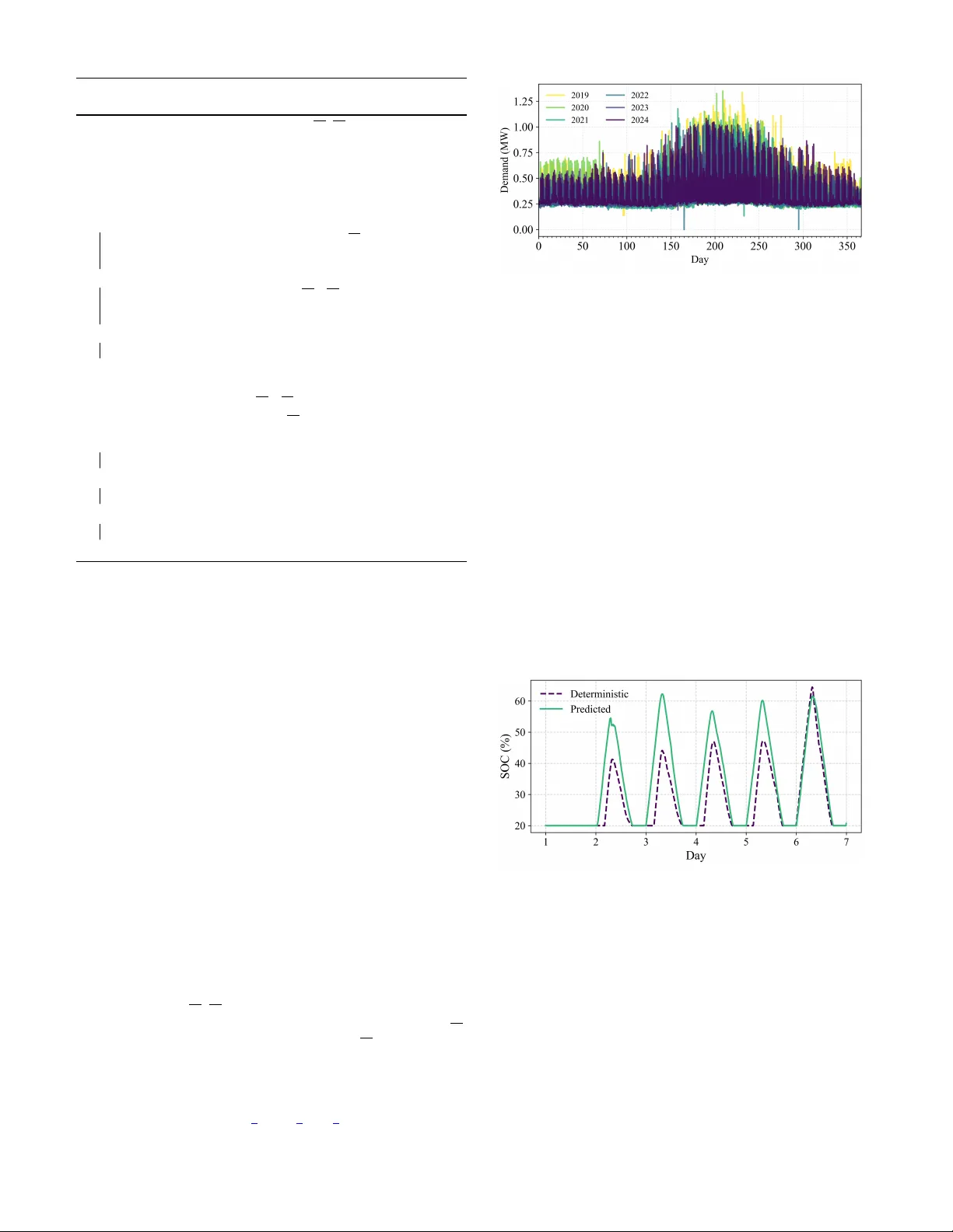
Nonparametric K ernel Re gression for Coordinated Ener gy Storage Peak Sha ving with Stacked Services Emily Logan, Ning Qi, Bolun Xu Department of Earth and En vironmental Engineering Columbia University New Y ork, NY 10027, USA { el3350, nq2176, bx2177 } @columbia.edu Abstract —Developing effective control strategies for behind- the-meter energy storage to coordinate peak sha ving and stacked services is essential f or reducing electricity costs and extending battery lifetime in commercial b uildings. This work pr oposes an end-to-end, two-stage framework for coordinating peak sha ving and energy arbitrage with a theoretical decomposition guarantee. In the first stage, a non-parametric kernel r egression model constructs state-of-charge trajectory bounds from historical data that satisfy peak-shaving requirements. The second stage utilizes the remaining capacity f or energy arbitrage via a transfer learning method. Case studies using New Y ork City commercial building demand data show that our method achieves a 1.3 times improv ement in performance over the state-of-the-art for ecast-based method, achieving cost savings and effecti ve peak management without relying on predictions. Index T erms —Peak shaving, energy storage, stacked ser vice, two-stage optimization, kernel regression I . I N T R O D U C T I O N The rapid growth of electricity demand, along with lim- ited grid infrastructure, has intensified the need for effecti ve demand-side management. Large commercial and industrial consumers are facing significant electricity costs, including both real-time electricity charges and monthly peak demand charges, with the latter being the more substantial. Behind- the-meter battery energy storage systems (BESS) ha ve thus become an attractiv e solution for peak sha ving and electricity cost reduction, while also mitigating grid stress [ 1 ], [ 2 ]. Peak shaving is challenging, as it requires decision-making under uncertainty over monthly horizons. Many existing meth- ods rely on demand and price forecasting and uncertainty mod- els such as re gression [ 3 ], neural-networks [ 4 ], and chance- constrained models [ 5 ]. Ho wev er , reliable forecasting or uncer- tainty models at a monthly resolution remain computationally intensiv e [ 6 ]–[ 8 ]. The complexity increases significantly when peak shaving is integrated with other grid services, such as energy arbitrage and frequency regulation [ 9 ], requiring careful coordination to balance the competing objectiv es. Other approaches, including dynamic programming [ 10 ] and portfolio optimization [ 11 ], ha ve also been emplo yed to op- timize stack ed storage services, but these methods primarily focus on daily peak shaving and struggle with computational burden when adapting to real-time uncertainties or extending to monthly horizons. This limits their practicality for smaller This work was partly supported by the Department of Energy under Grant No. DE-EE0011385 and by the National Science Foundation under award ECCS-2239046. businesses and non-profits, where costs may exceed the po- tential savings. W e propose an end-to-end, two-stage framew ork to coor- dinate peak shaving with stacked services such as energy arbitrage. Unlike con ventional methods that rely on forecast- ing or computationally intensiv e optimization, we propose a lightweight online optimization method to jointly predict a dynamic peak demand target and state-of-char ge (SoC) reserve trajectory for peak shaving. This enables real-time adaptiv e control under e volving demand conditions, resulting in faster and more efficient battery operation. The key contributions of this work are summarized as follo ws: 1) Decoupled Control Formulation: W e show that the stacked service control problem can be reformulated as a two-stage optimization by determining the SoC reserve required for peak shaving first, and then the remaining battery capacity is subsequently allocated to other services. 2) Kernel Regression-Based Prediction: W e dev elop a data-driv en kernel regression algorithm that jointly pre- dicts peak-shaving targets and SoC reserve requirements directly from historical demand and battery characteris- tics. 3) Joint Peak Sha ving and Arbitrage: W e integrate the kernel regression predictions with an arbitrage optimiza- tion algorithm, enabling decoupled management of peak shaving and ener gy arbitrage, reducing total electricity costs and mitigating unnecessary battery cycling. 4) V alidating P erformance thr ough Simulation: The pro- posed framew ork is ev aluated using 6 years of electricity demand data from a 35-story commercial building in New Y ork City , demonstrating improved peak shaving and cost savings compared to a state-of-the-art method. The remainder of the paper is or ganized as follows. Sec- tion II introduces the formulation, and Section III details the training and the real-time control algorithm. Section IV sho ws the simulation and Section V concludes the paper . I I . P R O B L E M F O R M U L AT I O N A N D D E C O M P O S I T I O N A. P eak Shaving and Arbitrage F ormulation W e consider a commercial building with a co-located, behind-the-meter BESS operating under a time-v arying elec- tricity tarif f. The objecti ve is to minimize the ov erall electricity cost by leveraging both energy arbitrage and peak sha ving strategies. The deterministic version of the joint peak shaving and arbitrage problem is listed as follows: F comb ( x ) = min p,d,q X T t =1 [ cd t + λ t ( D t − d t + q t )] + κp (1a) s.t. p ≥ D t − d t + q t , ∀ t = 1 , . . . , T (1b) e t +1 = e t − d t /η + η q t , ∀ t = 1 , . . . , T (1c) 0 ≤ d t , q t ≤ P , ∀ t = 1 , . . . , T (1d) E ≤ e t +1 ≤ E , ∀ t = 1 , . . . , T (1e) The decision variables include the discharge energy per timestep ( d t ), charge energy per timestep ( q t ), and peak demand within the optimization horizon ( p ). The battery’ s maximum ener gy capacity and energy capacity per timestep are denoted by E and P , respecti vely . E denotes the minimum SoC bound and η denotes the efficiency for charging and discharging. The objectiv e function in ( 1a ) minimizes total cost by balancing peak demand charges ( κ ), real-time ener gy price ( λ ), and battery degradation cost ( c ). The model includes constraints for battery behavior and peak shaving. ( 1b ) defines p as the maximum net demand. SoC dynamics are updated by ( 1c ), and ( 1d ) and ( 1e ) enforce power and energy limits. B. Decomposition of Stack ed Services The deterministic formulation of the problem in ( 1 ) is impractical to solv e in practice, as both demand and elec- tricity prices are uncertain, while the peak demand charge is typically settled on a monthly basis. Solving the problem ov er such a long uncertainty horizon is therefore computationally intractable. T o address this challenge, based on the fact that the peak penalty κ is much lar ger than the energy cost coef ficients c and λ t in practice, ( 1 ) can be effecti vely decomposed into two sequential subproblems. This decomposition first prioritizes minimizing peak demand and then performs energy arbitrage ov er the resulting feasible set. Peak Shaving. In the first stage, we minimize the peak demand and determine the associated trajectory of the SoC reserve necessary for peak sha ving. In comparison to the objectiv e in ( 1 ), we introduce a small tie-breaking term δ P T t =1 e t +1 in the objective. This term keeps SoC levels lo w but does not affect the peak value when δ is suf ficiently small. Solving ( 2 ) thus yields an optimal peak demand p ∗ and SoC profile e ∗ . F PS ( x ; δ ) = min p,d,q ,e p + δ X T t =1 e t +1 s.t. Constraints ( 1b )–( 1e ) (2) Arbitrage. Gi ven the Stage 1 solution ( p ∗ , e ∗ ), Stage 2 max- imizes the revenue from energy arbitrage while ensuring that arbitrage decisions respect both the peak shaving constraint p ≤ p ∗ and the SoC trajectory established in Stage 1. F arb ( x ) = min d,q ,e X T t =1 [ cd t − λ t ( d t − q t )] (3a) s.t. p ∗ ≥ D t − d t + q t , ∀ t = 1 , . . . , T (3b) e t +1 ≥ e ∗ t +1 , ∀ t = 1 , . . . , T (3c) ( 1c ) − ( 1e ) . W e no w present the following proposition proving that the decomposition is equiv alent to the original problem: Proposition 1. Given that δ is sufficiently small and κ ≫ λ t , c , solving the two-stag e optimization in ( 2 ) and ( 3 ) is equivalent to solving the combined peak shaving and arbitrage pr oblem in ( 1 ) . Pr oof. W e first restate the combined problem for con venience: F comb ( x ) = X T t =1 λ t D t + F arb ( x ) + κF PS ( x ) . Let x = ( p, { d t , q t , e t +1 } T t =1 ) denote the decision variables, and let S be the feasible region defined by ( 1b )–( 1e ), where g ( x ) ≤ 0 collects all inequality constraints and h ( x ) = 0 the equality constraint. The Lagrangian of the combined problem is L comb ( x, µ, ν ) = F arb ( x ) + κF PS ( x ) + µ T g ( x ) + ν T h ( x ) , (4) with µ ≥ 0 and ν denoting the dual variables. The KKT stationarity condition is ∇ x F arb ( x ) + κ ∇ x F PS ( x ) + ∇ g ( x ) T µ + ∇ h ( x ) T ν = 0 , (5) accompanied by primal and dual feasibility and complemen- tary slackness. T o analyze the limit κ ≫ λ t , c , define rescaled dual variables ˜ µ = µ/κ and ˜ ν = ν /κ . Substituting into ( 5 ) and dividing by κ yields ∇ x F arb ( x ) /κ + ∇ x F PS ( x ) + ∇ g ( x ) T ˜ µ + ∇ h ( x ) T ˜ ν = 0 . (6) T aking the limit as κ → ∞ remov es the first term, giving ∇ x F PS ( x ) + ∇ g ( x ) T ˜ µ + ∇ h ( x ) T ˜ ν = 0 , (7) which are precisely the KKT conditions of the peak shaving problem. Thus, for κ ≫ λ t , c and δ → 0 + , the solution to ( 1 ) coincides with the peak shaving optimum: p ∗ comb = p ∗ and e ∗ comb = e ∗ . Since the combined solution minimizes F PS ( x ) under these conditions, it lies in the optimal peak shaving set S ∗ = { x ∈ S | F PS ( x ) = F ∗ PS } . Restricting the combined problem to S ∗ , we hav e: min x ∈ S ∗ [ F arb ( x ) + κF PS ( x )] . As F PS ( x ) = F ∗ PS for all x ∈ S ∗ , the constant term κF ∗ PS can be dropped, leaving min x ∈ S ∗ F arb ( x ) , identical to the arbitrage formulation ( 3 ) ov er the feasible set characterized by p ≤ p ∗ and e t +1 ≥ e ∗ t +1 for all t . Therefore, when κ is sufficiently large, solving the com- bined problem ( 1 ) is equiv alent to the two-stage procedure of first solving the peak shaving problem ( 2 ) to obtain ( p ∗ , e ∗ ) , and then optimizing arbitrage ov er S ∗ . In this work, our primary contrib ution is the development and e valuation of a peak shaving strate gy , including its inte gra- tion with other stacked services. Energy arbitrage is handled using an established non-anticipatory policy from [ 12 ]. I I I . L E A R N I N G A N D C O N T RO L M E T H O D W e now present our main methods for deriving a non- anticipatory algorithm to solve the joint peak shaving and arbitrage problem using the decomposition approach. Our general approach is as follows: 1) we use historical demand data to generate the SoC reserv e and daily net demand tar gets deriv ed from monthly peak shaving results; 2) we use a kernel regression algorithm with a look-back demand window to jointly predict the SoC reserve target and the peak shaving target; 3) we input the predicted SoC reserve target into a real-time peak shaving and arbitrage controller . A. K ernel Regr ession for SoC Reserve Pr ediction The kernel re gression model predicts the minimum SoC re- serve required for peak sha ving at each timestep by comparing the current demand pattern to historically observed demand trajectories. W e first use historical demand data and solve ( 2 ) to generate the hindsight-optimal SoC reserve target e hist s and the net demand for each timestep. From the latter, we extract the maximum v alue within each day , which we define as the hindsight-optimal peak shaving target p hist s . Note that we use s to represent the time index in the training data and t in the real-time control to reduce confusion of the time index. T raining data generation. Let the full historical demand record be D hist = { D hist 1 , . . . , D hist N } , where N is the total number of historical timesteps. Let T be the length of the sliding demand windows. Demand look-back vectors are con- structed as D hist s = [ D hist s − T +1 , . . . , D hist s ] , where each windo w endpoint s is associated with a corresponding next minimum SoC reserv e e hist s +1 and peak shaving tar get p hist s +1 obtained from the prior training results. Hence each training data entry can be represented as { e hist s +1 , p hist s +1 | X hist s = [ D hist s , t sin ,s , t cos ,s ] } (8) where t sin ,t and t cos ,t are sine and cosine vectors with a daily period to capture the time-of-the-day feature. Prediction Featur e. In prediction, we assemble the input feature similarly to X hist s . Let the observed demand sequence up to the current timestep t be D = { D 1 , . . . , D t } , and at each timestep t ≥ T , the most recent sequence of T demand values is represented as D t = [ D t − T +1 , . . . , D t ] . The prediction feature vector is thus assembled as X t = [ D t , t sin ,t , t cos ,t ] , (9) α -Confidence Ker nel Regression. F or each current feature vector X t , the set of K most similar historical v ectors, denoted KNN( t ) , is identified using Euclidean distance. The similarity between X t and each neighbor X hist s is quantified using a Gaussian kernel, and the resulting weights are normalized across the K nearest n e ighbors so that they sum to one: w t,s = exp  −∥ X t − X hist s ∥ 2 2 / (2 T σ 2 )  P j ∈ KNN( t ) exp  −∥ X t − X hist j ∥ 2 2 / (2 T σ 2 )  . (10) where s ∈ KNN( t ) and σ is the kernel bandwidth parameter that controls ho w rapidly the influence of historical windows decays with dissimilarity to the current feature profile. The resulting weights w t,s are used to compute the pre- dicted required SoC reserve at each timestep. W e introduce a confidence-lev el parameter α ∈ (0 , 1) to provide a tunable conservati veness ensuring the predicted SoC reserv e is greater than α ratio of the training data. The predicted SoC for the next time step t + 1 is therefore ˆ e α t +1 = e hist k + α − W t,k W t,k − W t,k − 1 ( e hist k − e hist k − 1 ) (11a) where W t,k − 1 ≤ α ≤ W t,k (11b) W t,k = P k i =1 w t,k (11c) k is the ascending rank of e hist s +1 , s ∈ KNN( t ) (11d) The historical SoC reserve values of the K nearest neigh- bors are sorted in ascending order , and their corresponding weights are summed. The SoC value at which the cumulativ e weight first reaches α is selected as the predicted SoC reserve, allowing the estimate to be adjusted to be more conserv ativ e or aggressiv e depending on operational preferences. Unlike the SoC reserve, the peak shaving target p pred t +1 is computed as a simple weighted av erage: p pred t +1 = X s ∈ K N N ( t ) w t,s p hist s , s ∈ K N N ( t ) . (12) No confidence-level adjustment is applied here because the real-time controller described in Section III-B dynamically adapts peak-sha ving targets based on the observed net demand, ensuring conservati veness is enforced through the adaptive control rather than through the kernel regression itself. B. Real-T ime Contr ol Based on the predicted SoC reserve estimates and daily net demand targets, a real-time controller determines the battery charge schedule, discharge schedule, and SoC trajectory to achiev e peak shaving while ensuring feasible operation. This SoC trajectory establishes the energy that must be reserved for peak shaving at each time step. The remaining battery capacity can then be allocated to additional services, such as arbitrage. The control logic operates as described by Algorithm 1 . C. P arameter Sear ch The kernel re gression model relies on three key hyper- parameters—the kernel bandwidth σ , the look-back window T , and the number of nearest neighbors K , which directly influence the performance of the combined peak shaving and arbitrage strategy . Performance is e valuated using two metrics: (1) total cost savings , defined as the reduction in electricity cost relati ve to a no-storage baseline, and (2) annual battery cycles , calculated as the total discharge energy divided by the nominal battery capacity E , indicating utilization and wear . T o systematically identify effecti ve h yperparameters, we implement an automated, tiered search that adaptiv ely tunes each in sequence. The look-back window T is optimized first through a coarse-to-fine search to find the most informati ve time horizon. Next, the kernel bandwidth σ is tuned using a logarithmic-scale exploration follo wed by linear refinement to Algorithm 1: Real-T ime Peak Sha ving and Stacked Services Control Input: D t , e t , ˆ e α t +1 , p t − 1 , p pred t +1 , ( P , E , η ) , q t,arb , d t,arb [ 12 ]. Output: q t , d t , e t +1 , p t +1 , D net t . Stage 1: Peak Shaving ∆ e t = ˆ e α t +1 − e t ; p t = max { p t − 1 , p pred t +1 } if D t > p t then d t, PS = min(max( − ∆ e t η , D t − p t ) , P , e t η ) ; q t, PS = 0 else if e t < ˆ e α t +1 and D t < p t then q t, PS = min(∆ e t /η , p t − D t , P , ( E − e t ) /η ) ; d t, PS = 0 else q t, PS = d t, PS = 0 e t +1 , PS = e t − d t, PS /η + q t, PS η ; p t +1 = max { p t , D net t } Stage 2: Arbitrage q t, max = min( p t +1 − D t , P , ( E − e t ) /η ) ; d t, max = min(( e t − e t +1 , PS ) η , P ) if q t, PS > 0 then q t = min( q t, arb + q t, PS , q t, max ) ; d t = 0 else if d t, PS > 0 then d t = min( d t, arb + d t, PS , d t, max ) ; q t = 0 else q t = min( q t, arb , q t, max ) ; d t = min( d t, arb , d t, max ) e t +1 = e t − d t /η + q t η ; D net t = D t − d t + q t strike a balance between accuracy and smoothness. Finally , the number of nearest neighbors K is adjusted through broad and refined searches to maximize performance. I V . S I M U L A T I O N A N D R E S U L T S W e conduct a real-world case study of a 35-story , 800 , 000 ft 2 , Class A commercial building in New Y ork City . The demand data for this building, provided by Nantum AI 1 , is sho wn in Fig. 1 . Peak demand charges follow Con Edison’ s standard rate, which applies a charge of $42.80/kW to the monthly peak demand from June 1 to September 30 and $33.50/kW during other months, plus a flat monthly customer charge of $71. The monthly peak demand is defined as the av erage of the two highest consecuti ve 15-minute interv als of demand 2 . Arbitrage is performed using real-time electricity prices from the New Y ork Independent System Operator 3 . T o account for seasonal patterns in demand and pricing, the kernel regression model considers only historical data from the same season (either June–September or the other months) when predicting SoC reserve and net demand targets. Historical building data from 2019–2023 is used for model training, and the data from 2024 is reserved for testing. The battery duration ( E /P ) is 2.2 hours, with an initial state of charge (SoC) of 50% ( e 0 ), a minimum SoC ( E ) of 20% of E , and an efficienc y ( η ) of 90%. Parameters are selected by the automatic algorithm described in Section III-C . All simulations are conducted at a 5-minute resolution on a 10-core Apple 1 https://github .com/emlog9/peak shaving kernel regression 2 https://www .coned.com/en/accounts- billing/your- bill/time- of- use 3 https://www .nyiso.com/energy- mark et- operational- data Fig. 1. Building electricity demand from 2019–2024. Line colors indicate years. Y early standard de viations are: 2019: 0.21 MW , 2020: 0.16 MW , 2021: 0.16 MW , 2022: 0.16 MW , 2023: 0.18 MW , and 2024: 0.19 MW . M4 processor , and all optimization problems are solved using Gurobi 12.0.2. Model performance is ev aluated based on total cost savings compared to the no-storage scenario and battery cycling. The results for peak sha ving and arbitrage are compared against two benchmarks: (i) the deterministic case outlined in ( 1 ), limited to an average of one c ycle per day , and (ii) a demand-forecasting controller based on a recursiv e XGBoost model with a mean absolute error (MAE) of 0.03 MW . This model utilizes calendar features, temperature, and lagged demand to generate day-ahead demand forecasts, which are then input into the peak shaving optimization from ( 2 ). From there, the real-time controller determines the char ge and discharge schedule. As with the kernel regression framew ork, these results are subsequently combined with an arbitrage schedule from [ 12 ] in a two-stage approach. Simulations are performed for battery power ratings ranging from 0.1 MW to 1.0 MW . Fig. 2. Comparison of the kernel-regression predicted and deterministic minimum SoC reserve trajectories for a 1 MW battery . Fig. 2 compares the predicted SoC reserve trajectory to the deterministic SoC trajectory for a representati ve week. The predicted SoC generally tracks the timing and magnitude of the actual SoC peaks, though it tends to slightly ov erestimate the reserve. This behavior aligns with the design of the confidence lev el parameter ( α ), which accounts for uncertainty by allowing for more conservati ve SoC predictions. Fig. 3 shows the peak demand across the three controller types in comparison to the peak demand with no battery storage. Overall, the kernel regression controller ef fectively shav es the peak demand, outperforming the demand forecast- ing model in most months. Fig. 3. Peak demand (MW) by month for perfect foresight, kernel regression- based, and demand forecasting control algorithms for a 0.6 MW battery . T o e valuate the economic impact of the proposed control strategy , we analyze annual cost savings relativ e to a scenario with no storage, where the total electricity cost is $512.5k, as a function of battery power capacity (MW). This metric captures the economic benefit of combined peak shaving and energy arbitrage given real-time electricity prices and demand patterns. Fig. 4 compares the results for the kernel re gres- sion–based controller with the deterministic and demand- forecasting baseline cases. Fig. 4. T otal annual cost savings (%) vs. battery size for perfect foresight, kernel regression-based, and demand forecasting control algorithms. Larger batteries achie ve higher savings, although the in- creasing trend saturates. Across the battery sizes e valuated in this study , the kernel regression model captures between 38.1% and 58.5% of the deterministic cost savings, outperforming the demand forecasting controller for each battery size, which achiev es only 33.0% to 39.8% of the deterministic cost sav- ings. It is worth noting that the deterministic perfect foresight assumes one month of perfect demand and price forecast (based on a monthly utility bill settlement). Consequently , the performance of the perfect forecast is significantly better . Battery c ycling is an important metric for understanding bat- tery utilization and wear . The deterministic controller operates near its cycle limit of one cycle per day on av erage, ranging from 346 to 366 cycles annually across the range of battery power capacities (0.1 MW to 1 MW). This beha vior indicates that with perfect foresight, maximizing cost savings and fully exploiting peak shaving and arbitrage opportunities requires aggressiv e daily cycling. In contrast, the k ernel regression controller e xhibits more v ariable c ycling, ranging from approx- imately 76 to 126 c ycles per year across battery sizes. This variation arises because the controller relies on predicted SoC trajectories rather than perfect knowledge of future demand and prices. Underestimation or o verestimation of the SoC can cause missed opportunities to charge or discharge at optimal times. The demand forecasting model c ycles ev en less, ranging from 57 to 95 annual cycles. V . C O N C L U S I O N This work presents an end-to-end frame work for behind-the- meter peak shaving and stacked energy services in commercial buildings. The method employs a two-stage decomposition, where a nonparametric kernel regression model generates a state-of-charge reserve trajectory for real-time peak shaving control without requiring e xplicit demand forecasts. The re- maining battery capacity is then allocated to energy arbitrage via a non-anticipatory control strategy . A real-world case study demonstrates that the proposed approach outperforms a standard demand forecasting baseline, capturing 38.1%–58.5% of the cost savings achieved by a perfect-foresight benchmark. The results highlight the method’ s practicality and economic effecti veness for real-time battery management. For future work, we aim to enhance the kernel regression model and integrate additional services such as frequency regulation. R E F E R E N C E S [1] J. Li, G. Mu, J. Zhang, C. Li, G. Y an, H. Zhang, and G. Chen, “Dynamic economic e valuation of hundred mega watt-scale electrochemical energy storage for auxiliary peak sha ving, ” Pr otection and Contr ol of Modern P ower Systems , v ol. 8, no. 3, pp. 1–18, 2023. [2] B. T . Mirletz and N. D. Laws, “Impacts of dispatch strategies and fore- cast errors on the economics of behind-the-meter pv-battery systems, ” National Renewable Energy Laboratory (NREL), Golden, CO, USA, T ech. Rep. NREL/CP-7A40-86194, July 2023. [3] R. T . de Salis, A. Clarke, Z. W ang, J. Moyne, and D. Tilb ury , “Energy storage control for peak shaving in a single building, ” IEEE PES Gener al Meeting , pp. 1–5, 2014. [4] X. Zhang, T . K. Chau, Y . H. Chow , T . Fernando, and H. H.-C. Iu, “ A novel sequence to sequence data modelling based cnn-lstm algorithm for three years ahead monthly peak load forecasting, ” IEEE T ransactions on P ower Systems , v ol. 39, no. 1, pp. 1932–1947, 2023. [5] N. Qi, P . Pinson, M. R. Almassalkhi, L. Cheng, and Y . Zhuang, “Chance- constrained generic energy storage operations under decision-dependent uncertainty , ” IEEE T ransactions on Sustainable Ener gy , vol. 14, no. 4, pp. 2234–2248, 2023. [6] M. Kaut, “Handling of long-term storage in multi-horizon stochastic programs, ” Computational Management Science , vol. 21, no. 1, p. 27, 2024. [7] C. Cortes-Aguirre, Y .-A. Chen, A. Ghosh, J. Kleissl, and A. Khurram, “Economic mpc with an online reference trajectory for battery schedul- ing considering demand charge management, ” IEEE T ransactions on Smart Grid , 2025. [8] Y . Mo, Q. Lin, M. Chen, and S.-Z. J. Qin, “Optimal online algorithms for peak-demand reduction maximization with energy storage, ” in Pr o- ceedings of the twelfth A CM international confer ence on future ener gy systems , 2021, pp. 73–83. [9] Y . Shi, B. Xu, D. W ang, and B. Zhang, “Using battery storage for peak sha ving and frequenc y regulation: Joint optimization for superlinear gains, ” IEEE transactions on power systems , vol. 33, no. 3, pp. 2882– 2894, 2017. [10] J. Engels, B. Claessens, and G. Deconinck, “Optimal combination of frequency control and peak shaving with battery storage systems, ” IEEE T ransactions on Smart Grid , v ol. 11, no. 4, pp. 3270–3279, 2020. [11] N. Qi, L. Cheng, H. Li, Y . Zhao, and H. T ian, “Portfolio optimization of generic energy storage-based virtual power plant under decision- dependent uncertainties, ” J ournal of ener gy storag e , vol. 63, p. 107000, 2023. [12] Y . Baker , N. Zheng, and B. Xu, “Transferable ener gy storage bidder, ” IEEE Tr ansactions on P ower Systems , vol. 39, no. 2, pp. 4117–4126, 2023.