Learning Distributed Equilibria in Linear-Quadratic Stochastic Differential Games: An $α$-Potential Approach

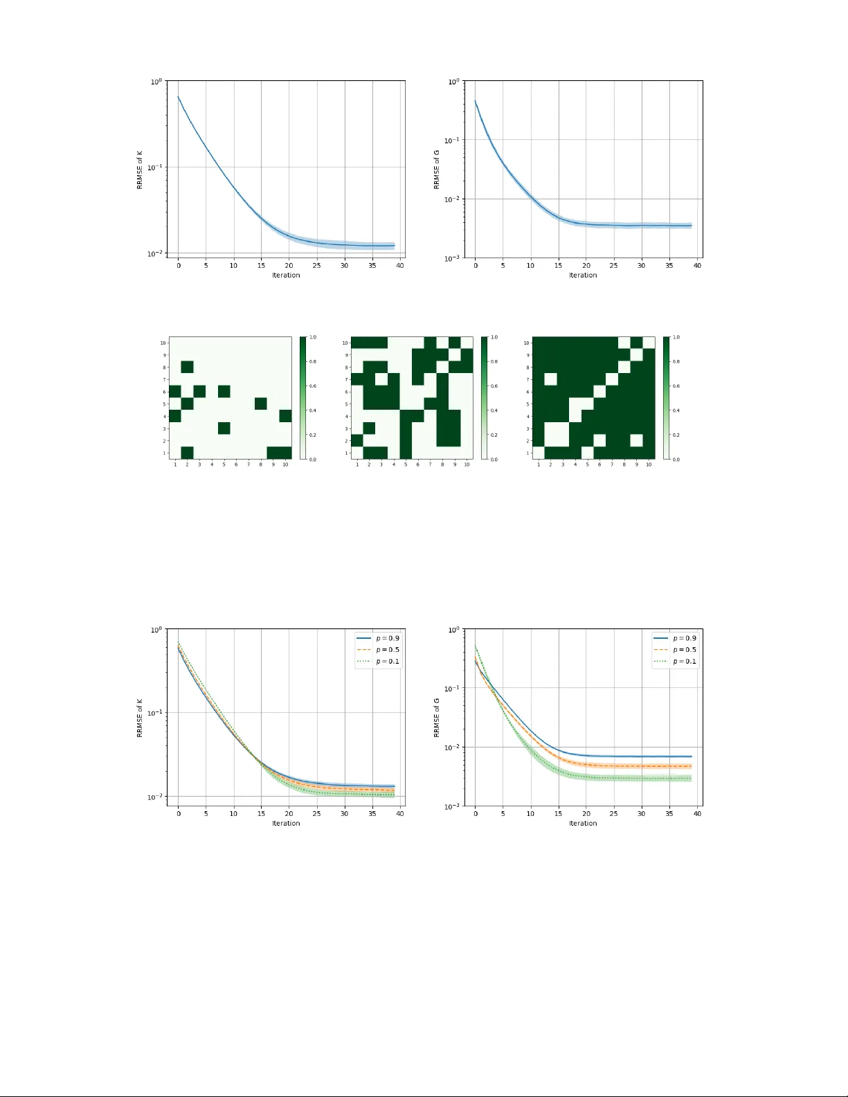
Learning Distributed Equilibria in Linear-Quadratic Sto c hastic Diﬀeren tial Games: An α -P oten tial Approac h Philipp Plank ∗ Y ufei Zhang ∗ Abstract W e analyze indep enden t p olicy-gradien t (PG) learning in N -pla yer linear-quadratic (LQ) sto c hastic diﬀeren tial games. Each pla yer emplo ys a distributed policy that dep ends only on its o wn state and up dates the policy indep enden tly using the gradient of its o wn ob jectiv e. W e establish global linear conv ergence of these metho ds to an equilibrium by sho wing that the LQ game admits an α -p oten tial structure, with α determined by the degree of pairwise interaction asymmetry . F or pairwise-symmetric interactions, we construct an aﬃne distributed equilibrium b y minimizing the p oten tial function and show that indep enden t PG methods con verge globally to this equilibrium, with complexity scaling linearly in the p opulation size and logarithmically in the desired accuracy . F or as ymmetric in teractions, we pro ve that independent pro jected PG algorithms con verge linearly to an appro ximate equilibrium, with sub optimalit y proportional to the degree of asymmetry . Numerical exp erimen ts conﬁrm the theoretical results across b oth symmetric and asymmetric interaction netw orks. Keyw ords. Linear-quadratic sto c hastic diﬀeren tial game, distributed equilibria, α -potential game, indep enden t learning, p olicy gradient, global con vergence AMS sub ject classiﬁcations. 91A06, 91A14, 91A15, 91A43, 49N10, 68Q25 1 In tro duction Can m ulti-agent reinforcement learning (MARL) algorithms reliably and eﬃciently learn Nash equilibria (NEs) in N -play er non-co op erativ e sto c hastic diﬀerential games? These games mo del strategic in teractions among m ultiple pla yers, each con trolling a stochastic diﬀeren tial system and optimizing an ob jective inﬂuenced by the actions of all pla yers. They arise naturally in div erse ﬁelds, including autonomous driving [ 8 ], neural science [ 4 ], ecology [ 33 ], and optimal trading [ 30 ]. A central goal is the computation of NEs, p olicy proﬁles from which no play er can impro ve its pay oﬀ through unilateral deviation. In man y settings, such equilibria are analytically in tractable, motiv ating growing in terest in learning-based approaches that approximate NEs from data collected through rep eated interactions with the en vironment. Despite this promise, MARL algorithms with theoretical p erformance guarantees for stochastic diﬀeren tial games are still limited, due to three fundamental challenges inheren t in multi-agen t in teractions. First, scalabilit y b ecomes a critical issue ev en with a mo derate n umber of play ers, as the complexity of the joint strategy space grows exp onen tially with the p opulation size [ 18 , 12 ]. Second, eac h individual play er faces a non-stationary environmen t, as other pla yers are sim ultaneously learning and adapting their p olicies. The analysis of MARL algorithms thus ∗ Departmen t of Mathematics, Imp erial College London, London, UK ( p.plank24@imperial.ac.uk, yufei.zhang@imperial.ac.uk ) 1 necessitates no vel game-theoretic techniques b ey ond the single-agent setting. Third, diﬀerential games t ypically in volv e con tin uous time and con tinuous state or action spaces, requiring the use of function appro ximation for p olicies. The choice of policy parameterization can signiﬁcan tly aﬀect b oth the eﬃciency and conv ergence of MARL algorithms. As an initial step to tackle the aforementioned challenges, this w ork inv estigates the conv er- gence of p olicy gradient (PG) algorithms for N -play er linear-quadratic (LQ) games. LQ games pla y a fundamental role in dynamic game theory , and serv e as b enc hmark problems for examining the p erformance of MARL algorithms [ 28 , 17 , 20 , 31 ]. Despite their relative tractability , existing w ork s ho ws that gradient-based learning algorithms ma y fail to conv erge to NEs [ 28 ], or conv erge only under restrictive con traction conditions that do not scale well with the p opulation size or the time horizon [ 17 , 31 ]. Indep enden t learning with distributed p olicies. T o ensure scalability , we adopt distrib- ute d (also known as decentralized) p olicies and focus on indep endent PG metho ds. A distributed p olicy means that each play er bases its feedback control solely on its own state, without consid- ering the states of other play ers. This approach reduces the need for inter-pla y er communication and simpliﬁes the p olicy parameterization. Indep enden t PG algorithms further assume that each pla yer up dates its p olicy indep enden tly and concurrently by following the gradien t of its own ob- jectiv e. Combining indep enden t learning with distributed p olicies ensures that the computational complexit y of the algorithm scales line arly with the n umber of play ers. Although distributed p olicies are widely used in MARL [ 18 ], the existence and characteriza- tion of NEs in the resulting N -play er games ha ve not b een rigorously studied, and no theoretical guaran tees currently exist for the corresp onding PG metho ds. An exception arises in mean ﬁeld games, where pla yers are assumed to interact symmetric al ly and we akly through empirical meas- ures. Under this assumption, appro ximate distributed NEs for N -pla yer games can be constructed via a limiting contin uum mo del as N → ∞ (see e.g., [ 5 , 24 , 31 ]). How ev er, in many realistic set- tings, play ers are not exc hangeable and instead interact only with subsets of play ers sp eciﬁed by an underlying net work. Moreo v er, the inﬂuence of each play er on others ma y not v anish as the p opulation size gro ws [ 8 ]. This motiv ates the study of general interaction structures under which distributed NEs can b e characterized and learned. Our contributions. This work pro vides non-asymptotic p erformance guarantees for indep end- en t PG algorithms in approximating distributed NEs in a class of ﬁnite-horizon N -pla yer LQ games, inspired by ﬂocking mo dels [ 23 , 14 ] and opinion formation mo dels [ 2 ]. In this game, each pla yer i c ho oses a distributed p olicy to linearly con trol the drift of its state dynamics and minim- izes a cost that is quadratic in its o wn con trol and in the states of all pla yers, with the inﬂuence of the pro duct of play ers j and k ’s states w eighted by Q i k,j (see ( 2.1 )-( 2.2 ) for precise deﬁnitions). W e analyze this LQ game and the asso ciated learning algorithms by extending the α -p otential game framework developed in [ 14 , 13 , 15 ] to closed-lo op games with distributed p olicies. In an α -p oten tial game, when a pla yer c hanges its strategy , the resulting change in its ob jective aligns with the c hange in an α -p otential function up to an error α . • W e pro ve that the LQ game is an α -potential game, with an α -potential function form ulated as a distributed LQ con trol problem. The parameter α is explicitly characterized b y the pro duct of the constant C Q = max 1 ≤ i ≤ N P N j =1 | Q i i,j − Q j j,i | and b ounds on the ﬁrst and second momen ts of the state dynamics induced by admissible p olicies (Prop osition 2.3 ). • When C Q = 0, i.e., the interaction is p airwise symmetric , we prov e that the game admits an aﬃne equilibrium, giv en by the minimizer of the p oten tial function (Theorem 3.2 ). In this 2 equilibrium, eac h play er’s action dep ends linearly on the deviation of its own state from its exp ected v alue, adjusted by a time-dep enden t intercept term. W e further prov e that an indep enden t PG algorithm, in which eac h pla yer updates the slop e and in tercept parameters of its p olicy independently via gradient descen t, con verges globally to the NE p olicy at a linear rate. This implies that the algorithm’s complexit y to achiev e an error of ε scales line arly with the p opulation size N and with log(1 /ε ). The pro of leverages the p oten tial structure by interpreting the learning algorithm as a PG metho d applied to the p otential function and b y exploiting the geometry of the p oten tial function with resp ect to the p olicy proﬁles (Prop ositions 3.5 and 3.6 ). • F or general interactions with C Q > 0, we characterize aﬃne equilibria through a forward- bac kward ordinary diﬀerential equation (ODE) system (Theorem 4.1 ) and pro vide suﬃcient conditions for the existence of an NE (Prop osition 4.2 ). W e further prov e that an indep end- en t pro jected PG algorithm conv erges linearly to an approximate NE, with the appro xima- tion error scaling prop ortionally with the constant C Q (Theorem 4.6 ). The pro of relies on in terpreting the learning algorithm as a biased PG metho d for the α -p oten tial function and on quan tifying the bias through a stability analysis of the asso ciated ODEs. T o the b est of our knowledge, this work pro vides the ﬁrst global conv ergence result for inde- p enden t PG metho ds in contin uous-time LQ games with general non-exchangeable interactions. Challenges b ey ond existing works. The characterization of distributed NEs requires nov el tec hniques b ey ond standard LQ games with full-information p olicies. When C Q = 0, we construct an NE by minimizing the potential function. This reduces to a distributed control problem, whic h w e solve using a dynamic programming approach as in [ 21 ]. Sp eciﬁcally , we lift the problem to a McKean-Vlasov control problem ov er the space of pro duct measures and solve the resulting inﬁnite-dimensional Hamilton-Jacobi-Bellman (HJB) equations. In the general case with C Q > 0, w e characterize the NE by a coupled system, consisting of N bac kward HJB equations, which determine eac h play er’s optimal p olicy given other play ers’ state distributions, and N forw ard F okker-Planc k equations, whic h describ e the state ev olution under these p olicies. Analyzing indep endent PG metho ds for LQ games also presen ts challenges b ey ond those in prior studies of discrete-time Mark ov ( α -)p oten tial games with ﬁnite state and action spaces (see e.g., [ 9 , 10 , 25 , 35 , 22 , 27 , 13 ]). First, existing analyses typically quan tify algorithm con vergence in terms of the cardinality of the state and action spaces. This approac h is inapplicable to con tinuous-time LQ games, whic h in volv e contin uous state and action spaces and p olicies that v ary contin uously with time. In fact, even for discrete-time LQ games with distributed p olicies, existing results only establish asymptotic conv ergence of PG metho ds to saddle p oin ts, rather than to NEs, and do not provide conv ergence rates [ 20 ]. W e substantially strengthen these results b y proving linear conv ergence to NEs. Achieving this requires a more reﬁned landscap e analysis that characterizes the geometry of the cost functions with resp ect to the p olicy parameters, which is enabled b y an appropriate choice of p olicy parameterization (Remark 3.1 ). Second, analyzing algorithm conv ergence for α > 0 is tec hnically in volv ed. In this setting, the gradien t of eac h play er’s ob jectiv e constitutes a biased gradient of the α -p oten tial function, with the bias scaling with α . Moreo ver, as sho wn in Prop osition 2.3 , when C Q > 0, the magnitude of α dep ends critically on the regularity of the p olicies. It is therefore essential to ensure that this p olicy regularity is preserved uniformly throughout the learning pro cess and to control ho w the bias propagates across iterations. 3 Notation. F or a Euclidean space E , we denote by ⟨· , ·⟩ the standard scalar pro duct, and b y |·| the induced norm. F or a matrix A ∈ R d × k , we denote b y A ⊤ the transp ose of A , and by λ max ( A ) and λ min ( A ) the largest and smallest eigen v alue of A , resp ectiv ely . F or eac h n ∈ N , w e denote b y S n ≥ 0 the space of n × n symmetric p ositiv e semideﬁnite matrices. W e introduce the following function spaces: C ([0 , T ] , E ) is the space of con tinuous functions f : [0 , T ] → E ; L 1 ([0 , T ] , E ) (resp. L ∞ ([0 , T ] , E )) is the space of Borel measurable functions f : [0 , T ] → E such that ∥ f ∥ L 1 : = R T 0 | f ( t ) | dt < ∞ (resp. ∥ f ∥ L ∞ : = ess sup t ∈ [0 ,T ] | f ( t ) | < ∞ ); and L 2 ([0 , T ] , E ) is the space of Borel measurable functions f : [0 , T ] → E with ﬁnite L 2 -norm ∥ · ∥ L 2 induced b y the canonical inner pro duct ⟨· , ·⟩ L 2 . F or any square-integrable random v ariable X deﬁned on a probabilit y space (Ω , F , P ), we denote b y E [ X ] its expectation and by V [ X ] its v ariance. 2 Distributed equilibria for sto c hastic LQ games This section introduces a class of LQ sto chastic diﬀerential games with distributed p olicies. In these games, each play er controls the drift of a linear sto c hastic diﬀerential equation through a p olicy that dep ends solely on its own state, and aims to minimize a quadratic cost functional that dep ends on b oth its individual control and the joint state of all play ers. 2.1 Mathematical setup Let T > 0 b e a given terminal time, N ∈ N b e the num b er of play ers, and I : = { 1 , 2 , . . . , N } b e the index set of play ers. Let (Ω , F , P ) b e a probability space which supp orts an N -dimensional Bro wnian motion B = ( B 1 , . . . , B N ) ⊤ , and mutually indep enden t random v ariables ( ξ i ) i ∈ I . The random v ariables ξ i and B i represen t the initial condition and the idiosyncratic noise of the state pro cess for play er i . W e assume that ξ i , i ∈ I , has a p ositiv e v ariance V [ ξ i ] > 0. W e consider a sto c hastic diﬀerential game with distributed p olicies deﬁned as follows. F or eac h i ∈ I , play er i chooses a p olicy from the set ˜ V i ⊂ V i , where V i is the set of all measurable functions u i : [0 , T ] × R → R suc h that the asso ciated state dynamics dX i t = u i ( t, X i t ) dt + σ i t dB i t , t ∈ [0 , T ]; X i 0 = ξ i (2.1) admits a unique strong solution X u i ,i satisfying E [sup t ∈ [0 ,T ] | X u i ,i t | 2 ] + E [ R T 0 | u i ( t, X u i ,i t ) | 2 dt ] < ∞ . The precise deﬁnition of ˜ V i will b e provided later in the appropriate context. W e say an y p olicy in V i is distributed since it dep ends only on play er i ’s own state. Let ˜ V : = Q i ∈ I ˜ V i b e the set of admissible p olicy proﬁles of all play ers. Play er i aims to minimize the follo wing cost functional J i : ˜ V → R : J i ( u ) : = E  Z T 0  | u i ( t, X i t ) | 2 + X ⊤ t Q i X t  dt + γ i | X i T − d i | 2  , (2.2) where X : = ( X 1 , . . . , X N ) ⊤ dep ends on u through the dynamics ( 2.1 ). T o simplify the notation, this explicit dep endence is omitted whenever there is no risk of confusion. W e assume σ i ∈ C ([0 , T ] , R ), Q i ∈ S N ≥ 0 , γ i ≥ 0 and d i ∈ R . W e denote by G = ( I , ( J i ) i ∈ I , ˜ V ) the game deﬁned b y ( 2.1 )-( 2.2 ), emphasizing its dep endence on the admissible p olicy proﬁles ˜ V . F or each i ∈ I , w e denote by ˜ V − i = Q j ∈ I \{ i } ˜ V j the set of p olicy proﬁles of all play ers except play er i . When ˜ V i = V i , w e write V = ˜ V and V − i = ˜ V − i . R emark 2.1 . F or ease of exp osition, we ha v e assumed that each play er has one-dimensional state and control processes in ( 2.1 ), and that the terminal cost of ( 2.2 ) dep ends only on play er i ’s state. 4 All results can b e extended to multi-dimensional state dynamics of the form dX i t = ( A i t X i t + D i t u i ( t, X i t )) dt + σ i t dB i t , and to terminal costs that dep end on all pla yers’ joint states. No w we introduce the deﬁnition of an ε -Nash equilibrium ( ε -NE) for the game. Deﬁnition 2.1. A p olicy proﬁle u ∗ = ( u ∗ ,i ) i ∈ I ∈ ˜ V is called a (distributed) ε -Nash equilibrium in the p olicy class ˜ V if for all i ∈ I and u i ∈ ˜ V i , J i ( u ∗ ,i , u ∗ , − i ) ≤ J i ( u i , u ∗ , − i ) + ε. When ε = 0, u ∗ is called a Nash equilibrium of the game. The equilibrium concept introduced in Deﬁnition 2.1 is a distributed equilibrium, since each pla yer only optimizes ov er distributed p olicies [ 7 ]. Clearly , ε -NEs of the game dep end on each pla yer’s admissible p olicies. 2.2 α -p oten tial function The main ob jectiv e of this pap er is to analyze the con vergence of gradien t-based learning al- gorithms in which all play ers simultaneously up date their p olicies based on the gradients of their individual ob jectives. The primary analytical to ol for characterizing appro ximate NEs and ana- lyzing learning algorithms is the concept of an α -p oten tial function introduced in [ 13 , 14 ]. Deﬁnition 2.2. Given the set of p olicy proﬁles ˜ V , a function Φ : ˜ V → R is said to b e an α -p oten tial function of the game G = ( I , ( J i ) i ∈ I , ˜ V ) if for all i ∈ I , u i , ˜ u i ∈ ˜ V i and u − i ∈ ˜ V − i , | [ J i ( ˜ u i , u − i ) − J i ( u i , u − i )] − [Φ( ˜ u i , u − i ) − Φ( u i , u − i )] | ≤ α. When suc h a Φ exists, the game G is called an α -p otential game. In the case α = 0, Φ is called p oten tial function and the game is called a p oten tial game. An α -potential function ensures that if a play er unilaterally deviates from its strategy , the resulting change in that play er’s ob jective function coincides with the change in the α -p oten tial function up to an error α . As sho wn in [ 16 , Proposition 2.1], a minimizer of an α -potential function Φ is an α -NE of the game G . W e now construct an α -p oten tial function for the game G . This construction exploits the distributed structure of the game and extends the approach for dynamic p oten tial functions in [ 16 ] to the more general case of α > 0. T o this end, deﬁne Q = ( Q i,j ) i,j ∈ I ∈ R N × N b y Q i,j : = ( Q i i,i + 1 2 P j ∈ I \{ i } ( Q i i,j − Q j j,i ) , i = j, Q i i,j , i  = j, (2.3) where Q i i,j is the ( i, j )-th entry of the matrix Q i . Let Λ : = diag ( γ 1 , . . . , γ N ) ∈ R N × N , d : = ( d 1 , . . . , d N ) ⊤ ∈ R N , and deﬁne the function Φ : V → R by Φ( u ) : = E " Z T 0 N X i =1 | u i ( t, X i t ) | 2 + X ⊤ t QX t ! dt + ( X T − d ) ⊤ Λ( X T − d ) # . (2.4) The following prop osition shows that Φ is an α -p otential function and derives an explicit upp er b ound on α in terms of the in teraction matrices ( Q i ) i ∈ I and the p olicy class ˜ V . 5 Prop osition 2.3. The function Φ deﬁne d in ( 2.4 ) is an α -p otential function of the game G = ( I , ( J i ) i ∈ I , ˜ V ) , wher e α : = max i ∈ I sup u i ∈ ˜ V i ∥ V [ X u i ,i ] ∥ L 1 + 3 max i ∈ I sup u i ∈ ˜ V i ∥ E [ X u i ,i ] ∥ 2 L 2 ! C Q , (2.5) and C Q : = max i ∈ I X j ∈ I \{ i } | Q i i,j − Q j j,i | . (2.6) In p articular, when C Q = 0 , Φ is a p otential function of the game G = ( I , ( J i ) i ∈ I , V ) . R emark 2.2 . The upp er b ound ( 2.5 ) on α dep ends on the magnitude of asymmetric in teractions b et w een any tw o pla yers in the dynamic game, as c haracterized by the in teraction weigh ts ( Q i ) i ∈ I , and the momen ts of the state pro cesses induced by p olicies in ˜ V . The constan t C Q in ( 2.6 ) dep ends only on the in teraction structure of the game G . It is clear that C Q = 0 if Q i i,j = Q j j,i , i.e., the pairwise symmetric interaction. When the interaction is asymmetric, it has b een shown in the literature that, for suitably structured netw ork games, C Q v anishes as the n umber of pla yers tends to inﬁnit y . This o ccurs, for instance, when the interaction w eights Q i i,j and Q i j,i deca y suﬃcien tly fast with respect to the graph distance b et ween tw o pla yers [ 14 , 15 ], or when the interaction w eights are generated by suﬃciently dense or suﬃciently sparse random net works [ 32 ]. Throughout this pap er, we imp ose the condition that the α -potential function Φ is conv ex, and hence admits a minimizer in V . Assumption 2.4. Q sym : = ( Q + Q ⊤ ) / 2 ∈ S N ≥ 0 , with Q deﬁne d in ( 2.3 ) . Belo w we verify Assumption 2.4 for speciﬁc interaction structures. Example 1 . Supp ose the cost functional ( 2.2 ) is of the follo wing form (see [ 2 , 14 , 32 ]): J i ( u ) = E   Z T 0  | u i ( t, X i t ) | 2 + X j ∈ I \{ i } ω i,j | X i t − X j t | 2  dt + γ i | X i T − d i | 2   , (2.7) where w i,j ≥ 0 for all i, j ∈ I . In this case, the matrix Q ∈ R N × N in ( 2.3 ) and the constant C Q in ( 2.6 ) are giv en by Q i,j = ( 1 2 P l ∈ I \{ i } ( ω i,l + ω l,i ) , i = j, − ω i,j , i  = j, C Q = max i ∈ I N X j =1 | ω i,j − ω j,i | . Note that Assumption 2.4 alwa ys holds, since Q sym is symmetric, diagonally dominant, and has non-negativ e diagonal entries. Example 2 . Supp ose the cost functional ( 2.2 ) is of the follo wing form (see [ 6 , 23 ]): J i ( u ) = E   Z T 0  | u i ( t, X i t ) | 2 +     X i t − X j ∈ I \{ i } ω i,j X j t     2  dt + γ i | X i T − d i | 2   , 6 where w i,j ∈ R for all i, j ∈ I . In this case, the matrix Q ∈ R N × N in ( 2.3 ) and the constant C Q in ( 2.6 ) are giv en by Q i,j = ( 1 + 1 2 P l ∈ I \{ i } ( ω l,i − ω i,l ) , i = j, − ω i,j , i  = j, C Q = max i ∈ I N X j =1 | ω i,j − ω j,i | . Assumption 2.4 ma y not hold ev en if all w eights ( w i,j ) i,j ∈ I are non-negativ e. A suﬃcient condition for Assumption 2.4 is that P j  = i ω i,j < 1 for all i ∈ I and all weigh ts ( w i,j ) i,j ∈ I are non-negativ e. According to Prop osition 2.3 , the magnitude of α for the game G dep ends on the interpla y b et w een the asymmetry of the interaction weigh ts and the complexit y of the p olicy class. In Section 3 , we analyze games with symmetric interactions and general p olicies, and in Section 4 , games with asymmetric in teractions and p olicies whose states hav e b ounded second momen ts. 3 Learning NEs under symmetric interactions This section considers the LQ game G = ( I , ( J i ) i ∈ I , V ) with symmetric interactions. In this case, the game is a p oten tial game with a p oten tial function Φ deﬁned in ( 2.4 ). W e leverage this p oten tial structure to construct an NE of the game and to establish the conv ergence of indep endent learning algorithms. 3.1 Characterization of distributed NEs More precisely , we imp ose the follo wing condition throughout this section. Assumption 3.1. Q i i,j = Q j j,i for al l i, j ∈ I . In p articular, Q sym = Q with Q deﬁne d in ( 2.3 ) . Under Assumption 3.1 , Theorem 3.2 constructs an NE of the game G via the minimizer of the p oten tial function Φ. Minimizing Φ ov er V corresp onds to a LQ distributed control problem, whose optimal p olicy can b e obtained through the following ODE system: for all i ∈ I and t ∈ [0 , T ],                    ∂ P i t ∂ t − ( P i t ) 2 + Q i,i = 0 , P i T = γ i , ∂ Ψ t ∂ t − Ψ ⊤ t Ψ t + Q = 0 , Ψ T = Λ , ∂ ζ i t ∂ t − N X j =1 ζ j t Ψ j,i t = 0 , ζ i T = − d i γ i . (3.1a) (3.1b) (3.1c) Theorem 3.2. Supp ose Assumption 2.4 holds. F or al l i ∈ I , the system ( 3.1 ) admits a unique solution P i , ζ i ∈ C ([0 , T ] , R ) and Ψ ∈ C ([0 , T ] , R N × N ) . Deﬁne u ∗ = ( u ∗ ,i ) i ∈ I ∈ V by u ∗ ,i ( t, x ) : = K Φ , ∗ ,i t ( x − µ ∗ ,i t ) + G Φ , ∗ ,i t , ∀ ( t, x ) ∈ [0 , T ] × R , ∀ i ∈ I , (3.2) wher e K Φ , ∗ ,i t : = − P i t , G Φ , ∗ ,i t : = − [Ψ t µ ∗ t ] i − ζ i t , and µ ∗ ,i t : = E [ X u ∗ ,i ,i t ] satisfying ∂ µ ∗ ,i t ∂ t = − [Ψ t µ ∗ t ] i − ζ i t , t ∈ [0 , T ]; µ ∗ ,i 0 = E [ ξ i ] . Then u ∗ is a minimizer of Φ : V → R . F urthermor e, if Assumption 3.1 holds, then u ∗ is an NE of the game G = ( I , ( J i ) i ∈ I , V ) . The pro of pro ceeds by minimizing Φ using the dynamic programming approach as in [ 21 ], whic h inv olv es lifting the problem to a McKean-Vlaso v control problem ov er the space of product measures and solving the resulting inﬁnite-dimensional HJB equations using the solutions of ( 3.1 ). 7 3.2 Indep enden t p olicy gradien t algorithm and its con vergence Motiv ated b y the NE p olicy in Theorem 3.2 , this section prop oses and analyzes a p olicy gradient algorithm for the game G , in which, at each iteration, pla yers sim ultaneously up date their p olicies b y p erforming gradien t descent on their individual ob jective functions. 3.2.1 P olicy gradient algorithm In light of Theorem 3.2 , we consider aﬃne p olicies that dep end on eac h play er’s state mean. F or eac h i ∈ I , consider the follo wing parameter space for play er i : K i × G i : = L 2 ([0 , T ] , R ) × L 2 ([0 , T ] , R ) , and the follo wing p olicy space V i aﬀ parameterized b y K i × G i : V i aﬀ : = ( u θ i ∈ V i      u θ i ( t, x ) = K i t ( x − E [ X u θ i ,i t ]) + G i t , ∀ ( t, x ) ∈ [0 , T ] × R , X u θ i ,i satisﬁes ( 2.1 ) with u i = u θ i , and θ i =  K i , G i  ∈ K i × G i ) . (3.3) W e identify u θ i ∈ V i aﬀ with its parameter θ i =  K i , G i  ∈ K i × G i , and the joint p olicy space V aﬀ with the joint parameter space K × G : = Q N i =1 K i × Q N i =1 G i ∼ = L 2 ([0 , T ] , R N ) × L 2 ([0 , T ] , R N ). F or an y θ i ∈ K i × G i , w e denote by X θ,i pla yer i ’s state pro cess satisfying ( 2.1 ) under the p olicy u θ i . R emark 3.1 . Although a p olicy in V i aﬀ includes explicit feedbac k with resp ect to eac h play er’s state mean, this measure dep endence can b e viewed as an additional time-dep enden t comp onen t that is determined b y the parameter θ i . As will b e shown in Prop osition 3.4 , such a p olicy parameterization separates the contributions of K i and G i in the cost functional. This prop erty is essen tial for the conv ergence analysis of the p olicy gradien t algorithms. Giv en the p olicy class V aﬀ , each play er indep enden tly and simultaneously p erforms gradient descen t on its cost functional to up date its p olicy . Sp eciﬁcally , let ( K (0) , G (0) ) = ( K (0) ,i , G (0) ,i ) i ∈ I ∈ K × G b e the initial parameter proﬁle, and for each i ∈ I , let η i K > 0 and η i G > 0 b e the learn- ing rates used by pla yer i to up date the parameters K i and G i , resp ectively . F or each iteration ℓ ∈ N 0 : = N ∪ { 0 } , given the parameter proﬁle θ ( ℓ ) : = ( K ( ℓ ) , G ( ℓ ) ), consider the follo wing gradient descen t up date: for all i ∈ I , K ( ℓ +1) ,i t : = K ( ℓ ) ,i t − η i K ( ∇ K i J i ( θ ( ℓ ) )) t ( ϑ ( ℓ ) ,i t ) − 1 , t ∈ [0 , T ] , G ( ℓ +1) ,i t : = G ( ℓ ) ,i t − η i G ( ∇ G i J i ( θ ( ℓ ) )) t , t ∈ [0 , T ] , (3.4) where J i ( θ ( ℓ ) ) is the cost functional ( 2.2 ) ev aluated at the p olicy proﬁle u θ ( ℓ ) , ϑ ( ℓ ) ,i t = V [ X θ ( ℓ ) ,i t ] is the v ariance of play er i ’s state pro cess controlled b y the p olicy u θ ( ℓ ) ,i , and ∇ K i J i and ∇ G i J i are the (F r´ ec het) deriv ativ e of J i with resp ect to K i and G i , resp ectiv ely . The policy up date ( 3.4 ) extends the single-agen t p olicy gradien t algorithm in [ 11 ] to the m ulti- agen t setting. The gradien ts ∇ K i J i and ∇ G i J i can be expressed analytically in terms of the model co eﬃcien ts, as stated in the following lemma. When the mo del co eﬃcients are unknown, these gradien ts can b e estimated using zeroth-order optimization methods based on tra jectories of play er i ’s state and cost [ 1 ]. Lemma 3.3. F or al l i ∈ I , θ = ( K , G ) ∈ K × G and t ∈ [0 , T ] , ( ∇ K i J i ( θ )) t = 2( P K,i t + K i t ) ϑ K,i t , and ( ∇ G i J i ( θ )) t = 2( G i t + Ξ G,i t ) , wher e P K,i ∈ C ([0 , T ] , R ) satisﬁes ∂ ∂ t P i t + 2 K i t P i t + ( K i t ) 2 + Q i i,i = 0 , t ∈ [0 , T ]; P i T = γ i , (3.5) Ξ G,i t : = R T t  Q i µ G s  i ds + γ i ( µ G,i T − d i ) , µ G,i t : = E [ X θ,i t ] , and ϑ K,i t : = V [ X θ,i t ] . 8 Algorithm 1 summarize s the p olicy gradient algorithm for the case with symmetric in teractions. Algorithm 1 Indep enden t Policy Gradient Learning for Symmetric Interactions 1: Input: Initial parameters ( K (0) ,i , G (0) ,i ) i ∈ I , and learning rates η i K , η i G ∈ (0 , ∞ ) for all i ∈ I . 2: for ℓ = 1 , 2 , . . . do 3: Obtain the up dated parameters ( K ( ℓ ) ,i , G ( ℓ ) ,i ) i ∈ I b y ( 3.4 ). 4: end for 3.2.2 Con vergence analysis This section establishes the linear conv ergence of Algorithm 1 to the NE given in Theorem 3.2 . The key observ ation is that, under the p olicy parameterization ( 3.3 ), each pla yer’s cost functional and the p oten tial function can b e decomp osed into tw o terms that dep end only on K and G , resp ectiv ely . Such a decomposition enables separate con vergence analyses for K and G . T o see it, observ e that by restricting to the p olicy space V aﬀ , the cost functional ( 2.2 ) takes the follo wing form: for each θ = ( K i , G i ) i ∈ I ∈ K × G , J i ( θ ) = E  Z T 0  | K i t ( X θ,i t − E [ X θ,i t ]) + G i t | 2 + ( X θ t ) ⊤ Q i X θ t  dt + γ i | X θ,i T − d i | 2  , (3.6) with X θ = ( X θ,i ) i ∈ I . Similarly , the p otential function ( 2.4 ) takes the form Φ( θ ) = E " Z T 0 N X i =1 | K i t ( X θ,i t − E [ X θ,i t ]) + G i t | 2 + ( X θ t ) ⊤ QX θ t ! dt + N X i =1 γ i | X θ,i T − d i | 2 # . (3.7) W rite µ G = ( µ G,i ) i ∈ I and ϑ K = ( ϑ K,i ) i ∈ I , where for each i ∈ I , µ G,i t = E [ X θ,i t ] and ϑ K,i t = V [ X θ,i t ] satisfy: ∂ µ G,i t ∂ t = G i t , t ∈ [0 , T ]; µ G,i 0 = E [ ξ i ] , ∂ ϑ K,i t ∂ t = 2 K i t ϑ K,i t + ( σ i t ) 2 , t ∈ [0 , T ]; ϑ K,i 0 = V [ ξ i ] . (3.8) The state mean µ G dep ends only on the in tercept parameters G , whereas the state v ariance ϑ K dep ends only on the slop e parameters K . Deﬁne the decomp osed cost functionals J 1 ,i : K → R and J 2 ,i : G → R by J 1 ,i ( K ) : = Z T 0   ( K i t ) 2 ϑ i t + N X j =1 Q i j,j ϑ j t   dt + γ i ϑ i T , J 2 ,i ( G ) : = Z T 0  ( G i t ) 2 + µ ⊤ t Q i µ t  dt + γ i ( µ i T − d i ) 2 , (3.9) where w e omit the dep endence on K and G in the sup erscripts of µ G and ϑ K for notational simplicit y . Similarly , deﬁne the decomp osed p oten tial functions Φ 1 : K → R and Φ 2 : G → R by Φ 1 ( K ) : = N X i =1  Z T 0  ( K i t ) 2 + Q i,i  ϑ i t dt + γ i ϑ i T  , Φ 2 ( G ) : = Z T 0  G ⊤ t G t + µ ⊤ t Qµ t  dt + ( µ T − d ) ⊤ Λ( µ T − d ) . (3.10) 9 The following prop osition shows that J 1 ,i and J 2 ,i decomp ose the original cost J i and admit a p oten tial structure asso ciated with the corresp onding decomp osed p otential functions Φ 1 and Φ 2 . Prop osition 3.4. F or al l i ∈ I and ( K, G ) ∈ K × G , J i ( K, G ) = J 1 ,i ( K ) + J 2 ,i ( G ) , Φ( K , G ) = Φ 1 ( K ) + Φ 2 ( G ) . Assume further that Assumption 3.1 holds. Then Φ 1 is a p otential function for the game ( I , ( J 1 ,i ) i ∈ I , K ) such that for al l i ∈ I , K i , ˜ K i ∈ K i and K − i ∈ K − i , J 1 ,i ( ˜ K i , K − i ) − J 1 ,i ( K i , K − i ) = Φ 1 ( ˜ K i , K − i ) − Φ 1 ( K i , K − i ) . Mor e over, Φ 2 is a p otential function for the game ( I , ( J 2 ,i ) i ∈ I , G ) . By Prop osition 3.4 , ∇ K i J i ( K, G ) = ∇ K i Φ 1 ( K ) and ∇ G i J i ( K, G ) = ∇ G i Φ 2 ( G ). Moreo ver, the conv ergence analysis of Algorithm 1 reduces to studying the landscap es of the mappings K 7→ Φ 1 ( K ) and G 7→ Φ 2 ( G ). W e no w state tw o structural prop erties of the maps Φ 1 and Φ 2 . Crucially , these properties hold without the symmetric interaction assumption (Assumption 3.1 ), which will b e used to analyze learning dynamics in games with asymmetric in teractions in Section 4 . F or the functional Φ 1 , w e establish a gradient dominance property , which quantiﬁes the sub-optimality of any parameter K using the normalized gradien t D Φ K of Φ 1 at K , deﬁned by D Φ K = ( D Φ ,i K ) i ∈ I ∈ L 2 ([0 , T ] , R N ) , with ( D Φ ,i K ) t : = ( ∇ K i Φ 1 ( K )) t ( ϑ K,i t ) − 1 . (3.11) Prop osition 3.5. Supp ose Assumption 2.4 holds, and let K Φ , ∗ = ( K Φ , ∗ ,i ) i ∈ I b e deﬁne d in ( 3.2 ) . Then K Φ , ∗ is the unique minimizer of Φ 1 : K → R , and for al l K ∈ K , 0 ≤ Φ 1 ( K ) − Φ 1 ( K Φ , ∗ ) ≤ M ϑ, ∗ 4 ∥D Φ K ∥ 2 L 2 , with M ϑ, ∗ : = max i ∈ I ∥ ϑ K Φ , ∗ ,i ∥ L ∞ > 0 . The minimizer of Φ 1 coincides with the parameter K Φ , ∗ of the NE given in Theorem 3.2 , under the additional Assumption 3.1 of symmetric in teraction. F or general interaction weigh ts, the minimizer K Φ , ∗ exists but ma y not coincide with the NE p olicies. F or the functional Φ 2 , w e prov e the strong con vexit y and Lipsc hitz smo othness o ver G . W e denote b y ∇ G Φ 2 ( G ) = ( ∇ G 1 Φ 2 ( G ) , . . . , ∇ G N Φ 2 ( G )) ⊤ the deriv ative of the map G 7→ Φ 2 ( G ). Prop osition 3.6. Supp ose Assumption 2.4 holds. Deﬁne m : = 2 and L : = 2 + T 2 λ max ( Q sym ) + 2 T max i ∈ I γ i . Then for al l G, ˜ G ∈ G , m 2 ∥ ˜ G − G ∥ 2 L 2 ≤ Φ 2 ( ˜ G ) − Φ 2 ( G ) − ⟨ ˜ G − G, ∇ G Φ 2 ( G ) ⟩ L 2 ≤ L 2 ∥ ˜ G − G ∥ 2 L 2 . Using Prop ositions 3.5 and 3.6 , the follo wing theorem establishes the global linear con vergence of Algorithm 1 to the NE p olicy ( K Φ , ∗ , G Φ , ∗ ) giv en in Theorem 3.2 . Theorem 3.7. Supp ose Assumptions 2.4 and 3.1 hold. L et m, L > 0 b e the c onstants in Pr op osi- tion 3.6 , and ( K (0) , G (0) ) ∈ L ∞ ([0 , T ] , R N ) × L 2 ([0 , T ] , R N ) . Ther e exist c onstants C K 1 , C K 2 , C K 3 > 0 such that if η i K ∈ (0 , C K 1 ) and η i G ∈ (0 , 1 /L ) for al l i ∈ I , the iter ates ( K ( ℓ ) , G ( ℓ ) ) ℓ ∈ N 0 gener ate d by A lgorithm 1 satisfy for al l ℓ ∈ N 0 , ∥ K ( ℓ ) − K Φ , ∗ ∥ 2 L 2 ≤ C K 2  Φ 1 ( K (0) ) − Φ 1 ( K Φ , ∗ )   1 − η min K C K 3  ℓ , ∥ G ( ℓ ) − G Φ , ∗ ∥ 2 L 2 ≤ η max G η min G ∥ G (0) − G Φ , ∗ ∥ 2 L 2  1 − η min G m  ℓ , wher e η min K : = min i ∈ I η i K , η min G : = min i ∈ I η i G and η max G : = max i ∈ I η i G . 10 The precise expressions of C K 1 , C K 2 and C K 3 are giv en in ( 7.6 ), whic h do not dep end explicitly on the n umber of play ers N . Theorem 3.7 implies that the computational c omplexit y of Algorithm 1 to ac hieve an error of ε scales line arly with N and lo garithmic al ly with 1 /ε . Corollary 3.8. Assume the same c onditions as in The or em 3.7 . F or al l ε > 0 , ther e exists M ∈ N 0 , dep ending line arly on log (1 /ε ) , such that for al l ℓ ≥ M , the p olicy pr oﬁle u θ ( ℓ ) , with θ ( ℓ ) = ( K ( ℓ ) , G ( ℓ ) ) gener ate d by Algorithm 1 , is an ε -NE for the game G = ( I , ( J i ) i ∈ I , V ) . 4 Learning appro ximate NEs under asymmetric in teractions This section considers the LQ game G without Assumption 3.1 . Although the function Φ in ( 2.4 ) is no longer an exact p oten tial function for the game G , we can still lev erage it to design conv ergent indep enden t learning algorithms for appro ximate NEs of G . 4.1 Characterization of distributed NEs This section presents a v eriﬁcation theorem for aﬃne NEs of the game G with general interactions. This characterization is of indep enden t theoretical interest, and will b e used in Section 5 to construct b enc hmarks for n umerical exp erimen ts. Consider the follo wing coupled ODE system: for all i ∈ I and t ∈ [0 , T ],                    ∂ P i t ∂ t − ( P i t ) 2 + Q i i,i = 0 , P i T = γ i , ∂ λ i t ∂ t − P i t λ i t + X j ∈ I \{ i } Q i i,j µ j t = 0 , λ i T = − γ i d i , ∂ µ i t ∂ t = − P i t µ i t − λ i t , µ i 0 = E [ ξ i ] . (4.1a) (4.1b) (4.1c) Note that, in contrast to the ODE system ( 3.1 ) for the symmetric case, the system ( 4.1 ) is coupled across all play ers through ( 4.1b ). The following theorem constructs NEs for the game G through solutions to ( 4.1 ). Theorem 4.1. Supp ose that ( 4.1 ) has a solution ( P i ) i ∈ I , ( µ i ) i ∈ I , ( λ i ) i ∈ I ∈ C ([0 , T ] , R N ) . Deﬁne u ∗ ∈ V such that for al l i ∈ I and ( t, x ) ∈ [0 , T ] × R , u ∗ ,i ( t, x ) : = − P i t x − λ i t . (4.2) Then u ∗ is an NE of the game G = ( I , ( J i ) i ∈ I , V ) . Theorem 4.1 generalizes Theorem 3.2 to arbitrary in teraction w eigh ts ( Q i ) i ∈ I . The policy ( 4.2 ) can b e written in the form ( 3.2 ) as u ∗ ,i ( t, x ) : = K ∗ ,i t ( x − E [ X u ∗ ,i ,i t ]) + G ∗ ,i t , where K ∗ ,i t : = − P i t and G ∗ ,i t : = − λ i t − P i t µ i t . Under Assumptions 2.4 and 3.1 , these p olicy co eﬃcien ts coincide with those of the NE ( 3.2 ) in Theorem 3.2 . F or completeness, w e provide an analogous condition to Assumption 2.4 that ensures the well- p osedness of ( 4.1 ), and hence the existence of an NE for the game G with asymmetric in teractions. Note that this condition will not b e imp osed in the subsequent analysis of learning algorithms in Section 4.2 , since our fo cus there is on appro ximate NEs. 11 Prop osition 4.2. Deﬁne ˆ Q = ( ˆ Q i,j ) i,j ∈ I ∈ R N × N by ˆ Q i,j : = Q i i,j for al l i, j ∈ I . If the fol lowing b oundary value pr oblem admits only the trivial solution y ≡ 0 : ∂ 2 y t ∂ t 2 = ˆ Qy t , t ∈ [0 , T ]; y 0 = 0 , ∂ y T ∂ t = − Λ y T , (4.3) then the system ( 4.1 ) has a unique solution, and u ∗ deﬁne d in ( 4.2 ) is an NE for the game G = ( I , ( J i ) i ∈ I , V ) . In p articular, this c ondition holds if ˆ Q sym : = ( ˆ Q + ˆ Q ⊤ ) / 2 ∈ S N ≥ 0 . 4.2 Indep enden t p olicy gradien t algorithm and its con vergence This section prop oses an indep enden t p olicy gradient algorithm for the game G with asymmetric in teractions, and analyzes its conv ergence through the α -p oten tial function Φ deﬁned in ( 2.4 ). 4.2.1 Pro jected p olicy gradien t algorithm T o appro ximate NEs with asymmetric in teractions, w e consider aﬃne p olicies as deﬁned in ( 3.3 ), but require the p olicy parameters to satisfy certain a priori b ounds. This allows us to control the misalignmen t b et w een individual p olicy gradien ts and the gradien t of the α -p oten tial function Φ. Sp eciﬁcally , we mo dify Algorithm 1 by replacing the gradien t descen t up date for G in ( 3.4 ) with a pro jected gradient descen t up date. F or each iteration ℓ ∈ N 0 , given the parameter proﬁle θ ( ℓ ) : = ( K ( ℓ ) , G ( ℓ ) ), consider the follo wing up date: for all i ∈ I , K ( ℓ +1) ,i t : = K ( ℓ ) ,i t − η i K ( ∇ K i J i ( θ ( ℓ ) )) t ( ϑ ( ℓ ) ,i t ) − 1 , t ∈ [0 , T ] G ( ℓ +1) ,i t : = P C G  G ( ℓ ) ,i − η i G ∇ G i J i ( θ ( ℓ ) )  t , t ∈ [0 , T ] , (4.4) where η i K , η i G > 0 are given learning rates, ∇ K i J i and ∇ G i J i are the deriv atives of J i with resp ect to K i and G i , resp ectiv ely , C G > 0 is a given constant, and P C G is the (orthogonal) pro jection on to the L 2 -ball with radius C G : P C G ( f ) = min  1 , C G ∥ f ∥ L 2  f , ∀ f ∈ L 2 ([0 , T ] , R ) . R emark 4.1 ( Implicit Regularization in K ) . In ( 4.4 ), w e only pro ject the in tercept parameter G , while keeping the normalized gradient descen t up date for K as in ( 3.4 ). This is b ecause the normalized gradient descent automatically ensures that the p olicy iterates ( K ( ℓ ) ) ℓ ∈ N are uni- formly b ounded, even in the setting with asymmetric in teractions (see Prop osition 7.2 ). This implicit regularization prop ert y is crucial for the con vergence analysis of p olicy gradient metho ds in con tinuous-time problems [ 11 , Remark 2.3]. Belo w we summarize the p olicy gradient algorithm for games with asymmetric interactions. Algorithm 2 Indep enden t Policy Gradient Learning for Asymmetric Interactions 1: Input: Initial parameters ( K (0) ,i , G (0) ,i ) i ∈ I , learning rates η i K , η i G ∈ (0 , ∞ ) for all i ∈ I , and the pro jection threshold C G > 0. 2: for ℓ = 1 , 2 , . . . do 3: Obtain the up dated parameters ( K ( ℓ ) ,i , G ( ℓ ) ,i ) i ∈ I b y ( 4.4 ). 4: end for 12 4.2.2 Con vergence analysis Emplo ying the aﬃne p olicies in ( 3.3 ) implies that b oth the individual cost J i and the α -p otential function Φ remain decomp osable as shown in Prop osition 3.4 , namely , J i ( K, G ) = J 1 ,i ( K )+ J 2 ,i ( G ) and Φ( K, G ) = Φ 1 ( K ) + Φ 2 ( G ), where J 1 ,i and J 2 ,i are deﬁned in ( 3.9 ), and Φ 1 and Φ 2 are deﬁned in ( 3.10 ). This allows us to analyze the up dates for K and G in Algorithm 2 separately . Ho wev er, unlik e the symmetric-in teraction setting of Section 3 , the game G is no longer an exact p oten tial game, and the gradien ts ∇ K i J i and ∇ K i Φ 1 (resp. ∇ G i J i and ∇ G i Φ 2 ) diﬀer. T o analyze Algorithm 2 , we in terpret it as a biased gradient descen t on the functions Φ 1 and Φ 2 , and quantify the resulting bias in terms of the constan t C Q . The following lemma analyzes the gap b et ween the gradients of J i and Φ 1 with resp ect to K . The result leverages the uniform b ound sup ℓ ∈ N 0 ∥ K ( ℓ ) ∥ L ∞ ≤ C K ∞ (see Prop osition 7.2 ) and the Lipsc hitz stability of the ODE characterizations of ∇ K i J i and ∇ K i Φ 1 . Lemma 4.3. L et K (0) ∈ L ∞ ([0 , T ] , R N ) , and η i K ∈ (0 , 1 / 2) for al l i ∈ I . Ther e exists C K ∞ > 0 such that the iter ates ( K ( ℓ ) , G ( ℓ ) ) ℓ ∈ N fr om Algorithm 2 satisfy for al l ℓ ∈ N , max i ∈ I ∥∇ K i J i ( K ( ℓ ) , G ( ℓ ) )( ϑ K ( ℓ ) ,i ) − 1 − ∇ K i Φ 1 ( K ( ℓ ) )( ϑ K ( ℓ ) ,i ) − 1 ∥ L 2 ≤ exp  2 C K ∞ T  4( C K ∞ ) 3 / 2 C Q . T o quantify the gap b et ween ∇ G i J i and ∇ G i Φ 2 , we in tro duce the following b ounds on the momen ts of the state pro cesses: for each B > 0, let M µ aﬀ ( B ) : = max i ∈ I sup G ∈G i , ∥ G ∥ L 2 ≤ B ∥ µ G,i ∥ L 2 , M ϑ aﬀ ( B ) : = max i ∈ I sup K ∈K i , ∥ K ∥ L ∞ ≤ B ∥ ϑ K,i ∥ L 1 , (4.5) where µ G,i and ϑ K,i are deﬁned by ( 3.8 ). Note that for the state pro cess ( 2.1 ) controlled by an aﬃne p olicy in V i aﬀ , the mean µ G,i and the v ariance ϑ K,i dep end only on the intercept parameter G i and the slop e parameter K i of the p olicy , resp ectiv ely . Lemma 4.4. F or al l B > 0 and ( K, G ) ∈ K × G with max i ∈ I ∥ G i ∥ L 2 ≤ B , ∥∇ G J ( K, G ) − ∇ G Φ 2 ( G ) ∥ L 2 ≤ 2 T √ N C Q M µ aﬀ ( B ) , wher e ∇ G J ( K, G ) : = ( ∇ G 1 J 1 ( K, G ) , . . . , ∇ G N J N ( K, G )) ⊤ . Using Lemmas 4.3 and 4.4 , together with the structural prop erties of Φ 1 and Φ 2 established in Section 3 , we show that the iterates ( K ( ℓ ) , G ( ℓ ) ) ℓ ∈ N pro duced by Algorithm 2 yield approximately optimal p olices for the function Φ (Prop ositions 8.2 and 8.3 ). T o show they are appro ximate NEs for the game, w e introduce the following p olicy class of play er i : V i b : = ( u ∈ V i      ∥ E [ X u,i ] ∥ L 2 ≤ M µ b , ∥ V [ X u,i ] ∥ L 1 ≤ M ϑ b , X u,i satisﬁes ( 2.1 ) con trolled by u ) (4.6) for some given M ϑ b , M µ b > 0, and deﬁne V b : = Q i ∈ I V i b . Standard moment estimates of ( 2.1 ) show that V b ⊂ V includes all nonlinear p olicies exhibiting appropriate linear growth. T o facilitate the analysis, w e assume that the p olicy class V b is suﬃcien tly large as sp eciﬁed b elo w. Assumption 4.5. The pr oje ction thr eshold C G in ( 4.4 ) satisﬁes C G ≥ max i ∈ I ∥ G Φ , ∗ ,i ∥ L 2 , with G Φ , ∗ deﬁne d in ( 3.2 ) . The c onstants M µ b and M ϑ b in ( 4.6 ) satisfy M µ b ≥ M µ aﬀ ( C G ) and M ϑ b ≥ M ϑ aﬀ ( C K ∞ ) , wher e C K ∞ > 0 is deﬁne d in ( 7.5 ) and dep ends on K (0) in A lgorithm 2 . 13 Assumption 4.5 ensures that the p olicies generated by Algorithm 2 b elong to V b . Indeed, for all ℓ ∈ N and i ∈ I , ∥ K ( ℓ ) ,i ∥ L ∞ ≤ C K ∞ due to Prop osition 7.2 , and ∥ G ( ℓ ) ,i ∥ L 2 ≤ C G due to the explicit pro jection. Hence, setting θ ( ℓ ) ,i = ( K ( ℓ ) ,i , G ( ℓ ) ,i ), the aﬃne structure of the p olicy u θ ( ℓ ) ,i ∈ V i aﬀ implies that the corresp onding state satisﬁes the momen t b ounds in ( 4.6 ). The following theorem is analogous to Corollary 3.8 and shows that Algorithm 2 yields ap- pro ximate NEs for the game G with asymmetric interactions. Theorem 4.6. Supp ose Assumptions 2.4 and 4.5 hold. L et ( K (0) , G (0) ) ∈ L ∞ ([0 , T ] , R N ) × L 2 ([0 , T ] , R N ) with max i ∈ I ∥ G (0) ,i ∥ L 2 ≤ C G . Then ther e exists ¯ η > 0 such that if the le arning r ates satisfy η i K , η i G ∈ (0 , ¯ η ) for al l i ∈ I , and η min G > η max G / (1 + 2 η max G ) , the fol lowing holds: for al l ε > 0 , ther e exists M ∈ N 0 , dep ending line arly on log (1 /ε ) , such that for al l ℓ ≥ M , the p olicy pr oﬁle u θ ( ℓ ) , with θ ( ℓ ) = ( K ( ℓ ) , G ( ℓ ) ) gener ate d by Algorithm 2 , satisﬁes J i ( u θ ( ℓ ) ) ≤ J i ( u i , u − i θ ( ℓ ) ) + ( ε + δ ( C Q )) , ∀ u i ∈ V i b , i ∈ I , wher e the c onstant δ ( C Q ) > 0 is deﬁne d in ( 8.8 ) . That is, the p olicy pr oﬁle u θ ( ℓ ) is an ( ε + δ ( C Q )) - NE for the game G = ( I , ( J i ) i ∈ I , V b ) . Theorem 4.6 provides a non-asymptotic p erformance guaran tee for Algorithm 2 , without re- quiring the limit N → ∞ or imp osing an asymptotic behavior of the interaction m atrices ( Q i ) i ∈ I . The constan t δ ( C Q ) is of order N C 2 Q , whic h implies that Algorithm 2 attains an approximate NE with complexity scaling linearly in N , pro vided that as N → ∞ , | Q i i,j − Q j j,i | = o (1 / N r ) for some r > 1 . 5. This con trasts with (graphon) mean ﬁeld game appro ximations of large-p opulation games, whic h require all interaction weigh ts Q i k,j , i, k , j ∈ I , to v anish as N → ∞ . 5 Numerical exp erimen ts This section ev aluates the p erformance of Algorithm 1 using the cost functional in Example 1 . Our exp erimen ts conﬁrm that Algorithm 1 exhibits robust linear con vergence to the NE across b oth symmetric and asymmetric interaction net works. Exp erimen t setup. Consider the N -pla yer LQ games G with state ( 2.1 ) and cost functional ( 2.7 ). W e set N = 10, T = 1, and d = ( − 4 , − 3 , · · · , 4 , 5) ⊤ . F or all i ∈ I , we tak e σ i = 0 . 25, γ i = 1, and ξ i ∼ N ( µ i 0 , 0 . 01), where µ 0 = (5 , 4 , . . . , − 3 , − 4) ⊤ . W e implemen t Algorithm 1 b y discretizing the state dynamics, cost functional, and p olicy class as in [ 11 , 31 ]. Consider N t ∈ N and a uniform time mesh ( t j ) N t j =0 ⊂ [0 , T ] with t j = j ∆ t , where ∆ t = T / N t . W e deﬁne piecewise-constant slop e and intercept parameters ( K i t j , G i t j ) 0 ≤ j ≤ N t − 1 ,i ∈ I on this grid, which will b e up dated using Algorithm 1 . Given a piecewise-constan t p olicy , we appro ximate the asso ciated cost functional ( 2.7 ) b y ˆ J i ( K, G ) : = 1 N s N s X k =1 " N t − 1 X j =0   K i t j ( X i, ( k ) t j − ˆ µ i t j ) + G i t j  2 + X ℓ ∈ I \{ i } ω i,ℓ  X i, ( k ) t j − X ℓ, ( k ) t j  2  ∆ t + γ i  X i, ( k ) T − d i  2 # , (5.1) where for all i ∈ I , ( X i, ( k ) t j ) N t j =0 , k = 1 , . . . , N s , are sample tra jectories generated using an Euler- Maruy ama discretization of ( 2.1 ) on the time grid, and ˆ µ i t j = 1 N s P N s k =1 X i, ( k ) t j . W e set N t = 200 and N s = 20 , 000. The interaction netw ork ( ω i,ℓ ) i,ℓ ∈ I will b e sp eciﬁed b elo w. 14 W e initialize p olicy parameters as ( K (0) ,i , G (0) ,i ) ≡ 0 for all i ∈ I . A t eac h iteration ℓ ∈ N , giv en the current parameters ( K ( ℓ ) ,i , G ( ℓ ) ,i ) i ∈ I , w e up date them by applying the gradient descent rule ( 3.4 ) to the piecewise-constan t p olicies: for all i ∈ I and j = 0 , . . . , N t − 1, K ( ℓ +1) ,i t j = K ( ℓ ) ,i t j − η K ∆ t ˆ ϑ ( ℓ ) ,i t j [ ∇ K i t j J i ( K ( ℓ ) , G ( ℓ ) ) , G ( ℓ +1) ,i t j = G ( ℓ ) ,i t j − η G ∆ t [ ∇ G i t j J i ( K ( ℓ ) , G ( ℓ ) ) , where ˆ ϑ ( ℓ ) ,i t j is the empirical v ariance computed from the sample tra jectories using the current para- meters, and the gradien ts are obtained b y applying automatic diﬀeren tiation to ( 5.1 ) in PyT orch. W e set the learning rates η K = η G = 0 . 1 and the n umber of iteration to N itr = 40. T o quantify the con vergence of Algorithm 1 , w e introduce the relative root mean squared error (RRMSE) of the p olicy parameter iterates with resp ect to the NE p olicy provided in Theorem 4.1 . Sp eciﬁcally , the RRMSE of the slop e parameters K = ( K i ) i ∈ I is deﬁned b y RRMSE( K ) : =   N X i =1 N t − 1 X j =0 ( K i t j − K i, ∗ t j ) 2   1 / 2 ,   N X i =1 N t − 1 X j =0 ( K i, ∗ t j ) 2   1 / 2 , where the reference parameter K ∗ is computed b y solving the ODE system ( 4.1 ) using an explicit Runge-Kutta metho d on the time grid. The RRMSE of the intercept G is deﬁned analogously . Con v ergence with v arious netw orks. W e ﬁrst test Algorithm 1 for symmetric in teraction net works. W e run Algorithm 1 ov er 10 indep enden t trials, and in each trial construct an in teraction graph using the randomly gro wn uniform attac hment mo del as in [ 26 , Example 11.39]. Starting from a single node, at each iteration n ≤ N a new no de is added, and ev ery pair of previously non- adjacen t no des is connected indep enden tly with probability 1 /n . In particular, for all i < j ≤ n , if ω i,j = 0 at the b eginning of iteration n , then we set ω i,j = 1 with probability 1 /n and ω i,j = 0 otherwise. Finally , we symmetrize the net work by setting ω i,j = ω j,i . Figure 1 exhibits the decay of the RRMSEs of p olicy parameters with resp ect to the num b er of iterations, where the solid line and the shaded area indicate the sample mean and the spread o ver 10 rep eated exp erimen ts. Both p olicy parameters con verge linearly to the NE, in agreement with Theorem 3.7 . The seemingly larger noise at later iterations is due to the small magnitude of the errors, which makes ﬂuctuations app ear more pronounced on the logarithmic scale. The ﬁnal error plateaus at a satisfactory level, inﬂuenced by the sto c hasticity in gradien t estimation and the empirical appro ximation of the moments. W e then test Algorithm 1 on asymmetric in teraction netw orks. W e p erform 10 indep enden t runs of Algorithm 1 , and in each run generate a randomly sampled asymmetric Erd˝ os–R ´ en yi in teraction net work: for all i, j ∈ I with i  = j , we sample ω i,j from a Bernoulli distribution with parameter p ∈ (0 , 1). That is, each directed edge ( i, j ) is present indep enden tly with probabilit y p . Figure 2 presents representativ e sampled netw orks for p ∈ { 0 . 1 , 0 . 5 , 0 . 9 } . Figure 3 illustrates the p erformance of Algorithm 1 on asymmetric Erd˝ os–R´ enyi netw orks with diﬀerent connection probabilities. The results sho w that b oth parameters conv erge linearly to the NE p olicies until the error is dominated by the v ariance from Monte Carlo approximations of the p olicy gradients. The ﬁnal accuracy remains stable across connection probabilities and is comparable to that for symmetric interaction netw orks in Figure 1 , highligh ting the robustness of Algorithm 1 . This suggests that Theorem 4.6 provides a conserv ative bound on the algorithm p erformance for games with asymmetric in teractions. Moreov er, it is evident from Figure 3 that the net work structure has a greater impact on the conv ergence of the in tercept parameter than on the slop e parameter, since the in teraction matrices directly inﬂuence b oth the p olicy gradien t 15 Figure 1: Conv ergence of Algorithm 1 on symmetric uniform attachmen t netw orks. Figure 2: Asymmetric Erd˝ os–R´ en yi interaction netw orks with connection probability p = 0 . 1 (left), p = 0 . 5 (middle), and p = 0 . 9 (righ t). and the NE p olicy for G (see Lemma 3.3 and Theorem 4.1 ). Incorp orating additional structural prop erties of the in teraction netw orks, such as sparsit y , to b etter capture the algorithm’s b eha vior is an in teresting direction for future work. Figure 3: Conv ergence of Algorithm 1 on asymmetric Erd˝ os–R ´ en yi netw orks. 16 6 Pro ofs of Section 2 Pr o of of Pr op osition 2.3 . F or any i ∈ I , let u i , ˜ u i ∈ ˜ V i and u − i ∈ ˜ V − i . By the indep endence of the state pro cesses, the cost and p otential functions can b e rewritten as J i ( u ) = Z T 0  E [ | u i ( t, X i t ) | 2 ] + N X j =1  V [ X j t ] Q i j,j  + ( E [ X t ]) ⊤ Q i E [ X t ]  dt + γ i E [ | X i T − d i | 2 ] , Φ( u ) = Z T 0   N X j =1  E [ | u j ( t, X j t ) | 2 ] + V [ X j t ] Q j,j  + ( E [ X t ]) ⊤ Q E [ X t ]   dt + N X i =1 γ i E [ | X i T − d i | 2 ] . This along with the deﬁnition ( 2.3 ) of Q shows that | [Φ( ˜ u i , u − i ) − Φ( u i , u − i )] − [ J i ( ˜ u i , u − i ) − J i ( u i , u − i )] | =     1 2 Z T 0  V [ X i t ] − V [ ˜ X i t ]  +  ( E [ X i t ]) 2 − ( E [ ˜ X i t ]) 2  X j ∈ I \{ i } ( Q i i,j − Q j j,i ) + 2  E [ X i t ] − E [ ˜ X i t ]  X j ∈ I \{ i }  ( Q j j,i − Q i i,j ) E [ X j t ]  ! dt     ≤ max i ∈ I sup u i ∈ ˜ V i ∥ V [ X u i ,i ] ∥ L 1 + 3 max i ∈ I sup u i ∈ ˜ V i ∥ E [ X u i ,i ] ∥ 2 L 2 ! C Q . This completes the pro of. 7 Pro ofs of Section 3 7.1 Pro of of Theorem 3.2 In the sequel, we denote b y P 2 ( E ) the space of probabilit y measures on an Euclidean space E with ﬁnite second momen ts. F or each ρ ∈ P 2 ( R ), we write ⟨ ρ, f ( x ) ⟩ : = R R f ( x ) ρ ( dx ) for the in tegration of f : R → R with resp ect to ρ , and for eac h ρ = ρ 1 ⊗ · · · ⊗ ρ N ∈ P 2 ( R ) N , we write ⟨ ρ, f ( x ) ⟩ = ( ⟨ ρ i , f i ( x i ) ⟩ ) N i =1 for the comp onen t-wise in tegration of f : R N → R N . W e denote by D ρ the Lions deriv ative with resp ect to probabilit y measures (see [ 5 , Chapter 5.2]). T o minimize the p oten tial function Φ via a dynamic programming approac h, w e consider the follo wing lifted control problem: for each t ∈ [0 , T ] and ρ = ρ 1 ⊗ · · · ⊗ ρ N ∈ P 2 ( R ) N , W ( t, ρ ) : = inf u ∈V J ( t, ρ, u ) , where for eac h u = ( u i ) i ∈ I ∈ V , J ( t, ρ, u ) is the lifted cost functional giv en by J ( t, ρ, u ) = Z T t  ⟨ ρ s , | u ( s, x ) | 2 ⟩ + ⟨ ρ s , x ⊤ Qx ⟩  ds + ⟨ ρ T , ( x − d ) ⊤ Λ( x − d ) ⟩ . where ρ : [0 , T ] → P 2 ( R ) N is the marginal la ws of the state pro cesses controlled by u : dX i s = u i ( s, X i s ) ds + σ i s dB i s , s ∈ [ t, T ]; X i t ∼ ρ i . 17 By the veriﬁcation theorem [ 21 , Proposition 3.4], suppose that U ∈ C 1 , 2 ([0 , T ] ×P 2 ( R ) N , R ) satisﬁes for all ( t, ρ ) ∈ [0 , T ] × P 2 ( R ) N , − ∂ U ∂ t ( t, ρ ) − 1 2 N X i =1 ( σ i t ) 2 ⟨ ρ i , ∂ ∂ x D ρ i U ( t, ρ )( x ) ⟩ + 1 4 N X i =1 ⟨ ρ i , ( D ρ i U ( t, ρ )( x )) 2 ⟩ = ⟨ ρ, x ⊤ Qx ⟩ , (7.1) and U ( T , ρ ) = ⟨ ρ, ( x − d ) ⊤ Λ( x − d ) ⟩ . Deﬁne u ∗ ,i ( t, x ) = − 1 2 D ρ i U ( t, ρ ∗ t )( x ) for all i ∈ I , where ρ ∗ t = L ( X ∗ t ), and X ∗ satisﬁes the follo wing McKean-Vlasov SDE: dX i s = − 1 2 D ρ i U ( s, L ( X s ))( X i s ) ds + σ i s dB i s , s ∈ [ t, T ]; X i t ∼ ρ i . Then u ∗ = ( u ∗ ,i ) i ∈ I is a minimizer of Φ : V → R . No w by [ 34 , Chapter 6, Theorem 7.2], Λ ∈ S N ≥ 0 and Assumption 2.4 , ( 3.1a ) and ( 3.1b ) hav e unique solutions P i ∈ C ([0 , T ] , R ) and Ψ ∈ C ([0 , T ] , S N ≥ 0 ), resp ectiv ely . Since ( 3.1c ) is a linear ODE, it has a unique solution ζ i ∈ C ([0 , T ] , R ). Hence the system ( 3.1 ) is well-posed. F or i ∈ I , let φ i ∈ C ([0 , T ] , R ) satisfy ∂ φ i t ∂ t + ( σ i t ) 2 P i t − ( ζ i t ) 2 = 0 , t ∈ [0 , T ]; φ i T = ( d i ) 2 γ i , (7.2) and deﬁne for all ( t, ρ ) ∈ [0 , T ] × P 2 ( R ) N , U ( t, ρ ) : = N X j =1 " φ j t + 2 ζ j t ⟨ ρ j , x ⟩ + P j t ( ⟨ ρ j , x 2 ⟩ − ( ⟨ ρ j , x ⟩ ) 2 ) + N X k =1 Ψ j,k t ⟨ ρ j , x ⟩⟨ ρ k , x ⟩ # . W e claim that U satisﬁes ( 7.1 ). Indeed, b y the symmetry of Ψ, D ρ i U ( t, ρ )( x ) = 2 P i t ( x − ⟨ ρ i , y ⟩ ) + N X k =1 h (Ψ i,k t + Ψ k,i t ) ⟨ ρ k , y ⟩ i + 2 ζ i t = 2 P i t ( x − ⟨ ρ i , y ⟩ ) + 2[Ψ t ⟨ ρ, y ⟩ ] i + 2 ζ i t , where [ · ] i denotes the i -th comp onen t of a v ector, and ∂ ∂ x D ρ i U ( t, ρ )( x ) = 2 P i t . Thus 1 4 ⟨ ρ i , ( D ρ i U ( t, ρ )( x )) 2 ⟩ = ( P i t ) 2 ( ⟨ ρ i , x 2 ⟩ − ( ⟨ ρ i , x ⟩ ) 2 ) + ([Ψ t ⟨ ρ, x ⟩ ] i ) 2 + 2[Ψ t ⟨ ρ, x ⟩ ] i ζ i t + ( ζ i t ) 2 . Using these expressions, w e see ( 7.1 ) holds if and only if N X i =1 " − ∂ P i t ∂ t ( ⟨ ρ i , x 2 ⟩ − ( ⟨ ρ i , x ⟩ ) 2 ) − N X j =1 " ∂ Ψ i,j t ∂ t ⟨ ρ i , x ⟩⟨ ρ j , x ⟩ # − ∂ φ i t ∂ t − 2 ∂ ζ i t ∂ t ⟨ ρ i , x ⟩ − ( σ i t ) 2 P i t + ( P i t ) 2  ⟨ ρ i , x 2 ⟩ − ( ⟨ ρ i , x ⟩ ) 2  + ([Ψ t ⟨ ρ, x ⟩ ] i ) 2 + 2   N X j =1 ζ j t Ψ j,i t   ⟨ ρ i , x ⟩ + ( ζ i t ) 2 # = ⟨ ρ, x ⊤ Qx ⟩ = N X i =1  Q i,i  ⟨ ρ i , x 2 ⟩ − ( ⟨ ρ i , x ⟩ ) 2  + ( ⟨ ρ, x ⟩ ) ⊤ Q ⟨ ρ, x ⟩ , (7.3) 18 where the last identit y used ρ = ρ 1 ⊗ · · · ⊗ ρ N . Since P N i,j =1 ∂ Ψ i,j t ∂ t ⟨ ρ i , x ⟩⟨ ρ j , x ⟩ = ( ⟨ ρ, x ⟩ ) ⊤ ∂ Ψ t ∂ t ⟨ ρ, x ⟩ and P N i =1 ([Ψ t ⟨ ρ, y ⟩ ] i ) 2 = ( ⟨ ρ, x ⟩ ) ⊤ Ψ ⊤ t Ψ t ⟨ ρ, x ⟩ , ( 7.3 ) reduces to N X i =1 "  − ∂ P i t ∂ t + ( P i t ) 2 − Q i,i  ( ⟨ ρ i , x 2 ⟩ − ( ⟨ ρ i , x ⟩ ) 2 ) + 2   − ∂ ζ i t ∂ t + N X j =1 ζ j t Ψ j,i t   ⟨ ρ i , x ⟩ +  − ∂ φ i t ∂ t − ( σ i t ) 2 P i t + ( ζ i t ) 2  # + ( ⟨ ρ, x ⟩ ) ⊤  − ∂ Ψ t ∂ t + Ψ ⊤ t Ψ t − Q  ⟨ ρ, x ⟩ = 0 , whic h holds using the dynamics of ( P i ) i ∈ I , Ψ , ( ζ i ) i ∈ I and ( φ i ) i ∈ I . The fact that U satisﬁes the terminal condition can b e veriﬁed using the terminal conditions of ( P i ) i ∈ I , Ψ , ( ζ i ) i ∈ I and ( φ i ) i ∈ I . This completes the veriﬁcation argumen t, and prov es that u ∗ deﬁned in ( 3.2 ) is the minimizer of Φ in V , and, if Assumption 3.1 holds, an NE of G . 7.2 Pro ofs of Prop ositions 3.4 , 3.5 and 3.6 Pr o of of Pr op osition 3.4 . Note that for all t ∈ [0 , T ], N X i =1 E [ | K i t ( X i t − µ i t ) + G i t | 2 ] = G ⊤ t G t + N X i =1 ( K i t ) 2 ϑ i t , E [ X ⊤ t QX t ] = E [( X t − µ t ) ⊤ diag(( Q i,i ) i ∈ I )( X t − µ t )] + µ ⊤ t Qµ t = N X i =1 Q i,i ϑ i t + µ ⊤ t Qµ t , E [( X T − d ) ⊤ Λ( X T − d )] = E [( X T − µ T ) ⊤ Λ( X T − µ T )] + ( µ T − d ) ⊤ Λ( µ T − d ) = N X i =1 γ i ϑ i T + ( µ T − d ) ⊤ Λ( µ T − d ) , whic h prov es the decomp osition of the p oten tial function. Similar arguments sho w the decomp os- ition of the cost functionals. The desired p oten tial structures follow from these decomp ositions and the fact that Φ is a p oten tial function for G = ( I , ( J i ) i ∈ I , V ). Before pro ving Prop osition 3.5 , w e establish a cost diﬀerence lemma for the functional Φ 1 . Lemma 7.1. F or al l K ∈ K and i ∈ I , let P Φ ,K,i ∈ C ([0 , T ] , R ) satisfy ∂ P t ∂ t + 2 K i t P t + ( K i t ) 2 + Q i,i = 0 , t ∈ [0 , T ]; P T = γ i . (7.4) F or al l K , ˜ K ∈ K , Φ 1 ( ˜ K ) − Φ 1 ( K ) = N X i =1 Z T 0  2( P Φ ,K,i t + K i t )( ˜ K i t − K i t ) ϑ ˜ K ,i t + ( ˜ K i t − K i t ) 2 ϑ ˜ K ,i t  dt, wher e ϑ ˜ K ,i is deﬁne d in ( 3.8 ) . Mor e over, D Φ ,i K = 2( P Φ ,K,i + K i ) , with D Φ ,i K deﬁne d in ( 3.11 ) . Pr o of. The cost diﬀerence of Φ 1 follo ws from similar argumen ts as those for [ 11 , Lemmas 3.2 and 3.3] and [ 31 , Lemma 4.2]. The characterization of D Φ ,i K follo ws from calculations analogous to those in [ 31 , Lemma 4.3]. 19 Using Lemma 7.1 , w e now prov e Prop osition 3.5 . Pr o of of Pr op osition 3.5 . Let K Φ , ∗ = ( K Φ , ∗ ,i ) i ∈ I b e K Φ , ∗ ,i : = − P i , where P i satisﬁes ( 3.1a ). The equation ( 3.1a ) implies that P Φ ,K Φ , ∗ ,i = P i , where P Φ ,K Φ , ∗ ,i is deﬁned b y ( 7.4 ) (with K i = K Φ , ∗ ,i ). By Lemma 7.1 , for an y K ∈ K , Φ 1 ( K ) − Φ 1 ( K Φ , ∗ ) = N X i =1  Z T 0  ( K i t + P i t ) 2 ϑ K,i t  dt  ≥ 0 , where the equality holds if and only if K i = − P i for all i ∈ I . Therefore, K Φ , ∗ is the minimizer of Φ 1 : K → R . The gradien t dominance of Φ 1 follo ws from Lemma 7.1 and a completion-of-squares argumen t, similar to [ 31 , Lemma 4.5]. W e no w state a uniform b ound of the iterates ( K ( ℓ ) ,i ) ℓ ∈ N 0 ,i ∈ I pro duced by Algorithm 1 . Note that this uniform b ound is a prop ert y of the gradient up date ( 3.4 ) for K and holds indep enden tly of Assumption 3.1 . Prop osition 7.2. L et K (0) ∈ L ∞ ([0 , T ] , R N ) , η i K ∈ (0 , 1 / 2) for al l i ∈ I , and ( K ( ℓ ) ) ℓ ∈ N 0 b e deﬁne d by ( 3.4 ) . F or al l ℓ ∈ N , let P ( ℓ ) ,i = P K ( ℓ ) ,i b e deﬁne d by ( 3.5 ) (with K i = K ( ℓ ) ,i ). Then for al l i ∈ I and ℓ ∈ N 0 , ∥ K ( ℓ ) ,i ∥ L ∞ ≤ C K ∞ and ∥ P ( ℓ ) ,i ∥ L ∞ ≤ C K ∞ , wher e C K ∞ > 0 is given by C K ∞ : = max i ∈ I  ∥ K (0) ,i ∥ L ∞ + ∥ P (0) ,i ∥ L ∞  . (7.5) Conse quently, ther e exist c onstants M ϑ , M ϑ > 0 such that for al l i ∈ I , ℓ ∈ N 0 and t ∈ [0 , T ] , ϑ ( ℓ ) ,i t ∈ [ M ϑ , M ϑ ] , wher e ϑ ( ℓ ) ,i = ϑ K ( ℓ ) ,i satisﬁes ( 3.8 ) (with K i = K ( ℓ ) ,i ). Pr o of. Since the up date ( 3.4 ) of K ( ℓ ) ,i dep ends only on play er i ’s co eﬃcients, the uniform b ounds of K ( ℓ ) ,i and P ( ℓ ) ,i can b e obtained by adapting the arguments for single-pla yer control problems in [ 11 , Prop osition 3.5(2)] to the present setting. The uniform b ound of ϑ ( ℓ ) ,i follo ws from ( 3.8 ) and Gr¨ on wall’s inequality . Finally , we prov e the strong con vexit y and Lipschitz smo othness of Φ 2 . Pr o of of Pr op osition 3.6 . Deﬁne the linear op erator Γ : L 2 ([0 , T ] , R N ) → C ([0 , T ] , R N ) such that Γ[ f ]( t ) : = R t 0 f ( s ) ds for all f ∈ L 2 ([0 , T ] , R N ). By ( 3.8 ), for all G ∈ G , µ G = E [ ξ ] + Γ[ G ], and Φ 2 ( G ) = Z T 0  G ⊤ t G t + ( E [ ξ ] + Γ[ G ]( t )) ⊤ Q ( E [ ξ ] + Γ[ G ]( t ))  dt + ( E [ ξ ] + Γ[ G ]( T ) − d ) ⊤ Λ( E [ ξ ] + Γ[ G ]( T ) − d ) . It is easy to sho w that the second deriv ative Φ 2 satisﬁes for all G, G 1 , G 2 ∈ G , ∇ 2 G Φ 2 ( G )[ G 1 , G 2 ] = 2  ⟨ G 1 , G 2 ⟩ L 2 + 1 2 ⟨ Γ[ G 1 ] , ( Q + Q ⊤ )Γ[ G 2 ] ⟩ L 2 + ⟨ Γ[ G 1 ]( T ) , ΛΓ[ G 2 ]( T ) ⟩  . By Assumption 2.4 and γ i ≥ 0 for all i ∈ I , ∇ 2 G Φ 2 ( G )[ G, G ] ≥ 2 ∥ G ∥ 2 L 2 = m ∥ G ∥ 2 L 2 with m : = 2, whic h implies the strong conv exity of Φ 2 . Moreov er, the following estimates of the operator norms ∥ Γ ∥ op ,L 2 → L 2 ≤ T / √ 2 and ∥ Γ( T ) ∥ op ,L 2 → R N = √ T imply that ∇ 2 G Φ 2 ( G )[ G, G ] ≤ (2 + T 2 λ max ( Q sym ) + 2 T max i ∈ I γ i ) ∥ G ∥ 2 L 2 . 20 The T aylor expansion and the quadratic structure of G 7→ Φ 2 ( G ) then sho w that Φ 2 ( ˜ G ) − Φ 2 ( G ) ≤ ⟨ ˜ G − G, ∇ G Φ 2 ( G ) ⟩ L 2 + L 2 ∥ ˜ G − G ∥ 2 L 2 , where L : = 2 + T 2 λ max ( Q sym ) + 2 T max i ∈ I γ i . This completes the pro of. 7.3 Pro ofs of Theorem 3.7 and Corollary 3.8 T o simplify the notation, we write η min K = min i ∈ I η i K , η max K = max i ∈ I η i K , η min G = min i ∈ I η i G , η max G = max i ∈ I η i G . W e ﬁrst pro ve a descent lemma for the function Φ 1 . It is essen tial to imp ose Assumption 3.1 , whic h ensures that the gradient of the cost functionals coincides with that of Φ 1 . Lemma 7.3. Supp ose Assumption 3.1 holds. L et M ϑ , M ϑ > 0 b e the c onstants fr om Pr op osition 7.2 , and ( K ( ℓ ) ) ℓ ∈ N 0 b e deﬁne d via ( 3.4 ) . If η i K ∈ (0 , M ϑ / (2 M ϑ )) for al l i ∈ I , then for al l ℓ ∈ N 0 , Φ 1 ( K ( ℓ +1) ) − Φ 1 ( K ( ℓ ) ) ≤ − η min K ( M ϑ − η max K M ϑ ) ∥D Φ , ( ℓ ) K ∥ 2 L 2 , wher e D Φ , ( ℓ ) K = D Φ K ( ℓ ) is deﬁne d in ( 3.11 ) . Pr o of. Under Assumption 3.1 , for all i ∈ I , ∇ K i J i ( K, G ) = ∇ K i Φ 1 ( K ) due to Prop osition 3.4 , hence K ( ℓ +1) ,i − K ( ℓ ) ,i = − η i K D Φ , ( ℓ ) ,i K . Applying Lemma 7.1 with K = K ( ℓ ) , ˜ K = K ( ℓ +1) and using the b ounds from Prop osition 7.2 for η max K ∈ (0 , M ϑ / (2 M ϑ )) yields Φ 1 ( K ( ℓ +1) ) − Φ 1 ( K ( ℓ ) ) = N X i =1 Z T 0  − η i K ( ϑ ( ℓ +1) ,i t − η i K ϑ ( ℓ +1) ,i t ) |D Φ , ( ℓ ) ,i K,t | 2  dt ≤ − η min K ( M ϑ − η max K M ϑ ) ∥D Φ , ( ℓ ) K ∥ 2 L 2 . This completes the pro of. Pr o of of The or em 3.7 . T o simplify the notation, write ( K ∗ , G ∗ ) = ( K Φ , ∗ , G Φ , ∗ ) deﬁned in The- orem 3.2 . Deﬁne the constants C K 1 , C K 2 , C K 3 > 0 b y C K 1 : = M ϑ 2 M ϑ ≤ 1 2 , C K 2 : = 1 M ϑ , C K 3 : = 2 M ϑ M ϑ, ∗ , (7.6) where M ϑ , M ϑ > 0 are the constants from Prop osition 7.2 and M ϑ, ∗ : = sup i ∈ I ,t ∈ [0 ,T ] ϑ K ∗ ,i t . Note that under Assumption 3.1 , M ∗ ϑ : = inf i ∈ I ,t ∈ [0 ,T ] ϑ K ∗ ,i t satisﬁes M ϑ ≤ M ∗ ϑ as ∥ K ∗ ∥ L ∞ ≤ C K ∞ using a similar argument as in Prop osition 7.2 . Hence, C K 1 ≤ 1 /C K 3 . By Prop osition 3.5 and Lemma 7.3 , if η max K ≤ C K 1 , Φ 1 ( K ( ℓ +1) ) − Φ 1 ( K ∗ ) = Φ 1 ( K ( ℓ +1) ) − Φ 1 ( K ( ℓ ) ) + Φ 1 ( K ( ℓ ) ) − Φ 1 ( K ∗ ) ≤  1 − η min K ( M ϑ − η max K M ϑ ) 4 M ϑ, ∗   Φ 1 ( K ( ℓ ) ) − Φ 1 ( K ∗ )  ≤  1 − η min K 2 M ϑ M ϑ, ∗   Φ 1 ( K ( ℓ ) ) − Φ 1 ( K ∗ )  . (7.7) Applying the ab o v e inequality iteratively and Lemma 7.1 yield ∥ K ( ℓ +1) − K ∗ ∥ 2 L 2 ≤ 1 M ϑ  Φ 1 ( K ( ℓ +1) ) − Φ 1 ( K ∗ )  ≤ C K 2  1 − η min K C K 3  ℓ +1  Φ 1 ( K (0) ) − Φ 1 ( K ∗ )  , 21 whic h prov es the con vergence of ( K ( ℓ ) ) ℓ ∈ N 0 . F or the conv ergence of ( G ( ℓ ) ) ℓ ∈ N 0 , deﬁne S : = diag( q η 1 G , . . . , q η N G ) and the transformed cost ˆ Φ 2 ( G ) : = Φ 2 ( S G ) for any G ∈ G . The up dates of ( G ( ℓ ) ) ℓ ∈ N 0 and the fact that ∇ G ˆ Φ 2 ( G ) = S ∇ Φ 2 ( S G ) imply that ˆ G ( ℓ +1) = ˆ G ( ℓ ) − ∇ G ˆ Φ 2 ( ˆ G ( ℓ ) ) for all ℓ ∈ N 0 . By Prop osition 3.6 , ˆ Φ 2 is ( η min G m )-strongly conv ex and ( η max G L )-Lipsc hitz smooth. Hence similar to [ 29 , Theorem 2.1.15], if η max G ∈ (0 , 1 /L ), ∥ ˆ G ( ℓ +1) − ˆ G ∗ ∥ 2 L 2 ≤ (1 − η min G m ) ℓ +1 ∥ ˆ G (0) − ˆ G ∗ ∥ 2 L 2 , where ˆ G ∗ : = S − 1 G ∗ and G ∗ is the minimizer of Φ 2 : G → R . Consequently , for all ℓ ∈ N 0 , ∥ G ( ℓ +1) − G ∗ ∥ 2 L 2 = ∥ S ( ˆ G ( ℓ +1) − ˆ G ∗ ) ∥ 2 L 2 ≤ η max G ∥ ˆ G ( ℓ +1) − ˆ G ∗ ∥ 2 L 2 ≤ η max G (1 − η min G m ) ℓ +1 ∥ ˆ G (0) − ˆ G ∗ ∥ 2 L 2 = η max G (1 − η min G m ) ℓ +1 ∥ S − 1 ( G (0) − G ∗ ) ∥ 2 L 2 ≤ η max G η min G (1 − η min G m ) ℓ +1 ∥ G (0) − G ∗ ∥ 2 L 2 . (7.8) This ﬁnishes the pro of. Pr o of of Cor ol lary 3.8 . W rite K ∗ = K Φ , ∗ and G ∗ = G Φ , ∗ deﬁned in Theorem 3.2 . By ( 7.7 ), Φ 1 ( K ( ℓ ) ) − Φ 1 ( K ∗ ) ≤ (1 − η min K C K 3 ) ℓ  Φ 1 ( K (0) ) − Φ 1 ( K ∗ )  ≤ ε 2 , and b y Prop osition 3.6 and Theorem 3.7 , Φ 2 ( G ( ℓ ) ) − Φ 2 ( G ∗ ) ≤ Lη max G 2 η min G ∥ G (0) − G ∗ ∥ 2 L 2  1 − η min G m  ℓ ≤ ε 2 , where the last inequalities for b oth p olicy parameters hold for ℓ ≥ M with M : = & max − 1 log (1 − η min K C K 3 ) log 2  Φ 1 ( K (0) ) − Φ 1 ( K ∗ )  ε ! , − 1 log (1 − η min G m ) log Lη max G ∥ G (0) − G ∗ ∥ 2 L 2 η min G ε !!' . Then b y Prop ositions 2.3 and 3.4 , for an y i ∈ I , u i ∈ V i , J i ( u θ ( ℓ ) ) − J i ( u i , u − i θ ( ℓ ) ) = Φ( u θ ( ℓ ) ) − Φ( u i , u − i θ ( ℓ ) ) ≤ Φ( u θ ( ℓ ) ) − Φ( u ∗ ) =  Φ 1 ( K ( ℓ ) ) − Φ 1 ( K ∗ )  +  Φ 2 ( G ( ℓ ) ) − Φ 2 ( G ∗ )  ≤ ε, where u ∗ , K ∗ and G ∗ are deﬁned in Theorem 3.2 . This completes the pro of. 8 Pro ofs of Section 4 8.1 Pro ofs of Theorem 4.1 and Prop osition 4.2 Pr o of of The or em 4.1 . An NE of the game G can b e characterized using a coupled PDE system. Indeed, for each i ∈ I , ﬁxing the p olicy proﬁle ( u j ) j  = i ∈ V − i , play er i considers the follo wing minimization problem (cf. ( 2.2 )): inf u i ∈V i E  Z T 0  | u i ( t, X i t ) | 2 + ⟨ ρ − i t , ( ¯ X i t ) ⊤ Q i ¯ X i t ⟩  dt + γ i | X i T − d i | 2  , (8.1) 22 where ρ − i t = N j  = i L ( X j t ), with X j satisfying ( 2.1 ) with u j , and ¯ X i t : = ( x 1 , . . . , x i − 1 , X i t , x i +1 , . . . , x N ). Ab o v e and hereafter, w e write ⟨ ρ − i , f ⟩ for the integration of f : R N → R with resp ect to all mar- ginals apart from the i -th marginal. T reating the ﬂow ( ρ − i t ) t ∈ [0 ,T ] as a time-dep endent co eﬃcien t and applying the dynamic programming approac h to ( 8.1 ), we can c haracterize the optimal b est- resp onse strategy of play er i using an HJB equation. Assuming all play ers tak e these b est-resp onse strategies yields the follo wing suﬃcien t condition for an NE: supp ose V i ∈ C 1 , 2 ([0 , T ] × R , R ) and ρ ∗ ,i : [0 , T ] → P 2 ( R ), i ∈ I , satisfy for all ( t, x ) ∈ [0 , T ] × R , ∂ V i ∂ t ( t, x ) + 1 2 ( σ i t ) 2 ∂ 2 V i ∂ x 2 ( t, x ) − 1 4  ∂ V i ∂ x ( t, x )  2 + F i ( t, x ) = 0 , V i ( T , x ) = γ i | x − d i | 2 , F i ( t, x ) : = ⟨ ρ ∗ , − i t , ( x 1 , . . . , x i − 1 , x, x i +1 , . . . , x N ) Q i ( x 1 , . . . , x i − 1 , x, x i +1 , . . . , x N ) ⊤ ⟩ , ρ ∗ , − i t = O j  = i ρ ∗ ,j t , ρ ∗ ,j t = L ( X ∗ ,j t ) , dX ∗ ,i t = − 1 2 ∂ V i ∂ x ( t, X ∗ ,i t ) dt + σ i t dB i t , t ∈ [0 , T ]; X ∗ ,i 0 = ξ i . (8.2) Deﬁne u ∗ ,i ( t, x ) : = − 1 2 ∂ V i ∂ x ( t, x ) for all i ∈ I . Then u ∗ = ( u ∗ ,i ) i ∈ I ∈ V is an NE of G . W e now construct a sp eciﬁc solution to ( 8.2 ). Given a solution ( P i ) i ∈ I , ( µ i ) i ∈ I , ( λ i ) i ∈ I ∈ C ([0 , T ] , R N ) to ( 4.1 ), for i ∈ I , let κ i , ϑ i ∈ C ([0 , T ] , R ) satisfy for all t ∈ [0 , T ], ∂ κ i t ∂ t + ( σ i t ) 2 P i t − ( λ i t ) 2 + X j ∈ I \{ i } Q i j,j ( ϑ j t − ( µ j t ) 2 ) + 2 X j ∈ I \{ i,k } k ∈ I \{ i } Q i j,k µ j t µ k t = 0 , κ i T = γ i ( d i ) 2 , ∂ ϑ i t ∂ t = − 2 P i t ϑ i t + ( σ i t ) 2 , ϑ i 0 = V [ ξ i ] . Deﬁne V i ( t, x ) : = P i t x 2 + 2 λ i t x + κ i t for all ( t, x ) ∈ [0 , T ] × R . The optimal p olicy u ∗ ,i ( t, x ) = − P i t x − λ i t . The function F i dep ends on ρ ∗ ,j through the mean E [ X ∗ ,j t ] = ⟨ ρ ∗ ,j t , x ⟩ and the v ariance V [ X ∗ ,j t ] = ⟨ ρ ∗ ,j t , x 2 ⟩ − ( ⟨ ρ ∗ ,j t , x ⟩ ) 2 , which corresp ond with µ j t and ϑ j t , resp ectiv ely . Using ( µ i ) i ∈ I and ( ϑ i ) i ∈ I , F i in ( 8.2 ) reduces to F i ( t, x ) = Q i i,i x 2 + 2 x X j ∈ I \{ i } Q i i,j µ j t + X j ∈ I \{ i } Q i j,j ( ϑ j t − ( µ j t ) 2 ) + 2 X j ∈ I \{ i,k } k ∈ I \{ i } Q i j,k µ j t µ k t . Substituting the expressions of V i and F i in to the HJB equation ( 8.2 ), we see it suﬃces to verify for all ( t, x ) ∈ [0 , T ] × R , x 2  ∂ P i t ∂ t − ( P i t ) 2 + Q i i,i  + 2 x   ∂ λ i t ∂ t − P i t λ i t + X j ∈ I \{ i } Q i i,j µ j t   + ∂ κ i t ∂ t + ( σ i t ) 2 P i t − ( λ i t ) 2 + X j ∈ I \{ i } Q i j,j ( ϑ j t − ( µ j t ) 2 ) + 2 X j ∈ I \{ i,k } k ∈ I \{ i } Q i j,k µ j t µ k t = 0 , P i T = γ i , λ i T = − γ i d i , κ i T = γ i ( d i ) 2 , whic h holds due to the dynamics of ( P i ) i ∈ I , ( µ i ) i ∈ I , ( λ i ) i ∈ I and ( κ i ) i ∈ I , ( ϑ i ) i ∈ I . 23 Pr o of of Pr op osition 4.2 . F or all i ∈ I , as Q i i,i ≥ 0, ( 4.1a ) has a unique solution P i ∈ C ([0 , T ] , R ). Hence the well-posedness of ( 4.1 ) reduces to the well-posedness of the subsystem ( 4.1b ) and ( 4.1c ). Supp ose that ( λ, µ ) satisﬁes ( 4.1b )-( 4.1c ), diﬀerentiating µ twice with resp ect to t and using the system ( 4.1 ) yield the follo wing b oundary v alue problem (BVP): ∂ 2 µ t ∂ t 2 = ˆ Qµ t , t ∈ [0 , T ]; µ 0 = E [ ξ ] , ∂ µ T ∂ t = − Λ( µ T − d ) . (8.3) This implies that the w ell-p osedness of ( 4.1 ) is equiv alent to that of ( 8.3 ). No w supp ose that the BVP ( 4.3 ) admits only the trivial solution. This implies that the BVP ( 8.3 ) has at most one solution. W e shall construct a solution to ( 8.3 ) through a sho oting metho d. Let α 2 ∈ R N b e a constant to be determined, and µ ∈ C ([0 , T ] , R N ) b e the unique solution to ∂ 2 µ t ∂ t 2 = ˆ Qµ t , t ∈ [0 , T ]; µ 0 = E [ ξ ] , ∂ µ 0 ∂ t = α 2 . It is kno wn that µ t = Y 1 t E [ ξ ] + Y 2 t α 2 , where Y 1 , Y 2 ∈ C ([0 , T ] , R N × N ) satisfy ∂ 2 Y 1 t ∂ t 2 = ˆ QY 1 t , t ∈ [0 , T ]; Y 1 0 = I N , ∂ Y 1 0 ∂ t = 0 , ∂ 2 Y 2 t ∂ t 2 = ˆ QY 2 t , t ∈ [0 , T ]; Y 2 0 = 0 , ∂ Y 2 0 ∂ t = I N . T o ensure that µ is a solution to ( 8.3 ), it remains to ﬁnd α 2 ∈ R N suc h that ∂ µ T ∂ t = − Λ( µ T − d ), or equiv alently , ∂ Y 1 T ∂ t E [ ξ ] + ∂ Y 2 T ∂ t α 2 = − Λ  Y 1 T E [ ξ ] + Y 2 T α 2 − d  . Suc h an α 2 exists if the matrix L T : = ∂ Y 2 T ∂ t + Λ Y 2 T is inv ertible. T o show the in vertibilit y of L T , supp ose L T x = 0 for some x ∈ R N and deﬁne y t : = Y 2 t x for all t ∈ [0 , T ]. Then y satisﬁes ∂ 2 y t ∂ t 2 = ˆ Qy t , t ∈ [0 , T ]; y 0 = 0 , ∂ y T ∂ t + Λ y T = L T x = 0 . This implies that y is a solution to the BVP ( 4.3 ), which along with the assumption implies that y ≡ 0 . This along with ∂ Y 2 0 ∂ t = I N sho ws that ∂ y 0 ∂ t = I N x = 0 , and hence x = 0 . Th us L T has a trivial k ernel and is in vertible. This shows that the BVP ( 8.3 ) has a unique solution and the ODE system ( 4.1 ) is w ell-p osed. Finally , assume ˆ Q sym ∈ S N ≥ 0 . If µ satisﬁes ( 4.3 ), the integration b y parts yields Z T 0     ∂ µ t ∂ t     2 dt = − µ ⊤ T Λ µ T − Z T 0  µ ⊤ t ˆ Q sym µ t  dt ≤ 0 , where the inequality holds as Λ ∈ S N ≥ 0 and ˆ Q sym ∈ S N ≥ 0 . This implies that µ = 0 and pro ves that the BVP ( 4.3 ) admits only the trivial solution. 8.2 Pro of of Lemmas 4.3 and 4.4 Pr o of of L emma 4.3 . F or all i ∈ I , K i ∈ K i , and t ∈ [0 , T ], deﬁne ∆ ϕ K,i t : = P K,i t − P Φ ,K,i t , where P K,i satisﬁes ( 3.5 ) and P Φ ,K,i satisﬁes ( 7.4 ) with K i . Then ∆ ϕ K,i satisﬁes ∂ ∂ t ∆ ϕ i t = 2 K i t ∆ ϕ i t − 1 2 X j ∈ I \{ i } ( Q i i,j − Q j i,j ) , t ∈ [0 , T ]; ∆ ϕ i T = 0 . 24 By the v ariaton of constants for ODEs, for all t ∈ [0 , T ], ∆ ϕ K,i t = − 1 2   X j ∈ I \{ i } ( Q i i,j − Q j i,j )   Z T t exp  − 2 Z s t K i r dr  ds. Consider ϕ ( ℓ ) ,i = ϕ K ( ℓ ) ,i for the p olicy parameter K ( ℓ ) ,i . By Prop osition 7.2 , ∥ K ( ℓ ) ,i ∥ L ∞ ≤ C K ∞ , | ∆ ϕ ( ℓ ) ,i t | ≤ C Q 4 C K ∞  exp  2 C K ∞ ( T − t )  − 1  ≤ C Q 4 C K ∞ exp  2 C K ∞ ( T − t )  . Squaring and in tegrating with resp ect to t yields, ∥ ∆ ϕ ( ℓ ) ,i ∥ 2 L 2 ≤ C 2 Q 4 · 16( C K ∞ ) 3  exp  4 C K ∞ T  − 1  . Finally , by Lemmas 3.3 and 7.1 , for all i ∈ I , ∥ ( ∇ K i J i ( K ( ℓ ) , G ( ℓ ) ) − ∇ K i Φ 1 ( K ( ℓ ) ))( ϑ K ( ℓ ) ,i ) − 1 ∥ L 2 = 2 ∥ ∆ ϕ ( ℓ ) ,i ∥ L 2 ≤ C Q 4( C K ∞ ) 3 / 2 exp  2 C K ∞ T  . This concludes the pro of. Pr o of of L emma 4.4 . By [ 3 , Corollary 4.11], for all i ∈ I , the Gˆ ateaux deriv atives of ∇ G i J i = ∇ G i J 2 ,i and ∇ G i Φ 2 are giv en by ( ∇ G i J 2 ,i ( G )) t = 2  G i t + Z T t  Q i µ s  i ds + γ i ( µ i T − d i )  , ( ∇ G i Φ 2 ( G )) t = 2  G i t + 1 2 Z T t h ( Q + Q ⊤ ) µ s i i ds + γ i ( µ i T − d i )  . Deﬁne W ∈ R N × N b y W i,j : = ( P l ∈ I \{ i } ( Q i i,l − Q l i,l ) , i = j, − ( Q i i,j − Q j i,j ) , i  = j. F or all t ∈ [0 , T ] and i ∈ I , [( Q + Q ⊤ ) µ t ] i − 2[ Q i µ t ] i = X j ∈ I \{ i } ( Q i i,j − Q j i,j )( µ i t − µ j t ) = [ W µ t ] i . Then b y the Cauch y-Sc hw arz inequalit y and exchanging the order of integral and sum, N X i =1 | ( ∇ G i J 2 ,i ( G )) t − ( ∇ G i Φ 2 ( G )) t | 2 = N X i =1     Z T t [ W µ s ] i ds     2 ≤ T Z T 0 | W µ s | 2 ds ≤ T ∥ W ∥ 2 2 ∥ µ ∥ 2 L 2 ≤ 4 T N ( M µ aﬀ ( B )) 2 ( C Q ) 2 , where the last inequalit y used the deﬁnition ( 4.5 ) of M µ aﬀ ( B ) and the follo wing b ound of the sp ectral norm ∥ · ∥ 2 (see [ 19 , Section 5.6, Problem 21]), ∥ W ∥ 2 ≤ 2 max i ∈ I X j ∈ I \{ i } | Q i i,j − Q j i,j | = 2 C Q . This pro ves the desired inequality ∥∇ G J ( K, G ) − ∇ G Φ 2 ( G ) ∥ L 2 ≤ 2 T √ N M µ aﬀ ( B ) C Q . 25 8.3 Pro of of Theorem 4.6 T o pro ve Theorem 4.6 , w e ﬁrst quantify the sub-optimalit y of Φ 1 ( K ( ℓ ) ) − Φ 1 ( K Φ , ∗ ) and Φ 2 ( G ( ℓ ) ) − Φ 2 ( G Φ , ∗ ). The follo wing descen t-like lemma will be used for the conv ergence analysis of ( K ( ℓ ) ) ℓ ∈ N 0 . Lemma 8.1. L et K (0) ∈ L ∞ ([0 , T ] , R N ) , and C K ∞ , M ϑ , M ϑ > 0 b e the c onstants in Pr op osition 7.2 . L et η i K ∈ (0 , M ϑ / (2 M ϑ )) for al l i ∈ I , and ( K ( ℓ ) ) ℓ ∈ N b e deﬁne d by ( 3.4 ) . Then for al l ℓ ∈ N 0 , Φ 1 ( K ( ℓ +1) ) − Φ 1 ( K ( ℓ ) ) ≤ − η min K  1 2 M ϑ − η max K M ϑ  ∥D Φ , ( ℓ ) K ∥ 2 L 2 + η max K ( M ϑ ) 2 + ( M ϑ ) 2 2 M ϑ ∥D ( ℓ ) K − D Φ , ( ℓ ) K ∥ 2 L 2 , wher e for al l i ∈ I and t ∈ [0 , T ] , ( D Φ , ( ℓ ) ,i K ) t = ( ∇ K i Φ 1 ( K ( ℓ ) )) t ( ϑ K ( ℓ ) ,i ) − 1 (cf. ( 3.11 ) ), and D ( ℓ ) ,i K = ∇ K i J i ( K ( ℓ ) , G ( ℓ ) )( ϑ K ( ℓ ) ,i ) − 1 (cf. L emma 3.3 ). Pr o of. F or all i ∈ I , ℓ ∈ N 0 , write ϑ ( ℓ +1) ,i = ϑ K ( ℓ +1) ,i . By Lemma 7.1 , Φ 1 ( K ( ℓ +1) ) − Φ 1 ( K ( ℓ ) ) = N X i =1 Z T 0  2( P Φ ,K ( ℓ ) ,i t + K ( ℓ ) ,i t )( K ( ℓ +1) ,i t − K ( ℓ ) ,i t ) ϑ ( ℓ +1) ,i t + ( K ( ℓ +1) ,i t − K ( ℓ ) ,i t ) 2 ϑ ( ℓ +1) ,i t  dt = N X i =1 Z T 0  D Φ , ( ℓ ) ,i K,t ( − η i K D ( ℓ ) ,i K,t ) ϑ ( ℓ +1) ,i t + ( η i K ) 2 |D ( ℓ ) ,i K,t | 2 ϑ ( ℓ +1) ,i t  dt. (8.4) W e derive an upp er b ound of the integrand of ( 8.4 ). By Prop osition 7.2 , for all η i K ≤ 1 / 2, D Φ , ( ℓ ) ,i K,t ( − η i K D ( ℓ ) ,i K,t ) ϑ ( ℓ +1) ,i t + ( η i K ) 2 |D ( ℓ ) ,i K,t | 2 ϑ ( ℓ +1) ,i t = D Φ , ( ℓ ) ,i K,t ( − η i K ( D ( ℓ ) ,i K,t − D Φ , ( ℓ ) ,i K,t + D Φ , ( ℓ ) ,i K,t )) ϑ ( ℓ +1) ,i t + ( η i K ) 2 |D ( ℓ ) ,i K,t − D Φ , ( ℓ ) ,i K,t + D Φ , ( ℓ ) ,i K,t | 2 ϑ ( ℓ +1) ,i t = − η i K ( ϑ ( ℓ +1) ,i t − η i K ϑ ( ℓ +1) ,i t ) |D Φ , ( ℓ ) ,i K,t | 2 − η i K  (1 − 2 η i K )( D ( ℓ ) ,i K,t − D Φ , ( ℓ ) ,i K,t ) D Φ , ( ℓ ) ,i K,t − η i K |D ( ℓ ) ,i K,t − D Φ , ( ℓ ) ,i K,t | 2  ϑ ( ℓ +1) ,i t ≤ − η i K ( M ϑ − η i K M ϑ ) |D Φ , ( ℓ ) ,i K,t | 2 + η i K  (1 − 2 η i K ) |D ( ℓ ) ,i K,t − D Φ , ( ℓ ) ,i K,t ||D Φ , ( ℓ ) ,i K,t | + η i K |D ( ℓ ) ,i K,t − D Φ , ( ℓ ) ,i K,t | 2  M ϑ , whic h along with the following estimate (1 − 2 η i K ) |D ( ℓ ) ,i K,t − D Φ , ( ℓ ) ,i K,t ||D Φ , ( ℓ ) ,i K,t | ≤ 1 2  M ϑ M ϑ |D Φ , ( ℓ ) ,i K,t | 2 + (1 − 2 η i K ) 2 M ϑ M ϑ |D ( ℓ ) ,i K,t − D Φ , ( ℓ ) ,i K,t | 2  sho ws that if η max K ≤ M ϑ / (2 M ϑ ), D Φ , ( ℓ ) ,i K,t ( − η i K D ( ℓ ) ,i K,t ) ϑ ( ℓ +1) ,i t + ( η i K ) 2 |D ( ℓ ) ,i K,t | 2 ϑ ( ℓ +1) ,i t ≤ − η i K  1 2 M ϑ − η i K M ϑ  |D Φ , ( ℓ ) ,i K,t | 2 + η i K  1 2 (1 − 2 η i K ) 2 M ϑ M ϑ + η i K  |D ( ℓ ) ,i K,t − D Φ , ( ℓ ) ,i K,t | 2 M ϑ ≤ − η min K  1 2 M ϑ − η max K M ϑ  |D Φ , ( ℓ ) ,i K,t | 2 + η max K ( M ϑ ) 2 + ( M ϑ ) 2 2 M ϑ |D ( ℓ ) ,i K,t − D Φ , ( ℓ ) ,i K,t | 2 . 26 This along with ( 8.4 ) yields the desired result. Using Lemma 8.1 , the follo wing prop osition quan tiﬁes the sub-optimality of ( K ( ℓ ) ) ℓ ∈ N 0 . Prop osition 8.2. Supp ose Assumption 2.4 holds, and let K (0) ∈ L ∞ ([0 , T ] , R N ) . Then ther e exists ¯ η > 0 such that if the le arning r ates satisfy η i K ∈ (0 , ¯ η ) , i ∈ I , the iter ates ( K ( ℓ ) ) ℓ ∈ N 0 gener ate d by Algorithm 2 satisfy the fol lowing pr op erty: for al l ε > 0 , ther e exists M ∈ N 0 , dep ending line arly on log (1 /ε ) , such that for al l ℓ ≥ M , Φ 1 ( K ( ℓ ) ) − Φ 1 ( K Φ , ∗ ) ≤ ε + δ 1 ( C Q ) , wher e K Φ , ∗ is the minimizer of Φ 1 : K → R deﬁne d in Pr op osition 3.5 , and δ 1 ( C Q ) : = η max K η min K C K 3 ( M ϑ ) 2 + ( M ϑ ) 2 M ϑ exp  4 C K ∞ T  16( C K ∞ ) 3 N ( C Q ) 2 , (8.5) with C K 3 deﬁne d in ( 7.6 ) , and C K ∞ , M ϑ , M ϑ > 0 given in Pr op osition 7.2 . Pr o of. Deﬁne ∆ K : = η max K ( M ϑ ) 2 +( M ϑ ) 2 2 M ϑ N ( C Q ) 2 16( C K ∞ ) 3 exp  4 C K ∞ T  . Using similar arguments as those for ( 7.7 ), by Prop osition 3.5 and Lemmas 4.3 and 8.1 , if η max K ≤ min ( C K 1 / 2 , 2 /C K 3 ), with C K 1 deﬁned in ( 7.6 ), 1 2 M ϑ − η max K M ϑ ≥ 1 2 M ϑ − C K 1 2 M ϑ = M ϑ 4 , and Φ 1 ( K ( ℓ ) ) − Φ 1 ( K Φ , ∗ ) ≤  1 − η min K  1 2 M ϑ − η max K M ϑ  4 M ϑ, ∗   Φ 1 ( K ( ℓ − 1) ) − Φ 1 ( K Φ , ∗ )  + ∆ K ≤  1 − 1 2 η min K C K 3   Φ 1 ( K ( ℓ − 1) ) − Φ 1 ( K Φ , ∗ )  + ∆ K ≤  1 − 1 2 η min K C K 3  ℓ  Φ 1 ( K (0) ) − Φ 1 ( K Φ , ∗ )  + 2∆ K η min K C K 3 ≤ ε + δ 1 ( C Q ) , pro vided that ℓ ≥ M : = l − 1 log (1 − η min K C K 3 / 2) log  Φ 1 ( K (0) ) − Φ 1 ( K Φ , ∗ ) ε m . This completes the pro of. W e then quantify the sub-optimality of ( G ( ℓ ) ) ℓ ∈ N 0 . Prop osition 8.3. Supp ose Assumptions 2.4 and 4.5 hold, and let m, L > 0 b e given in Pr o- p osition 3.6 . F or al l G (0) = ( G (0) ,i ) i ∈ I ∈ G with max i ∈ I ∥ G (0) ,i ∥ L 2 ≤ C G , and al l le arning r ates η i G ∈ (0 , 1 /L ) , i ∈ I , satisfying η min G > η max G / (1 + mη max G ) , the iter ates ( G ( ℓ ) ) ℓ ∈ N 0 gener ate d by A lgorithm 2 satisfy the fol lowing pr op erty: for al l ε > 0 , ther e exists M ∈ N 0 , dep ending line arly on log (1 /ε ) , such that for al l ℓ ≥ M , Φ 2 ( G ( ℓ ) ) − Φ 2 ( G Φ , ∗ ) ≤ ε + δ 2 ( C Q ) , wher e G Φ , ∗ is the minimizer of Φ 2 : G → R , and δ 2 ( C Q ) : = 2 L   η max G T M µ aﬀ ( C G ) 1 − q η max G (1 − η min G m ) /η min G   2 N ( C Q ) 2 . (8.6) 27 Pr o of. Under Assumption 2.4 , by Prop osition 3.6 , Φ 2 is m -strongly con vex and L -Lipschitz smo oth. Hence for η i G ∈ (0 , 1 /L ) for all i ∈ I , similar arguments to those used for ( 7.8 ) yield ∥ G ( ℓ ) − η G ⊙ ∇ G Φ 2 ( G ( ℓ ) ) − G Φ , ∗ ∥ 2 L 2 ≤ η max G η min G (1 − η min G m ) ∥ G ( ℓ ) − G Φ , ∗ ∥ 2 L 2 , (8.7) where ⊙ denotes comp onen twise multiplication. The conditions on η max G and η min G imply that η max G (1 − η min G m ) /η min G ∈ (0 , 1). Moreov er, G Φ , ∗ ,i = P C G ( G Φ , ∗ ,i ) by Assumption 4.5 . Let ∆ G = 2 T √ N C Q M µ aﬀ ( C G ). By the non-expansiveness of the pro jection op erator P C G and Lemma 4.4 , ∥ G ( ℓ +1) − G Φ , ∗ ∥ L 2 = N X i =1 ∥P C G  G ( ℓ ) ,i − η i G ∇ G i J i ( K ( ℓ ) , G ( ℓ ) )  − G Φ , ∗ ,i ∥ 2 L 2 ! 1 / 2 ≤ N X i =1 ∥ G ( ℓ ) ,i − η i G ∇ G i J i ( K ( ℓ ) , G ( ℓ ) ) − G Φ , ∗ ,i ∥ 2 L 2 ! 1 / 2 = ∥ G ( ℓ ) − η G ⊙ ∇ G J ( K ( ℓ ) , G ( ℓ ) ) − G Φ , ∗ ∥ L 2 ≤ ∥ G ( ℓ ) − η G ⊙ ∇ G Φ 2 ( G ( ℓ ) ) − G Φ , ∗ ∥ L 2 + ∥ η G ⊙ ( ∇ G J ( K ( ℓ ) , G ( ℓ ) ) − ∇ G Φ 2 ( G ( ℓ ) )) ∥ L 2 ≤  η max G η min G (1 − η min G m )  1 / 2 ∥ G ( ℓ ) − G Φ , ∗ ∥ L 2 + η max G ∆ G ≤  η max G η min G (1 − η min G m )  ( ℓ +1) / 2 ∥ G (0) − G Φ , ∗ ∥ L 2 + η max G ∆ G 1 − q η max G (1 − η min G m ) /η min G =  η max G η min G (1 − η min G m )  ( ℓ +1) / 2 ∥ G (0) − G Φ , ∗ ∥ L 2 + ˆ δ 2 , where ˆ δ 2 : = ( η max G ∆ G ) / (1 − q η max G (1 − η min G m ) /η min G ). This along with Prop osition 3.6 imply that Φ 2 ( G ( ℓ ) ) − Φ 2 ( G Φ , ∗ ) ≤ L 2 ∥ G ( ℓ ) − G Φ , ∗ ∥ 2 L 2 ≤ L 2  η max G η min G (1 − η min G m )  ℓ/ 2 ∥ G (0) − G Φ , ∗ ∥ L 2 + ˆ δ 2 ! 2 ≤ ε + L 2 ( ˆ δ 2 ) 2 = ε + δ 2 ( C Q ) , where the last inequalit y holds for all ℓ ≥ M with M : =         − max log  L ∥ G (0) − G Φ , ∗ ∥ 2 L 2 ε  , 2 log  2 L ∥ G (0) − G Φ , ∗ ∥ L 2 ˆ δ 2 ε  ! log ( η max G (1 − η min G m ) /η min G )         . This concludes the pro of. W e are now ready to prov e Theorem 4.6 . 28 Pr o of of The or em 4.6 . F or all ℓ ∈ N , u θ ( ℓ ) ∈ V b . Let u θ Φ , ∗ b e the minimizer of Φ : V → R given in ( 3.2 ), with the p olicy parameters θ Φ , ∗ = ( K Φ , ∗ , G Φ , ∗ ). By Prop osition 2.3 , Φ is an α -potential function of the game G = ( I , ( J i ) i ∈ I , V b ), with α : =  M ϑ b + 3( M µ b ) 2  C Q . Moreo ver, under the curren t assumptions, Prop ositions 8.2 and 8.3 apply . Thus for all ε > 0, there exists M ∈ N , suc h that for all ℓ ≥ M , i ∈ I and u i ∈ V i b , J i ( u θ ( ℓ ) ) − J i ( u i , u − i θ ( ℓ ) ) ≤ Φ( u θ ( ℓ ) ) − Φ( u i , u − i θ ( ℓ ) ) + α ≤ Φ( u θ ( ℓ ) ) − Φ( u θ Φ , ∗ ) + α = Φ( K ( ℓ ) , G ( ℓ ) ) − Φ( K Φ , ∗ , G Φ , ∗ ) + α =  Φ 1 ( K ( ℓ ) ) − Φ 1 ( K Φ , ∗ )  +  Φ 2 ( G ( ℓ ) ) − Φ 2 ( G Φ , ∗ )  + α ≤ ε + δ ( C Q ) , where the last inequalit y used Prop ositions 8.2 and 8.3 , and δ ( C Q ) : = δ 1 ( C Q ) + δ 2 ( C Q ) + α, (8.8) where δ 1 ( C Q ) and δ 2 ( C Q ) are deﬁned in ( 8.5 ) and ( 8.6 ), resp ectively . This ﬁnishes the pro of. Ac kno wledgmen ts PP is supp orted by the Roth Sc holarship by Imp erial College London and the Excellence Schol- arship by Gesellschaft f ¨ ur F orsc hungsf¨ orderung Nieder¨ osterreich (a subsidiary of the pro vince of Lo wer Austria). YZ is partially supp orted by a grant from the Simons F oundation, and funded in part by JPMorgan Chase & Co. Any views or opinions expressed herein are solely those of the authors listed, and may diﬀer from the views and opinions expressed by JPMorgan Chase & Co. or its aﬃliates. This material is not a pro duct of the Research Department of J.P . Morgan Securities LLC. This material do es not constitute a solicitation or oﬀer in an y jurisdiction. The authors w ould lik e to thank the Isaac Newton Institute for Mathematical Sciences, Cam- bridge, for supp ort and hospitality during the programme Bridging Sto c hastic Con trol And Re- inforcemen t Learning, where work on this pap er was undertaken. This work w as supp orted by EPSR C grant EP/V521929/1. References [1] Alb ert S Berahas, Liyuan Cao, Krzysztof Choromanski, and Katy a Schein b erg. A theor- etical and empirical comparison of gradient approximations in deriv ative-free optimization. F oundations of Computational Mathematics , 22(2):507–560, 2022. [2] Da vid Bindel, Jon Kleinberg, and Sigal Oren. How bad is forming your own opinion? Games and Ec onomic Behavior , 92:248–265, 2015. [3] Ren ´ e Carmona. L e ctur es on BSDEs, Sto chastic Contr ol, and Sto chastic Diﬀer ential Games with Financial Applic ations . Financial Mathematics. SIAM, So ciety for Industrial and Ap- plied Mathematics, 2016. [4] Ren ´ e Carmona, Quen tin Cormier, and Halil Mete Soner. Synchronization in a Kuramoto mean ﬁeld game. Communic ations in Partial Diﬀer ential Equations , 48(9):1214–1244, 2023. [5] Ren ´ e Carmona and F ran¸ cois Delarue. Pr ob abilistic The ory of Me an Field Games with Ap- plic ations I: Me an Field FBSDEs, Contr ol, and Games . Probability Theory and Sto c hastic Mo delling. Springer, Cham, 2018. 29 [6] Ren ´ e Carmona, Jean-Pierre F ouque, and Li-Hsien Sun. Mean ﬁeld games and systemic risk. arXiv pr eprint arXiv:1308.2172 , 2013. [7] Marco Cirant, Jo e Jackson, and Davide F rancesco Redaelli. A non-asymptotic approac h to sto c hastic diﬀerential games with many play ers under semi-monotonicit y . arXiv pr eprint arXiv:2505.01526 , 2025. [8] Xuan Di, Anran Hu, Zhexin W ang, and Y ufei Zhang. α -p oten tial games for decen tralized con trol of connected and automated vehicles. arXiv pr eprint arXiv:2512.05712 , 2025. [9] Dongsheng Ding, Chen-Y u W ei, Kaiqing Zhang, and Mihailo Jov anovic. Indep enden t p olicy gradien t for large-scale Marko v potential games: Sharp er rates, function appro ximation, and game-agnostic conv ergence. In International Confer enc e on Machine L e arning , pages 5166– 5220. PMLR, 2022. [10] Ro y F ox, Stephen McAleer, Will Ov erman, and Ioannis Panageas. Indep enden t natural p olicy gradient alwa ys con verges in Mark ov p oten tial games. In International Confer enc e on A rtiﬁcial Intel ligenc e and Statistics , pages 4414–4425. PMLR, 2022. [11] Mic hael Giegrich, Christoph Reisinger, and Y ufei Zhang. Conv ergence of p olicy gradien t metho ds for ﬁnite-horizon exploratory linear-quadratic con trol problems. SIAM Journal on Contr ol and Optimization , 62(2):1060–1092, 2024. [12] Haotian Gu, Xin Guo, Xiaoli W ei, and Ren yuan Xu. Mean-ﬁeld controls with Q-learning for co operative MARL: Conv ergence and complexit y analysis. SIAM Journal on Mathematics of Data Scienc e , 3(4):1168–1196, 2021. [13] Xin Guo, Xinyu Li, Chinmay Mahesh wari, Shank ar Sastry , and Manxi W u. Marko v α - p oten tial games. IEEE T r ansactions on Automatic Contr ol , 71(1):275–290, 2026. [14] Xin Guo, Xin yu Li, and Y ufei Zhang. An α -p otential game framework for n -play er dynamic games. SIAM Journal on Contr ol and Optimization , 63(4):2964–3005, 2025. [15] Xin Guo, Xin yu Li, and Y ufei Zhang. Distributed games with jumps: An α -p oten tial game approac h. arXiv pr eprint arXiv:2508.01929 , 2025. [16] Xin Guo and Y ufei Zhang. T ow ards an analytical framework for dynamic p oten tial games. SIAM Journal on Contr ol and Optimization , 63(2):1213–1242, 2025. [17] Ben Ham bly , Ren yuan Xu, and Huining Y ang. Policy gradient metho ds ﬁnd the Nash equilib- rium in N-pla yer general-sum linear-quadratic games. Journal of Machine L e arning R ese ar ch , 24(139):1–56, 2023. [18] P ablo Hernandez-Leal, Bilal Kartal, and Matthew E T aylor. A surv ey and critique of multia- gen t deep reinforcemen t learning. A utonomous A gents and Multi-A gent Systems , 33(6):750– 797, 2019. [19] Roger A Horn and Charles R Johnson. Matrix Analysis . Cambridge Universit y Press, 2012. [20] Sara Hosseinirad, Giulio Salizzoni, Alireza Alian Porzani, and Maryam Kamgarp our. On linear quadratic p oten tial games. Automatic a , 183(112643), 2026. [21] Jo e Jackson and Daniel Lack er. Appro ximately optimal distributed sto c hastic controls b ey ond the mean ﬁeld setting. The Annals of Applie d Pr ob ability , 35(1):251–308, 2025. 30 [22] Philip Jordan, Anas Barak at, and Niao He. Indep enden t learning in constrained Mark ov p oten tial games. In International Confer enc e on A rtiﬁcial Intel ligenc e and Statistics , pages 4024–4032. PMLR, 2024. [23] Daniel Lac ker and Agathe Soret. A case study on sto c hastic games on large graphs in mean ﬁeld and sparse regimes. Mathematics of Op er ations R ese ar ch , 47(2):1530–1565, 2022. [24] Mathieu Lauri ` ere, Sarah Perrin, Julien P´ erolat, Sertan Girgin, Paul Muller, Romuald ´ Elie, Matthieu Geist, and Olivier Pietquin. Learning in mean ﬁeld games: A surv ey . arXiv pr eprint arXiv:2205.12944 , 2022. [25] Stefanos Leonardos, Will Overman, Ioannis Panageas, and Georgios Piliouras. Global con- v ergence of multi-agen t p olicy gradient in Mark ov p oten tial games. In ICLR Workshop on Gamiﬁc ation and Multiagent Solutions , 2022. [26] L´ aszl´ o Lo v´ asz. L ar ge Networks and Gr aph Limits , volume 60 of Americ an Mathematic al So ciety Col lo quium Public ations . American Mathematical So ciet y , 2012. [27] Chinma y Maheshw ari, Manxi W u, Druv Pai, and Shank ar Sastry . Indep enden t and decent- ralized learning in Marko v p oten tial games. IEEE T r ansactions on A utomatic Contr ol , 2025. [28] Eric Mazumdar, Lillian Ratliﬀ, Mic hael Jordan, and Shank ar Sastry . P olicy-gradient al- gorithms hav e no guaran tees of conv ergence in linear quadratic games. In AAMAS Confer enc e pr o c e e dings , 2020. [29] Y urii Nesterov. Intr o ductory L e ctur es on Convex Optimization: A Basic Course , volume 87. Springer Science & Business Media, 2013. [30] Ey al Neuman and Moritz V oß. T rading with the cro wd. Mathematic al Financ e , 33(3):548– 617, 2023. [31] Philipp Plank and Y ufei Zhang. Policy optimization for contin uous-time linear-quadratic graphon mean ﬁeld games. arXiv pr eprint arXiv:2506.05894 , 2025. [32] Kiran Rok ade, Adit Jain, F rancesca Parise, Vikram Krishnamurth y , and Ev a T ardos. Asym- metric netw ork games: α -potential function and learning. arXiv pr eprint arXiv:2508.06619 , 2025. [33] Filipp o San tambrogio and W o o jo o Shim. A Cuck er–Smale inspired deterministic mean ﬁeld game with velocity interactions. SIAM Journal on Contr ol and Optimization , 59(6):4155– 4187, 2021. [34] Jiongmin Y ong and Xun Y u Zhou. Sto chastic Contr ols: Hamiltonian Systems and HJB Equations . Sto c hastic Mo delling and Applied Probabilit y . Springer, New Y ork, 1999. [35] Run yu Zhang, Y uyang Zhang, Rohit Konda, Bryce F erguson, Jason Marden, and Na Li. Mark ov games with decoupled dynamics: Price of anarch y and sample complexity . In 62nd IEEE Confer enc e on De cision and Contr ol (CDC 2023) , pages 8100–8107. IEEE, 2023. 31

Learning Distributed Equilibria in Linear-Quadratic Stochastic Differential Games: An $α$-Potential Approach

Original Paper

Comments & Academic Discussion

Leave a Comment

Original Paper

Related Papers

Comments & Academic Discussion

Leave a Comment