Generalised Linear Models Driven by Latent Processes: Asymptotic Theory and Applications

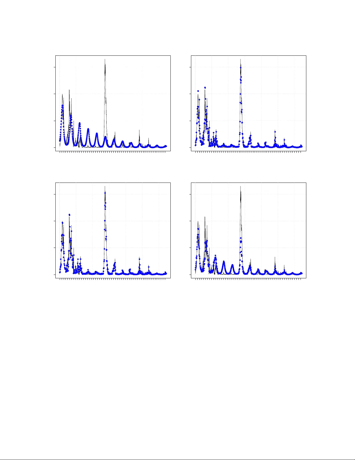
Generalised Linear Mo dels Driv en b y Laten t Pro cesses: Asymptotic Theory and Applications W agner Barreto-Souza ⋆ ∗ and Ngai Hang Chan ♯ † ⋆ Scho ol of Mathematics and Statistics, University Col le ge Dublin, Dublin 4, R epublic of Ir eland ♯ Dep artment of Biostatistics, City University of Hong Kong, Hong Kong F ebruary 19, 2026 Abstract This pap er in tro duces a class of generalised linear mo dels (GLMs) driv en b y la- ten t pro cesses for mo delling coun t, real-v alued, binary , and p ositiv e con tin uous time series. Extending earlier laten t-pro cess regression framew orks based on P oisson or one- parameter exponential family assumptions, w e allo w the conditional distribution of the response to b elong to a bi-parameter exp onen tial family , with the latent pro cess en tering the conditional mean m ultiplicatively . This form ulation substan tially broad- ens the scop e of latent-process GLMs, for instance, it naturally accommo dates gamma resp onses for p ositive con tinuous data, enables estimation of an unkno wn disp ersion parameter via metho d of momen ts, and av oids restrictive conditions on link functions that arise under existing formulations. W e establish the asymptotic normalit y of the GLM estimators obtained from the GLM lik eliho o d that ignores the laten t pro cess, and w e deriv e the correct information matrix for v alid inference. In addition, w e provide a principled approac h to prediction and forecasting in GLMs driv en by latent pro cesses, a topic not previously addressed in the literature. W e presen t tw o real data applica- tions on measles infections in North Rhine-W estphalia (German y) and paleo climatic glacial v arves, which highlight the practical adv antages and enhanced flexibilit y of the prop osed mo delling framework. Keywor ds : Asymptotic inference, Bi-parameter exp onen tial family , Latent pro cess mo d- els, Generalised linear mo dels, Time series regression. ∗ E-mail: wagner.barreto-souza@ucd.ie † E-mail: nhchan@cityu.edu.hk 1 1 In tro duction In a pioneer work, Zeger ( 1988 ) introduced a regression mo del for counts driven b y a w eakly stationary laten t pro cess. Only the t w o first conditional moments (given the laten t pro cess) w ere sp ecified, and a quasi-lik eliho o d estimation pro cedure was considered for in- feren tial purp oses. In a similar vein but assuming a conditional Poisson distribution, Da vis et al. ( 2000 ) explored a P oisson coun t time series { Y t } defined as Y t | ν t ∼ Poisson ( µ t ν t ) , µ t = exp( x ⊤ t β ) , (1) where ν t is a log-normal AR(1) pro cess with mean 1 and some finite v ariance, x t is a v ector of co v ariates, and β is the asso ciated vector of regression co efficients. Among the asymp- totic prop erties explored b y the authors, they established conditions to ensure asymptotic normalit y of the GLM estimators based on the P oisson lik eliho o d b y ignoring the latent pro- cess. The mo del ( 1 ) was also previously studied by Chan & Ledolter ( 1995 ), where a Mon te Carlo EM algorithm w as dev elop ed for estimation of the parameters. A t wo-step estimation pro cedure with the regression parameters b eing estimated from the marginal distribution, and the parameters of the latent pro cess estimated via a comp osite lik eliho o d approac h, was prop osed by Sørensen ( 2019 ). Da vis & W u ( 2009 ) extended mo del ( 1 ) b y replacing the P oisson assumption b y the one- parameter exp onential family (EF), with fo cus on the negativ e binomial case (with kno wn disp ersion parameter). The extended mo del assumes that Y t giv en a stationary strongly mixing latent pro cess ν t follo ws an one-parameter exponential family with conditional mean E ( Y t | ν t ) = h ( x ⊤ t β + ν t ) , (2) where h ( · ) i s the in v erse of a link function suc h that the resulting GLM lik eliho o d is concav e and E ( h ( x ⊤ t β + ν t )) = h ( x ⊤ t β ) . Under th e ab ov e formulation, suc h a function exists, for instance, for Poisson, negativ e binomial, and Gaussian cases. The asymptotic normalit y of the GLM estimators was established based on the GLM lik eliho o d b y ignoring the latent pro cess. Other related recen t con tributions include Maia et al. ( 2021 ), where a class of semipara- metric time series was prop osed by using quasi-likelihoo d mo dels driven b y latent pro cesses, and Barreto-Souza & Ombao ( 2022 ), where a P oisson regression driv en b y a gamma AR(1) pro cess was dev elop ed with a comp osite likelihoo d inferen tial approac h. Our c hief goal in this pap er is to introduce a flexible GLM driven by laten t pro cesses to handle coun ts, real-v alued, contin uous, p ositiv e con tin uous time series. T o do this, we assume that the time series of in terest, sa y { Y t } , conditional on a latent pro cess { ν t } , follo ws a bi-parameter exp onen tial family , with a conditional mean having the latent pro cess in a m ultiplicativ e w a y , and with a disp ersion parameter, whic h can be unkno wn. W e establish the asymptotic normalit y of the GLM estimators and provide the the correct information matrix to assess standard errors of the parameter estimates. Our formulation ha ve some adv an tages when compared to the Da vis & W u ( 2009 )’s mo del as follo ws: (i) by entering 2 the laten t effect in a multiplicativ e w a y instead of additive like in ( 2 ), it allows us to handle a gamma time series to address p ositive con tinuous time series, which is not feasible under the existing approac h (more details on that are provided in Remark 2.1 ); (ii) we consider a disp ersion parameter that can b e estimated based on the method of momen ts, so adding more flexibility; (iii) if the function h ( · ) is not exp onential, then a m ultiplicativ e latent effect form is not p ossible and therefore it is hard to ensure the requiremen ts b y Davis & W u ( 2009 ) to establish the asymptotics for the GLM estimators suc h as E ( h ( x ⊤ t β + ν t )) = h ( x ⊤ t β ) and their condition stated in Theorem 3 (w eak conv ergence of their C n ( s ) quan tit y); under our form ulation, these issues are easily addressed; (iv) w e also address how to predict based on GLMs driven b y laten t pro cesses, whic h is not addressed in the current literature; (v) w e consider differen t latent pro cesses in our numerical results, while a log-normal AR(1) assumption has b een usually adopted in the literature; for example, our empirical illustrations sho w that a gamma AR(1) latent pro cess might provide b etter results when compared to the log-normal AR(1) pro cess. This pap er is organised as follo ws. Section 2 introduces our class of GLMs driven by latent pro cesses and pro vide some basic results. Section 3 establishes the asymptotic normalit y of the GLM estimators based on the Cen tral Limit Theorem for strongly mixing pro cesses by P eligrad and Utev ( 1997 ), and explicitly provide the correct information matrix to assess the standard errors for v alid inference. Prediction and forecasting are addressed in Section 4 . Section 5 presen ts tw o real data applications on measles infection cases in North Rhine- W estphalia (German y) and paleo climatic glacial v arv es time series, whic h illustrates the P oisson and gamma GLM time series models’ p erformance in practice. Concluding remarks are presented in Section 6 . 2 Mo del sp ecification W e start this section b y in tro ducing k ey ingredients to define our class of generalised linear mo dels driven b y laten t pro cesses. Consider a random v ariable Y with distribution b elonging to the exp onen tial family (EF) and density/probabilit y function giv en by π ( y ) = exp  θ y − b ( θ ) ϕ + c ( y ; ϕ )  , y ∈ S , where b ( · ) is assumed to b e t wice differentiable, θ is a real-v alued parameter, ϕ > 0 is a disp ersion parameter, and S is the supp ort of the distribution. It is well-kno w from the EF theory that µ ≡ E ( Y ) = b ′ ( θ ) and V ar ( Y ) = ϕb ′′ ( θ ) = ϕV ( µ ) , where b ′ ( · ) and b ′′ ( · ) denote resp ectiv ely the first and second order deriv atives of b ( · ) , and V ( · ) denotes the v ariance function. The parameter θ can b e expressed in terms of µ , sa y θ = g ( µ ) . W e will also adopt the follo wing notation Y ∼ EF ( µ, ϕ ) . W e now describ e the latent stationary and strongly mixing pro cesses that will b e considered in our n umerical experiments. Log-normal AR(1) . Define { ν t } t ∈ N b y ν t = exp( Z t ) , where { Z t } t ∈ N b e an AR(1) pro- 3 cess with N ( − σ 2 / 2 , σ 2 ) marginals and AR parameter ρ ∈ ( − 1 , 1) . Then, ν t has log-normal marginals, E ( ν t ) = 1 , V ar ( ν t ) = exp( σ 2 ) − 1 , and corr ( ν t + l , ν t ) = exp( σ 2 ρ l ) − 1 exp( σ 2 ) − 1 , for l ≥ 1 . Gamma AR(1) . The sequence { ν t } t ∈ N follo ws a gamma AR(1) (in short GAR) pro cess b y Sim ( 1990 ) with mean 1 and v ariance σ 2 > 0 if the conditional densit y function of ν t giv en ν t − 1 is given b y f ( ν t | ν t − 1 ) = 1 σ 2 (1 − ρ )  ν t ρν t − 1  σ − 2 − 1 2 exp  − ν t + ρν t − 1 σ 2 (1 − ρ )  I σ − 2 − 1  2 √ ρν t ν t − 1 σ 2 (1 − ρ )  , (3) where ρ ∈ (0 , 1) controls the time dep endence, and I u ( x ) = ∞ X k =0 ( x/ 2) 2 k + u Γ( k + u + 1) k ! is the mo d- ified Bessel function of the first kind of order u ∈ R . Also, the GAR pro cess is strictly stationary having gamma marginal distributions with shap e and scale parameters equal to σ − 2 , and autocorrelation function giv en by corr ( ν t + l , ν t ) = ρ l , for l ≥ 1 . Squared AR CH(1) . Let { Z t } t ∈ N b e an AR CH(1) process ( Engle , 1982 ), that is Z t = q ω + ρZ 2 t − 1 ϵ t , (4) where ω > 0 , ρ ∈ (0 , 1) , and { ϵ t } t ∈ N iid ∼ N (0 , 1) . Define the squared ARCH(1) process by ν t = Z 2 t , for t ∈ N , with E ( ν t ) = 1 . This will giv e us that ω = 1 − ρ and will b e in force for what follows. This condition will later ensure that the mo del parameters can b e con- sisten tly estimated. Moreo ver, we assume ρ ∈ (0 , 1 / √ 3) so that the second momen t of ν t is finite and giv en by E ( ν 2 t ) = 3 1 − ρ 2 1 − 3 ρ 2 . In this case, the auto correlation function of ν t is corr ( ν t + l , ν t ) = ρ l , for l ≥ 1 . All ingredients hav e b een established to define the mo del. Let { ν t } t ∈ N b e a latent pro- cess with E ( ν t ) = 1 and E ( ν 2 t ) < ∞ . W e consider a time series { Y t } t ∈ N with conditional distribution given { ν t } t ∈ N b elonging to the exp onen tial family: Y t | ν t ∼ EF ( µ t ν t , ϕ ) , (5) with µ t ≡ h ( x ⊤ nt β ) , (6) where h ( · ) is the in v erse of a canonical link function, x n t is a p × 1 vector of co v ariates that migh t dep end on the sample size n , β is its asso ciated co efficien t vector with dimension p × 1 , and ϕ > 0 is a disp ersion/precision parameter. 4 Remark 2.1. Our formulation ( 5 ) and ( 6 ) is differ ent fr om that c onsider e d by Davis & W u ( 2009 ) (se e Equation 2 ). W e enter the latent pr o c ess into the mo del in a multiplic ative way. Our formulation and Davis & W u ( 2009 ) ones wil l c oincide only when the lo g link function is c onsider e d. Under ( 5 ) and ( 6 ), we ar e able to hand le c ontinuous p ositive time series b ase d on, for example, the gamma and inverse Gaussian distributions sinc e the c onditions on the link function describ e d b elow Equation ( 2 ) ar e satisfie d. On the other hand, such c onditions for the gamma and inverse Gaussian c ases ar e c omplic ate d (if not imp ossible) to b e che cke d under the formulation by Davis & W u ( 2009 ). The exp ected v alue of our time series is E ( Y t ) = E [ E ( Y t | ν t )] = h ( x ⊤ nt β ) E ( ν t ) = h ( x ⊤ nt β ) = µ t since w e are imp osing that E ( ν t ) = 1 . By assuming that the v ariance function of the GLM assumes the form V ( µ ) = µ γ , for γ ≥ 0 , and that E ( ν max( γ , 2) t ) < ∞ , we obtain that the v ariance of Y t is V ar ( Y t ) = E [ V ar ( Y t | ν t )] + V ar [ E ( Y t | ν t )] = E [ ϕV ( µ t ν t )] + V ar ( µ t ν t ) = ϕµ γ t E ( ν γ t ) + µ 2 t V ar ( ν t ) = ϕµ γ t κ γ + µ 2 t ( κ 2 − 1) , where κ j ≡ E ( ν j t ) for j > 0 . F or l ∈ N , the co v ariance function is co v ( Y t + l , Y t ) = co v ( E ( Y t + l | ν t + l ) , E ( Y t | ν t )) + E ( cov ( Y t + l , Y t | ν t + l , ν t )) = µ t + l µ t co v ( ν t + l , ν t ) + 0 = µ t + l µ t co v ( ν t + l , ν t ) , and the autocorrelation function assumes the form corr ( Y t + l , Y t ) = µ t + l µ t co v ( ν t + l , ν t ) q [ ϕµ γ t + l κ γ + µ 2 t + l ( κ 2 − 1)][ ϕµ γ t κ γ + µ 2 t ( κ 2 − 1)] . Explicit expressions for the v ariance and auto cov ariance/auto correlation function of Y t are obtained by using the momen ts and auto cov ariance/auto correlation function of the latent pro cesses describ ed abov e. 3 Asymptotic distribution of the GLM estimators W e now establish the asymptotic distribution of the estimators based on a GLM pseudo log-lik eliho o d function for the GLMs driv en b y latent processes. The estimation of ϕ and the parameters related to the latent pro cess will b e p erformed via metho d of moments and will b e illustrated in our real data applications in Section 5 . The pseudo log-likelihoo d function under a GLM with canonical link function (hence 5 θ t = g ( x ⊤ n t β ) = x ⊤ n t β ) is giv en b y ℓ ( β ) = n X t =1  [ x ⊤ nt β Y t − b ( x ⊤ nt β )] /ϕ + c ( Y t ; ϕ )  . The GLM estimator of β , sa y b β , is obtained by b β = argmax β ℓ ( β ) , which do es not dep end on ϕ . Since the canonical link function is considered, ℓ ( · ) is conca v e, and this ensures the existence and uniqueness of b β . T o show the asymptotic normality of the GLM estimators, w e start b y s ho wing the asymptotic normality of the quan tity n − 1 / 2 n X t =1 x nt µ 0 t ( ν t − 1) , (7) whic h is a key result to establish the asymptotic distribution of √ n ( b β − β 0 ) , where β 0 is the true v alue of β and µ 0 t = h ( x ⊤ nt β 0 ) . T o do this, we need the definition of α -mixing (strongly mixing) pro cesses and a Cen tral Limit Theorem (CL T) by P eligrad and Utev ( 1997 ). Definition 3.1. [ α -mixing] L et { X t } t ∈ N b e a stationary pr o c ess and denote the σ -algebr a F m n = σ ( X n , X n +1 , . . . , X m ) , for n ≤ m . Define α ( n ) = sup k sup A ∈F k 1 ,B ∈F ∞ k + n | P ( A ∩ B ) − P ( A ) P ( B ) | . W e say that { X t } t ∈ N is α -mixing (str ongly mixing) if α ( n ) → 0 as n → ∞ . Let { a nt } n,t ∈ N b e a triangular array of real n umbers. Theorem 2.2(c) from Peligrad and Utev ( 1997 ) states that a centred sto chastic sequence { ζ t } t ∈ N satisfies the w eak conv ergence n X t =1 a nt ζ t d − → N (0 , 1) as n → ∞ if the following conditions hold: (C1) { ζ t } t ∈ N is strongly mixing, and for certain δ > 0 , {| ζ t | 2+ δ } t ∈ N is uniformly in tegrable, inf t V ar ( ζ t ) > 0 and ∞ X t =1 t 2 /δ α ( t ) < ∞ ; (C2) { ζ 2 t } t ∈ N is an uniformly in tegrable family and V ar n X t =1 a nt ζ t ! = 1 ; and (C3) sup n n X t =1 a 2 nt < ∞ and max 1 ≤ t ≤ n | a nt | → 0 as n → ∞ . W e also need to imp ose some conditions on the cov ariates to derive the asymptotic prop- erties for the GLM estimators. The conditions below ha v e b een considered b y Davis et al. ( 2000 ) and Da vis & W u ( 2009 ). Assumptions on cov ariates. Denote by β 0 the true v alue of β and µ t ≡ h ( x ⊤ nt β 0 ) . 6 There exists a non-singular matrix Ω I suc h that lim n →∞ n − 1 n X t =1 x nt x ⊤ nt V ( µ 0 t ) ≡ Ω I . (8) There exists a matrix Ω † I suc h that the follo wing conv ergence in probabilit y holds as n → ∞ : n − 1 n X t =1 x nt x ⊤ nt V ( µ 0 t ν t ) p − → Ω † I . (9) As n → ∞ , we assume that n − 1 n X t =1 x nt x ⊤ nt µ 0 t µ 0 t + l − → W l , (10) uniformly in | l | < n , n − 1 − l X t =1 x nt x ⊤ nt µ 0 t µ 0 t + l − → 0 , (11) for each l < 0 , and n − 1 n X t = n − l +1 x nt x ⊤ nt µ 0 t µ 0 t + l − → 0 , (12) for each l > 0 . F urthermore, it is assumed that left-hand sides of ( 11 ) and ( 12 ) are uniformly b ounded in l ∈ ( − n, 0) and l ∈ (0 , n ) , resp ectively , as n → ∞ . The last assumption on the co v ariates is that sup 1 ≤ t ≤ n n − 1 / 2 | x nt µ 0 t | → 0 , (13) as n → ∞ . In the next theorem, we pro vide the asymptotic distribution of ( 7 ). Theorem 3.1. Assume that { ν t } t ∈ N is a sto chastic pr o c ess satisfying (C1) and that the assumptions on c ovariates ( 10 )-( 13 ) hold. Then, the fol lowing asymptotic normality i s valid: n − 1 / 2 n X t =1 x nt µ 0 t ( ν t − 1) d − → N ( 0 , Ω I I ) , as n → ∞ , wher e β 0 denotes the true value of β and Ω I I = ∞ X l = −∞ γ ν ( l ) W l , with γ ν ( · ) b eing the auto c ovarianc e function of ν t . 7 Pr o of. Define C n ( s ) = s ⊤ n − 1 / 2 n X t =1 x nt µ 0 t ( ν t − 1) and τ 2 n ( s ) = V ar ( C n ( s )) . It follows that τ 2 n ( s ) = s ⊤ n − 1 n X t =1 n X k =1 x nt µ 0 t x ⊤ nk µ 0 k co v ( ν t , ν k ) s = s ⊤ n − 1 n X t =1 n X k =1 x nt x ⊤ nk µ 0 t µ 0 k γ ν ( t − k ) s , By making a c hange of index l = t − k and using Assumptions ( 10 ), ( 11 ), and ( 12 ), we obtain that lim n →∞ τ 2 n ( s ) = s ⊤ ∞ X l = −∞ γ ν ( l ) W l s = s ⊤ Ω I I s . W e now define ζ t = ν t − 1 and a nt = 1 τ n ( s ) n − 1 / 2 s ⊤ x nt µ 0 t . Condition (C1) from the CL T for strongly mixing processes ( P eligrad and Utev , 1997 ) is a hypothesis of our theorem. Also, V ar n X t =1 a nt ζ t ! = 1 τ 2 n ( s ) V ar ( C n ( s )) = 1 τ 2 n ( s ) τ 2 n ( s ) = 1 . Therefore, Condition (C2) is satisfied. Moreov er, n X t =1 a 2 nt = 1 τ 2 n ( s ) s ⊤ n − 1 n X t =1 x nt x ⊤ nt ( µ 0 t ) 2 s − → s ⊤ W 0 s s ⊤ Ws , as n → ∞ , and max 1 ≤ t ≤ n | a nt | = 1 τ n ( s ) max 1 ≤ t ≤ n | s ⊤ n − 1 / 2 x nt µ 0 t | ≤ 1 τ n ( s ) | s | ⊤ max 1 ≤ t ≤ n n − 1 / 2 | x nt µ 0 t | − → 0 , as n → ∞ , where w e used that lim n →∞ τ n ( s ) = √ s ⊤ Ws and Assumption ( 13 ) to obtain the null limit. These results giv e us that Condition (C3) holds. Since all conditions from Theorem 2.2(c) from P eligrad and Utev ( 1997 ) hold, we obtain the claimed asymptotic normalit y . Theorem 3.2. Supp ose that { ν t } t ∈ N is a sto chastic pr o c ess satisfying (C1) and that the c ovariates satisfy Assumptions ( 8 )-( 13 ). Then, the GLM estimator of β is c onsistent and satisfies the asymptotic normality √ n  b β − β 0  d − → N  0 , Ω − 1 I ( ϕ Ω † I + Ω I I ) Ω − 1 I  , as n → ∞ , wher e β 0 denotes the true value of β . Pr o of. F ollo wing a similar strategy b y Davis et al. ( 2000 ) and Davis & W u ( 2009 ), we define 8 u ≡ √ n ( β − β 0 ) and g n ( u ) ≡ − ϕ { ℓ ( β ) − ℓ ( β 0 ) } , where β 0 is the true parameter v ector. Under this formulation, the GLM estimator is obtained b y minimising g n ( u ) with resp ect to β . Also, β = n − 1 / 2 u + β 0 . It follows that g n ( u ) = − ϕ { ℓ ( n − 1 u + β 0 ) − ℓ ( β 0 ) } = n X t =1  x ⊤ nt β 0 Y t − b ( x ⊤ nt β 0 ) − x ⊤ nt ( n − 1 / 2 u + β 0 ) Y t + b  x ⊤ nt ( n − 1 / 2 u + β 0 )  = n X t =1  − x ⊤ nt n − 1 / 2 u Y t + b  x ⊤ nt ( n − 1 / 2 u + β 0 )  − b ( x ⊤ nt β 0 )  . W e ha ve that n X t =1  b  x ⊤ nt ( n − 1 / 2 u + β 0 )  − b ( x ⊤ nt β 0 )  ≈ n X t =1  x ⊤ nt n − 1 / 2 u b ′ ( x ⊤ nt β 0 ) + ( x ⊤ nt n − 1 / 2 u ) 2 2 b ′′ ( x ⊤ nt β 0 )  = n X t =1  x ⊤ nt n − 1 / 2 u µ 0 t + ( x ⊤ nt n − 1 / 2 u ) 2 2 V ( µ 0 t )  , where w e ha v e defined µ 0 t ≡ h ( x ⊤ nt β 0 ) , and V ( µ 0 t ) ≡ b ′′ ( x ⊤ nt β 0 ) denotes the v ariance function from GLMs. It follo ws that g n ( u ) p ≈ − n − 1 / 2 n X t =1 x ⊤ nt u ( Y t − µ 0 t ) + 1 2 u ⊤ n − 1 n X t =1 x nt x ⊤ nt V ( µ 0 t ) ! u . (14) F rom Assumption ( 8 ), the second term on the righ t side of ( 14 ) conv erges to 1 2 u ⊤ Ω I u as n → ∞ . W e will no w establish the asymptotic normality of Q n ≡ n − 1 / 2 n X t =1 ( Y t − µ 0 t ) x nt . F or a real vector s , the conditional c haracteristic function of Q n giv en ν t is E  exp { i s ⊤ Q n }| ν t  = exp ( − i s ⊤ n − 1 / 2 n X t =1 µ 0 t x nt ) E exp ( − i s ⊤ n − 1 / 2 n X t =1 Y t x nt )    ν t ! , where w e use the mo del sp ecification Y t | ν t ∼ EF ( µ t ν t , ϕ ) and the notation e θ t = g ( µ t ν t ) to 9 obtain that E exp ( − i s ⊤ n − 1 / 2 n X t =1 Y t x nt )    ν t ! = exp ( ϕ − 1 n X t =1 h b ( e θ t + iϕn − 1 / 2 s ⊤ x nt ) − b ( e θ t ) i ) p ≈ exp ( ϕ − 1 n X t =1  i s ⊤ x nt n − 1 / 2 ϕb ′ ( e θ t ) + ( i s ⊤ x nt n − 1 / 2 ϕ ) 2 2 b ′′ ( e θ t )  ) = exp ( i s ⊤ n − 1 / 2 n X t =1 x nt µ 0 t ν t − 1 2 ϕ s ⊤ n − 1 n X t =1 x nt x ⊤ nt V ( µ 0 t ν t ) ! s ) . Hence, we obtain that E  exp { i s ⊤ Q n }| ν t  p ≈ exp ( i s ⊤ n − 1 / 2 n X t =1 x nt µ 0 t ( ν t − 1) − 1 2 ϕ s ⊤ n − 1 n X t =1 x nt x ⊤ nt V ( µ 0 t ν t ) ! s ) . F rom Theorem 3.1 , n − 1 / 2 n X t =1 x nt µ 0 t ( ν t − 1) d → F ∼ N ( 0 , Ω I I ) , and from Assumption 9 n − 1 n X t =1 x nt x ⊤ nt V ( µ 0 t ν t ) p − → Ω † I . Hence, lim n →∞ E  exp { i s ⊤ Q n }  = E  exp  i s ⊤ F − 1 2 ϕ s ⊤ Ω † I s  = exp  − 1 2 s ⊤  ϕ Ω † I + Ω I I  s  , that is Q n d → Q ∼ N ( 0 , ϕ Ω † I + Ω I I ) . This implies that g n ( u ) d → − u ⊤ Q + 1 2 u ⊤ Ω I u . Arguing similarly as in Da vis & W u ( 2009 ), the limit process of g n ( u ) has a unique minimiser, say e u , and √ n  b β − β 0  d − → e u ∼ N  0 , Ω − 1 I ( ϕ Ω † I + Ω I I ) Ω − 1 I  . 4 Prediction and forecasting W e here prop ose to p erform prediction or forecasting based on the conditional exp ectation E ( Y t + h | Y t ) . Although our prop osed GLM time series are not Mark o vian, this can b e used for prediction purp oses. Suc h approac h has b een successfully emplo y ed in non-Mark o vian mo dels; for instance, see Maia et al. ( 2021 ) and Barreto-Souza & Om bao ( 2022 ). F ollo wing similar arguments as in those pap ers, for l ≥ 1 , w e obtain that E ( Y t + l | Y t ) = E [ E ( Y t + l | ν t ) | Y t ] , (15) 10 with E ( Y t + l | ν t ) = E [ E ( Y t + l | ν t + l ) | ν t ] = µ t + l E ( ν t + l | ν t ) . W e will now pro vide explicit expres- sions for ( 15 ) for the three latent pro cesses considered in this pap er. Under a log-normal AR(1) pro cess, it follo ws that E ( ν t + l | ν t ) = exp( ρ l σ 2 (1 − ρ l ) / 2 + ρ l log ν t ) . Hence, E ( Y t + l | Y t ) = µ t + l exp( ρ l σ 2 (1 − ρ l ) / 2) E [exp( ρ l log ν t ) | Y t )] , with E [exp( ρ l log ν t ) | Y t )] = Z ∞ 0 exp( ρ l log ν ) f y t | ν t ( y | ν ) f ν t ( ν ) dν Z ∞ 0 f y t | ν t ( y | ν ) f ν t ( ν ) dν , whic h can b e computed n umerically , where f y t | ν t ( ·|· ) and f ν t ( ν ) are EF and log-normal density functions, resp ectively . F or ν t ∼ GAR (1) , we hav e that E ( ν t + l | ν t ) = 1 + ρ l ( ν 1 − 1) (for instance, see Barreto-Souza & Ombao ( 2022 )), and therefore E ( Y t + l | Y t ) = µ t + l { 1 + ρ l [ E ( ν t | Y t ) − 1] } . (16) The conditional expectation on the right side of ( 16 ) can b e computed explicitly for some sp ecial cases. Let us consider the P oisson and gamma GLMs. F or the P oisson sce- nario, w e can sho w that the conditional distribution of ν t giv en Y t follo ws a gamma dis- tribution with shap e and rate parameters y t + 1 /σ 2 and µ t + 1 /σ 2 , resp ectively , which giv es us that E ( ν t | Y t ) = y t + 1 /σ 2 µ t + 1 /σ 2 . Under the gamma setup, it can b e shown that the conditional distribution of ν t | Y t follo ws a generalised inv erse Gaussian distribution with parameters a = 2 /σ 2 , b t = 2 y t µ t ϕ , and p = 1 /σ 2 − 1 /ϕ , with densit y function assuming the form f ν t | Y t ( ν t | y t ) = ( a/b t ) p/ 2 2 K p ( √ ab t ) ν p − 1 t exp {− ( aν t + b t /ν t ) / 2 } , for ν t > 0 , where K p ( u ) = 1 2 Z ∞ 0 ω p − 1 exp  − u 2  ω + 1 ω  dω is the mo dified Bessel function of third kind for u > 0 and p ∈ R . Using this result, it follows that E ( ν t | Y t ) = s σ 2 y t ϕµ t K 1 /σ 2 − 1 /ϕ +1  2 r y t σ 2 ϕµ t  K 1 /σ 2 − 1 /ϕ  2 r y t σ 2 ϕµ t  . No w, consider the AR CH(1) laten t process. Then, E ( ν t + l | ν t ) = 1 + ρ l ( ν t − 1) , and therefore the conditional exp ectation E ( Y t + l | Y t ) assumes the form ( 16 ). In this case, closed- forms expressions for the conditional exp ectation on the righ t side of ( 16 ) cannot b e obtained, 11 but they can b e computed apro ximately via Mon te Carlo sim ulation. W e hav e that E ( ν t | Y t ) = Z ∞ 0 ν t f y t | ν t ( y t | ν t ) f ν t ( ν t ) dν t Z ∞ 0 f y t | ν t ( y t | ν t ) f ν t ( ν t ) dν t = E ν t  ν t f y t | ν t ( y t | ν t )  E ν t  f y t | ν t ( y t | ν t )  , where the underscript in E ν t ( · ) means that the expected v alue is tak en with resp ect to ν t . Hence, we generate m dra ws from ARCH tra jectories { ν ( i ) t } n t =1 ( i = 1 , . . . , m ) and appro ximate the conditional exp ectations by their Monte Carlo estimates b E ( ν t | Y t ) = m − 1 m X k =1 ν ( k ) t f y t | ν t ( y t | ν ( k ) t ) m − 1 m X k =1 f y t | ν t ( y t | ν ( k ) t ) , for t = 1 , . . . , n . The metho dology prop osed here for prediction will b e illustrated in the real data applications in Section 5 . 5 Real data analyses W e here present tw o real data applications to show the performance of our GLM time series mo dels in practice to handle coun ts and positive con tin uous data. 5.1 Measles infections in North Rhine-W estphalia (German y) Let us consider the weekly n um b er of measles infections rep orted in North Rhine-W estphalia (German y) from Jan uary 2001 to May 2013, so totaling 646 observ ations. The data is pub- licly a v ailable in the R pack age tscount . The plot of the measles time series and its ACF are display ed in Figure 1 . The follo wing vector of cov ariates, including trend and seasonal comp onen ts, are considered: x t = (1 , t/ 646 , cos(2 π t/ 52) , sin(2 π t/ 52) , cos(4 π t/ 52) , sin(4 π t/ 52) , cos(8 π t/ 52) , sin(8 π t/ 52)) ⊤ , for t = 1 , . . . , 646 . T able 1 provides a summary of the GLM fitting with the resp ectiv e standard errors. The estimation of the parameters σ 2 and ρ of the Poisson LNAR(1) mo del are obtained through the metho d of momen t pro cedure: b σ 2 = log  P n t =1 [( Y t − b µ t ) 2 − b µ t ] P n t =1 b µ 2 t + 1  , b ρ = log  P n t =1 ( Y t − b µ t )( Y t − 1 − b µ t − 1 ) P n t =2 b µ t b µ t − 1 + 1   b σ 2 , 12 0 50 100 150 Time Reported measles cases 2001 2001 2002 2003 2004 2005 2006 2007 2008 2009 2010 2011 2012 2012 0 10 20 30 40 50 60 0.0 0.2 0.4 0.6 0.8 Lag ACF Figure 1: Plots of the w eekly rep orted cases of measles in North Rhine-W estphalia, Germany , b et w een January 2001 and May 2013 and its resp ectiv e auto correlation function. b µ t = h ( x ⊤ nt b β ) , with b β b eing the GLM estimator of β . In this case, the estimates are b σ 2 = 0 . 751 and b ρ = 0 . 924 . As for the P oisson GAR(1) mo del, the metho d of moments estimators of σ 2 and ρ assume the form b σ 2 = P n t =1 [( Y t − b µ t ) 2 − b µ t ] P n t =1 b µ 2 t , b ρ = P n t =1 ( Y t − b µ t )( Y t − 1 − b µ t − 1 ) b σ 2 P n t =2 b µ t b µ t − 1 , whic h yield the estimates b σ 2 = 1 . 118 and b ρ = 0 . 895 . Under the Poisson AR CH(1) mo del, to estimate the parameter ρ , w e use the first-order auto correlation of Y t to obtain the metho d of moments estimator b ρ as the solution of the nonlinear equation b ρ  3(1 − b ρ 2 ) 1 − 3 b ρ 2 − 1  = n − 1 X t =1 ( Y t − b µ t )( Y t +1 − b µ t +1 ) / n − 1 X t =1 b µ t b µ t +1 , The metho d of momen ts estimate of ρ is b ρ = 0 . 333 , which b elongs to the in terv al (0 , 1 / √ 3) . Therefore, the theoretical results obtained in this pap er can b e applied to analyze the measles time series. T o obtain the standard errors under the Poisson case ( V ( µ ) = µ ), we use the fact that E ( ν t ) = 1 and hence b oth Ω I and Ω † I can b e consistently estimated b y b Ω I = b Ω † I = n − 1 n X t =1 x nt x ⊤ nt b µ t , while b Ω I I = n − 1 n X t =1 n X k =1 x nt x ⊤ nk b µ t b µ k b γ ν ( | t − k | ) is a consisten t estimator for 13 Ω I I , where b γ ν ( · ) is a consisten t estimator of γ ν ( · ) . In addition, a parametric b o otstrap with 1000 replications is also employ ed to obtain the standard errors and the related results are also presen ted in T able 1 . As exp ected, the GLM approac h do es not pro vide correct standard errors as it ignores the temp oral dep endence. As a consequence, w e notice the difference b etw een such a quan tity provided under GLM and b o otstrap approac h, whic h is line with the n umerical exp eriments by Da vis et al. ( 2000 ) and Davis & W u ( 2009 ). Only the cov ariate sin(8 π t/ 52) is not significant according to GLM-based inference at a significance lev el at 5%. On the other hand, the co v ariates cos(4 π t/ 52) , sin(4 π t/ 52) , cos(8 π t/ 52) , and sin(8 π t/ 52) are not significan t based on the parametric bo otstrap method, where a normal appro ximation was considered, which is in line with the inference based on correct information matrix, where the temp oral dep endence is taken in to accoun t. estimates β 0 β 1 β 2 β 3 β 4 β 5 β 6 β 7 GLM 3.043 − 3.370 − 0.683 1.108 − 0.054 − 0.083 − 0.040 − 0.012 Bo ot. LNAR 2.947 − 3.296 − 0.675 1.108 − 0.054 − 0.079 − 0.037 − 0.011 Bo ot. GAR 2.861 − 3.145 − 0.728 1.070 − 0.078 − 0.095 − 0.037 − 0.022 Bo ot. ARCH 2.962 − 3.328 − 0.684 1.108 − 0.066 − 0.078 − 0.035 − 0.007 stand. error β 0 β 1 β 2 β 3 β 4 β 5 β 6 β 7 GLM 0.025 0.057 0.027 0.029 0.023 0.023 0.019 0.019 LNAR 0.441 0.981 0.216 0.221 0.148 0.150 0.097 0.097 Bo ot. LNAR 0.391 0.879 0.194 0.201 0.129 0.130 0.084 0.082 GAR 0.418 0.946 0.225 0.229 0.153 0.155 0.098 0.098 Bo ot. GAR 0.378 0.821 0.220 0.224 0.147 0.157 0.102 0.095 AR CH 0.248 0.604 0.185 0.182 0.207 0.205 0.214 0.214 Bo ot. ARCH 0.212 0.534 0.171 0.164 0.188 0.185 0.194 0.185 T able 1: P arameter estimates based on GLM, b o otstrap, and their resp ective standard errors for the measles time series. T o ev aluate the predictiv e p erformance of the models, we compute the ro ot mean square error (RMSE) based in-sample forecasting. T able 2 pro vides the RMSE and the correlation b et w een predictions and observ ations for the mo dels considered here. In-sample forecasting for the weekly rep orted cases of measles based on GLM, GLM-LNAR, GLM-GAR, and GLM- AR CH along with the observ ed time series are displa y ed in Figure 2 . These results sho w that GLM-LNAR and GLM-GAR yield go o d results in terms of prediction with a b etter p erformance for the GLM-based on the GAR latent pro cess. 5.2 P aleo climatic glacial v arv es The second real data application is ab out the ticknesses of the yearly sedimentary dep osits (v arves) from one lo cation in Massach usetts (ab out 12,600 y ears ago) for 634 y ears. V arv es can b e used as pro xies for paleo climatic parameters, for instance, to reconstruct past climates 14 Mo del → GLM GLM-LNAR GLM-GAR GLM-ARCH RMSE 17.761 8.837 8.724 12.893 Correlation 0.582 0.914 0.917 0.820 T able 2: RMSE and correlation b etw een observ ations and their resp ective in-sample predic- tions under GLM, GLM-LNAR, GLM-GAR, and GLM-ARCH for the measles time series data analysis. and other en vironmen tal changes. F or more details, see Example 2.6 from the b o ok by Sh um w ay and Stoffer ( 2011 ). A plot of the v arve time series and its A CF are provided in Figure 3 . W e consider a gamma GLM (with an in v erse canonical link function) driv en by laten t pro cesses and v ector of co v ariates with a trend: x t = (1 , t/ 634) ⊤ , for t = 1 , . . . , 634 . The summary fit of the gamma GLM under LNAR(1), GAR(1), and AR CH(1) laten t pro cesses are provided in T able 3 . T o estimate the disp ersion ϕ parameters of the latent pro cesses, we use metho d of momen ts. Under LNAR(1), w e use the estimators b ρ = log  P n t =3 ( Y t − b µ t )( Y t − 2 − b µ t − 2 ) P n t =3 b µ t b µ t − 2 + 1   log  P n t =2 ( Y t − b µ t )( Y t − 1 − b µ t − 1 ) P n t =2 b µ t b µ t − 1 + 1  , b σ 2 = log 2  P n t =2 ( Y t − b µ t )( Y t − 1 − b µ t − 1 ) P n t =2 b µ t b µ t − 1 + 1   log  P n t =3 ( Y t − b µ t )( Y t − 2 − b µ t − 2 ) P n t =3 b µ t b µ t − 2 + 1  , b ϕ = exp( − b σ 2 )  P n t =1 ( Y t − b µ t ) 2 P n t =1 b µ 2 t + 1  − 1 , whic h yield the parameter estimates b ρ = 0 . 881 , b σ 2 = 0 . 297 , and b ϕ = 0 . 123 . As for the GAR(1) latent pro cess, we ha ve the estimators b ρ = P n t =3 ( Y t − b µ t )( Y t − 2 − b µ t − 2 ) P n t =2 ( Y t − b µ t )( Y t − 1 − b µ t − 1 ) P n t =2 b µ t b µ t − 1 P n t =3 b µ t b µ t − 2 , b σ 2 =  P n t =2 ( Y t − b µ t )( Y t − 1 − b µ t − 1 ) P n t =2 b µ t b µ t − 1  2 P n t =3 b µ t b µ t − 2 P n t =3 ( Y t − b µ t )( Y t − 2 − b µ t − 2 ) , b ϕ = ( b σ 2 + 1) − 1  P n t =1 ( Y t − b µ t ) 2 P n t =1 b µ 2 t + 1  − 1 , with the parameter estimates b ρ = 0 . 867 , b σ 2 = 0 . 345 , and b ϕ = 0 . 123 . In this application, w e do not consider the ARCH latent pro cess since that the MM estimator of ϕ yielded a negativ e v alue. W e can notice a go o d agreemen t b etw een the GLM and b o otstrap estimates and standard errors (under our formulation) as w ell. By ignoring the dep endence on the data, the trend is statistically significan t, whic h is conflitant with the conclusion based on the mo delling taking into accoun t dep endence, where this co v ariate is not significant. T able 4 rep orts the RMSE and correlation b etw een observ ations and their resp ective in-sample predictions under GLM, GLM-LNAR, and GLM-GAR for the v arve time series. 15 0 50 100 150 GLM Time Repor ted measles cases 2001 2002 2003 2005 2006 2007 2009 2010 2012 0 50 100 150 GLM−LNAR Time Repor ted measles cases 2001 2002 2003 2005 2006 2007 2009 2010 2012 0 50 100 150 GLM−GAR Time Repor ted measles cases 2001 2002 2003 2005 2006 2007 2009 2010 2012 0 50 100 150 GLM−ARCH Time Repor ted measles cases 2001 2002 2003 2005 2006 2007 2009 2010 2012 Figure 2: In-sample forecasting (dots) for the weekly rep orted cases of measles based on GLM, GLM-LNAR, GLM-GAR, and GLM-AR CH along with the observed time series (solid line). GLM-LNAR and GLM-GAR pro duce the b est and similar results, with slight adv antage for the latter. Plots of the in-sample predictions based on GLM, GLM-LNAR, and GLM-GAR are presented in Figure 4 , which sho ws a go o d p erformance of the prediction methodology of our models proposed in Section 4 . 16 Time V arve 0 100 200 300 400 500 600 0 50 100 150 0 10 20 30 40 0.0 0.2 0.4 0.6 0.8 1.0 Lag ACF Figure 3: Plots of the v arve time series and its resp ective auto correlation function. estimates β 0 β 1 GLM 0.044 − 0.016 Bo ot. LNAR 0.045 − 0.016 Bo ot. GAR 0.046 − 0.018 stand. error β 0 β 1 GLM 0.002 0.003 LNAR 0.008 0.012 Bo ot. LNAR 0.007 0.011 GAR 0.008 0.012 Bo ot. GAR 0.007 0.011 T able 3: P arameter estimates based on GLM, b o otstrap, and their resp ective standard errors for the v arv e time series. Mo del → GLM GLM-LNAR GLM-GAR RMSE 20.099 16.098 16.065 Correlation 0.148 0.610 0.612 T able 4: RMSE and correlation b etw een observ ations and their resp ective in-sample predic- tions under GLM, GLM-LNAR, and GLM-GAR for the v arv e time series data analysis. 6 Concluding remarks W e prop osed a flexible class of generalised linear mo dels driv en b y laten t pro cesses for mo deling count, real-v alued, contin uous, and p ositive con tinuous time series. By assuming that Y t , conditional on ν t , follo ws a bi-parameter exp onen tial family with a multiplicativ e 17 0 100 200 300 400 500 600 0 50 100 150 GLM time V ar ve 0 100 200 300 400 500 600 0 50 100 150 GLM−LNAR time V ar ve 0 100 200 300 400 500 600 0 50 100 150 GLM−GAR time V ar ve Figure 4: In-sample forecasting (dots) for the v arve time series based on GLM, GLM-LNAR, GLM-GAR, and GLM-AR CH along with the observ ed time series (solid line). laten t effect in the conditional mean, our formulation ov ercomes some limitations of ex- isting approac h es and accommodates imp ortan t cases, suc h as gamma-distributed p ositiv e time series, that are not feasible under the additive laten t structure of Da vis & W u ( 2009 ). The inclusion of an estimable disp ersion parameter and the absence of a strong restriction condition on the link function h ( · ) further enhance model flexibilit y . W e established the asymptotic normalit y of the GLM estimators using the Central Limit Theorem for strongly mixing pro cesses by Peligrad and Utev ( 1997 ) and derived the corre- sp onding information matrix for inference. W e also developed prediction metho ds for GLMs 18 with latent pro cesses, addressing a gap in the literature. Empirical illustrations sho wed that alternative laten t dynamics, such as a gamma AR(1) pro cess, may pro vide improv ed p erformance ov er the commonly used log-normal AR(1). Ov erall, the prop osed framew ork offers a v ersatile and theoretically sound basis for mo delling time series with laten t dynamic structure. A c kno wledgemen ts WBS thanks the Department of Biostatistics from City Univ ersit y of Hong Kong for the w arm hospitality during his research visit, where part of this w ork w as dev elop ed. References Barreto-Souza, W. & Omba o, H. (2022). The negative binomial pro cess: A tractable mo del with comp osite likelihoo d-based inference. Sc andinavian Journal of Statistics . 49 , 568–592. Chan, K.S. & Ledol ter, J. (1995). Mon te Carlo EM algorithm for time series mo dels in v olving counts. Journal of the Americ an Statistic al Asso ciation . 90 , 242-252. D a vis, R.A, Dunsmuir, W.T.M. & W ang, Y. (2000). On auto correlation in a Poisson regression mo del. Biometrika . 87 , 491–505. D a vis, R.A. & Wu, R. (2009). A negative binomial mo del for time series of coun ts. Biometrika . 96 , 735–749. Engle, R.F. (1982). Autoregressiv e conditional heteroskedasticit y with estimates of the v ariance of U.K. inflation. Ec onometric a 50 , 987–1008. Maia, G.O., Barreto-Souza, W., Bastos, F.S. & Omba o, H. (2021). Semiparametric time series mo dels driv en b y latent factor. International Journal of F or e c asting . 37 , 1463– 1479. Sørensen, H. (2019). Indep endence, successive and conditional likelihoo d for time series of counts. Journal of Statistic al Planning and Infer enc e . 200 , 20–31. Peligrad, M. & Utev, S. (1997). Central limit theorem for linear pro cesses. Annals of Pr ob ability . 25 , 443–456. Shumw a y, R.H. & Stoffer, D.S. (2011). Time Series Analysis and Its Applications: With R Examples. Springer, New Y ork, 3rd edition. Sim, C. H. (1990). First-order autoregressiv e mo dels for gamma and exp onen tial pro cesses. Journal of Applie d Pr ob ability . 27 , 325–332. Zeger, S.L. (1988). A regression mo del for time series of counts. Biometrika . 75 , 621–629. 19