Functional Decomposition and Shapley Interactions for Interpreting Survival Models

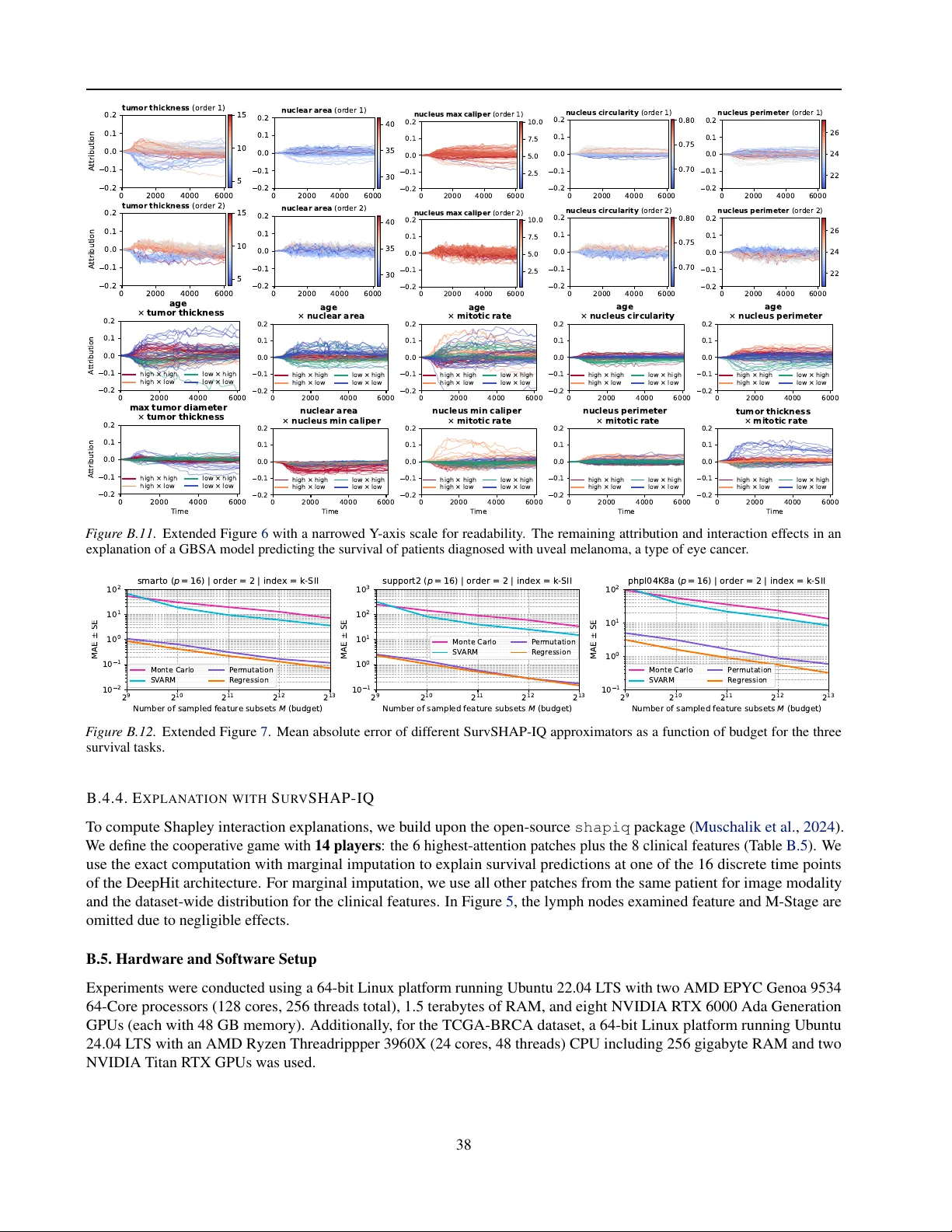
Functional Decomposition and Shapley Interactions f or Interpr eting Survi val Models Sophie Hanna Langbein 1 2 Hubert Baniecki 3 4 Fabian Fumagalli 5 6 Niklas Koenen 1 2 Marvin N. Wright 1 2 Julia Herbinger 1 Abstract Hazard and surviv al functions are natural, inter - pretable targets in time-to-ev ent prediction, but their inherent non-additi vity fundamentally lim- its standard additive e xplanation methods. W e introduce Surviv al Functional Decomposition (SurvFD), a principled approach for analyzing feature interactions in machine learning survi v al models. By decomposing higher-order effects into time-dependent and time-independent com- ponents, SurvFD of fers a pre viously unrecognized perspectiv e on surviv al explanations, explicitly characterizing when and why additive explana- tions fail. Building on this theoretical decompo- sition, we propose SurvSHAP-IQ, which extends Shapley interactions to time-index ed functions, providing a practical estimator for higher -order , time-dependent interactions. T ogether , SurvFD and SurvSHAP-IQ establish an interaction- and time-aware interpretability approach for surviv al modeling, with broad applicability across time-to- ev ent prediction tasks. 1. Introduction Understanding whether effects vary across subgroups, pa- tient characteristics, or co-e xposures is critical for clinical and public health decisions. Such interactions are impor - tant in surviv al analysis, e.g., between genetic and en viron- mental factors ( Minelli et al. , 2011 ), obesity and treatment effects ( Hanai et al. , 2014 ; Jensen et al. , 2008 ), or age and tu- mor markers ( Julkunen & Rousu , 2025 ; Nielsen & Grønbæk , 2008 ; Stehlik et al. , 2010 ). Surviv al machine learning mod- els can automatically capture complex, non-linear , and time- varying interactions without prior speciﬁcation ( Barnwal et al. , 2022 ; Ishwaran et al. , 2008 ; W ie grebe et al. , 2024 ), but 1 Leibniz Institute for Prev ention Research and Epidemiology – BIPS 2 Faculty of Mathematics and Computer Science, Univ ersity of Bremen 3 Univ ersity of W arsaw 4 Centre for Credible AI, W arsa w Univ ersity of T echnology 5 LMU Munich, MCML 6 Bielefeld Uni- versity . Correspondence to: Marvin N. Wright < wright@leibniz- bips.de > . survival hazard log hazard log hazard CD4 Cell Count Prior AIDS diagnosis Model Real W orld Survival Data with Int erac 5 ons hazard survival Obtain survival predic B on func B ons SurvFD: Rigorous framew ork to discern interac 5 ons SurvSHAP-IQ: Interpr et inter ac 5 on e ﬀ ects fANOVA f eature eﬀects F igur e 1. SurvFD and SurvSHAP-IQ facilitate the interpretation of interactions in surviv al models. (images: Flaticon.com) their opacity limits interpretability and clinical utility ( Ban- iecki et al. , 2025b ; Langbein et al. , 2025 ). A principled way to formalize feature interactions is func- tional decomposition (FD), which additi vely separates pre- diction functions into main and interaction effects ( Hooker , 2004 ; 2007 ; Owen , 2013 ; Stone , 1994 ). In survi val analysis, howe v er , FD is more challenging because predictions are intrinsically time-dependent. A key limitation is that stan- dard FD does not distinguish between time-independent and time-dependent effects. Moreov er , although additiv e decom- position is natural on the log-hazard scale, transformations to interpretable scales, such as hazard or surviv al functions, induce additional time-dependent effects and interactions not present on the log-hazard scale. This motiv ates a princi- pled FD approach for understanding time-dependence and interactions in surviv al models and the need to quantify interactions across scales and time. Recently , Shapley-based interaction indices hav e been used to estimate interactions based on FD ( Bordt & v on Luxbur g , 2023 ; Fumagalli et al. , 2023 ; Grabisch & Roubens , 1999 ; Sundararajan et al. , 2020 ; Tsai et al. , 2023 ), b ut are largely restricted to scalar outcomes, leaving survi val-speciﬁc de- compositions and their estimation underdev eloped. This prev ents a systematic and theoretically grounded quantiﬁca- tion of feature interactions in time-to-e v ent modeling. W e now re vie w existing approaches and their limitations. Related work. In statistical survival models, interactions are assessed via (1) subgr oup analyses (effect modiﬁcation, V anderW eele , 2009 ) or (2) explicit interaction (product) terms. Their interpretation is model-speciﬁc: interactions represent departures from multiplicativity in CoxPH models and from additivity in additi ve hazard models ( Aalen , 1980 ; 1 Functional Decomposition and Shapley Interactions for Inter preting Survi val Models Rod et al. , 2012 ). In contrast, interaction analysis in machine learning survi val models is limited. Existing local, model- agnostic explanation methods—such as SurvLIME ( Ko- vale v et al. , 2020 ), SurvSHAP(t) ( Krzyzi ´ nski et al. , 2023 ), JointLIME ( Chen et al. , 2024b ), and GradSHAP(t) ( Lang- bein et al. , 2025 )—do not capture interactions, leaving their detection and quantiﬁcation largely unaddressed. So far , FD has not been widely adopted in surviv al analysis. Huang et al. ( 2000 ) use functional ANO V A decomposition ( Hooker , 2004 ) on the log-hazard, yielding ﬂexible non- linear , time-dependent effects via splines. Mercadier & Ressel ( 2021 ) extend the Hoeffding–Sobol decomposition to homogeneous co-survi val functions, decomposing joint surviv al for multiple ev ents into main and interaction effects. Y et, none of these approaches provide a principled decompo- sition of surviv al models across time and prediction scales. Contributions. Our work advances the literature in three ways: (1) SurvFD. W e formalize functional decomposi- tion for surviv al models (SurvFD), recovering additi ve, an y- order interaction effects, split into time-dependent and time- independent components. W e characterize SurvFD across log-hazard (Thms. 3.2 & 3.3 ), hazard, and survi val func- tions (Prop. 3.5 , Cor . 3.4 ) and its behavior under feature dependencies (Thm. 3.6 ). (2) SurvSHAP-IQ. Building on SurvFD, we extend Shapley interaction quantiﬁcation to surviv al models. SurvSHAP-IQ provides estimates of higher-order interactions that can be visualized to interpret time-dependent survi val predictions. (3) Empirical valida- tion. W e show that SurvSHAP-IQ accurately recovers inter - action ef fects across sev eral simulated prediction functions while satisfying local accuracy . W e further demonstrate its utility for interpreting cancer surviv al models on multiple real-world datasets including multi-modal data. 2. Background This section giv es the necessary background on surviv al analysis, functional decomposition, and Shaple y-based in- terpretation of surviv al models, as foundations for SurvFD theory and its practical implementation in SurvSHAP-IQ. General notation. Let D = { ( x ( i ) , y ( i ) , δ ( i ) ) : i = 1 , . . . , n } denote a survi v al dataset, where x ( i ) = ( x ( i ) 1 , . . . , x ( i ) p ) ∈ X is the p -dimensional vector of pre- dictive featur es for individual i . W e let X = ( X 1 , . . . , X p ) denote the corresponding random vector of features with support X , and X j its j -th component. For each data point, y ( i ) = min( t ( i ) , c ( i ) ) represents the observed time, deﬁned as the minimum of the true e vent time t ( i ) ∈ R + 0 and the censoring time c ( i ) ∈ R + 0 . The binary event indica- tor δ ( i ) ∈ { 0 , 1 } equals 1 if the e vent occurs ( t ( i ) < c ( i ) ) and 0 if the observation is censored ( t ( i ) > c ( i ) ). W e con- sider a single time-to-ev ent setting with one ev ent type (the ev ent of interest), excluding competing and recurrent e vents. 2.1. Surviv al Analysis Surviv al analysis aims to characterize a set of functions mapping combinations of v alues from the feature space X and the time domain T to a scalar outcome. In the following, we consider the hazard function h and survi v al function S . Deﬁnition 2.1 (Hazard function) . The hazard (aka risk ) function h : X × T → R + 0 giv es the instantaneous event risk at time t , conditional on survi val up to t and observed features x ∈ X : h ( t | x ) : = lim ∆ t → 0 P ( t ≤ T ≤ t + ∆ t | T ≥ t, x ) ∆ t . (1) Deﬁnition 2.2 (Survi val function) . The survival function S : X × T → [0 , 1] describes the probability of the time- to-ev ent being at least t ≥ 0 conditional on the observed features x ∈ X : S ( t | x ) : = P ( T ≥ t | x ) = exp  − Z t 0 h ( u | x ) du  . (2) A common choice for the hazard function is the general multiplicativ e hazard model ( Oakes , 1977 ): h ( t | x ) = h 0 ( t ) exp  G ( t | x )  , (3) where h 0 ( t ) is a baseline hazard and G ( t | x ) a (possibly time-dependent) risk scor e linking features x to the hazard. A well-known special case is the Cox pr oportional haz- ar ds (CoxPH) model ( Cox , 1972 ), which usually assumes G ( t | x ) = x ⊤ β with β ∈ R p , i.e., the model considers neither interactions between features nor time-dependent effects, which implies constant hazard ratios over time — the pr oportional hazar ds assumption . In this work, we consider a generalized version of the risk score incorporating potentially time-dependent non-linear and interaction terms of arbitrary order G ( t | x ) = X M ⊆ P β M Y j ∈ M g j ( x j ) l j ( t ) , where M ⊆ P = { 1 , . . . , p } index es feature subsets, β M ∈ R denotes the associated main or interaction effect, g j : R → R is a ﬁxed (non-linear) feature transformation, and l j ( t ) captures time dependence (possibly constant). 2.2. Functional Decomposition Functional decomposition (FD) expresses a model’ s predic- tion function in terms of main and interaction effects o ver all feature subsets, so that any square-integrable function 2 Functional Decomposition and Shapley Interactions for Inter preting Survi val Models F : X → R on a p -dimensional feature space admits the following decomposition: F ( x ) = f ∅ + X ∅ = M ⊆ P f M ( x ) , (4) where f ∅ = R F ( x ) d P X and f M is the pur e effect of subset M , deﬁned via the inclusion–e xclusion principle ( Hoeffd- ing , 1948 ; Hooker , 2004 ; 2007 ): f M ( x ) = Z F ( x ) d P X ¯ M − X Z ⊂ M f Z ( x ) . (5) Here, f M represents a pur e main effect ( | M | = 1 ) or pur e interaction ef fect ( | M | ≥ 2 ). Uniqueness requires ﬁxing the reference distribution P X ¯ M ; dif ferent choices yield different FDs with distinct properties and interpretations. Follo wing Fumagalli et al. ( 2025 ), we distinguish between marginal and conditional FD. Marginal FD vs. conditional FD. Mar ginal FD is deﬁned via the joint marginal distribution P X ¯ M = P ( X ¯ M ) , ig- noring dependencies between M and ¯ M , whereas condi- tional FD integrates over the joint conditional distribution P X ¯ M = P ( X ¯ M | X M = x M ) to account for such depen- dencies. Marginal FD is unique and minimal ( Fumagalli et al. , 2025 ; Kuo et al. , 2010 ) and reduces to functional ANO V A (Hoeffding decomposition) under feature indepen- dence, yielding orthogonal components ( Hoef fding , 1948 ; Hooker , 2004 ). Conditional FD is unique b ut not minimal, and enforcing hierarchical orthogonality is generally costly ( Chastaing et al. , 2015 ; Hooker , 2007 ; Rahman , 2014 ). Marginal FD underpins common model-centric explanations such as partial dependence ( Friedman , 2001 ), permutation feature importance ( Fisher et al. , 2019 ), and interv entional SHAP ( Lundberg & Lee , 2017 ), which are “true to the model”. In contrast, conditional FD yields interpretations “true to the data” ( Chen et al. , 2020 ), underpinning methods such as conditional feature importance ( Strobl et al. , 2008 ) and observational SHAP ( Olsen et al. , 2022 ). 2.3. Shapley V alues for Survi val Models Our goal in this work is to interpret interactions in survi v al model predictions. T o quantify the attribution of feature j ∈ P for instance x ∈ X , we deﬁne a time-dependent value function v : P ( P ) → R , where P ( P ) is the power set of P . In the machine learning setting, the value func- tion corresponds to model predictions for a feature subset M , integrated o ver a reference distribution P X ¯ M of the re- maining features ¯ M := P \ M at a particular timepoint t : v ( t | M ) := E [ S ( t | X ) | X M = x M ] − E [ S ( t | X )] . Follo wing Krzyzi ´ nski et al. ( 2023 ), the time-dependent Shapley v alue for feature j is deﬁned as ϕ j ( t | x ) = X M ⊆ P \{ j } w M ×  v ( t | M ∪ { j } ) − v ( t | M )  . (6) with w M = [( p − | M | − 1)! | M | !] /p ! . This formulation satisﬁes the Shapley axioms ( Lundberg & Lee , 2017 ) for each timepoint t ∈ T : (1) symmetry , i.e., attributions are in v ariant to feature ordering; (2) linearity , i.e., attributions are linear in v ( t |· ) ; (3) dummy , i.e., features with no effect on v ( t |· ) receiv e zero attribution; and (4) efﬁciency/local accuracy , i.e., attributions sum to S ( t | x ) − E [ S ( t | X )] . As discussed in Sec. 2.2 , this deﬁnition corresponds to in- terventional SHAP when the value function uses the joint marginal distribution and to observational SHAP when it uses the joint conditional distrib ution; both are deﬁned via marginal and conditional FD ( Bordt & v on Luxbur g , 2023 ). These Shapley v alues quantify only indi vidual feature attri- butions in the surviv al context, not explicit feature interac- tions, which we address in the following section. 3. Methodology W e ﬁrst introduce a general class of surviv al prediction func- tions that deﬁnes gr ound-truth time-dependent and time- independent interaction structures in Sec. 3.1 . W e then propose SurvFD , a functional decomposition for surviv al prediction functions in Sec. 3.2 and formalize under which assumptions SurvFD recov ers ground-truth interactions of the log-hazard as well as analyze the effects of transfor- mations to alternativ e prediction functions and feature de- pendencies. Finally , we propose an estimation method for interaction effects up to a pre-speciﬁed order in Sec. 3.3 . 3.1. Ground-T ruth Assumptions W e assume the functional relationships between survival and hazard functions to risk score G giv en in Eqs. ( 2 ) and ( 3 ) . Since time dependence may arise only for certain fea- ture subsets, the po wer set P ( P ) is partitioned into time- dependent subsets I d and time-independent subsets I id . As- suming (generally unkno wn) ground-truth partitions satis- fying I d ∩ I id = ∅ and I d ∪ I id = P ( P ) , the ground-truth function G : X × T → R admits the following generalized additiv e representation: G ( t | x ) = X M ∈I d g M ( t | x ) + X M ∈I id g M ( x ) . (7) This generalizes the CoxPH model to allo w for time- dependent, non-linear , and interaction ef fects. Thus, the log-hazar d function yields the ground-truth decom- position into time-dependent and time-independent ef fects with baseline hazard b ( t ) = log h 0 ( t ) log h ( t | x ) = b ( t ) + X M ∈I d g M ( t | x ) + X M ∈I id g M ( x ) . (8) Formally , we distinguish time-dependent vs. time- independent effects g M for a feature set M ⊆ P : 3 Functional Decomposition and Shapley Interactions for Inter preting Survi val Models Time-dependent: M ∈ I d , if g M ( t | x ) varies with t , i.e., ∃ t 1  = t 2 : g M ( t 1 | x )  = g M ( t 2 | x ) for some x ∈ X . Time-independent: M ∈ I id , if g M ( t | x ) does not depend on t , i.e., ∀ t 1  = t 2 : g M ( t 1 | x ) = g M ( t 2 | x ) holds for all x ∈ X . In this case, we write g M ( t | x ) = g M ( x ) . By deﬁnition, this also includes non-inﬂuential feature sets (i.e., those with g M ≡ 0 ). 3.2. Functional Decomposition for Sur vival (Sur vFD) Understanding feature ef fects on survi val often requires sep- arating time-dependent from time-independent attributions. Therefore, we generalize the FD deﬁnition of Eq. ( 4 ) to surviv al prediction functions. Deﬁnition 3.1 (SurvFD) . Let F : X × T → R be a square- integrable survi v al prediction function on a p -dimensional feature space X and time domain T . Its decomposition into pure effects is F ( t | x ) = f ∅ ( t ) + X ∅ = M ⊆ P f M ( t | x ) (9) = f ∅ ( t ) + X M ∈I ⋆ d f M ( t | x ) + X M ∈I ⋆ id f M ( x ) , where I ⋆ d and I ⋆ id denote the sets of feature subsets with time-dependent and time-independent ef fects, respecti vely , satisfying I ⋆ d ∩ I ⋆ id = ∅ and I ⋆ d ∪ I ⋆ id = P ( P ) . Pure effects f M are deﬁned analogous to Eq. ( 5 ). In practice, the true partitions I d and I id are unknown. SurvFD provides an additive decomposition of any sur- viv al prediction function into time-dependent and time- independent main and interaction effects via the sets I ⋆ d and I ⋆ id . While such a decomposition alw ays exists, it is not unique and depends on the prediction tar get and model form. W e now show in which cases SurvFD recovers the ground-truth decomposition of Eq. ( 8 ) and ho w prediction target transformations and feature correlations inﬂuence it. 3 . 2 . 1 . S U RV F D W I T H I N D E P E N D E N T F E AT U R E S W e begin with the simplest case of independent features. In this setting, mar ginal and conditional FD coincide with the functional ANO V A decomposition ( Hoeffding , 1948 ; Hooker , 2004 ), as the reference distribution P X reduces to the product of the mar ginal distributions in both cases. W e deri ve ho w the FD in Def. 3.1 differs depending on the surviv al prediction function. Log-hazard function. The log-hazard in Eq. ( 8 ) admits an additiv e decomposition into ground-truth time-dependent and time-independent components. Under the following assumptions, this decomposition coincides with the SurvFD representation in Eq. ( 9 ). Theorem 3.2. Let log h ( t | x ) be deﬁned as in Eq. ( 8 ) with gr ound-truth sets I d and I id . Assume that features are mutually independent. If either (i) G ( t | x ) is linear in x including inter actions, or (ii) G ( t | x ) is an additive main ef fect model, then for SurvFD in Eq. ( 9 ) : I ⋆ d = I d and I ⋆ id = I id . For general log-hazard functions, SurvFD in Eq. ( 9 ) may not exactly recover ground-truth effects: a single time- dependent effect in the ground truth G can make lower -order time-independent subsets appear time-dependent, while higher-order supersets remain time-independent. Theorem 3.3. Let G ( t | x ) = g Z ( t | x ) + P M ∈I id g M ( x ) and I d = { Z } , with Z , 2 ≤ | Z | < p , being the only time-dependent set in G , and assume features ar e mutually independent. Then for SurvFD of log h ( t | x ) : 1. F or any L ⊂ Z , it may occur that L ∈ I ⋆ d while L ∈ I id (downwar d pr opagation). 2. F or any L ⊃ Z with L ∈ I id , it holds that L ∈ I ⋆ id (no upwar d pr opagation). Hazard and survi val function. The exponential transfor- mation from the log-hazard to the hazard induces a multi- plicativ e form. Applying SurvFD to h ( t | x ) and S ( t | x ) en- tangles effects, making it harder to separate time-dependent from time-independent components, reducing consistenc y with the log-hazard and causing both downw ard and upward propagation of time-dependent ef fects. Corollary 3.4. Let G ( t | x ) = g Z ( t | x ) + P M ∈I id g M ( x ) and I d = { Z } , with Z , 2 ≤ | Z | < p , being the only time- dependent set in G , assuming featur es ar e mutually inde- pendent. Then, for the SurvFD of h ( t | x ) and S ( t | x ) (Eqs. 1 and 2 ), subsets or supersets of Z may appear in I ⋆ d while belonging to I id (downwar d and upwar d pr opagation). Moreov er , the non-linear transforms to hazard and survi val naturally induce additional feature interactions, underscor - ing the need to quantify them. Proposition 3.5. Let G ( t | x ) = x ⊤ β be a CoxPH model with mutually independent featur es. W ith h ( t | x ) and S ( t | x ) deﬁned as in Eqs. ( 1 ) and ( 2 ) , the SurvFD of h ( t | x ) and of S ( t | x ) e xhibits interaction ef fects. 3 . 2 . 2 . S U RV F D W I T H D E P E N D E N T F E A T U R E S When features are dependent, marginal and conditional FD differ . Marginal FD integrates over the marginal distribu- tion P ( X ¯ M ) and thus breaks the association between fea- tures in M and ¯ M , ignoring correlations and reﬂecting the model rather than the data. Conditional FD accounts for feature dependencies through the conditional distribution P ( X ¯ M | X M = x M ) , providing a decomposition that better reﬂects the data. Consequently , for the log-hazard, marginal FD de viates from the ground truth only if the model learned 4 Functional Decomposition and Shapley Interactions for Inter preting Survi val Models the ef fects, whereas for conditional FD, even non-inﬂuential features can appear as inﬂuential time-dependent effects. Theorem 3.6. Let G ( t | x ) be as in Eq. ( 7 ) . Let x j with j ∈ I id be a featur e with no dir ect effect on G , and assume x j depends on a time-dependent feature x k with k ∈ I d . Then the mar ginal SurvFD component of log h ( t | x ) is zer o P ( X ¯ { j } ) = P ( X ) = ⇒ f marginal { j } ( t | X ) ≡ 0 . while the conditional SurvFD component is non-zer o P ( X ¯ { j } | X j = x j )  = P ( X ¯ { j } ) = ⇒ f cond . { j } ( t | X ) ≡ 0 . It follows that while the independent feature case allows for identical interpretations between marginal and condi- tional FD, for both independent and dependent features the multiplicativ e transformations of the hazard and survi val functions may lead to time-dependent effects and interac- tions that differ from the ground-truth log-hazard decompo- sition. For dependent features, the resulting decomposition additionally depends on the chosen reference distribution, depending on whether the primary interest is in interpreting the model or the data. 3.3. Shapley Interactions for Sur vival (Sur vSHAP-IQ) Building on SurvFD, we introduce SurvSHAP-IQ, the ﬁrst Shapley interaction quantiﬁcation method for time- dependent survival outcomes . SurvSHAP-IQ extends Shapley interaction quantiﬁcation ( Bordt & von Luxbur g , 2023 ) to time-index ed surviv al predictions and pro vides a practical estimator of SurvFD (interaction) components up to an explanation or der k = 1 , . . . , p . Deﬁnition 3.7 (SurvSHAP-IQ decomposition) . At an y ﬁxed timepoint t , Shapley interactions with k = 2 decompose a surviv al prediction function F ( t | x ) additi vely into constant, ﬁrst and second-order components as F ( t | x ) = ϕ (2) ∅ ( t ) + p X j =1 ϕ (2) { j } ( t | x ) | {z } individual ef fects + X { i,j } : i  = j ϕ (2) { i,j } ( t | x ) | {z } interaction effects , and more general for arbitrary k -th order , as F ( t | x ) = X M ⊆ P : | M |≤ k ϕ ( k ) M ( t | x ) , where ϕ ( k ) { i } ( t | x ) are the individual effects, and ϕ ( k ) M ( t | x ) with | M | ≥ 2 the interaction ef fects of order | M | . For k = 1 , Shapley interactions reduce to the time- dependent Shapley value ϕ (1) { i } ( t | x ) = ϕ i ( t | x ) (Eq. ( 6 ) ), recov ering standard feature attributions. For k > 1 , they yield a ﬁner-grained decomposition that explicitly quanti- ﬁes feature interactions in survi val predictions. T o obtain an axiomatic interaction estimator , we adopt the n-Shapley val ues ( Bordt & von Luxb ur g , 2023 ), which are grounded in the Shapley interaction inde x ( Grabisch & Roubens , 1999 ). The n-Shapley values are constructed such that the top-order coefﬁcients exactly coincide with the Shapley interaction index, i.e., for | K | = k it holds ϕ ( k ) K ( t | x ) = X M ⊆ P \ K 1 ( p − k + 1)  p − k | M |  ∆ K ( M ) , (10) where ∆ K ( M ) denotes the discr ete derivative ∆ K ( M ) := X L ⊆ K ( − 1) | K |−| L | ν ( t | M ∪ L ) . For | K | = 1 this reduces to the standard marginal contrib u- tion ∆ { i } ( M ) = ν ( t | M ∪ { i } ) − ν ( t | M ) , recov ering the Shapley v alue (Eq. ( 6 ) ). In App. A.6 , we further show ho w ∆ { i } ( M ) relates to the SurvFD decomposition in Eq. ( 9 ). As deﬁned in Sec. 2.2 and 2.3 , the value function ν un- derlying Eq. ( 10 ) can be constructed using either the joint marginal or joint conditional reference distribution, yield- ing interventional or observational Shaple y interaction ex- planations. Here, we focus on the marginal (interven- tional) variant, prioritizing faithfulness to the model o ver the data distribution. While the SurvFD decomposition directly separates time-dependent from time-independent effects, SurvSHAP-IQ provides complementary insight by quantifying feature-lev el interaction effects and return- ing an attribution v ector ev aluated at selected timepoints t ∈ T . The distinction between time-dependent ( I ⋆ d ) and time-independent effects ( I ⋆ id ) can then be recov ered by visualizing these attributions o ver time (see Sec. 4 ). Implementation and evaluation. Computing Shaple y inter - actions for surviv al models requires an exponential number of ev aluations of ν for selected timepoints t ∈ T , which quickly becomes infeasible in practice. T o address this, we extend e xisting SHAP-IQ approximation methods ( Fu- magalli et al. , 2023 ; 2024 ; Muschalik et al. , 2024 ) to the surviv al setting, yielding a practical implementation of SurvSHAP-IQ . T o ev aluate the accuracy of the methods, we use the time-dependent adaptation of the local accuracy measure ( Krzyzi ´ nski et al. , 2023 ), extending it to interac- tions. This metric quantiﬁes the decomposition error, i.e., the difference between an individual’ s survival prediction and the dataset av erage at a giv en timepoint (see Eq. ( B35 ) ). 4. Empirical V alidation 4.1. Experiments with Simulated Data and Risk Scores The purpose of the simulated experiments is twofold: (1) to validate the theoretical FD results for v arious survi val func- tions using SurvSHAP-IQ as its practical implementation, 5 Functional Decomposition and Shapley Interactions for Inter preting Survi val Models linear G ( t | x ) gen. add. G ( t | x ) ( 1 ) β 1 x 1 + β 2 x 2 + β 3 x 3 ( 2 ) β 1 x 1 log( t + 1) + β 2 x 2 + β 3 x 3 ( 3 ) β 1 x 1 + β 2 x 2 + β 3 x 3 + β 13 x 1 x 3 ( 4 ) β 1 x 1 log( t + 1) + β 2 x 2 + β 3 x 3 + β 13 x 1 x 3 ( 5 ) β 1 x 1 + β 2 x 2 + β 3 x 3 + β 13 x 1 x 3 log( t + 1) ( 6 ) β 1 x 2 1 + β 2 2 π arctan(0 . 7 x 2 ) + β 3 x 3 ( 7 ) β 1 x 2 1 log( t + 1) + β 2 2 π arctan(0 . 7 x 2 ) + β 3 x 3 ( 8 ) β 1 x 2 1 + β 2 2 π arctan(0 . 7 x 2 ) + β 3 x 3 + β 12 x 1 x 2 + β 13 x 1 x 2 3 ( 9 ) β 1 x 2 1 log( t + 1) + β 2 2 π arctan(0 . 7 x 2 ) + β 3 x 3 + β 12 x 1 x 2 + β 13 x 1 x 2 3 ( 10 ) β 1 x 2 1 + β 2 2 π arctan(0 . 7 x 2 ) + β 3 x 3 + β 12 x 1 x 2 + β 13 x 1 x 2 3 log( t + 1) Legend: interaction time-dependent interaction time-dependent main F igur e 2. T en simulation scenarios. and (2) to demonstrate that SurvSHAP-IQ can accurately de- compose both ground-truth and model prediction functions, thereby facilitating local interpretation. Setup. Corresponding to Sec. 3.2 , we consider increasingly complex model structures for the risk score G ( t | x ) with a focus on different interactions. For clarity , we restrict the analysis to second-order interactions. T en simulation scenarios are constructed, shown in Fig. 2 , with a linear G ( t | x ) in a purple block, and a generalized additi ve (gen. add.) G ( t | x ) in an orange block, serving as baselines. T o each baseline, time-feature (in pink), feature-feature (in green), and/or time-feature-feature interactions (in blue) are added systematically . W e simulate data for all scenar- ios by generating n = 1 , 000 observations per experiment, with e vent times drawn from standard exponential (non-)PH models speciﬁed by Eq. ( 3 ) . The three features x 1 , x 2 , x 3 are sampled from N (0 , 1) , with coef ﬁcients λ = 0 . 03 , β 1 = 0 . 4 , β 2 = − 0 . 8 , β 3 = − 0 . 6 , β 12 = − 0 . 5 , and β 13 = 0 . 2 . The maximum follo w-up time is t = 70 . Cru- cially , such a setup satisﬁes the basic assumptions required for the SurvFD results in Sec. 3.1 . For each setting, the exact order-2 SurvSHAP-IQ decomposition is computed (cf. Eq. ( 10 ) ) using the ground-truth log-hazard, hazard, and surviv al functions on the full dataset. The resulting attrib u- tions are plotted over time for a single randomly selected observation [ x 1 = − 1 . 265 , x 2 = 2 . 416 , x 3 = − 0 . 644] , and Savitzk y-Golay smoothing is applied to obtain smooth curves. W e note that the choice of observ ation is arbitrary and leads to the same conclusions w .r .t. the SurvFD results. Ground-truth decompositions. The top- and bottom-left plots (scenario (9) , (10) ) in Figure 3 show SurvSHAP-IQ attributions of the ground-truth log-hazard function that validate Thm. 3.2 and Thm. 3.3 . F or G ( t | x ) with one time-dependent main effect and otherwise time-independent main and interaction effects (scenario (9) , top-left plot), the pure SurvFD effects match the additiv e components of G ( t | x ) . That is, it sho ws time-constant effects for all time-independent components ( x 2 , x 3 , x 1 x 2 , x 1 x 3 ), zero attribution for the absent interaction ( x 2 x 3 ), and a time- T ime 0.5 0.0 0.5 1.0 1.5 2.0 2.5 A t t r i b u t i o n l o g ( h ( t | x ) ) (9) GenA dd TD Main Inter T ime 0.04 0.02 0.00 0.02 A t t r i b u t i o n h ( t | x ) (1) Linear TI, No Inter T ime 0.0 0.2 0.4 A t t r i b u t i o n S ( t | x ) (1) Linear TI, No Inter 0 20 40 60 T ime 0.5 0.0 0.5 1.0 1.5 A t t r i b u t i o n l o g ( h ( t | x ) ) (10) GenA dd TD Inter 0 20 40 60 T ime 0.75 0.50 0.25 0.00 0.25 0.50 A t t r i b u t i o n h ( t | x ) (4) Lin TD Main, Inter 0 20 40 60 T ime 0.4 0.2 0.0 A t t r i b u t i o n S ( t | x ) (8) GenA dd TI Inter x1 x2 x3 x1 * x2 x1 * x3 x2 * x3 Diff F igur e 3. Exact SurvSHAP-IQ attribution curves for a selected observation computed on the ground-truth log-hazard ( left ), hazard ( middle ), and surviv al function ( right ). The difference between individual ground-truth values and the dataset a verage is plotted as a grey dashed line. The full results are shown in Figures B.2 - B.5 . varying ef fect for the time-dependent x 1 . In contrast, when G ( t | x ) includes a time-dependent interaction (scenario (10) , bottom-left), the pure SurvFD effects do not necessarily cor - respond to the components of G ( t | x ) . In this example, x 1 , which is time-independent in G ( t | x ) , retains part of the time-dependent effect of x 1 x 3 (cf. Thm. 3.3 ). 1 In Figure 3 (scenario (1) , top-middle-right plots), we see that ev en a linear G ( t | x ) without interactions can yield non-zero attributions for higher -order feature interactions in the ground-truth hazard and surviv al functions (e.g., x 1 x 2 ). This is consistent with Prop. 3.5 , which implies that even if G ( t | x ) is solely deﬁned by linear main effects, it can still produce non-zero higher-order effects in the SurvFD due to the non-linear transformations of the hazard and sur- viv al functions. The same holds for more comple x scenarios with feature interactions and time-dependent main effects (scenario (4) , bottom-middle) or non-linear feature and in- teraction effects (scenario (8) , bottom-right), additionally highlighting that ground-truth time-independent ef fects may appear time-dependent in the SurvFD (corrsp. Cor . 3.4 ). Further experiments in App. B.2 sho w the inﬂuence of fea- ture dependencies on the SurvFD decomposition and how the decomposition varies depending on the chosen reference distribution including an empirical v alidation of Thm. 3.6 . Decomposing model predictions. Next, we ﬁt a gra- dient boosting survi v al analysis (GBSA) model and a CoxPH model to the simulated training data, and compute SurvSHAP-IQ attributions for the predicted survi val func- 1 Note, that the attributions of time-independent features and interactions remain constant over time for both the log-hazard and hazard functions, which is the case for a time-constant baseline hazard only . In such cases, they can be aggreg ated into a single value, conceptually corresponding to the hazard ratio in CoxPH models. 6 Functional Decomposition and Shapley Interactions for Inter preting Survi val Models tions on test data. Figure 4 shows an example for sce- nario (8) , where we defer the remaining results for all sce- narios to App. B.1 . The more ﬂexible GBSA model ﬁts the ground-truth generalized additiv e G ( t | x ) with interactions better than the CoxPH without pre-speciﬁed interactions (C-index 0 . 70 vs. 0 . 66 ; IBS 0 . 15 vs. 0 . 16 ). This is further highlighted by the GBSA attrib ution curves being similar to those of the ground-truth surviv al attributions for sce- nario (8) (see Fig. 3 ). Local accuracy . W e compute the average local accuracy ov er time (Eq. ( B35 ) ) for the full datasets across all ten scenarios. For the ground-truth decompositions, local accu- racy is consistently below 0.001 f or sur vival, and belo w 0.00001 f or hazard and log-hazard – it is slightly higher for surviv al due to approximation using the hazard. For the predicted surviv al functions from the CoxPH and GBSA models, the value remains below 0.015, indicating near- perfect decomposition quality (see Appendix T ab . B.3 and Fig. B.6 for complete results). 4.2. Experiments with Real-world A pplications W e e v aluate our methodology on real-w orld survi v al models without multiplicativ e hazard assumptions, using datasets from SurvSet ( Drysdale , 2022 ) as well as an eye cancer study ( Donizy et al. , 2022 ) and the multi-modal TCGA- BRCA dataset ( Lingle et al. , 2016 ). Additional results are provided in Appendix B.3 and B.4 . GBSA. W e ﬁrst analyze a GBSA model that predicts the sur- viv al time of patients diagnosed with uveal melanoma. The GBSA model trained with 100 trees of depth four on nine numerical features achiev es a validation C-index of 0 . 758 ( Donizy et al. , 2022 ). Figure 6 shows ﬁrst- and second- order explanations for the validation set ( n = 77 ), which is extended in Fig. B.11 . W e observe that age, maximum tumor diameter , and mitotic rate emerge as k ey predictors, as indicated by high average absolute attribution values. SurvSHAP-IQ uncov ers strong pairwise interactions, en- abling a ﬁner-grained interpretation of survi val predictions. While lo w maximum tumor diameter and mitotic rate each increase surviv al, their interaction is negati ve, suggesting redundancy in the machine learning model. Multi-modal TCGA-BRCA. Second, we analyze the TCGA-BRCA dataset to predict ov erall surviv al for 990 breast cancer patients using histopathological whole-slide images (WSIs) and eight clinical features (e.g., age, surgery type, tumor stage, menopausal status). WSIs are pro vided as pre-extracted patches at 20 × magniﬁcation and encoded into 1,536-dimensional embeddings using the pre-trained vision transformer UNI2-h ( Chen et al. , 2024a ). Due to the large and v arying number of patches per patient (mean 523), we apply a gated multiple-instance learning attention mechanism ( Ilse et al. , 2018 ) to weight patches before ag- 0 10 20 30 40 50 60 70 T ime 0.10 0.05 0.00 0.05 0.10 0.15 A t t r i b u t i o n S ( t | x ) Co xPH: (8) GenA dd TI Inter 0 10 20 30 40 50 60 70 T ime 0.25 0.20 0.15 0.10 0.05 0.00 0.05 A t t r i b u t i o n S ( t | x ) GB S A : (8) GenA dd TI Inter x1 x2 x3 x1 * x2 x1 * x3 x2 * x3 Diff F igur e 4. Exact SurvSHAP-IQ attribution curv es for a selected ob- servation computed on the predicted survi v al functions of CoxPH ( left ) and GBSA ( right ). For complete results see Fig. B.4 & B.5 . F igur e 5. SurvSHAP-IQ attributions for a multi-modal survival deep learning model predicting a patient’ s (ID: TCGA-A7-A13D) surviv al probability ( left ) and probability mass function ( right ) at t = 4 . 24 years. Node size represents individual feature ef fects, edges indicate pairwise interaction ef fects between patches of histopathological WSI and clinical features. gregation. The resulting image representation is fused with clinical features and passed to a DeepHit head to predict the probability mass function (PMF) of the e v ent at timepoint t (i.e., P ( T = t | x ) ) from which the discrete-time surviv al probabilities S ( t | x ) ( Lee et al. , 2018 ) can be computed. For SurvSHAP-IQ, we use the top-six patches by attention weight together with the eight clinical features as players. Figure 5 sho ws SurvSHAP-IQ network e xplanations for a single patient (ID: TCGA-A7-A31D) at t = 4 . 24 years, for survi val probability (left) and PMF (right). Node sizes indicate individual attrib ution strength, and edges represent pairwise interactions; red denotes positi ve effects (increased survi val or risk-accelerating PMF), while blue denotes neg a- tiv e ef fects (decreasing surviv al or risk-delaying PMF). For the surviv al probability , the top-ranked patches by attention weights receiv e high attributions, including within-modality interactions. Among clinical features, a strong interaction between node-negati ve status, meaning the absence of can- cer in the lymph nodes (N0) and lumpectomy (an early- stage surgery) reﬂects a fav orable prognosis. Interactions occur e xclusi vely within, rather than across, modalities. The PMF exhibits opposite ef fect directions, consistent with its negati ve relationship to surviv al, and sho ws partly dif fer- 7 Functional Decomposition and Shapley Interactions for Inter preting Survi val Models 0 2000 4000 6000 0.2 0.0 0.2 0.4 A ttribution a g e ( o r d e r 1 ) 40 60 80 0 2000 4000 6000 0.2 0.0 0.2 0.4 m a x t u m o r d i a m e t e r ( o r d e r 1 ) 10 15 20 0 2000 4000 6000 0.2 0.0 0.2 0.4 n u c l e u s m i n c a l i p e r ( o r d e r 1 ) 5.0 5.5 6.0 0 2000 4000 6000 0.2 0.0 0.2 0.4 m i t o t i c r a t e ( o r d e r 1 ) 0.0 0.2 0.4 0 2000 4000 6000 0.2 0.0 0.2 0.4 A ttribution a g e ( o r d e r 2 ) 40 60 80 0 2000 4000 6000 0.2 0.0 0.2 0.4 m a x t u m o r d i a m e t e r ( o r d e r 2 ) 10 15 20 0 2000 4000 6000 0.2 0.0 0.2 0.4 n u c l e u s m i n c a l i p e r ( o r d e r 2 ) 5.0 5.5 6.0 0 2000 4000 6000 0.2 0.0 0.2 0.4 m i t o t i c r a t e ( o r d e r 2 ) 0.0 0.2 0.4 0 2000 4000 6000 T ime 0.2 0.0 0.2 0.4 A ttribution a g e × m a x t u m o r d i a m e t e r h i g h × h i g h h i g h × l o w l o w × h i g h l o w × l o w 0 2000 4000 6000 T ime 0.2 0.0 0.2 0.4 a g e × n u c l e u s m i n c a l i p e r h i g h × h i g h h i g h × l o w l o w × h i g h l o w × l o w 0 2000 4000 6000 T ime 0.2 0.0 0.2 0.4 m a x t u m o r d i a m e t e r × m i t o t i c r a t e l o w × l o w other 0 2000 4000 6000 T ime 0.2 0.0 0.2 0.4 n u c l e a r a r e a × n u c l e u s p e r i m e t e r h i g h × h i g h other F igur e 6. Explanation of a GBSA model predicting the surviv al of patients diagnosed with uveal melanoma. T op: Shapley attrib utions (order 1) for multiple observ ations (curves) with dif ferent feature values (in color). Middle: SurvSHAP-IQ individual ef fects (order 2). W e observe how adding interaction terms decreases the in-group variance of attributions. Bottom: SurvSHAP-IQ interaction effects (order 2), where color denotes four groups of observations. The remaining attribution and interaction ef fects are sho wn in Figure B.11 . ent interaction patterns, particularly among image features. This suggests that feature interactions can vary across scales of surviv al prediction functions, extending our earlier re- sults (Prop. 3.5 ), deri ved under the multiplicative hazards assumption (Eq. ( 3 ) , ( 7 ) ), to more general models such as DeepHit. Further details can be found in the Appendix B.4 . Scalability . While computing the exact interaction-based ex- planations is feasible for low-dimensional models ( p ≤ 10 ), higher dimensions often require ef ﬁcient approximations. W e benchmark common algorithms on four datasets with 10 – 16 features ( Bergamaschi et al. , 2006 ; Knaus et al. , 1995 ; Shedden et al. , 2008 ; Simons et al. , 1999 ). Figures 7 and B.12 show that the re gression-based (kernel) approximator is the most faithful across survi v al tasks, which is consistent with prior work ( Fumagalli et al. , 2024 ; Muschalik et al. , 2024 ). Howe ver , it requires the sampling budget to exceed the number of interaction effects, with instability evident at budget 2 6 in Fig. 7 . T o address scalability concerns, we fur- ther e xperiment with a machine learning model that predicts surviv al for patients with breast cancer using 70 genomic features in Appendix B.3 . 5. Conclusion and Limitations As machine learning models gain traction in surviv al anal- ysis, ensuring understanding of feature interactions is es- sential. W e introduced the combination of SurvFD and SurvSHAP-IQ as a theoretically grounded approach to explain interactions in survi val models, emphasizing the 2 6 2 7 2 8 2 9 N u m b e r o f s a m p l e d f e a t u r e s u b s e t s M ( b u d g e t ) 1 0 2 1 0 3 1 0 4 1 0 5 M A E ± S E B e r g a m a s c h i ( p = 1 0 ) | o r d e r = 2 | i n d e x = k - S I I Monte Carlo SV ARM P er mutation R egr ession F igur e 7. Error of different SurvSHAP-IQ approximators as a function of budget for the Bergamaschi task. Extended results for all tasks are in Figure B.12 . challenges of interpreting them across log-hazard, haz- ard, and surviv al scales. While the hazard and surviv al scales are clinically rele vant, the additiv e log-hazard scale uniquely reﬂects the ground-truth interaction structure with- out transformation-induced artifacts. Practically , we recom- mend to include second-order explanations when extending analyses be yond additi ve effects, particularly for models capturing nonlinearities, since such interactions are intrinsic to the prediction function. Our study is theoretically conﬁned to multiplicativ e hazards, and empirically limited to second-order effects and medium- dimensional datasets (up to 70 features), all of which merit further in vestigation. While recent work has be gun scaling feature interaction methods to larger models and datasets ( Baniecki et al. , 2025a ; Butler et al. , 2025 ; W itter et al. , 2025 ), estimating higher-order interactions remains an open research question due to e xponential growth with interaction 8 Functional Decomposition and Shapley Interactions for Inter preting Survi val Models order k . Finally , the visualization and interpretability of interaction explanations remain open challenges for human- computer interaction research ( Rong et al. , 2024 ). A C K N O W L E D G E M E N T S The results shown here are in part based upon data generated by the TCGA Research Network: https://www .cancer .gov/tcga . Sophie Hanna Langbein and Niklas K oenen hav e been funded by the German Research Foundation (DFG) as part of the Research Unit “Lifes- pan AI: From Longitudinal Data to Lifespan Inference in Health” (DFG FOR 5347), Grant 459360854. Hubert Ban- iecki was supported by the Foundation for Polish Science (FNP), and the Polish Ministry of Education and Science within the “Pearls of Science” program, project number PN/01/0087/2022. Julia Herbinger and Marvin N. Wright gratefully acknowledge funding by the German Research Foundation (DFG), Emmy Noether Grant 437611051. Impact Statement This paper presents work whose goal is to advance the ﬁeld of machine learning. There are many potential societal consequences of our work, none of which we feel must be speciﬁcally highlighted here. References Aalen, O. A model for nonparametric regression analysis of counting processes. In Mathematical Statistics and Pr ob- ability Theory: Pr oceedings of the Sixth International Confer ence, W isła, P oland, 1978 , pp. 1–25. Springer , 1980. Amin, M. B., Greene, F . L., Edge, S. B., Compton, C. C., Gershenwald, J. E., Brookland, R. K., Me yer , L., Gress, D. M., Byrd, D. R., and W inchester , D. P . The eighth edition ajcc cancer staging manual: Continuing to b uild a bridge from a population-based to a more “personalized” approach to cancer staging. CA: A Cancer Journal for Clinicians , 67(2):93–99, 2017. doi: 10.3322/caac.21388. Baniecki, H., Muschalik, M., Fumagalli, F ., Hammer, B., H ¨ ullermeier , E., and Biecek, P . Explaining similarity in vision-language encoders with weighted banzhaf inter- actions. In Advances in Neural Information Pr ocessing Systems (NeurIPS) , 2025a. Baniecki, H., Sobieski, B., Szatko wski, P ., Bombinski, P ., and Biecek, P . Interpretable machine learning for time- to-ev ent prediction in medicine and healthcare. Artiﬁcial Intelligence in Medicine , 159:103026, 2025b. Barnwal, A., Cho, H., and Hocking, T . Surviv al regression with accelerated failure time model in XGBoost. Journal of Computational and Graphical Statistics , 31(4):1292– 1302, 2022. Bender , R., Augustin, T ., and Blettner , M. Generating sur- viv al times to simulate Cox proportional hazards models. Statistics in Medicine , 24(11):1713–1723, 2005. Bergamaschi, A., Kim, Y . H., W ang, P ., Sørlie, T ., Hernandez-Boussard, T ., Lonning, P . E., Tibshirani, R., Børresen-Dale, A.-L., and Pollack, J. R. Distinct patterns of DN A copy number alteration are associated with dif- ferent clinicopathological features and gene-e xpression subtypes of breast cancer . Genes, Chr omosomes and Cancer , 45(11):1033–1040, 2006. Bordt, S. and von Luxbur g, U. From Shapley values to generalized additiv e models and back. In International Confer ence on Artiﬁcial Intelligence and Statistics (AIS- T A TS) , v olume 206, pp. 709–745, 2023. Brilleman, S. L., W olfe, R., Moreno-Betancur, M., and Crowther , M. J. Simulating surviv al data using the sim- surv R package. Journal of Statistical Softwar e , 97:1–27, 2021. Butler , L., Agarwal, A., Kang, J. S., Erginbas, Y . E., Y u, B., and Ramchandran, K. Proxy-SPEX: Sample-efﬁcient interpretability via sparse feature interactions in LLMs. In Advances on Neural Information Pr ocessing Systems (NeurIPS) , 2025. Chastaing, G., Gamboa, F ., and Prieur, C. Generalized sobol sensitivity indices for dependent v ariables: numer- ical methods. Journal of Statistical Computation and Simulation , 85(7):1306–1333, 2015. Chen, H., Janizek, J. D., Lundberg, S., and Lee, S.-I. T rue to the model or true to the data? arXiv pr eprint arXiv:2006.16234 , 2020. Chen, R. J., Ding, T ., Lu, M. Y ., W illiamson, D. F . K., Jaume, G., Song, A. H., Chen, B., Zhang, A., Shao, D., Shaban, M., Williams, M., Oldenbur g, L., W eishaupt, L. L., W ang, J. J., V aidya, A., Le, L. P ., Gerber , G., Sahai, S., Williams, W ., and Mahmood, F . T owards a general- purpose foundation model for computational pathology . Natur e Medicine , 30(3):850–862, 2024a. doi: 10.1038/ s41591- 024- 02857- 3. Chen, Y ., Calabrese, R., and Martin-Barrag an, B. JointLIME: An interpretation method for machine learn- ing surviv al models with endogenous time-varying co- variates in credit scoring. Risk Analysis , 2024b. Cox, D. R. Regression models and life-tables. Journal of the Royal Statistical Society: Series B (Methodological) , 34(2):187–202, 1972. 9 Functional Decomposition and Shapley Interactions for Inter preting Survi val Models Crowther , M. J. and Lambert, P . C. Simulating biologically plausible complex surviv al data. Statistics in Medicine , 32(23):4118–4134, 2013. Donizy , P ., Krzyzinski, M., Markiewicz, A., Karpinski, P ., Koto wski, K., Ko walik, A., Orlowska-Heitzman, J., Romanowska-Dixon, B., Biecek, P ., and Hoang, M. P . Machine learning models demonstrate that clinicopatho- logic v ariables are comparable to gene expression prog- nostic signature in predicting survi v al in uveal melanoma. Eur opean J ournal of Cancer , 174:251–260, 2022. Drysdale, E. SurvSet: An open-source time-to-e vent dataset repository . arXiv pr eprint arXiv:2203.03094 , 2022. Fisher , A., Rudin, C., and Dominici, F . All models are wrong, but man y are useful: Learning a v ariable’ s impor - tance by studying an entire class of prediction models simultaneously . Journal of Machine Learning Resear ch , 20(177):1–81, 2019. Friedman, J. H. Greedy function approximation: A gradient boosting machine. Annals of statistics , pp. 1189–1232, 2001. Fumagalli, F ., Muschalik, M., K olpaczki, P ., H ¨ ullermeier , E., and Hammer , B. SHAP-IQ: Uniﬁed approximation of any-order Shapley interactions. In Advances in Neural Information Pr ocessing Systems (NeurIPS) , v olume 36, pp. 11515–11551, 2023. Fumagalli, F ., Muschalik, M., K olpaczki, P ., H ¨ ullermeier , E., and Hammer , B. KernelSHAP-IQ: W eighted least square optimization for Shapley interactions. In International Confer ence on Machine Learning (ICML) , 2024. Fumagalli, F ., Muschalik, M., H ¨ ullermeier , E., Hammer , B., and Herbinger , J. Unifying feature-based explanations with functional ANO V A and cooperative game theory . In International Confer ence on Artiﬁcial Intelligence and Statistics (AIST A TS) , v olume 258, pp. 5140–5148, 2025. Grabisch, M. and Roubens, M. An axiomatic approach to the concept of interaction among players in cooperativ e games. International Journal of Game Theory , 28(4): 547–565, 1999. Hammer , S. M., Squires, K. E., Hughes, M. D., Grimes, J. M., Demeter , L. M., Currier , J. S., Eron Jr , J. J., Fein- berg, J. E., Balfour Jr , H. H., Deyton, L. R., et al. A controlled trial of two nucleoside analogues plus indi- navir in persons with human immunodeﬁciency virus infection and CD4 cell counts of 200 per cubic millime- ter or less. New England J ournal of Medicine , 337(11): 725–733, 1997. Hanai, K., Babazono, T ., T akagi, M., Y oshida, N., Nyumura, I., T oya, K., T anaka, N., and Uchigata, Y . Obesity as an ef fect modiﬁer of the association between leptin and diabetic kidney disease. J ournal of Diabetes Investigation , 5(2):213–220, 2014. Hoeffding, W . A class of statistics with asymptotically nor- mal distribution. The Annals of Mathematical Statistics , 19(3):293–325, 1948. Hooker , G. Discovering additiv e structure in black box functions. In International Confer ence on Knowledge Discovery and Data Mining (KDD) , pp. 575–580, 2004. Hooker , G. Generalized functional anova diagnostics for high-dimensional functions of dependent variables. Jour - nal of Computational and Graphical Statistics , 16(3): 709–732, 2007. Huang, J. Z., K ooperberg, C., Stone, C. J., and T ruong, Y . K. Functional ANO V A modeling for proportional hazards regression. Annals of Statistics , 28(3):961–999, 2000. Ilse, M., T omczak, J., and W elling, M. Attention-based deep multiple instance learning. In Pr oceedings of the 35th In- ternational Confer ence on Machine Learning , volume 80 of Pr oceedings of Mac hine Learning Resear c h , pp. 2127– 2136. PMLR, 2018. URL https://proceedings. mlr.press/v80/ilse18a.html . Ishwaran, H., K ogalur , U. B., Blackstone, E. H., and Lauer, M. S. Random survi val forests. The Annals of Applied Statistics , 2(3):841–860, 2008. Jensen, M. K., Chiuv e, S. E., Rimm, E. B., Dethlefsen, C., Tjønneland, A., Joensen, A. M., and Overv ad, K. Obesity , behavioral lifestyle factors, and risk of acute coronary ev ents. Circulation , 117(24):3062–3069, 2008. Julkunen, H. and Rousu, J. Comprehensi ve interaction modeling with machine learning improv es prediction of disease risk in the UK Biobank. Natur e Communications , 16(1):6620, 2025. Knaus, W . A., Harrell, F . E., L ynn, J., Goldman, L., Phillips, R. S., Connors, A. F ., Dawson, N. V ., Fulkerson, W . J., Calif f, R. M., Desbiens, N., et al. The SUPPOR T prognos- tic model: Objecti ve estimates of surviv al for seriously ill hospitalized adults. Annals of Internal Medicine , 122 (3):191–203, 1995. K olpaczki, P ., Muschalik, M., Fumagalli, F ., Hammer, B., and H ¨ ullermeier , E. SV ARM-IQ: Efﬁcient approximation of any-order Shapley interactions through stratiﬁcation. In International Confer ence on Artiﬁcial Intelligence and Statistics (AIST A TS) , pp. 3520–3528, 2024. 10 Functional Decomposition and Shapley Interactions for Inter preting Survi val Models K ov ale v , M. S., Utkin, L. V ., and Kasimov , E. M. A method for explaining machine learning surviv al models. Knowledge-Based Systems , 203:106164, 2020. Krzyzi ´ nski, M., Spytek, M., Baniecki, H., and Biecek, P . SurvSHAP(t): Time-dependent explanations of machine learning surviv al models. Knowledge-Based Systems , 262:110234, 2023. Kuo, F ., Sloan, I., W asilko wski, G., and W o ´ zniako wski, H. On decompositions of multiv ariate functions. Mathemat- ics of computation , 79(270):953–966, 2010. Kvamme, H., Ørnulf Borgan, and Scheel, I. T ime-to-ev ent prediction with neural networks and cox regression. J our- nal of Machine Learning Resear c h , 20(129):1–30, 2019. URL http://jmlr.org/papers/v20/18- 424. html . Langbein, S. H., K oenen, N., and Wright, M. N. Gradient- based explanations for deep learning survi val models. In International Confer ence on Machine Learning (ICML) , 2025. Lee, C., Zame, W ., Y oon, J., and v an der Schaar, M. DeepHit: A deep learning approach to surviv al anal- ysis with competing risks. Pr oceedings of the AAAI Confer ence on Artiﬁcial Intelligence , 32(1), 2018. doi: 10.1609/aaai.v32i1.11842. Lingle, W ., Erickson, B. J., Zuley , M. L., Jarosz, R., Bonaccio, E., Filippini, J., Net, J. M., Levi, L., Morris, E. A., Figler , G. G., Elnajjar , P ., Kirk, S., Lee, Y ., Giger , M., and Gruszauskas, N. The cancer genome atlas breast in v asiv e carcinoma collection (tcga-brca), 2016. URL https://www.cancerimagingarchive.net/ collection/tcga- brca/ . Lundberg, S. M. and Lee, S.-I. A uniﬁed approach to in- terpreting model predictions. In Advances in Neural Information Pr ocessing Systems (NeurIPS) , v olume 30, pp. 4765–4774, 2017. Mercadier , C. and Ressel, P . Hoeffding–Sobol decomposi- tion of homogeneous co-survi val functions: from choquet representation to extreme value theory application. De- pendence Modeling , 9(1):179–198, 2021. Minelli, C., W ei, I., Sagoo, G., Jarvis, D., Shaheen, S., and Burney , P . Interacti ve ef fects of antioxidant genes and air pollution on respiratory function and airway disease: a huge revie w . American Journal of Epidemiology , 173(6): 603–620, 2011. Muschalik, M., Baniecki, H., Fumag alli, F ., K olpaczki, P ., Hammer , B., and H ¨ ullermeier , E. shapiq: Shapley in- teractions for machine learning. In Advances in Neural Information Pr ocessing Systems (NeurIPS) , v olume 37, pp. 130324–130357, 2024. Nielsen, N. R. and Grønbæk, M. Interactions between intakes of alcohol and postmenopausal hormones on risk of breast cancer . International J ournal of Cancer , 122(5): 1109–1113, 2008. Oakes, D. The asymptotic information in censored surviv al data. Biometrika , 64(3):441–448, 1977. Olsen, L. H. B., Glad, I. K., Jullum, M., and Aas, K. Using shapley values and variational autoencoders to explain predicti ve models with dependent mixed features. J ournal of Machine Learning Resear c h , 23(213):1–51, 2022. Owen, A. B. V ariance components and generalized Sobol’ indices. SIAM/ASA Journal on Uncertainty Quantiﬁca- tion , 1(1):19–41, 2013. P ¨ olsterl, S. scikit-survi val: A library for time-to-ev ent anal- ysis built on top of scikit-learn. Journal of Machine Learning Resear ch , 21(212):1–6, 2020. Rahman, S. A generalized anov a dimensional decomposi- tion for dependent probability measures. SIAM/ASA J our - nal on Uncertainty Quantiﬁcation , 2(1):670–697, 2014. Rod, N. H., Lange, T ., Andersen, I., Marott, J. L., and Diderichsen, F . Additive interaction in survi v al analysis: Use of the additiv e hazards model. Epidemiology , 23(5): 733–737, 2012. Rong, Y ., Leemann, T ., Nguyen, T .-T ., Fiedler, L., Qian, P ., Unhelkar , V ., Seidel, T ., Kasneci, G., and Kasneci, E. T o wards human-centered explainable AI: A survey of user studies for model explanations. IEEE T ransactions on P attern Analysis and Machine Intellig ence , 46(4):2104– 2122, 2024. Shedden, K., T aylor, J. M. G., and Director’ s Challenge Consortium for the Molecular Classiﬁcation of Lung Ade- nocarcinoma. Gene expression–based survi val prediction in lung adenocarcinoma: A multi-site, blinded validation study . Natur e Medicine , 14(8):822–827, 2008. Simons, P . C. G., Algra, A., V an De Laak, M., Grobbee, D., and V an Der Graaf, Y . Second manifestations of AR T erial disease (SMAR T) study: Rationale and design. European Journal of Epidemiolo gy , 15(9):773–781, 1999. Stehlik, J., Feldman, D. S., Brown, R. N., V anBakel, A. B., Russel, S. D., Ewald, G. A., Hagan, M. E., Folsom, J., and Kirklin, J. K. Interactions among donor characteristics inﬂuence post-transplant survi val: A multi-institutional analysis. The Journal of Heart and Lung T ransplantation , 29(3):291–298, 2010. Stone, C. J. The use of polynomial splines and their tensor products in multiv ariate function estimation. The Annals of Statistics , 22(1):118–171, 1994. 11 Functional Decomposition and Shapley Interactions for Inter preting Survi val Models Strobl, C., Boulesteix, A.-L., Kneib, T ., Augustin, T ., and Zeileis, A. Conditional variable importance for random forests. BMC Bioinformatics , 9:1–11, 2008. Sundararajan, M., Dhamdhere, K., and Agarwal, A. The Shapley T aylor interaction index. In International Con- fer ence on Machine Learning (ICML) , pp. 9259–9268, 2020. Tsai, C., Y eh, C., and Ravikumar , P . Faith-shap: The faithful Shapley interaction inde x. Journal of Mac hine Learning Resear ch , 24(94):1–42, 2023. V an De V ijver , M. J., He, Y . D., V an’t V eer , L. J., Dai, H., Hart, A. A., V oskuil, D. W ., Schreiber , G. J., Peterse, J. L., Roberts, C., Marton, M. J., et al. A gene-expression signature as a predictor of surviv al in breast cancer . New England Journal of Medicine , 347(25):1999–2009, 2002. V anderW eele, T . J. On the distinction between interaction and effect modiﬁcation. Epidemiology , 20(6):863–871, 2009. W iegrebe, S., Kopper , P ., Sonabend, R., Bischl, B., and Bender , A. Deep learning for surviv al analysis: A revie w . Artiﬁcial Intelligence Revie w , 57(3):65, 2024. W itter , R. T ., Liu, Y ., and Musco, C. Regression-adjusted monte carlo estimators for shapley v alues and probabilis- tic v alues. In Advances in Neur al Information Pr ocessing Systems (NeurIPS) , 2025. 12 Supplementary Materials A. Proofs A.1. Proof of Theor em 3.2 In Theorem 3.2 , for the log-hazard log h ( t | x ) = log h 0 ( t ) + G ( t | x ) and mutually independent features, we derive from each assumption (i) G ( t | x ) is linear in x and (ii) G ( t | x ) is additi ve in the features that I d = I ⋆ d and I id = I ⋆ id . Additionally , without loss of generality , we can assume zero-centered features, i.e., E [ X i ] = 0 . For both proofs, we consider the log-hazard function deﬁned with ground-truth sets I d and I id giv en by (see Eq. ( 8 ) in the main text) log h ( t | x ) = log h 0 ( t ) + G ( t | x ) = log h 0 ( t ) + X M ∈I d g M ( t | x ) + X L ∈I id g L ( x ) , (A11) where we use the separate feature sets M and L for notational con venience. The pure FD effects (as deﬁned in Eq. ( 5 ) ) for some non-empty subset of features T ∈ P ( P ) for timepoint t ∈ T is recursiv ely deﬁned as: f T ( t | x ) = Z F ( t | x ) d P X ¯ T − X S ⊂ T f S ( t | x ) = E X ¯ T [ F ( t | X ) | X T = x T ] − X S ⊂ T f S ( t | x ) . (A12) The recursion abov e has the closed form ( M ¨ obius T ransformation ): f T ( t | x ) = X S ⊆ T ( − 1) | T |−| S | E X ¯ S  F ( t | X )   X S = x S  . (A13) In both cases (i) and (ii), we compute the pure ef fects to sho w that they are equi v alent to the ground-truth components g T and therefore I ⋆ d = I d and I ⋆ id = I id . Pr oof using assumption (i). Due to the linearity assumption (i), we can write the function G in a simple form using time-dependent functions β M ( t ) for time-dependent ef fects in I d and time-independent coef ﬁcients β L for ef fects in I id , i.e., G ( t | x ) = X M ∈I d β M ( t ) Y i ∈ M x i | {z } = g M ( t | x ) + X L ∈I id β L Y j ∈ L x j | {z } = g L ( x ) . (A14) 1. The ∅ -component. Using e xpression ( A14 ), we can deriv e the baseline as f ∅ ( t ) = E X  log h ( t | X )  = log h 0 ( t ) + E X  G ( t | X )  = log h 0 ( t ) + X M ∈I d β M ( t ) E X " Y i ∈ M X i # + X L ∈I id β L E X   Y j ∈ L X j   = log h 0 ( t ) . The last step uses the feature independence and E [ X i ] = 0 , implying that ev ery non-empty product has mean zero, so only the log baseline hazard remains. 2. Conditional expectations for the M ¨ obius formula. For any non-empty subset of features T ∈ P ( P ) , we can calculate the joint marginal ef fect of the FD (which is required for the individual summands of the M ¨ obius T ransformation in 13 Functional Decomposition and Shapley Interactions for Inter preting Survi val Models Eq. ( A13 )) for timepoint t ∈ T as E X ¯ T  log h ( t | X )   X T = x T  = log h 0 ( t ) + E X ¯ T  G ( t | X )   X T = x T  = log h 0 ( t ) + X M ∈I d β M ( t ) E X ¯ T h Y i ∈ M X i    X T = x T i + X L ∈I id β L E X ¯ T h Y j ∈ L X j    X T = x T i . (A15) By the assumed independence and zero means, the conditional product reduces to the ﬁxed product, if all its indices lie in T , and to zero otherwise: E X ¯ T h Y i ∈ M X i    X T = x T i = ( Q i ∈ M x i , M ⊆ T , 0 , M ⊈ T , E X ¯ T h Y j ∈ L X j    X T = x T i = ( Q j ∈ L x j , L ⊆ T , 0 , L ⊈ T . Hence together with Eq. ( A15 ), it follows for the joint mar ginal ef fect E X ¯ T  log h ( t | X )   X T = x T  = log h 0 ( t ) + X M ∈I d M ⊆ T β M ( t ) Y i ∈ M x i + X L ∈I id L ⊆ T β L Y j ∈ L x j . (A16) 3. Calculate pure FD effects. For each non-empty subset of features S ⊆ T , the pure effect is gi ven by the M ¨ obius T ransformation (see Eq. ( A13 )) f S ( t | x ) = X T ⊆ S ( − 1) | S |−| T | E X ¯ T  log h ( t | X )   X T = x T  . (A17) W e no w substitute the conditional representation from Eq. ( A16 ): f S ( t | x ) = X T ⊆ S ( − 1) | S |−| T | log h 0 ( t ) + X T ⊆ S ( − 1) | S |−| T |     X M ∈I d M ⊆ T β M ( t ) Y i ∈ M x i + X L ∈I id L ⊆ T β L Y j ∈ L x j     . (A18) The baseline term vanishes, which follo ws from using the binomial e xpansion and S  = ∅ (i.e., | S | > 0 ): X T ⊆ S ( − 1) | S |−| T | log h 0 ( t ) = log h 0 ( t ) X T ⊆ S ( − 1) | S |−| T | = log h 0 ( t ) | S | X k =0  | S | k  ( − 1) | S |− k = log h 0 ( t )( − 1) | S | ( − 1 + 1) | S | = 0 . Additionally , for the time-dependent term in Eq. ( A18 ), it holds X T ⊆ S ( − 1) | S |−| T | X M ∈I d M ⊆ T β M ( t ) Y i ∈ M x i = X T ⊆ S ( − 1) | S |−| T | X M ∈I d M ⊆ S 1 T ( M ) β M ( t ) Y i ∈ M x i = X M ∈I d M ⊆ S β M ( t ) Y i ∈ M x i   1 T ( M ) X T ⊆ S ( − 1) | S |−| T |   = X M ∈I d M ⊆ S β M ( t ) Y i ∈ M x i X T : M ⊆ T ⊆ S ( − 1) | S |−| T | , 14 Functional Decomposition and Shapley Interactions for Inter preting Survi val Models where 1 T ( A ) is 0 if A ⊆ T else 1 . Again, it follows from the binomial e xpansion X T : M ⊆ T ⊆ S ( − 1) | S |−| T | = | S |−| M | X k =0  | S | − | M | k  ( − 1) | S |−| M |− k = ( − 1) | S |−| M | (1 − 1) | S |−| M | = ( 1 , M = S, 0 , M ⊊ S. (A19) The same holds for the time-independent term in Eq. ( A18 ) . Since I d and I id are disjoint and I d ∪ I id = P ( P ) (i.e., S has to be in one of them), the pure effect is gi v en by f S ( t | x ) = ( β S ( t ) Q i ∈ S x i , S ∈ I d , β S Q i ∈ S x i , S ∈ I id , = ( g S ( t | x ) , S ∈ I d , g S ( x ) , S ∈ I id . (A20) 4. Identiﬁcation of the sets. The last e xpression (Eq. ( A20 ) ) of the pure ef fect f S for a subset S  = ∅ of features depends on t if and only if the corresponding ground-truth component is time-dependent. Therefore I ⋆ d = I d and I ⋆ id = I id . Since log h 0 ( t ) contrib utes only to f ∅ , it does not affect these sets. This completes the proof under assumption (i). Pr oof using assumption (ii). Due to the assumption of additi vity in the main effects in (ii), we can write the function G as sums ov er the individual time-dependent features in M ∈ I d and time-independent features in L ∈ I id . G ( t | x ) = X M ∈I d g M ( t | x ) + X L ∈I id g L ( x ) = X { i }∈I d g { i } ( t | x ) + X { j }∈I id g { j } ( x ) . (A21) Analogous to the proof using assumption (i), we want to sho w that under the assumption of mutually independent features, the time-dependent and time-independent functional components of the log-hazard function correspond exactly to the respectiv e pure ef fects of the functional decomposition: 1. The ∅ -component. Using e xpression in Eq. ( A21 ), we can deriv e the baseline as f ∅ ( t ) = E X  log h ( t | X )  = E X " log h 0 ( t ) + X M ∈I d g M ( t | X ) + X L ∈I id g L ( X ) # = log h 0 ( t ) + X { i }∈I d E X i  g { i } ( t | X i )  + X { j }∈I id E X j  g { j } ( X j )  . In this case, the expectation terms do not cancel out as we do not impose the centering property of the functional decomposition. This means the component g ∅ ( t ) = log h 0 ( t ) at this stage does not necessarily align with the pure FD component f ∅ ( t ) . W ithout explicitly requiring each ﬁrst-order ground-truth component function to have zero mean, their expectations generally remain nonzero, so these attrib utions persist in this expression f ∅ ( t ) . 2. Compute single-feature pur e effect. Let M ⊂ P with | M | = 1 denote a single time-dependent feature inde x. By the recursiv e deﬁnition of FD components in Eq. ( 5 ), it holds f M ( t | x ) = E X ¯ M  log h ( t | X ) | X M = x M  − f ∅ ( t ) . (A22) W e ﬁrst compute the conditional expectation term. Substituting Eq. ( A21 ) into Eq. ( A22 ) , we get (we omit the conditioning in the expectations for better clarity) E X ¯ M  log h ( t | X )  = E X ¯ M h log h 0 ( t ) + X { i }∈I d g { i } ( t | X i ) + X { j }∈I id g { j } ( X j ) i = log h 0 ( t ) + E X ¯ M  g M ( t | X M )  + X { i }∈I d i ∈ M E X ¯ M  g { i } ( t | X i )  + X { j }∈I id E X ¯ M  g j ( X j )  . (A23) 15 Functional Decomposition and Shapley Interactions for Inter preting Survi val Models By independence of features, conditioning on X M = x M does not affect the distrib ution of X i for i ∈ M . Hence E X ¯ M  g { i } ( t | X i ) | X M = x M  = E  g { i } ( t | X i )  and E X ¯ M  g { j } ( X j ) | X M = x M  = E  g { j } ( X j )  , and since g M ( t | X M ) depends only on X M , we hav e E X ¯ M  g M ( t | X M ) | X M = x M  = g M ( t | x M ) . Substituting these results in Eq. ( A23 ) giv es E X ¯ M  log h ( t | X ) | X M = x M  = log h 0 ( t ) + g M ( t | x M ) + X { i }∈I d i ∈ M E  g { i } ( t | X i )  + X { j }∈I id E  g { j } ( X j )  . Subtracting f ∅ ( t ) yields f M ( t | x ) = h log h 0 ( t ) + g M ( t | x M ) + X { i }∈I d i ∈ M E  g { i } ( t | X i )  + X { j }∈I id E  g { j } ( X j )  − h log h 0 ( t ) + X { i }∈I d E X i  g { i } ( t | X i )  + X { j }∈I id E X j  g { j } ( X j )  i = g M ( t | x M ) − E X M [ g M ( t | X M )] . All other terms cancel exactly . The same argument applies for a single time-independent feature L with | L | = 1 , giving f L ( x ) = g L ( x L ) − E X L [ g L ( X L )] . 3. Compute higher -order -feature pur e effect. W e show no w that all higher -order FD pure ef fects are 0 . Therefore, we ﬁrst deﬁne the joint pure effect of a time-dependent feature set M with | M | > 1 : E X ¯ M  log h ( t | X ) | X M = x M  = log h 0 ( t ) + g M ( t | x M ) + X { i }∈I d i ∈ M E  g { i } ( t | X i )  + X { j }∈I id E  g { j } ( X j )  . The pure effect of M is deﬁned by f M ( t | x ) = E X ¯ M [log h ( t | X ) | X M = x M ] − X ∅ = S ⊂ M f S ( t | x ) − f ∅ ( t ) . (A24) W e sho w now that the joint ef fect can be reformulated based on the emptyset and ﬁrst-order FD components as follo ws: f ∅ ( t ) + X { i }∈I d i ∈ M f { i } ( t | x ) = log h 0 ( t ) + X { i }∈I d E X i  g { i } ( t | X i )  + X { j }∈I id E X j  g { j } ( X j )  + X { i }∈I d i ∈ M ( g { i } ( t | x i ) − E X i  g { i } ( t | X i )  ) = log h 0 ( t ) + X { i }∈I d i ∈ M g { i } ( t | x i ) + X { i }∈I d i ∈ M E  g { i } ( t | X i )  + X { j }∈I id E  g { j } ( X j )  = log h 0 ( t ) + g M ( t | x M ) + X { i }∈I d i ∈ M E  g { i } ( t | X i )  + X { j }∈I id E  g { j } ( X j )  = E X ¯ M  log h ( t | X ) | X M = x M  16 Functional Decomposition and Shapley Interactions for Inter preting Survi val Models Based on the recursiv e formula of the M ¨ obius T ransfom, this leads to f M ( t | x ) = E X ¯ M [log h ( t | X ) | X M = x M ] − X ∅ = S ⊂ M f S ( t | x ) − f ∅ ( t ) = 0 (A25) for all | M | > 1 . The same also holds for a time-independent set | L | > 1 , analogously . 4. Identiﬁcation of the sets. W e have sho wn that higher-order pure ef fects v anish f M ( t | x ) = 0 , if | M | > 1 and ﬁrst-order pure FD effects are equal to the additive components in G ( t | x ) , f M ( t | x ) = g M ( t | x ) for time-dependent as well as time-independent features. As a result the pure effect f S for a subset S  = ∅ of features depends on t if and only if the corresponding ground-truth component is time-dependent. Therefore I ⋆ d = I d and I ⋆ id = I id . This completes the proof under assumption (ii). A.2. Proof of Theor em 3.3 In Theorem 3.3 , we assume G ( t | x ) = g Z ( t | x ) + P M ∈I id g M ( x ) and I d = { Z } , with Z , 2 ≤ | Z | < p , being the only time-dependent set in G and assume feature independence. Then: (i) For any subset of the time-dependent set L ⊂ Z , L may appear as time-dependent in the functional decomposition ev en when L is time-independent in G (do wnward propagation). (ii) Any superset of the time-dependent set L ⊃ Z that is time-independent in G remains time-independent in the functional decomposition (no upward propagation). Pr oof of (i) by Construction. In Theorem 3.3 , we assume G ( t | x ) = g Z ( t | x ) + P M ∈I id g M ( x ) , such that the log-hazard function can be written as log h ( t | x ) = log h 0 ( t ) + g Z ( t | x ) + X M ∈I id g M ( x ) , (A26) with { Z } = I d , 2 ≤ | Z | < p , the only time-dependent index set in G and M is the index set of time-independent features. W e ﬁrst show by construction that the pure effect f L of some subset L ⊂ Z may appear as time-dependent in the functional decomposition of log h ( t | x ) e ven though g L is time-independent in G . Constructed example: Consider the three-dimensional case x = ( x 1 , x 2 , x 3 ) sampled from univ ariate standard Gaussians (i.e., X 1 , X 2 , X 3 iid ∼ N (0 , 1) ) and deﬁne G ( t | x ) = x 2 1 + x 2 + x 3 + x 1 x 2 2 t. Here, the interaction term g { 12 } ( t | x ) = x 1 x 2 2 t is time-dependent, while the ﬁrst-order terms g { 1 } ( x ) = x 2 1 , g { 2 } ( x ) = x 2 and g { 3 } ( x ) = x 3 are time-independent, such that Z = { 1 , 2 } and I id = {{ 1 } , { 2 } , { 3 }} . W e deﬁne set L = { 1 } ∈ I id , with L ⊂ Z , i.e., g L ( x ) = g { 1 } ( x ) = x 2 1 is time-independent. Calculate f L : The functional ﬁrst-order effect of x 1 is deﬁned as (see Eq. ( 5 ) and ( A12 )) f { 1 } ( t | x ) = E ( X 2 ,X 3 ) [log h ( t | X )] − E X [log h ( t | X )] = E ( X 2 ,X 3 ) [log h 0 ( t )] + E ( X 2 ,X 3 ) [ G ( t | ( x 1 , X 2 , X 3 ))] − E X [log h 0 ( t )] − E X [ G ( t | X )] = E ( X 2 ,X 3 ) [ G ( t | ( x 1 , X 2 , X 3 ))] − E X [ G ( t | X )] , (A27) where the last step follo ws from the identity E ( X 2 ,X 3 ) [log h 0 ( t )] = log h 0 ( t ) = E X [log h 0 ( t )] due to the feature indepen- dence of the baseline hazard. Now , we calculate the left summand of Eq. ( A27 ): E ( X 2 X 3 ) [ G ( t | ( x 1 , X 2 , X 3 ))] = E ( X 2 X 3 ) [ x 2 1 + X 2 + X 3 + x 1 X 2 2 t ] = x 2 1 + E X 2 [ X 2 ] + E X 3 [ X 3 ] + t · x 1 E X 2 [ X 2 2 ] = x 2 1 + t · x 1 , (A28) 17 Functional Decomposition and Shapley Interactions for Inter preting Survi val Models where we used the zero-centered features and E X 2 [ X 2 2 ] = 1 . Now we compute the second component of Eq. ( A27 ) as E X [ G ( t | X )] = E X 1 [ X 2 1 ] + E X 2 [ X 2 ] + E X 3 [ X 3 ] + t · E ( X 1 ,X 2 ) [ X 1 X 2 2 ] = 1 , (A29) where the last step uses the zero-centered features and E ( X 1 ,X 2 ) [ X 1 X 2 2 ] = E X 1 [ X 1 ] E X 2 [ X 2 2 ] = 0 . Finally , we plug Eq. ( A28 ) and Eq. ( A29 ) in Eq. ( A27 ). f { 1 } ( t | x ) = x 2 1 + t · x 1 − 1 Clearly , f { 1 } ( t | x ) depends on t , even though the ﬁrst-order term in g { 1 } ( x ) in G ( t | x ) is time-independent. This demonstrates that for the subset L = { 1 } ⊂ Z = { 1 , 2 } , L appears as time-dependent in the functional decomposition despite being time-independent in G . Pr oof of (ii). Let G ( t | x ) = g Z ( t | x ) + X M ∈I id g M ( x ) , where Z , with 2 ≤ | Z | ≤ p is the only time-dependent index set and ev ery g M with M ∈ I id is time-independent. Assume all features are mutually independent and let f M denote the functional pure effect of subset M obtained from G via the usual marginal projection (see Eq. ( 4 ) ). Under feature independence, the functional decomposition is unique and yields for log h ( t | x ) = log h 0 ( t ) + G ( t | x ) : log h ( t | x ) = f ∅ ( t ) + X ∅ = S ⊆ P f S ( t | x ) , where each f S is giv en by the recursi ve deﬁnition and explicit v ariant, the M ¨ obius T ransformation as in Eq. ( A13 ), as f S ( t | x ) = E X ¯ S  log h ( t | x )   X S = x S  − X N ⊂ S f N ( t | x ) = X N ⊆ S ( − 1) | S |−| N | E X ¯ N  log h ( t | x )   X N = x N  = X N ⊆ S ( − 1) | S |−| N | E X ¯ N  log h 0 ( t )   X N = x N  + X N ⊆ S ( − 1) | S |−| N | E X ¯ N  G ( t | x )   X N = x N  = X N ⊆ S ( − 1) | S |−| N | E X ¯ N  G ( t | x )   X N = x N  , (A30) where the last step follows similarly as in Step 3 in the proof of Theorem 3.2 due to the feature independence of the baseline hazard and the binomial expansion. W e no w aim to show that for L with | L | > | Z | the pure FD effect f L is time-independent. Using the deﬁnition of G ( t | x ) , we compute for N ⊆ L E X ¯ N  G ( t | x )   X N = x N  = E X ¯ N h g Z ( t | x ) + X M ∈I id g M ( x )    X N = x N i = E X ¯ N ∩ Z  g Z ( t | x Z )   X N ∪ ¯ Z = x N ∪ ¯ Z  + X M ∈I id E X ¯ N ∩ M  g M ( x )   X N ∪ ¯ M = x N ∪ ¯ M  , since the expectation only needs to be taken ov er the variables used by the respectiv e function g . Combining this with the non-recursiv e deﬁnition of the pure FD effect in Eq. ( A30 ) , we obtain the pure ef fect f L as (for con v enience reasons, we omit the condition for the expectations) f L ( t | x ) = X N ⊆ L ( − 1) | L |−| N | E X ¯ N ∩ Z  g Z ( t | x )  + C ( x ) , 18 Functional Decomposition and Shapley Interactions for Inter preting Survi val Models where C ( x ) is the remainder of aggregated time-independent effects. W e no w show that this time-dependent part of f L is zero by re-arranging the sum as X N ⊆ L ( − 1) | L |−| N | E X ¯ N ∩ Z  g Z ( t | x )  = X S ⊆ Z E X ¯ S  g Z ( t | x )  X N ⊆ L : S = N ∩ Z ( − 1) | L |−| N | . For the inner sum, we can disjointly decompose N = S ˙ ∪ R with R ⊆ L \ Z and S ∩ R = ∅ , and thus X N ⊆ L : S = N ∩ Z ( − 1) | L |−| N | = X R ⊆ L \ Z ( − 1) | L |−| S ∪ R | = | L \ Z | X r =0 ( − 1) | L |−| S |− r  | L \ Z | r  = ( − 1) | L |−| S | | L \ Z | X r =0 ( − 1) r  | L \ Z | r  = ( − 1) | L |−| S | ( − 1 + 1) | L \ Z | = 0 , since | L \ Z | > 0 due to | L | > | Z | . In conclusion, all time-dependent ef fects vanish in f L , which ﬁnishes the proof. A.3. Proof of Cor ollary 3.4 In Corollary 3.4 , we assume G ( t | x ) = g Z ( t | x ) + X M ∈I id g M ( x ) , and { Z } = I d , with Z , 2 ≤ | Z | < p , is the only time-dependent index set in G and I id is the index set of time-independent features. Then, for both the hazard h ( t | x ) = h 0 ( t ) exp( G ( t | x )) and surviv al function S ( t | x ) = exp  − R t 0 h 0 ( u ) exp( G ( u | x )) du  , there exists (i) a subset L ⊂ Z , which appears as time-dependent in the respective functional decomposition (i.e., f L ( t | x ) is time-dependent) ev en when g L ( x ) is time-independent in G and (ii) superset L ⊃ Z such that the corresponding FD component f L ( · ) becomes time-dependent e ven though g L ( · ) is time-independent in G . Pr oof of (i) by Construction. Consider the three-dimensional case x = ( x 1 , x 2 , x 3 ) and deﬁne G ( t | x ) = x 3 + l 1 ( t ) x 1 x 2 , where the interaction term g { 1 , 2 } ( t | x ) = l 1 ( t ) x 1 x 2 is time-dependent on some non-constant function of time l 1 ( t ) , while the ﬁrst-order terms g { 1 } ( x ) = 0 , g { 2 } ( x ) = 0 and g { 3 } ( x ) = x 3 are time-independent ( g { 1 } ( x ) = g { 2 } ( x ) = 0 assumed for simplicity , but implies time-independence as stated in Sec. 3.1 ). Features are assumed to be mutually independent. W e deﬁne set L = { 1 } , with L ⊂ Z = { 1 , 2 } . The ﬁrst-order FD eff ect for the hazard function h of x 1 is deﬁned by (see Eq. ( 5 ) and ( A12 )) f L ( t | x ) = E ( X 2 ,X 3 ) [ h ( t | ( x 1 , X 2 , X 3 ))] − E X [ h ( t | X )] . Now , we calculate both components of the formula above, separately . For the ﬁrst part, it holds E ( X 2 ,X 3 ) [ h ( t | ( x 1 , X 2 , X 3 ))] = E ( X 2 ,X 3 )  h 0 ( t ) exp( X 3 + l 1 ( t ) X 1 X 2 )  = E ( X 2 ,X 3 )  h 0 ( t ) exp( X 3 ) exp( l 1 ( t ) X 1 X 2 )  = h 0 ( t ) E X 3  exp( X 3 )  E X 2  exp( l 1 ( t ) x 1 X 2 )  , where the last step follows from the feature independence. For the second part, we deriv e E X  h ( t | X )  = E X  h 0 ( t ) exp( X 3 + l 1 ( t ) X 1 X 2 )  = E X  h 0 ( t ) exp( X 3 ) exp( l 1 ( t ) X 1 X 2 )  = h 0 ( t ) E X 3  exp( X 3 )  E ( X 1 ,X 2 )  exp( l 1 ( t ) X 1 X 2 )  , (A31) 19 Functional Decomposition and Shapley Interactions for Inter preting Survi val Models where, again, the last step follo ws from the feature independence. T ogether, we get the ﬁrst-order pure FD ef fect of x 1 as f L ( t | x ) = h 0 ( t ) E X 3  exp( X 3 )  E X 2  exp( l 1 ( t ) x 1 X 2 )  − h 0 ( t ) E X 3  exp( X 3 )  E ( X 1 ,X 2 )  exp( l 1 ( t ) X 1 X 2 )  = h 0 ( t ) E X 3  exp( X 3 )  n E X 2  exp( l 1 ( t ) x 1 X 2 )  − E ( X 1 ,X 2 )  exp( l 1 ( t ) X 1 X 2 )  o . (A32) The braced term in Eq. ( A32 ) depends on l 1 ( t ) and therefore on t , unless l 1 ( t ) is constant (or the distrib utions of X 1 , X 2 are degenerate in a way that makes both expectations equal and independent of l 1 ( t ) ). Thus, in general f L ( t | x ) is time-dependent. This demonstrates that for the subset L = { 1 } ⊂ Z = { 1 , 2 } , L appears as time-dependent in the FD decomposition despite g { 1 } ( x ) being time-independent in G . The same argument applies to the surviv al function S ( t | x ) , since it is a further monotone non-linear transform of the hazard function h ( t | x ) . Pr oof of (ii) by Construction. Consider the three-dimensional case x = ( x 1 , x 2 , x 3 ) and deﬁne G  t | x  = x 3 + l 1 ( t ) x 1 x 2 . (A33) Note, that the interaction term g { 1 , 2 , 3 } ( x ) = 0 and thus time-independent as stated in the Deﬁnition in Sec. 3.1 . Now we deﬁne a set L = { 1 , 2 , 3 } and it holds L ⊃ Z = { 1 , 2 } . W e again assume mutually independent features. The third-order pure FD effect f L is deﬁned using the M ¨ obius T ransformation (see Eq. ( A13 )) as f L  t | x  = X S ⊆ L ( − 1) | L |−| S | E X ¯ S h h  t | X    X S = x S i = X S ⊆{ 1 , 2 , 3 } ( − 1) 3 −| S | E X ¯ S h h  t | X    X S = x S i . W e deﬁne the follo wing shorthand functions: A ( t ) := E ( X 1 ,X 2 )  exp( l 1 ( t ) X 1 X 2 )  , B 1 ( t, x 1 ) := E X 2  exp( l 1 ( t ) x 1 X 2 )  , B 2 ( t, x 2 ) := E X 1  exp( l 1 ( t ) X 1 x 2 )  , C := E X 3  exp( X 3 )  . Using these and the feature independence, we get E X [ h ( t | X )] = h 0 ( t ) C A ( t ) ( sign: -1 ) , E ( X 2 ,X 3 )  h ( t | X ) | X 1 = x 1  = h 0 ( t ) C B 1 ( t, x 1 ) ( sign: 1 ) , E ( X 1 ,X 3 )  h ( t | X ) | X 2 = x 2  = h 0 ( t ) C B 2 ( t, x 2 ) ( sign: 1 ) , E ( X 1 ,X 2 )  h ( t | X ) | X 3 = x 3  = h 0 ( t ) exp( x 3 ) A ( t ) ( sign: 1 ) , E X 3  h ( t | X ) | X (1 , 2) = x (1 , 2)  = h 0 ( t ) C exp  l 1 ( t ) x 1 x 2  ( sign: -1 ) , E X 2  h ( t | X ) | X (1 , 3) = x (1 , 3)  = h 0 ( t ) exp( x 3 ) B 1 ( t, x 1 ) ( sign: -1 ) , E X 1  h ( t | X ) | X (2 , 3) = x (2 , 3)  = h 0 ( t ) exp( x 3 ) B 2 ( t, x 2 ) ( sign: -1 ) , E ∅  h ( t | X ) | X = x  = h 0 ( t ) exp  x 3 ) exp  l 1 ( t ) x 1 x 2  ( sign: 1 ) . W ith the signs ( − 1) 3 −| S | ∈ {− 1 , +1 } , the terms factorize as f { 1 , 2 , 3 }  t | x  = h 0 ( t )  exp( x 3 ) − C   A ( t ) − B 1 ( t, x 1 ) − B 2 ( t, x 2 ) + exp( l 1 ( t ) x 1 x 2 )  . The factor exp( x 3 ) − C is time-independent, while the bracket carries the entire t -dependence via l 1 ( t ) . For non-degenerate ( X 1 , X 2 ) and non-constant l 1 ( t ) , the bracket is not identically zero; hence f { 1 , 2 , 3 }  t | x  is (in general) time-dependent although g { 1 , 2 , 3 } ≡ 0 in G . The same argument applies to the survi v al function S ( t | x ) , since it is a monotone non-linear transformation of the hazard h ( t | x ) . 20 Functional Decomposition and Shapley Interactions for Inter preting Survi val Models A.4. Proof of Pr oposition 3.5 Pr oof. Let G ( t | x ) = P p j =1 β j x j be a linear CoxPH model with mutually independent features and β 1 , . . . , β p  = 0 , and deﬁne h ( t | x ) = h 0 ( t ) exp( G ( t | x )) (Eq. ( 1 )) and S ( t | x ) = exp  − R t 0 h ( u | x ) du  (Eq. ( 2 )). For an y pair of features i  = j , the hazard satisﬁes h ( t | x ) = h 0 ( t ) exp( β i x i ) exp( β j x j ) Y k  = i,j exp( β k x k ) , so the functional component corresponding to { i, j } is f { i,j } ( t | x i , x j ) = E [ h ( t | X ) | X i = x i , X j = x j ] − E [ h ( t | X ) | X i = x i ] − E [ h ( t | X ) | X j = x j ] + E [ h ( t | X )] = h 0 ( t ) Y k  = i,j E [exp( β k X k )] | {z }  =0  exp( β i x i ) − E [exp( β i X i )]  exp( β j x j ) − E [exp( β j X j )]  . Since β i , β j  = 0 and the exponential function is strictly monotone, there exist values x i and x j for which exp( β i x i )  = E [exp( β i X i )] and exp( β j x j )  = E [exp( β j X j )] , implying f { i,j } ( t | x i , x j )  = 0 . By the same argument, higher -order products yield nonzero SurvFD components, and since S ( t | x ) is a strictly monotone function of the integral of h ( t | x ) , its decomposition also contains nonzero interactions. A.5. Proof of Theor em 3.6 Pr oof. Let G ( t | x ) be as in Eq. ( 7 ) , and let j be a feature with no direct effect on G , i.e., { j } ∈ I id and G does not depend on X j . Thus, we have G ( t | x ) = G ( t | x ¯ { j } ) , which implies the joint marginal feature distrib ution of X ¯ { j } to be P ( X ¯ { j } ) = P ( X ) . Marginal FD: By deﬁnition, f marginal { j } ( t | x ) = E [ G ( t | X ¯ { j } ) | X j = x j ] − E [ G ( t | X )] = Z G ( t | X ¯ { j } ) d P ( X ¯ { j } ) − Z G ( t | X ) d P ( X ) = Z G ( t | X ) d P ( X ) − Z G ( t | X ) d P ( X ) = 0 , so both integrals are identical, yielding f marginal { j } ( t | x ) ≡ 0 . Conditional FD: By deﬁnition, f conditional { j } ( t | x ) = E [ G ( t | X ¯ { j } ) | X j = x j ] − E [ G ( t | X )] = Z G ( t | X ) d P ( X ¯ { j } | X j = x j ) − Z G ( t | X ) d P ( X ) . If X j is dependent on a time-dependent feature X k (i.e., { k } ∈ I d ), then P ( X ¯ { j } | X j = x j )  = P ( X ¯ { j } ) , 21 Functional Decomposition and Shapley Interactions for Inter preting Survi val Models so conditioning on X j changes the distribution of X k in the integral. Since G depends on X k , this produces a nonzero contribution: f conditional { j } ( t | x ) = Z G ( t | X ) d P ( X ¯ { j } | X j = x j ) − Z G ( t | X ) d P ( X ) ≡ 0 . Hence, the conditional FD component of X j is nonzero and if X k is time-dependent, the ef fect can v ary with t , while the marginal FD is al ways zero. A.6. Relationship between Surv-FD and Shapley Interactions Here, we show ho w the deﬁnition of Shaple y interactions relates to our introduced Surv-FD deﬁnition. Shapley interactions, deﬁned as in Eq. ( 10 ), are a weighted sum o ver all subsets M of the discrete deriv ati ve deﬁned by ∆ K ( M ) := X L ⊆ K ( − 1) | K |−| L | ν ( t | M ∪ L ) . The deﬁnition of the discrete deriv ativ e relates to another game theoretic concept, which is the M ¨ obius T r ansform ( Grabisch & Roubens , 1999 ). The M ¨ obius T ransform at some timepoint t ∈ T is deﬁned by the discrete deri vati ve for M = ∅ : ∆ K ( ∅ ) := X L ⊆ K ( − 1) | K |−| L | ν ( t | L ) . It has been sho wn that both Shaple y v alues and Shapley interaction indices can be represented by the M ¨ obius T ransform ( Grabisch & Roubens , 1999 ). The M ¨ obius T ransform also directly relates to the functional decomposition as shown by ( Fumagalli et al. , 2025 ). In our time-dependent setting, for ν ( t | K ) = E X ¯ K [ F ( t | X ) | X K = x K ] , i.e., where the v alue function is deﬁned by the joint marginal ef fect of features in K for some t , the M ¨ obius T ransform corresponds to the pure Surv-FD effects: f K ( t | x ) := X L ⊆ K ( − 1) | K |−| L | E X ¯ L [ F ( t | X ) | X L = x L ] . It has been sho wn that Shapley interaction indices recover the pure ef fects of the M ¨ obius T ransform when the y are computed up to the full feature order, i.e., when all subsets K ⊆ { 1 , . . . , p } are considered ( Bordt & von Luxbur g , 2023 ). In this case, the Shapley interaction indices coincide with the pure ef fects f K ( t | x ) from the functional decomposition when the value function ν ( t | K ) is deﬁned as abov e. When the computation is restricted to interactions up to a predeﬁned order n , higher-order M ¨ obius terms ( | K | > n ) are redistrib uted among lower -order Shapley effects. Ne vertheless, e ven in this truncated setting, the resulting Shapley interaction indices remain expressible as linear combinations of the underlying M ¨ obius components. A.7. Time and Memory Complexity of Sur vSHAP-IQ The exact method has exponential time comple xity O  | T | · 2 p  , where p is the number of features and | T | is the number of timepoints of interest. The memory complexity is O (2 p ) , because explanations can be computed sequentially and therefore do not require storing results for all timepoints simultaneously . The regression-based SurvSHAP-IQ approximation reduces the computation to polynomial time: O  | T | · ( | B | · p 2 k + p 3 k )  , where k denotes the interaction order and B is the number of basis samples. The corresponding memory complexity is O ( | B | · p k + p 2 k ) , which again does not depend on | T | due to sequential computation across time. 22 Functional Decomposition and Shapley Interactions for Inter preting Survi val Models B. Empirical V alidation B.1. Experiments with Simulated Data and Risk Scores under Independence Assumption B . 1 . 1 . S U RV S H A P - I Q A T T R I B U T I O N S Simulation Setting. For each simulation scenario, the hazard function for an indi vidual observ ation is giv en by h ( t | x ) = λ exp( G ( t | x )) , (B34) where G ( t | x ) speciﬁes the log-risk function. The exact forms of G ( t | x ) for the ten scenarios are listed in T ab. B.1 . The features are independently drawn as x 1 , x 2 , x 3 ∼ N (0 , 1) , and the model parameters are ﬁxed to λ = 0 . 03 , β 1 = 0 . 4 , β 2 = − 0 . 8 , β 3 = − 0 . 6 , β 12 = − 0 . 5 , and β 13 = 0 . 2 . Event times t ( i ) are simulated using the approach of Bender et al. ( 2005 ) for proportional hazards models and Crowther & Lambert ( 2013 ) for non-proportional hazards models, implemented via the simsurv package ( Brilleman et al. , 2021 ). Right-censoring is applied by setting t ( i ) = 70 for all observations with t ( i ) ≥ 70 . T able B.1. Overview of the ten simulation scenarios. # G ( t | x ) ( 1 ) x 1 β 1 + x 2 β 2 + x 3 β 3 (linear G ( t | x ) , TI) ( 2 ) x 1 β 1 log( t + 1) + x 2 β 2 + x 3 β 3 (linear G ( t | x ) , TD main) ( 3 ) x 1 β 1 + x 2 β 2 + x 3 β 3 + x 1 x 3 β 13 (linear G ( t | x ) , TI, interaction) ( 4 ) x 1 β 1 log( t + 1) + x 2 β 2 + x 3 β 3 + x 1 x 3 β 13 (linear G ( t | x ) , TD main, interaction) ( 5 ) x 1 β 1 + x 2 β 2 + x 3 β 3 + x 1 x 3 β 13 log( t + 1) (linear G ( t | x ) , TD interaction) ( 6 ) β 1 x 2 1 + β 2 2 π arctan(0 . 7 x 2 ) + β 3 x 3 (generalized additiv e G ( t | x ) , TI) ( 7 ) β 1 x 2 1 log( t + 1) + β 2 2 π arctan(0 . 7 x 2 ) + β 3 x 3 (generalized additiv e G ( t | x ) , TD main) ( 8 ) β 1 x 2 1 + β 2 2 π arctan(0 . 7 x 2 ) + β 3 x 3 + β 12 x 1 x 2 + β 13 x 1 x 2 3 (generalized additiv e G ( t | x ) , TI, interaction) ( 9 ) β 1 x 2 1 log( t + 1) + β 2 2 π arctan(0 . 7 x 2 ) + β 3 x 3 + β 12 x 1 x 2 + β 13 x 1 x 2 3 (generalized additiv e G ( t | x ) , TD main, interaction) ( 10 ) β 1 x 2 1 + β 2 2 π arctan(0 . 7 x 2 ) + β 3 x 3 + β 12 x 1 x 2 + β 13 x 1 x 2 3 log( t + 1) (generalized additiv e G ( t | x ) , TD interaction) TI = time-independent, TD = time-dependent In total, n = 1 , 000 observations are simulated and randomly split into a training set ( n = 800 ) and a test set ( n = 200 ). T wo models are then ﬁtted to the training data: (1) a standard Cox proportional hazards (CoxPH) model including only main effects, and (2) a gradient-boosted survi v al analysis model (GBSA) using a CoxPH loss with regression trees as base learners. All hyperparameters are kept at their default values as implemented in the scikit-survival package ( P ¨ olsterl , 2020 ). Additional implementation details and code are provided in the online supplement . Model performance. T able B.2 reports the Concordance Index (C-Index) and Integrated Brier Score (IBS) as ov erall performance metrics. GBSA consistently outperforms the CoxPH model across all scenarios, except for the two linear speciﬁcations without interactions, where the correctly speciﬁed CoxPH model performs comparably . These results highlight the ability of GBSA to capture complex, non-linear relationships be yond the scope of the CoxPH model. 23 Functional Decomposition and Shapley Interactions for Inter preting Survi val Models T able B.2. Comparison of model performance across ten simulation scenarios for CoxPH and GBSA using Integrated Brier Score (IBS) and Concordance Index (C-Index). Lo wer IBS and higher C-Index indicate better performance. Model Scenario IBS ↓ C-Index ↑ CoxPH ( 1 ) linear G ( t | x ) TI, no interactions 0.143 0.759 ( 2 ) linear G ( t | x ) TD main, no interactions 0.118 0.788 ( 3 ) linear G ( t | x ) TI, interactions 0.173 0.725 ( 4 ) linear G ( t | x ) TD main, interactions 0.172 0.707 ( 5 ) linear G ( t | x ) TD interactions 0.202 0.673 ( 6 ) generalized additiv e G ( t | x ) TI, no interactions 0.151 0.673 ( 7 ) generalized additiv e G ( t | x ) TD main, no interactions 0.134 0.645 ( 8 ) generalized additiv e G ( t | x ) TI, interactions 0.162 0.655 ( 9 ) generalized additiv e G ( t | x ) TD main, interactions 0.137 0.655 ( 10 ) generalized additiv e G ( t | x ) TD interactions 0.169 0.658 GBSA ( 1 ) linear G ( t | x ) TI, no interactions 0.152 0.742 ( 2 ) linear G ( t | x ) TD main, no interactions 0.126 0.776 ( 3 ) linear G ( t | x ) TI, interactions 0.149 0.780 ( 4 ) linear G ( t | x ) TD main, interactions 0.149 0.743 ( 5 ) linear G ( t | x ) TD interactions 0.145 0.780 ( 6 ) generalized additiv e G ( t | x ) TI, no interactions 0.151 0.696 ( 7 ) generalized additiv e G ( t | x ) TD main, no interactions 0.115 0.703 ( 8 ) generalized additiv e G ( t | x ) TI, interactions 0.149 0.697 ( 9 ) generalized additiv e G ( t | x ) TD main, interactions 0.111 0.744 ( 10 ) generalized additiv e G ( t | x ) TD interactions 0.151 0.702 TI = time-independent, TD = time-dependent. IBS = Integrated Brier Score (lo wer is better). C-Index = Concordance Index (higher is better). 24 Functional Decomposition and Shapley Interactions for Inter preting Survi val Models T ime 0.04 0.02 0.00 0.02 A t t r i b u t i o n h ( t | x ) (1) G T : Linear G(t|x) TI T ime 0.2 0.1 0.0 0.1 A t t r i b u t i o n h ( t | x ) (2) G T : Linear G(t|x) TD Main T ime 0.10 0.05 0.00 0.05 A t t r i b u t i o n h ( t | x ) (3) G T : Linear G(t|x) TI Inter T ime 1.0 0.5 0.0 0.5 A t t r i b u t i o n h ( t | x ) (4) G T : Linear G(t|x) TD Main Inter T ime 10000 5000 0 5000 A t t r i b u t i o n h ( t | x ) (5) G T : Linear G(t|x) TD Inter T ime 0.03 0.02 0.01 0.00 0.01 0.02 A t t r i b u t i o n h ( t | x ) (6) G T : General A dditive G(t|x) TI T ime 2000 1000 0 A t t r i b u t i o n h ( t | x ) (7) G T : General A dditive G(t|x) TD Main T ime 0.05 0.00 0.05 0.10 A t t r i b u t i o n h ( t | x ) (8) G T : General A dditive G(t|x) TI Inter 0 10 20 30 40 50 60 70 T ime 2000 1000 0 1000 2000 A t t r i b u t i o n h ( t | x ) (9) G T : General A dditive G(t|x) TD Main Inter 0 10 20 30 40 50 60 70 T ime 2 1 0 1 A t t r i b u t i o n h ( t | x ) (10) G T : General A dditive G(t|x) TD Inter x1 x2 x3 x1 * x2 x1 * x3 x2 * x3 Diff F igur e B.1. Exact SurvSHAP-IQ decomposition attrib ution curves for a selected observation [ − 1 . 2650 , 2 . 4162 , − 0 . 6436] computed on the ground-truth hazard functions of all ten simulation scenarios. The plots show feature- and interaction-speciﬁc hazard attrib utions (colored curves, Y -axis) o ver time (X-axis). The reference curv e (differences in individual hazard and mean hazard) is ov erlaid in a dashed grey line. 25 Functional Decomposition and Shapley Interactions for Inter preting Survi val Models T ime 2.0 1.5 1.0 0.5 0.0 A t t r i b u t i o n l o g ( h ( t | x ) ) (1) G T : Linear G(t|x) TI T ime 3 2 1 0 A t t r i b u t i o n l o g ( h ( t | x ) ) (2) G T : Linear G(t|x) TD Main T ime 2 1 0 A t t r i b u t i o n l o g ( h ( t | x ) ) (3) G T : Linear G(t|x) TI Inter T ime 4 3 2 1 0 A t t r i b u t i o n l o g ( h ( t | x ) ) (4) G T : Linear G(t|x) TD Main Inter T ime 4 2 0 A t t r i b u t i o n l o g ( h ( t | x ) ) (5) G T : Linear G(t|x) TD Inter T ime 0.4 0.2 0.0 0.2 0.4 A t t r i b u t i o n l o g ( h ( t | x ) ) (6) G T : General A dditive G(t|x) TI T ime 0.5 0.0 0.5 1.0 A t t r i b u t i o n l o g ( h ( t | x ) ) (7) G T : General A dditive G(t|x) TD Main T ime 0.5 0.0 0.5 1.0 1.5 A t t r i b u t i o n l o g ( h ( t | x ) ) (8) G T : General A dditive G(t|x) TI Inter 0 10 20 30 40 50 60 70 T ime 0 1 2 A t t r i b u t i o n l o g ( h ( t | x ) ) (9) G T : General A dditive G(t|x) TD Main Inter 0 10 20 30 40 50 60 70 T ime 0.5 0.0 0.5 1.0 1.5 A t t r i b u t i o n l o g ( h ( t | x ) ) (10) G T : General A dditive G(t|x) TD Inter x1 x2 x3 x1 * x2 x1 * x3 x2 * x3 Diff F igur e B.2. Exact SurvSHAP-IQ decomposition curves for a selected observ ation [ − 1 . 2650 , 2 . 4162 , − 0 . 6436] computed on the ground- truth log-hazard functions of all ten simulation scenarios. The plots show feature- and interaction-speciﬁc log-hazard attributions (colored curves, Y -axis) over time (X-axis). The reference curve (differences in indi vidual log-hazard and mean log-hazard) is ov erlaid in a dashed grey line. 26 Functional Decomposition and Shapley Interactions for Inter preting Survi val Models T ime 0.0 0.2 0.4 A t t r i b u t i o n S ( t | x ) (1) G T : Linear G(t|x) TI T ime 0.0 0.2 0.4 0.6 A t t r i b u t i o n S ( t | x ) (2) G T : Linear G(t|x) TD Main T ime 0.0 0.2 0.4 0.6 A t t r i b u t i o n S ( t | x ) (3) G T : Linear G(t|x) TI Inter T ime 0.0 0.2 0.4 0.6 A t t r i b u t i o n S ( t | x ) (4) G T : Linear G(t|x) TD Main Inter T ime 0.0 0.2 0.4 0.6 A t t r i b u t i o n S ( t | x ) (5) G T : Linear G(t|x) TD Inter T ime 0.10 0.05 0.00 0.05 0.10 0.15 A t t r i b u t i o n S ( t | x ) (6) G T : General A dditive G(t|x) TI T ime 0.2 0.1 0.0 0.1 A t t r i b u t i o n S ( t | x ) (7) G T : General A dditive G(t|x) TD Main T ime 0.4 0.2 0.0 A t t r i b u t i o n S ( t | x ) (8) G T : General A dditive G(t|x) TI Inter 0 10 20 30 40 50 60 70 T ime 0.4 0.2 0.0 A t t r i b u t i o n S ( t | x ) (9) G T : General A dditive G(t|x) TD Main Inter 0 10 20 30 40 50 60 70 T ime 0.4 0.2 0.0 A t t r i b u t i o n S ( t | x ) (10) G T : General A dditive G(t|x) TD Inter x1 x2 x3 x1 * x2 x1 * x3 x2 * x3 Diff F igur e B.3. Exact SurvSHAP-IQ decomposition curves for a selected observation [ − 1 . 2650 , 2 . 4162 , − 0 . 6436] computed on the approximated ground-truth survi val functions of all ten simulation scenarios. The plots sho w feature- and interaction-speciﬁc survi val attributions (colored curves, Y -axis) over time (X-axis). The reference curve (dif ferences in individual surviv al and mean surviv al) is ov erlaid in a dashed grey line. 27 Functional Decomposition and Shapley Interactions for Inter preting Survi val Models T ime 0.0 0.2 0.4 0.6 A t t r i b u t i o n S ( t | x ) (1) G T : Linear G(t|x) TI T ime 0.0 0.2 0.4 0.6 A t t r i b u t i o n S ( t | x ) (2) G T : Linear G(t|x) TD Main T ime 0.0 0.2 0.4 A t t r i b u t i o n S ( t | x ) (3) G T : Linear G(t|x) TI Inter T ime 0.0 0.2 0.4 0.6 A t t r i b u t i o n S ( t | x ) (4) G T : Linear G(t|x) TD Main Inter T ime 0.0 0.1 0.2 0.3 0.4 A t t r i b u t i o n S ( t | x ) (5) G T : Linear G(t|x) TD Inter T ime 0.1 0.0 0.1 0.2 A t t r i b u t i o n S ( t | x ) (6) G T : General A dditive G(t|x) TI T ime 0.1 0.0 0.1 0.2 A t t r i b u t i o n S ( t | x ) (7) G T : General A dditive G(t|x) TD Main T ime 0.1 0.0 0.1 A t t r i b u t i o n S ( t | x ) (8) G T : General A dditive G(t|x) TI Inter 0 10 20 30 40 50 60 70 T ime 0.1 0.0 0.1 0.2 A t t r i b u t i o n S ( t | x ) (9) G T : General A dditive G(t|x) TD Main Inter 0 10 20 30 40 50 60 70 T ime 0.1 0.0 0.1 0.2 0.3 A t t r i b u t i o n S ( t | x ) (10) G T : General A dditive G(t|x) TD Inter x1 x2 x3 x1 * x2 x1 * x3 x2 * x3 Diff F igur e B.4. Exact SurvSHAP-IQ decomposition curves for a selected observation [ − 1 . 2650 , 2 . 4162 , − 0 . 6436] computed on the predicted surviv al functions of ﬁtted CoxPH for all ten simulation scenarios. The plots show feature- and interaction-speciﬁc surviv al attrib utions (colored curves, Y -axis) o ver time (X-axis). The reference curve (dif ferences in indi vidual surviv al and mean survi v al) is overlaid in a dashed grey line. 28 Functional Decomposition and Shapley Interactions for Inter preting Survi val Models T ime 0.0 0.2 0.4 0.6 A t t r i b u t i o n S ( t | x ) (1) G T : Linear G(t|x) TI T ime 0.0 0.2 0.4 A t t r i b u t i o n S ( t | x ) (2) G T : Linear G(t|x) TD Main T ime 0.0 0.2 0.4 A t t r i b u t i o n S ( t | x ) (3) G T : Linear G(t|x) TI Inter T ime 0.2 0.0 0.2 0.4 0.6 A t t r i b u t i o n S ( t | x ) (4) G T : Linear G(t|x) TD Main Inter T ime 0.0 0.2 0.4 0.6 A t t r i b u t i o n S ( t | x ) (5) G T : Linear G(t|x) TD Inter T ime 0.0 0.1 0.2 A t t r i b u t i o n S ( t | x ) (6) G T : General A dditive G(t|x) TI T ime 0.1 0.0 0.1 0.2 A t t r i b u t i o n S ( t | x ) (7) G T : General A dditive G(t|x) TD Main T ime 0.2 0.1 0.0 A t t r i b u t i o n S ( t | x ) (8) G T : General A dditive G(t|x) TI Inter 0 10 20 30 40 50 60 70 T ime 0.2 0.1 0.0 A t t r i b u t i o n S ( t | x ) (9) G T : General A dditive G(t|x) TD Main Inter 0 10 20 30 40 50 60 70 T ime 0.2 0.1 0.0 0.1 A t t r i b u t i o n S ( t | x ) (10) G T : General A dditive G(t|x) TD Inter x1 x2 x3 x1 * x2 x1 * x3 x2 * x3 Diff F igur e B.5. Exact SurvSHAP-IQ decomposition curves for a selected observation [ − 1 . 2650 , 2 . 4162 , − 0 . 6436] computed on the predicted surviv al functions of ﬁtted GBSA models for all ten simulation scenarios. The plots sho w feature- and interaction-speciﬁc surviv al attributions (colored curves, Y -axis) over time (X-axis). The reference curve (dif ferences in individual surviv al and mean surviv al) is ov erlaid in a dashed grey line. 29 Functional Decomposition and Shapley Interactions for Inter preting Survi val Models B . 1 . 2 . L O C A L A C C U R AC Y The concept of local accuracy originates from Shaple y v alues and states that the sum of all feature attrib utions equals the difference between an indi vidual prediction and the e xpected prediction over the data ( Lundber g & Lee , 2017 ): p X j =1 ϕ j = F ( x ) − E x [ F ( x )] . In survi val analysis, this property must hold at each timepoint , since survi v al probabilities e volv e ov er time and decrease monotonically . T o account for this, Krzyzi ´ nski et al. introduce a time-dependent local accuracy measur e : Φ( t ) = X M ⊆ P : | M |≤ k ϕ ( k ) M ( t | x ) (B35) σ ( t ) = v u u t E h ( F ( t | x ) − E [ F ( t | X )] − Φ( t )) 2 i E [ F ( t | X ) 2 ] . (B36) This formulation normalizes errors by the magnitude of the target function, gi ving proportionally more weight to discrep- ancies at later timepoints where surviv al probabilities are smaller . From Fig. B.6 , we observe that local accuracy values are consistently very low for the ground-truth hazard and log-hazard, as these quantities can be exactly decomposed by SurvSHAP-IQ. They are slightly higher for the survi v al function, which is approximated from the hazard, and highest for predicted surviv al functions, where model bias, smoothing, and re gularization contribute to approximation error . T o summarize performance ov er the full time horizon, the local accuracy can be a veraged: ¯ σ = 1 | T | X t ∈ T σ ( t ) , yielding a single measure of how well the SurvSHAP-IQ decomposition reconstructs the model or ground-truth function across time (see T ab . B.3 ). T able B.3. A verage local accuracy ov er time comparing ground-truth hazard, log-hazard, and survi val function with predicted survi val from CoxPH and GBSA models, ev aluated on ten simulated scenarios. V alues are low , indicating high accuracy of the decomposition. Scenario h ( t | x ) log( h ( t | x )) S ( t | x ) ˆ S C oxP H ( t | x ) ˆ S GB S A ( t | x ) ( 1 ) linear G ( t | x ) TI, no inter . < 0.00001 < 0.00001 < 0.00001 0.00315 0.00552 ( 2 ) linear G ( t | x ) TD main, no inter . < 0.00001 < 0.00001 0.00200 0.00416 0.00425 ( 3 ) linear G ( t | x ) TI, inter . < 0.00001 < 0.00001 < 0.00001 0.00317 0.00180 ( 4 ) linear G ( t | x ) TD main, inter . < 0.00001 < 0.00001 0.00160 0.00408 0.00216 ( 5 ) linear G ( t | x ) TD inter . < 0.00001 < 0.00001 0.00215 0.00258 0.00349 ( 6 ) general additiv e G ( t | x ) TI, no inter . < 0.00001 < 0.00001 < 0.00001 0.00157 0.01061 ( 7 ) general additiv e G ( t | x ) TD main, no inter . < 0.00001 < 0.00001 0.00174 0.00044 0.01295 ( 8 ) general additiv e G ( t | x ) TI, inter . < 0.00001 < 0.00001 < 0.00001 0.00039 0.00946 ( 9 ) general additiv e G ( t | x ) TD main, inter . < 0.00001 < 0.00001 0.00181 0.00028 0.01350 ( 10 ) general additiv e G ( t | x ) TD inter . < 0.00001 < 0.00001 0.00178 0.00196 0.00902 TI = time-independent, TD = time-dependent, inter . = interaction. < 0.00001 indicates negligible decomposition error . 30 Functional Decomposition and Shapley Interactions for Inter preting Survi val Models T ime 0.000 0.005 0.010 0.015 0.020 L ocal A ccuracy (1) Linear G(t|x) TI T ime L ocal A ccuracy (2) Linear G(t|x) TD Main T ime 0.000 0.005 0.010 0.015 0.020 L ocal A ccuracy (3) Linear G(t|x) TI Inter T ime L ocal A ccuracy (4) Linear G(t|x) TD Main Inter T ime 0.000 0.005 0.010 0.015 0.020 L ocal A ccuracy (5) Linear G(t|x) TD Inter T ime L ocal A ccuracy (6) General A dditive G(t|x) TI T ime 0.000 0.005 0.010 0.015 0.020 L ocal A ccuracy (7) General A dditive G(t|x) TD Main T ime L ocal A ccuracy (8) General A dditive G(t|x) TI Inter 0 10 20 30 40 50 60 70 T ime 0.000 0.005 0.010 0.015 0.020 L ocal A ccuracy (9) General A dditive G(t|x) TD Main Inter 0 10 20 30 40 50 60 70 T ime L ocal A ccuracy (10) General A dditive G(t|x) TD Inter G T h(t|x) G T log(h(t|x)) G T S(t|x) Co xPH S(t|x) GB S A S(t|x) G T S(t|x): Linear G(t|x) TD Main F igur e B.6. Local accuracy curves o ver time (X-axis) computed for the ground-truth (GT) hazard, log-hazard, surviv al and predicted surviv al functions of CoxPH and GBSA models (colored curves, Y -axis) for all observ ations from the 10 simulation scenarios. Local accuracy is lo wer for ground-truth functions than for model prediction functions. 31 Functional Decomposition and Shapley Interactions for Inter preting Survi val Models B.2. Experiments with Simulated Data and Risk Scores with Dependent F eatures Correlated features with marginal SurvFD. W e simulate the same ten scenarios as described in Sec. B.1.1 under identical conditions, except that the three features x 1 , x 2 , x 3 are now generated based on a multi v ariate normal distribution ( x 1 , x 2 , x 3 ) ∼ N ( 0 , Σ) , where Σ has unit v ariances and pairwise correlation ρ ∈ { 0 , 0 . 2 , 0 . 5 , 0 . 9 } . For each e xperimental setting, we compute the exact order -2 SurvSHAP-IQ decomposition (i.e., interventional SurvSHAP-IQ; cf. Eq. ( 10 ) ) using log-hazard SHAP v alue functions e valuated on the full dataset. T o assess how dependencies between features impact the decomposition and the separation of time-dependent and time-independent effects, the resulting attributions in T able B.4 are av eraged over time and their standard deviations are computed, for the same single randomly selected observation as in Sec. B.1.1 [ x 1 = − 1 . 265 , x 2 = 2 . 416 , x 3 = − 0 . 644] . W e observe that especially in scenarios without interaction ef fects (scenarios (1 - 2) and (6 - 7) ), feature dependence has minimal impact on the attribution results, as indicated by similar mean and standard de viation v alues across correlation le vels. In contrast, for scenarios with time-dependent interactions in the ground truth, the model can sometimes misattribute part of the interaction effect to lower -order main ef fects. For instance, in scenario (5) , the time-dependent interaction between x 1 and x 3 is partially attributed to the main ef fect of x 1 for higher feature correlations ( ρ = 0 . 5 and ρ = 0 . 9 ), reﬂected in increased standard deviations and deviations in the mean values. Ho wev er , this misattribution is not uni v ersal: in scenario (10) , the time dependence is correctly attributed solely to the interaction x 1 x 3 , e ven for higher correlations. Again, we note that analyzing a different observation leads to qualitati vely symmetric conclusions. In summary , feature dependencies introduce an additional layer of complexity for interpretation. Crucially , using the joint marginal distribution as the reference distrib ution in SurvFD yields attributions that are “true to the model”, in that they directly reﬂect main and interaction ef fects learned by the model. Marginal SurvFD vs. conditional SurvFD . Additionally , we simulate a simple scenario to illustrate the dif ference between marginal and conditional FD stated in Th. 3.6 . W e deﬁne the log-risk function G ( t | x ) as: G ( t | x ) = x 1 β 1 · log( t + 1) + x 2 β 2 , with the hazard deﬁned as in Eq. ( B34 ) . Three features ( x 1 , x 2 , x 3 ) are drawn from a multi v ariate normal distribution with zero mean and unit variances, where x 1 and x 3 are strongly correlated with ρ ( x 1 , x 3 ) = 0 . 9 , while x 2 is independent of both. The model parameters are ﬁxed to λ = 0 . 03 , β 1 = 0 . 8 , and β 2 = − 0 . 4 . Event times t ( i ) are generated using the approaches of Bender et al. ( 2005 ) for proportional hazards and Crowther & Lambert ( 2013 ) for non-proportional hazards models, as implemented in the simsurv package ( Brilleman et al. , 2021 ). Right-censoring is applied by setting t ( i ) = 70 for all observations with t ( i ) ≥ 70 , resulting in a ﬁnal sample size of n = 1 , 000 . W e compute the exact order-2 SurvSHAP-IQ decomposition using both interventional (marginal FD) and observational (conditional FD) SurvSHAP-IQ with log-hazard SHAP v alue functions e valuated on the full dataset (see Fig. B.7 ) for the same randomly selected observation as in the previous experiments. Consistent with Thm. 3.6 , interventional SurvSHAP-IQ correctly recov ers the model’ s effects ( G ( t | x ) ), i.e., a time-dependent ef fect for x 1 , a time-independent negati v e effect for x 2 , and no contrib ution from x 3 , as well as no interaction effects. In contrast, observ ational SurvSHAP-IQ is inﬂuenced by the correlation between x 1 and x 3 and consequently produces time-dependent main and interaction effects in v olving all three features x 1 , x 2 , and x 3 , reﬂecting the effect induced by conditioning on correlated features. This behavior is expected for conditional FD, as it produces explanations that are “true to the data”, reﬂecting dependencies present in the data distribution. 0 10 20 30 40 50 60 70 T ime 4 2 0 2 4 A t t r i b u t i o n l o g ( h ( t | x ) ) x1 x2 x3 x1 * x2 x1 * x3 x2 * x3 Diff 0 10 20 30 40 50 60 70 T ime 4 2 0 2 4 A t t r i b u t i o n l o g ( h ( t | x ) ) x1 x2 x3 x1 * x2 x1 * x3 x2 * x3 Diff F igur e B.7. Exact SurvSHAP-IQ decomposition curves for a selected observ ation [ − 1 . 2650 , 2 . 4162 , − 0 . 6436] computed on the ground- truth log-hazard functions. Left: Interventional SurvSHAP-IQ. Right: Conditional SurvSHAP-IQ. Colored curves sho w feature- and interaction-speciﬁc log-hazard attributions, dashed gre y shows the indi vidual–mean log-hazard dif ference. 32 Functional Decomposition and Shapley Interactions for Inter preting Survi val Models T able B.4. T ime-wise mean and standard deviation of the exact SurvSHAP-IQ decomposition results for a selected observation [ − 1 . 2650 , 2 . 4162 , − 0 . 6436] computed on the ground-truth log-hazard functions for all ten simulation scenarios for four different correlation le vels ( ρ = 0 , 0 . 2 , 0 . 5 , 0 . 9 ). Each cell reports the mean over time of the SurvSHAP-IQ attributions, with the standard de viation giv en in parentheses. Scenario ρ x 1 x 2 x 3 x 1 ∗ x 2 x 1 ∗ x 3 x 2 ∗ x 3 (1) 0.0 − 0 . 5167(0 . 0073) − 1 . 9000(0 . 0040) 0 . 3750(0 . 0053) 0 . 0015(0 . 0026) 0 . 0015(0 . 0026) 0 . 0015(0 . 0026) 0.2 − 0 . 5245(0 . 0079) − 1 . 9449(0 . 0024) 0 . 3619(0 . 0042) 0 . 0040(0 . 0028) 0 . 0040(0 . 0028) 0 . 0040(0 . 0028) 0.5 − 0 . 5061(0 . 0089) − 1 . 9581(0 . 0012) 0 . 3860(0 . 0029) 0 . 0069(0 . 0022) 0 . 0069(0 . 0022) 0 . 0069(0 . 0022) 0.9 − 0 . 4979(0 . 0137) − 1 . 9305(0 . 0003) 0 . 4067(0 . 0008) − 0 . 0065(0 . 0024) − 0 . 0065(0 . 0024) − 0 . 0065(0 . 0024) (2) 0.0 − 1 . 2849(0 . 3242) − 1 . 9084(0 . 0103) 0 . 3709(0 . 0107) 0 . 0042(0 . 0051) 0 . 0042(0 . 0051) 0 . 0042(0 . 0051) 0.2 − 1 . 2688(0 . 2982) − 1 . 9437(0 . 0090) 0 . 3580(0 . 0100) 0 . 0010(0 . 0047) 0 . 0010(0 . 0047) 0 . 0010(0 . 0047) 0.5 − 1 . 2745(0 . 2850) − 1 . 9512(0 . 0078) 0 . 3902(0 . 0072) 0 . 0059(0 . 0030) 0 . 0059(0 . 0030) 0 . 0059(0 . 0030) 0.9 − 1 . 4045(0 . 3241) − 1 . 9261(0 . 0050) 0 . 4021(0 . 0037) 0 . 0020(0 . 0009) 0 . 0020(0 . 0009) 0 . 0020(0 . 0009) (3) 0.0 − 0 . 5292(0 . 0093) − 1 . 9179(0 . 0069) 0 . 3692(0 . 0118) 0 . 0076(0 . 0040) − 0 . 7246(0 . 0147) 0 . 0076(0 . 0040) 0.2 − 0 . 3951(0 . 0058) − 1 . 9451(0 . 0092) 0 . 5337(0 . 0076) − 0 . 0007(0 . 0050) − 0 . 8541(0 . 0125) − 0 . 0007(0 . 0050) 0.5 − 0 . 0569(0 . 0039) − 1 . 9513(0 . 0048) 0 . 8032(0 . 0065) 0 . 0043(0 . 0036) − 1 . 1692(0 . 0125) 0 . 0043(0 . 0036) 0.9 0 . 3315(0 . 0013) − 1 . 9312(0 . 0079) 1 . 2310(0 . 0031) 0 . 0010(0 . 0044) − 1 . 5902(0 . 0171) 0 . 0010(0 . 0044) (4) 0.0 − 1 . 2694(0 . 3575) − 1 . 8941(0 . 0147) 0 . 3625(0 . 0230) 0 . 0008(0 . 0063) − 0 . 6957(0 . 0193) 0 . 0008(0 . 0063) 0.2 − 1 . 1529(0 . 3533) − 1 . 9246(0 . 0130) 0 . 5527(0 . 0192) − 0 . 0113(0 . 0058) − 0 . 8689(0 . 0211) − 0 . 0113(0 . 0058) 0.5 − 0 . 8682(0 . 2893) − 1 . 9602(0 . 0105) 0 . 8177(0 . 0161) 0 . 0033(0 . 0042) − 1 . 1774(0 . 0234) 0 . 0033(0 . 0042) 0.9 − 0 . 6189(0 . 2559) − 1 . 9138(0 . 0135) 1 . 2438(0 . 0118) − 0 . 0070(0 . 0050) − 1 . 6047(0 . 0269) − 0 . 0070(0 . 0050) (5) 0.0 − 0 . 6205(0 . 0395) − 1 . 8934(0 . 0298) 0 . 3462(0 . 0277) − 0 . 0042(0 . 0132) − 1 . 6098(0 . 6748) − 0 . 0042(0 . 0132) 0.2 − 0 . 2137(0 . 0722) − 1 . 9351(0 . 0361) 0 . 7980(0 . 0712) − 0 . 0109(0 . 0144) − 2 . 0708(1 . 0903) − 0 . 0109(0 . 0144) 0.5 0 . 6105(0 . 2621) − 2 . 0000(0 . 0383) 1 . 4463(0 . 2373) 0 . 0251(0 . 0143) − 2 . 9425(1 . 6941) 0 . 0251(0 . 0143) 0.9 1 . 7828(0 . 8613) − 1 . 8874(0 . 0813) 2 . 6366(0 . 7617) − 0 . 0237(0 . 0320) − 4 . 2969(2 . 9830) − 0 . 0237(0 . 0320) (6) 0.0 0 . 2493(0 . 0028) − 0 . 5200(0 . 0037) 0 . 3690(0 . 0022) 0 . 0024(0 . 0016) 0 . 0024(0 . 0016) 0 . 0024(0 . 0016) 0.2 0 . 2771(0 . 0036) − 0 . 5265(0 . 0049) 0 . 3608(0 . 0029) − 0 . 0015(0 . 0024) − 0 . 0015(0 . 0024) − 0 . 0015(0 . 0024) 0.5 0 . 2528(0 . 0034) − 0 . 5270(0 . 0035) 0 . 3952(0 . 0019) − 0 . 0058(0 . 0018) − 0 . 0058(0 . 0018) − 0 . 0058(0 . 0018) 0.9 0 . 2346(0 . 0048) − 0 . 5319(0 . 0036) 0 . 4016(0 . 0020) 0 . 0030(0 . 0022) 0 . 0030(0 . 0022) 0 . 0030(0 . 0022) (7) 0.0 0 . 5912(0 . 0620) − 0 . 5017(0 . 0132) 0 . 3872(0 . 0123) − 0 . 0069(0 . 0048) − 0 . 0069(0 . 0048) − 0 . 0069(0 . 0048) 0.2 0 . 6790(0 . 0839) − 0 . 5178(0 . 0145) 0 . 3647(0 . 0110) − 0 . 0076(0 . 0057) − 0 . 0076(0 . 0057) − 0 . 0076(0 . 0057) 0.5 0 . 5864(0 . 0643) − 0 . 5292(0 . 0160) 0 . 3993(0 . 0146) − 0 . 0023(0 . 0065) − 0 . 0023(0 . 0065) − 0 . 0023(0 . 0065) 0.9 0 . 5932(0 . 0628) − 0 . 5228(0 . 0144) 0 . 4028(0 . 0137) − 0 . 0039(0 . 0059) − 0 . 0039(0 . 0059) − 0 . 0039(0 . 0059) (8) 0.0 0 . 0745(0 . 0046) − 0 . 4871(0 . 0168) 0 . 3809(0 . 0036) 1 . 4782(0 . 0170) 0 . 1313(0 . 0035) − 0 . 0047(0 . 0027) 0.2 0 . 0852(0 . 0039) − 0 . 4774(0 . 0140) 0 . 3684(0 . 0033) 1 . 4849(0 . 0133) 0 . 1462(0 . 0036) − 0 . 0030(0 . 0020) 0.5 0 . 2817(0 . 0033) − 0 . 2313(0 . 0227) 0 . 4091(0 . 0018) 1 . 2423(0 . 0162) 0 . 1055(0 . 0038) 0 . 0002(0 . 0013) 0.9 0 . 3982(0 . 0022) − 0 . 1146(0 . 0138) 0 . 3776(0 . 0005) 1 . 1111(0 . 0077) 0 . 1738(0 . 0059) 0 . 0021(0 . 0006) (9) 0.0 0 . 4128(0 . 0729) − 0 . 4833(0 . 0214) 0 . 3695(0 . 0125) 1 . 4678(0 . 0179) 0 . 1412(0 . 0060) 0 . 0033(0 . 0049) 0.2 0 . 4809(0 . 0817) − 0 . 4745(0 . 0240) 0 . 3592(0 . 0114) 1 . 4732(0 . 0152) 0 . 1542(0 . 0067) 0 . 0081(0 . 0051) 0.5 0 . 6504(0 . 0551) − 0 . 2314(0 . 0347) 0 . 4083(0 . 0113) 1 . 2472(0 . 0211) 0 . 1054(0 . 0068) 0 . 0001(0 . 0045) 0.9 0 . 7944(0 . 0545) − 0 . 1038(0 . 0290) 0 . 3779(0 . 0060) 1 . 1042(0 . 0158) 0 . 1712(0 . 0046) − 0 . 0004(0 . 0027) (10) 0.0 − 0 . 2919(0 . 0837) − 0 . 4879(0 . 0109) 0 . 3833(0 . 0034) 1 . 4744(0 . 0103) 0 . 3383(0 . 0342) 0 . 0004(0 . 0030) 0.2 − 0 . 2986(0 . 0862) − 0 . 4734(0 . 0128) 0 . 3700(0 . 0028) 1 . 4826(0 . 0111) 0 . 3714(0 . 0364) − 0 . 0040(0 . 0030) 0.5 − 0 . 0843(0 . 0642) − 0 . 2266(0 . 0139) 0 . 4266(0 . 0024) 1 . 2368(0 . 0119) 0 . 3058(0 . 0295) 0 . 0016(0 . 0023) 0.9 − 0 . 0658(0 . 0793) − 0 . 1430(0 . 0145) 0 . 3493(0 . 0010) 1 . 1327(0 . 0084) 0 . 4381(0 . 0445) 0 . 0159(0 . 0042) 33 Functional Decomposition and Shapley Interactions for Inter preting Survi val Models B.3. Experiments with Real-world A pplications Datasets. W e use the following well-established datasets used in research on survi v al analysis ( Drysdale , 2022 ): • actg ( Hammer et al. , 1997 ) for predicting time to AIDS diagnosis or death (in days), with 1151 observations and 4 numeric features: the patient’ s age at the study enrollment (in years), baseline cd4 cell count in blood, months of prior Zidovudine medicine use (in months), and Karnofsk y performance scale ( karnof ), where: 100 means normal, no complaint, no evidence of disease ; 90 means normal activity possible, minor signs/symptoms of disease ; 80 means normal activity with effort, some signs/symptoms of disease ; and 70 means car es for self, normal activity/active work not possible . • Bergamaschi ( Bergamaschi et al. , 2006 ) for predicting breast cancer surviv al based on gene expression data, with 82 observations and 10 numeric features. • smarto ( Simons et al. , 1999 ) for predicting survi v al in patients with either clinically manifest atherosclerotic vessel disease, or marked risk factors for atherosclerosis, based on 3873 observ ations and 17 numeric features. • support2 ( Knaus et al. , 1995 ) for predicting surviv al of seriously ill hospitalized adults based on clinical data, physiology scores, and clinically v alid surviv al estimates, with 9105 observ ations and 24 numeric features. • phpl04K8a ( Shedden et al. , 2008 ) for predicting lung cancer (adenocarcinomas) survi val based on gene e xpression data, with 442 observations and 20 numeric features. • nki70 ( V an De V ijv er et al. , 2002 ) for predicting breast cancer surviv al based on gene expression data, with 144 observations and 76 features, incl. 70 genomic features. Furthermore, we extend the analysis to include the recently released dataset for predicting the survi val of eye cancer (uveal melanoma), based on routine histologic and clinical variables ( Donizy et al. , 2022 ). In this case, several machine learning algorithms were applied, along with feature importance methods to explain their results. There are 150 observ ations (patients) in the training set and 77 in the validation set. W e focus on 9 numerical features, including: the patient’ s age (in years), largest tumor diameter at its base ( max tumor diameter ), mitotic rate per mm 2 , tumor thickness , and various cell nucleus measurements. Models. W e train models using the scikit-survival package ( P ¨ olsterl , 2020 ). F or actg , a random surviv al forest with n estimators = 300 and max depth = 6 achiev es an out-of-bag C-index score of 0 . 723 ( 0 . 914 on the training set). Similarly , for nki70 , it achieves an out-of-bag C-index score of 0 . 726 ( 0 . 954 on the training set). For the approximator benchmark with Bergamaschi , smarto , support2 and php104K8a , we train baseline RSF models with n estimators = 100 and max depth = 3 , achie ving a training C-index score of 0 . 897 , 0 . 737 , 0 . 725 , 0 . 729 , respectiv ely . Note that we do not aim for high performance or tune the models, since our goal is not to interpret the explanations themselv es in this case. Follo wing Donizy et al. ( 2022 ), we train a GBSA model with n estimators = 100 , max depth = 4 , and learning rate = 0 . 05 , which achiev es a C-index score of 0 . 927 on the training set and 0 . 758 on the validation set. Explanations. T o compute and approximate SurvSHAP-IQ explanations, we build upon the open-source shapiq software ( Muschalik et al. , 2024 ). For actg , we use the exact computer with marginal imputation to e xplain the surviv al predictions in 41 e venly-distrib uted timepoints for a random sample of 200 observations. For uv eal melanoma, we use the regression-based approximator with a b udget of 2 9 and marginal imputation to explain the survi v al predictions in 41 ev enly distributed timepoints for the validation set of 77 observations. For nki70 , we use the regression-based approximator with a budget of 2 15 and marginal imputation to explain surviv al in 31 timepoints for all 144 observ ations. For the four benchmark datasets, we analyse four dif ferent approximators: Monte Carlo ( Fumagalli et al. , 2023 ), permutation-based ( Tsai et al. , 2023 ), SV ARM ( K olpaczki et al. , 2024 ), and regression-based ( Fumagalli et al. , 2024 ). For Bergamaschi with 10 features, we use marginal imputation to explain survival predictions in 41 ev enly distributed timepoints for all 82 observations. W e compute the ‘ground truth’ explanation exactly , allowing for the measurement of approximation error for budgets = { 2 6 , 2 7 , 2 8 , 2 9 } . For the three larger datasets ( smarto , support2 , phpl04K8a ), we simplify the ev aluation to make computing the ‘ground truth’ exactly feasible. Speciﬁcally , we restrict the set of features to 16, use baseline imputation with the mean, and e xplain the model at 11 e venly distributed timepoints for a random sample of 20 observ ations. Consequently , we measure the approximation error for budgets = { 2 9 , 2 10 , 2 11 , 2 12 , 2 13 } . W e repeat all calculations 30 times and report the av erage with the standard error . 34 Functional Decomposition and Shapley Interactions for Inter preting Survi val Models 0 100 200 300 0.2 0.1 0.0 0.1 A ttribution k a r n o f ( o r d e r 1 ) 70 80 90 100 0 100 200 300 0.2 0.1 0.0 0.1 c d 4 ( o r d e r 1 ) 0 100 200 0 100 200 300 0.2 0.1 0.0 0.1 k a r n o f × c d 4 h i g h × h i g h h i g h × l o w l o w × h i g h l o w × l o w 0 100 200 300 0.2 0.1 0.0 0.1 c d 4 × p r i o r z d v h i g h × h i g h h i g h × l o w l o w × h i g h l o w × l o w 0 100 200 300 T ime 0.2 0.1 0.0 0.1 A ttribution k a r n o f ( o r d e r 2 ) 70 80 90 100 0 100 200 300 T ime 0.2 0.1 0.0 0.1 c d 4 ( o r d e r 2 ) 0 100 200 0 100 200 300 T ime 0.2 0.1 0.0 0.1 k a r n o f = 8 0 × c d 4 ( c o l o r ) 0 100 200 0 100 200 300 T ime 0.2 0.1 0.0 0.1 k a r n o f = 1 0 0 × c d 4 ( c o l o r ) 0 100 200 F igur e B.8. Explanation of an RSF model predicting surviv al in patients treated for the HIV -1 infection. T op left: Shapley value attributions (order 1) for multiple observations (curv es) with dif ferent feature values (in color). Bottom left: SurvSHAP-IQ indi vidual effects (order 2). W e observe that these are smoother compared to attrib ution curves, indicating distincter relationships with feature v alues. Right: SurvSHAP-IQ interaction ef fects (order 2). W e observe a signiﬁcant interaction between the karnof and cd4 features, which is ‘hidden’ in the Shapley v alue simpliﬁed explanation. The remaining interaction effects are sho wn in Figure B.9 . A simple illustrative example for actg . W e ﬁrst explain a random surviv al forest (RSF) predicting time to AIDS diagnosis or death in HIV -1 patients using the actg dataset ( Hammer et al. , 1997 ). The RSF (300 trees, depth 6) trained on four numerical features ( karnof , cd4 , priorzdv , age ) achiev es an out-of-bag C-index of 0 . 723 . Figure B.8 shows SurvSHAP-IQ explanations for 200 patients. The model relies most on karnof and cd4 , where low v alues (blue) reduce surviv al predictions and higher v alues (grey–red) increase them. Second-order effects e xhibit lower in-group v ariance than ﬁrst-order ones—particularly across the four karnof color groups—because the decomposition accounts for interactions (Fig. B.8 , right). Our method recov ers the strong karnof × cd4 interaction, identiﬁed by the RSF model, suggesting interpretable models like CoxPH could beneﬁt from e xplicitly including such terms. W e defer visualizations of the remaining, less-important interaction effects to Figure B.9 . Lack of important gene interactions in nki70 . W e run the SurvSHAP-IQ approximation on an RSF model with 76 (genomic) features, which effecti vely comprises  76 2  = 2850 interaction terms, using a relativ ely large budget of 2 15 = 32768 sampled coalitions. W e ﬁnd that no interaction between two features is more important than their ﬁrst-order effects, i.e. no interaction appears among the top-76 important terms as measured by either the mean absolute attrib ution value or the standard deviation. Such a result effecti vely supports the use of an additive CPH model for predicting breast cancer survi val, as in the original work ( V an De V ijv er et al. , 2002 ). Figure B.10 sho ws ex emplary surviv al model explanations for the four most important features and pair -wise interactions. Extended results. Figure B.11 extends Figure 6 , sho wing the SurvSHAP-IQ explanation of the GBSA model for the uveal melanoma task. Figure B.12 extends Figure 7 , showing results of the approximation benchmark. Additional implementation details and code are provided in the online supplement . B.4. Experiments with multi-modal TCGA-BRCA Dataset In this multi-modal example, we use data from The Cancer Genome Atlas Br east Invasive Carcinoma (TCGA-BRCA) project ( Lingle et al. , 2016 ), which is pro vided in preprocessed form via Kaggle 2 . W e train a multi-modal DeepHit model and use SurvSHAP-IQ to analyze interactions in the surviv al predictions of individual patients. Additional details and code are provided in the online supplement . B . 4 . 1 . D A T A S E T The TCGA-BRCA dataset comprises high-resolution histopathological whole-slide images (WSIs) of tissue samples and tabular clinical features, including age, sur gical procedure, tumor characteristics, and TNM-based staging information ( Amin et al. , 2017 ). In total, dataset includes 1 , 097 patients, of whom 990 have both patched WSIs and complete clinical data. 2 A vailable at https://www.kaggle.com/datasets/jmalagontorres/tcga- brca- survival- analysis 35 Functional Decomposition and Shapley Interactions for Inter preting Survi val Models 0 100 200 300 0.2 0.1 0.0 0.1 A ttribution p r i o r z d v ( o r d e r 1 ) 25 50 75 0 100 200 300 0.2 0.1 0.0 0.1 a g e ( o r d e r 1 ) 20 30 40 50 0 100 200 300 0.2 0.1 0.0 0.1 k a r n o f × a g e h i g h × h i g h h i g h × l o w l o w × h i g h l o w × l o w 0 100 200 300 0.2 0.1 0.0 0.1 c d 4 × a g e h i g h × h i g h h i g h × l o w l o w × h i g h l o w × l o w 0 100 200 300 0.2 0.1 0.0 0.1 A ttribution p r i o r z d v ( o r d e r 2 ) 25 50 75 0 100 200 300 0.2 0.1 0.0 0.1 a g e ( o r d e r 2 ) 20 30 40 50 0 100 200 300 0.2 0.1 0.0 0.1 c d 4 = l o w × a g e ( c o l o r ) 20 30 40 50 0 100 200 300 0.2 0.1 0.0 0.1 c d 4 = h i g h × a g e ( c o l o r ) 20 30 40 50 0 100 200 300 T ime 0.2 0.1 0.0 0.1 A ttribution k a r n o f = 7 0 × a g e ( c o l o r ) 20 30 40 50 0 100 200 300 T ime 0.2 0.1 0.0 0.1 k a r n o f = 8 0 × a g e ( c o l o r ) 20 30 40 50 0 100 200 300 T ime 0.2 0.1 0.0 0.1 k a r n o f = 9 0 × a g e ( c o l o r ) 20 30 40 50 0 100 200 300 T ime 0.2 0.1 0.0 0.1 k a r n o f = 1 0 0 × a g e ( c o l o r ) 20 30 40 50 F igur e B.9. Extended Figure B.8 . The remaining interaction effects in an explanation of an RSF model predicting the survi val in patients treated for the HIV -1 infection. Images. The image modality consists of extremely high-resolution histopathological WSIs of tissue samples, often spanning tens of thousands of pixels. Since processing full slides is computationally infeasible, standard practice in computational pathology is to divide each slide into smaller , non-overlapping patches. Accordingly , the Kaggle dataset provides 1000 × 1000 patches at 20 × magniﬁcation, primarily containing tissue. The number of patches varies substantially across patients (50– 2 , 343 ), with an a verage of 523 patches per patient. W e used the UNI2-h feature e xtractor ( Chen et al. , 2024a ), a large vision transformer (V iT -H/14), which was pretrained on o ver 100 million histopathology images from more than 20 tissue types, to encode each patch into a compact numerical representation. The encoder maps each resized 224 × 224 patch to a 1 , 536 -dimensional feature vector capturing the morphological content of the tissue region. Features are extracted once and stored, so training and e xplaining the surviv al model only requires loading precomputed vectors rather than processing raw image patches. Clinical tab ular features. In addition to image data, we use 8 clinical variables, resulting in 21 features after dummy encoding the categorical ones (see T able B.5 ). These 8 variables correspond to the players in our Shapley-based analysis (Sec. B.4.4 ). Categorical variables, such as tumor staging, are dummy encoded using clinically appropriate reference categories (e.g., T2 for T -Stage, N0 for N-Stage, and Stage II for ov erall staging ( Amin et al. , 2017 )). The two continuous variables (patient age and number of e xamined lymph nodes) are standardized to the range [0 , 1] . T able B.5. Description of the clinical features of the TCGA-BRCA dataset. Dummy-encoded variables use the listed reference category as baseline. Featur e Levels T ype Reference Age – Continuous – L ymph Nodes L ymph nodes examined Count – Surgery lumpectomy , simple mastectomy , other Categorical Radical mast. Menopause Indeterminate, pre-menopausal Categorical Post-menopausal T -Stage T1, T3, T4, TX Categorical T2 N-Stage N1, N2, N3, NX Categorical N0 M-Stage M1, MX Categorical M0 Stage I, III, IV , X Cate gorical Stage II 36 Functional Decomposition and Shapley Interactions for Inter preting Survi val Models 0 5 10 15 0.10 0.05 0.00 0.05 A ttribution Z N F 5 3 3 ( o r d e r 2 ) 0.6 0.0 0.6 0 5 10 15 0.10 0.05 0.00 0.05 P R C 1 ( o r d e r 2 ) 0.4 0.0 0.4 0 5 10 15 0.10 0.05 0.00 0.05 Q S C N 6 L 1 ( o r d e r 2 ) 0.4 0.0 0.4 0 5 10 15 0.10 0.05 0.00 0.05 R F C 4 ( o r d e r 2 ) 0.3 0.0 0.3 0 5 10 15 T ime 0.10 0.05 0.00 0.05 A ttribution Z N F 5 3 3 × P R C 1 ( c o l o r ) 0.4 0.0 0.4 0 5 10 15 T ime 0.10 0.05 0.00 0.05 Z N F 5 3 3 × H R A S L S ( c o l o r ) 0.6 0.0 0.6 0 5 10 15 T ime 0.10 0.05 0.00 0.05 G P R 1 8 0 × P R C 1 ( c o l o r ) 0.4 0.0 0.4 0 5 10 15 T ime 0.10 0.05 0.00 0.05 N U S A P 1 × P R C 1 ( c o l o r ) 0.4 0.0 0.4 F igur e B.10. Explanation of an RSF model predicting breast cancer surviv al. T op: SurvSHAP-IQ individual ef fects (order 2) for four most important gene expressions. Bottom: SurvSHAP-IQ interaction effects (order 2) for four most important gene interactions. B . 4 . 2 . M O D E L The central challenge in image-based pathology is aggregating a varying number of patch features into a single patient-lev el representation (i.e., a bag of patches per patient). W e use gated attention from the ﬁeld of multiple-instance learning ( Ilse et al. , 2018 ), which learns an importance weight α k for each patch. The patient-lev el image representation is then a weighted sum, i.e., z img = P k α k e k , where e k is the 1 , 536 -dimensional feature vector from the UNI2-h feature extractor . Patches with higher weights contrib ute more than others, or more intuiti vely , the model learns to focus on survi val-rele v ant tissue regions. This allo ws us to use an arbitrary number of patches for a single patient’ s prediction. W e use six patches for the prediction, which are the top-6 patches according to their attention weights to serve as players in SurvSHAP-IQ. The image representation is combined with clinical features via concatenation (both are mapped to a 64-dimensional vector using dense neural networks), including element-wise interactions, i.e., z fused = ( z img , z tab , z img ⊙ z tab ) . The fused representation is mapped to a DeepHit head ( Lee et al. , 2018 ) using the pycox package ( Kvamme et al. , 2019 ), pro viding discrete-time surviv al probabilities. The DeepHit architecture provides the follo wing survi val quantities: • Probability mass function (PMF): p ( t | x ) = P ( T = t | x ) , the probability that the ev ent occurs exactly at time t . • Surviv al function: S ( t ) = P ( T > t | x ) , the probability of surviving be yond time t . Since DeepHit predicts these quantities at discrete time points t 1 < t 2 < · · · < t L , they are related by S ( t | x ) = 1 − X t i

Original Paper

Loading high-quality paper...

Comments & Academic Discussion

Loading comments...

Original Paper

Related Papers

Comments & Academic Discussion

Leave a Comment