Factor-Adjusted Multiple Testing for High-Dimensional Individual Mediation Effects
Identifying individual mediators is a central goal of high-dimensional mediation analysis, yet pervasive dependence among mediators can invalidate standard debiased inference and lead to substantial false discovery rate (FDR) inflation. We propose a …
Authors: Chen Shi, Zhao Chen, Christina Dan Wang
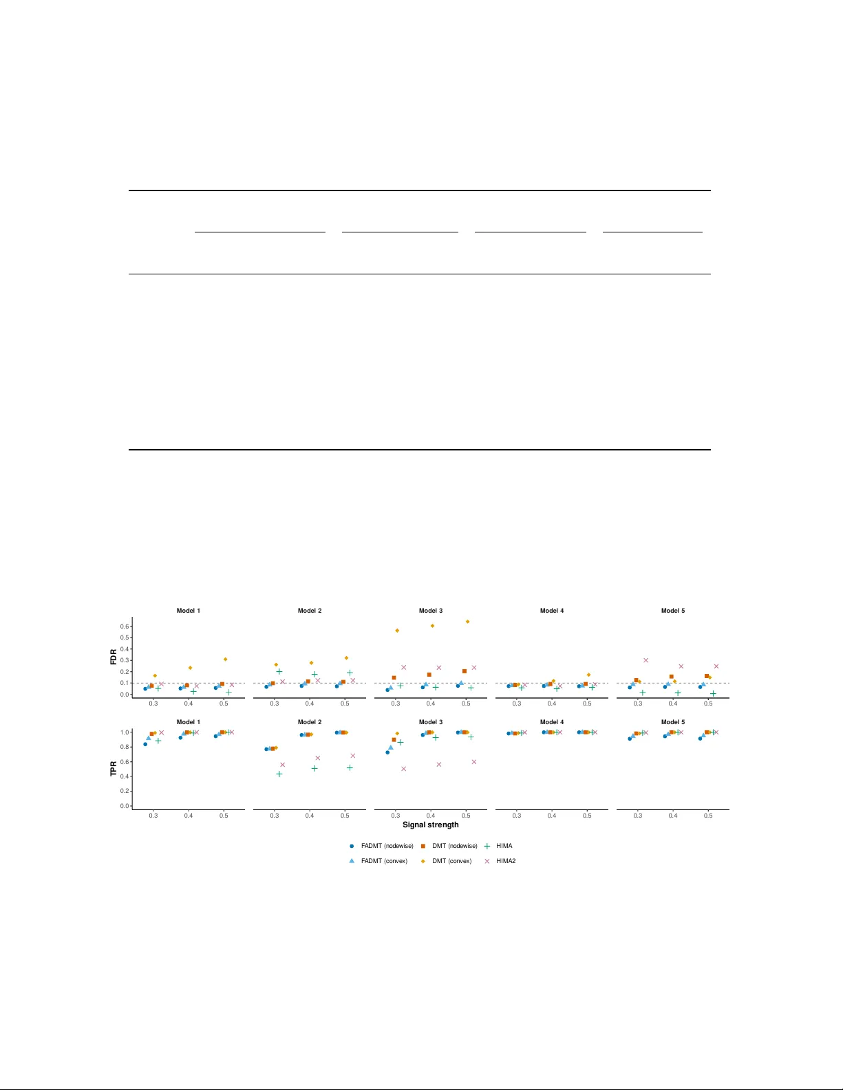
F actor-A djusted Multiple T esting for High-Dimensional Individual Mediation Eects Chen Shi 1 , Zhao Chen ∗ 1 , and Christina Dan W ang † 2 1 Sc ho ol of Data Science, F udan Universit y 2 Business Division, New Y ork Universit y Shanghai F ebruary 19, 2026 Abstract Iden tifying individual mediators is a central goal of high-dimensional mediation analysis, y et p erv asiv e dependence among mediators can inv alidate standard debiased inference and lead to substan tial false discov ery rate (FDR) ination. W e propose a F actor-A djusted Debiased Mediation T esting (F ADMT) framework that enables large-scale inference for individual mediation eects with FDR control under com- plex dep endence structures. Our approach p osits an appro ximate factor structure on the unobserv ed errors of the mediator mo del, extracts common latent factors, and con- structs decorrelated pseudo-mediators for the subsequen t inferential pro cedure. W e establish the asymptotic normality of the debiased estimator and develop a m ultiple testing pro cedure with theoretical FDR control under mild high-dimensional condi- tions. By adjusting for latent factor induced dep endence, F ADMT also improv es robustness to spurious associations driv en b y shared latent v ariation in observ ational studies. Extensiv e simulations demonstrate the sup erior nite-sample p erformance across a wide range of correlation structures. Applications to TCGA-BRCA m ulti- omics data and to China’s sto c k connect study further illustrate the practical utility of the prop osed metho d. K eywor ds: High-dimensional mediation analysis; High dimensional inference; F actor model; F alse discov ery rate ∗ Corresp onding author: zchen_fdu@fudan.edu.cn. † Corresp onding author: christina.w ang@nyu.edu. 1 1 In tro duction Understanding the mechanisms through which an exp osure aects an outcome is a central problem across man y scientic disciplines. Mediation analysis provides a principled frame- w ork for decomp osing the total eect into a direct eect and an indirect eect transmitted through intermediate v ariables ( Baron & Kenn y 1986 , MacKinnon et al. 2004 ). In mo dern genomics and m ulti-omics studies and increasingly in nance, hundreds or thousands of candidate mediators are routinely measured, making individual mediator disco v ery b oth scien tically imp ortan t and statistically c hallenging. T w o diculties are particularly acute in high dimensions: mediators exhibit strong dep endence driven b y shared latent v ariation, and iden tifying activ e mediators necessitates rigorous simultaneous inference to maintain false discov ery rate (FDR) control. A gro wing literature studies high-dimensional mediation, with m uc h of it fo cusing on inference for the ov erall indirect eect, whic h aggregates contributions from all mediators ( Huang & Pan 2016 , Zhou et al. 2020 , Guo et al. 2022 , 2023 , Lin et al. 2023 ). Although informativ e, ov erall indirect eects can mask imp ortan t mechanistic signals when individ- ual mediation eects cancel out due to opp osing directions. This motiv ates metho ds for individual mediation eect discov ery . Existing metho ds for testing individual mediation eects in high dimensions generally follo w t w o paradigms: marginal mo deling, whic h relies on simplifying indep endence as- sumptions and apply multiple testing to marginal regression co ecien ts ( Dai et al. 2022 , Liu et al. 2022 , Du et al. 2023 ) and joint mo deling, whic h emplo ys high-dimensional infer- ence or v ariable selection tec hniques suc h as screening, debiased Lasso, and adaptive Lasso ( Zhang et al. 2016 , 2021 , Derkach et al. 2019 , Shuai et al. 2023 ). While these approaches oer mo deling exibility , their v alidity is severely compromised by p erv asive dep endence among mediators. 2 Strong dep endence among mediators presen ts t w o fundamen tal c hallenges. First, high- dimensional inference or v ariable selection pro cedure rely on structural conditions suc h as irrepresen table condition for v ariable selection, or the compatibility/restricted eigen v alue (RE) conditions for v alid inference. Strong correlation can disrupt these regular conditions, leading to pro cedure failure ( F an et al. 2020 ). Second, controlling the FDR in large-scale m ultiple testing b ecomes dicult when test statistics are strongly dep enden t, violating the assumptions underlying many classical FDR pro cedures ( Benjamini & Ho c hberg 1995 , Benjamini & Y ekutieli 2001 , Storey et al. 2004 ). Empirical evidence sho ws that ignoring suc h dep endence can result in sev ere FDR ination ( W u 2008 , Blanc hard & Ro quain 2009 , F an, Han & Gu 2012 , F an et al. 2019 ). T o address these c hallenges, we propose a F actor-Adjusted Debiased Mediation T esting (F ADMT) framew ork for high-dimensional individual mediation analysis with FDR control. Our motiv ation is that dep endence among mediators in mo dern omics studies is often driven b y a few common factors, so that an appro ximate factor structure can provide a useful and parsimonious represen tation ( Bai 2003 , F an et al. 2013 ). By separating p erv asiv e factor- driv en dep endence from idiosyncratic v ariation, factor-adjusted metho ds ha ve been shown to substantially impro v e inference and multiple testing accuracy ( F an et al. 2019 , 2024 ). A fundamental dierence b et ween our setting and existing factor-adjusted framew orks is that traditional appro ximate factor mo dels are applied to observ able data, whereas w e inno v ativ ely apply factor analysis to the unobserved errors of the mediator mo del. This requires a tw o-step construction: we rst estimate the latent factor comp onen t and obtain estimated idiosyncratic comp onen ts, which serve as decorrelated pseudo-mediators. W e then use these pseudo-mediators for downstream debiased inference and multiple testing. This shift introduces new tec hnical c hallenges as the rst-step estimation error propagates in to do wnstream pro cedure. W e establish the asymptotic normality of the debiased estimator under mild regular con- 3 ditions and develop a theoretically v alid FDR control rule for individual mediation eects. Extensiv e sim ulations further demonstrate strong nite-sample p erformance: F ADMT con- trols FDR across a wide range of dep endence structures while maintaining comp etitive p o wer relativ e to existing metho ds. W e further apply our metho d to a multi-omics dataset from the TCGA-BR CA cohort, inv estigating whether DNA methylation mediates the ef- fect of age at diagnosis on MKI67 gene expression, and to a nancial sto c k connect setting, examining whether mark et liberalization aects rms’ idiosyncratic risk through c hanges in corp orate fundamen tals. These applications demonstrate the metho d’s abilit y to uncov er in terpretable mediation eects in real-world high-dimensional data across domains. This pap er makes sev eral k ey con tributions. First, in the theory of high-dimensional inference and FDR con trol under strong dep endence, w e provide a rigorous foundation for large-scale m ultiple testing in settings where classical FDR pro cedures can fail due to p erv asiv e correlations. Rather than relying on indep endence or weak-dependence assump- tions, w e establish a factor-adjusted framew ork whic h enables accurate FDR con trol even in strongly correlated, high-dimensional regimes. This oers a general theoretical resolution to a long-standing challenge in high-dimensional inference. Second, at the metho dological lev el of factor-adjusted inference, w e expand the existing paradigm by mo ving factor adjustment from observ able quan tities to a latent error structure. Unlik e F ARM ( F an et al. 2024 ) and F armT est ( F an et al. 2019 ), whic h impose factor mo dels on observ ed v ariables, our framework p osits and exploits an appro ximate factor structure in the unobserved errors of the mediator mo del. Third, w e instantiate these theoretical and metho dological dev elopmen ts in high- dimensional individual mediation testing under a comp osite n ull. F or the pro duct-form mediation eect, w e prop ose and analyze a MaxP-based, factor-adjusted testing pro cedure that explicitly accoun ts for the union structure of the null hypothesis. Moreo v er, our framew ork impro v es robustness to latent common-factor dep endence that manifests as 4 p erv asiv e shared comp onen ts driving strong correlations among mediators. By estimating and adjusting for these latent factors through the mediator error structure, F ADMT separates shared v ariation from mediator-sp ecic signals, stabilizes downstream inference, and enhances the interpretabilit y of disco v ered mediation ndings. W e adopt the following notations throughout the article. F or a v ector , w e denote its and norms b y and , resp ectiv ely . The sub- Gaussian norm of a random v ariable is dened as inf exp , and for a random vector , sup . F or a matrix , w e let max max , b e its F robenius norm, and (or ) b e its and sp ectral norms. min and max denote the minimum and maxim um eigen v alues of a square matrix . F or any set , denotes its cardinality , and . F or t w o p ositiv e sequences and , w e write if there exists a p ositiv e constant such that for all sucien tly large , and if as . Similarly , and indicate that the corresp onding relationships hold in probability . The rest of the article is organized as follows. Section 2 introduces the mo del and h y- p otheses and presen ts the prop osed factor-adjusted debiased inference and multiple testing pro cedure. Section 3 establishes theoretical guarantees, including asymptotic v alidit y and FDR control. Section 4 rep orts simulation studies. Section 5 presen ts data applications, and Section 6 concludes the pap er. 2 Metho dology 2.1 Problem Setup W e consider a high-dimensional mediation framework with indep enden t and iden tically distributed (i.i.d.) observ ations m , where is the outcome, is the 5 exp osure (or treatmen t), and collects candidate mediators. W e allow the n um b er of mediators to exceed the sample size , accommo dating high- dimensional settings. The underlying relationships among these v ariables are mo deled via the following linear structural equations: (1) (2) where captures the mediator-outcome eects, and captures the exp osure-mediator eects. The errors are i.i.d. with and Var . The residual vectors are i.i.d. with 0 and Cov . W e assume is indep enden t of and is indep enden t of . In matrix form, let denote the outcome vector, the exp osure vector, and the mediator design matrix. W e also write and . Substituting ( 2 ) into ( 1 ) yields the reduced-form mo del for the outcome: (3) In this expression, captures the direct eect of the exp osure on the outcome , and is the total (aggregate) mediation eect through all mediators. Prior work has primarily fo cused on testing the o v erall mediation eect ( Zhou et al. 2020 , Guo et al. 2023 , Lin et al. 2023 ): H H While testing the ov erall mediation eect pro vides a global assessment of whether medi- ators collectiv ely transmit the eect of the exp osure on the outcome, it do es not rev eal whic h sp ecic mediators are resp onsible for the observ ed indirect eect. This limitation is 6 esp ecially p ertinent in high-dimensional settings, where the eects of individual mediators ma y v ary in direction, p oten tially canceling eac h other out in the ov erall eect. There- fore, testing individual mediation eects b ecomes essen tial for identifying sp ecic activ e mediators and understanding the underlying causal mechanisms in greater detail. Our goal is to test individual mediation eects for eac h mediator , dened as the pro duct . The corresp onding h yp otheses are stated as: H H T esting these individual h yp otheses in high-dimensional settings presen ts several challenges. First, the regime where necessitates regularized estimation. Classical estimators tend to b e biased in high dimensions due to regularization eects, which calls for debi- ased estimation metho ds. Second, mediators often exhibit complex dep endencies due to shared biological path w a ys or laten t factors. These dep endencies p ose signicant challenges for b oth v ariable selection and statistical inference. Third, the simultaneous testing of h yp otheses requires rigorous control of the F alse Discov ery Rate (FDR). Standard FDR pro cedures ma y suer from inated error rates under the strong dep endence, emphasizing the imp ortance of dep endence-adjusted m ultiple testing frameworks. 2.2 Laten t F actor A djustmen t and Mo del Reformulation T o mitigate the strong dep endence among mediators, w e adopt a factor-adjusted strategy inspired b y recent work on high-dimensional inference under latent factor structures ( F an et al. 2019 , 2024 ). The k ey idea is to remov e a lo w-rank common comp onen t that drives most cross-mediator correlations, and to use the estimated idiosyncratic comp onen ts for do wnstream inference. W e work with the mediator-equation errors in ( 2 ), whic h capture the v ariation in 7 not explained by the exposure . W e assume an appro ximate factor mo del: where are laten t factors, is the loading matrix, and are idiosyn- cratic comp onen ts with weak dep endence. A crucial distinction b et ween our framew ork and traditional factor analysis where mo dels are typically applied to observ able data is that is unobserv ed. Consequently , we must rst estimate it b y using the OLS estimator . This additional estimation step introduces a rst-stage error, whic h propagates into the subsequen t factor extraction and high-dimensional inference. Let , and . W e apply prin- cipal comp onen t analysis ( Bai 2003 , F an et al. 2013 ) to the estimated residual matrix to obtain the latent factors and loadings. Under standard iden tiabilit y conditions: Cov and is diagonal The estimators are derived as follows: the columns of F are the eigenv ectors of corresp onding to the top eigen v alues, B F , and . Remark 1. A pr actic al c onsider ation is the choic e of the numb er of factors . Ther e have b e en various metho d to estimate the numb er of factors ( Bai & Ng 2002 , L am & Y ao 2012 , A hn & Hor enstein 2013 , F an et al. 2022 ).W e adopt the eigenvalue r atio metho d in L am & Y ao ( 2012 ), Ahn & Hor enstein ( 2013 ), which is widely use d in the factor mo deling liter atur e and yields a c onsistent estimator for the numb er of factors . L et b e the -th lar gest eigenvalue of and max b e a pr escrib e d upp er b ound. Then, the numb er of factors is given by arg max max 8 With the factor structure iden tied, w e can decomp ose the mediator matrix as . Substituting this decomp osition into the outcome mo del ( 1 ) and rear- ranging terms, we arriv e at the factor-adjusted regression framework: (4) where and are treated as n uisance parameters. This re- form ulation allo ws us to explicitly adjust for shared laten t dependencies among mediators, while leveraging the decorrelated idiosyncratic residuals as pseudo-predictors for infer- ence. This transformation enables v alid inference even in the presence of strong dependence and high dimensionalit y , as will b e demonstrated in our theoretical and numerical analyses. 2.3 T est Statistic Building on the factor-adjusted mo del, we now develop the inferential pro cedure for indi- vidual mediation eects. A widely adopted strategy in mediation literature is the joint signicance test (also known as the MaxP test) in MacKinnon et al. ( 2002 ), which has b een shown to outp erform the Sob el test in b oth theoretical and empirical studies ( Liu et al. 2022 , Du et al. 2023 ). The MaxP test rejects the null h yp othesis only when b oth comp onen ts are statistically signicant. Sp ecically , let and b e the -v alues for testing and , resp ectiv ely . The test statistic is dened as: max max While can b e readily obtained via standard OLS regression, constructing a v alid -v alue for in ( 4 ) is challenging due to the high-dimensionality and the laten t dep endence structure. T o this end, w e emplo y a factor-adjusted debiased Lasso approach to reco v er asymptotic normality for the estimated mediator-outcome eects. 9 Recalling the augmented Equation ( 4 ), we obtain an initial p enalized estimator of b y tting a high-dimensional regression of on , treating the coecients on as nuisance parameters. Sp ecically , we solv e arg min (5) Due to regularization, is biased. F ollowing the debiasing framework for high- dimensional M-estimators ( Ja v anmard & Mon tanari 2014 , V an de Geer et al. 2014 ), we dene the debiased estimator as: where serv es as a decorrelating matrix. Using the orthogonality prop erties and , the error of the debiased estimator can b e decomp osed as: where . The rst term represents the leading sto c hastic comp onen t with asymptotic v ariance , while the second term is the bias that b ecomes negligible under appropriate regular conditions. The decorrelating matrix can b e constructed via no de-wise Lasso regression ( V an de Geer et al. 2014 , Jav anmard & Montanari 2018 ) or constrained conv ex optimization ( Ja v anmard & Montanari 2014 , Battey et al. 2018 ). W e pro vide details for these approaches in the App endix and compare their nite-sample p erformance in Section 4. Remark 2 (Orthogonalit y of the pseudo-mediators) . By c onstruction, the estimate d id- iosyncr atic c omp onent matrix satises 0 and 0 . Sinc e is the OLS r esidual matrix fr om r e gr essing on , we have . Given that is derive d fr om the princip al c omp onents of , its c olumns lie in the c olumn sp ac e of , implying . Conse quently, also satises . 10 Based on the asymptotic normality of the debiased estimator established in Theo- rem 1 , the -v alue for testing is given by: where denotes the cumulativ e distribution function (CDF) of the standard normal distribution, is a consistent estimator for . By combining with the -v alue obtained from the rst-stage OLS regression, w e arrive at the joint signicance test statistic max max for eac h . The complete pro cedure is summarized in Algorithm 1 . 2.4 Multiple T esting and FDR Control W e aim to sim ultaneously test the mediation hypotheses v ersus for . Let max max b e the MaxP -v alue. F or a threshold , dene the rejection set max with . Let b e the set of true mediation nulls and b e the n um b er of false discov eries. F alse Discov ery Prop ortion (FDP) and FDR are dened as: FDP FDR FDP A unique c hallenge in mediation analysis is that the n ull h ypothesis H is a composite n ull, represen table as the union of three disjoint cases: H H H W rite for their prop ortions among all tests. Standard FDR pro cedures, suc h as the Benjamini-Ho c hberg (BH) metho d, assume a uniform distribution for 11 Algorithm 1 F actor-adjusted debiased inference for individual mediation eects Require: Data with . Ensure: MaxP -v alues max for . 1: Path A (exp osure mediator). F or each , regress on b y OLS to obtain and the -v alue . Let . 2: Residual factor extraction. Apply PCA to to obtain and the estimated idiosyncratic comp onen t matrix . 3: F actor-adjusted Lasso. Fit the p enalized regression of on with an p enalt y on (as in ( 5 )), yielding . 4: Debiasing. Construct a decorrelating matrix (no dewise Lasso or conv ex optimiza- tion). F orm the debiased estimator 5: Path B (mediator outcome) -v alues. Compute and a consistent . F or each , compute 6: MaxP combination. Output max max for . n ull -v alues ( Benjamini & Ho c h b erg 1995 , Benjamini & Y ekutieli 2001 ). How ever, under the double-n ull H , follo ws Beta(2,1) distribution, as sho wn in Liu et al. ( 2022 ), Dai et al. ( 2022 ). This deviates from the standard uniform reference and mak es BH-type pro cedures o v erly conserv ativ e. Motiv ated b y recen t dev elopmen ts in mediation testing, w e construct a mixture null distribution to estimate the FDP more accurately ( Liu et al. 2022 , Dai et al. 2022 ). Under the high-dimensional sparse mo deling framework, we assume that most mediators ha v e no eect on the outcome. Consequently , the prop ortion of null cases where only the 12 mediator-outcome eect is presen t ( ) is negligible, and we fo cus on the mixture of H and H . W e estimate the prop ortion of n ull exp osure-mediator eects, , using Storey’s metho d ( Storey 2002 ): 1 (6) where is a tuning parameter. This estimator assumes that most large v alues come from true null hypotheses and are uniformly distributed. F or well-c hosen , ab out of the v alues lie in the interv al . Therefore, the prop ortion of v alues that exceed should b e close to . Under sparsity , serves as an estimate for , while estimates . Remark 3. A value of is use d in the SAM softwar e in Stor ey ( 2003 ). Blanchar d & R o quain ( 2009 ) suggests to use e qual to the signic anc e level for dep endent values. W e fol low Stor ey et al. ( 2004 ) to adopt a b o otstr ap-b ase d automatic sele ction for . Using the estimated null proportions, w e dene the adjusted FDP estimator as: FDP 1 (7) F or a target FDR level , the optimal signicance threshold is determined b y: sup FDP (8) Theoretical results sho w this pro cedure controls the FDR asymptotically under appropriate regularit y conditions. The full pro cedure is detailed in Algorithm 2 . 3 Theoretical Results This section establishes the theoretical foundations of the prop osed factor-adjusted infer- ence framework. W e b egin by outlining the regularit y conditions, then derive the con- v ergence rates for the estimated latent structures. Finally , we establish the asymptotic normalit y of the debiased estimator and the v alidity of the FDR con trol pro cedure. 13 Algorithm 2 FDR control for MaxP -v alues Require: ; target level ; tuning . 1: Compute max max for all . 2: Estimate b y ( 6 ) (with selected as in Storey et al. 2004 ). 3: F or in the set of observed max , compute FDP in ( 7 ). 4: Set b y ( 8 ) and reject max . 3.1 Regularit y Conditions and Error Propagation T o accommo date the high-dimensional setting, w e imp ose the follo wing assumptions on the data-generating pro cess and the latent factor structure. Assumption 1 (Sub-Gaussianit y) . The se quenc e ar e i.i.d. r andom ve ctors. The exp osur e is sub-Gaussian with . The latent factors and idiosyncr atic c omp onents ar e zer o me an sub-Gaussian ve ctors such that and for some p ositive c onstant . Assumption 2 (Perv asiv e Condition) . A l l the eigenvalues of B B ar e b ounde d away fr om 0 and as . That is, min B B max B B . Assumption 3 (Loading matrix and Idiosyncratic comp onen t) . L et Cov . A s- sume min , , min var for some c onstants , and max for some c onstant . In addition, for al l ther e exists such that and . Remark 4. A ssumption 1 is standar d for high-dimensional infer enc e, ensuring that tail b ehaviors ar e wel l-c ontr ol le d via c onc entr ation ine qualities. A ssumptions 2 and 3 is c ommon in factor mo dels ( F an et al. 2013 , 2020 , 2024 ). T o gether, A ssumptions 2 and 3 ensur e that and c an b e c onsistently estimate d by the PCA metho d . A distinctive feature of our framework is that the factor mo del is tted to estimated 14 residuals. The following prop osition quan ties the error in tro duced by the rst-stage OLS estimation. Prop osition 1. Under A ssumption 1, we have max log log Prop osition 1 sho ws the OLS estimation error which propagates in to the factor extrac- tion pro cess. This rate determines the precision of the estimated idiosyncratic comp onen t , which serve as our pseudo-predictors. W e dene log log for notational con v enience. Prop osition 2. Supp ose A ssumptions 1-3 hold. L et , wher e is a diagonal matrix c ontaining the rst lar gest eigenvalues of . Then: 1. max 2. 3. max log Remark 5. The r esults extend classic al PCA err or b ounds (e.g., F an et al. 2013 ) to the pr esent two-stage setting, wher e PCA is applie d to r ather than the unobserve d . The additional term quanties the imp act of the rst-stage r esidual-pr oxy err or. 3.2 Asymptotic Normalit y of the Debiased Estimator T o establish the v alidity of the individual mediation tests, we require the debiased esti- mator to b e asymptotically normal. In the theory b elo w, w e fo cus on constructing the decorrelating matrix via no dewise Lasso. This necessitates a sparsity condition on the mediator-outcome eects and the precision matrix of the idiosyncratic errors. Accordingly , the following sparsity conditions are imp osed on the precision matrix , which are standard for no dewise-Lasso-based debiasing. 15 Assumption 4 (Sparsity) . L et and let wher e . L et denote the dimension of the unp enalize d nuisanc e p ar ameter . A ssume log log max log log Assumption 5 (Consistent Estimation of ) . A ssume . Remark 6. A ssumption 4 imp oses a sp arsity c ondition to ensur e the asymptotic normality of the debiase d L asso estimator. Pr evious studies have establishe d that log is the sp arisity c ondition for c onsistent estimation ( Candes & T ao 2007 , Bickel et al. 2009 ), while log is the c ondition for asymp otic normality ( V an de Ge er et al. 2014 , Javanmar d & Montanari 2014 , Zhang & Zhang 2014 ). W e adopt a similar sp arsity c ondition up to the lo garithmic factor to ac c ount for the additional c omplexity intr o duc e d by the factor estimation. The sp arsity assumption for is standar d in high-dimensional infer enc e using no dewise L asso ( V an de Ge er et al. 2014 , Javanmar d & Montanari 2018 ). Under the usual sub-Gaussian assumption, the sp arsity r e quir ement on is typic al ly max log . W e also adopt a similar sp arsity c ondition, with an additional log factor in the denominator, to ac c ount for the extr a c omplexity intr o duc e d by the factor estimation step. A ssumption 5 holds when is c ompute d by r ette d cr oss-validation in F an, Guo & Hao ( 2012 ) or sc ale d lasso in Sun & Zhang ( 2013 ). Theorem 1. Under A ssumptions 1-4, and assuming that the err or term .L et log in the factor-adjuste d L asso ( 5 ), and let the no dewise-L asso tuning p ar ameters satisfy the same or der uniformly in . Then 0 wher e . 16 Corollary 1. Under the c onditions of The or em 1 , for any , the debiase d -value is asymptotic al ly uniform c onditional on . Sp e cic al ly, for any , sup Pr as Conse quently, for any -me asur able statistic , is asymptotic al ly indep endent of . Remark 7. In nite samples, the debiase d infer enc e for may exhibit mild c onserva- tiveness, manifesting as -values that ar e sto chastic al ly lar ger than the uniform distribution (i.e., sup er-uniform) under the nul l hyp othesis. This b ehavior is primarily attribute d to factor-estimation err or and the r e gularization involve d in c onstructing . Such c onserva- tiveness do es not c ompr omise the validity of the FDR c ontr ol pr o c e dur e. Sinc e the FDR c ontr ol fr amework r elies on the FDP estimator b eing a c onservative upp er b ound, sup er- uniform nul l -values mer ely r esult in a mor e pr ote ctive thr eshold. 3.3 V alidit y of FDR Con trol Finally , we sho w that the prop osed FDR con trol pro cedure is v alid. W e mak e the following assumptions for our asymptotic results. Assumption 6 (Empirical conv ergence of and sparsit y) . L et denote the four c omp onent sets, and for as . (i) (Empiric al tail c onver genc e of ) F or , ther e exist c ontinuous functions such that for al l , 1 almost sur ely Mor e over, for (i.e., ), ar e asymptotic al ly Unif and satisfy the c orr esp onding empiric al c onver genc e. (ii) (Sp arsity) . 17 Remark 8. A ssumption 6 r e quir es the almost sur e p ointwise c onver genc e of the empiric al -value pr o c esses, a c ondition widely use d in establishing FDR c ontr ol ( Stor ey et al. 2004 , Dai et al. 2022 ). A ssumption 6 do es not pr e clude str ong cr oss-se ctional c orr elation in which is explicitly mo dele d thr ough a low-dimensional latent factor structur e. In p articular, str ong dep endenc e induc e d by a xe d numb er of p ervasive factors is c omp atible with empir- ic al c onver genc e, pr ovide d that the r emaining idiosyncr atic c omp onents exhibit only we ak dep endenc e. Theorem 2. A ssume The or em 1 and Cor ol lary 1 hold, and A ssumption 6 holds. A s , FDP is a c onservative estimate of FDR for al l that satises . Mor e over, the signic anc e thr eshold expr esse d in ( 8 ) c ontr ols the FDR at level : FDP and lim sup FDR Remark 9. The c onservativeness of FDP is establishe d p ointwise over an admissible set of ’s, r ather than uniformly for al l . This phenomenon is standar d for mixtur e- b ase d FDP estimators under c omp osite (union) nul ls; se e Dai et al. ( 2022 ) for an analo gous c ondition. Inde e d, is typic al ly chosen close to , and the distribution of -values under alternative hyp othesis is sto chastic al ly less than the uniform distribution. The c ondition should hold for the smal l signic anc e cutos typic al ly use d in multiple testing. 4 Sim ulation Studies In this section, w e conduct Monte Carlo simulations to inv estigate the nite-sample p erfor- mance of our prop osed F actor-A djusted Debiased Mediation T esting (F ADMT) and com- pare it with existing metho dologies. W e consider a sample size and mediators. The exp osure is generated as . The mediators are generated as , where . W e 18 set the exp osure-mediator eects for , and for . The resp onse is generated from , where , , and the mediation-outcome eects are . The parameter represents the signal strength. The sim ulation results are based on 200 replications. The target FDR lev el is set to . W e consider ve co v ariance structures for corresp onding to Mo del 1 through Mo del 5: Mo del 1 (AR): Assume the cov ariance matrix b eing an AR correlation structure. That is . Mo del 2 (F actor Mo del): Assume are generated from three factor mo del B , where factors , the element of loading matrix B is generated from a uniform distribution , and . Mo del 3 (Comp ound Symmetric): Consider a symmetric matrix with diagonal ele- men ts 1 and each o-diagonal elemen t equals 0.8. Mo del 4 (Long Memory): Consider where each elemen t is defıned as , with Mo del 4 is from Bick el & Levina ( 2008 ) and has also recen tly b een considered by F an & Han ( 2017 ) for strong long memory dep endence. Mo del 5 (Indep enden t): . W e compare the proposed F ADMT (F actor-A djusted Debiased Mediation T esting) with an ablation baseline DMT (Debiased Mediation T esting), whic h applies the same debiased inference and the same multiple-testing pip eline but without factor adjustment. F or each of F ADMT and DMT, we consider t w o constructions of the decorrelating matrix : (i) no dewise regression ( V an de Geer et al. 2014 ) and (ii) conv ex optimization ( Jav anmard & Mon tanari 2014 ). In addition, we include tw o metho ds for high-dimensional individual mediation eect testing under sparse linear mo dels, HIMA ( Zhang et al. 2016 ) and HIMA2 19 ( P erera et al. 2022 ) 1 . Let b e the selected set of mediators at FDR lev el . W e report the empirical a v erage false discov ery prop ortion (FDP) and true p ositiv e rate (TPR), where TPR is obtained by a v eraging the prop ortion of correctly selected mediators o v er 200 rep etitions. T able 1 rep orts the o v erall FDR and TPR for F ADMT and DMT under signal . A cross all cov ariance designs, F ADMT con trols FDR at the nominal level , while DMT can exhibit substantial ination, esp ecially under strong dep endence. This isolates the practical b enet of factor adjustment in stabilizing debiased inference for . T able 1 further rev eals dierence b et ween the t w o constructions of the decorrelating matrix, namely no dewise Lasso regression and conv ex optimization. F or the DMT metho d, the conv ex optimization approach generally leads to worse FDR con trol than no dewise Lasso across most dep enden t designs, likely reecting the dicult y of solving the opti- mization problem accurately when the mediator cov ariance structure is highly correlated. Only in Mo del 5, where mediators are indep enden t, do es conv ex optimization outp erform no dewise Lasso in terms of FDR control. Interestingly , this pattern reverses under the prop osed F ADMT framework. Both no dewise Lasso and conv ex optimization ac hieve v alid FDR control after factor adjustment, but no dewise Lasso tends to b e more conserv ative, often yielding t yp e I error rates for inference on b elo w the nominal level and cor- resp ondingly conserv ative FDR v alues. In contrast, con v ex optimization attains higher p o wer while maintaining accurate FDR con trol. This improv ement can b e attributed to the factor adjustmen t step, whic h eectively remo v es cross-sectional dep endence among mediators and simplies the residual cov ariance structure. As a result, con v ex optimiza- tion b ecomes more ecient and b enets from its v ariance-minimization ob jectiv e, leading to reduced estimator v ariance and enhanced p ow er. F rom a practical p erspective, these gains are particularly app ealing, as conv ex optimization is computationally substantially 1 Both HIMA and HIMA2 are implemen ted using the HIMA R package, with their default metho ds. 20 more ecient than no dewise Lasso. Consequen tly , the prop osed F ADMT metho d not only impro v es statistical stability under dependence but also amplies the computational adv an- tages of conv ex optimization in large-scale applications. A dditional decomp osition results, including the Type I error and p o w er for testing individual and eects, are re- p orted in Appendix B.1 . W e also assess the con v ergence of the empirical -v alue pro cesses in the App endix B.2 , showing that the empirical distributions of the null and max closely follow their theoretical references. These results provide empirical supp ort for the theoretical guarantees established in Theorem 2 . T o further inv estigate the robustness of F ADMT, we v ary the signal strength , aecting both and sim ultaneously . Figure 1 compares F ADMT with DMT, HIMA, and HIMA2 across all ve co v ariance designs and signal lev els. As sho wn in Figure 1 , F ADMT consisten tly con trols the FDR at the nominal lev el across all signal strengths and all cov ariance mo dels, for both the no dewise Lasso and con v ex optimization implemen tations. In con trast, competing metho ds exhibit pronounced FDR ination in the presence of strong dep endence among mediators. In particular, under Mo dels 2 and 3, DMT, HIMA, and HIMA2 frequen tly exceed the target FDR lev el. Mean while, the impro v ed FDR con trol of F ADMT do es not come at the exp ense of statistical p o wer. A cross all signal lev els, the TPR ac hieved by F ADMT is comparable to that of existing methods.This results highligh t the robustness of F ADMT in simultaneously main taining v alid error control and comp etitiv e p o w er in challenging high-dimensional settings. 21 T able 1: Overall FDR and TPR under ve mo dels with . F ADMT (nodewise) F ADMT (con v ex) DMT (no dewise) DMT (conv ex) Mo del FDR TPR FDR TPR FDR TPR FDR TPR 1 0.0568 0.9470 0.0725 0.9710 0.0918 1.0000 0.3098 1.0000 2 0.0708 0.9955 0.0948 0.9955 0.1109 0.9955 0.3209 0.9960 3 0.0750 0.9965 0.0973 1.0000 0.2043 1.0000 0.6420 1.0000 4 0.0713 1.0000 0.0750 1.0000 0.0919 1.0000 0.1727 1.0000 5 0.0647 0.9145 0.0848 0.9520 0.1623 1.0000 0.1497 1.0000 Mo d e l 1 Mo d e l 2 Mo d e l 3 Mo d e l 4 Mo d e l 5 0 . 3 0 . 4 0 . 5 0 . 3 0 . 4 0 . 5 0 . 3 0 . 4 0 . 5 0 . 3 0 . 4 0 . 5 0 . 3 0 . 4 0 . 5 0 . 0 0 . 1 0 . 2 0 . 3 0 . 4 0 . 5 0 . 6 F D R Mo d e l 1 Mo d e l 2 Mo d e l 3 Mo d e l 4 Mo d e l 5 0 . 3 0 . 4 0 . 5 0 . 3 0 . 4 0 . 5 0 . 3 0 . 4 0 . 5 0 . 3 0 . 4 0 . 5 0 . 3 0 . 4 0 . 5 0 . 0 0 . 2 0 . 4 0 . 6 0 . 8 1 . 0 Si g n a l s tr e n g th T PR F A D MT ( n o d e w i s e ) F A D MT ( c o n v e x ) D MT ( n o d e w i s e ) D MT ( c o n v e x ) H I MA H I MA 2 Figure 1: Comparison of FDR and TPR across dierent metho ds and signal strengths. 22 5 Data Application 5.1 Biomedical Application T o demonstrate the practical utility of our prop osed metho dology , we apply it to multi- omics data from the TCGA-BRCA cohort 2 , fo cusing on the role of DNA methylation in mediating the relationship b et ween age at diagnosis and the expression of MKI67, a w ell- established proliferation marker in breast cancer. Previous studies hav e shown that aging is accompanied by systematic c hanges in gene expression and epigenetic mo dications that can inuence cancer developmen t and progression ( Baylin & Jones 2011 , Raky an et al. 2011 ). In particular, DNA methylation alterations ha v e b een rep orted to mediate transcriptional regulation in an age-dep enden t manner ( Chatsirisupachai et al. 2021 ). Data were retriev ed from the GDC p ortal via the R package TCGAbiolinks , including RNA-seq, DNA methylation (Illumina HumanMethylation450K), and clinical records. Af- ter prepro cessing, we retained 811 samples with complete data for age, meth ylation, gene expression, and co v ariates (race and AJCC pathologic stage). The RNA-seq coun ts for MKI67 w ere normalized using DESeq2’s v ariance-stabilizing transformation (vst) to ad- dress heteroscedasticity , while DNA meth ylation -v alues were con v erted to M-v alues via logit transformation ( log ) as recommended b y Du et al. ( 2010 ) to impro ve normalit y . Age at diagnosis (range: 26-89 years; mean ± SD: 58.0 ± 13.3) served as the exp osure v ariable, and 299,813 CpG sites with non-missing v alues across all samples were included as p oten tial mediators. The transformed MKI67 expression lev els constituted the outcome v ariable, adjusted for race and tumor stage. F ollowing Guo et al. ( 2022 ) we rst carry out a screening step to retain the top 1000 p oten tial mediators by ranking the absolute v alue of the pro duct of tw o correlations—the correlation b etw een exp osure v ariable and eac h element of mediators, and betw een outcome 2 Data a v ailable at https://portal.gdc.cancer.gov/projects/TCGA- BRCA. 23 and eac h elemen t of mediators. This indeed is a marginal screening pro cedure based on P earson correlation prop osed b y F an & Lv ( 2008 ). They sho w that for linear mo dels, under some regularity conditions, the screening pro cedure p ossesses a sure screening property . W e then emplo y our proposed F actor-A djusted Debiased Mediation T esting (F ADMT) metho d to statistically test the mediation eects of individual CpG sites. Under a presp ecied false disco v ery rate (FDR) lev el of 0.1, w e iden tify DNA meth ylation sites with signicant mediation eects and further analyze their p oten tial biological mec hanisms. In T able 2 , we rep ort the summary results on the three selected mediators by our metho d. Three CpG sites were identied as signicant mediators of age-associated MKI67 expression (FDR-adjusted -v alue < 0.1). The strongest mediation signal is observ ed at an in tergenic site c h.2.71774667F (chr2:71921159), lo cated near LINC01807. This site shows negativ e age-to-methylation and meth ylation-to-expression eects, resulting in a p ositiv e total mediation eect ( ). Biologically , this nding suggests that age-related h yp ometh ylation at this lo cus migh t lead to the do wnregulation of LINC01807. Giv en that long non-co ding RNAs hav e b een implicated in the regulation of chromatin architecture and gene expression ( Li et al. 2016 ), the observed eect is consistent with the hypothesis that reduced LINC01807 expression may relieve repression on the MKI67 promoter, thereb y enhancing cellular proliferation. The CpG site cg10404601 (chr19:8468449), lo cated in the 3’ UTR of RAB11B, exhibits a negative age-to-methylation eect and a p ositiv e meth ylation-to-expression asso ciation, yielding a negative mediation eect ( ). This pattern suggests that age- asso ciated hypomethylation may reduce RAB11B expression, ultimately leading to sup- pressed MKI67 levels and decreased cell proliferation. Supp orting the biological relev ance of this lo cus, RAB11B-AS1, a natural an tisense transcript of RAB11B, has b een sho wn to promote angiogenesis and metastasis in breast cancer by enhancing the expression of angiogenic factors suc h as VEGF A and ANGPTL4 in a hypoxia-inducible manner ( Niu 24 et al. 2020 ). This evidence highlights the p oten tial regulatory imp ortance of the RAB11B region in breast cancer progression. Lastly , cg24461063 (chr12:124971775), lo cated in the gene b ody of NCOR2, shows a mo derate negative eect of age on methylation and a stronger p ositiv e eect of meth ylation on expression, resulting in a negative mediation eect ( ). This is consisten t with NCOR2’s kno wn function as an estrogen receptor (ER ) corepressor: h yp ometh ylation ma y lead to upregulation of NCOR2, whic h in turn inhibits ER signaling and attenuates proliferativ e activity ( T sai et al. 2022 ). Collectively , these ndings provide biologically plausible insigh ts into the epigenetic regulation of proliferation in breast cancer. The observ ed mediation eects are supp orted b y previous studies on cancer epigenomics in Ba ylin & Jones ( 2011 ), Rakyan et al. ( 2011 ) and highlight the complex in terpla y b et w een aging, DNA methylation, and gene expression. T able 2: Summary of selected CpGs with signicant mediation eects CpGs Chromosome Neighboring gene max adj-P c h.2.71774667F c hr2:71921159 LINC01807 -0.2006 -0.0130 8.53 0.0001 cg10404601 c hr19:8468449 RAB11B -0.4973 0.0074 1.26 0.0631 cg24461063 c hr12:124971775 NCOR2 -0.2070 0.0223 2.12 0.0705 Notes: max represen ts the unadjusted -v alue for the mediation eect; adj-P denotes FDR-adjusted -v alue. 5.2 Financial Application W e next provide a nancial case study to illustrate the applicability of our mediation eect testing framew ork in nancial scenarios. W e study whether the launch of the Shanghai– Hong Kong Sto c k Connect aects rms’ long-run idiosyncratic risk through c hanges in corp orate fundamentals. Sto c k Connect is widely viewed as a quasi-natural exp erimen t 25 of partial equit y market lib eralization in China. Existing studies do cumen t that this pro- gram can aect market quality , corp orate p olicies, and rm risk-related outcomes through through changes in inv estor base and information environmen t ( Ma et al. 2019 , Xu et al. 2020 , Xiong et al. 2021 , Li et al. 2024 ). How ever, existing mechanism analyses t ypically consider only a small n um b er of candidate c hannels. In contrast, we study the mecha- nism question in a high-dimensional mediation setting by jointly analyzing a broad set of corp orate accoun ting and v aluation indicators with strong dep endence. Our empirical design adopts a tw o-p erio d dierence-in-dierences framework around the p olicy date 2014/11/17, when the rst batch of 568 sto c ks b ecame eligible for north b ound trading. F or each sto c k , we measure the change in rm-sp ecic risk as , where and are computed from daily Capital Asset Pricing Mo del (CAPM) residuals in the pre window (2014/05/22–2014/11/14) and the p ost window (2014/11/17– 2015/05/14), eac h spanning 120 trading da ys (ab out six mon ths) 3 . The treatmen t indicator equals one if sto c k is included in Sto c k Connect at , and zero otherwise. T o mitigate selection on observ ables, we implemen t a prop ensit y score matching (PSM) design with 1:1 matching without replacement, using a calip er of times the standard deviation of the propensity score ( Rosen baum & Rubin 1985 , Austin 2011 ). Poten tial con- trols are Shanghai-listed sto c ks that were not included in Sto c k Connect during the p ost windo w 4 . W e match on industry , market capitalization, b ook-to-market (all measured at 2014Q3), and pre-window idiosyncratic volatilit y . F rom 403 p oten tial con trols, the pro ce- dure yields 129 v alid matched pairs (258 observ ations) after removing 13 pairs with fewer than 50 trading-da y observ ations in the p ost windo w. Daily returns, industry classications, 3 W e remo ve the common mark et comp onen t by estimating the CAPM model and then dening as the standard deviation of the tted residuals within the corresp onding windo w. This construction isolates rm-specic uctuations after controlling for market-wide mo vemen ts, follo wing the standard market-model denition of idiosyncratic volatilit y ( Sharp e 1964 ). 4 Restricting to the same exc hange helps remov e confounding exchange-lev el dierences. 26 and accounting/v aluation indicators are obtained from the CSMAR database. W e rst assess the total eect of sto c k connect on rms’ long-run idiosyncratic risk b y regressing on treatmen t indicator in the matched sample. The estimated co e- cien t on Sto c k Connect is with a -v alue of , suggesting that connected sto c ks exp erienced a mo dest decline in idiosyncratic risk relative to otherwise comparable non-connected rms. W e further examine the mediation eect to see which corp orate fun- damen tals might aect rm-sp ecic risk through Sto c k Connect. T o this end, w e consider 316 quarterly accoun ting and v aluation indicators as candidate mediators and dene the mediator change as 2015Q1 2014Q3 , using p ercen tage c hanges for lev el (currency-denominated) v ariables and simple dierences otherwise to mitigate scale eects. These nancial indicators are highly correlated, making this application a natural setting for our F ADMT procedure. At an FDR lev el of , our metho d iden ties sev en signican t mediators. T able 3 summarizes the results. T able 3: Summary of selected mediators for Sto c k Connect and idiosyncratic risk change Mediator Description max adj-P R OE Return on equity (parent) PEIC Equit y-to-inv ested capital ratio (parent) PS Price-to-sales ratio T APS T angible assets per share LPS Liabilities p er share EPS Earnings p er share (parent) TDT A Liability-to-tangible assets ratio Notes: The sux “paren t” denotes gures attributable specically to the paren t compan y . denotes the eect from mediator c hange to , and denotes the eect from sto c k connect eligibilit y to mediator c hange. max represen ts the unadjusted -v alue for the mediation eect; adj-P denotes FDR-adjusted -v alue. The selected mediators align with standard c hannels emphasized in the nance litera- 27 ture. First, leverage-related v ariables (liability-to-tangible assets ratio, equity-to-in vested capital ratio, liabilities p er share, and tangible assets p er share) suggest a capital-structure c hannel: changes in nancing conditions and risk-b earing can aect rm-sp ecic risk. Sec- ond, protabilit y measures (R OE and EPS) capture an op erating-p erformance c hannel, as improv ements in rm fundamentals are typically asso ciated with low er idiosyncratic v olatilit y . Third, the price-to-sales ratio reects a v aluation/discoun t-rate channel, consis- ten t with the idea that in v estor base changes can reshap e pricing and rm-sp ecic risk. This case study highlights that our metho d remains applicable and yields in terpretable signals in dep enden t, high-dimensional nancial environmen ts. 6 Conclusion In this pap er, we prop ose a nov el F actor-Adjusted Debiased Mediation T esting (F ADMT) framew ork to address the long-standing challenges p osed b y high-dimensional dep endence among mediators in mediation analysis. By in tegrating appro ximate factor mo deling with debiased Lasso inference, we eectively decouple p erv asiv e correlation patterns driv en b y unobserv ed common factors from idiosyncratic v ariations. Our theoretical results estab- lish the asymptotic v alidit y of the prop osed tests, and extensiv e simulations demonstrate that F ADMT substantially outp erforms standard debiased mediation testing methods and existing approac hes, particularly under strong in ter-mediator correlations. Application to TCGA-BR CA multi-omics data and a nancial sto ck connect study further illustrate the practical relev ance of the metho d in uncov ering meaningful mediation eects. 28 References Ahn, S. C. & Horenstein, A. R. (2013), ‘Eigenv alue ratio test for the n um b er of factors’, Ec onometric a 81 (3), 1203–1227. A ustin, P . C. (2011), ‘Optimal calip er widths for prop ensity-score matching when estimat- ing dierences in means and dierences in prop ortions in observ ational studies’, Phar- mac eutic al Statistics 10 (2), 150–161. Bai, J. (2003), ‘Inferential theory for factor mo dels of large dimensions’, Ec onometric a 71 (1), 135–171. Bai, J. & Ng, S. (2002), ‘Determining the num b er of factors in appro ximate factor mo dels’, Ec onometric a 70 (1), 191–221. Baron, R. M. & Kenn y , D. A. (1986), ‘The mo derator–mediator v ariable distinction in so cial psyc hological research: Conceptual, strategic, and statistical considerations. ’, Journal of Personality and So cial Psycholo gy 51 (6), 1173. Battey , H., F an, J., Liu, H., Lu, J. & Zhu, Z. (2018), ‘Distributed testing and estimation under sparse high dimensional mo dels’, The A nnals of Statistics 46 (3), 1352. Ba ylin, S. B. & Jones, P . A. (2011), ‘A decade of exploring the cancer epigenome—biological and translational implications’, Natur e R eviews Canc er 11 (10), 726–734. Benjamini, Y. & Ho c h berg, Y. (1995), ‘Con trolling the false disco v ery rate: a practical and p o werful approach to m ultiple testing’, Journal of the R oyal statistic al so ciety: series B (Metho dolo gic al) 57 (1), 289–300. Benjamini, Y. & Y ekutieli, D. (2001), ‘The control of the false disco v ery rate in multiple testing under dep endency’, The A nnals of Statistics pp. 1165–1188. 29 Bic k el, P . J. & Levina, E. (2008), ‘Regularized estimation of large cov ariance matrices’, The A nnals of Statistics pp. 199–227. Bic k el, P . J., Ritov, Y. & T sybako v, A. B. (2009), ‘Sim ultaneous analysis of lasso and dan tzig selector’, The A nnals of Statistics 37 (4), 1705–1732. Blanc hard, G. & Ro quain, E. (2009), ‘A daptiv e false discov ery rate control under indep en- dence and dep endence. ’, Journal of Machine L e arning R ese ar ch 10 (12). Candes, E. & T ao, T. (2007), ‘The dantzig selector: Statistical estimation when p is muc h larger than n’, The A nnals of Statistics 35 (6), 2313–2351. Chatsirisupac hai, K., Lesluy es, T., P araoan, L., V an Lo o, P . & De Magalhães, J. P . (2021), ‘An in tegrativ e analysis of the age-asso ciated m ulti-omic landscap e across cancers’, Na- tur e Communic ations 12 (1), 2345. Dai, J. Y., Stanford, J. L. & LeBlanc, M. (2022), ‘A m ultiple-testing pro cedure for high- dimensional mediation hypotheses’, Journal of the A meric an Statistic al A sso ciation 117 (537), 198–213. Derkac h, A., Pfeier, R. M., Chen, T.-H. & Sampson, J. N. (2019), ‘High dimensional mediation analysis with latent v ariables’, Biometrics 75 (3), 745–756. Du, J., Zhou, X., Clark-Boucher, D., Hao, W., Liu, Y., Smith, J. A. & Mukherjee, B. (2023), ‘Metho ds for large-scale single mediator hypothesis testing: Possible choices and comparisons’, Genetic Epidemiolo gy 47 (2), 167–184. Du, P ., Zhang, X., Huang, C.-C., Jafari, N., Kibb e, W. A., Hou, L. & Lin, S. M. (2010), ‘Comparison of b eta-v alue and m-v alue metho ds for quan tifying methylation lev els by microarra y analysis’, BMC Bioinformatics 11 , 1–9. 30 F an, J., Guo, J. & Zheng, S. (2022), ‘Estimating num b er of factors by adjusted eigenv alues thresholding’, Journal of the A meric an Statistic al A sso ciation 117 (538), 852–861. F an, J., Guo, S. & Hao, N. (2012), ‘V ariance estimation using retted cross-v alidation in ultrahigh dimensional regression’, Journal of the R oyal Statistic al So ciety Series B: Statistic al Metho dolo gy 74 (1), 37–65. F an, J. & Han, X. (2017), ‘Estimation of the false disco v ery prop ortion with unknown dep endence’, Journal of the R oyal Statistic al So ciety Series B: Statistic al Metho dolo gy 79 (4), 1143–1164. F an, J., Han, X. & Gu, W. (2012), ‘Estimating false discov ery prop ortion under arbitrary co v ariance dep endence’, Journal of the A meric an Statistic al A sso ciation 107 (499), 1019– 1035. F an, J., Ke, Y., Sun, Q. & Zhou, W.-X. (2019), ‘F arm test: F actor-adjusted robust m ultiple testing with appro ximate false discov ery con trol’, Journal of the A meric an Statistic al A sso ciation . F an, J., Ke, Y. & W ang, K. (2020), ‘F actor-adjusted regularized mo del selection’, Journal of Ec onometrics 216 (1), 71–85. F an, J., Liao, Y. & Minchev a, M. (2013), ‘Large cov ariance estimation by thresholding principal orthogonal complements’, Journal of the R oyal Statistic al So ciety Series B: Statistic al Metho dolo gy 75 (4), 603–680. F an, J., Lou, Z. & Y u, M. (2024), ‘Are latent factor regression and sparse regression adequate?’, Journal of the A meric an Statistic al A sso ciation 119 (546), 1076–1088. F an, J. & Lv, J. (2008), ‘Sure indep endence screening for ultrahigh dimensional fea- 31 ture space’, Journal of the R oyal Statistic al So ciety Series B: Statistic al Metho dolo gy 70 (5), 849–911. Guo, X., Li, R., Liu, J. & Zeng, M. (2022), ‘High-dimensional mediation analysis for selecting dna meth ylation loci mediating c hildho o d trauma and cortisol stress reactivit y’, Journal of the A meric an Statistic al A sso ciation 117 (539), 1110–1121. Guo, X., Li, R., Liu, J. & Zeng, M. (2023), ‘Statistical inference for linear mediation mo dels with high-dimensional mediators and application to studying sto c k reaction to covid-19 pandemic’, Journal of Ec onometrics 235 (1), 166–179. Huang, Y.-T. & P an, W.-C. (2016), ‘Hyp othesis test of mediation eect in causal mediation mo del with high-dimensional con tin uous mediators’, Biometrics 72 (2), 402–413. Ja v anmard, A. & Mon tanari, A. (2014), ‘Condence in terv als and h yp othesis testing for high-dimensional regression’, The Journal of Machine L e arning R ese ar ch 15 (1), 2869– 2909. Ja v anmard, A. & Montanari, A. (2018), ‘Debiasing the lasso: Optimal sample size for gaussian designs’, The A nnals of Statistics 46 (6A), 2593–2622. Lam, C. & Y ao, Q. (2012), ‘F actor mo deling for high-dimensional time series: inference for the num b er of factors’, The A nnals of Statistics pp. 694–726. Li, W., Notani, D. & Rosenfeld, M. G. (2016), ‘Enhancers as non-co ding rna transcription units: recent insights and future p ersp ectiv es’, Natur e R eviews Genetics 17 (4), 207–223. Li, Z., Liu, C., Ni, X. & P ang, J. (2024), ‘Sto c k market lib eralization and corp orate in v est- men t revisited: Evidence from china’, Journal of Banking & Financ e 158 , 107053. Lin, Y., Guo, Z., Sun, B. & Lin, Z. (2023), ‘T esting high-dimensional mediati on eect with arbitrary exp osure-mediator co ecien ts’, arXiv pr eprint arXiv:2310.05539 . 32 Liu, Z., Shen, J., Bareld, R., Sch wartz, J., Baccarelli, A. A. & Lin, X. (2022), ‘Large- scale hypothesis testing for causal mediation eects with applications in genome-wide epigenetic studies’, Journal of the A meric an Statistic al A sso ciation 117 (537), 67–81. Loh, P .-L. & W ain wright, M. J. (2012), ‘High-dimensional regression with noisy and missing data: Prov able guarantees with non-conv exit y’, The A nnals of Statistics 40 (3), 1637– 1664. Ma, C., Rogers, J. H. & Zhou, S. (2019), ‘The eect of the c hina connect’, A vailable at SSRN 3432134 . MacKinnon, D. P ., Lo c kw o od, C. M., Homan, J. M., W est, S. G. & Sheets, V. (2002), ‘A comparison of metho ds to test mediation and other in terv ening v ariable eects. ’, Psy- cholo gic al Metho ds 7 (1), 83. MacKinnon, D. P ., Lo ckw o od, C. M. & Williams, J. (2004), ‘Condence limits for the indi- rect eect: Distribution of the pro duct and resampling metho ds’, Multivariate Behavior al R ese ar ch 39 (1), 99–128. Niu, Y., Bao, L., Chen, Y., W ang, C., Luo, M., Zhang, B., Zhou, M., W ang, J. E., F ang, Y. V., Kumar, A. et al. (2020), ‘Hif2-induced long nonco ding rna rab11b-as1 promotes hypoxia-mediated angiogenesis and breast cancer metastasis’, Canc er r ese ar ch 80 (5), 964–975. P erera, C., Zhang, H., Zheng, Y., Hou, L., Qu, A., Zheng, C., Xie, K. & Liu, L. (2022), ‘Hima2: high-dimensional mediation analysis and its application in epigenome-wide dna meth ylation data’, BMC Bioinformatics 23 (1), 296. Raky an, V. K., Do wn, T. A., Balding, D. J. & Beck, S. (2011), ‘Epigenome-wide asso ciation studies for common human diseases’, Natur e R eviews Genetics 12 (8), 529–541. 33 Rosen baum, P . R. & Rubin, D. B. (1985), ‘Constructing a control group using multiv ari- ate matc hed sampling metho ds that incorp orate the prop ensit y score’, The A meric an Statistician 39 (1), 33–38. Sharp e, W. F. (1964), ‘Capital asset prices: A theory of mark et equilibrium under condi- tions of risk’, The Journal of Financ e 19 (3), 425–442. Sh uai, K., Liu, L., He, Y. & Li, W. (2023), ‘Mediation pathw ay selection with unmeasured mediator-outcome confounding’, arXiv pr eprint arXiv:2311.16793 . Storey , J. D. (2002), ‘A direct approach to false disco v ery rates’, Journal of the R oyal Statistic al So ciety Series B: Statistic al Metho dolo gy 64 (3), 479–498. Storey , J. D. (2003), ‘The p ositiv e false disco v ery rate: a bay esian in terpretation and the q-v alue’, The A nnals of Statistics 31 (6), 2013–2035. Storey , J. D., T aylor, J. E. & Siegmund, D. (2004), ‘Strong con trol, conserv ative p oin t estimation and simultaneous conserv ative consistency of false discov ery rates: a unied approac h’, Journal of the R oyal Statistic al So ciety Series B: Statistic al Metho dolo gy 66 (1), 187–205. Sun, T. & Zhang, C.-H. (2013), ‘Sparse matrix inv ersion with scaled lasso’, The Journal of Machine L e arning R ese ar ch 14 (1), 3385–3418. T sai, K. K., Huang, S.-S., Northey , J. J., Liao, W.-Y., Hsu, C.-C., Cheng, L.-H., W erner, M. E., Ch uu, C.-P ., Chatterjee, C., Lakins, J. N. et al. (2022), ‘Screening of organoids deriv ed from patien ts with breast cancer implicates the repressor ncor2 in cytotoxic stress resp onse and an titumor imm unit y’, Natur e Canc er 3 (6), 734–752. V an de Geer, S., Bühlmann, P ., Ritov, Y. & Dezeure, R. (2014), ‘On asymptotically opti- 34 mal condence regions and tests for high-dimensional mo dels’, The A nnals of Statistics 42 (3), 1166–1202. W ang, W. & F an, J. (2017), ‘Asymptotics of empirical eigenstructure for high dimensional spik ed co v ariance’, A nnals of statistics 45 (3), 1342. W u, W. B. (2008), ‘On false discov ery con trol under dep endence’, The A nnals of Statistics 36 (1), 364–380. Xiong, L., Deng, H. & Xiao, L. (2021), ‘Do es sto c k mark et lib eralization mitigate litigation risk? evidence from sto c k connect in china’, Ec onomic Mo del ling 102 , 105581. Xu, K., Zheng, X., Pan, D., Xing, L. & Zhang, X. (2020), ‘Sto c k mark et op enness and mark et qualit y: Evidence from the shanghai–hong k ong sto c k connect program’, Journal of Financial R ese ar ch 43 (2), 373–406. Zhang, C.-H. & Zhang, S. S. (2014), ‘Condence in terv als for low dimensional parameters in high dimensional linear mo dels’, Journal of the R oyal Statistic al So ciety Series B: Statistic al Metho dolo gy 76 (1), 217–242. Zhang, H., Zheng, Y., Hou, L., Zheng, C. & Liu, L. (2021), ‘Mediation analysis for surviv al data with high-dimensional mediators’, Bioinformatics 37 (21), 3815–3821. Zhang, H., Zheng, Y., Zhang, Z., Gao, T., Joyce, B., Y o on, G., Zhang, W., Sch wartz, J., Just, A., Colicino, E. et al. (2016), ‘Estimating and testing high-dimensional mediation eects in epigenetic studies’, Bioinformatics 32 (20), 3150–3154. Zhou, R. R., W ang, L. & Zhao, S. D. (2020), ‘Estimation and inference for the indirect eect in high-dimensional linear mediation mo dels’, Biometrika 107 (3), 573–589. 35 Supplemen tary Material This supplemen tary do cumen t provides additional metho dological and tec hnical details that complement the main paper. It is organized as follows. Section A presents the conv ex optimization approac h for constructing the decorrelating matrix . Section B rep orts additional simulation results supplementing those in the main text. Section C collects pro ofs of the main theoretical results. Section D states and pro v es a set of technical lemmas used throughout the analysis. A Con v ex Optimization Approac h for Constructing the Decorrelating Matrix In this section, w e introduce the idea and general pro cedure of constructing the decorre- lating matrix using a conv ex optimization approac h, which was originally prop osed in Ja v anmard & Montanari ( 2014 ). The goal of this approach is to obtain a matrix that eectiv ely reduces b oth the bias and v ariance of the co ordinates of the debiased estimator . Specically , the matrix is constructed by solving a sequence of con v ex optimization problems, where each column is obtained as the solution to the following program: minimize sub ject to where is the empirical cov ariance matrix, denotes the -th standard basis vector, and is a small p ositiv e tuning parameter that con trols the approximation accuracy . If the optimization problem for any is not feasible, we follow the practice in Jav anmard & Montanari ( 2014 ) and set . In our implementation, w e use the R package 36 pro vided b y the authors, sslasso , 5 to compute the matrix eciently . F or comparison, in Section D.2 we describ e an alternativ e approach to estimating based on no dewise Lasso regression, along with its theoretical prop erties. B A dditional Sim ulation Results B.1 T yp e I error & p o w er T able 4 additionally rep orts the empirical T yp e I error rates and p o wer for testing and across the ve cov ariance mo dels under the nominal lev el . Across all ve mo dels, the debiased inference for the high-dimensional coecients exhibits mild con- serv ativ eness in nite samples: the resulting -v alues tend to b e sup er-uniform under the n ull, leading to empirical T yp e I error rates sligh tly b elo w the nominal lev el . This con- serv ativ eness is mainly driven b y (i) rst-stage factor estimation error, which propagates in to the plug-in pseudo-design, and (ii) regularization bias from estimating the precision matrix , b oth of which can inate the estimated standard errors and thus yield sligh tly larger -v alues. Comparing implementations, the conv ex-optimization metho d t ypically outp erforms the no dewise alternativ e, delivering higher p o wer with T yp e I error con trol. This improv ement is consistent with the fact that the con v ex approach directly targets a v ariance-minimization criterion for the debiasing direction, thereby reducing estimator v ariance and improving nite-sample eciency . B.2 Empirical con v ergence of n ull -v alues T o complemen t these nite-sample summaries, we provide an empirical c hec k of Assump- tion 6 in the main text, which p osits that the empirical pro cess of the n ull -v alues for 5 https://web.stanford.edu/~montanar/sslasso/code.html 37 T able 4: Empirical Type I error and p o w er for testing and (nominal lev el ). T esting T esting Mo del F ADMT (nodewise) F ADMT (conv ex) DMT (no dewise) DMT (conv ex) Common T yp e I P o wer Type I P o wer Type I Po wer Type I P ow er T yp e I P ow er 1 2 3 4 5 Notes: Entries are av eraged o v er 200 replications with . Type I error is the empirical rejection probability under the n ull at nominal level , and p o wer is the empirical rejection probability under the alternativ e. F or testing , F ADMT and DMT yield identical results (for b oth no dewise and con v ex implemen tations) across all v e models; hence w e report a single set of results under “Common” . testing con v erges to its theoretical limit. W e conduct this diagnostic under Mo del 2 (the same simulation setting as in T able 4 ). P anel ( 2a ) of Figure 2 plots the empirical cumulativ e distribution function (CDF) of the null , dened as and compares it with the theoretical reference line . The close agreement b et w een and pro vides empirical evidence that the null b eha ve approximately uniformly , consis- ten t with the claimed empirical-pro cess conv ergence under factor-structured dep endence. P anel ( 2b ) further examines the tail b eha vior of the com bined statistic max for . W e plot the empirical rejection prop ortion max max 38 against the theoretical b enc hmark , whic h corresp onds to the pro duct-form tail proba- bilit y under asymptotic indep endence of the tw o comp onen t -v alues. P anel ( 2c ) rep orts the same comparison for (only the mediation–outcome eect is null), where the appropriate reference line is . The tail diagnostics highlight the practical diculty of inference on the high-dimensional v ector in the presence of strong inter-mediator correlation. In particular, when the n uisance pathw ay is activ e (e.g., ), DMT may exhibit visible tail distortions near the origin, esp ecially under the con v ex-optimization construction of the decorrelating matrix, whic h can translate into inated discov eries and unstable FDR control. The no dewise implemen tation typically alleviates this issue but may still show mild deviations in the tail. In contrast, the prop osed F ADMT tracks the theoretical b enc hmarks well in the critical tail region and tends to b e mildly conserv ativ e aw ay from the tail, aligning with the Type I error patterns in T able 4 . Overall, these results supp ort Assumption 6 empirically and illustrate that factor adjustment can partially mitigate the inferential c hallenge caused by strong mediator dep endence. 39 0.0 0.2 0.4 0.6 0.8 1.0 0.0 0.4 0.8 Empirical CDF Theoretical CDF: y = t Empirical Estimates (a) Empirical CDF of n ull with reference line . 0.00 0.02 0.04 0.06 0.08 0.10 0.000 0.004 0.008 Empirical CDF Theoretical CDF: y = t 2 F ADMTNode F ADMTConv ex DMTNode DMTConve x (b) Empirical CDF of max for (tail region ) with reference line . 0.00 0.02 0.04 0.06 0.08 0.10 0.00 0.04 0.08 Empirical CDF Theoretical CDF: y = t F ADMTNode F ADMTConv ex DMTNode DMTConve x (c) Empirical CDF of max for (tail region ) with reference line . Figure 2: Empirical v alidation of null -v alue b eha vior under Mo del 2. 40 C Pro ofs for Results in the Main T ext C.1 Pro of of Prop osition 1 Pr o of. By the denition of and the OLS estimator w e ha v e, for each , (9) Here . T aking maxima in ( 9 ) yields max max max max (10) Under Assumption 1, are i.i.d. sub-Gaussian. Standard concentration implies max log It remains to b ound the middle term. Note that max max max F or an y xed , the summands are indep enden t sub-Gaussian, so b y Bern- stein’s inequality , for any , exp for some constan ts and dep ending on sub-Gaussian norms. By the union b ound o ver , max exp 41 T aking log giv es max log Com bining the b ounds in ( 10 ), we conclude max log log whic h completes the pro of of Prop osition 1 . C.2 Pro of of Prop osition 2 Pr o of. The pro of is an adaption of that in F an et al. ( 2013 ). Note that Let b e the th elemen t of , so that . Using expression (A.1) of Bai ( 2003 ), we ha ve the iden tit y (11) where is the diagonal matrix of the largest eigenv alues of . By Lemma 12 , . Dene (12) (13) (14) (a) Conv ergence rate of factors. Using and 42 ( 11 ), we obtain max max max max max Eac h of the four terms on the right-hand side is b ounded in Lemma 11 , which yields max (b) Part (b) follo ws from part (a) and the b ound max (c) Con v ergence rate of idiosyncratic comp onen ts. By denition, Using , w e hav e max max max max max By Prop osition 1 and Lemma 14 , max log 43 C.3 Pro of of Theorem 1 Pr o of. W e ha ve already deriv ed the expansion of the debiased estimator : (15) The term is Gaussian with co v ariance since it is a linear transformation of the Gaussian vector 0 . It remains to sho w that is asymptotically negligible. Using the – pro duct b ound, (16) By Lemmas 6 and 9 , log (17) F urthermore, by Lemma 3 and Lemma 4 , log (18) Recall that log log . Combining ( 16 )–( 18 ) yields Under Assumption 4, this term is asymptotically negligible. This completes the pro of of Theorem 1 . C.4 Pro of of Corollary 1 Pr o of. Dene the standardized statistic 44 Under the stated regularit y conditions, is a consisten t estimator of . Moreo v er, , , and are functions of the observ ed and hence are measurable with resp ect to the ltration . By Slutsky’s theorem, as Therefore, for , Pr Pr Pr (19) F or any xed , the conditional weak con v ergence implies Pr Since the limiting distribution function is con tinuous on , b y Póly a’s theorem this p oin twise con v ergence strengthens to uniform conv ergence in probability: sup Pr (20) T o show that is asymptotically indep enden t of any -measurable statistic , x and . By the to w er prop ert y , Pr Pr 1 Pr (21) Using ( 20 ), w e hav e Pr uniformly ov er . Substituting this into ( 21 ) yields Pr 1 Pr whic h pro v es the claimed asymptotic indep endence. 45 C.5 Pro of of Theorem 2 Pr o of. W e follow the pro of framework of Theorem 2 in Dai et al. ( 2022 ). W e rst examine the asymptotic b eha vior of : lim (22) lim (23) W rite 1 max FDP Decomp ose , where 1 max By Corollary 1 , for with , is asymptotically Unif conditional on and is asymptotically indep enden t of any -measurable quantit y . Since is - measurable, this yields asymptotic indep endence betw een and for . Moreo v er, b y Assumption 6 (ii), By the F unctional La w of Large Num bers (FLLN) for weakly dependent processes (or a generalized Glivenk o–Cantelli theorem), and given con tinuit y of the limiting distributions, w e ha v e the uniform conv ergences lim sup (24) lim sup (25) lim sup (26) Under the alternativ e, -v alues are stochastically smaller than the uniform distribution, hence . Let 46 noting that is monotone decreasing. F or any and , we ha ve lim (27) lim (28) Therefore, lim inf (29) Next, observe that lim sup lim sup (30) Com bining ( 29 ) and ( 30 ) yields lim inf FDP FDP (31) Let sup FDP F or typical FDR lev els of interest (e.g., ), lies in the extreme left tail of the -v alue distribution, hence it is close to and typically satises . Therefore, ( 31 ) implies lim inf FDP FDP Since FDP , it follo ws that lim sup FDP By F atou’s lemma, lim sup FDP lim sup FDP 47 whic h pro v es lim sup FDR The pro of of Theorem 2 is completed. D T ec hnical Lemmas This section collects auxiliary results used in the pro of of Theorem 1 . Subsections D.1 and D.2 provide lemmas con trolling the remainder term in the debiased expansion and establishing the required prop erties of the decorrelating matrix. Subsection D.3 summarizes additional lemmas for factor-mo del estimation that are in v ok ed throughout the pro ofs. D.1 Con vergence rate of norm In this subsection, we present the lemmas and pro ofs needed for Theorem 1 , fo cusing on con trolling the remainder term via the standard – inequalit y . Let Dene the design matrix and its sample cov ariance b y F or any index set , dene the cone 48 Recall that and Then W e b ound the tw o factors in the pro duct separately . Lemma 3 establishes the sto c hastic order of the Lasso tuning parameter for the initial estimator. Lemma 4 then pro vides the -con v ergence rate of the initial Lasso estimator under a Restricted Eigenv alue (RE) condition on the design. Finally , Lemma 5 v eries that this RE condition holds with high probability . Lemma 3 (Order of ) . Under A ssumptions 1–3, and assuming , we have log (32) Pr o of. Let , , and . W rite for the th row of , and similarly for . Since , w e can write By the triangle inequality , max max (33) By Cauch y–Sc h w arz inequalit y , T aking maxima ov er gives max max (34) 49 By Prop osition 2 (ignoring higher-order terms in ), max log (35) Moreo v er, Com bining with ( 34 ) yields max log (36) By Assumption 1 and Bernstein’s inequalit y , for some constan t , log for all By the union b ound, max log (37) Finally , substituting ( 36 ) and ( 37 ) into ( 33 ) establishes ( 32 ). Lemma 4 (Conv ergence rate in ) . Under A ssumptions 1–3 and , supp ose that (38) A ssume further that ther e exists a c onstant such that the r estricte d eigenvalue c ondition holds: min (39) wher e and . Then, Pr o of. By optimalit y of , (40) 50 Rearranging ( 40 ) yields the basic inequalit y (41) where the last step uses ( 38 ). Let and . Dene . Then and Using these identities in ( 41 ) and canceling the common term giv es Moreo v er, hence i.e., Therefore, . F rom and ( 41 ), we obtain (42) Consequen tly , (43) By Cauch y–Sc h w arz and ( 39 ), 51 Plugging this into ( 43 ) yields Using with and giv es Therefore, and hence Lemma 5 (Restricted eigenv alue condition) . Under A ssumptions 1–3, let satisfy log log (44) Then ther e exists a c onstant such that min wher e . Pr o of. W rite conformably with . By construction we ha v e the orthogonality relations 0 0 0 and hence (45) 52 where and . The last tw o terms in ( 45 ) are nonnegative, so it suces to low er-bound uniformly ov er cone-restricted directions. By Lemma 4 , . Recall and . Since the n uisance part is low-dimensional and -consisten t, w e ha v e Therefore, from we obtain whic h implies Hence, with probability tending to one, . Let and supp ose satises . Then (46) Let . By adding and subtracting , max max (47) where the last step uses ( 46 ). By Lemma 8 and ( 44 ), w e ha v e max min where Cov . Next, for dene the sparse set 53 T ake , so that log by ( 44 ). By Lemma 15 of Loh & W ain wright ( 2012 ), sup min Under , Lemma 13 of Loh & W ainwrigh t ( 2012 ) implies min min min min where the last step uses ( 46 ). Com bining this b ound with ( 47 ), on , min min min min where the last inequality follo ws b y . Since , the ab o v e low er b ound together with ( 45 ) implies that, with probabilit y tending to one, min for some whic h completes the pro of. D.2 Con vergence rate of norm The conv ergence rate of dep ends on how the decorrelating matrix is con- structed. P opular c hoices include no dewise regression ( V an de Geer et al. 2014 , Jav anmard & Mon tanari 2018 ) and con vex-optimization based estimators that trade o bias and v ari- ance ( Ja v anmard & Montanari 2014 , Battey et al. 2018 ). F or the theoretical analysis, we fo cus on the no dewise Lasso construction, which yields an explicit con trol of . F ollowing V an de Geer et al. ( 2014 ), for each w e run the no dewise regression of the th column on the remaining columns : arg min (48) 54 where . Dene the matrix b y and the diagonal matrix diag with W e then set The KKT conditions for ( 48 ) imply the standard b ound max (49) Let the p opulation no dewise regression co ecien t b e arg min F or each , dene the -dimensional vector b y and for . Lemma 6 gives the order of the tuning parameter , c hosen as Lemma 9 further shows that, under mild conditions, max . Lemma 6 (Order of ) . Under A ssumptions 1–3, uniformly over , log Pr o of. Fix . By the triangle inequalit y , (50) Recall is dened by and for . Under Assumption 3, min min max min (51) 55 Therefore, are i.i.d. mean-zero sub-Gaussian random v ariables. By Bernstein’s inequalit y and a union b ound ov er , log (52) Using , (53) Recall . By the plug-in iden tities, and 0 , hence 0 Consequen tly , the only remaining contribution is from the factor part, and w e obtain (54) Under Assumption 3, max . Therefore, where the last step uses ( 51 ). Applying Lemma 7 yields log log (55) By Cauch y–Sc h w arz, max (56) The rst factor is ; the second factor equals log by the factor- estimation error b ounds. Hence, log (57) 56 Com bining ( 50 )–( 57 ) and dividing by yields log uniformly in , whic h prov es the lemma. Lemma 7. Under A ssumptions 1–3, for any ve ctor with , log log Pr o of. Since 0 , w e can write (58) By Prop osition 1 and Lemma 13 , max log log log log log (59) W e then b ound . Recall , where is diagonal con taining the largest eigenv alues of . Hence , and thus (60) Substituting yields Therefore, b y the triangle inequality , (61) 57 First b ounding . Recall . Let . Then Hence max max max (62) W e b ound the three terms in ( 62 ) one by one. F or the rst term, max max max log log (63) where follows from Lemma 13 . F or the second term, max max max log log The third term is handled analogously , hence log (64) 58 Next b ounding , , and . W e follow the same argumen t as Lemma C.3 in F an et al. ( 2024 ). F or , max max where max max log . Com bining the ab o ve results, log log . Lik ewise, max max (65) where max log and (66) Therefore, log log (67) 59 F or , b y the triangle inequality , max max (68) By Assumption 3, it follows from Lemma C.3 in F an et al. ( 2024 ) that max log (69) F or , max max (70) Denote as a v ector where the -th elemen t is and all other elemen ts are . Then max max tr max max log (71) where the last inequality uses when . Therefore, log log (72) and hence log (73) Com bine all these pieces together, log log log log log log Then, Lemma 7 is obtained. 60 Lemma 8. Under A ssumptions 1–3, we have max log log Pr o of of L emma 8 . By the triangle inequality , max max max By Lemma 7 , max max max log log By Prop osition 2 , max max log log log Com bining the b ounds yields max log log whic h completes the pro of. Lemma 9. Under A ssumptions 1–3 with r ow-sp arsity for the pr e cision matrix b ounde d by max log (74) then, with suitably chosen r e gularization p ar ameters uniformly for we have max Pr o of. W e rst sho w that the p opulation error v ariance 61 is . Recall that cov , and by the denition . Therefore, A ccording to the inv erse formula for a blo c k matrix of , min (by Assumption 3) W e then prov e . By denition, (75) This implies By choosing according to Lemma 4 , Recall that W e rst b ound . Under Assumption 3, whic h implies 62 W e now turn to the term . By algebra, W e next show that F or a xed , let denote the residual vector. Dene the estimation errors Then (76) where . By Prop osition 2 , log By Hölder’s inequality , along with b oundedness (in -norm) of , max log By the triangle inequality , log By the sparsity condition ( 74 ), this term is . 63 F or the cross-term in ( 76 ), by the Cauc h y–Sc h warz inequalit y , log Com bining the b ounds yields This completes the pro of. D.3 Lemmas for F actor Mo del Estimation The Lemmas b elo w are an adaption of Lemma 5, Theorem 4 and Lemmas 8-11 in F an et al. ( 2013 ), Lemmas S.8-S.11 in F an et al. ( 2020 ) and Lemma D.2 in W ang & F an ( 2017 ) to include the estimation error in the sample cov ariance matrix. Lemma 10. Supp ose A ssumptions 1 and 3 hold. (a) . (b) . (c) . (d) . (e) . (f ) . Pr o of. Part follo ws directly from Assumption 3. Parts and follo w from the Cauc h y– Sc h w arz inequality and Assumption 3. F or part (d), recall the expression 11 and b e the th element of . By Prop osition 1 , max 64 Moreo v er, for all , can b e obtained either from the sub-Gaussian assumption ( ) or from the eigen v alue condition in Assumption 3. Using the eigen v alue condition, tr tr and the result follows b y Mark o v’s inequality . Therefore, b y the Cauch y–Sch warz inequality , P arts and follo w from similar arguments. Lemma 11. Supp ose A ssumptions 1 and 3 hold. F or al l , (a) . (b) log log log log . (c) log log . (d) log log . Pr o of. (a) F or all , . By the Cauc h y–Sc h w arz inequalit y , where the last inequality follo ws from the i.i.d. assumption and Assumption 3. (b) F or all , . By the Cauc h y–Sc h w arz inequalit y , log log log log 65 where by Lemma 10 . (c) A ccording to the denition of , where . By the triangle inequality , It follows from Assumption 3 that , which implies . By Proposition 1 and Assumption 3, log log . Therefore, log log log log (d) Similar to part (c), log log Lemma 12. Under A ssumptions 1–3, (a) . (b) . Pr o of. (a) Recall that is the diagonal matrix con taining the rst largest eigen v alues of , which also equal the rst largest eigenv alues of . Let 66 denote the eigenv alues of , and let denote the top eigen v alues of . Also dene . Under Assumptions 2 and 3, for . By W eyl’s inequalit y , W e also use the fact that for a matrix , max . Hence, max Let . By Prop osition 1 , max . Moreov er, Note that max max . Next, consider max . The -th elemen t of is , so max max Recall that is obtained from OLS estimation: , where . Substituting this expression yields max max max max By the sub-Gaussian assumption, concentration inequalities and union b ounds imply max log and max log . Conse- quen tly , max log Therefore, max log 67 since log log . F or the term , note that while the p opulation co v ariance satises . Thus, It follows from Lemma 5 in F an et al. ( 2013 ) that . Combining the ab o ve displa ys yields max Finally , follows from the triangle inequality together with . (b) W e ha v e already shown that . Also, max , and . It then follows from the denition of and Assumption 2 that . Lemma 13. Under A ssumptions 1–3, (77) Pr o of of L emma 13 . By the denitions of and , Recall that . Let denote the 68 pro jection matrix. Then Since , , and , using yields Note that . By Assumption 1, , and where the second and third equalities follo w from the independence and zero-mean assump- tions. Therefore, b y Mark o v’s inequalit y , . Moreov er, tr and the same b ound applies to . Consequently , F or , the b ound follo ws directly from Lemma D.2 in W ang & F an ( 2017 ). Combining the b ounds for and yields ( 77 ). Lemma 14. Under A ssumptions 1-3 69 (a) log log log log (b) max log log log log log log log Pr o of. (a) W e rst pro v e that log log log log By Lemma 12 , and . By the triangle inequality , Using , the rst term satises F or the second term, by the Cauc h y–Sc h w arz inequalit y and Prop osition 2 , log log log log Hence, log log log log Since and , right-m ultiplying by and left-multiplying by yields the stated b ound for . 70 (b) Since , we hav e By concentration inequalities and a union b ound, the rst term satises max max log F or the second term, max max max max max Since , max , and max max log log , it follows that max log log log log log log log log log log F or the third term, max max 71 F or the last term, max max max log log Com bining the b ounds ab o ve giv es max log log log log log log log 72
Original Paper
Loading high-quality paper...
Comments & Academic Discussion
Loading comments...
Leave a Comment