Learning Preference from Observed Rankings

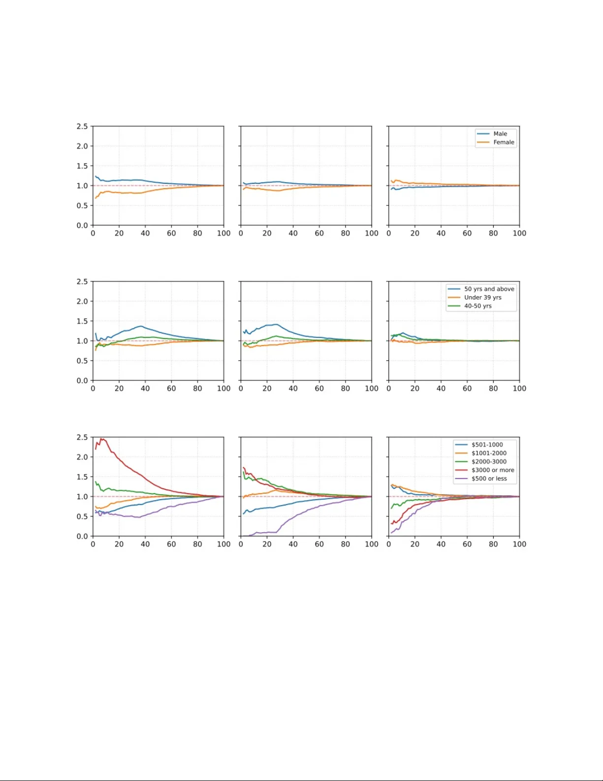
Learning Preference from Observ ed Rankings Y u-Chang Chen National T aiw an Universit y Chen Chian F uh National T aiw an Universit y Shang En Tsai National T aiw an Universit y This V ersion: Jan uary 2026 Abstract Estimating consumer preferences is cen tral to many problems in economics and mark eting. This paper dev elops a ﬂexible framew ork for learning individual preferences from partial ranking information by in terpreting observ ed rankings as collections of pairwise comparisons with logistic c hoice probabilities. W e mo del latent utility as the sum of interpretable pro duct attributes, item ﬁxed eﬀects, and a lo w-rank user-item factor structure, enabling both in terpretability and information sharing across consumers and items. W e further correct for selection in which comparisons are observed: a comparison is recorded only if b oth items enter the consumer’s consideration set, inducing exp osure bias tow ard frequently encoun tered items. W e mo del pair observ ability as the pro duct of item-level observ abilit y prop ensi- ties and estimate these prop ensities with a logistic mo del for the marginal probability that an item is observ able. Preference parameters are then estimated b y maximizing an inv erse-probability-w eighted (IPW), ridge-regularized log-likelihoo d that reweigh ts observ ed comparisons tow ard a target comparison p opulation. T o scale computation, we prop ose a stochastic gradient descent (SGD) algorithm based on in verse-probabilit y resampling, which dra ws comparisons in prop ortion to their IPW weigh ts. In an application to transaction data from an online wine retailer, the metho d improv es out-of-sample rec- ommendation p erformance relative to a p opularity-based b enchmark, with particularly strong gains in predicting purchases of previously unconsumed pro ducts. Keyw ords: incomplete rank data; explo ded logit; inv erse probabilit y weigh ting; ridge regularization. 1 In tro duction Estimating consumer preferences is a foundational task in economics. Preference estimates are cen tral inputs to structural demand and discrete-c hoice mo dels that quan tify substitution patterns and willingness- to-pa y , enabling counterfactual ev aluation of pricing, assortment, and new-pro duct decisions (McF adden, 1973; T rain, 2009). They also underpin stated-preference metho ds such as conjoint and c hoice exp eriments, whic h remain workhorse to ols for pro duct design, p ositioning, and market sim ulation when historical sales data are limited or unav ailable (Green and Sriniv asan, 1990; Louviere, Hensher, and Swait, 2000). In digital mark etplaces, learning preferences at the individual lev el is equally critical for p ersonalization: recommender systems, searc h ranking, and targeted promotions , often lev eraging laten t-factor represen tations and pairwise ranking ob jectiv es (Koren, Bell, and V olinsky, 2009; Koren, Rendle, and Bell, 2021). 1 This paper dev elops a new approac h to learning individual preferences from ranking data. W e consider settings in which researchers observe how consumers rank subsets of av ailable options, rather than complete orderings ov er the en tire choice set. Suc h ranking data may be obtained directly from surv eys that ask resp onden ts to compare or rank alternatives, or indirectly inferred from rev ealed preference in observed c hoices. F or example, if a consumer chooses item j when item j ′ is also a v ailable, this c hoice reveals that j is preferred to j ′ . Crucially , we do not assume that researc hers observe a complete ranking o ver all items for any individual. Instead, the central ob jective of this pap er is to recov er consumers’ underlying preference structures—and, in particular, to infer rankings ov er unobserved item pairs—using only partial and incomplete ranking information observed across individuals. The prop osed approac h learns individual preferences by exploiting tw o complemen tary sources of information. First, preferences can be inferred from ho w consumers rank items with diﬀeren t observ able attributes. Rankings among observed items reveal consumers’ tastes ov er pro duct characteristics, which can then b e extrap olated to items that hav e not b een directly ranked. F or example, if a consumer systematically ranks Brand A ab ov e Brand B among the items she ev aluates, this pattern suggests that pro ducts sharing Brand A’s attributes are likely to b e preferred. Second, the approac h lev erages similarities in observed rankings across consumers. When tw o con- sumers exhibit similar ranking patterns o ver a subset of items, information ab out one consumer’s preferences can inform ab out the other’s unobserved comparisons. In particular, if tw o consumers share closely aligned rankings on a common set of items and one consumer is observed to prefer item A to item B, it is more lik ely that the other consumer also prefers item A to item B. By combining attribute-based extrap olation with cross-consumer similarity , the metho d p ools information eﬃciently to reco ver preferences b eyond the directly observ ed rankings. T o op erationalize these ideas and estimate preferences, we mo del consumers’ latent utility and in- terpret the observed ranking data as a collection of pairwise choice comparisons. The utility of an item is decomposed into an in terpretable comp onent that captures systematic preferences ov er observ able pro d- uct attributes—such as brand or country of origin—and a latent factor component that captures residual similarities b etw een users and items not explained b y these attributes. This structure allows the model to com bine b oth attribute-based extrap olation with information p ooled across consumers who exhibit similar ranking patterns. Estimation pro ceeds b y viewing eac h observed ranking as the outcome of a hypothetical binary c hoice. When item A is observed to b e rank ed ab ov e item B for a given consumer, we interpret this as evidence that the consumer would choose A ov er B if b oth items were simultaneously a v ailable. T o map this interpretation into an estimable likelihoo d, we imp ose the standard assumption that the idiosyncratic utilit y term follo w a t yp e-I extreme v alue distribution. Under this assumption, the probabilit y that item A is preferred to item B tak es a logistic form, and preference estimation reduces to a binary resp onse problem with a logistic speciﬁcation. Because the num b er of implied pairwise comparisons can b e very large, we es- timate the mo del using a sto c hastic optimization pro cedure: in each iteration, we randomly sample a subset of observ ed ranking pairs and up date the parameters using gradient-based steps in the spirit of sto c has- tic gradien t descent. This approach enables scalable estimation while eﬃciently exploiting the information con tained in large and sparse ranking datasets. W e illustrate the prop osed approach using transaction data from an online wine retailer. W e b e- gin by aggregating individual wine pro ducts into interpretable categories deﬁned by region of origin (e.g., Bordeaux), grap e v ariety (e.g., Cab ernet Sauvignon), and price range (e.g., $ 15–30 USD). Based on these categories, we construct customer-sp eciﬁc ranking data from observed purchase b ehavior. Sp eciﬁcally , if a 2 customer has purchased a particular wine category but has not purchased another, w e interpret this pattern as revealing a preference for the purchased category ov er the unpurc hased one. W e then apply our metho d to these constructed rankings to reco ver individual-lev el preference structures. W e assess the practical use- fulness of the approach by ev aluating its out-of-sample predictive p erformance in recommendation tasks. Bey ond prediction, the empirical application also demonstrates ho w the estimated preference rankings can b e translated into actionable managerial insights. In particular, b y computing comp osition and p ercentile lifts from model-implied preferences, w e sho w ho w the framework can inform targeting and segmen tation decisions in mark eting practice. 1.1 Literature Review Econometric analysis of rank data builds on the random utility framew ork: under i.i.d. Type-I extreme v alue errors, a complete ranking admits a rank-ordered (exploded) logit lik eliho o d that factors in to a sequence of m ultinomial logits (Beggs, Cardell, and Hausman, 1981; Chapaaan and Staelin, 1982; Hausman and Ruud, 1987). These rank-based likelihoo ds hav e been used across applied preference measurement settings, rang- ing from parametric unfolding and multic hoice logit mo dels for incomplete rankings to stated-preference designs that translate ordered judgmen ts in to preference and welfare parameters (Calfee, Winston, and Stempski, 2001; DeSarb o, Y oung, and Rangaswam y , 1997; Ophem, Stam, and Praag, 1999). More recen tly , platform search and merchandising environmen ts generate ranking-implied signals through display ed p osi- tions and subsequen t in teractions, motiv ating structural estimation of preferences and ranking p olicies from exp osure-driv en data (Compiani, Lewis, Peng, and W ang, 2024; Negah ban, Oh, and Shah, 2012). A central metho dological theme is unobserv ed heterogeneity in ranking models: mixed-eﬀects sp eciﬁcations introduce random co eﬃcients in rank lik eliho o ds (B¨ oc kenholt, 2001), ﬁnite mixtures and latent classes capture discrete heterogeneit y in ranking patterns (Gormley and Murph y , 2008), and semiparametric approaches relax dis- tributional assumptions while maintaining the random-utilit y structure (Y an and Y o o, 2019). Recen t work further extends these ideas to richer cov ariate structures and mo dern data en vironments (Dong, Han, Jiang, and Xu, 2025). A complementary literature studies preference learning at scale using lo w-dimensional represen ta- tions of unobserved tastes and pro duct attributes. In econometrics and marketing, recent contributions com bine rev ealed-preference inequalities with ﬂexible regularization to enable counterfactual prediction in high-dimensional choice problems (Armona, Lewis, and Zerv as, 2025; Donnelly , Ruiz, Blei, and Athey, 2021; Kallus and Udell, 2016; Magnolﬁ, McClure, and Sorensen, 2025). In parallel, the collaborative-ﬁltering lit- erature estimates user and item embeddings from implicit feedback using pairwise ranking ob jectives with a logistic form for utilit y diﬀerences, typically optimized via sto chastic gradient metho ds (He and McAuley, 2016; Oh, Thekumparampil, and Xu, 2015; Rendle, Gantner, F reudenthaler, and Sc hmidt-Thieme, 2011). While often presen ted as algorithmic, these approaches are conceptually compatible with random utility mo dels based on pairwise comparisons. Our pap er integrates these strands by embedding a lo w-rank latent factor structure within an econometric logit likelihoo d for observed (and incomplete) rankings, where the set of observ ed comparisons can itself be selected b ecause exposure depends on platform ordering, pro duct p opu- larit y , or prior p ersonalization. W e address this endogenous observ ability using in verse probabilit y weigh ting (IPW), rew eighting eac h observed comparison b y its estimated exp osure prop ensity to reco ver preference pa- rameters under standard selection-on-observ ables conditions. This correction parallels prop ensity-w eighted debiasing in recommendation and learning-to-rank, which treats display ed rankings as treatments and uses in verse-propensity weigh ts to obtain un biased learning from biased feedbac k (Joac hims, Swaminathan, and 3 Sc hnab el, 2017; Schnabel, Sw aminathan, Singh, Chandak, and Joachims, 2016). 2 Metho d 2.1 Observ ed Rankings W e assume that researc hers observe rankings o ver a set of items j = 1 , 2 , . . . , m for individuals i = 1 , 2 , . . . , n . Let ⪰ i denote the (latent) preference relation of individual i , where j 1 ⪰ i j 2 indicates that individual i prefers item j 1 to item j 2 . Imp ortantly , w e allow the observed ranking information to b e incomplete: for eac h individual, preferences are only observ ed for a subset of item pairs. It is useful to visualize the observed ranking information for an individual as a matrix. F or illustration, consider the case with m = 5 items. The observed rankings for individual i can b e represented b y the follo wing upp er-triangular matrix R i : R i =         − ⪰ · ⪰ · − ⪰ · · − · ⪰ − · −         , where an en try ⪰ in p osition ( j 1 , j 2 ) indicates that the comparison j 1 ⪰ i j 2 is observed, and · denotes that the ranking b et ween the tw o items is unobserved. Diagonal elements are omitted since self-comparisons are not meaningful. F ormally , let D i = { ( j 1 , j 2 ) | j 1 ⪰ i j 2 } denote the set of observed pairwise rankings for individual i . W e do not require the same items, or the same item pairs, to b e rank ed by all individuals; consequently , the in tersection ∩ n i =1 D i ma y b e empt y . F ollo wing standard assumptions, we assume that each individual’s observ ed preference relation ⪰ i is transitiv e, while allo wing it to b e incomplete b ecause only a subset of pairwise comparisons is observed for eac h individual. Let D = { ( i, j, j ′ ) | ( j, j ′ ) ∈ D i } denote the collection of all observ ed rankings across individuals. This set constitutes the data used for estimation, and our primary ob ject of interest is to infer the unobserved preferences ( i, j, j ′ ) / ∈ D that are not directly observed in the data. In practice, observ ed rankings may arise from several sources. One common source is survey data in whic h individuals are asked to rank or compare a subset of items; how ever, eliciting complete rankings is often infeasible when the choice set is large. Rankings ma y also b e constructed from rating data by conv erting n umerical ratings in to ordinal comparisons, though such rankings are typically incomplete b ecause individuals do not rate all a v ailable items. A third and particularly important source is rev ealed preference inferred from observ ed choices. F or example, if an individual consumes certain items (e.g., watc hes a movie on Netﬂix) but not others, this behavior can b e interpreted as rev ealing a preference for the consumed items ov er those not c hosen. In our empirical application, we construct the ranking data D from transaction records provided by an online wine retailer. Sp eciﬁcally , we in terpret wine A as being preferred to wine B for a giv en consumer if the consumer has purchased wine A but has not purchased wine B during the observ ation p erio d. 4 2.2 Mo deling Utilit y F unction F ollowing the random utility framework (McF adden, 1973), w e assume that the observ ed rankings are gen- erated from the latent utility u ij = x ⊤ j β i + α j + λ ⊤ i f j + ε ij , where x j is a v ector of observed pro duct attributes, α j is an item ﬁxed eﬀect capturing global p opularity or a verage p erceived qualit y , and ε ij is an idiosyncratic utility sho c k that reﬂects unobserv ed factors aﬀecting individual i ’s ev aluation of item j . W e allow preferences ov er observ able attributes to b e heterogeneous across individuals b y p ermitting the coeﬃcient v ector β i to v ary at the individual level. In addition to observ able attributes, the utility speciﬁcation includes a laten t factor f j ∈ R r that captures unobserved characteristics of item j , where the dimension r is chosen by the researcher. Depending on the application, these laten t characteristics may represent asp ects such as ov erall st yle, quality gradients, usage o ccasions, or other dimensions of diﬀerentiation that are not directly measured in the data. In our empirical application using wine transactions, f j ma y capture unobserv ed attributes such as the prestige asso ciated with certain regions or stylistic features related to the taste of the wine that are not fully summa- rized by observed lab els. The corresp onding factor loadings λ i are individual-sp eciﬁc, allo wing consumers to diﬀer in ho w they v alue these latent characteristics. The inclusion of latent factors allows the mo del to capture systematic dep endence in utilit y across individuals and items b eyond what is explained by observed attributes and ﬁxed eﬀects. Items that tend to b e ranked similarly by many consumers will acquire similar laten t represen tations, while consumers who exhibit comparable ranking patterns will load similarly on these latent dimensions. As a result, information ab out preferences can b e shared across individuals and across items, enabling the mo del to infer unobserv ed comparisons by exploiting common structure in ranking b eha vior rather than treating each consumer–item ev aluation in isolation. W e estimate the mo del by interpreting the observed rankings D as a collection of binary choice problems. Sp eciﬁcally , when we observe that individual i ranks item j ab ov e item j ′ , we interpret this observ ation as revealing that, if both items were av ailable sim ultaneously , individual i would choose item j o ver item j ′ . Let θ = { β i , α j , λ i , f j } i =1 ,...,n ; j =1 ,...,m denote the set of mo del parameters, and assume that the idiosyncratic utility sho c ks ε ij follo w the type-I extreme v alue distribution. Under this assumption, the probability that individual i prefers item j to item j ′ tak es the logistic form P ( j ⪰ j ′ | θ ) = σ ( u ij − u ij ′ ) = 1 1 + exp[ − ( u ij − u ij ′ )] , where σ ( x ) = 1 1+exp( − x ) denotes the sigmoid function. Giv en the pairwise-choice interpretation, each observed comparison ( i, j, j ′ ) ∈ D contributes a likeli- ho o d term equal to the probabilit y that individual i prefers item j to item j ′ . Under the logistic speciﬁcation deriv ed ab ov e, the likelihoo d contribution of a single observed pair is σ ( u ij − u ij ′ ). Assuming indep endence of the idiosyncratic utilit y sho cks across individuals and items, the log-lik eliho o d of the full dataset D is 5 giv en by: ℓ ( θ | D ) = X ( i,j,j ′ ) ∈D ln σ ( u ij − u ij ′ ) , whic h corresp onds to the ob jective function used for estimation. 2.3 Correcting for Selection in Observ ability The lik eliho o d in Section 2.2 treats the observed comparison set D as if it were a representativ e sample of the underlying pairwise preference relation. In many ranking applications, how ever, whic h comparisons are observ ed is itself selected. W e refer to this phenomenon as selection in observ ability: a pairwise comparison b et ween items j and j ′ is recorded only when b oth items are simultaneously av ailable to, encountered by , or considered b y the individual. Selection in observ ability is p erv asive in practice. Survey resp ondents can rank only a limited num b er of items; in rating or consumption data, items are observ ed only if they are encountered; and in digital commerce, exp osure is shap ed b y platform searc h, recommendations, assortment constraints, sto ck outs, and time-v arying promotions. As a result, comparisons inv olving highly visible items are ov errepresented, while comparisons inv olving niche or infrequently a v ailable items are systematically missing. Ignoring this selection can bias preference estimates by conﬂating exp osure with taste. a concern that is closely related to consideration-set formation in mark eting and exposure bias in recommender systems (Hauser and W ernerfelt, 1990; Joac hims et al., 2017; Roberts and Lattin, 1991; Schnabel et al., 2016). T o formalize selection in observ ability , let O ij j ′ ∈ { 0 , 1 } denote an indicator that the comparison b et ween items j and j ′ is observable for individual i . W e interpret O ij j ′ = 1 as the ev ent that b oth items en ter the individual’s eﬀectiv e consideration or a v ailability set (e.g., both app ear in the surv ey task or both are encoun tered through search and recommendation). The observed pairwise dataset D can b e view ed as the collection of comparisons for which observ ability holds and an ordering is recorded: ( i, j, j ′ ) ∈ D ⇒ O ij j ′ = 1 and w e observe that j ⪰ i j ′ . Let π ( x j ) ∈ (0 , 1) denote the (marginal) probabilit y that item j is observ able as a function of item-side ob- serv ables x j . W e assume that, conditional on observ ables, the probability that a pair is observ able factorizes as π j j ′ = Pr( O ij j ′ = 1 | x j , x j ′ ) = π ( x j ) π ( x j ′ ) ≡ π j π j ′ . This assumption captures the idea that observ ability is primarily driven by item-level exp osure or av ailability , and implies that rarely av ailable items mechanically generate few er observ ed comparisons with an y other item. As detailed in the next subsection, we will adopt in verse probability weigh ting (IPW) based on estimates of π ( · ) to adjust for selection in observ ability . 2.4 Estimation and Computation Optimizing the likelihoo d function p oses sev eral tec hnical c hallenges. First, the model is high-dimensional, as it includes b oth individual-sp eciﬁc parameters ( β i , λ i ) and item-sp eciﬁc parameters ( α j , f j ). Such high dimensionalit y can lead to numerical instability and noisy estimates, particularly in settings with sparse ranking data. Second, the cardinality of D can b e very large, since it contains all observed pairwise com- parisons implied b y the rankings. Directly optimizing the likelihoo d using the full dataset D is therefore 6 computationally demanding. T o address the ﬁrst challenge, w e in tro duce regularization into the estimation pro cedure. Let Θ denote the parameter space. W e estimate θ by minimizing an IPW-corrected p enalized negative log-lik eliho o d: ˆ θ = arg max θ ∈ Θ X ( i,j,j ′ ) ∈ D 1 ˆ π j j ′ ln σ ( u ij − u ij ′ ) − κ ∥ θ ∥ 2 2 , where κ > 0 is the penalty term and ˆ π j j ′ is the estimate of the probability that the comparison betw een j and j ′ is observed. The in verse-probabilit y weigh ting 1 ˆ π j j ′ corrects for selection by upw eighting under-considered pairs (Horvitz and Thompson, 1952; Rosenbaum and Rubin, 1983). Rather than estimating a separate prop ensit y for each unordered pair { j, j ′ } , which is infeasible when m is large, w e exploit the factorization and imp ose a parsimonious parametric mo del on the marginal observ ability probability . Speciﬁcally , we parameterize π j ≡ π ( x j ; ψ ) = σ ( x ⊤ j ψ ) , where ψ is an auxiliary parameter v ector (distinct from the preference parameters θ ) and x j includes an in tercept. This sp eciﬁcation plays the role of a prop ensit y-score mo del: it maps item-side observ ables into a probabilit y that item j enters the consideration/observ ability pro cess, and it induces the pairwise comparison probabilit y π j j ′ = π ( x j ; ψ ) π ( x j ′ ; ψ ). T o estimate ψ using based on whic h comparisons are observed, we construct, for every individual i and unordered pair { j, j ′ } , the observ ability indicator O ij j ′ = 1 { ( i, j, j ′ ) ∈ D or ( i, j ′ , j ) ∈ D } . Under the imp osed mo del, O ij j ′ is a Bernoulli random v ariable with success probabilit y π j j ′ ( ψ ) = π ( x j ; ψ ) π ( x j ′ ; ψ ). Let N j j ′ = P n i =1 O ij j ′ denote the num b er of individuals for whom the unordered pair { j, j ′ } is observed. The resulting (aggregated) log-likelihoo d for ψ is ℓ O ( ψ ) = X 1 ≤ j 0 is the learning rate. Computationally , the SGD algorithm can b e implemented without scanning all elements of D b ecause ˆ π j j ′ dep ends only on the pair { j, j ′ } . W e precompute ˆ π j j ′ for each observed pair and main tain, for each pair, the list of indices in D that corresp ond to that pair. W e then (i) sample an unordered pair { j, j ′ } using an alias table with weigh ts prop ortional to ˆ π − 1 j j ′ |D j j ′ | , where |D j j ′ | is the num b er of observ ed comparisons in D inv olving { j, j ′ } , and (ii) sample uniformly from the stored indices within D j j ′ to obtain a triple ( i, j, j ′ ). This tw o-stage procedure yields exact draws for optimizing the ob jective function while preserving the p er-iteration cost of standard SGD. 3 Empirical Illustration 3.1 Data and Bac kground W e illustrate the prop osed preference-learning framework using proprietary transaction data from a leading online alcoholic-b everage retailer in T aiwan, cov ering all orders placed on the platform betw een 2021 and 2024. While the retailer oﬀers a broad p ortfolio of alcoholic pro ducts—including sake and whisky—wine constitutes its core category in terms of b oth sales volume and pro duct v ariety . T o maintain a fo cused empirical setting, w e therefore restrict atten tion to wine purchases throughout the analysis. The dataset comprises 311,089 transaction records from 23,721 unique customers. Each transaction is link ed to a p ersistent customer identiﬁer, allowing us to reconstruct individual purc hase histories o ver time. F or every order, we observ e the transaction timestamp, a unique pro duct identiﬁer, quantit y purchased, and price paid, along with detailed pro duct attributes such as country of origin, region, color, sweetness level, vin tage, and b ottle size. In addition, self-reported demographic information—including age and gender—is a v ailable for a subset of customers. T ak en together, these data form a ric h panel of consumer–pro duct in teractions: the detailed attribute information supports a structured representation of wine characteristics, while the longitudinal purchase histories allo w us to infer relativ e preferences from revealed choice b ehavior. This com bination makes the setting particularly w ell suited for studying heterogeneous preferences using ranking-based metho ds. T able 1 rep orts customer-level summary statistics for all customers who made at least one purchase during the 2021–2024 perio d. The customer base is slightly male-skew ed (59.7%) with an av erage age of appro ximately 40. Annualized spending a verages 10,322 NTD (USD 323), but the distribution is highly righ t-skew ed (SD 37,945 NTD; USD 1,186), indicating a small group of hea vy buy ers. Customers purc hase relativ ely infrequen tly—2.65 orders per y ear on av erage—implying eac h transaction is sizable, consisten t with o ccasional, high-inv olvemen t purchases. In terms of pro duct comp osition, preferences tilt strongly tow ard Old W orld wines: 63% of customers purc hase F rance at least once, and 84.7% purc hase from Old W orld 8 regions o verall. 1 Nev ertheless, New W orld wines are also common, with 50% of customers purc hasing at least one b ottle. Finally , participation is concen trated in the lo w and mid price tiers—deﬁned as 500–1,000 NTD (USD 16–31) and 1,001–3,000 NTD (USD 31–94), resp ectiv ely—with 61% and 66% of customers purchasing at least once in these ranges. By con trast, only 9% of customers ever purc hase high-end wines, deﬁned as prices ab ov e 10,000 NTD (USD 313+). These patterns motiv ate a mo deling approach that allows for substan tial heterogeneity in both origin preferences and price sensitivit y . 3.2 Construction of Ranking Data T o address the extreme sparsity inherent in transaction-level wine data, we aggregate individual sto ck- k eeping units (SKUs) in to economically meaningful wine categories. This aggregation is designed to reduce dimensionalit y while preserving the attributes most relev ant for consumer diﬀerentiation. The resulting represen tation reﬂects extensive consultation with domain experts from the retailer and balances statistical tractabilit y with interpretabilit y . W e b egin by standardizing raw pro duct information to obtain a consistent description of each wine. The catalog rep orts a four-lev el geographic hierarch y (country , ma jor region, app ellation, and sub-app ellation), and wine color (e.g., red, white). T o mitigate sparsity at ﬁne geographic levels, we collapse the hierarc hy to coun try (e.g., F rance) and ma jor region (e.g., Bordeaux) , and drop the more granular sub-app ellation level (e.g., the Pauillac village in Bordeaux). This choice retains the primary origin distinctions that consumers commonly use in ev aluating wines, while a voiding categories that are to o sparsely p opulated for reliable estimation. Next, we discretize prices into tiers in tended to capture meaningful diﬀerences in consumer sp ending b eha vior rather than arbitrary n umeric cutoﬀs. Guided b y the retailer’s domain knowledge and industry exp erience,, we deﬁne the following price tiers: up to 500 NTD; 501–1,000; 1,001–2,000; 2,001–3,000; 3,001– 4,000; 4,001–5,000; 5,001–10,000; 10,001–20,000; and ab ov e 20,000 New T aiwanese Dollar (NTD). 2 This discretization preserves v ertical diﬀerentiation in price while reducing noise from idiosyncratic pricing and infrequen tly purchased premium SKUs. In parallel, w e standardize wine st yles using a rule-based taxonomy designed to reduce heterogeneity arising from inconsisten t grap e-v ariety nomenclature and ov erly granular blend deﬁnitions. Grap e v ariety names are ﬁrst standardized b y merging synon yms and region-speciﬁc aliases, after which eac h wine is assigned an initial style label based on the set of grap e v arieties used, abstracting from blending prop ortions. Within each region, styles are ranked by pro duct prev alence, with those collectively accoun ting for the top 80% of pro ducts classiﬁed as ma jor styles; remaining low-frequency st yles are treated as minor and collapsed in to broader “red wine” or “white wine” categories. Ma jor styles are then mapped to a set of canonical global wine styles (e.g., the “Bordeaux Blend” style that mainly comp oses of Cab ernet Sauvignon and Merlot) using predeﬁned rules linking grap e-v ariety combinations to widely recognized style labels. Wines that do not matc h an y canonical rule retain their original v ariety-based lab els. A detailed description of the taxonomy and mapping rules is provided in App endix Section 6.1. W e then combine origin (country– region–app ellation), grap e v ariety , and price tier to deﬁne a comp osite product segmen t for each wine. F or example, a red wine from F rance, Bordeaux, Pauillac priced at 2,300 NTD is classiﬁed as “F rance–Bordeaux, 1 In the wine context, Old World refers to traditional Europ ean wine-producing regions such as F rance, Italy , Spain, and Germany , while New World refers to pro ducers outside Europe, including the United States, Chile, Australia, New Zealand, and South Africa. 2 Using an exc hange rate of 1 USD = 32 NTD, these cutoﬀs corresp ond to approximately USD 16, 31, 63, 94, 125, 156, 313, 625, and ab ov e USD 625. 9 T able 1: Customer Summary Statistics Av erage SD Min Max A. Demo gr aphics F emale 0.428 0.495 0 1 Age (y ears) 39.93 11.09 18 83 B. Pur chase Behavior (A nnualize d) Sp ending (NTD) 10,322 37,945 166 1,120,101 Sp ending (USD) 323 1,186 5.1 35,003 Purc hase F requency 2.65 7.41 0.25 158.86 C. R e gion ever Pur chase d F rance 0.63 0.48 0 1 Italy 0.38 0.48 0 1 US 0.22 0.41 0 1 Old W orld 0.847 0.36 0 1 New W orld 0.50 0.5 0 1 D. Wine T yp e ever Pur chase d Red Wine 0.71 0.45 0 1 White Wine 0.50 0.5 0 1 Sparkling 0.31 0.46 0 1 E. Pric e Tier ever Pur chase d (in USD) Lo w Price ( ≤ 31) 0.61 0.49 0 1 Mid Price (31 – 94) 0.66 0.47 0 1 Mid-High Price (94 – 313) 0.28 0.44 0 1 High Price ( ≥ 313) 0.09 0.29 0 1 Note: The unit of observ ation is customer. The sample consists of 23 , 721 observ a- tions; Panel A reports demographics for customers who made at least one purchase during the 2021–2024 sales p erio d. Panel B rep orts annualized purchase b ehavior, where sp ending, purchase frequency , and items purchased are a veraged across the four-y ear sample perio d. Panel C–E reports purc hase propensities based on indicator v ariables for whether a customer purc hased at least one b ottle from the corresp ond- ing origin group, wine type, or price tier during the sample p erio d, whose indicate the share of customers with the indicator equal to one. 10 Bordeaux Blend, 2,001–3,000.” In all subsequen t analysis, these comp osite pro duct segments are treated as the “items” in the mo del. Finally , w e construct a set of observ ed pairwise rankings that enco de rev ealed preferences at the customer level as the following. F or a giv en customer i , item j is said to b e preferred to item j ′ if the customer purchased at least one wine b elonging to item j during the sample p erio d but did not purc hase an y wine b elonging to item j ′ . Each such comparison is in terpreted as a rev ealed preference statement that j ≻ u j ′ . F ormally , the dataset D consists of all observ ed triplets ( i, j, j ′ ) satisfying this condition. The collection D therefore aggregates, for each customer, a set of pairwise comparisons b etw een purc hased and unpurc hased items. These comparisons form an incomplete but informative ranking o ver the item space, reﬂecting relativ e preferences inferred from observ ed purchase b ehavior. 3.3 Mo del Sp eciﬁcaiton Because each item j is deﬁned as a comp osite of region ( r ), grap e v ariety ( g ), and price tier ( p ), it is con venien t to index items b y the triple ( r, g , p ). W e denote the latent utility that individual i derives from item ( r , g , p ) b y u irg p . T o capture preferences o ver observ ed pro duct characteristics while preserving the collab orativ e-ﬁltering adv antages of the metho d, w e sp ecify the utility function as u irg p = δ r + γ g + π p + λ ⊤ i f rg p + ε irg p , (1) where δ r is a region ﬁxed eﬀect, γ g is a grape-v ariety ﬁxed eﬀect, and π p is a price-tier ﬁxed eﬀect. These comp onen ts join tly summarize the contribution of observed pro duct attributes to utility . The idiosyncratic error term ε irg p captures unobserved taste sho cks and is assumed to follo w a type-I extreme v alue distribution. The term λ ⊤ i f rg p represen ts the laten t factor component of the mo del. Here λ i is an individual-speciﬁc preference v ector and f r,g,p is a laten t feature vector associated with item ( r, g , p ). These latent dimensions capture aspects of pro duct v aluation that are not directly observed in the data but systematically inﬂuence c hoice. In the wine con text, they may reﬂect preferences o ver abstract attributes such as perceived prestige, taste, or a preference for certain ﬂa vor proﬁles that cut across formal grape or price classiﬁcations. They ma y also absorb con text-sp eciﬁc demand factors, suc h as whether purc hases are intended for gifting or celebration v ersus routine consumption. By conditioning on observed attributes (region, grap e v ariety , and price tier) and augmenting them with a ﬂexible latent factor structure, the model accommo dates rich heterogeneity in preferences while preserving interpretabilit y along economically meaningful dimensions. The factor structure also enables the model to learn similarity patterns from co-purchase b ehavior. Consumers who exhibit similar ranking patterns ov er observed items are placed nearby in the latent pref- erence space, while items that tend to b e purchased by similar sets of consumers acquire similar latent represen tations. This data-driv en embedding allo ws the model to extrap olate preferences to unobserved items and to capture substitution patterns that are not fully explained by observ able pro duct characteristics alone. 3.4 Estimation Results W e b egin by summarizing the distribution of estimated region-sp eciﬁc preference eﬀects across consumers. T o provide a compact and interpretable view of preference heterogeneity , we focus on six representativ e wine regions that span b oth the Old W orld and the New W orld: Bordeaux and Burgundy (F rance), California (United States) and Cen tral V alley (Chile), South Australia (Australia), and Marlb orough (New Zealand). 11 F or each region, Figure 1 plots the empirical distribution of the individual-sp eciﬁc region co eﬃcients δ r,i , whic h capture how strongly a given consumer ranks wines from region r relative to other regions, holding grap e v ariety and price tier ﬁxed. (a) Bordeaux (b) Burgundy (c) California (d) South Australia (e) Central V alley (f ) Marlb orough Figure 1: Distributions of individual-sp eciﬁc region eﬀect coeﬃcients δ r for the six regions. In Figure 1, several patterns emerge. First, historically prestigious and widely consumed regions suc h as Bordeaux and Burgundy exhibit distributions that are shifted right w ard relative to other regions, indicating higher a verage preference lev els and a substan tial mass of consumers with strongly positive region- sp eciﬁc utility . A t the same time, these distributions are clearly disp ersed and often bimo dal, revealing pronounced heterogeneit y . In con trast, regions with more sp ecialized or stylistically distinctiv e proﬁles—suc h as Marlb orough—displa y distributions that are more tightly concentrated around zero with thinner righ t tails, suggesting a narrow er but more homogeneous app eal. T aken together, these results indicate that regional origin op erates not merely as a mean-shifting attribute but as a salient dimension of preference heterogeneit y , underscoring the imp ortance of allowing region eﬀects to v ary ﬂexibly across individuals. W e insp ect correlation b etw een regional preference in Figure 2. Two patterns stand out. First, the three New W orld regions (California, South Australia, and Central V alley) exhibit the strongest p ositiv e co- mo vemen t in preferences. This clustering suggests that relativ e aﬃnity for one of these regions also tend to displa y higher aﬃnit y for the others. Second, the t wo F rench b enchmark regions (Bordeaux and Burgundy) are p ositively correlated, but only mo destly (0 . 10), indicating that “liking F rance” is not a dominant single dimension of heterogeneity once the model accounts for other pro duct characteristics. Moreov er, the correla- tions b etw een the F rench regions and some New W orld regions are slightly negative (e.g., Bordeaux–Central V alley: − 0 . 05), consisten t with mild substitution in rankings b et ween these styles for some customers. Finally , Marlb orough, which is most known for Sauvignon white wines, appears relatively distinct: its correlations with the New W orld cluster are near zero and remain small ev en with South Australia. W e next examine heterogeneity in price-related preferences b y turning to the estimated price-tier co eﬃcien ts π p . Figure 3 reports the distribution of individual-sp eciﬁc co eﬃcients for each price range. Sev eral features closely parallel the patterns observed for region eﬀects. Most notably , the mass-market tiers 12 Figure 2: Correlation matrix of customer-sp eciﬁc region preference eﬀects. Eac h en try rep orts the pairwise correlation b etw een tw o regions’ preference eﬀects. 13 (NTD 501–1,000 (USD 16–31) and NTD 1,001–2,000 (USD 31–63)) exhibit pronounced bimo dality . As in the case of p opular regions such as Bordeaux and Burgundy , these distributions reveal tw o sizable groups of consumers with opp osing preference. In contrast, higher price tiers (ab ov e NTD 2,001 (USD 63)) displa y distributions dominated by a negative mo de with a small but persistent p ositive right tail. This mirrors the region results for more nic he or sp ecialized origins, where av erage app eal is limited but a minority segmen t exhibits strong p ositiv e v aluation. At the very top end (NTD 10,001 and ab ov e), the distributions b ecome more concen trated and closer to unimo dal, reﬂecting a narrow er eﬀective choice set and stronger regularization arising from sparse interactions. (a) NTD ≤ 500 (b) NTD 501–1,000 (c) NTD 1,001–2,000 (d) NTD 2,001–3,000 (e) NTD 3,001–4,000 (f ) NTD 4,001–5,000 (g) NTD 5,001–10,000 (h) NTD 10,001–20,000 (i) NTD > 20,000 Figure 3: Distributions of user-sp eciﬁc price-tier co eﬃcients. Each panel sho ws the estimated co eﬃcient distribution for one price tier in the ranking mo del. Using an exchange rate of 1 USD = 32 NTD, these cutoﬀs corresp ond to approximately USD 16, 31, 63, 94, 125, 156, 313, 625, and ab o ve 625. Figure 4 rep orts the correlation matrix of the estimated price-tier co eﬃcients. Tw o broad patterns 14 stand out. First, preferences across higher price tiers exhibit a clear blo ck structure: adjacent premium tiers are strongly p ositively correlated, with correlations around 0 . 48–0 . 52 for neighboring ranges (e.g., NTD 3,001–4,000 vs. 4,001–5,000, and 4,001–5,000 vs. 5,001–10,000). This indicates that consumers who v alue premium wines tend to substitute within a narrow band of nearby price tiers rather than fo cusing on a single exact price p oin t. Correlations decay quickly as price distance increases, suggesting that price-related preferences are organized around lo cal consideration sets rather than a single smo oth ranking ov er the entire price sp ectrum. Second, the mass-mark et tier NTD 501–1,000 pla ys a distinct role. Its co eﬃcients are negatively correlated with most mid- and high-price tiers (e.g., ρ = − 0 . 35 with NTD 2,001–3,000 and ρ = − 0 . 29 with NTD 3,001–4,000), indicating that this range acts as a dividing line in consumers’ price preferences. One group systematically fav ors wines in this range while do wn-weigh ting higher tiers, whereas another group do es the opp osite. By contrast, the very low-price tier (b elow NTD 500) is weakly correlated with most tiers and even mildly p ositively correlated with the highest price ranges. This pattern suggests that sub-500 purchases often co exist with premium buying—reﬂecting add-on, trial, or casual-o ccasion purchases rather than a strictly low-budget orientation. Ov erall, the correlation structure reinforces the distributional evidence: price preferences are b est described by discrete segmentation of consideration sets, esp ecially around the NTD 501–1,000 threshold, with a coherent premium block c haracterized b y substitution among neigh b oring high-price tiers. Figure 4: Correlation matrix of price preference eﬀects. Each entry rep orts the pairwise correlation across customers betw een t wo price-tier preference eﬀects. Prices sho wn in the ﬁgure are in NTD. Using an exc hange rate of 1 USD = 32 NTD, these cutoﬀs correspond to approximately USD 16, 31, 63, 94, 125, 156, 313, 625, and ab ov e 625. 15 4 Application I: Recommender System 4.1 Recommender System W e ﬁrst ev aluate the proposed framework in a recommendation setting that fo cuses explicitly on predicting the purc hase of new items—that is, wine categories a customer has not previously consumed. This task is of direct managerial relev ance: eﬀectiv e recommendations should help customers discov er new pro ducts rather than merely rep eat past purchases. A t the same time, predicting new-item adoption is empirically c hallenging because it requires extrap olating preferences b eyond observed consumption histories, esp ecially in mark ets with highly diﬀeren tiated pro ducts and sparse individual-level purchase data. A key adv antage of a ranking-based preference mo del is precisely its ability to infer relative preferences o ver unobserv ed items b y combining information from observ able attributes and cross-consumer similarity . Based on the estimated mo del parameters ˆ θ = ( ˆ δ r , ˆ γ g , ˆ π p , ˆ λ i , f rg p ), we construct predicted utility scores for eac h consumer–item pair, ˆ u irg p = ˆ δ r + ˆ γ g + ˆ π p + ˆ λ ⊤ i ˆ f rg p , whic h summarize the mo del-implied relative preference for item ( r , g , p ) b y consumer i . Recommendations are generated by ranking all candidate items according to these predicted scores. F or each consumer, w e select the top- N items with the highest predicted utility . T o fo cus on gen uine out-of-sample prediction, w e exclude from the candidate set an y items the consumer has previously purchased. The resulting task therefore ev aluates the mo del’s abilit y to rank and recommend pr eviously untrie d pro duct categories, rather than its abilit y to recov er observed choices. Finally , recommendations are constructed at the pro duct-category level rather than at the level of individual sto ck keeping units. This design choice mirrors the construction of the ranking data used for esti- mation, where user preferences are mo deled o ver interpretable wine categories deﬁned by region, grap e v ari- et y , and price tier. Operating at this lev el allows the model to recommend no vel but related products—such as wines from a familiar region or st yle at a diﬀeren t price p oin t—thereby aligning the recommendation exercise with the underlying preference-learning ob jective. 4.2 Ev aluation Metho ds T o ev aluate out-of-sample recommendation p erformance, w e split the transaction data into training and test sets using a time-aw are cross-v alidation procedure. The split is constructed to b e strictly disjoin t at the transaction level to preven t information leak age. In addition, purchase b ehavior in wine mark ets is sub ject to pronounced short-term cycles arising from seasonality , promotional campaigns, and time-sp eciﬁc pro duct a v ailability . F or example, Beaujolais Nouv eau is released annually in Nov ember and is typically accompanied by in tensive, short-lived marketing campaigns that generate sharp and predictable demand spik es. 3 T o account for these features of the data, w e adopt a splitting strategy that preserves local temp oral structure while a voiding systematic distributional diﬀerences b et ween the training and test samples. Sp eciﬁcally , w e implement a w eekly leav e-one-day-out sc heme. F or eac h calendar w eek in the sample p erio d, one weekda y is randomly selected and all transactions o ccurring on that day are assigned to the 3 Beaujolais Nouveau is traditionally released on the third Thursda y of Nov ember each year. Retailers often co ordinate concentrated promotions and limited-time oﬀerings around the release date, leading to highly lo calized surges in purchases that are not representativ e of underlying, stable preferences. 16 test set, while transactions from the remaining six days of the same week form the training set. This pro cedure is applied indep endently for every week. By construction, the test set draws observ ations from all weekda ys across the sample p erio d, ensuring that ev aluation results are not driv en by particular days, promotional schedules, or recurring weekly patterns. T o mak e the ev aluation exercise feasible, we restrict atten tion to customers and items that app ear in b oth the training and test samples. If a consumer or pro duct category app ears only in one split, out-of-sample prediction is unav ailable b ecause the mo del cannot generate meaningful preference rankings for that unit. Lik ewise, if a customer app ears only in the training data, no out-of-sample ev aluation is possible because there are no held-out purc hases against whic h predicted rankings can b e assessed. Recommendation quality is ev aluated using Precision@ K and Recall@ K , where K denotes the length of the recommendation list. Both metrics are designed to assess the mo del’s ability to predict purchases of previously unconsumed pro duct categories. W e b egin by deﬁning the relev ant consumer-sp eciﬁc sets. F or a given consumer i , let A i denote the gr ound-truth set of newly purc hased pro duct categories in the test data—that is, categories j = ( r , g , p ) that app ear in the consumer’s test data but were not observ ed in the training data. F ormally , A i = { j = | j ∈ T est i ∧ j / ∈ T rain i } . This set captures the consumer’s newly revealed preferences during the ev aluation window. Also, let B ( K ) i denote the r e c ommendation set , deﬁned as the top- K pro duct categories rank ed by the mo del for consumer i , after excluding all categories previously observed in the training data: B ( K ) i = { j i 1 , j i 2 , . . . , j iK } . The in tersection A i ∩ B ( K ) i therefore represen ts hits —categories that are b oth recommended b y the mo del and subsequen tly purchased b y the consumer in the test data. Using these deﬁnitions, Recall@ K is deﬁned as Recall@ K =    A i ∩ B ( K ) i    |A i | , (2) whic h measures the extent to which the recommendation list recov ers the consumer’s newly expressed pur- c hase interests. The second ev aluation metric Precision@ K is deﬁned as Precision@ K =    A i ∩ B ( K ) i    K , (3) whic h is the fraction of recommended items that are subsequently v alidated by observ ed purchases. Precision@ K therefore captures ranking accuracy at the top of the recommendation list. Both metrics are computed at the consumer lev el and then a veraged across customers to obtain aggregate p erformance measures. 4.3 Results W e ev aluate the recommendation p erformance of the prop osed mo del and assess whether com bining attribute- based preference comp onents with latent factor learning yields meaningful gains in out-of-sam ple prediction. All ev aluations are conducted at the consumer level using held-out purchase data, following the training and 17 testing proto col describ ed in Section 4.2. P erformance is measured using Precision@ K and Recall@ K , and statistical signiﬁcance is assessed via paired tests based on consumer-level metric diﬀerences. Our primary b enchmark is a popularity-based recommender that ranks product categories b y their o verall purc hase frequency in the training data. This b enchmark reﬂects a realistic managerial practice in settings where individual-lev el information is unav ailable, incomplete, or too costly to op erationalize. In such cases, recommending the most p opular items is a simple, low-cost strategy that requires no p ersonalization infrastructure and is therefore easy to adopt in practice. Ho wev er, b ecause it deliv ers the same recommenda- tion list to all consumers, this approac h ignores heterogeneit y in preferences, it ma y b e ineﬃcien t when tastes are diverse. Comparing our mo del against this b enc hmark allows us to quantify the incremental v alue of p ersonalization—namely , the extent to which exploiting individual-level preference information can improv e recommendation accuracy . In addition to this b enchmark, we consider tw o restricted v ariants of our mo del to isolate the sources of predictive p erformance. The ﬁrst v ariant relies exclusiv ely on observed pro duct attributes—region, grape v ariety , and price tier—captured b y the ﬁxed-eﬀect comp onents ( δ r , γ g , π p ), and therefore exploits only systematic, interpretable diﬀe rences across pro ducts. The second v ariant relies solely on the laten t factor structure ( λ i , f rg p ), abstracting from all observ able attributes and capturing preference similarity through collab orativ e patterns alone. Comparing these restricted sp eciﬁcations to the full model allo ws us to assess whether predictive gains arise from one comp onent in isolation or from their in teraction. As we show b elow, neither attributes nor latent factors alone are suﬃcient to matc h the p erformance of the full mo del; rather, it is the combination of structured pro duct information and data-driven laten t heterogeneity that delivers the strongest recommendation accuracy . T able 2 rep orts recommendation p erformance across diﬀerent list lengths. First note that p opularity- based b enchmark in fact performs reasonably well, as the wine mark et is high-concen trated in T aiwan: a small num b er of well-kno wn regions and styles—suc h as Bordeaux and Burgundy—account for a large share of aggregate demand. Nev ertheless, the prop osed mo del that combines observed pro duct attributes with laten t preference factors consistently outp erforms the popularity b enchmark. The gains are particularly pronounced for Recall@ K at larger v alues of K , indicating that personalization is esp ecially v aluable when the ob jectiv e is to reco ver a broader set of consumers’ newly rev ealed purchases rather than only the single most likely item. In terms of Precision@ K , the prop osed model also outp erforms the baseline, especially for smaller v alues of K , indicating more accurate ranking at the top of the recommendation list. This pattern suggests that while popular items serve as a strong baseline, they do not adequately capture the heterogeneity in consumers’ consideration sets. T able 2: Recommendation p erformance at diﬀerent list lengths K Recall@K Precision@K Metho d K =1 K =10 K =20 K =40 K =1 K =10 K =20 K =40 P opularity Benc hmark 0.0124 0.0763 0.1241 0.1986 0.0299 0.0245 0.0199 0.0164 F ull Mo del 0.0125 0.0908 0.1428 0.2140 0.0407 0.0297 0.0242 0.0188 Observ ed Attribute Only 0.0047 0.0380 0.0667 0.1109 0.0141 0.0127 0.0118 0.0103 F actor Mo del Only 0.0038 0.0343 0.0655 0.1110 0.0131 0.0110 0.0104 0.0092 Notes: The table rep orts mean Precision@N and Recall@N v alues av eraged across customers. Recommendations are generated o ver product categories not previously observed in the training set. K denotes the length of the recommendation list. 18 While the full mo del consisten tly outp erforms the b enc hmark, sp eciﬁcations that rely solely on latent factors or solely on observ able attributes deliver similar but w eaker p erformance and are uniformly domi- nated b y the combined sp eciﬁcation. This pattern highlights the complementary roles of interaction-based and attribute-based preference information: neither component alone is suﬃcient to fully exploit the infor- mation contained in observed purchase b ehavior, whereas their combination is essential for capturing the ric h structure of heterogeneity in consumer preferences. 5 Application I I: Preference-Based T argeting and Segmen tation 5.1 F rom Recommendation to Market-Lev el Analysis Bey ond item-le v el recommendation, the prop osed mo del can also b e used to supp ort mark et-level analysis fo cused on segmen tation and targeting. Rather than ev aluating ho w w ell the mo del ranks items for individual users, the goal in this section is to summarize mo del-implied preference rankings in a wa y that is informative for aggregate decision-making. By aggregating individual preference information, the mo del provides a structured represen tation of how diﬀeren t groups of consumers align with sp eciﬁc product characteristics. This persp ective enables the analysis of questions that fall outside the scop e of standard recommender- system ev aluations. In particular, it applies to settings in which decisions are made at the segment or pro duct lev el rather than at the lev el of individual users. Examples include oﬄine retail environmen ts, where recommendations must be translated into simple rules or guidelines for sales staﬀ, and targeting problems in which ﬁrms seek to identify which customer segmen ts are most strongly asso ciated with a given pro duct type or inv en tory p osition. In these cases, the analytical fo cus shifts from ranking pro ducts for each consumer to c haracterizing the relationship b etw een consumer segmen ts and pro duct attributes implied b y the estimated preference structure. 5.2 T arget Segmen t Iden tiﬁcation for a Giv en Pro duct T yp e This subsection addresses the following managerial question: giv en a sp eciﬁc pro duct type, which customer segmen ts are most likely to exhibit a strong preference for it? In contrast to conv en tional recommender-system analyses that fo cus on ranking items for individual customers, this exercise rev erses the p erspective by ﬁxing a pro duct t yp e and iden tifying the customer groups that are disproportionately represented among its most en thusiastic supp orters. This form ulation is particularly relev ant for targeting and inv entory-driv en decisions, where the managerial problem is “who should this pro duct b e marketed to?” rather than “what should b e recommended to this customer?” The analysis is based on customer–pro duct preference scores implied b y the estimated recommenda- tion mo del. These scores are not interpreted in absolute terms. Instead, for each customer, we transform preference scores into within-customer percentile rankings across all pro duct t yp es. This normalization serv es t wo purposes. First, it remov es individual-sp eciﬁc scale diﬀerences in mo del scores that arise from hetero- geneous interaction intensit y or regularization. Second, it yields an ordinal representation of preferences that aligns with the ranking-based nature of the estimation pro cedure, which identiﬁes relativ e preference orderings rather than cardinal utility diﬀerences. F ormally , let I denote the set of customers and let pro duct types be indexed b y j = 1 , 2 , . . . , m . F or eac h customer i ∈ I , let s ij denote the mo del-implied preference score for pro duct j . W e deﬁne the 19 within-customer p ercentile rank of pro duct j for customer i as R ij = rank( u ij , { u ik | k = 1 , . . . , m } ) m , (4) where rank( · ) assigns low er v alues to more preferred pro ducts. Given a threshold τ ∈ (0 , 1), we classify customer i as a pr o duct fan of pro duct j if product j ranks among the top τ fraction of that customer’s preferences. The set of pro duct fans for product j is therefore deﬁned as I j ( τ ) = { i ∈ { 1 , 2 , ..., n } | R ij ≤ τ } . (5) This set captures customers who exhibit a strong relativ e preference for pro duct j according to the mo del- implied ranking. The analysis is based on customer–pro duct preference scores implied b y the estimated recommenda- tion mo del. These scores are not interpreted in absolute terms. Instead, for each customer, we transform preference scores into within-customer percentile rankings across all pro duct t yp es. This normalization serv es t wo purposes. First, it remov es individual-sp eciﬁc scale diﬀerences in mo del scores that arise from hetero- geneous interaction intensit y or regularization. Second, it yields an ordinal representation of preferences that aligns with the ranking-based nature of the estimation pro cedure, which identiﬁes relativ e preference orderings rather than cardinal utility diﬀerences. F ormally , let I denote the set of customers and let pro duct types be indexed b y j = 1 , 2 , . . . , m . F or eac h customer i ∈ I , let s ij denote the mo del-implied preference score for pro duct j . W e deﬁne the within-customer p ercentile rank of pro duct j for customer i as R ij = rank( u ij , { u ik | k = 1 , . . . , m } ) m , (6) where rank( · ) assigns low er v alues to more preferred pro ducts. Given a threshold τ ∈ (0 , 1), we classify customer i as a pr o duct fan of pro duct j if product j ranks among the top τ fraction of that customer’s preferences. The set of pro duct fans for product j is therefore deﬁned as I j ( τ ) = { i ∈ { 1 , 2 , ..., n } | R ij ≤ τ } . (7) This set captures customers who exhibit a strong relativ e preference for pro duct j according to the mo del- implied ranking. W e next quantify how strongly diﬀerent customer segments are represented among the fans of a given pro duct type using a comp osition-based lift metric. Let S ⊆ { 1 , 2 , ..., n } denote a customer segment deﬁned b y observ able customer attributes, and let | S | denote the size of the segmen t. Segments may b e deﬁned by a single attribute (e.g., female customers, customers aged 50 and abov e) or b y a combination of attributes (e.g., female customers aged 50 and ab ov e with high av erage sp ending). Giv en a product type j and a fan threshold τ , the c omp osition lift of segmen t S with resp ect to pro duct j is deﬁned as Lift( S, j ) = Pr( i ∈ S | i ∈ I j ( τ )) Pr( i ∈ S ) = | S ∩I j ( τ ) | |I j ( τ ) | | S | n , (8) where | · | is the cardinalit y of the set (n umber of customers). This statistic measures whether a giv en segmen t is ov er- or under-represented among customers who exhibit a strong relative preference for pro duct j . A 20 lift greater than one indicates that the segment app ears more frequently among pro duct fans than in the o verall customer p opulation, while a lift below one indicates under-represen tation. As a result, it facilitates comparisons across segmen ts of diﬀerent sizes and a voids mec hanically fav oring large segments. T o assess whether observed lift v alues reﬂect systematic concentration rather than sampling v ariation, w e conduct a binomial test for each segment–product pair. The n ull hypothesis assumes that customers who are fans of pro duct j are dra wn randomly from the ov erall p opulation, with success probability equal to the segmen t’s population share | S | /n . This pro cedure helps distinguish economically meaningful ov er- represen tation from noise, esp ecially when ev aluating smaller or more ﬁnely deﬁned segments. Figure 5 rep orts the comp osition lift analysis by examining ho w preference concentration ev olves from the most extreme top-ranked customers to broader segments. Rather than ﬁxing a single cutoﬀ, this approac h traces lift as a function of the fan threshold τ providing a distributional view of preference concen tration across customer segmen ts. Tw o general patterns emerge from the empirical results. First, consistent with the metho dology’s premise, Figure 5(c) demonstrates that for premium pro ducts, lift is strongly elev ated among small v alues of q . This is most evident in the Old W orld regions (Bordeaux and Burgundy), where the “ $ 3000 or more” sp ending group (red line) exhibits a lift exceeding 2.0 at the strictest fan thresholds ( q < 10%). As q increases, the lift curv e con verges to ward one. This pattern conﬁrms that the appeal of these regions is driven b y a relativ ely small but highly committed audience of high-sp ending collectors. Con versely , Marlb orough (Figure 5(c), Righ t) displa ys an in verted pattern where lo wer-to-mid price tiers ( $ 501–2000) show the highest lift, accurately reﬂecting its market p ositioning as an accessible, v alue-driven region. Second, the analysis of sp eciﬁc segment intersections in Figure 6 reveals non-monotonic preference structures that conv entional mean-based mo dels would likely obscure. An interesting example is observed in the Bordeaux analysis. In the aggregate univ ariate analysis (Figure 5(b), Left), the “Under 39 yrs” age group (orange line) generally underp erforms, app earing b elow the baseline ( y = 1). A standard regression mo del migh t th us conclude that younger customers p ossess a weak aﬃnity for Bordeaux. Ho wev er, the m ultiv ariate ranking analysis in Figure 6(a) reveals that the sp eciﬁc in tersection of Male | Under 39 yrs | $ 3000 or more is actually the highest-p erforming segment (Lift = 2.25). This reversal highlights the model’s abilit y to identify “niche but strategically v aluable groups”—in this case, young, aﬄuent collectors—who are statistically in visible when attributes are av eraged indep endently . F urthermore, the comparison b etw een Figure 6(b) (Burgundy) and Figure 6(c) (Marlborough) high- ligh ts the mo del’s capacit y to handle heterogeneous preference structures without manual pro duct engineer- ing. The top segments for Burgundy are strictly dominated b y Male | 50 yrs+ | $ 3000+ customers (Lift = 1.78), reﬂecting a traditionalist, high-capital proﬁle. In stark contrast, Marlb orough’s top segmen ts are deﬁned b y F emale | 50 yrs+ | $ 501–1000 customers (Lift = 1.60). This distinction pro ves that preferences are not uniformly ordered along a single intensit y dimension; rather, the model successfully disentangles the “Exclusiv e/Premium” structure of F rench wines from the “Daily/V alue” structure of New W orld wines. 21 (a) Segmentation b y Gender (b) Segmentation b y Age Group (c) Segmentation b y Average Price p er Bottle (APB) Figure 5: Lift curv e analysis across three key wine regions: Bordeaux (Left column), Burgundy (Middle column), and Marlb orough (Righ t column), segmented by (a) Gender, (b) Age Group, and (c) Av erage Price p er Bottle (APB). The x-axis represents the threshold q , deﬁning the set of pr o duct fans as the top q % of customers who rank the region highest within their personal preferences. The y-axis displa ys the comp osition lift for eac h segmen t at that threshold, quantifying the segmen t’s o ver-represen tation among fans relative to its share in the general p opulation. The red dashed line ( y = 1) indicates the baseline where a segmen t’s representation among fans equals its p opulation share. 22 (a) T op T arget Segments for Bordeaux (b) T op T arget Segments for Burgundy (c) T op T arget Segments for Marlb orough Figure 6: Iden tiﬁcation of the top ﬁve customer segmen ts exhibiting the strongest preference for each region. The x-axis represents the composition lift, quan tifying the segment’s ov er-representation among product fans. The p oint estimates of the lift scores are accompanied by horizon tal bars representing the 95% conﬁdence in terv als from the binomial test, indicating the statistical reliability of the preference signal. 23 6 Conclusion This pap er develops a ﬂexible framew ork for learning individual preferences from incomplete ranking data. By interpreting observed rankings as collections of pairwise comparisons, the prop osed approach combines in terpretable product attributes with a latent factor structure to reco ver heterogeneous preference orderings across consumers. The mo del is designed for settings in whic h complete rankings are unav ailable and observ ed c hoices provide only partial information ab out underlying preferences. Using transaction data from an online wine retailer, we illustrate how the framew ork can b e applied to infer preferences o ver pro duct categories deﬁned b y region, grap e v ariety , and price tier. The empirical results document substantial heterogeneity in b oth origin and price preferences, including bimo dal patterns and discrete segmen tation in consumers’ consideration sets. In out-of-sample recommendation tasks, the mo del consisten tly outp erforms a p opularity-based b enchmark and restricted sp eciﬁcations that rely solely on observ able attributes or latent factors, highligh ting the v alue of com bining structured product information with data-driv en preference heterogeneity . Bey ond recommendation, w e show how mo del-implied preference rankings can b e aggregated to sup- p ort market-lev el analysis. By deﬁning pro duct fans and constructing composition-based lift measures, the framew ork enables ﬁrms to iden tify which customer segmen ts are most strongly aligned with sp eciﬁc product t yp es and to c haracterize segment-lev el preference proﬁles. These applications address managerial questions that standard recommender systems are not designed to answ er, particularly in targeting, segmentation, and oﬄine decision con texts. References Luis Armona, Greg Lewis, and Georgios Zerv as. Learning pro duct characteristics and consumer preferences from searc h data. Marketing Scienc e , 44(4):838–855, 2025. Stev en Beggs, Scott Cardell, and Jerry Hausman. Assessing the p otential demand for electric cars. Journal of e c onometrics , 17(1):1–19, 1981. Ulf B¨ oc kenholt. Mixed-eﬀects analyses of rank-ordered data. Psychometrika , 66(1):45–62, 2001. John Calfee, Cliﬀord Winston, and Randolph Stempski. Econometric issues in estimating consumer pref- erences from stated preference data: a case study of the v alue of automobile trav el time. R eview of Ec onomics and Statistics , 83(4):699–707, 2001. Randall G Chapaaan and Ric hard Staelin. Exploiting rank ordered c hoice set data within the stochastic utilit y mo del. Journal of marketing r ese ar ch , 19(3):288–301, 1982. Gio v anni Compiani, Gregory Lewis, Sida Peng, and Peic hun W ang. Online search and optimal pro duct rankings: An empirical framework. Marketing Scienc e , 43(3):615–636, 2024. W ayne S DeSarb o, Martin R Y oung, and Arvind Rangaswam y . A parametric multidimensional unfolding pro cedure for incomplete nonmetric preference/choice set data in marketing research. Journal of Marketing R ese ar ch , 34(4):499–516, 1997. Pinjun Dong, Ruijian Han, Biny an Jiang, and Yiming Xu. Statistical ranking with dynamic co v ariates. Journal of the R oyal Statistic al So ciety Series B: Statistic al Metho dolo gy , page qk af048, 2025. Rob ert Donnelly , F rancisco JR Ruiz, David Blei, and Susan A they . Counterfactual inference for consumer c hoice across many product categories. Quantitative Marketing and Ec onomics , 19(3):369–407, 2021. Isob el Claire Gormley and Thomas Brendan Murphy . A mixture of exp erts mo del for rank data with 24 applications in election studies. The Annals of Applie d Statistics , 2(4):1452 – 1477, 2008. 10.1214/08- A OAS178. URL https://doi.org/10.1214/08-AOAS178 . P aul E Green and V enk at Sriniv asan. Conjoin t analysis in mark eting: new dev elopments with implications for researc h and practice. Journal of marketing , 54(4):3–19, 1990. John R Hauser and Birger W ernerfelt. An ev aluation cost mo del of consideration sets. Journal of c onsumer r ese ar ch , 16(4):393–408, 1990. Jerry A Hausman and P aul A Ruud. Specifying and testing econometric mo dels for rank-ordered data. Journal of e c onometrics , 34(1-2):83–104, 1987. Ruining He and Julian McAuley . Vbpr: visual ba yesian p ersonalized ranking from implicit feedback. In Pr o c e e dings of the AAAI c onfer enc e on artiﬁcial intel ligenc e , volume 30, 2016. Daniel G Horvitz and Donov an J Thompson. A generalization of sampling without replacement from a ﬁnite univ erse. Journal of the Americ an statistic al Asso ciation , 47(260):663–685, 1952. Thorsten Joachims, Adith Sw aminathan, and T obias Sc hnab el. Unbiased learning-to-rank with biased feed- bac k. In Pr o c e e dings of the tenth ACM international c onfer enc e on web se ar ch and data mining , pages 781–789, 2017. Nathan Kallus and Madeleine Udell. Revealed preference at scale: Learning p ersonalized preferences from assortmen t choices. In Pr o c e e dings of the 2016 ACM Confer enc e on Ec onomics and Computation , pages 821–837, 2016. Y ehuda Koren, Robert Bell, and Chris V olinsky . Matrix factorization tec hniques for recommender systems. Computer , 42(8):30–37, 2009. Y ehuda Koren, Steﬀen Rendle, and Rob ert Bell. Adv ances in collaborative ﬁltering. R e c ommender systems handb o ok , pages 91–142, 2021. Jordan J Louviere, David A Hensher, and Joﬀre D Sw ait. State d choic e metho ds: analysis and applic ations . Cam bridge universit y press, 2000. Lorenzo Magnolﬁ, Jonathon McClure, and Alan Sorensen. T riplet embeddings for demand estimation. A meric an Ec onomic Journal: Micr o e c onomics , 17(1):282–307, 2025. Daniel McF adden. Conditional logit analysis of quan titative c hoice b ehavior. F r ontiers in e c onometrics , page 105, 1973. Sahand Negah ban, Sewoong Oh, and Dev avrat Shah. Iterativ e ranking from pair-wise comparisons. A dvanc es in neur al information pr o c essing systems , 25, 2012. Sew o ong Oh, Kiran K Thekumparampil, and Jiaming Xu. Collab oratively learning preferences from ordinal data. A dvanc es in Neur al Information Pr o c essing Systems , 28, 2015. Hans V ann Ophem, Piet Stam, and Bernard V an Praag. Multichoice logit: mo deling incomplete preference rankings of classical concerts. Journal of Business & Ec onomic Statistics , 17(1):117–128, 1999. Steﬀen Rendle, Zeno Gantner, Christoph F reudenthaler, and Lars Schmidt-Thieme. F ast context-a w are recommendations with factorization machines. In Pr o c e e dings of the 34th international A CM SIGIR c onfer enc e on R ese ar ch and development in Information R etrieval , pages 635–644, 2011. John H Rob erts and James M Lattin. Developmen t and testing of a mo del of consideration set comp osition. Journal of Marketing R ese ar ch , 28(4):429–440, 1991. P aul R Rosenbaum and Donald B Rubin. The cen tral role of the prop ensity score in observ ational studies for causal eﬀects. Biometrika , 70(1):41–55, 1983. T obias Schnabel, Adith Sw aminathan, Ashudeep Singh, Navin Chandak, and Thorsten Joachims. Recom- mendations as treatments: Debiasing learning and ev aluation. In international c onfer enc e on machine 25 le arning , pages 1670–1679. PMLR, 2016. Kenneth E T rain. Discr ete choic e metho ds with simulation . Cambridge universit y press, 2009. Jin Y an and Hong Il Y o o. Semiparametric estimation of the random utilit y mo del with rank-ordered choice data. Journal of e c onometrics , 211(2):414–438, 2019. P eilin Zhao and T ong Zhang. Sto chastic optimization with imp ortance sampling for regularized loss mini- mization. In international c onfer enc e on machine le arning , pages 1–9. PMLR, 2015. 26 App endix A Wine Fla v or St yle Categorization T o represent wine st yles in a w ay that is both comparable across regions and suitable for the follo wing analysis, this study constructs a uniﬁed wine style taxonom y using a rule-based pro cedure. The taxonomy is designed to address t wo data limitations that are particularly consequen tial in empirical marketing settings. First, grap e v ariety nomenclature is not standardized across pro ducers and origins: synonyms, alternativ e sp ellings, and region-sp eciﬁc aliases frequently refer to the same cultiv ar. If taken at face v alue, such dis- crepancies would mechan ically inﬂate pro duct diﬀerentiation and contaminate cross-region comparisons of consumer demand with measurement noise. Second, the space of v ariety comp ositions exhibits extreme gran ularity: many grap e sets app ear only a few times in the catalog, so treating each distinct composition as its o wn style would generate a high-cardinality categorical structure, induce substantial sparsity , and yield imprecise inference due to fragmen ted supp ort. By standardizing v ariety names, mapping recognized comp o- sitions to canonical global styles, and consolidating low-frequency residual categories within each region into broader color-based groups, the proposed taxonomy preserv es in terpretable dimensions of horizontal product diﬀeren tiation while reducing spurious heterogeneit y and improving the statistical precision of downstream estimates. In consultation with iCheers and with reference to their cataloging con ven tions, we then implemen t the follo wing rule-based classiﬁcation pro cedure to address these limitations. Step 1. Standardize grap e v ariety names. W e ﬁrst clean the raw grape v ariety ﬁeld b y mapping synon yms and region-sp eciﬁc aliases to a single standardized v ariety name (e.g., alternative spellings or lo cal names referring to the same cultiv ar are merged). After this step, each wine is represen ted by a standardized set of grap e v arieties. In particular, alternativ e sp ellings suc h as “Moscato” and “Muscat” are both mapped to Musc at ; “Pinot Gris” and “Pinot Grigio” are mapp ed to a single standardized name (e.g., Pinot Grigio ), so that the tw o lab els are treated as the same grap e v ariety . Step 2. Create an initial, v ariety-set st yle lab el. F or each wine, we extract a preliminary set based only on the set of standardized grap e v arieties it contains, ignoring blending prop ortions. F or example, a wine made from { C aber net S auv ig non, M er l ot } receives the same preliminary label regardless of the relativ e shares of the tw o grap es. Single-v arietal wines are represented by a singleton set (e.g., { C har donnay } ). F or instance, regardless of blending proportions, b oth a 70/30 blend and a 50/50 blend of Cab ernet Sauvignon and Merlot b oth receiv e the same lab el { C aber net S auv ig non, M er l ot } ; a 100% Chardonnay wine receives { C har donnay } . Step 3. Map to canonical global styles (if applicable). W e then apply a predeﬁned ruleb o ok that links certain grap e comp ositions to canonical global wine styles (e.g., well-kno wn blends or v arietal st yles). The set of canonical styles and their corresp onding rules is constructed through iterative discussions with the industry partner, reﬂecting b oth domain exp ert kno wledge and practical relev ance in real-world wine categorization. Speciﬁcally , for eac h wine, w e ev aluate whether its standardized grape set satisﬁes the criteria of an y canonical style (See T able 5 for the full rule list): • If a match is found, we assign the corresp onding canonical st yle lab el. • If no match is found, we keep the wine’s preliminary v ariety-set label from Step 2 for single-v arietal wine. F or multi-v arietal wine, they are treated as minor and are collapsed into a broader category — 27 “red wine” or “white wine” — based on wine color. The decision to collapse non-canonical multi-v arietal blends into broad color-based categories is mo- tiv ated by data sparsit y considerations. Such blends are typically less standardized and exhibit highly fragmen ted purc hase frequencies, which can substan tially increase feature dimensionality and impair the ro- bustness of do wnstream preference estimation. By aggregating these rare and idiosyncratic blends in to coarse categories, we reduce dimensionality while preserving meaningful signals related to general wine preferences. F or instance, if the ruleb o ok recognizes { Grenache , Syrah , Mourv` edre } as the canonical “GSM” style, then any wine with that standardized set is lab eled “GSM”; if { Carm` en ` ere } has no canonical match, a single-v arietal Carm` en` ere wine retains the label { Carm ` en ` ere } ; if { T empr anil l o, Gr aciano } has no canonical matc h, the wine is collapsed to “red wine” (or to “white wine” for an unmatc hed white blend). Step 4. Collapse rare st yles within eac h region. T o a void an excessiv ely sparse set of st yle categories, w e p erform a region-sp eciﬁc consolidation. Within each region, we count the num b er of distinct pro ducts asso ciated with eac h style label obtained from Step 3 and rank st yles b y these counts. W e deﬁne major styles as those with more than 10 distinct pro ducts, and we retain the most common st yles until their cumulativ e pro duct share reaches 80% within that region: • Wines b elonging to ma jor styles retain their lab els. • All remaining styles are treated as minor and are collapsed in to a broader category — “red wine” or “white wine” — based on wine color. Within a giv en region, supp ose “GSM” and { S y rah } each ha ve more than 10 distinct pro ducts and together accoun t for at least 80% of products; these lab els are retained as ma jor st yles, while all other lo w-frequency lab els in that region (e.g., rare single-v arietal or residual labels) are p o oled in to “red w ine” or “white wine” according to color. As a result, the ﬁnal taxonomy k eeps frequent, in terpretable style lab els while po oling rare categories to improv e statistical reliabilit y in downstream mo deling. T able 4 provides sev eral examples of the mapping from raw grap e-comp osition inputs to the ﬁnal v ariety-group classiﬁcations used in our analysis. 28 T able 3: Original Grap e Comp osition and Final V ariety-Group Classiﬁcation Original Grap e Comp osition Final V ariety-Group Classiﬁcation Chardonna y 35%, Pinot Meunier 5%, Pinot Noir 65% Champagne Blend Pinot Noir 100% Pinot Noir Riesling 60%, S ´ emillon 40% White wine Chardonna y 100% White wine Cinsault / Grenac he (prop ortions unkno wn) Ros ´ e wine Pinot Noir / Poulsard (Ploussard) / T rousseau (prop ortions unknown) Red wine Muscat 100% Muscat Sparkling V ermentino 100% White wine Grenac he 70%, Syrah 8%, Mourv` edre 8%, Carignan 8%, Other 6% GSM Blend Macab eo 50%, Xarel-lo 25%, Parellada 20%, Mourv` edre 5% Ca v a Blend 29 T able 4: Rule-based classiﬁcation sc heme for wine style iden tiﬁcation Wine Style Core V arieties Classiﬁcation Rule Notes Bordeaux Blend White Sauvignon Blanc, S ´ emillon, Muscadelle A t least tw o core v a- rieties; direct match if lab eled Bordeaux Blend and white White Bordeaux- st yle blend Pinot Noir Sparkling Pinot Noir Must include Pinot Noir; sparkling category Single-v ariety sparkling Chardonna y Sparkling Chardonna y Must include Chardon- na y; sparkling category Single-v ariety sparkling Muscat d’Asti Moscato Bianco Must include Moscato Bianco Sw eet sparkling style Prosecco Glera Must include Glera Prosecco deﬁnition Cab ernet Sauvignon–Syrah Blend Cab ernet Sauvignon, Syrah A t least t wo core v ari- eties Syrah and Shiraz treated as equiv alent Grenac he– T empranillo Blend Grenac he, T empranillo A t least t wo core v ari- eties No prop ortion re- striction P etite Sirah– Zinfandel Blend P etite Sirah, Zinfandel A t least t wo core v ari- eties P etite Sirah not in terchangeable with Syrah Marsanne– Roussanne Blend Marsanne, Roussanne A t least t wo core v ari- eties Classic Rhˆ one white blend Bordeaux Blend Red Cab ernet Sauvignon, Mer- lot, Cab ernet F ranc, Petit V erdot, Malb ec, Carm´ en ` ere A t least t wo core v ari- eties Global Bordeaux- st yle red blend Champagne Blend Chardonna y , Pinot Noir, Pinot Meunier A t least t wo core v ari- eties; sparkling category Champagne-st yle blend Rhˆ one Blend Grenac he, Syrah, Mourv ` edre, Carignan, Cinsault A t least t wo core v ari- eties GSM as representa- tiv e subset GSM Blend Grenac he, Syrah, Mourv ` edre Must include all three v arieties Canonical GSM deﬁ- nition Sup er T uscan Blend Sangiov ese + international v arieties Must include Sangiov ese and at least one interna- tional v ariety No ﬁxed blending ra- tio P ort Blend T ouriga Nacional, T ouriga F ranca, Tinta Roriz, Tinta Barro ca, Tinto C˜ ao A t least t wo core v ari- eties; fortiﬁed wine Douro V alley tradi- tion Chian ti Blend Sangio vese, Canaiolo, Col- orino A t least t wo core v ari- eties T uscan red blend Ca v a Blend Macab eo, Parellada, Xarel- lo A t least t wo core v ari- eties; sparkling category T raditional Cav a blend Amarone Blend Corvina V eronese, Corvi- none, Rondinella A t least t wo core v ari- eties Amarone-st yle com- p osition V alp olicella Blend Corvina V eronese, Moli- nara, Rondinella A t least t wo core v ari- eties V alp olicella-style blend P assetoutgrain Blend Gama y , Pinot Noir A t least t wo core v ari- eties T raditional Bur- gundy blend 30

Learning Preference from Observed Rankings

Original Paper

Comments & Academic Discussion

Leave a Comment

Original Paper

Related Papers

Comments & Academic Discussion

Leave a Comment