SELEBI: Percussion-aware Time Stretching via Selective Magnitude Spectrogram Compression by Nonstationary Gabor Transform

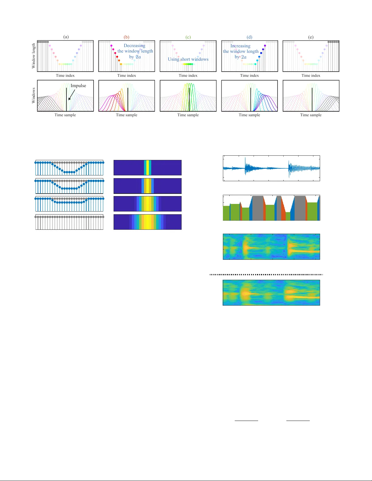
IEEE/A CM TRANSA CTIONS ON A UDIO, SPEECH, AND LANGU A GE PR OCESSING, V OL. XX, NO. X, XXXX 20XX 1 SELEBI: Percussion-a w are T ime Stretching via Selecti v e Magnitude Spectrogram Compression by Nonstationary Gabor T ransform Natsuki Akaishi, Student Member , IEEE , Nicki Holighaus, Member , IEEE , K ohei Y atabe, Member , IEEE Abstract —Phase vocoder -based time-stretching is a widely used technique f or the time-scale modification of audio signals. Howev er , con ventional implementations suffer from “percussion smearing, ” a well-known artifact that significantly degrades the quality of percussi ve components. W e attribute this artifact to a fundamental time-scale mismatch between the temporally smeared magnitude spectrogram and the localized, newly gen- erated phase. T o address this, we pr opose SELEBI, a signal- adaptive phase vocoder algorithm that significantly reduces percussion smearing while preser ving stability and the perfect reconstruction property . Unlike conventional methods that rely on heuristic processing or component separation, our approach leverages the nonstationary Gabor transf orm. By dynamically adapting analysis window lengths to assign short windows to intervals containing significant energy associated with per cussive components, we directly compute a temporally localized magni- tude spectr ogram fr om the time-domain signal. This approach ensures greater consistency between the temporal structur es of the magnitude and phase. Furthermore, the perfect reconstruc- tion property of the nonstationary Gabor transform guarantees stable, high-fidelity signal synthesis, in contrast to previous heuristic approaches. Experimental results demonstrate that the proposed method effectively mitigates percussion smearing and yields natural sound quality . Index T erms —Phase vocoder , time-frequency analysis, adapti ve analysis window , phase derivati ve, percussion smearing. I . I N T R O D U C T I O N T IME stretching, a process that modifies the time-scale of a signal without altering its pitch, is a fundamental tool in modern music production, with applications ranging from audio remixing to transcription [1], [2]. The ideal goal is to obtain a time-stretched signal that perfectly preserves the musical characteristics of the original, such as its timbre, clarity , and dynamics. T o achie ve high-quality results, a wide variety of time-stretching methods hav e been proposed [3], [4], [5], [6], [7], [8], [9], [10], [11], [12], [13], [14]. The phase vocoder (PV) [3], [4] is one of the most widely used techniques for time-stretching. This approach operates in the time-frequency (T -F) domain: It computes the short-time Fourier transform (STFT), generates a new phase appropriate Manuscript received XXXX XX, XXXX; revised XXXXX XX, XXXX; accepted XXXXX XX, XXXX. Date of publication XXXXX XX, XXXX; date of current version XXXXX XX, XXXX. The associate editor w as XXXXX XXXX. Natsuki Akaishi and Kohei Y atabe are with T okyo Uni versity of Agriculture and T echnology , T okyo 184-8588, Japan (e-mail: natsu61aka@gmail.com; yatabe@go.tuat.ac.jp). Nicki Holighaus is with Acoustics Research Institute, Austrian Academy of Sciences, W ohllebengasse 12–14, 1040 V ienna, Austria (nicki.holighaus@oeaw .ac.at) Phase vocoder process PV (with phase locking) Proposed method Original signal T- F representation Stretched signal DGT NSDGT Resynthesis Resynthesis Mismatch Leakage Less leakage Fig. 1. Block diagrams of the basic method, PV with identity phase locking [15] (left), and the proposed method (right). By leveraging NSDGT, the proposed method synthesizes the target signal from T -F representations in which both the magnitude and phase spectrograms of percussi ve components are highly concentrated in the time direction. for the modified time-scale, and resynthesizes the signal using the overlap-add (OLA) technique with an extended hop size. Although the PV is a well-established technique that has been continuously refined [5], [10], its fundamental logic builds on the sinusoidal signal model, i.e., it assumes that the signal is a sum of sinusoids. This model is effecti ve for tonal content because time-shifts are represented by a well-defined, predictable phase shift. Howe ver , it is ill-suited for percussiv e components, which cannot be represented by a sum of fe w sinusoids. Therefore, time-shifting of percussiv e components cannot be modeled as such a phase shift. As a result, the PV often introduces a well-kno wn artifact known as per cussion smearing . As illustrated in Fig. 1 (top-right), the stretched per - cussiv e components suffer significant de gradation, losing their original temporal characteristics due to undesired leakage. T o alle viate this, various “percussion-aware” methods have been proposed. Howe ver , they either rely on an a priori separation of the signal into tonal and percussiv e components for indi vidual processing [10], [11] (Class A), which in v ariably introduces artifacts due to imperfect separation, or the y suf fer , to various degrees, from magnitude-phase mismatch [9], [12], [13], [14] (Class B), inhibiting the elimination of percussion smearing. IEEE/A CM TRANSA CTIONS ON A UDIO, SPEECH, AND LANGUA GE PR OCESSING, V OL. XX, NO. X, XXXX 20XX 2 In this paper , we address the fundamental limitation of Class B methods 1 : the inconsistency between magnitude and phase. While these methods often succeed in preserving the phase relationships required for transients (i.e., vertical phase coherence), the corresponding magnitude spectrograms are inevitably smeared due to the time-stretching process. This results in percussi ve components being spread across a dilated time interval, which contradicts the localized phase informa- tion. W e posit that this mismatch is the primary cause of percussion smearing, as illustrated in Fig. 1 (left). T o address this, we propose computing spectrograms with improved tem- poral localization specifically where percussiv e components are present, thereby aligning the magnitude representation with the localized phase (Fig. 1, right). While our pre vious work [16] attempted to mitigate this issue through heuristic time-frequency bin shifting, the proposed method provides a theoretical foundation for ener gy preservation and stable synthesis. T o achiev e this magnitude squeezing in a mathemat- ically rigorous manner , this paper proposes a method named SELEBI ( SELE cti ve window compression with sta B le I n version). Our method le verages the Nonstationary Gabor T ransform (NSDGT) [17], a time-frequency representation framew ork that allows for adapti ve, non-uniform windo wing and sampling while retaining perfect reconstruction properties. W e exploit this flexibility by adaptiv ely assigning shorter windows to percussi ve regions, thereby directly obtaining a magnitude spectrogram with a desired temporal resolution. Crucially , the underlying mathematical frame work of the NSDGT guarantees that this adaptive processing results in a stable and high-fidelity synthesis. The rest of the paper is or ganized as follo ws. Section II revie ws the fundamentals of the NSDGT and PV -based time stretching. Section III discusses the core component of the proposed method: Sharply resolving percussiv e events to re- duce percussion smearing in time-stretched audio. Section IV presents the proposed SELEBI algorithm. Section V discusses the feasibility of a bounded-delay implementation for on- line applications. Section VI provides experimental results validating our method, and Section VI concludes this paper . I I . P R E L I M I N A R I E S A. Notation The sets of natural numbers, integers, real numbers, and complex numbers are denoted by N , Z , R , and C , respecti vely . Matrices are denoted by bold capital letters (e.g., A ), and their element at the i -th row and j -th column is denoted by A [ i, j ] . V ectors are denoted by bold lo wer -case letters (e.g., v ), and their i -th element is denoted by v [ i ] . For the purpose of this paper , we identify the cyclic group of order N , denoted by Z N , with the integers 0 , . . . , N − 1 . The following operations are always considered pointwise: ⊙ (multiplication) ⊘ (division), | · | (modulus / absolute value), and Arg ( · ) (complex argument). A sequence indexed by k ∈ K ⊂ N is denoted by {· k } k ∈ K . 1 Our approach does not rely on signal separation, thereby av oiding the artifacts associated with Class A methods. This allo ws us to focus solely on the limitations of Class B methods. (a) DGT (long win.) (b) DGT (short win.) (c) NSDGT 0.5 0.6 0.7 0.8 Time [sec] 0 1000 2000 3000 Frequency [Hz] 0.5 0.6 0.7 0.8 Time [sec] 0.5 0.6 0.7 0.8 Time [sec] Fig. 2. Comparison of windows and spectrograms for the DGT and NSDGT. The upper boxes illustrate the windo w shift in the time domain, where representativ e DGT windo ws are highlighted in black for clarity . The bottom boxes display the corresponding spectrograms for (a) DGT with a long window , (b) DGT with a short windo w , and (c) the NSDGT. The floor , ceiling, and nearest-integer (rounding) functions are denoted by ⌊·⌋ , ⌈·⌉ , and ⌊·⌉ , respecti vely . The Frobenius norm is denoted by ∥ · ∥ F . B. Discr ete Gabor T ransform (DGT) The DGT coefficients X ∈ C M × N of a signal x ∈ R L with a window function g ∈ R L are defined as [18] X [ m, n ] = L − 1 X l =0 x [ l ] g [ l − an ] e − i 2 π m ( l − na ) / M , (1) where i = √ − 1 , a ∈ N is the hop size, l ∈ Z L is the time index, n ∈ Z N is the time-frame inde x, m ∈ Z M is the frequenc y index. The signal length L is set to satisfy aN = bM = L , where b ∈ N is the frequency decimation parameter . The in verse DGT (iDGT) is gi ven by o verlap-adding the individual, synthesized time frames: b x [ l ] = N − 1 X n =0 e g [ l − na ] · M − 1 X m =0 X [ m, n ] e i 2 π ml/ M , (2) where e g is the synthesis windo w . When the (analysis) window g has no more that M (consecutiv e) nonzero samples, then by choosing e g [ l ] = g [ l ] M P N − 1 n =0 g [ l − na ] 2 , (3) we achie ve error -free reconstruction, i.e., x [ l ] = b x [ l ] , provided that the denominator in Eq. (3) is strictly positive. As commonly done in the acoustics literature, we refer to X as (complex) spectr ogram . Furthermore, M = | X | and Φ = Arg ( X ) are termed the magnitude and phase spectr ograms , respectiv ely [19]. IEEE/A CM TRANSA CTIONS ON A UDIO, SPEECH, AND LANGUA GE PR OCESSING, V OL. XX, NO. X, XXXX 20XX 3 C. Nonstationary DGT (NSDGT) The NSDGT [17], [20] generalizes the DGT by integrat- ing variable hop sizes, windo w functions and numbers of frequency channels per time-frame into a flexible, in vertible T -F representation. In this paper , howe ver , we only consider variation of hop sizes and windo w functions, while fixing the number of frequency channels. For the n -th time frame, let a n ∈ N be the hop size, g n ∈ R W n be the window function, W n ∈ N be the window length, and M ∈ N be the number of frequency channels. Further define by A 0 = 0 and A n = P n j =1 a n the time position of the n -th time frame. Hence, the NSDGT coefficients X NS ∈ C M × N as per [17] are giv en by X NS [ m, n ] = L − 1 X l =0 x [ l ] g n [ l − A n ] e − i 2 π m ( l − A n ) / M . (4) For X NS , | X NS | and Ar g ( X NS ) we adopt the terminology used for the DGT , i.e., we refer to them as (magnitude/phase) spectr ogram . Fig. 2 provides an example of a flexible T -F representation using the NSDGT. As sho wn in (a) and (b), the standard DGT exhibits a well-known trade-off: a long window achieves good frequency localization for sinusoidal components, while a short windo w provides good temporal localization for percus- siv e components. Most realistic signals, howe ver , contain both component types, often e ven simultaneously . In contrast, the NSDGT (c) employs adaptiv e windowing with long windows for sinusoidal regions, short windows for percussive regions [17], and intermediate lengths for mix ed components, resulting in improved time-frequency localization for the entire signal. D. PV -based T ime Stretc hing The PV begins by computing a DGT , see Eq. (1), with the analysis hop size a . Subsequently , the phase spectrogram is modified while leaving the magnitude spectrogram unchanged. Finally , a time-stretched signal is synthesized by applying an in verse DGT (iDGT) with the synthesis hop size e a gi ven by e a = ⌈ αa ⌉ . Here, α ∈ R + is the desired stretching factor 2 . This results in the final time-stretched signal b x ∈ R e aN . Restricting, for the sake of a more concise treatment, to the case of constant stretch factor α , the main difference between PV v ariants concern the specific modification applied to the phase spectrogram. In the classical phase vocoder [3], [4], the new phase spectrogram e Φ is computed by scaling the time-direction partial deri v ati ve ∆ t Φ of the phase Φ with α before inte grating the phase along time within each channel. Commonly , this process is performed in two steps: The deriv ati ve is approximated as (∆ t Φ)[ m, n ] = 1 a  Φ[ m, n ] − Φ[ m, n − 1] − 2 π ma M  2 π + 2 π m M , (5) 2 Percussion smearing is observed only when the time-scale is extended, such that we consider α > 1 here. where [ · ] 2 π = · − 2 π ⌊· / 2 π ⌉ is the principal argument calcu- lation. Subsequently , e Φ is computed with the recursi ve phase propagation formula [15], e Φ[ m, n ] = e Φ[ m, n − 1] + e a (∆ t Φ)[ m, n ] . (6) V arious heuristic modifications have been proposed to the estimation of ∆ t Φ or the integration step, in order to im- prov e perceptual quality [15], [21], some of which have been integrated in a prior extension of the PV using NSDGT [9]. Con ventional phase generation in PV -based time stretching typically relies solely on the time-direction phase deri vati ve to model phase e volution, as in Eq. (5) and (6). This approach essentially assumes a sinusoidal model, treating frequency channels independently . Consequently , it disregards the verti- cal phase relationships that are crucial for preserving transient sharpness, leading to percussion smearing [10]. T o mitigate this, it is common to apply phase-locking techniques [9], [15], [21], [22], which heuristically enforce consistency between adjacent channels to maintain vertical coherence. Moving be yond heuristics, the method proposed in [8] intro- duces a more rigorous frame work by adapting Phase Gradient Heap Inte gration [23], a technique originally de veloped for phaseless reconstruction. Unlike standard PV or simple phase- locking, this approach considers the full phase gradient; that is, it estimates and scales both the time-direction deri vati ve ∆ t Φ and the frequency-direction deriv ativ e ∆ f Φ . By per - forming adaptiv e numerical integration along the optimal path in the time-frequency plane, this method achieves significant improv ements in perceptual quality and reduces percussion smearing without relying on potentially unreliable heuristics. Howe ver , ev en with advanced phase generation techniques like [8] or other percussion-aware phase refinements [9], [12], [13], [14], artif acts remain unavoidable, especially at large stretching factors α . This is due to a fundamental mismatch between the estimated phase and the magnitude spectrogram. While these methods striv e to reconstruct a temporally lo- calized phase corresponding to a transient, the underlying magnitude spectrogram M remains temporally smeared due to the stretching process. This inconsistency between the lo- calized phase and the spread magnitude pre vents the complete elimination of percussion smearing. I I I . R E D U C I N G P H A S E - M A G N I T U D E M I S M AT C H T H RO U G H I M P ROV E D T R A N S I E N T C O N C E N T R A T I O N Our proposed method is based on the hypothesis that, be- sides imperfect phase estimates, the primary cause of percus- sion smearing is a time-scale mismatch between the magnitude M and the estimated phase e Φ used to synthesize the time- stretched signal. Successful improvements to the PV , such as [13], [8], use the magnitude as a cue to generate a localized phase, implicitly or even explicitly enforcing a stretch factor of 1 for percussi ve ev ents. Ho we ver , the unchanged magnitude spectrogram, when interpreted using the synthesis hop size e a , indicates temporal smearing of said ev ents, leading to arti- ficial lengthening during synthesis, which cannot be entirely suppressed by a better phase estimate. T o overcome this, our key idea is to construct a magnitude spectrogram that sharply IEEE/A CM TRANSA CTIONS ON A UDIO, SPEECH, AND LANGUA GE PR OCESSING, V OL. XX, NO. X, XXXX 20XX 4 represents percussiv e ev ents. W e employ a dual strategy: (1) shortening the analysis windo w to enhance temporal resolu- tion, and (2) reducing the number of time-frames cov ering the ev ent to minimize inter-frame smearing. By allo wing these tw o mechanisms to work in tandem, we aim to keep the transient representation sharp, ef fecti vely preserving its original time- scale, while allo wing the tonal resonances to be stretched naturally . Fig. 3 illustrates the effect of this magnitude “squeezing”. In the standard PV approach (Fig. 3(a)), the use of a fixed, long analysis windo w with high o verlap distrib utes the per- cussiv e energy across a broad sequence of time frames. When stretched, this sequence expands, ine vitably causing the synthesized transient to be less sharp and introducing phase- magnitude mismatch (purple regions). In contrast, our method (Fig. 3(b)) dynamically adapts the representation. By simulta- neously shortening the window length ( ⋆ 1 ) and reducing the frame density ( ⋆ 2 ) in the vicinity of the transient, the method effecti vely “squeezes” the signal energy into a narro wer re gion on the stretched grid. This concentration ensures that the transient is synthesized with a sharpness comparable to the original signal, drastically reducing leakage and smearing. In our pre vious conference paper [16], we presented a preliminary , heuristic method designed to achie ve a similar effect. In that method, we shift T -F bins horizontally toward the center of the corresponding percussi ve e vent. F or compatibility with the used DGT and existing phase estimation schemes for time-stretching, e.g., Eq. (6), the resulting, non-uniform spectrogram is resampled on a uniform temporal grid after spline interpolation. Although this approach provides an ac- ceptable improvement in percussive sound quality , its heuristic design introduces se veral potential issues: 1) The bin-shifting operation is not ener gy-preserving; temporally localizing the bins without properly concentrating their energy led to a slight reduction in v olume. 2) Spline interpolation of the spectrogram neglects the effects of original choice of analysis window and hop size, introducing approximation errors. I V . P RO P O S E D M E T H O D : S E L E B I In this section, we introduce SELEBI, the proposed time- stretching method designed to suppress percussion smearing. As discussed in the previous section, this is achiev ed by designing a T -F representation that enforces temporal concen- tration of transients. T o this end, we emplo y the NSDGT, locally adapting both the window lengths W n , as seen in Fig. 3(b), and hop sizes a n , in a small neighborhood of detected percussive ev ents. The ef ficacy of this approach is demonstrated in Fig. 3. While a standard DGT magnitude spectrogram temporally smears an impulse (second ro w , left), our NSDGT-based spectrogram maintains sharp localization (second row , right). Crucially , the NSDGT framework resolves the limitations of our previous method [16]: Unlike the simple bin-shifting which resulted in energy loss, the NSDGT is mathematically rigorous and inv ertible, thereby guaranteeing energy preserv a- tion. Furthermore, in contrast to the interpolated spectrogram in [16], the NSDGT structure retains well-defined windo w and hop parameters, leading to a better phase estimate. (a) Basic method Percussive component Other components (b) Transient concentration Squeezing Generated phase Magnitude Stretched signal Mismatched part Signal & wins. Less or no leakage Undesired leakage ★ 1 ★ 2 Time frames covering the percussive components Fig. 3. Conceptual illustration of time-directional spectrogram “squeez- ing. ” (a) The conv entional PV -based method using DGT . (b) The proposed method utilizing transient concentration. The top row displays the input time- domain signal (amplitude vs. time) and the analysis window functions. The second and third rows schematically represent the magnitude spectrogram and the corresponding generated phase, respectiv ely . The bottom row sho ws the synthesized time-stretched signal. In these schematic representations, the percussive component is colored red, and the windo ws capturing this component are emphasized (non-percussive components are omitted in this row for clarity). In the spectrograms, the red area highlights the percussiv e component, while the blue and green areas represent the magnitude and phase of the other components, respecti vely . Because the percussive interv al is maintained at its original time-scale, it appears compressed relati ve to the new , stretched time axis (illustrated below the spectrograms). The bottom panel details the synthesis of the percussi ve component across the new time frames. The markers ⋆ 1 and ⋆ 2 highlight the key innovations of the proposed method: shortening the windo w length and reducing the number of time frames, respecti vely . A. Flow of SELEBI The flow of SELEBI is summarized in Alg. 1 and illustrated in Fig. 4. Our method first performs a preprocessing stage (lines 1–3) to determine the NSDGT parameters, including window lengths and hop sizes. T o appropriately modify the windows, the algorithm first identifies the position of percus- siv e components (line 1, Alg. 2), using onset detection based on harmonic-percussiv e sound separation (HPSS) [24]. It then calculates a corresponding compression rate , defined as the proportion of frequency bins in that frame that are classified as percussive. The compression rate determines the shortest window length, used at the onset position. This procedure ensures that strong transient e vents remain highly concentrated and reduces the presence of audible artifacts when transient and harmonic ev ents overlap. A preliminary (constant) analysis hop size is set based on the selected time-scale factor , such that, under the assumption that the longest admissible windo w length be used e verywhere, sufficient overlap remains after time-stretching. At each time position, a desired window length is determined based on the detected onsets and compression rates (line 2, Alg. 3). In regions where the windo w length is reduced, the original hop IEEE/A CM TRANSA CTIONS ON A UDIO, SPEECH, AND LANGUA GE PR OCESSING, V OL. XX, NO. X, XXXX 20XX 5 Algorithm 1 Proposed method (SELEBI) Input: x ∈ R L Output: b x ∈ R αL 1: paramsForW inLen = computCompRate ( x ) ▷ Sec. IV -B, Alg. 2 2: winLen = computW inLen ( paramsForW inLen ) ▷ Sec. IV -C, Alg. 3 3: [ winLen , hopSize ] = modifyHopSize ( winLen ) ▷ Sec. IV -D 4: X NS = NSDGT ( x , winLen , hopSize ) ▷ Eq. (4) in Sec. II-C 5: Φ = genPhase ( X NS , hopSize ) ▷ Sec. IV -E 6: b x = synthesis ( X NS , Φ , hopSize ) ▷ Sec. II-D Sec. IV -C, Alg. 2 Sec. IV -B, Alg. 3 Sec. IV -D Sec. IV -E Sec. II-D Original signal Onset detection and compression rate calculation W indow length calculation Hop size modification NSDGT Phase generation Synthesis based on inverse NSDGT Stretched signal Fig. 4. The flow of the proposed method. The left column details the NSDGT parameter calculation, while the right column illustrates the subsequent processing steps. size is too large and would lead to insufficient coverage, such that ne w , narro wer time positions are adaptiv ely chosen for appropriate coverage, while ensuring that the number of time frames covering the percussi ve ev ent remains small (line 3, Alg. 3). Using these parameters, the NSDGT is computed to obtain a “squeezed” magnitude spectrogram (line 4). Subse- quently , a modified phase generation procedure, adapted to be compatible with v ariable hop sizes, is applied (line 5), and the time-stretched signal is synthesized using the inv erse NSDGT (line 6). The following subsections detail each part of this process: parameter calculation (Sec. IV -B), selecti ve window compres- sion (Sec. IV -C), hop size determination (Sec. IV -D), and modified phase generation (Sec. IV -E). Although the proposed method uses an adaptiv e hop size, the figures in Sec. IV -B and Sec. IV -C show a fixed hop size for simplicity . B. Onset Detection and Compr ession Rate Calculation In order to determine the adaptive window lengths used in SELEBI, it is necessary to identify the positions of percussi ve components and determine the corresponding compression rates. The windo w length compression itself is described in Sec. IV -C. Our method is deri ved from the spectral flux and weighted phase deviation onset detectors described in [25]. W e combine these methods and extend them to quantify the relativ e intensity of percussiv e components at the detected onsets. As such, determining the SELEBI parameters in volv es computing the DGT of the original signal, classifying T -F bins as percussi ve or not, and finally quantifying the proportion of percussiv e content within each onset frame. Fig. 5 illustrates the principles applied for onset detection and compression rate selection by ways of an example. The magnitude ratio (red line in panel (e)) is computed for each time frame by dividing the sum of percussive T -F bins across Algorithm 2 Computation of the compression rate Input: x ∈ R L Output: { r k } k ∈{ 1 ,...,K } , { I k } k ∈{ 1 ,...,K } 1: X = DGT ( x ) ▷ compute the spectrogram 2: Φ m = ∂ 2 Arg ( X ) /∂ τ ∂ ω ▷ compute the MPD of phase 3: M = M ( X , Φ m ) 4: ▷ compute the mask for separating percussive components 5: X p = X ⊙ M ▷ compute the masked spectrogram 6: r = filtering ( P M − 1 m =0 | X p [ m, n ] | ⊘ P M − 1 m =0 | X [ m, n ] | ) 7: ▷ compute the ratio of the percussive components in each frame 8:  { r k } k ∈{ 1 ,...,K } , { I k } k ∈{ 1 ,...,K }  = findPeaks ( r ) 9: ▷ find the positions of the pulse and decide their compression rates Algorithm 3 Computation of the window length vector Input: { r k } k ∈{ 1 ,...,K } , { I k } k ∈{ 1 ,...,K } , N half = ⌈ V / (2 a ) ⌉ Output: v ∈ N N 1: for k = 1 , . . . , K do ▷ for all percussi ve components 2: S k = ⌊ V − r 2 k (1 − 1 /α ) V ⌋ 3: ▷ calculate the smallest windo w length 4: for n = 1 , . . . , N do ▷ for all time indices 5: if | n − I k | ≤ N half then ▷ within the percussiv e interv als 6: V [ k , n ] = max ( S k , 2 a | n − I k | + V − 2 aN half ) 7: ▷ shorten the window length 8: else 9: V [ k , n ] = V ▷ retain the length 10: end if 11: end f or 12: end for 13: v = min ( V [1 , :] , . . . , V [ K, :]) ▷ select shorter lengths frequencies by the total magnitude summed across frequencies (dotted line). The final parameters are then extracted by detecting the peaks of this ratio (panel (f)) 3 , where the height and position of each peak correspond to the compression ratio r k and center position I k of a pulse. Alg. 2 details this procedure. Note that local fluctuations in the magnitude ratios are suppressed by applying a one-dimensional median filter (line 6, Alg. 2). W e now proceed to discuss the onset detection algorithm and the function M used to classify T -F bins as percussiv e, resulting in a binary mask M . T o compute M , we utilize the mixed-partial deriv ative (MPD) of the phase, MPD ( ω , τ ) = ( ∂ 2 Arg ( Y ) /∂ τ ∂ ω )( ω, τ ) as in [26], whereas a threshold on the magnitude | X | is additionally used to ignore T -F re gions with negligible energy , in which the phase is unstable. Fundamentally , an onset de- tection function based solely on | X | such as ( ∂ | X | /∂ τ )( ω , τ ) could be used, we found that magnitude information alone is often insufficient for reliable onset detection in complex, real-world signals containing div erse components. In these settings, we obtained improv ed identification accuracy with MPD. For details on the suitability of MPD for classification of predominantly percussiv e T -F bins, see [26] and [27], which argue that MPD ( ω , τ ) ≈ 0 at T -F bins containing purely sinusoidal components and MPD ( ω , τ ) ≈ 1 (possibly after scaling), at T -F bins containing only impulsive components, or ∂ 2 ∂ τ ∂ ω Arg ( Y )( ω , τ ) ≈  0 (if Y ( ω , τ ) is sinusoidal) , 1 (if Y ( ω , τ ) is impulsi ve) . (7) Using these properties of MPD, we can create a binary mask that remov es T -F bins that are not classified as percussi ve. For 3 For the detection of peaks of the ratio, we use the MA TLAB function findpeaks with “ MinPeakProminence ” = 0 . 1 . IEEE/A CM TRANSA CTIONS ON A UDIO, SPEECH, AND LANGUA GE PR OCESSING, V OL. XX, NO. X, XXXX 20XX 6                Fig. 5. Example of the computation of the compression rate. From top left to bottom right, (a) the magnitude spectrogram | X | , (b) the enhancement mask, (c) the enhanced spectrogram | X p | , (d) the frequency-directional sum of | X | , (e) the frequency-directional sum of | X p | , and (f) the compression rate r (the detected peaks are plotted in yellow). The mask in (b) is colored in white where M ( X , Φ mix )[ m, n ] = 1 . this paper , we consider the operator M : ( C M × N , R M × N ) → { 0 , 1 } M × N for generating said mask, defined by M ( X , Φ mix ) = M mag ( X ) ⊙ M p ( Φ mix ) , (8) where Φ mix ∈ R M × N is MPD corresponding to X , M mag ( X )[ m, n ] =  1 if | X [ m, n ] | > θ mag , 0 otherwise , M p ( Φ mix )[ m, n ] =  1 if θ p < Φ mix [ m, n ] − 1 < θ p , 0 otherwise , (9) and θ mag , θ p , θ p > 0 are hyperparameters used for thresh- olding. The two masks serve distinct purposes: M mag elim- inates low-magnitude (noisy) components, and M p enhances percussiv e components. Fig. 5(b) shows the resulting mask M = M ( X , Φ m ) . This mask successfully reveals even subtle percussiv e components (highlighted in white), which leads to the effecti ve enhancement of these components, as shown in (c). C. Selective W indow Length Compr ession Once the center position I k , and the compression ratio r k ∈ [0 , 1] of percussi ve e vents has been determined, SELEBI adjusts the length of the analysis windows used in the neigh- borhood of I k , such that temporal smearing is minimized. The adaptation process is illustrated in Fig. 6. It ensures that the impulse is “observed” only by few , short windows, rather than being captured by many long windows that produce smearing after time-stretching. The length of the windows used is determined by the compression rate r k , with lar ger r k enforcing shorter windows of length S k at and around the center of the k -th percussive ev ent, as sho wn in Fig. 7. The length S k is determined by the formula: S k = ⌊ V − r 2 k (1 − 1 /α ) V ⌋ , (10) where V is the length of the original, long analysis window , and α > 0 is the stretching factor . Note that the window length remains unchanged when r k = 0 , as shown in the bottom row of Fig. 7. T o ensure a stable representation of the signal surrounding the percussive e vent, SELEBI gradually varies the window length from the full length V to the target length S k (and vice versa) by successively adjusting the lengths by multiples of the hop size (e.g., 2 a ), as sho wn in Fig. 6, panels (b) and (d). W e now summarize the procedure of calculating the window length for each time frame, see Alg. 3 for a formal description. W e be gin by looking at each percussiv e event individually . Let N half = ⌈ V / (2 a ) ⌉ denote the number of frames between the edge of the (long) analysis window and its center . This number determines the time indices left and right of I k that will be assigned an adapted window length. Starting from time index J k, − = I k − N half , the window length is shortened by 2 a , until a length of S k is reached, i.e., at index J k, − + j , we assign window length max { V − 2 a ( j − 1) , S k } , for 0 ≤ j ≤ N half + 1 . Like wise, with J k, + = I k + N half , we assign windo w length max { V − 2 a ( j − 1) , S k } to index index J k, + − j , for 0 ≤ j ≤ N half + 1 . This ensures that the center of the percussive ev ent is cov ered by no more than 2 ⌈ S k / (2 a ) ⌉ + 1 windows of length S k and all other analysis time frames do not contain said center . This process is illustrated in Fig. 6. In the case that the intervals [ J k, − , J k, + ] overlap, for different values of k , we select the minimum of all assigned window lengths. This can be seen in the example shown in Fig. 8. D. Modification of Hop Sizes In practice, using varying windo w sizes at equidistant time positions na is either computationally wasteful (small hop size a ) or leads to synthesis instability where short windows are used (large hop size a ). Whereas the former has negati ve impact on the algorithm’ s demands in terms of computation time and hardware, the latter may produce synthesis artifacts and lead to poor quality audio output. T o resolve this, we construct a variable hop size NSDGT by choosing hop sizes adapted to the windo w length determined in Sec. IV -C. Specif- ically , we emplo y a standard analysis hop size, a , for non- percussiv e regions (long windows) and an adaptiv e hop size, b a k , for percussive regions (short windows). In the transition regions, we smoothly v ary the hop sizes and window lengths via interpolation to prevent sampling artifacts. T o maintain sufficient overlap in the percussiv e regions, b a k is deri ved from the short window length S k and the time-stretching factor α , which will be defined later . W e describe the hop size determination process. First, the time frames are segmented into four distinct region types based on the target window length configuration: (i) constant (long), (ii) constant (short), (iii) transition (long to short), and (i v) transition (short to long). The time positions and window lengths at the boundaries of these regions are fixed to the original grid. For type (i) regions, the original grid remains unaltered. In type (ii) regions, we introduce an adaptiv e hop size defined as b a k = ⌊ S k / ( αβ ) ⌉ , where β > 1 is a parameter controlling the overlap ratio (empirically set to β = 4 ). T o fill the fixed region duration N org a , where N org is the number of frames in the original grid, we assign the hop size b a k IEEE/A CM TRANSA CTIONS ON A UDIO, SPEECH, AND LANGUA GE PR OCESSING, V OL. XX, NO. X, XXXX 20XX 7                                                  Using short windows Decreasing the window length by Increasing the window length by Impulse (a) (b) (c) (d) (e) Fig. 6. Concept of the window length adjustment in the proposed method. The top row shows the target window length, while the bottom ro w shows the corresponding analysis windows. The colors in the top row match those in the bottom row . Stages (a)–(e) illustrate the window behavior as it encounters an impulse. r = 1 : 0 Window length NSDGT r = 0 : 8 r = 0 : 4 r = 0 Fig. 7. Effect of compression rate r on window length (left) and the resulting impulse magnitude spectrogram (right). The left panels plot the window lengths (vertical axis) v ersus time (horizontal axis), where the original windo w length is shown in gray , and the modified window length is shown in blue. The right panels show the corresponding magnitude spectrograms (frequency vs. time) of an impulse, obtained using the window functions from the left. From top to bottom, the ro ws show compression rates of r = 1 . 0 , 0 . 8 , 0 . 4 , and 0 , chosen for visibility . sequentially from the beginning of the region. The final hop size serves as a compensation frame to absorb the residual time dif ference 4 , calculated as aN org − b a k ⌊ aN org / b a k ⌋ . In cases where two percussi ve e vents occur in close proximity , type (ii) regions may become adjacent; in such instances, the window length and hop size change stepwise between these regions. For transition regions (types (iii) and (iv)), the hop size is v aried linearly to smoothly connect the adjacent re gions. T o determine the linear trajectory , the starting and ending hop sizes, denoted as a st and a end , must first be defined based on the transition pattern summarized in T able I. Patterns (A) and (B) simply utilize the standard hop size a and the adaptiv e hop size b a k . Conv ersely , patterns (C) and (D) represent cases where the window length trajectory switches direction (i.e., it expands and immediately transitions to shrinking) without returning to the long windo w state (type (i)), as seen around the 350-th sample in Fig. 8. In such cases, we define an intermediate hop size based on the boundary window length V bnd as ˘ a k = ⌊ a V bnd /V ⌉ . According to the window length formulation in Sec. IV -C, V bnd between the k -th and ( k + 1) -th percussi ve 4 If the duration is divisible by b a k without remainder, this residual is zero.                                !"#$%& Fig. 8. Example of adaptive window length adjustment and the resulting NSDGT spectrogram for a bongo signal. The panels display , from top to bottom: the original wa veform, the adapti ve windo w length at each time index, the resulting NSDGT spectrogram, and the standard DGT spectrogram. For clarity , the middle panel is color-coded to correspond with the adjustment stages shown in Fig. 6: non-percussive regions (gray; (a), (e)), pre-pulse (red; (b)), pulse center (green; (c)), and post-pulse (blue; (d)). components is determined as V bnd = a ( I k +1 − I k ) + V − 2 aN half . W e state the procedure focusing on type (iii) transitions. T o maintain the total duration of the region, N org a , while linearly varying the hop size, we first calculate the target number of new frames, N new , as N new =  2 a st + a end  aN org − a st − a end 2  . (11) T o av oid generating unnaturally small compensation hop sizes in regions where lar ger hop sizes are intended, we arrange the hop positions starting from the boundary with the larger IEEE/A CM TRANSA CTIONS ON A UDIO, SPEECH, AND LANGUA GE PR OCESSING, V OL. XX, NO. X, XXXX 20XX 8 T ABLE I H O P S I Z E D E FI N I T I O N S F O R E A C H T R A N S I T I O N T Y P E . T ype of transitions Hop size settings Before T ransition After a st a end (A) (i) (iii) (ii) a b a k (B) (ii) (iv) (i) b a k a (C) (ii) (iv) (iii) b a k ˘ a k (D) (iv) (iii) (ii) ˘ a k b a k (E) (ii) (iii) , (i v) (ii) b a k b a k +1 window length. Consequently , the hop size a l at the l -th frame from this starting point is defined as a l =  a max − l N new ( a max − a min )  , (12) where a max and a min denote the larger and smaller values between a st and a end , respectiv ely . This formulation is deri ved by solving P N new l =1 a l = N org a under an integer constraint. Any residual time difference due to rounding is compensated for by inserting a correction hop size of ⌊ ( N org a − P N new l =1 a l ) / 2 ⌋ at the end of the sequence (i.e., near the short windows). T ype (iv) transitions are treated analogously , starting from the endpoint corresponding to the larger windo w length (i.e., the end of the region). Once the hop sizes are determined, the window lengths for the ne w grid are deri ved via linear interpolation based on the correspondence with the original grid. An example of the hop size modification is illustrated in Fig. 9. The timeline is categorized into three types of regions based on window length behavior: decreasing (red), constant (green), and increasing (blue). The constant regions correspond to either the non-percussiv e state (using a ) or the percussive state (using b a ). In the transition regions, the hop size varies linearly . This strategy effecti vely handles adjacent percussive ev ents, as shown in Fig. 9 (right): the hop size widens after the first pulse (approx. 2500–2800-th sample) before narro wing again for the second. This adaptive sampling ensures that the “window compression” described in Sec. IV -C, intended to limit transient observation, is successfully achieved. E. Modification of Phase Generation V ariants of the PV , see Sec. II-D, usually employ phase generation methods tailored to a uniform hop size. Howe ver , it is straightforward to adapt formulas Eq. (5) and Eq. (6), so long as the number of frequency bins is equal to a constant M for all time frames, as considered here. Simply exchange a for a n in Eq. (5) and ˜ a for ⌈ αa n ⌉ in Eq. (6). Other standard techniques, such as identity phase locking, remain directly applicable. In principle, it is possible to v ary the number of frequency bins M at each time step as well, e.g., proportional to the window length to further reduce oversampling. Ho w- ev er, doing so would require both the use of directional deriv ativ es and oblique integration paths, introducing signif- icant computational (and book-keeping) overhead, as well as implementation complexity . Furthermore, the quality of PV - based time-stretching benefit from a high number of frequency channels (i.e., high oversampling) in our experience. Overall, (a) (b) 1000 2000 3000 4000 Time sample (c) 1000 2000 3000 4000 Time sample Fig. 9. Example of smooth hop size adjustment and impulse observation (corresponding to Sec. IV -D). The left column sho ws a single impulse, while the right column sho ws two adjacent impulses of differing amplitudes. Note that the small impulse on the right is embedded in Gaussian noise to simulate a less-percussive sound. (a) plots the adaptive window length (stems) at each hop position, with gray line indicating the positions of a large, fixed hop size; (b) illustrates the corresponding shifting windows; and (c) shows the observed amplitude, with the DGT -based magnitude in gray for comparison. The windo w coloring scheme is the same as in Fig. 8. Current time position Look-ahead frames T ar get Onset detection and compression rate calc. Following procedures Setting windows and hop sizes, NSDGT , phase generation, inverse NSDGT Detected peak Pre-analysis Fig. 10. Conceptual diagram of a bounded-delay , online implementation. The left panel illustrates the pre-analysis of a target percussiv e component (red) using the DGT . The left edge represents the current time position, and the analysis windows corresponding to the required look-ahead frames are highlighted in blue. The top-right panel depicts the onset detection and compression rate calculation (corresponding to Fig. 5 (f)), displaying the magnitude ratio in gray and the detected peak in yellow . The bottom-right panel outlines the subsequent procedures. the (moderate) reduction in ov ersampling may be outweighed by the loss in audio quality and increased comple xity of the implementation. V . C O N S I D E R A T I O N S F O R B O U N D E D - D E L AY , O N L I N E I M P L E M E N T A T I O N Although the present paper and the associated implementa- tion of SELEBI focus on of fline processing, we briefly discuss the requirements for a bounded-delay , online implementa- tion. As illustrated in Fig. 10, the primary factor determining the feasibility of such an implementation is the look-ahead required by the pre-analysis stage for onset detection and compression rate estimation (Sec. IV -B). Accurately capturing these percussi ve components requires a sufficient observ ation buf fer . The left panel of Fig. 10 depicts this pre-analysis stage using a standard DGT . T o provide the necessary conte xt for identifying local maxima as the amplitude ev olves (top-right panel), this buf fer needs to span approximately twice the maximum analysis window length of the adapted NSDGT, as can be seen in the left panel. Once the peak is detected IEEE/A CM TRANSA CTIONS ON A UDIO, SPEECH, AND LANGUA GE PR OCESSING, V OL. XX, NO. X, XXXX 20XX 9 T ABLE II C O M PAR I S O N O F E R RO R M E A S U R E M E N T S F O R S Y N T H E T I C S I G N A L S ( S E C . V I - A ) . T H E TO P A N D B OT T O M R O W S S H OW T H E R E S U LT S O F 2 × A N D 4 × S T R E T C H I N G , R E S P E C T I V E LY . “ D I A L G A ( P V D R ) ” D E N O T E S D I A L G A W I T H P V D R P H A S E G E N E R ATI O N , A N D S I M I L A R LY F O R OT H E R M E T H O D S . T H E B E S T A N D S E C O N D - B E S T S C O R E S A R E I N B O L D W I T H B L U E A N D L I G H T B L U E B AC K G RO U N D S , R E S P E C T I V E LY . PV PVDR PVHP DIALGA DIALGA SELEBI SELEBI (PV) (PVDR) (PV) (PVDR) α = 2 Impulse 0.2357 0.2402 0.6993 0.1009 0.1110 0.2326 0.2326 Sinusoid + Impulse 0.0113 0.0091 0.0130 0.0090 0.0092 0.0106 0.0051 Harmonic Sinusoid + Impulse 0.0129 0.0107 0.0139 0.0136 0.0107 0.0128 0.0098 T ransient 0.5806 0.5666 0.5924 0.5659 0.5647 0.5791 0.5552 Sinusoid + Transient 0.2506 0.2446 0.4244 0.2455 0.2445 0.2521 0.2414 α = 4 Impulse 0.3080 0.3080 1.3679 0.0559 0.0559 0.3069 0.3069 Sinusoid + Impulse 0.0220 0.0149 0.0242 0.0267 0.0168 0.0206 0.0151 Harmonic Sinusoid + Impulse 0.0298 0.0264 0.0307 0.0315 0.0270 0.0334 0.0265 T ransient 1.3835 1.3153 1.3838 1.4153 1.3097 1.3812 1.2266 Sinusoid + Transient 0.4746 0.4468 0.6175 0.4585 0.4407 0.4719 0.4316 and the compression rate is calculated, the subsequent steps, including adaptive windowing, phase generation, and the in- verse NSDGT, can be seamlessly e xecuted on the b uf fered frames. Consequently , the total algorithmic latency is primarily bounded by twice the maximum analysis window length. While this estimation assumes a conservati ve buf fer size, future improvements in peak detection, such as exploiting causal temporal features, could potentially reduce this look- ahead requirement, further minimizing the system delay . V I . E X P E R I M E N T S In this section, we ev aluate the quality of audio signals processed with SELEBI by comparing it with sev eral reference methods. The ev aluation uses both synthetic and real-world audio signals. For synthetic signals, we employ objectiv e metrics to compare the time-stretched results against a ground truth, whereas for real-world signals, we conduct subjecti ve listening tests. Audio demos are av ailable in our demo page 5 . The sampling frequency for all signals used in the experi- ments was 22 050 Hz 6 . The DGT used for the PV implementa- tion utilized a Hann windo w with a length of L = 2 11 samples (93 ms) and a synthesis hop size of 2 7 samples (5.8 ms). The number of frequency channels M was set to Lα (i.e., 2 11 α ), a configuration recommended for better synthesis quality . In accordance with the DGT settings, the longest window length in the NSDGT of the proposed method was set to V = 2 11 . The masking threshold parameters of the proposed method were set to θ mag = 0 . 01 , θ p = 0 . 5 , and θ p = 0 . 75 , based on informal pre-tests. A. Experiment A: Synthetic Signals W e use idealized, synthetic signals comprised of distinct characteristic combinations of pulses and sinusoids, to study fundamental patterns in and dif ferences between the proposed and reference methods. These signals were designed such that an ideal “ground truth” is a vailable for objecti ve e valuation. In ev ery case and configuration, we applied time-stretching and 5 https://natsukiakaishi.github .io/selebi/ 6 Corresponding to the native sampling rate of the dataset of real world recordings considered in Experiment B. ev aluated the synthesis accurac y based on the relative RMS difference of magnitude spectrograms, i.e., in the T -F domain. 1) T est Signals: W e performed time-stretching on five char - acteristic synthetic signals using relati ve amplitudes defined with respect to the transient peak. The fiv e signals were: (1) a unit impulse; (2) a mixture of an impulse and a 1000 Hz sinusoid scaled by a factor of 0 . 5 ; (3) a mixture of an impulse and harmonic sinusoids at 1000 , 2000 , and 3000 Hz with amplitudes scaled by 0 . 5 , 0 . 25 , and 0 . 125 , respectiv ely; (4) an exponentially decaying transient (based on a 50 Hz sinusoid); and (5) the same transient combined with a 1000 Hz sinusoid with half the peak amplitude of the transient. T o define the ground truth for the transient preservation quality , the ideal time-stretched signals were constructed by placing the transient components at the new time positions while maintaining their original durations and decay en velopes (i.e., without time-stretching the transients themselves). 2) Experimental Conditions: For this experiment, we con- sidered time-stretching by factors of 2 and 4. For each condition, we compared the following methods: classical PV with identity phase locking 7 [15] as a baseline, PVDR [8] as a percussion-agnostic state-of-the-art method, HPSS-based time stretching (PVHP) [10] as a standard percussi ve-a ware method, our previous method (DIALGA) [16], and the pro- posed method (SELEBI). For both DIALGA and SELEBI, we ev aluated versions using both classical PV and PVDR for phase generation. All methods, with the exception of PVHP , were implemented in MA TLAB using the L TF A T toolbox [28]; for PVHP , we used the authors’ original code [29]. 3) Evaluation: For the ev aluation, we use the following spectral error , calculated from the DGT coefficients of the ground truth signal ( X perf ) and the stretched signal ( X ): E ( X perf , X ) = ∥| X perf | − | X |∥ F ∥| X perf |∥ F . (13) The DGT coefficients for ev aluation utilized the same window settings ( W and e a ) as the synthesis process. T o mitigate boundary artifacts (due to signal truncation and circularity), 7 For impulse-only samples, the absence of sinusoidal components means that applying identity phase locking is equiv alent to not applying it. IEEE/A CM TRANSA CTIONS ON A UDIO, SPEECH, AND LANGUA GE PR OCESSING, V OL. XX, NO. X, XXXX 20XX 10 1.9 2 2.1 0 0.2 0.4 0.6 Ground truth 1.9 2 2.1 0 0.2 0.4 0.6 PV 1.9 2 2.1 0 0.2 0.4 0.6 PVDR 1.9 2 2.1 0 0.2 0.4 0.6 PVHP 1.9 2 2.1 0 0.2 0.4 0.6 DIALGA (PV) 1.9 2 2.1 0 0.2 0.4 0.6 DIALGA (PVDR) 1.9 2 2.1 0 0.2 0.4 0.6 SELEBI (PV) 1.9 2 2.1 0 0.2 0.4 0.6 SELEBI (PVDR) 1.9 2.1 0 200 400 600 800 Frequency [Hz] 1.9 2.1 0 200 400 600 800 1.9 2.1 0 200 400 600 800 1.9 2.1 0 200 400 600 800 1.9 2.1 0 200 400 600 800 1.9 2.1 0 200 400 600 800 1.9 2.1 0 200 400 600 800 [dB] 1.9 2.1 0 200 400 600 800 -50 0 50 Fig. 11. An impulse stretched 4 × . The leftmost column shows the ground truth (blue), while the remaining columns display the stretched signal for each comparison method (red). The figure is divided into two rows: the top row shows a magnified vie w of the impulse, and the bottom ro w displays the relative error spectrogram (log scale). In the top ro w , for visual clarity , the ground truth is plotted as a gray dashed line. In the error spectrogram (bottom), brighter colors indicate larger errors. 0 2 4 -0.5 0 0.5 Ground truth 0 2 4 -0.5 0 0.5 PV 0 2 4 -0.5 0 0.5 PVDR 0 2 4 -0.5 0 0.5 PVHP 0 2 4 -0.5 0 0.5 DIALGA (PV) 0 2 4 -0.5 0 0.5 DIALGA (PVDR) 0 2 4 -0.5 0 0.5 SELEBI (PV) 0 2 4 -0.5 0 0.5 SELEBI (PVDR) 0.6 0.8 -0.5 0 0.5 0.6 0.8 -0.5 0 0.5 0.6 0.8 -0.5 0 0.5 0.6 0.8 -0.5 0 0.5 0.6 0.8 -0.5 0 0.5 0.6 0.8 -0.5 0 0.5 0.6 0.8 -0.5 0 0.5 0.6 0.8 -0.5 0 0.5 0.6 0.8 0 200 400 600 800 Frequency [Hz] 0.6 0.8 0 200 400 600 800 0.6 0.8 0 200 400 600 800 0.6 0.8 0 200 400 600 800 0.6 0.8 0 200 400 600 800 0.6 0.8 0 200 400 600 800 0.6 0.8 0 200 400 600 800 [dB] 0.6 0.8 0 200 400 600 800 0 20 40 60 80 Fig. 12. Example of a transient signal stretched 4 × . The leftmost column shows the ground truth (blue), while the remaining columns display the stretched signal for each comparison method (red). The figure is divided into three rows: the top row shows the entire time wav eform, the middle row shows a magnified view of the wa veform onset, and the bottom row displays the relative error spectrogram (log scale). The horizontal axis for all panels is time (seconds). In the error spectrogram (bottom), brighter color indicates greater error . we ev aluated only the time interval corresponding to the percussiv e components. 4) Results: T able II summarizes the results of experiment. SELEBI (PVDR) consistently achie ved the lowest or second- lowest error for almost all signals in both 2 × and 4 × stretch- ing scenarios. For the simple impulse signal (as shown in Fig. 11), even standard PV and PVDR maintained relativ ely low errors. In contrast, PVHP suffered from performance degradation; this was caused by the WSOLA algorithm (used for stretching of percussiv e components), which introduced impulse duplication artifacts. Notably , DIALGA performed slightly better than SELEBI, the proposed method, on this signal. As sho wn in Fig. 11, DIALGA yielded more accurate amplitude v alues relative to the ground truth. W e attribute the mild de gradation in SELEBI to its adaptiv e window amplitude modulation, which introduces a minor amplification of the impulse amplitude, thereby leading to larger values of the error measure Eq. (13). On the other hand, for more complex signals, SELEBI outperformed, or at least nearly matched, the best reference method. In Fig. 12, we show the results for the 4 × -stretched tran- sient signal, where the distinct characteristics of all methods are most apparent. Due to its sinusoidal characteristic, the decaying tail of this signal is not treated as percussive by any of the considered methods. Hence, the extended decay time visible in the figure is expected, and we observe similar behavior in all cases. Howe ver , significant differences can be observed in the attack portion of the stretched signals. For classical PV , significant leakage is evident in both the wa veform (middle row) and the error spectrogram (bottom row). PVDR mitig ates this leakage to some extent, but residual artifacts remain. In particular, the attack portion of the signal is notably suppressed or delayed. PVHP , on the other hand, exhibits leakage stemming from its underlying PV processing; additionally , small amplitude cancellations are observed, lik ely caused by interference when the processed attack component IEEE/A CM TRANSA CTIONS ON A UDIO, SPEECH, AND LANGUA GE PR OCESSING, V OL. XX, NO. X, XXXX 20XX 11 0.3 0.4 0.5 -0.5 0 0.5 CastanetsViolin Original signal 1.2 1.4 1.6 1.8 -0.5 0 0.5 PV 1.2 1.4 1.6 1.8 -0.5 0 0.5 PVDR 1.2 1.4 1.6 1.8 -0.5 0 0.5 DIALGA 1.2 1.4 1.6 1.8 -0.5 0 0.5 SELEBI 0.4 0.6 0.8 -0.4 -0.2 0 0.2 Glockenspiel 2 2.5 3 -0.4 -0.2 0 0.2 2 2.5 3 -0.4 -0.2 0 0.2 2 2.5 3 -0.4 -0.2 0 0.2 2 2.5 3 -0.4 -0.2 0 0.2 Fig. 13. Examples of the stretched signals of “CastanetsV iolin” and “Glockenspiel”. The leftmost column shows the original signal, while the remaining columns display the stretched signal for each comparison method. The horizontal axis for all panels is time (seconds). Transient smearing in classical PV is apparent in both examples, whereas PVDR and DIALGA demonstrate different, characteristic artifacts at percussive ev ents in the synthesized signals: PVDR exhibits slight smearing and both methods result in somewhat reduced amplitude of attacks. Additionally , in the “Glockenspiel” excerpt PVDR and DIALGA show a separation of the transient attack portion from the more harmonic decay segment of each played note. In contrast, SELEBI yields a more natural wav eform that preserves attacks and harmonic signal components and more closely resembles the original signal. is superimposed back onto the wav eform. Both variants of DIALGA, based on standard PV and PVDR, respectiv ely , visibly reduce leakage compared to the respectiv e standalone baselines. SELEBI, in contrast, suppresses leakage almost entirely and preserves the sharp attack of the original signal, providing the best overall result. B. Experiment B: Real W orld Signals Although the synthetic signals covered in the previous section facilitate a study of the performance and properties of SELEBI in an idealized setting, Experiment A does not allow us to draw conclusions for its performance on real audio recordings. Hence, we ev aluated the perceptual quality of SELEBI on a set of real-world recordings, which exhibit greater complexity than the synthetic examples. 1) T est Signals: W e performed time-stretching on sev en excerpts from the TSM toolbox [29]. Specifically , we ex- tracted a one-second clip each from the recordings labeled as “Bongo’, “CastanetsV iolin”, “DrumSolo”, “Glockenspiel”, “Jazz”, “Pop”, and “Stepdad”. These excerpts capture char- acteristic features of the recordings, e.g., for the excerpt from “Jazz” sample, we chose a section with a balanced mix of brass, piano, kick drum, and snare drum. Fig. 13 shows two representativ e examples from the set of test signals and the resulting signals after stretching by a factor of 4 : “CastanetsV iolin” and “Glockenspiel, ” with specific regions of interest enlarged for clarity . 2) Experimental Conditions: The tested conditions largely follow the previous experiment, considering time-stretching by factors of 2 and 4. W e consider the same methods as before, except for the omission of the DIALGA and SELEBI variants based on the classical PV , to reduce the number of conditions for the subjectiv e test. In preliminary tests, these methods ne ver yielded a clear adv antage over their PVDR- based counterparts, justifying the omission. 3) Evaluation: W e conducted a subjecti ve ev aluation based on the ITU-R BS.2132-0 recommendation [30], a method suitable for scenarios where no reference (ground truth) signals Fig. 14. Screenshot of the UI of the code used for subjecti ve evaluation. are av ailable 8 , as is the case for real-world time-stretching. T en subjects with normal hearing listeners (i.e., having no kno wn hearing impairment) participated in the experiment. At the beginning of the session, subjects were instructed to adjust the playback v olume to a comfortable listening le vel. The y were informed that the test sounds included the original signal as well as its 2 × and 4 × time-stretched versions. The four processing methods were presented blindly in a randomized order . Using a MA TLAB-based interface (Fig. 14), participants were instructed to rate the sounds relative to the original signal based on three criteria: “Overall Quality , ” “Sharpness of Attacks, ” and “Clarity of T onal Components. ” The ratings were recorded on a continuous scale from 0 to 100, di vided into fiv e quality interv als: “Bad” (0–20), “Poor” (20–40), “F air” (40–60), “Good” (60–80), and “Excellent” (80–100). They were permitted to listen to the samples as many times as they wished. The experiment consisted of 14 trials in total: 7 excerpts with 2 × stretching followed by 7 excerpts with 4 × stretching. 4) Results: T able III presents the results of the subjective ev aluation. Regarding “Overall Quality , ” SELEBI achiev ed the highest scores in most conditions. Focusing on the mean scores, SELEBI outperformed both PVDR and DIALGA by approximately 3 points for the 2 × stretch and 10 points for 8 This recommendation allows for ev aluation e ven when a standard anchor is unav ailable. In this experiment, no explicit anchor was used, although the standard PV could technically serve as one. IEEE/A CM TRANSA CTIONS ON A UDIO, SPEECH, AND LANGUA GE PR OCESSING, V OL. XX, NO. X, XXXX 20XX 12 T ABLE III C O M PAR I S O N O F T H E M E A N S C O R E S AC RO S S T H R E E M E T R I C S : O V E R A L L Q UA L I T Y , S H A R P N E S S O F A TTAC K S , A N D C L A R I T Y O F T O N A L C O M P O N E N T S . T H E B E S T A N D S E C O N D - B E S T S C O R E S A R E I N B O L D W I T H B L U E A N D L I G H T B L U E BA C K G R O U N D S , R E S P E C T I V E LY . Overall Quality Sharpness of Attacks Clarity of T onal Components PV PVDR DIALGA SELEBI PV PVDR DIALGA SELEBI PV PVDR DIALGA SELEBI α = 2 Bongo 14.98 82.48 73.28 94.18 19.62 85.92 72.88 92.31 15.71 77.22 69.11 85.72 CastanetsV iolin 28.77 72.73 80.69 78.78 10.01 69.17 71.35 75.38 50.33 72.27 81.55 78.32 DrumSolo 17.43 56.48 58.07 64.49 10.56 54.93 54.49 59.88 22.74 57.35 51.17 57.69 Glockenspiel 33.57 67.24 63.93 74.21 29.48 63.26 63.73 73.26 40.28 67.59 66.47 74.66 Jazz 33.57 68.26 63.71 68.58 28.56 62.05 61.80 68.65 33.92 67.63 64.59 62.09 Pop 29.93 78.76 76.29 74.61 21.30 73.34 74.17 69.54 35.32 77.95 74.62 76.45 Stepdad 30.78 72.09 68.63 68.25 26.71 71.79 69.92 63.98 30.71 67.04 67.83 61.62 A verage 27.00 71.15 69.23 74.73 20.89 68.64 66.91 71.86 32.71 69.58 67.91 70.93 α = 4 Bongo 7.19 67.83 69.07 87.59 5.89 73.46 74.68 88.47 13.14 61.25 67.37 80.75 CastanetsV iolin 25.23 71.86 67.95 74.03 9.56 69.66 66.41 73.51 41.17 78.10 72.79 74.43 DrumSolo 5.29 42.33 44.11 57.56 3.61 40.08 39.60 58.01 11.75 44.03 48.53 53.67 Glockenspiel 26.96 70.55 63.28 79.05 20.24 65.85 60.62 79.68 36.01 67.56 66.00 77.46 Jazz 23.67 58.26 56.04 78.64 16.57 58.55 52.70 79.35 27.98 57.49 57.60 73.16 Pop 21.01 57.78 60.79 76.13 15.34 54.14 58.68 79.50 23.15 57.82 62.00 73.99 Stepdad 17.44 66.55 64.32 63.97 9.72 63.11 63.76 61.62 26.23 68.00 62.07 62.23 A verage 18.11 62.17 60.79 73.85 11.56 60.69 59.49 74.31 25.63 62.04 62.34 70.81 the 4 × stretch. A similar trend was observed for “Sharpness of Attacks, ” where SELEBI led by approximately 2 points ( 2 × ) and 14 points ( 4 × ). Reg arding “Clarity of T onal Components, ” SELEBI was comparable to the references at 2 × but scored about 8 points higher at 4 × . These results, which confirm the visual observ ation (Fig. 13), indicate that SELEBI effecti vely preserves percussiv e components without compromising, and in fact improving, the perception of tonal components. This advantage was more pronounced at higher stretch factors. Examining individual samples reveals further insights. SELEBI demonstrated a particularly large margin of improv e- ment on simpler e xcerpts such as “Bongo, ” “Glock enspiel, ” and “Drum Solo. ” In terms of “Overall Quality” and “Sharp- ness of Attacks, ” DIALGA outperforms PVDR on simpler signals (e.g., “CastanetsV iolin” at 2 × stretch and “Bongo” at 4 × stretch), but is at a disadvantage on more complex excerpts (e.g., “Jazz, ” “Pop, ” and “Stepdad”), resulting in sim- ilar av erage ratings overall. Consequently , the ov erall av erage ratings are comparable. SELEBI achiev es excellent results for all conditions, demonstrating its robustness in preserving percussiv e components within complex mixtures, although on the most complex signals “Pop, ” and “Stepdad”, we observed slightly decreased performace ov er PVDR and DIALGA for some cases and criteria. V I I . C O N C L U S I O N In this paper, we proposed SELEBI to mitigate percussion smearing in phase vocoder -based time stretching. T o resolve the fundamental magnitude-phase mismatch, we introduced a “magnitude squeezing” approach that leverages the NSDGT to directly obtain temporally compressed magnitude representa- tions, offering a rigorous mathematical improv ement ov er the previous heuristic method, DIALGA. Our method achiev es this by adaptiv ely controlling both window lengths and hop sizes. The adaptiv e windowing relies not only on onset deci- sions but is also guided by a compression rate based on the energy ratio of percussi ve components, which ensures that the preserved percussive components sound perceptually natural. Guided by this rate, the analysis window lengths are reduced around percussiv e ev ents and linearly transitioned to standard sizes to prev ent abrupt artifacts. Furthermore, to reduce com- putational complexity and guarantee numerical stability within these short-window regions, we adaptively change the hop size. By smoothly interpolating between short hop sizes for transients and longer hop sizes for other components, SELEBI realizes a mathematically stable NSDGT. Both objective and subjecti ve ev aluations confirmed the practical efficac y of this framework. SELEBI significantly out- performed con ventional methods (e.g., PVDR and DIALGA), particularly at an extreme 4 × stretch. It successfully restored transient attack sharpness while preserving, and often ev en improving, tonal clarity . This advantage w as most pronounced in simpler excerpts. While the method prov ed robust across various conditions, ev aluations on highly dense polyphonic mixtures indicated that performance gains can occasionally plateau, performing comparably to reference methods. This highlights the inherent difficulty of adaptiv e windowing in saturated time-frequency representations. Future work will focus on addressing these edge cases, as well as transitioning the current of fline architecture into a bounded-delay , online implementation for real-time applications. A C K N O W L E D G M E N T The work of N. Holighaus was supported by the Austrian Science Fund (FWF) project DISCO [10.55776/P A T4780023]. N. Holighaus would like to thank K. Y atabe and T okyo Univ ersity of Agriculture and T echnology (TU A T) for their hospitality during two extended visits in 2025, both kindly funded by TU A T . R E F E R E N C E S [1] H. Ishizaki, K. Hoashi, and Y . T akishima, “Full-automatic DJ mixing system with optimal tempo adjustment based on measurement function IEEE/A CM TRANSA CTIONS ON A UDIO, SPEECH, AND LANGUA GE PR OCESSING, V OL. XX, NO. X, XXXX 20XX 13 of user discomfort, ” in Proc. Int. Soc. Music Inf. Retrieval , 2009, pp. 135–140. [2] J.-C. Risset, “Examples of the musical use of digital audio effects, ” J . New Music Res. , vol. 31, no. 2, pp. 93–97, 2002. [3] J. L. Flanagan and R. M. Golden, “Phase v ocoder , ” Bell Syst. T ech. J . , vol. 45, no. 9, pp. 1493–1509, 1966. [4] M. Portnoff, “Implementation of the digital phase vocoder using the fast Fourier transform, ” IEEE T rans. Acoust. Speech Signal Process. , v ol. 24, no. 3, pp. 243–248, 2003. [5] J. Driedger and M. M ¨ uller , “ A revie w of time-scale modification of music signals, ” Appl. Sci. , vol. 6, no. 2, p. 57, 2016. [6] W . V erhelst and M. Roelands, “ An overlap-add technique based on wav eform similarity (WSOLA) for high quality time-scale modification of speech, ” in Proc. IEEE Int. Conf. Acoust. Speech Signal Process. , vol. 2. IEEE, 1993, pp. 554–557. [7] A. Moinet and T . Dutoit, “PVSOLA: A phase v ocoder with synchronized overlap-add, ” in Proc. 14th Int. Conf. Digit. Audio Eff. , 2011, pp. 19–23. [8] N. Holighaus and Z. Pr ˚ u ˇ sa, “Phase vocoder done right, ” in Proc. 25th Eur . Assoc. Signal Pr ocess. , 2017, pp. 976–980. [9] E. S. Ottosen and M. D ¨ orfler , “ A phase vocoder based on nonstationary Gabor frames, ” IEEE/A CM Tr ans. Audio Speech Lang. Process. , vol. 25, no. 11, pp. 2199–2208, 2017. [10] J. Driedger, M. M ¨ uller , and S. Ewert, “Improving time-scale modifi- cation of music signals using harmonic-percussive separation, ” IEEE Signal Pr ocess. Lett. , v ol. 21, no. 1, pp. 105–109, 2013. [11] F . Nagel and A. W alther, “ A nov el transient handling scheme for time stretching algorithms, ” in A udio Eng . Soc. Conv . 127 , 2009. [12] C. Duxbury , M. Davies, and M. B. Sandler , “Impro ved time-scaling of musical audio using phase locking at transients, ” in Audio Eng. Soc. Con v . 112 , 2002. [13] A. R ¨ obel, “ A new approach to transient processing in the phase v ocoder , ” in Pr oc. 6th Int. Conf. Digit. Audio Eff . , 2003, pp. 344–349. [14] E. Ravelli, M. Sandler, and J. P . Bello, “Fast implementation for non- linear time-scaling of stereo signals, ” in Pr oc. 8th Int. Conf. Digit. Audio Eff . , 2005, pp. 182–185. [15] J. Laroche and M. Dolson, “Improv ed phase vocoder time-scale modifi- cation of audio, ” IEEE T rans. Speec h A udio pr ocess. , vol. 7, no. 3, pp. 323–332, 2002. [16] N. Akaishi, K. Y atabe, and Y . Oikawa, “Improving phase-vocoder-based time stretching by time-directional spectrogram squeezing, ” in Proc. IEEE Int. Conf. Acoust. Speec h Signal Process. , 2023, pp. 1–5. [17] P . Balazs, M. D ¨ orfler , F . Jaillet, N. Holighaus, and G. V elasco, “Theory , implementation and applications of nonstationary Gabor frames, ” J . Comput. Appl. Math. , vol. 236, no. 6, pp. 1481–1496, 2011. [18] K. Gr ¨ ochenig, F oundations of time-frequency analysiss, Ser . Applied and Numerical Harmonic Analysis . Cambridge, MA, USA, Birkha ¨ user , 2001. [19] K. Y atabe, Y . Masuyama, T . Kusano, and Y . Oikawa, “Representation of complex spectrogram via phase con version, ” Acoust. Sci. T echnol. , vol. 40, no. 3, pp. 170–177, 2019. [20] M. D ¨ orfler and E. Matusiak, “Nonstationary Gabor frames—existence and construction, ” Int. J. W avelets Multiresolution Inf. Pr ocess. , vol. 12, no. 03, 2014, Art. no. 1450032. [21] M. Puckette, “Phase-locked vocoder , ” in Proc. W orkshop Appl. Signal Pr ocess. Audio Accoustics . IEEE, 1995, pp. 222–225. [22] J. Laroche and M. Dolson, “Phase-vocoder: About this phasiness busi- ness, ” in Pr oc. W orkshop Appl. Signal Pr ocess. Audio Acoust. , 1997, pp. 19–22. [23] Z. Pru ˇ sa and P . L. Søndergaard, “Real-time spectrogram inv ersion using phase gradient heap inte gration, ” in Pr oc. 19th Int. Conf. Digital A udio Effects , 2016, pp. 17–21. [24] D. Fitzgerald, “Harmonic/percussiv e separation using median filtering, ” in Pr oc. 13r d Int. Conf. Digit. Audio Eff. , 2010, pp. 246–253. [25] S. Dixon, “Onset detection revisited, ” in Proc. 9th Int. Conf . Digit. Audio Eff . , v ol. 120, no. 133–137, 2006, p. 17. [26] N. Akaishi, K. Y atabe, and Y . Oikawa, “Harmonic and percussive sound separation based on mixed partial deriv ative of phase spectrogram, ” in Pr oc. IEEE Int. Conf. Acoust. Speech Signal Process. , 2022, pp. 301– 305. [27] S. A. Fulop and K. Fitz, “Separation of components from impulses in reassigned spectrograms, ” J. Acoust. Soc. Am. , vol. 121, no. 3, pp. 1510– 1518, 2007. [28] Z. Pr ˚ u ˇ sa, P . L. Søndergaard, N. Holighaus, C. W iesmeyr , and P . Balazs, “The large time-frequency analysis toolbox 2.0, ” in Sound Music Motion (Lecture Notes in Computer Science), 2014, pp. 419–442. [29] J. Driedger and M. M ¨ uller , “TSM Toolbox: MA TLAB implementations of time-scale modification algorithms. ” in Pr oc. 17th Int. Conf. Digit. Audio Eff. , 2014, pp. 249–256. [30] Int. T elecommun. Union, “Recommendation ITU-R BS.2132-0: Method for the subjective quality assessment of audible differences of sound systems using multiple stimuli without a given reference, ” ITU-R, Genev a, Rec., Oct. 2019.