Reconstruction of Piecewise-Constant Sparse Signals for Modulo Sampling

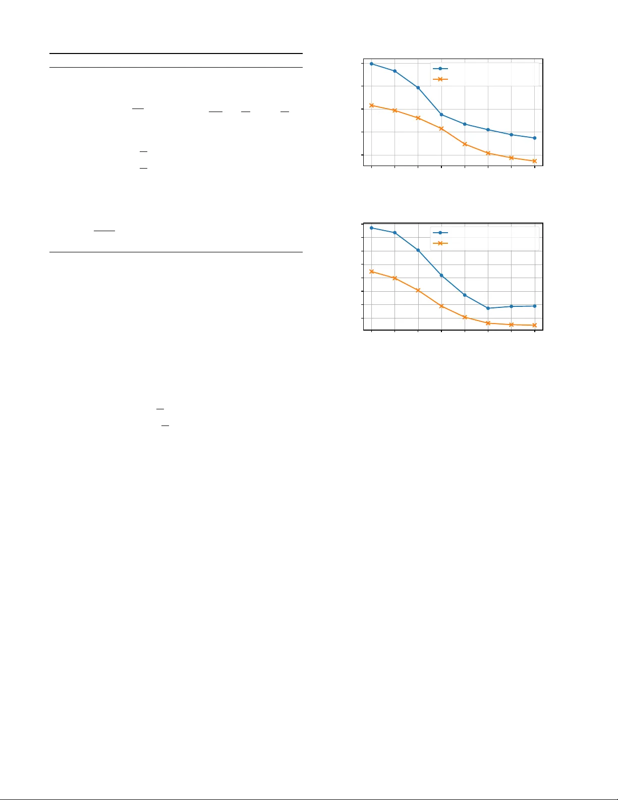
PREPRINT 1 Reconstruction of Piece wise-Constant Sparse Signals for Modulo Sampling Haruka K obayashi and Ryo Hayakawa, Member , IEEE Abstract —Modulo sampling is a promising technology to pre- serve amplitude information that exceeds the observable range of analog-to-digital con verters during the digitization of analog signals. Since con ventional methods typically reconstruct the original signal by estimating the differences of the r esidual signal and computing their cumulative sum, each estimation error inevitably propagates through subsequent time samples. In this paper , to eliminate this error-propagation problem, we propose an algorithm that reconstructs the residual signal directly . The proposed method takes advantage of the high-frequency char - acteristics of the modulo samples and the sparsity of both the residual signal and its difference. Simulation results show that the proposed method reconstructs the original signal mor e accurately than a con ventional method based on the differences of the residual signal. Index T erms —Modulo sampling, dynamic range, unlimited sampling, ADMM. I . I N T R O D U C T I O N S AMPLING plays a fundamental role in modern signal processing. An analog-to-digital con verter (ADC) for sam- pling is typically characterized by two primary performance metrics: the sampling period and the observable amplitude range. When the maximum frequency of the input signal ex- ceeds half of the sampling frequency , aliasing distortion arises during reconstruction [1], [2]. Furthermore, when the signal amplitude exceeds the observable range, the signal is clipped and accurate recov ery of the original signal becomes generally impossible. Signal clipping can cause serious problems in a wide range of practical applications [3], [4]. T o prev ent such distortions, a higher sampling rate or a wider dynamic range is required, which in turn leads to increased po wer consumption. T o balance energy efficienc y and reconstruction accuracy , it is desirable to use an ADC with a lower sampling rate and a narrower dynamic range without causing signal clipping. T o av oid clipping in an ADC with a small observable amplitude range, modulo sampling has been proposed [5]. In modulo sampling, a folding operation is performed by a modulo operator before measurement so that the amplitude of the resulting folded signal lies within [ − λ, λ ) ( λ > 0 ). The folded signal is then sampled by an ADC that can This work will be submitted to the IEEE for possible publication. Copyright may be transferred without notice, after which this version may no longer be accessible. This work was supported in part by The T elecommunications Advancement Foundation and Japan Society for the Promotion of Science (JSPS) KAKENHI under Grant JP24K17277. Haruka Kobayashi is with the Graduate School of Engineering Science, The University of Osaka, 560-8531, Osaka, Japan. Ryo Hayakawa is with the Institute of Engineering, T okyo Univ ersity of Agriculture and T echnology , 184-8588, T okyo, Japan. λ − λ f f λ modulo samples Fig. 1. Illustration of modulo sampling. measure only the range [ − λ, λ ) . Fig. 1 illustrates the concept of modulo sampling. By comparing the original signal f with the folded signal f λ obtained from modulo sampling, we can see that modulo sampling prev ents clipping and preserves the wa veform in part even when the amplitude exceeds the observable range. Howe ver , since we sample the folded signal in modulo sampling, it is necessary to reconstruct the original unfolded signal from these samples. V arious methods have been proposed to reconstruct the original signal from the samples obtained by modulo sam- pling [5]–[16]. A hardware-oriented approach [9] uses a reset count map to record the number of foldings together with the folded signal. This approach, howe ver , requires complex electronic circuitry as well as additional power and memory . As a reconstruction method without the reset count map, an algorithm using high-order differences of the signal has been studied [5], [10]. Subsequently , a prediction-based algorithm has been proposed, demonstrating that in the absence of noise, perfect recovery is possible for finite energy signals at any sampling rate above the Nyquist rate [11]. More recently , a more noise-robust method called beyond bandwidth residual reconstruction ( B 2 R 2 ), which focuses on the high-frequency band of the folded signal, has been proposed [12]. Building on this approach, least absolute shrinkage and selection operator- B 2 R 2 (LASSO- B 2 R 2 ) has been introduced to further improve performance [13]. This method exploits the sparsity of the first-order difference of the residual signal, which represents the number of wraps and is defined as the difference between the signal obtained by modulo sampling and the original signal. Although this approach can reconstruct the signal effi- ciently , reconstruction methods based on the difference of the residual signal suffer from the problem that a reconstruction error at one time index propagates to all subsequent points. In this study , we propose an optimization problem for directly reconstructing the residual signal in modulo sampling. In the proposed residual signal-based optimization problem, we first introduce a regularization term to exploit the sparsity PREPRINT 2 of the first-order difference of the residual signal as in con ven- tional methods. In addition, we newly focus on the sparsity of the residual signal itself and introduce a regularization term that promotes this property as well. T o solve the optimization problem efficiently , we deri ve an algorithm based on the al- ternating direction method of multipliers (ADMM) [17], [18]. Simulation results show that the proposed method achiev es a lower normalized mean squared error (NMSE) than the con ventional LASSO- B 2 R 2 . Throughout this paper , R , C , and Z denote the sets of all real numbers, complex numbers, and integers, respectiv ely . For a vector x = [ x 1 · · · x N ] ⊤ ∈ R N , ∥ x ∥ p = p q P N n =1 | x n | p represents the ℓ p -norm ( p > 0 ). W e denote by I N the N × N identity matrix. The proximal operator of a func- tion ϕ : R N → R ∪ { + ∞} is defined as prox ϕ ( u ) : = arg min v ∈ R N n 1 2 ∥ u − v ∥ 2 2 + ϕ ( v ) o . The operators ⌈·⌉ and ⌊·⌋ denote the ceiling and floor functions, respectiv ely . I I . M O D U L O S A M P L I N G In typical sampling, the signal is clipped when the amplitude of the input signal exceeds the observable amplitude range of the ADC. The clipped signal f cl ( t ) is obtained by limiting the amplitude of f ( t ) to the range [ − λ, λ ] ( λ > 0 ), which is given by f cl ( t ) = min( λ, max( − λ, f ( t ))) . T o avoid clipping, modulo sampling has been proposed [5]. In modulo sampling, the folded signal f λ ( t ) is obtained by applying the following operation to the input f ( t ) as f λ ( t ) = M λ ( f ( t )) = { ( f ( t ) + λ ) mo d 2 λ } − λ. (1) The operation M λ ( · ) folds the signal using the modulo oper- ator when the amplitude of the input signal exceeds [ − λ, λ ) , and confines the signal amplitude within [ − λ, λ ) [12]. The sampled signal f λ [ n ] can be expressed as f λ [ n ] = f λ ( nT s ) , where T s is the sampling period. In modulo sampling, we need to reconstruct the original unfolded signal f [ n ] = f ( nT s ) from the folded samples f λ [ n ] . In the recovery of the original signal f [ n ] , we introduce the residual signal given by z [ n ] : = f λ [ n ] − f [ n ] ( ⇔ f λ [ n ] = f [ n ] + z [ n ]) , (2) which is the difference between the folded signal f λ [ n ] and the original signal. Since f λ [ n ] is known, the problem of reconstructing f [ n ] can be reduced to the reconstruction of the residual signal z [ n ] . I I I . C O N V E N T I O N A L I S T A - B A S E D R E S I D U A L S I G N A L R E C O N S T RU C T I O N A. Pr operties of Modulo Sampling As an ef fectiv e method for recov ering the original signal in modulo sampling, LASSO- B 2 R 2 has been proposed [13]. This method uses the fact that the first-order difference of the residual signal z [ n ] is sparse because z [ n ] is typically piecewise-constant. T o see this, we show an example of the original signal f [ n ] and the corresponding residual signal z [ n ] in Fig. 2. As can be seen from Fig. 2, since z [ n ] often takes the same value consecutively , its first-order difference 2 λ − 2 λ 4 λ − 4 λ 0 f z Fig. 2. An original signal f and its residual signal z ˆ z [ n ] : = z [ n ] − z [ n − 1] becomes a sparse signal with man y zero components. Note that we here define z [ − 1] = 0 to ensure that the lengths of the original and the difference signals are identical. LASSO- B 2 R 2 also uses the properties of modulo sampling in the frequency domain. The frequency spectrum of the original signal f ( t ) is confined to the range [ − ω m , ω m ] , where ω m represents the maximum angular frequency of the signal. On the other hand, the frequency spectrum of the folded signal and the residual signal extends beyond [ − ω m , ω m ] as a result of the signal folding. Thus, it is necessary to set the sampling frequency ω s to be larger than twice the maximum frequency ω m of the signal, i.e., the oversampling f actor (OF) OF = ω s / (2 ω m ) is larger than one. T o analyze the original signal in the frequency domain, we first define discrete Fourier transform (DFT) of f [ n ] as F  e j 2 πk N  = N − 1 X n =0 f [ n ] e − j 2 πk n N , (3) where N is the signal length. Gi ven the relation ω T s = 2 π k / N and ω s = 2 π /T s , the condition for the frequency band where the original signal has no components, i.e., ω m < | ω | < ω s / 2 , is equiv alent to π OF < 2 π k N < 2 π − π OF . (4) For any integer k satisfying (4), we hav e F  e j 2 πk N  = 0 . (5) On the other hand, the frequency spectrum of the folded signal exists not only in the range [ − ω m , ω m ] but also in the higher frequency bands owing to the signal folding effect. Specifically , from (2) and (5), DFT of the folded signal F λ ( e j 2 πk N ) satisfies F λ  e j 2 πk N  = Z  e j 2 πk N  (6) for all integers k satisfying (4). Here, F λ  e j 2 πk N  and Z  e j 2 πk N  are DFTs of the folded signal f λ [ n ] and the residual signal z [ n ] , respectiv ely . Let K be the set of inte gers k that satisfy the condition 2 π k N ∈ ( π OF , 2 π − π OF ) , and let M = |K| be the number of elements in this set. W e consider a partial DFT matrix V ∈ C M × N consisting only of ro ws corresponding to the elements k in the set K . In this matrix, the component specified by PREPRINT 3 a certain k ∈ K and a column index n is giv en by v k,n = e − j 2 πkn N . Then, equation in (6) can be written as F λ = V z . (7) Here, F λ ∈ C M is a vector obtained by arranging the components of DFT of the folded signal f λ [ n ] corresponding to V , and z ∈ R N is a vector obtained by arranging the residual signal z [ n ] . The above discussion holds for the first-order difference of the signals as well. W e define the first-order dif ference ˆ f [ n ] of the signal f [ n ] as ˆ f [ n ] := f [ n ] − f [ n − 1] , as well as the first-order difference of the folded signal f λ [ n ] as ˆ f λ [ n ] := f λ [ n ] − f λ [ n − 1] . By taking the first-order difference of both sides of (2), we have ˆ f λ [ n ] = ˆ f [ n ] + ˆ z [ n ] . At this time, ˆ f [ n ] is band-limited in the same way as f [ n ] , and hence we obtain ˆ F λ = V ˆ z . (8) B. Residual Signal Reconstruction Using IST A In LASSO- B 2 R 2 , the first-order difference ˆ z is recon- structed using (8) and its sparsity . Since the components of ˆ F λ and V are complex numbers, we rewrite (8) into a real-domain equation to construct a recov ery problem in the real domain in this paper . Using the matrices formed by arranging the real and imaginary parts of ˆ F λ and V as ˆ F R λ = h (Re ˆ F λ ) ⊤ (Im ˆ F λ ) ⊤ i ⊤ and V R =  (Re V ) ⊤ (Im V ) ⊤  ⊤ , respectiv ely , complex-valued model in (8) can be rewritten as ˆ F R λ = V R ˆ z . (9) T o recov er ˆ z , LASSO- B 2 R 2 solves the optimization prob- lem based on LASSO [19] for sparse signal recov ery as minimize ˆ z ∈ R N 1 2    ˆ F R λ − V R ˆ z    2 2 + γ ∥ ˆ z ∥ 1 . (10) The first term in (10) is the difference between the observed value ˆ F R λ and V R ˆ z , and the second term is a regularization term to exploit the sparsity of ˆ z . γ ( > 0 ) is a regularization parameter representing the weight of the regularization term. The optimization problem in (10) can be solv ed by the iterati ve shrinkage-thresholding algorithm (IST A) [20], [21]. After the reconstruction of ˆ z , z is obtained by taking the cumulativ e sum of ˆ z as z [ n ] = n X k =0 ˆ z [ k ] for n = 1 , . . . , N . (11) Finally , the estimate of the original signal f [ n ] is obtained from (2). I V . P RO P O S E D R E C O N S T R U C TI O N M E T H O D A. Fused Sparse Reconstruction (FSR) Con ventional approaches such as LASSO- B 2 R 2 suffer from two issues. First, because the reconstruction of the residual signal z in volv es the cumulati ve sum of the estimate of the first-order difference ˆ z as in (11), a reconstruction error in a single element z [ n ] can propagate and permanently contami- nate subsequent estimate of the residual signal z and the orig- inal signal f . T o avoid this error propagation, it is preferable to reconstruct z directly , rather than reconstructing it through ˆ z . In this case, the observation model in (7) can be used to reconstruct z . T o construct a real-domain reconstruction algo- rithm, we consider the matrix F R λ =  (Re F λ ) ⊤ (Im F λ ) ⊤  ⊤ and rewrite (7) as F R λ = V R z . (12) The task is then to reconstruct z from F R λ and V R . The second issue is that some conv entional methods exploit only the sparsity of the first-order dif ference ˆ z of the residual signal, although weak sparsity may exist in z itself. In practice, the residual signal z tends to be sparse when the original signal values are largely concentrated within [ − λ, λ ) , as z [ n ] = 0 whenev er f [ n ] ∈ [ − λ, λ ) . This structural property suggests that incorporating a sparsity-promoting regularization on z itself can improve reconstruction performance. T o address both issues, we propose fused sparse reconstruc- tion (FSR) , which directly recovers z while le veraging the sparsity of both z and its first-order difference. The proposed optimization problem for the reconstruction of z is formulated as minimize z ∈ R N 1 2   F R λ − V R z   2 2 + γ 1 ∥ D z ∥ 1 + γ 2 ∥ z ∥ 1 . (13) Here, D ∈ R N × N is the first-order circular difference matrix, whose entries are d i,j = − 1 if i = j , d i,j = 1 if i = ( j − 1) mo d N , and d i,j = 0 otherwise ( i, j ∈ 0 , 1 , . . . , N − 1 ). The second term ∥ D z ∥ 1 in (13) enforces sparsity on the first-order difference of z , while the third term ∥ z ∥ 1 promotes sparsity in z itself. The positi ve parameters γ 1 and γ 2 are the weights of these two regularizers, respecti vely . B. ADMM-Based Algorithm for FSR For the proposed optimization problem in (13), we deriv e an algorithm based on ADMM [17], [18]. First, by introducing auxiliary variables u 1 ∈ R N and u 2 ∈ R N , we rewrite (13) as minimize z ∈ R N 1 2 ∥ F R λ − V R z ∥ 2 2 + γ 1 ∥ u 1 ∥ 1 + γ 2 ∥ u 2 ∥ 1 sub ject to Dz = u 1 , z = u 2 . (14) By letting u = [ u ⊤ 1 u ⊤ 2 ] ⊤ ∈ R 2 N , Φ = [ D ⊤ I N ] ⊤ ∈ R 2 N × N , f ( z ) = 1 2   F R λ − V R z   2 2 , and g ( u ) = γ 1 ∥ u 1 ∥ 1 + γ 2 ∥ u 2 ∥ 1 , we obtain minimize z ∈ R N , u ∈ R 2 N f ( z ) + g ( u ) sub ject to Φ z = u . (15) The ADMM iterations for (15) are given by z ( i +1) = arg min z ∈ R N n f ( z ) + ρ 2 ∥ Φ z − u ( i ) + y ( i ) ∥ 2 2 o , (16) u ( i +1) = prox 1 ρ g ( Φ z ( i +1) + y ( i ) ) , (17) y ( i +1) = y ( i ) + Φ z ( i +1) − u ( i +1) , (18) where ρ ( > 0 ) is the parameter , i is the iteration index, and y ( i ) ∈ R 2 N is the scaled dual variable. PREPRINT 4 Algorithm 1 Proposed Fused Sparse Reconstruction (FSR) Input: f λ [ n ] (0 ≤ n < N ) , λ, I , OF , N , V R Output: f [ n ] 1: Initialization: γ 1 , γ 2 , ρ > 0 and ˆ z (0) ∼ N (0 , 1) 2: Compute F λ ( e j 2 πk N ) , ∀ k ∈ Z and 2 π k N ∈ ( π OF , 2 π − π OF ) 3: for i = 0 to I − 1 do 4: Compute z ( i +1) via (19) 5: u ( i +1) 1 ← prox γ 1 ρ ∥·∥ 1  D z ( i +1) + y ( i ) 1  6: u ( i +1) 2 ← prox γ 2 ρ ∥·∥ 1  z ( i +1) + y ( i ) 2  7: y ( i +1) 1 ← y ( i ) 1 + D z ( i +1) − u ( i +1) 1 8: y ( i +1) 2 ← y ( i ) 2 + z ( i +1) − u ( i +1) 2 9: end for 10: z ← z ( I ) 11: z ←  ⌊ z /λ ⌋ 2  · 2 λ 12: f [ n ] ← f λ [ n ] − z [ n ] Both updates in (16) and (17) hav e explicit e xpressions. Solving (16) yields z ( i +1) =  ρ ( D ⊤ D + I N ) + V R ⊤ V R  − 1 ·  ρ D ⊤ ( u ( i ) 1 − y ( i ) 1 ) + ρ ( u ( i ) 2 − y ( i ) 2 ) + V R ⊤ F R λ  . (19) Here, y 1 ∈ R N and y 2 ∈ R N are v ariables obtained by partitioning y such that y = [ y ⊤ 1 y ⊤ 2 ] ⊤ , in the same manner as u . The update in (17) decouples as u ( i +1) = " pro x γ 1 ρ ∥·∥ 1 ( D z ( i +1) + y ( i ) 1 ) pro x γ 2 ρ ∥·∥ 1 ( z ( i +1) + y ( i ) 2 ) # . (20) The proximal operator for the ℓ 1 norm becomes an element- wise soft-thresholding function gi ven by prox τ ∥·∥ 1 ( x ) = sign( x ) max( | x | − τ , 0) , where sign( · ) is the sign function. After we obtain the estimate of z , we apply a rounding operation to enforce the estimate to be an inte ger multiple of 2 λ . The proposed reconstruction algorithm is presented in Algorithm 1. The computational cost of Algorithm 1 is dominated by the update step for z in (19). A straightforward implementation of this step would require a matrix in version, resulting in a computational cost of O ( N 3 ) . Howe ver , since the in verse matrix admits the closed-form expression ( ρ ( D ⊤ D + I N ) + V R ⊤ V R ) − 1 = F H ( ρ ( Λ D + I ) + Λ V ) − 1 F with the in verse of a diagonal matrix, the computational complexity per iter- ation becomes O ( N log N ) . Detailed deri vations are giv en in Appendix. V . S I M U L A T I O N R E S U LT S W e ev aluate the performance of the proposed method via computer simulations. A test signal with maximum frequency 1 /T s × 1 / OF is first generated by superposing five random sine wa ves whose amplitudes, frequencies, and phases drawn independently from uniform distrib utions. This composite wa veform is then normalized so that its maximum amplitude becomes 1 . Modulo sampling with width λ = 0 . 25 is applied to this signal. Zero-mean Gaussian noise generated according 0 5 10 15 20 25 30 35 SNR [dB] − 20 − 10 0 10 20 NMSE [dB] LASSO- B 2 R 2 (Conv entional) FSR (Proposed) Fig. 3. Reconstruction results for OF = 6 . 2 3 4 5 6 7 8 9 OF − 15 − 10 − 5 0 5 10 15 20 NMSE [dB] LASSO- B 2 R 2 (Conv entional) FSR (Proposed) Fig. 4. Reconstruction results for SNR = 20 dB. to each specified signal-to-noise ratio (SNR) is added to the signal. For each noisy signal, the reconstruction is performed 250 times, and the av eraged NMSE between the original and reconstructed signals giv en by NMSE = ∥ f − f est ∥ 2 2 / ∥ f ∥ 2 2 is ev aluated, where f = [ f [0] , . . . , f [ N − 1]] ⊤ ∈ R N denotes the original signal and f est is the corresponding reconstructed signal. The parameters are set to N = 1024 , T s = 0 . 01 , I = 150 , γ 1 = 1 , γ 2 = 0 . 01 and ρ = 2 . 0 . Fig. 3 shows the NMSE performance when OF is 6 and SNR is varied from 0 to 35 dB. Fig. 4 plots the NMSE performance when SNR is 20 dB and OF is varied from 2 to 9 . From the figures, we can see that the proposed method consistently achiev es a smaller NMSE than LASSO- B 2 R 2 , which achiev es better performance than several other con ventional methods [13]. This improv ement is attributed to the promotion of sparsity in z by the new regularization term and to the elimination of error propagation achie ved by directly recov ering z . V I . C O N C L U S I O N In this study , we have proposed an optimization problem that directly reconstructs the residual signal for signal re- construction in modulo sampling. The proposed formulation exploits both the high-frequency characteristics of the sampled data and two types of sparsity: in the residual signal itself and in its first-order difference. For the proposed optimiza- tion problem, we have deri ved an efficient ADMM-based algorithm. Computer simulations have demonstrated that the proposed method achieves superior reconstruction accuracy ov er the conv entional LASSO- B 2 R 2 . PREPRINT 5 A P P E N D I X This appendix describes the efficient computation of the in verse matrix of A : = ρ ( D ⊤ D + I ) + V R ⊤ V R (21) used in the z -update step of the proposed algorithm. W e will sho w that we can efficiently multiply A − 1 to a vector b (i.e., compute x = A − 1 b ) with O ( N log N ) complexity by exploiting the diagonalization properties of the constituent matrices. A. Diagonalization of the Differ ence Matrix Assuming periodic boundary conditions, the difference ma- trix D is a circulant matrix, and thus D ⊤ D is also circulant. It can be diagonalized by the normalized discrete Fourier transform (DFT) matrix F ∈ C N × N as D ⊤ D = F H Λ D F , where ( · ) H denotes the Hermitian transpose. The k -th diagonal element of Λ D is given by λ D,k =    1 − e − j 2 πk N    2 = 4 sin 2  π k N  . (22) B. Diagonalization of the Observation Matrix T o diagonalize the second term V R ⊤ V R using the DFT matrix, we first establish the relationship between V R and the complex observation matrix V = Re V + j Im V ∈ C M × N . The real-valued observation matrix V R is defined by stacking the real and imaginary parts as V R : =  Re V Im V  ∈ R 2 M × N . (23) A ke y identity relates this real Gram matrix to the complex one: V R ⊤ V R = (Re V ) ⊤ (Re V ) + (Im V ) ⊤ (Im V ) (24) = Re( V H V ) . (25) Now , consider the case of partial Fourier sensing, where V = S F with a row-selection matrix S . In this case, V H V = F H Λ mask F , where Λ mask = S ⊤ S is a diagonal sampling mask. Substituting this into (25) yields V R ⊤ V R = Re( F H Λ mask F ) = 1 2  F H Λ mask F + ( F H Λ mask F ) ∗  , (26) where ( · ) ∗ denotes the complex conjugate. Let Π ∈ R N × N be the frequency-re versal permutation matrix defined by [ Π ] k,ℓ = ( 1 , ℓ = ( − k ) N , 0 , otherwise , ( − k ) N : = ( − k ) mo d N . (27) Then Π ⊤ = Π − 1 = Π . F or the normalized DFT matrix [ F ] m,n = 1 √ N e − j 2 πmn N , we have [ Π F ] m,n = [ F ] ( − m ) N ,n = 1 √ N e − j 2 π ( − m ) n N = [ F ∗ ] m,n , (28) hence Π F = F ∗ and therefore F ⊤ = ( F ∗ ) H = ( Π F ) H = F H Π . Since Λ mask is real diagonal, we hav e ( F H Λ mask F ) ∗ = ( F H ) ∗ Λ ∗ mask F ∗ = F ⊤ Λ mask F ∗ = ( F H Π ) Λ mask ( Π F ) = F H ( ΠΛ mask Π ) F . (29) Thus, the observation term is diagonalized by the DFT matrix as V R ⊤ V R = F H Λ V F , (30) where the diagonal matrix Λ V is defined as Λ V : = Λ mask + ΠΛ mask Π 2 . (31) The k -th diagonal element λ V ,k of Λ V is therefore giv en by the average of the mask at symmetric frequencies as λ V ,k = λ mask ,k + λ mask , ( − k ) N 2 , (32) where λ mask ,k is the k -th diagonal element of Λ mask . C. Summary of F ast In version Since both D ⊤ D and V R ⊤ V R are simultaniously diago- nalized by F , the matrix A is expressed as A = F H ( ρ ( Λ D + I ) + Λ V ) F (33) = F H Λ A F , (34) where Λ A = ρ ( Λ D + I ) + Λ V is the diagonal matrix. From (34), we hav e A − 1 = F H Λ − 1 A F . Thus, multiplication by A − 1 can be computed via FFT , element-wise division by the diagonal entries of Λ A , and IFFT . The ov erall computa- tional complexity is reduced to O ( N log N ) from O ( N 3 ) for the straightforward implementation. R E F E R E N C E S [1] Y . C. Eldar , Sampling Theory: Beyond Bandlimited Systems . Cambridge Univ ersity Press, Apr . 2015. [2] M. Mishali and Y . C. Eldar , “Sub-Nyquist Sampling, ” IEEE Signal Pr ocessing Magazine , vol. 28, no. 6, pp. 98–124, Jan. 2011. [3] K. Y amada, T . Nakano, and S. Y amamoto, “A V ision Sensor Having an Expanded Dynamic Range for Autonomous V ehicles, ” IEEE T ransac- tions on V ehicular T echnology , vol. 47, no. 1, pp. 332–341, Feb . 1998. [4] F . Bie, D. W ang, J. W ang, and T . F . Zheng, “Detection and Reconstruc- tion of Clipped Speech for Speaker Recognition, ” Speech Communica- tion , vol. 72, pp. 218–231, Sep. 2015. [5] A. Bhandari, F . Krahmer , and R. Raskar , “On Unlimited Sampling and Reconstruction, ” IEEE T ransactions on Signal Pr ocessing , vol. 69, pp. 3827–3839, 2021. [6] S. Rudresh, A. Adiga, B. A. Shenoy , and C. S. Seelamantula, “W avelet- Based Reconstruction for Unlimited Sampling, ” in Proceedings of IEEE International Conference on Acoustics, Speech and Signal Pr ocessing (ICASSP) , Apr. 2018, pp. 4584–4588. [7] A. Bhandari, F . Krahmer, and R. Raskar, “Unlimited Sampling of Sparse Signals, ” in Pr oceedings of IEEE International Conference on Acoustics, Speech and Signal Pr ocessing (ICASSP) , Apr . 2018, pp. 4569–4573. [8] D. Prasanna, C. Sriram, and C. R. Murthy , “On the Identifiability of Sparse V ectors From Modulo Compressed Sensing Measurements, ” IEEE Signal Pr ocessing Letters , vol. 28, pp. 131–134, 2021. PREPRINT 6 [9] K. Sasagawa, T . Y amaguchi, M. Haruta, Y . Sunaga, H. T akehara, H. T akehara, T . Noda, T . T okuda, and J. Ohta, “ An Implantable CMOS Image Sensor With Self-Reset Pixels for Functional Brain Imaging, ” IEEE T ransactions on Electr on Devices , vol. 63, no. 1, pp. 215–222, Jan. 2016. [10] A. Bhandari, F . Krahmer , and R. Raskar, “On Unlimited Sampling, ” in Proceedings of International Confer ence on Sampling Theory and Applications (SampTA) , Jul. 2017, pp. 31–35. [11] E. Romanov and O. Ordentlich, “ Above the Nyquist Rate, Modulo Folding Does Not Hurt, ” IEEE Signal Pr ocessing Letters , vol. 26, no. 8, pp. 1167–1171, Aug. 2019. [12] E. Azar, S. Mulleti, and Y . C. Eldar , “Residual Recov ery Algorithm for Modulo Sampling, ” in Proceedings of IEEE International Conference on Acoustics, Speech and Signal Pr ocessing (ICASSP) , May 2022, pp. 5722–5726. [13] S. B. Shah, S. Mulleti, and Y . C. Eldar, “Lasso-Based Fast Residual Recovery For Modulo Sampling, ” in Pr oceedings of IEEE International Confer ence on Acoustics, Speec h and Signal Processing (ICASSP) , Jun. 2023, pp. 1–5. [14] A. Bhandari, F . Krahmer, and T . Poskitt, “Unlimited Sampling From Theory to Practice: Fourier -Prony Recovery and Prototype ADC, ” IEEE T ransactions on Signal Processing , vol. 70, pp. 1131–1141, 2022. [15] D. Florescu, F . Krahmer, and A. Bhandari, “Unlimited Sampling with Hysteresis, ” in Pr oceedings of 55th Asilomar Conference on Signals, Systems, and Computers , Oct. 2021, pp. 831–835. [16] D. Florescu and A. Bhandari, “Unlimited Sampling via Generalized Thresholding, ” in Proceedings of IEEE International Symposium on Information Theory (ISIT) , Jun. 2022, pp. 1606–1611. [17] J. Eckstein and D. P . Bertsekas, “On the Douglas–Rachford Splitting Method and the Proximal Point Algorithm for Maximal Monotone Operators, ” Mathematical pr ogramming , vol. 55, no. 1-3, pp. 293–318, Apr . 1992. [18] S. Boyd, “Distributed Optimization and Statistical Learning via the Alternating Direction Method of Multipliers, ” F oundations and T rends® in Machine Learning , vol. 3, no. 1, pp. 1–122, 2010. [19] R. Tibshirani, “Regression Shrinkage and Selection via the Lasso, ” Journal of the Royal Statistical Society: Series B (Methodological) , vol. 58, no. 1, pp. 267–288, Jan. 1996. [20] I. Daubechies, M. Defrise, and C. De Mol, “An Iterative Thresholding Algorithm for Linear Inv erse Problems with a Sparsity Constraint, ” Communications on Pure and Applied Mathematics , vol. 57, no. 11, pp. 1413–1457, Nov . 2004. [21] P . L. Combettes and V . R. W ajs, “Signal Recovery by Proximal Forw ard- Backward Splitting, ” Multiscale Modeling & Simulation , vol. 4, no. 4, pp. 1168–1200, Jan. 2005.