Two-way Clustering Robust Variance Estimator in Quantile Regression Models

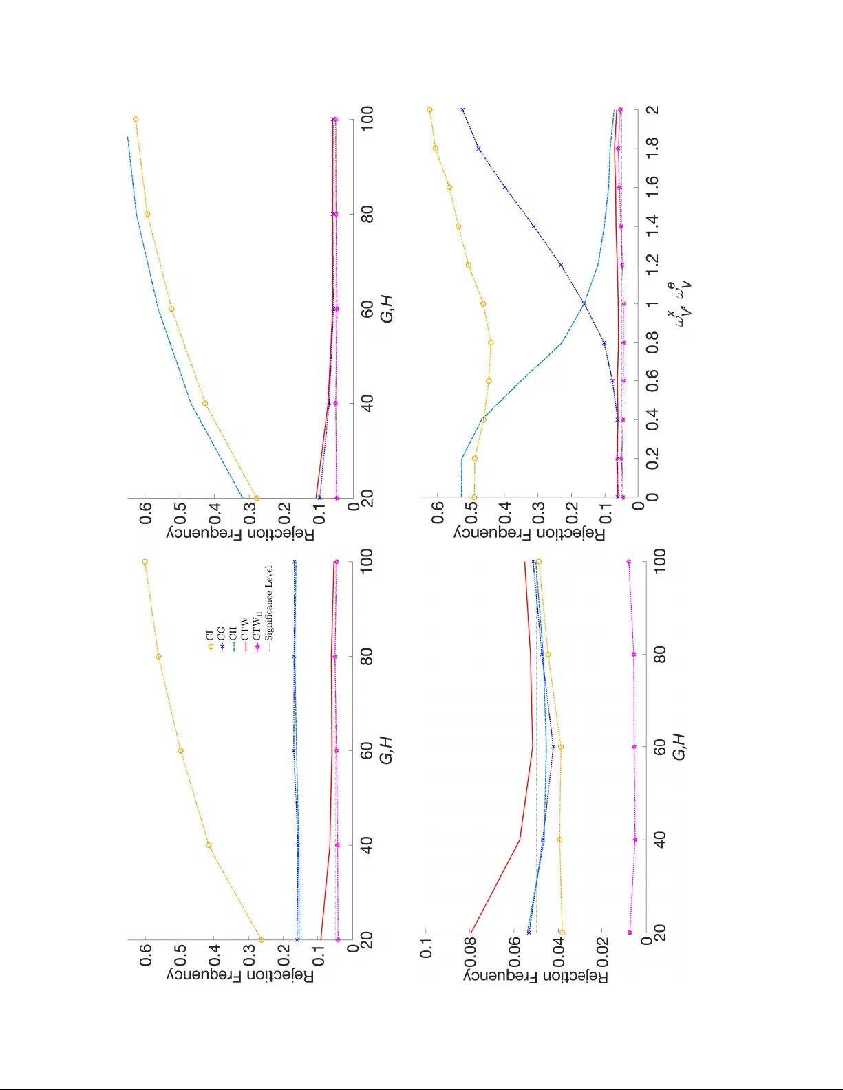
T w o-w a y Clustering Robust V ariance Estimator in Quan tile Regression Mo dels ∗ Ulric h Houn y o † Jiahao Lin ‡ F ebruary 19, 2026 Abstract W e study inference for linear quan tile regression with t wo-w ay clustered data. Us- ing a separately exc hangeable arra y framew ork and a pro jection decomposition of the quan tile score, w e characterize regime-dependent con vergence rates and establish a self-normalized Gaussian approximation. W e prop ose a t wo-w ay cluster-robust sand- wic h v ariance estimator with a kernel-based densit y “bread” and a pro jection-matc hed “meat”, and pro v e consistency and v alidity of inference in Gaussian regimes. W e also sho w an impossibility result for uniform inference in a non-Gaussian interaction regime. JEL Classiﬁcation : C15, C23, C31, C80 Keyw ords : Clustered data, cluster-robust v ariance estimator, t wo-w a y clustering, quan tile regression. ∗ W e are grateful for the helpful commen ts pro vided b y An tonio F. Galv ao, Carlos Lamarche, Harold Chiang, and Y uya Sasaki. All the remaining errors are ours. † Departmen t of Economics, Univ ersit y at Albany – State Universit y of New Y ork, Alban y , NY 12222, United States. ‡ Departmen t of Economics, Univ ersit y at Albany – State Universit y of New Y ork, Alban y , NY 12222, United States. 1 In tro duction Quan tile regression (QR), introduced b y Koenker and Bassett Jr ( 1978 ), is a widely used to ol for studying heterogeneous eﬀects and tail risks in economics and ﬁnance. In many empirical en vironments, ho w ever, observ ations are indexed by m ultiple clustering dimen- sions and exhibit dep endence along each of them. A canonical example is a t w o-w ay arra y { ( y g h , X g h ) : g = 1 , . . . , G, h = 1 , . . . , H } in which observ ations can b e correlated within the g -dimension and within the h -dimension because of laten t sho cks shared by units in the same ro w or column (e.g., w orker × ﬁrm, exporter × destination). This paper dev elops a uniﬁed large-sample theory and feasible inference pro cedures for linear QR under t wo-w a y clustering. W e study the conditional quan tile regression mo del and allo w for ric h tw o-w a y dependence using an Aldous–Hoov er–Kallen b erg (AHK) represen ta- tion for separately exchangeable arrays ( Aldous , 1981 ; Hoov er , 1979 ; Kallen b erg , 1989 ). This framew ork has become a standard device for mo deling m ulti-w ay clustered dep endence and for deriving pro jection-based asymptotics for array data (e.g., Da vezies et al. , 2021 ; Menzel , 2021 ; Chiang et al. , 2024 ; Graham , 2024 ). Building on this structure, w e establish a self- normalized cen tral limit theorem that accommo dates regime-dep enden t rates and deliv ers asymptotic normalit y . W e then propose a feasible t w o-wa y cluster-robust v ariance estimator (CR VE) for QR of the familiar sandwich form b Σ( τ ) = b D ( τ ) − 1 b Ω( τ ) b D ( τ ) − 1 . The “bread” b D ( τ ) is a k ernel-based estimator of the conditional densit y at the target quantile, adapted here to tw o-wa y clustering, while the “meat” b Ω( τ ) aggregates ro w- and column- cluster cov ariance con tributions along with a residual comp onent in a manner that mirrors the underlying pro jection decomposition. F our features fundamen tally complicate establishing the consistency of b Σ( τ ) relativ e to standard tw o-w ay clustered mean regression (e.g., Cameron et al. 2011 ; MacKinnon et al. 2021 ) and to one-w ay clustered quan tile regression (e.g., Paren te and Santos Silv a 2016 ; Hage- mann 2017 ). First, unlik e mean regression, the quan tile score is non-smooth, whic h mak es uniform con trol of score ﬂuctuations in neighborho o ds of β 0 ( τ ) more delicate. Second, the Jacobian depends on the conditional density at zero and is estimated nonparametrically , so the pro of m ust con trol the bias and sto chastic error of a k ernel-based “bread” under clus- tering. Third, unlik e one-w a y clustered quan tile regression, the eﬀective con vergence rate of b β ( τ ) , denoted r GH , can v ary across dep endence regimes: dep ending on the relativ e magni- tudes of the ro w, column, and in teraction comp onen ts of the score, diﬀeren t pro jection terms ma y dominate the leading stochastic ﬂuctuation. F ourth, tw o-wa y dep endence precludes re- 2 ducing the sample score to a sum of indep endent (or w eakly dep enden t) terms along either dimension without explicitly isolating the ro w, column, and in teraction components. More imp ortan tly , these four diﬃculties are not additiv e. In our setting, non-smo oth scores and k ernel Jacobian estimation m ust b e handled simultane ously with regime-dep enden t rates and genuinely t w o-wa y dependence, requiring a uniform analysis of both the score and the Jacobian that remains v alid across dependence regimes. Mon te Carlo results conﬁrm that conv en tional QR standard errors can severely understate uncertain ty when t wo-w ay clustering is presen t, whereas the prop osed CR VE delivers reliable co verage across a wide range of dependence conﬁgurations, including one-wa y clustering and cluster-indep enden t settings. F urthermore, w e c haracterize the b oundary of uniform inference. When the in teraction comp onen t remains asymptotically non-negligible while the ro w and column comp onents are w eak, the limiting distribution of b β ( τ ) ma y b e non-Gaussian. In this regime, the distribution of the normalized estimator dep ends sensitively on the underlying DGP . W e show that ov er a natural class of tw o-w ay clustered triangular arra ys, no pro cedure can uniformly consisten tly appro ximate the asymptotic distribution of b β ( τ ) . Uniform inference o ver the full mo del class is therefore unattainable without additional structure. In an empirical application, we study ho w teac her-licensing stringency relates to the supply of high-qualit y teac hers. Consisten t with prior evidence, we ﬁnd little indication that stricter licensing aﬀects high-qualit y candidates on a v erage. Ho wev er, this av erage pattern masks substan tial heterogeneit y: a negativ e eﬀect is concentrated in the lo wer part of the distribution of high-qualit y outcomes, suggesting that some relativ ely strong candidates are close to the margin betw een teaching and other careers and are therefore sensi tiv e to increases in licensing costs. In contrast, for the higher quan tiles w e ﬁnd little evidence that increased stringency discourages right-tail teacher. Recen tly and indep enden tly , Chiang et al. ( 2024 ) study extremal quan tiles under tw o-w ay clustered dep endence, focusing on rare-even t estimation in tw o-w a y clustered data. While Menzel ( 2021 ) show that sample means may exhibit non-Gaussian limits under t w o-wa y clustering, Chiang et al. ( 2024 ) demonstrate that extremal quan tiles can remain robust ev en in degenerate dep endence regimes. Our pap er complements this line of w ork b y fo cusing on interior quan tiles: while Chiang et al. ( 2024 ) analyze b β ( τ ) as τ → 0 , w e consider ﬁxed τ ∈ (0 , 1) , where the non-smo oth quantile score and the interaction of ro w and column comp onen ts hav e fundamen tally diﬀerent implications for the limiting distribution and the v alidity of inference. More broadly , our results con tribute to the literature on robust quantile regression infer- ence under dep endence, including kernel-based theory under weak dep endence ( Kato , 2012 ), 3 CR VE and pigeonhole bo otstrap results for GMM (e.g. quan tile IV) under multiw a y clus- tering ( Dav ezies et al. , 2018 ), and recen t adv ances in w eak-dep endence-robust co v ariance estimation for quantile regression ( Galv ao and Y o on , 2024 ). Relativ e to these pap ers, our con tributions are threefold. First, w e establish asymptotic normalit y of P ow ell’s kernel estimator under tw o-w ay clustering, and deriv e a feasible optimal bandwidth rule. Second, to the best of our kno wledge, w e pro vide the ﬁrst fe asible t wo-w a y cluster-robust v ariance estimator for quan tile regression at a ﬁxed τ ∈ (0 , 1) , and pro ve its uniform v alidity whenever the Gaussian limit arises. Although Da v ezies et al. ( 2018 ) prop ose m ultiwa y v ariance estimation for GMM, their approach is not directly applicable here b ecause it relies on a plug-in Jacobian that requires kno wledge of the true conditional densit y , whic h is t ypically unav ailable in practice. Moreo ver, unlike the setting emphasized in Da vezies et al. ( 2018 ), we do not imp ose nondegeneracy of the asymptotic v ariance: the rate of con vergence is allo wed to v ary with the strength of clustering, and our v ariance estimator is designed to adapt across these regimes. Third, when the limiting distribution in t w o-wa y clustered quan tile regression is non-Gaussian, w e show that uniform consistency of inference is impossible. The remainder of the pap er is organized as follows. Section 2 introduces the t w o-wa y QR framew ork and the pro jection decomposition and develops the regime-adaptiv e limit theory for b β ( τ ) . Section 3 proposes b D ( τ ) and b Ω( τ ) and establishes the consistency of b Σ( τ ) and the v alidit y of inference based on the t -statistic. Section 4 presents Monte Carlo evidence. Section 5 studies an application to teacher licensing. Section 6 concludes. T ec hnical pro ofs and additional results are deferred to the appendix. 2 T w o-W a y Clustering in Quan tile Regression 2.1 Mo del Setting Let { ( y g hi , X ⊤ g hi ) : g = 1 , . . . , G, h = 1 , . . . , H , i = 1 , . . . , N g h } b e an array of observ ations, where y g hi ∈ R is the scalar resp onse and X g hi ∈ R d is a v ector of regressors. The ﬁrst index g iden tiﬁes the cluster in the ﬁrst dimension (the g -cluster), and the second index h iden tiﬁes the cluster in the second dimension (the h -cluster). The index pair ( g , h ) therefore lab els a cell formed b y the intersection of a g -cluster and an h -cluster (e.g., unit × time). Let N g h ∈ N denote the num b er of observ ations within cell ( g , h ) . Fix a quantile index τ ∈ (0 , 1) . W e consider the quan tile regression model Q y ghi ( τ | X g hi ) = X ⊤ g hi β 0 ( τ ) , g = 1 , . . . , G, h = 1 , . . . , H, i = 1 , . . . , N g h , (2.1) 4 where Q y ghi ( τ | X g hi ) denotes the conditional τ -quan tile of y g hi giv en X g hi . The quan tile error e g hi ( τ ) is deﬁned as e g hi ( τ ) := y g hi − X g hi β 0 ( τ ) . Let ρ τ ( u ) := u  τ − 1 { u ≤ 0 }  denote the c heck loss. F or t w o-wa y clustered data, the QR estimator minimizes ˆ β ( τ ) := arg min β ∈ Θ 1 GH G X g =1 H X h =1 N gh X i =1 ρ τ  y g hi − X ⊤ g hi β  , with respect to β ∈ Θ ⊂ R d , where Θ is compact. F or later use, deﬁne the quan tile score ψ g hi ( β , τ ) := X g hi  τ − 1 { y g hi ≤ X ⊤ g hi β }  , Ψ g hi ( τ ) := ψ g hi  β 0 ( τ ) , τ  . (2.2) The function Ψ g hi ( τ ) is nonlinear due to the indicator function, whic h plays a central role in the asymptotic analysis. F or each cell ( g , h ) , let X g h b e the N g h × d matrix with i th ro w X g hi , and let y g h and e g h ( τ ) b e the corresponding N g h × 1 v ectors with i th elemen ts y g hi and e g hi ( τ ) . W e imp ose the conditional quan tile restriction Q e gh ( τ | X g h ) = 0 , i.e., the conditional τ -quan tile of e g h ( τ ) given X g h equals zero. F or simplicity , we fo cus on the case where eac h cell con tains exactly one observ ation, that is, N g h = 1 for all g , h , and suppress the replicate index i . Extensions to heterogeneous N g h are pro vided in the In ternet Appendix. In the t wo-w ay clustering literature, the Aldous–Hoov er–Kallen b erg (AHK) representa- tion is widely used; see, for example, Da vezies et al. ( 2021 ), MacKinnon et al. ( 2021 ), and Chiang et al. ( 2024 ). Assumption 1 (T wo-w a y clustered data with the AHK representation) . Ther e exist me a- sur able functions Γ such that ( y g h , X g h ) = Γ( U g , V h , W g h ) , wher e { U g } g ≥ 1 , { V h } h ≥ 1 , and { W g h } g ,h ≥ 1 ar e mutual ly indep endent se quenc es of i.i.d. r andom variables. Without loss of gener ality, e ach latent variable is uniformly distribute d on [0 , 1] . The function Γ may vary with ( G, H ) , al lowing for triangular-arr ay se quenc es of DGPs. Under Assumption 1 , the array ( y g h , X g h ) is separately exc hangeable across ( g , h ) , and hence marginally identically distributed, though generally dependent. The quan tile index τ aﬀects the mo del only through the conditional quantile restriction and do es not en ter the regressor pro cess. There exists a measurable function Ψ( U, V , W ; τ ) suc h that Ψ g h ( τ ) = Ψ( U g , V h , W g h ; τ ) . The score then admits the Ho eﬀding t yp e decomp osition Ψ g h ( τ ) = E [Ψ g h ( τ )] + Ψ (I) ( U g , τ ) + Ψ (II) ( V h , τ ) + Ψ (II I) ( U g , V h , τ ) + Ψ (IV) ( U g , V h , W g h , τ ) , (2.3) 5 where Ψ ( I ) ( U g , τ ) := E [Ψ g h ( τ ) | U g ] − E [Ψ g h ( τ )] , Ψ ( II ) ( V h , τ ) := E [Ψ g h ( τ ) | V h ] − E [Ψ g h ( τ )] , Ψ ( II I ) ( U g , V h , τ ) := E [Ψ g h ( τ ) | U g , V h ] − E [Ψ g h ( τ )] − Ψ ( I ) ( U g , τ ) − Ψ ( II ) ( V h , τ ) , Ψ ( IV ) ( U g , V h , W g h , τ ) := Ψ g h ( τ ) − E [Ψ g h ( τ ) | U g , V h ] . This decomposition follows from L 2 pro jection theory for separately exchangeable arrays and is unique in L 2 . Closely related decomp ositions for nonlinear statistics under AHK dep endence ha ve b een dev elop ed recen tly for U-statistics on bipartite and ro w–column ex- c hangeable arrays; see Le Minh et al. ( 2025 ). When con venien t, w e write Ψ ( j ) • for Ψ ( j ) ( · ; τ ) , j = I , . . . , IV. W e suppress the dependence on τ to conserv e space. By construction, E [Ψ ( j ) ] = 0 for eac h j and E [Ψ ( j ) • Ψ ( j ′ ) ⊤ • ] = 0 for j  = j ′ . Although ( U g , V h , W g h ) are independent, the comp onents Ψ ( I ) g , Ψ ( II ) h , Ψ ( II I ) g h , and Ψ ( IV ) g h need not be. These comp onents are, how ever, pairwise orthogonal in L 2 , whic h suﬃces to c haracterize asymptotic v ariances and limit distributions. Let f e | X ( e | x ) denote the conditional densit y of e g h giv en X g h = x . f (1) e | X ( e | x ) and f (2) e | X ( e | x ) denote the corresp onding ﬁrst and second deriv ativ es, resp ectively . W e imp ose a natural t wo-w ay arra y analogue of the standard momen t, smo othness, and nonsingularity conditions used in i.i.d. quan tile regression. Assumption 2 (Momen ts, smoothness, and nonsingularit y) . (i) E [Ψ g h ] = 0 , E ∥ X g h ∥ 4 < ∞ , and E ( X g h X ⊤ g h ) is nonsingular. (ii) The map e 7→ f e | X ( e | x ) is twic e c ontinuously diﬀer en- tiable for every x , and sup e,x   f e | X ( e | x )   < ∞ as wel l as sup e,x   f (1) e | X ( e | x )   < ∞ . (iii) The c onditional density at zer o is uniformly b ounde d away fr om zer o: inf x f e | X (0 | x ) > 0 . (iv) The Jac obian matrix E  f e | X (0 | X g h ) X g h X ⊤ g h  and the sc or e varianc e E  Ψ g h Ψ ⊤ g h  ar e p ositive deﬁnite. (v) β 0 ( τ ) lies in the interior of a c omp act p ar ameter sp ac e Θ . 2.2 Asymptotic Distribution F or j ∈ { I , I I , I I I , IV } , deﬁne the comp onent v ariances σ 2 j, Γ := E  Ψ ( j ) Ψ ( j ) ⊤  . The subscript Γ emphasizes that these quan tities depend on the underlying DGP and may v ary with ( G, H ) . T o simplify notation, w e suppress the explicit ( G, H ) dependence. F or eac h j , we further assume, for expositional con venience, that the diagonal elemen ts of σ 2 j, Γ 6 are of the same order; we use the ﬁrst diagonal en try , σ 2 j, 1Γ , to represent this order. A standard argument yields the Bahadur representation ˆ β − β 0 ( τ ) + o P    ˆ β − β 0 ( τ )    = D ( τ ) − 1 ¯ Ψ GH , where D ( τ ) := E  f e | X (0 | X g h ) X g h X ⊤ g h  , ¯ Ψ GH := 1 GH G X g =1 H X h =1 Ψ g h . Using ( 2.3 ), w e decompose ¯ Ψ GH as ¯ Ψ GH = 1 G G X g =1 Ψ ( I ) g + 1 H H X h =1 Ψ ( II ) h + 1 GH G X g =1 H X h =1  Ψ ( II I ) g h + Ψ ( IV ) g h  := ¯ Ψ ( I ) + ¯ Ψ ( II ) + ¯ Ψ ( II I ) + ¯ Ψ ( IV ) . Conditional on the laten t v ariables, the arrays { Ψ (I) g } G g =1 and { Ψ (II) h } H h =1 are i.i.d. across clusters, and, conditional on { U g , V h } , { Ψ (IV) g h } g ,h are i.i.d. across cells. Consequently , after appropriate normalization, the sums asso ciated with ¯ Ψ ( I ) , ¯ Ψ ( II ) , and ¯ Ψ ( IV ) are asymptotically Gaussian, whereas ¯ Ψ ( II I ) ma y admit a non-Gaussian limit. Let the asymptotic v ariance of ˆ β b e Σ GH := D ( τ ) − 1 Ω GH ( τ ) D ( τ ) − 1 , Ω GH ( τ ) := V ar  ¯ Ψ GH  . By orthogonalit y of the ANO V A comp onents, Ω GH ( τ ) = 1 GH  H σ 2 I , Γ + Gσ 2 II , Γ + σ 2 II I , Γ + σ 2 IV , Γ  . (2.4) Assumption 3 (Orders of v ariance comp onents) . (i) The total varianc e do es not vanish: lim inf G,H →∞  H σ 2 I , 1Γ + Gσ 2 II , 1Γ + σ 2 II I , 1Γ + σ 2 IV , 1Γ  > 0 . (ii)A long any subse quenc e indexe d by ( G n , H n ) for which  H n σ 2 I , 1Γ , G n σ 2 II , 1Γ , σ 2 II I , 1Γ , σ 2 IV , 1Γ  c onver ges in [0 , ∞ ] 4 , at le ast one of the fol lowing holds: (a) H n σ 2 I , 1Γ + G n σ 2 II , 1Γ → ∞ , or (b) σ 2 II I , 1Γ → 0 . Assumption 3 (i) guarantees that the asymptotic v ariance of ˆ β is not iden tically zero, although some comp onen ts of the v ariance decomp osition ma y b e absen t. Assumption 3 (ii) 7 rules out non-Gaussian limits driv en b y the in teraction comp onen t. Sp eciﬁcally , either (a) clustering along at least one dimension is suﬃciently strong so that the Gaussian comp onents ¯ Ψ (I) + ¯ Ψ (II) dominate, or (b) the interaction v ariance σ 2 II I , 1Γ is asymptotically negligible, whic h suppresses the p oten tially non-Gaussian con tribution of ¯ Ψ (II I) . In either case, the normalized score admits a Gaussian limit. W e imp ose these conditions along an y con vergen t subsequence, since the original sequence need not conv erge. This allows us to establish uniform v alidity along subsequence. Note that w e do not restrict the relativ e growth rate b et w een G and H . Theorem 2.1. L et B 0 denote the c ol le ction of DGPs Γ that satisfy Assumptions 1 – 3 . Then Σ − 1 / 2 GH  ˆ β − β 0 ( τ )  d → N (0 , I d ) uniformly over Γ ∈ B 0 . Theorem 2.1 establishes asymptotic normalit y under self-normalization. This normaliza- tion accommo dates the p ossibilit y that the con vergence rate of ˆ β v aries with the clustering structure. In particular, Theorem 2.1 and equation ( 2.4 ) together imply that the (infeasible) con vergence rate of b β ( τ ) is r 1 / 2 GH , where r GH := min ( G σ 2 I , 1Γ , H σ 2 II , 1Γ , GH ) . Here, the rate is determined b y the pro jection component that dominates the v ariance de- comp osition in ( 2.4 ). In particular, under standard one-w ay clustering (e.g., along the ﬁrst dimension), where σ 2 I , 1Γ is ﬁxed and positive deﬁnite and σ 2 II , 1Γ = 0 , the rate reduces to G . Under i.i.d. sampling, where σ 2 I , 1Γ = σ 2 II , 1Γ = 0 , it reduces to GH . 3 Cluster-Robust V ariance Estimator (CR VE) The t wo-w a y cluster-robust v ariance estimator for quan tile regression tak es the usual sand- wic h form b Σ = b D − 1 b Ω b D − 1 , where b D is a consisten t estimator of D ( τ ) , and b Ω is consisten t for the deterministic target Ω GH . 8 3.1 Estimating D ( τ ) . The matrix D ( τ ) = E  f e | X (0 | X g h ) X g h X ⊤ g h  captures the impact of conditional heteroskedas- ticit y through the conditional densit y at the target quan tile. W e estimate D ( τ ) using P o well’s (nonparametric) k ernel estimator, b D = 1 GH ℓ G X g =1 H X h =1 K y g h − X ⊤ g h b β ℓ ! X g h X ⊤ g h , where ℓ > 0 is a bandwidth and K ( u ) = 1 2 1 {| u | ≤ 1 } is the uniform kernel. Notably , the form of b D is iden tical to that used under i.i.d. sampling; the diﬀerence lies en tirely in the dep endence structure that gov erns its asymptotic b eha vior. Kato ( 2012 ) establishes consistency of P o well’s estimator under weak dependence. Ex- tending this result to tw o-w a y clustered arrays is non-trivial for three reasons. First, the con vergence rate of b β ( τ ) , denoted r GH , can v ary across dep endence regimes, and this rate en ters b D in an essential w ay . Second, b D itself ma y conv erge at a diﬀeren t regime-dep endent rate, sa y r GH,D , and its leading asymptotic comp onen t ma y c hange with the regime. The rates r GH and r GH,D need not coincide. If r GH,D is relatively small, the nominal leading term in the expansion of b D may b e dominated by remainder terms driv en b y r GH . Third, dep endence arises along b oth cluster dimensions, so the analysis m ust disentangle the ro w- and column-cluster comp onents. Let Q g h := v ech  X g h X ⊤ g h  ∈ R d ( d +1) / 2 , and denote the condition densit y of e g h = e giv en sub vectors of ( X ⊤ g h , U g , V h ) by f e | X,U ( e | X g h , U g ) , f e | X,V ( e | X g h , V h ) , and f e | X,U,V ( e | X g h , U g , V h ) . Deﬁne σ 2 I ,Q := V ar  E  Q g h f e | X,U (0 | X g h , U g )   U g   , σ 2 II ,Q := V ar  E  Q g h f e | X,V (0 | X g h , V h )   V h   . Similarly , for j ∈ { I , I I , IV } , w e assume for con venience that the diagonal elements of σ 2 j,Q share the same order and ma y depend on G and H , and we use σ 2 j, 1 Q to denote this order. Let R := min { G, H } and deﬁne the (infeasible) rate for b D r GH,D := min ( G σ 2 I , 1 Q , H σ 2 II , 1 Q , GH ℓ ) . The rate r GH,D tak es a form reminiscen t of r GH , since b D also admits a three-w ay decom- p osition in to row, column, and interaction comp onen ts. How ev er, the tw o rates can b ehav e 9 quite diﬀeren tly , b ecause there is no direct link b etw een σ 2 I , 1Γ and σ 2 I , 1 Q , nor betw een σ 2 II , 1Γ and σ 2 II , 1 Q . Moreov er, the v ariance comp onents en ter the t wo rates in diﬀeren t wa ys. F or in- stance, if the data is i.i.d. o ver eac h ( g , h ) cell, one can hav e r GH = GH while r GH,D = GH ℓ , with a ratio of ℓ . In con trast, the ﬁrst tw o comp onen ts of r GH,D do not inv olv e ℓ . W e no w imp ose the density , stronger momen t, and bandwidth conditions that ensure consistency of b D . Assumption 4 (Densit y and bandwidth) . (i) Ther e exist ε 0 > 0 and c onstants 0 < c < C < ∞ such that, uniformly over ( x, u, v ) and al l | e | ≤ ε 0 , c ≤ f e | X,U,V ( e | x, u, v ) ≤ C. (ii) E ( ∥ X g h ∥ 4 | U g , V h ) < ∞ uniformly over ( U g , V h ) . (iii) sup e,x   f (2) e | X ( e | x )   < ∞ (iv) As R → ∞ , ℓ → 0 and Rℓ 2 / log R → ∞ . (v) E  Q g h Q ⊤ g h  is p ositive deﬁnite. Assumptions 4 (i)-(ii) require uniform boundedness of the conditional density around e = 0 and the conditional fourth momen ts of the regressors. Assumption 4 (iii) imp oses b ounded second deriv ative to ensure the dominated con v ergence. Assumption 4 (iv) is a standard bandwidth restriction; it is the t wo-w ay clustered analogue of Assumption 3 in Kato ( 2012 ). Finally , Assumption 4 (v) imp oses a nonsingularity condition to ensure that E  Q g h Q ⊤ g h f e | X (0 | X g h )  is p ositiv e deﬁnite, and hence the limiting v ariance is not iden tically zero in the w orst case. Theorem 3.1. L et B 1 denote the c ol le ction of DGPs Γ that satisfy Assumptions 1 – 4 . Then the fol lowing statements hold uniformly over Γ ∈ B 1 . (1) Consistency and r ate. b D − D ( τ ) = O P  r − 1 / 2 GH ℓ − 1 / 2 + ℓ 2  = o P (1) . (2) Asymptotic normality. Supp ose, in addition, that at le ast one of the fol lowing c onditions holds: (i) σ 2 I , 1Γ / ( ℓσ 2 I , 1 Q ) = O (1) and σ 2 II , 1Γ / ( ℓσ 2 II , 1 Q ) = O (1) ; or (ii) H σ 2 I , 1Γ + Gσ 2 II , 1Γ = O (1) . Then V − 1 / 2 D v ech ( b D ) − v ech  D ( τ )  − ℓ 2 6 E  f (2) e | X (0 | X g h ) Q g h  + o ( ℓ 2 ) ! d → N  0 d ( d +1) 2 × 1 , I d ( d +1) 2  , wher e V D = σ 2 I ,Q G + σ 2 II ,Q H + 1 2 GH ℓ E  Q g h Q ⊤ g h f e | X (0 | X g h )  . Theorem 3.1 (1) establishes that b D is a consisten t estimator of D ( τ ) and provides its uniform con v ergence rate. Theorem 3.1 (2) further gives an asymptotic linear expansion and 10 a central limit theorem for v ech ( b D ) at the rate r 1 / 2 GH,D . The additional conditions (2)(i)-(ii) ensure that th e leading sto c hastic term is not dominated by the remainder terms (whose size ma y b e go verned by r GH through b β ). Remark 1. Unlike the sc or e-b ase d limit the ory, no extr a r estriction on the p otential ly non- Gaussian inter action c omp onent is r e quir e d her e for the kernel-b ase d estimator, sinc e its c ontribution is alr e ady of smal ler or der r elative to the dominant Gaussian terms in b D . F rom Theorem 3.1 , we can see that the appro ximated MSE is AMSE ( ℓ ) = ℓ 4 36 ∥ B ias ∥ 2 + tr n V ar  v ech ( b D ) o , where B ias := ℓ 2 6  E  f (2) e | X (0 | X g h ) Q g h   . The optimal ℓ that minimizes AMSE is given by ℓ opt = ( GH ) − 1 / 5   4 . 5 · tr  E  Q g h Q ⊤ g h f e | X (0 | X g h )  E  f (2) e | X (0 | X g h ) Q g h  ⊤ E  f (2) e | X (0 | X g h ) Q g h    1 / 5 and w e apply a rule-of-th um b bandwidth for the Gassuian lo cation model b ℓ opt = b σ ( GH ) − 1 / 5    4 . 5 · 1 GH P g ,h ∥ Q g h ∥ 2 α ( τ )    1 GH P g ,h Q g h    2    1 / 5 , with b σ = MAD ( { b e g h } ) / 0 . 6745 and α ( τ ) = (1 − Φ − 1 ( τ )) 2 ϕ (Φ − 1 ( τ )) . Here, MAD is the median absolute deviation, and Φ and ϕ are the distribution function and the density function of the standard normal distribution. In our sim ulations, we ﬁnd that this rule-of-thum b bandwidth adapts well. 3.2 Consistency of Quantile Regression CR VE In contrast to b D , the construction of b Ω must accoun t explicitly for t w o-wa y clustering and therefore diﬀers from the i.i.d. case. Recall the (estimated) quan tile score b Ψ g h = X g h  τ − 1 { y g h ≤ X ⊤ g h b β }  . W e estimate Ω GH ( τ ) b y aggregating row-, column-, and idiosyncratic comp onen ts: b Ω := b Ω I + b Ω II + b Ω II I , IV , 11 where b Ω I := EV C     1 G 2 H 2 G X g =1 H X h =1 H X h ′ =1 h ′  = h b Ψ g h b Ψ ⊤ g h ′     , b Ω II := EV C     1 G 2 H 2 H X h =1 G X g =1 G X g ′ =1 g ′  = g b Ψ g h b Ψ ⊤ g ′ h     , b Ω II I , IV := 1 G 2 H 2 G X g =1 H X h =1 b Ψ g h b Ψ ⊤ g h . This estimator is the quantile-regression analogue of the t wo-w a y CR VE for simple OLS estimator, Cameron et al. ( 2011 ). The op erator EVC ( · ) denotes the eigenv alue correction (e.g., pro jection on to the cone of positive semideﬁnite matrices) applied to ensure a p ositive semideﬁnite estimate. Let f ( e g h , e g h ′ | X g h , X g h ′ , U g , V h ) and f ( e g h , e g ′ h | X g h , X g ′ h , U g , V h ) denote the conditional join t densities of ( e g h , e g h ′ ) and ( e g h , e g ′ h ) , resp ectively . F or in tegers l, m ≥ 0 , deﬁne the mixed partial deriv ativ es f ( l,m ) ( e g h , e g h ′ | X g h , X g h ′ ) := ∂ l + m ∂ e l g h ∂ e m g h ′ f ( e g h , e g h ′ | X g h , X g h ′ ) , f ( l,m ) ( e g h , e g ′ h | X g h , X g ′ h ) := ∂ l + m ∂ e l g h ∂ e m g ′ h f ( e g h , e g ′ h | X g h , X g ′ h ) . W e imp ose the following conditions for v alidity of b Ω . Assumption 5 (Strong momen ts and smoothness) . Ther e exist a c onstant C 1 > 0 and inte gr able envelop e functions D 1 ( · ) and D 2 ( · ) such that: (i) max g ≤ G max h ≤ H ∥ X g h ∥ ≤ C 1 R 1 / 8 a.s. and sup g ,h E ( ∥ X g h ∥ 6 | U g , V h ) < ∞ a.s. (ii) The c onditional joint densities ar e uniformly b ounde d: sup e 1 ,e 2 ,x 1 ,x 2 ,U g ,V h ,U g ′ ,V h ′   f ( e 1 , e 2 | x 1 , x 2 , U g , V h , U g ′ , V h ′ )   < ∞ , wher e ( e 1 , e 2 , x 1 , x 2 ) denotes either ( e g h , e g h ′ , X g h , X g h ′ ) or ( e g h , e g ′ h , X g h , X g ′ h ) . 12 (iii) F or l , m ∈ { 1 , 2 } , sup e 2 ,x 1 ,x 2   f ( l, 0) ( e 1 , e 2 | x 1 , x 2 )   ≤ D 1 ( e 1 ) , sup e 2 ,x 1 ,x 2   f (0 ,m ) ( e 1 , e 2 | x 1 , x 2 )   ≤ D 2 ( e 1 ) , for b oth p airs ( e 1 , e 2 , x 1 , x 2 ) = ( e g h , e g h ′ , X g h , X g h ′ ) and ( e g h , e g ′ h , X g h , X g ′ h ) . Assumption 5 (i) imposes standard b oundedness conditions on the maximum and norm of the regressors. Assumptions 5 (ii)–(iii) require smo othness and uniform b oundedness of the relev an t conditional densities and their deriv ativ es. These conditions facilitate uniform expansions and concen tration argumen ts under t w o-wa y dependence, and are not needed in the i.i.d. case. See Galv ao and Y o on ( 2024 ). Theorem 3.2. L et B 2 denote the c ol le ction of DGPs Γ that satisfy Assumptions 1 – 5 . Then, uniformly over Γ ∈ B 2 , Ω GH ( τ ) − 1 b Ω P → I d , and b Σ − 1 / 2  ˆ β − β 0 ( τ )  d → N (0 , I d ) . Theorem 3.2 establishes the uniform v alidit y of the prop osed tw o-w ay CR VE. Conse- quen tly , standard large-sample inference procedures can b e implemen ted using the quan tile regression estimator b β together with the v ariance estimator b Σ . Note that if Assumption 3 (ii) fails, the limiting distribution may b e non-Gaussian. This case is substan tially more delicate and has only recently b egun to be analyzed in a systematic w ay; see, for example, Menzel ( 2021 ), Houny o and Lin ( 2025 ), and Dav ezies et al. ( 2025 ). In particular, Menzel ( 2021 ) (c.f. Prop osition 4.1) pro vides a sharp and highly inﬂuential c haracterization of the asymptotic distribution for sample means. Building on this insight, w e sho w that a closely related impossibility phenomenon extends b eyond sample means to uniform inference in t wo-w ay clustered quan tile regression. Prop osition 3.1 (Impossibility of uniform consistency) . L et B 3 denote the class of DGPs Γ satisfying Assumptions 1 – 5 , exc ept that Assumption 3 (ii) is r eplac e d by H σ 2 I , 1Γ + Gσ 2 II , 1Γ = O (1) and lim sup G,H →∞ σ 2 II I , 1Γ > 0 . L et E b e the c ol le ction of al l me asur able maps of the observe d sample { y (Γ) g h , X (Γ) g h } g ≤ G,h ≤ H gener ate d by Γ . Then ther e exists ε > 0 and δ > 0 such that lim inf G,H →∞ inf b E ∈E sup Γ ∈B 3 P Γ  sup t ∈ R d    P Γ  √ GH ( b β − β ) ≤ t  − b E  { y (Γ) g h , X (Γ) g h } g ≤ G,h ≤ H ; t     > ε  ≥ δ, 13 Prop osition 3.1 establishes an imp ossibilit y result for a non-Gaussian regime. In this case, no procedure can ac hieve uniform consistency . Consequen tly , without Assumption 3 (ii), there exists no pro cedure suc h that uniform consistency can hold o v er the full class of DGPs under consideration. 4 Mon te Carlo sim ulation In this simulation section, we assess the robustness of the prop osed tw o-wa y clustered quantile regression inference pro cedure across a range of clustering conﬁgurations. W e ev aluate the ﬁnite-sample performance of the prop osed t w o-wa y CR VE and compare it with alternativ es that only account for dep endence along the g -dimension, the h -dimension, or the ( g , h ) in tersection, resp ectively . F or eac h replication, w e generate a tw o-w ay array { ( y g h , X g h ) } g ≤ G, h ≤ H from y g h = β 1 + d X j =2 β j X g h,j + e g h , X g h,j = ω X U U X,j g + ω X V V X,j h + ω X W W X,j g h , e g h = ω e U U e g + ω e V V e h + ω e W W e g h . The laten t components are m utually indep enden t and i.i.d. standard normal. Hence b oth the regressor and the regression error exhibit additive t wo-w a y dependence through ( U g , V h ) plus an idiosyncratic comp onen t. W e set β j = 1 for eac h j = 1 , . . . , d and conduct inference on the n ull hypothesis H 0 : β d ( τ ) = 1 . W e also consider speciﬁcations in whic h β d ( τ ) v aries with τ ∈ (0 , 1) and and test a range of τ -sp eciﬁc n ull hypotheses. The results are qualitatively similar, and we therefore relegate them to the In ternet Appendix. W e compute the quan tile regression estimator b β d ( τ ) and the asso ciated t wo-w a y clustered v ariance estimator. All results are based on 10 , 000 Monte Carlo replications. By default, w e set d = 10 , G = H = 50 , and ω X • = ω e • = 1 . Nominal level is 5% . W e compare the prop osed t wo-w a y pro cedure (denoted CTW ) with four alternativ es, describ ed in detail in the In ternet Appendix: • CG (cluster- g only). A one-w ay clustered inference metho d that treats g as the only clustering dimension and ignores dependence across h . • CH (cluster- h only). A one-wa y clustered inference metho d that treats h as the only clustering dimension and ignores dep endence across g . 14 • CI (intersection-only). An i.i.d.-st yle inference metho d that eﬀectively uses only the ( g , h ) in tersection component and ignores both tw o-w ay additive comp onen ts. • CTW I I (t wo-w ay cluster without in tersection correction). A tw o-w ay clustered inference pro cedure that enforces p ositive semideﬁniteness without using EVC, but do es not correct for the “double-coun ting” of the intersection comp onent. The one-w ay clustered quan tile b o otstrap of Hagemann ( 2017 ) exhibits qualitatively similar b eha vior to CG and CH in our simulations. F or clarit y , w e therefore relegate the corresp ond- ing results to the In ternet Appendix. In this DGP , both X g h,j and e g h con tain additiv e g - and h -lev el comp onen ts. Conse- quen tly , the score con tributions relev ant for inference inherit dep endence in b oth dimensions. The proposed estimator targets this structure b y com bining the g -level, h -lev el, and ( g , h ) comp onen ts. In con trast, CG, CH, and CI omit at least one of these comp onen ts. Un- der the present scaling, the omitted comp onent do es not v anish as G, H increase and may b ecome relativ ely more imp ortant as the array grows, whic h leads to progressiv ely more dis- torted standard errors and hence worsening size (t ypically o v er-rejection) as G, H increases. Rejection is based on the usual t wo-sided t -test with standard normal critical v alues. Figure 1 rep orts rejection frequencies under v arying clusterin g structures. In Panel (a), the data exhibit t wo-w a y clustering. The t w o-w ay CR VEs, CTW and CTW II , deliver sta- ble and accurate size con trol as G and H increase, whereas the one-wa y CR VEs, CG and CH, substantially ov erreject, with rejection frequencies around 0 . 15 . Ignoring clustering altogether leads to the w orst p erformance: CI o verrejects increasingly as G and H grow. Be- t ween the tw o tw o-w ay pro cedures, CTW II yields slightly lo wer rejection frequencies b ecause it do es not correct for the double-counting term, whic h inﬂates the estimated v ariance and therefore mak es rejection harder. P anel (b) considers one-w ay clustering along the second (the H ) dimension only . In this case, CH, CTW, and CTW II p erform w ell, as eac h accounts for dep endence in the H dimension. P anel (c) considers the cluster-independent design. F or readabilit y , w e rescale the v ertical axis because all methods yield rejection frequencies b elow 0 . 10 . Here, all procedures except CTW II pro vide satisfactory size con trol. This indicates that, while CTW II w orks w ell under dep endence, the resulting v ariance inﬂation renders it inv alid (o verly conserv ativ e) when clustering is absent. P anel (d) v aries the strength of clustering dep endence in the second dimension. When dep endence in the H dimension is weak (small ω X V , ω e V ), accounting for dependence in the ﬁrst dimension is more imp ortant, and CG performs w ell. As dep endence in the H dimension 15 (a) T wo-wa y Clustering (b) One-wa y Clustering, ω X U = ω e U = 0 (c) Indep endence, ω X U = ω e U = ω X V = ω e V = 0 (d) V arying Clustering Dependence ω X V and ω e V Figure 1: Rejection frequency under v arying levels of clustering dep endence The default setting is d = 10 , G = H = 50 , and ω X • = ω e • = 1 . Results are based on 10,000 Mon te Carlo replicates. The predetermined signiﬁcance lev el is 5%. 16 strengthens (large ω X V , ω e V ), CH b ecomes more appropriate. In b oth settings, CI fails, whereas b oth CTW and CTW II remain reliable across the full range of dependence strengths. Figure 2 , P anel (a), further rep orts results for an un balanced design in which w e ﬁx G = 50 and v ary H from 20 to 100 . W e ﬁnd that CH p erforms sligh tly b etter than CG when H is small, whereas CG performs b etter when H is large. The in tuition is that when H is small, eac h h -cluster contains a larger n umber of observ ations (i.e., a larger cluster size along the second dimension), so a substantial p ortion of the dep endence is concen trated within the H dimension and m ust b e con trolled; consequently , CH is more appropriate. As H increases, clusters along the second dimension b ecome smaller and less dominan t, making it relatively more important to accoun t for dep endence along the ﬁrst dimension, so CG impro ves. P anel (b) v aries the num b er of regressors, d . The qualitativ e patterns remain essen tially unc hanged, indicating that the results are not sensitiv e to the dimension of the co v ariate v ector. These patterns highlight that accoun ting for b oth clustering dimensions is essen tial in t wo-w ay arra y settings. Pro cedures that ignore any one dimension systematically under- estimate sampling v ariability and o ver-reject. CI performs worst b ecause it eﬀectiv ely treats observ ations as independent across ( g , h ) and therefore misses the dominan t ro w/column correlation. The one-w a y cluster methods (CG and CH) partially correct the problem b y capturing dep endence in a single direction, whic h explains wh y they p erform better than CI, but they remain missp eciﬁed because the neglected dimension contributes non-negligibly to the score co v ariance. By construction, CTW targets the full tw o-w a y co v ariance structure, whic h yields stable size and a clear improv emen t tow ard the nominal level as G and H in- crease. CTW II is robust to tw o-w a y clustering dep endence as w ell, but is ov erly conserv ativ e when clustering is absen t. 5 Empirical Studies This section uses a QR framew ork to study ho w teac her-licensing restrictions aﬀect teacher qualit y . P olicy views on licensing are mixed. Some states hav e increased licensing stringency , motiv ated b y the idea that tighter requiremen ts can screen out low er-abilit y candidates and raise the left tail of the qualit y distribution (e.g., Kraft et al. 2020 ). Other states decreased licensing stringency , a p olicy choice that speaks directly to our fo cus on the righ t tail. One argument for reducing stringency is that it ma y attract more comp etitive candidates who would otherwise c ho ose other professions (e.g., Hanushek and P ace 1995 ; Ballou and P o dgursky 1998 ). By contrast, other w ork suggests that licensing requirements ma y ha ve little eﬀect on high-qualit y candidates (e.g., Angrist and Gury an 2004 ; Larsen et al. 2020 ). 17 (a) G = 50 , V arying H (b) V arying d Figure 2: Rejection frequency under diﬀeren t structures The default setting is d = 10 , G = H = 50 , and ω X • = ω e • = 1 . Results are based on 10,000 Monte Carlo replicates. The predetermined signiﬁcance level is 5%. T able 1: Eﬀects of licensing stringency and p -v alues under diﬀerent CR VEs. τ 0 . 10 0 . 20 0 . 30 0 . 40 0 . 50 0 . 60 0 . 70 0 . 80 0 . 90 ˆ β ( τ ) -0.0998 -0.0870 -0.0668 -0.0295 -0.0277 -0.0107 0.0033 0.0143 0.0164 CI 0.0001 0.0014 0.0138 0.2467 0.2725 0.7407 0.9657 0.8561 0.9641 CG 0.0000 0.0000 0.0171 0.2747 0.3864 0.7723 0.9735 0.8919 0.9724 CH 0.0035 0.0125 0.0847 0.4493 0.4961 0.8447 0.9790 0.9095 0.9769 CTW 0 . 0004 0 . 0039 0 . 0898 0.4610 0.5399 0.8524 0.9812 0.9207 0.9797 CTW II 0.0092 0.0320 0.1624 0.5340 0.5925 0.8711 0.9835 0.9305 0.9823 Let s index states and t index y ears. F or each state–year cell, let y st denote the 90th p ercen tile of college SA T scores among teachers in that cell, whic h w e in terpret as a measure of the right-tail (high-quality) teacher workforce. W e consider the QR model Q y st | X st ,W st ( τ ) = α ( τ ) + X st β ( τ ) + W ⊤ st γ ( τ ) , τ ∈ (0 , 1) , (5.1) where X st is a measure of licensing stringency and W st collects con trols, including sc ho ol c haracteristics, teacher-mark et conditions, non-teacher lab or-market conditions, education- p olicy con trols, and p olitical conditions. The parameter of interest is β ( τ ) : a negativ e v alue, β ( τ ) < 0 , indicates that greater stringency is asso ciated with a lo w er right-tail outcome at quan tile τ . W e use the publicly a v ailable data from Larsen et al. ( 2020 ), who report that, on a v erage (based on OLS), licensing stringency do es not aﬀect high-quality candidates. T able 1 reports b β ( τ ) for a grid of quan tiles together with p -v alues computed under sev eral CR VE c hoices. The main evidence of an righ t-tail eﬀect arises at lo w τ . At τ = 0 . 10 , b β (0 . 10) = − 0 . 0998 , and the CTW p -v alue is 0 . 0004 , indicating a statistically signiﬁcan t 18 negativ e association at the 1% level. At τ = 0 . 20 , b β (0 . 20) = − 0 . 0870 with a CTW p -v alue of 0 . 0039 , again signiﬁcant at conv en tional levels. At τ = 0 . 30 , the p oin t estimate remains negativ e ( b β (0 . 30) = − 0 . 0668 ), but inference b ecomes sensitiv e to the v ariance estimator: CI and CG reject at 5%, whereas CH and CTW are b orderline (around the 10% level) and CTW II is more conserv ative. F or quan tiles τ ∈ { 0 . 40 , . . . , 0 . 90 } , the estimates are close to zero and none of the CR VEs yield statistically signiﬁcan t eﬀects. Ov erall, emphasizing the tw o-w a y robust CTW inference, the results suggest that licens- ing stringency ma y not aﬀect the right tail on aver age , consisten t with Larsen et al. ( 2020 ), but the eﬀect can b e heterogeneous across quan tiles. In particular, the negativ e asso ciation is concen trated in the low er part of the conditional distribution of y st (roughly τ ≤ 0 . 20 ), con- sisten t with the presence of a margin of high-quality candidates whose o ccupational choice is sensitive to licensing costs. F or higher quantiles, we ﬁnd little evidence that strin gency discourages righ t-tail teac her qualit y at 5% signiﬁcance lev el. 6 Conclusion This pap er develops a uniﬁed large-sample theory and practical inference pro cedures for linear quantile regression under t wo-w a y clustering. The k ey challenge is that b oth the non-smo oth quantile score and the tw o-w a y dependence in v alidate standard arguments, and, moreo ver, the eﬀective con vergence rate of the quan tile regression estimator can v ary across dep endence regimes. T o address these issues, w e work within a separately exc hangeable arra y framew ork and employ a pro jection-based decomp osition that isolates row, column, inter- action, and idiosyncratic comp onen ts. This structure yields a transparent v ariance iden tit y and an asymptotic distribution theory that adapts to regime-dep enden t normalizations. Building on the limit theory , we propose a feasible t w o-wa y cluster-robust sandwic h co v ariance estimator. W e show that both the “bread” comp onent (a k ernel estimator of the conditional density at the target quan tile) and the “meat” comp onent (an estimator of the co v ariance of the sample score that aggregates row and column con tributions) are consisten t under appropriate smoothness and moment conditions. The resulting pro cedure is asymptotically v alid in the Gaussian regimes, with a proof that explicitly tracks ho w regime-dep enden t rates and t w o-wa y dependence alter the relativ e magnitude of leading terms and remainder terms. Moreo ver, w e clarify the intrinsic limits of uniform inference under t wo-w ay clustering. When the in teraction component remains asymptotically non-negligible while clustering v ari- ation along b oth dimensions is b ounded, the limiting distribution can be non-Gaussian, and uniform consistency o v er the full model class may be unattainable without additional re- 19 strictions. The sim ulation results further demonstrate the necessity of using a tw o-w ay cluster-robust v ariance estimator when t w o-wa y clustering is present. They also highlight the robustness of the tw o-w ay pro cedure across a range of dep endence structures: it remains v alid under v arying levels of clustering dep endence in tw o dimensions, and ev en in the absence of within- cluster dep endence. In an empirical application, w e ﬁnd that the eﬀect of teac her-licensing stringency on teac her quality is heterogeneous across the distribution. Sp eciﬁcally , tigh ter licensing requiremen ts primarily aﬀect teac hers in the b ottom 20% , who are plausibly closer to the margin of selecting in to alternativ e careers. In con trast, w e ﬁnd little evidence that licensing stringency discourages high-qualit y teac hers at higher quan tiles. Ov erall, the pap er closes a theoretical gap for quantile regression with tw o-w ay clustered data and oﬀers easy-to-implemen t inference to ols that are directly applicable in empirical settings where multi-dimensional clustering is una v oidable. 20 A Pro of of Theorem 2.1 Pr o of. W e suppress τ to sa ve space, and giv en each diagonal elemen t of v ariance is of the same order, we assume d = 1 for simplicit y . Let µ GH =  H σ 2 I , Γ 1+ H σ 2 I , Γ , Gσ 2 II , Γ 1+ Gσ 2 II , Γ , σ 2 II I , Γ 1+ σ 2 II I , Γ , σ 2 IV , Γ 1+ σ 2 IV , Γ  , where the s ubscript G and H represen ts the dep endence on the function which can v ary with G and H , and we allow G and H to gro w to inﬁnit y . Observe that µ GH ∈ [0 , 1] 4 , and hence b y Bolzano-W eierstrass theorem, there exists a con vergen t subsequence, which implies that  H σ 2 I , Γ , Gσ 2 II , Γ , σ 2 II I , Γ , σ 2 IV , Γ  admits a subsequence con verging in the extended reals [0 , ∞ ] 4 . F or notation simplicit y , we k eep writing GH in place of the selected subsequence, and hereafter. Deﬁne the (vector) quantile score S ( β ) = 1 GH G X g =1 H X h =1 ψ g h ( β ) = 1 GH G X g =1 H X h =1 X g h  τ − 1 { y g h ≤ X ⊤ g h β }  and S ( β ) = E [ S ( β )] = E h X g h  τ − F y | X ( X ⊤ g h β | X g h ) i . Expanding S  b β  around β 0 yields that S  b β  = S ( β 0 ) + ∂ S ( β 0 ) ∂ β  b β − β 0  + O P   b β − β 0  2  . Deﬁne the rate r GH = min n G σ 2 I , Γ , H σ 2 II , Γ , GH o . Rearranging b β − β 0 to the left-hand side and m ultiplying b y r GH , giv en S  b β  = 0 , w e ha ve r 1 / 2 GH ( b β − β 0 ) =  ∂ S ( β 0 ) ∂ β ⊤  − 1 " − r 1 / 2 GH S ( β 0 ) +  ν S ( b β ) − ν S ( β 0 )  + o P  r 1 / 2 GH  b β − β 0  # , Here, w e ha ve ν S ( β ) = r 1 / 2 GH [ S ( β ) − S ( β )] = o P (1) b y Lemma D.2 , and ∂ S ( β 0 ) ∂ β ⊤ = − E  f y | X  X ⊤ g h β | X g h  X g h X ⊤ g h  = − D ( τ ) . W e no w establish the Asymptotic normality of r 1 / 2 GH S ( β 0 ) . Recall S ( β 0 ) = 1 GH P G g =1 P H h =1 Ψ g h , with the Ho eﬀding-type decomp osition Ψ g h = Ψ (I) g + Ψ (II) h + Ψ (II I) g h + Ψ (IV) g h , w e can write r 1 / 2 GH S ( β 0 ) = r r GH G σ I , Γ S (I) G + r r GH H σ II , Γ S (II) H + r r GH GH σ II I , Γ S (II I) GH + r r GH GH σ IV , Γ S (IV) GH , 21 where S (I) G := 1 √ G G X g =1 σ − 1 I , Γ Ψ (I) g , S (II) H := 1 √ H H X h =1 σ − 1 II , Γ Ψ (II) h , S (II I) GH := 1 √ GH G X g =1 H X h =1 σ − 1 II I , Γ Ψ (II I) g h , S (IV) GH := 1 √ GH G X g =1 H X h =1 σ − 1 IV , Γ Ψ (IV) g h . Case 1: H σ 2 I , Γ + Gσ 2 II , Γ → ∞ . Assume without loss of generalit y H σ 2 I , Γ ≥ Gσ 2 II , Γ , so that r GH = G/σ 2 I , Γ and p r GH /G σ I , Γ = 1 . Moreo ver, r r GH H σ II , Γ = r G H σ II , Γ σ I , Γ → √ λ ∈ [0 , 1] , r r GH GH → 0 . Since { σ − 1 I , Γ Ψ (I) g } g ≤ G are i.i.d., a Lyapuno v CL T giv es S (I) G d → N (0 , 1) , and similarly S (II) H d → N (0 , 1) . Because S (II I) GH = O P (1) and S (IV) GH = O P (1) (see Case 2) and p r GH / ( GH ) = o (1) , the last t wo terms are o P (1) . Moreov er, pro vided that S I G and S II H are indep enden t, the joint CL T yields that r 1 / 2 GH S ( β 0 ) d → N (0 , 1 + λ ) . F urthermore, with Ω GH = 1 GH  H σ 2 I , Γ + Gσ 2 II , Γ + σ 2 II I , Γ + σ 2 IV , Γ  , r GH Ω GH = G σ 2 I , Γ · 1 GH  H σ 2 I , Γ + Gσ 2 II , Γ + σ 2 II I , Γ + σ 2 IV , Γ  = 1 + λ + o (1) , so Slutsky’s lemma yields Σ − 1 / 2 GH S ( β 0 ) d → N (0 , 1) . Case 2: r GH = GH (e quivalently, H σ 2 I , Γ + Gσ 2 II , Γ = O (1) and σ 2 II I , Γ = o (1) ). Using E (Ψ (IV) g h | U g ) = E (Ψ (IV) g h | V h ) = 0 , w e ha v e for ( g , h )  = ( g ′ , h ′ ) that E (Ψ (IV) g h Ψ (IV) g ′ h ′ ) = 0 , hence V ar  S (IV) GH  = 1 GH G X g =1 H X h =1 E  σ − 1 IV , Γ Ψ (IV) g h Ψ (IV) g h σ − 1 IV , Γ  < ∞ , S (IV) GH = O P (1) . Let F GH := σ ( { U g } g ≤ G , { V h } h ≤ H ) . Then E (Ψ (IV) g h |F GH ) = 0 and, conditional on F GH , { σ − 1 IV , Γ Ψ (IV) g h } g ,h are i.i.d. Deﬁne V (IV) GH := V ar  S (IV) GH |F GH  = 1 GH G X g =1 H X h =1 σ − 1 IV , Γ E  Ψ (IV) g h Ψ (IV) g h | U g , V h  σ − 1 IV , Γ . A conditional Lyapuno v CL T yields  V (IV) GH  − 1 / 2 S (IV) GH |F GH d → N (0 , 1) , and a LLN with the la w of total exp ectation implies V (IV) GH = 1 + o P (1) . 22 W e ha v e marginal CL T for diﬀeren t terms, and we no w establish a joint CL T for  S (I) G , S (II) H , S (IV) GH  via c haracteristic functions. Let S (I) G := 1 √ G G X g =1 σ − 1 I , Γ Ψ (I) g , S (II) H := 1 √ H H X h =1 σ − 1 II , Γ Ψ (II) h , S (IV) GH := 1 √ GH G X g =1 H X h =1 σ − 1 IV , Γ Ψ (IV) g h , F GH := σ ( { U g } g ≤ G , { V h } h ≤ H ) . F or ( u, v , w ) ∈ R 3 , deﬁne the characteristic function ϕ GH ( u, v , w ) := E exp  iuS (I) G + iv S (II) H + iw S (IV) GH  . By iterated exp ectations, ϕ GH ( u, v , w ) = E h exp  iuS (I) G + iv S (II) H  E  exp  iw S (IV) GH  |F GH i . Recall that conditional on F GH , { σ − 1 IV , Γ Ψ (IV) g h } g ,h are i.i.d. with mean zero and conditional v ariance V (IV) GH := V ar  S (IV) GH |F GH  = 1 + o P (1) , so the conditional Lyapuno v CL T gives, for eac h ﬁxed w , E  exp  iw S (IV) GH  |F GH  P → exp  − 1 2 w 2  . Since   exp( iuS (I) G + iv S (II) H )   ≤ 1 , dominated con v ergence yields ϕ GH ( u, v , w ) → exp  − 1 2 w 2  · lim G,H →∞ E exp  iuS (I) G + iv S (II) H  . Finally , since { U g } and { V h } are indep endent and eac h array is i.i.d., the (marginal) Ly apunov CL T implies E exp  iuS (I) G + iv S (II) H  = E exp  iuS (I) G  E exp  iv S (II) H  → exp  − 1 2 u 2 − 1 2 v 2  , and hence ϕ GH ( u, v , w ) → exp  − 1 2 u 2 − 1 2 v 2 − 1 2 w 2  . By Lévy’s con tinuit y theorem,  S (I) G , S (II) H , S (IV) GH  d → N (0 , I 3 ) . Moreo ver, in suc h case we hav e S (II I) GH = o P (1) and hence √ r GH GH G X g =1 H X h =1 Ψ g h d → N  0 , lim G,H →∞  H σ 2 I , Γ + Gσ 2 II , Γ + σ 2 IV , Γ   . Here, the limiting v ariance is positive deﬁnite by Assumption 3 . Moreov er, lim G,H →∞ σ 2 IV , Γ < ∞ by Jensen’s inequalit y and E  Ψ g h Ψ ⊤ g h  ≤ E ∥ X g h ∥ 4 < ∞ . Finally , the application of Slutsky’s lemma yields Σ − 1 / 2 GH S ( β 0 ) d → N (0 , 1) . Finally , b ecause the ab o v e argument holds for an y conv ergent subsequence, the claimed 23 uniformit y follo ws from the conv ergen t-subsequence argumen t together with contin uit y of the limiting distribution in the parameter; see, e.g., Lemma C.1 in Houn yo and Lin ( 2025 ). B Pro of of Theorem 3.1 Pr o of. Fix an arbitrary deterministic matrix B ∈ R d × d and deﬁne the scalar w eight X g h := tr( B X g h X ⊤ g h ) . Let b D ( β ) := 1 GH ℓ G X g =1 H X h =1 K y g h − X ⊤ g h β ℓ ! X g h , K ( u ) = 1 2 1 {| u | ≤ 1 } . Giv en that B is arbitrary and b y Cramer–W old device, it suﬃces to focus on ( r GH,D ) 1 / 2  b D ( b β ) − E [ X g h f e | X (0 | X g h )] − ℓ 2 6 E [ X g h f (2) e | X (0 | X g h ) + o  h 2   W rite b D ( b β ) − E [ X g h f e | X (0 | X g h )] − ℓ 2 6 E [ X g h f (2) e | X (0 | X g h )] =  b D ( b β ) − E [ b D ( β )] | β = b β  −  b D ( β 0 ) − E [ b D ( β 0 )]  | {z } (I) +  b D ( β 0 ) − E [ b D ( β 0 )]  | {z } (II) +  E [ b D ( β )] | β = b β − E [ b D ( β 0 )]  | {z } (II I) +  E [ b D ( β 0 )] − E [ X g h f e | X (0 | X g h )]  − ℓ 2 6 E [ X g h f (2) e | X (0 | X g h ) | {z } (IV) . T erm I, sto c hastic term at b β . Observ e that r 1 / 2 GH  b β − β 0  = O P (1) . Hence, applying Lemma D.1 yields that (I) = o P ( r − 1 / 2 GH ℓ − 1 / 2 ) . T erm I I, Consistency and CL T at β 0 . Consistency: Deﬁne Z g h := ℓ − 1 K ( e g h /ℓ ) X g h so that b D ( β 0 ) = ( GH ) − 1 P g ,h Z g h . Un- der tw o-w a y clustering, a con v enien t w ay to control V ar( b D ( β 0 )) is via the tw o-wa y Ho eﬀd- ing/ANO V A decomposition: write Z g h − E Z g h = Z (I) g · + Z (II) · h + Z (II I) g h , where Z (I) g · := E [ Z g h | U g ] − E Z g h , Z (II) · h := E [ Z g h | V h ] − E Z g h , Z (II I) g h := E [ Z g h | U g , V h ] − E [ Z g h | U g ] − E [ Z g h | V h ] + E Z g h , Z (IV) g h := Z g h − E [ Z g h | U g , V h ] . 24 Then b D ( β 0 ) − E [ b D ( β 0 )] = 1 G G X g =1 Z (I) g · + 1 H H X h =1 Z (II) · h + 1 GH G X g =1 H X h =1  Z (II I) g h + Z (IV) g h  . By orthogonalit y of these pro jections, w e hav e V ar  b D ( β 0 )  = 1 G V ar( Z (I) g · ) + 1 H V ar( Z (II) · h ) + 1 GH  V ar ( Z (II I) g h ) + V ar ( Z (IV) g h )  . By conditional Jensen, each second momen t is b ounded b y E [ Z 2 g h ] up to a constan t. Since K ( u ) = 1 2 1 {| u | ≤ 1 } , we hav e Z 2 g h = ℓ − 2 · 1 4 1 {| e g h | ≤ ℓ } X 2 g h and hence E [ Z 2 g h ] = 1 4 ℓ 2 E  1 {| e g h | ≤ ℓ } X 2 g h  = 1 4 ℓ 2 E  X 2 g h Z ℓ − ℓ f e | X ( e | X g h ) de  = 1 2 ℓ E [ X 2 g h f e | X (0 | X g h )]+ o ( ℓ − 1 ) . Therefore V ar  b D ( β 0 )  ≲  1 G + 1 H + 1 GH  1 ℓ . Pro vided that r GH ≥ R , the righ t-hand side is O ( r − 1 GH ℓ − 1 ) = o (1) , whic h implies b y Cheb y- shev’s inequalit y that b D ( β 0 ) − E [ b D ( β 0 )] = o P (1) . CL T r esult. Now, w e sho w the CL T result. By an analogous argumen t as those for T erm IV below, we hav e E [ Z g h | U g , V h ] = E [ X g h f e | X,U,V (0 | X g h , U g , V h ) | U g , V h ] + ℓ 2 6 E [ X g h f (2) e | X,U,V (0 | X g h , U g , V h ) | U g , V h ] + o  ℓ 2  , E [ Z 2 g h | U g , V h ] = 1 2 ℓ E [ X 2 g h f e | X,U,V (0 | X g h , U g , V h ) | U g , V h ] + ℓ 12 E [ X 2 g h f (2) e | X,U,V (0 | X g h , U g , V h ) | U g , V h ] + o ( ℓ ) , Hence, V ar ( E [ Z g h | U g , V h ]) = V ar  E [ X g h f e | X,U,V (0 | X g h , U g , V h ) | U g , V h ]  + o (1) . Similarly , w e ha v e V ar  Z (I) g ·  = V ar ( E [ Z g h | U g ]) = V ar  E [ X g h f e | X,U (0 | X g h , U g ) | U g ]  + o (1) := σ 2 I ,Z + o (1) , V ar  Z (II) · h  = V ar ( E [ Z g h | V h ]) = V ar  E [ X g h f e | X,V (0 | X g h , V h ) | V h ]  + o (1) := σ 2 II ,Z + o (1) , V ar  Z (IV) g h  = 1 2 ℓ E [ X 2 g h f e | X (0 | X g h )] + o  ℓ − 1  . Moreo ver, b y Assumptions 4 (i) and (v), w e hav e E [ X 2 g h f e | X (0 | X g h )] > 0 , whic h implies that 25 the non-Gaussian term V ar  Z (II I) g h  = O (1) is negligible compared to V ar  Z (IV) g h  . Giv en that Z (I) g · is i.i.d. o ver g . By Lapunov’s central limit theorem, w e deduce that the marginal CL T result 1 √ G G X g =1 σ − 1 I ,Z Z (I) g · d → N (0 , I d ) . Similarly , w e can deduce that 1 √ H P H h =1 σ − 1 II ,Z Z (II) · h d → N (0 , I d ) . Applying a similar argument as proof for Theorem 2.1 , w e hav e √ ℓ √ GH G X g =1 H X h =1 Z (IV) g h d → N  0 , 1 2 E [ X 2 g h f e | X (0 | X g h )]  . Finally , combining the marginal CL T results with the join t CL T argumen t as pro of for Theorem 2.1 , we hav e r 1 / 2 GH,D  b D ( β 0 ) − E [ b D ( β 0 )]  =  r GH,D σ 2 I ,Z G  1 / 2 1 √ G G X g =1 σ − 1 I ,Z Z (I) g · +  r GH,D σ 2 II ,Z H  1 / 2 1 √ H H X h =1 σ − 1 II ,Z Z (II) · h +  r GH,D GH ℓ  1 / 2 √ ℓ √ GH G X g =1 H X h =1 Z (IV) g h + o P (1) d →N  0 , ν I + ν II + ν IV 2 E [ X 2 g h f e | X (0 | X g h )]  , where ν I = lim N ,T →∞ r GH,D σ 2 I ,Z G , ν II = lim N ,T →∞ r GH,D σ 2 II ,Z H , and ν IV = lim N ,T →∞ r GH,D GH ℓ . Here, w e fo cus on an y con vergen t subsequence suc h that ν • is w ell-deﬁned. T erm I I I, plug-in error in exp ectation. Assume r 1 / 2 GH ∥ b β − β 0 ∥ ≤ C 0 , where r GH → ∞ . On this even t write b β = β 0 + r − 1 / 2 GH t with ∥ t ∥ ≤ C 0 . Then, similarly as abov e, E [ b D ( β 0 + r − 1 / 2 GH t )] = E  X g h Z K ( v ) f e | X ( ℓv + r − 1 / 2 GH X ⊤ g h t | X g h ) dv  . By the mean v alue theorem, for eac h ( v , t ) there exists an in termediate point b et ween ℓv and ℓv + r − 1 / 2 GH X ⊤ g h t suc h that    f e | X ( ℓv + r − 1 / 2 GH X ⊤ g h t | X g h ) − f e | X ( ℓv | X g h )    ≤ r − 1 / 2 GH | X ⊤ g h t | sup u | f (1) e | X ( u | X g h ) | . 26 Using | X ⊤ g h t | ≤ ∥ X g h ∥∥ t ∥ ≤ C 0 ∥ X g h ∥ and the assumed b ound sup e,x | f (1) e | X ( e | X g h ) | < ∞ , w e obtain sup ∥ t ∥≤ C 0    f e | X ( ℓv + r − 1 / 2 GH X ⊤ g h t | X g h ) − f e | X ( ℓv | X g h )    ≲ r − 1 / 2 GH ∥ X g h ∥ . Since R | K ( v ) | dv = 1 , Jensen’s inequalit y implies    E [ b D ( β )] | β = b β − E h b D ( β 0 ( τ )) i    ≤ sup ∥ t ∥≤ C 0 E  | X g h | Z | K ( v ) |    f e | X  ℓv + r − 1 / 2 GH X ⊤ g h t | X g h  − f e | X ( ℓv | X g h )    dv  ≲ sup ∥ t ∥≤ C 0 E  | X g h | Z | K ( v ) | r − 1 / 2 GH ∥ X g h ∥ dv  ≤ r − 1 / 2 GH E [ | X g h | ∥ X g h ∥ ] . Th us giv en the fourth momen t of X g h is b ounded, one can deduce that E [ b D ( β )] | β = b β = E [ b D ( β 0 )] + O ( r − 1 / 2 GH ) = E [ X g h f e | X (0 | X g h )] + O ( r − 1 / 2 GH ) . T erm IV, bias at β 0 . Let β 0 = β 0 ( τ ) and deﬁne the regression error e g h := y g h − X ⊤ g h β 0 . By conditioning on X g h , w e ha ve E [ b D ( β 0 )] = E  X g h E  1 ℓ K  e g h ℓ     X g h  = E  X g h Z K ( v ) f e | X ( ℓv | X g h ) dv  . Using a second-order T aylor expansion of f e | X ( ·| X g h ) at 0 , f e | X ( ℓv | X g h ) = f e | X (0 | X g h ) + ℓv f (1) e | X (0 | X g h ) + ℓ 2 v 2 2 f (2) e | X (0 | X g h ) + o ( ℓ 2 ) , uniformly o ver | v | ≤ 1 (the support of K ). Since R K ( v ) dv = 1 , R v K ( v ) dv = 0 , and R v 2 K ( v ) dv = 1 / 3 < ∞ , it follo ws that Z K ( v ) f e | X ( ℓv | X g h ) dv = f e | X (0 | X g h ) + ℓ 2 6 f (2) e | X (0 | X g h ) + o ( ℓ 2 ) . Therefore E [ b D ( β 0 )] = E [ X g h f e | X (0 | X g h )] + ℓ 2 6 E [ X g h f (2) e | X (0 | X g h )] + o ( ℓ 2 ) . Conclusion. T ogether, T erms I-IV sho w that b D ( b β ) = E [ X g h f e | X (0 | X g h )] + o P  r − 1 / 2 GH ℓ − 1 / 2  + O P  ℓ 2  = E [ X g h f e | X (0 | X g h )] + o P (1) . 27 Moreo ver, when σ 2 I , 1Γ ℓσ 2 I ,Z = O (1) and σ 2 II , 1Γ ℓσ 2 II ,Z = O (1) , or H σ 2 I , 1Γ + Gσ 2 II , 1Γ = O (1) , we ha ve r 1 / 2 GH,D r − 1 / 2 GH ℓ − 1 / 2 = O (1) , whic h implies r 1 / 2 GH,D  b D ( b β ) − E [ X g h f e | X (0 | X g h )] − ℓ 2 6 E [ X g h f (2) e | X (0 | X g h )] + o  ℓ 2   d → N  0 , ν 2 I + ν 2 II + ν 2 IV 2 E [ X 2 g h f e | X (0 | X g h )]  . Since X g h = tr( B X g h X ⊤ g h ) and B is arbitrary , the Cramer-W old Device implies the point wise result along any conv ergen t subsequence. By the analogous argumen t as pro of for Theorem 2.1 , one can extend it to sho w the uniformit y result, whic h completes the pro of. C Pro of of Theorem 3.2 Pr o of. Deﬁne the oracle v ariance estimator e Ω = e Ω I + e Ω II + e Ω II I , IV , with e Ω I = 1 G 2 H 2 G X g =1 H X h =1 H X h ′  = h Ψ g h Ψ ⊤ g h ′ , (C.1) e Ω II = 1 G 2 H 2 G X g =1 G X g ′  = g H X h =1 Ψ g h Ψ ⊤ g ′ h , (C.2) e Ω II I , IV = 1 G 2 H 2 G X g =1 H X h =1 Ψ g h Ψ ⊤ g h . (C.3) W e ﬁrst sho w r GH  b Ω − e Ω  = o P (1) , and we decomp ose into three terms r GH  b Ω − e Ω  = r GH  b Ω I − e Ω I  + r GH  b Ω II − e Ω II  − r GH  b Ω II I , IV − e Ω II I , IV  . Without loss of generality , let d = 1 hereafter. As in pro of for Theorem 2.1 , the argument mainly focus on the conv ergen t subsequence. Without loss of generality , assume H σ 2 I , 1Γ ≥ Gσ 2 II , 1Γ . When H σ 2 I , 1Γ → ∞ , r GH = O  G/σ 2 I , 1Γ  and the intersection terms b Ω II I , IV is negligible. It suﬃces to show r GH  b Ω I − e Ω I  = o P (1) . The pro of for r GH  b Ω II − e Ω II  = o P (1) follows similarly . By Lemma D.3 , one can alw ays standardize through m ultiplying b Ω I and e Ω I b y σ − 2 I , 1Γ . It is equiv alen t to sho w that when 28 σ 2 I , 1Γ = 1 , G  b Ω I − e Ω I  = o P (1) . (C.4) By the corresp onding expression for e Ω I , w e can write G  b Ω I − e Ω I  = 1 GH 2 G X g =1 H X h =1 H X h ′  = h n b Ψ g h b Ψ g h ′ − Ψ g h Ψ g h ′ o = 1 GH 2 G X g =1 H X h =1 H X h ′  = h  1 n e g h ≤ r − 1 / 2 GH X g h t, e g h ′ ≤ r − 1 / 2 GH X g h ′ t o − 1 { e g h ≤ 0 , e g h ′ ≤ 0 }  X g h X g h ′ − 1 GH 2 G X g =1 H X h =1 H X h ′  = h  τ · 1 n 0 < e g h ≤ r − 1 / 2 GH X g h t o X g h X g h ′ − 1 GH 2 G X g =1 H X h =1 H X h ′  = h  τ · 1 n 0 < e g h ′ ≤ r − 1 / 2 GH X g h t o X g h X g h ′ := B 1 ,GH ( t ) + B 2 ,GH ( t ) + B 3 ,GH ( t ) . W e fo cus mainly on the ﬁrst term B 1 ,GH ( t ) . Deﬁne the cen tered Bernoulli diﬀerence D g hh ′ ( t ) :=  1 { e g h ≤ G − 1 / 2 X g h t, e g h ′ ≤ G − 1 / 2 X g h ′ t } − 1 { e g h ≤ 0 , e g h ′ ≤ 0 }  − p g hh ′ ( t ) , where the conditional success probability is p g hh ′ ( t ) := F  G − 1 / 2 X g h t, G − 1 / 2 X g h ′ t | X g h , X g h ′ , { V h }  − F  0 , 0 | X g h , X g h ′ , { V h }  . Then E  D g hh ′ ( t ) | X g h , X g h ′ , { V h }  = 0 and B 1 ,GH ( t ) = 1 GH 2 X g ,h  = h ′ D g hh ′ ( t ) X g h X g h ′ | {z } =: T 1 ,GH ( t ) + 1 GH 2 X g ,h  = h  p g hh ′ ( t ) X g h X g h ′ − E [ p g hh ′ ( t ) X g h X g h ′ |{ V h } ]  | {z } =: T 2 ,GH ( t ) + 1 GH 2 X g ,h  = h  E [ p g hh ′ ( t ) X g h X g h ′ |{ V h } ] − E [ p g hh ′ ( t ) X g h X g h ′ ]  | {z } =: T 3 ,GH ( t ) + H − 1 H E  p g hh ′ ( t ) X g h X g h ′  | {z } =: T 4 ,GH ( t ) . Step 1. sup | t |≤ C 0 |T 1 ,GH ( t ) | = O P  G − 3 / 4 (log G ) 1 / 2  . W e no w bound these four terms one b y one, with uniformit y in | t | ≤ C 0 . W e begin with sup | t |≤ C 0 |T 1 ,GH ( t ) | . P artition the parameter space of  ∥ t ∥ ∈ R d : ∥ t ∥ ≤ C 0  in to N =  G 1 / 4  d cub es { E i } N i =1 with the side length at most b G = G − 1 / 4 (The dimension d only matters here and hence we k eep it). Let t i b e the a corner or smallest v alue in cub e E i . By construction, for an y t , we can ﬁnd E j 29 suc h that t ∈ E j . By triangular inequalit y , max | t |≤ C 0 |T 1 ,GH ( t ) | ≤ max i ≤ N |T 1 ,GH ( t i ) | + sup t ∈ E j |T 1 ,GH ( t ) − T 1 ,GH ( t j ) | . F or term max i ≤ N |T 1 ,GH ( t i ) | , deﬁne the cen tered k ernel represen tation ¯ A g ( t ) = 1 H 2 H X h =1 H X h ′  = h A g hh ′ ( t ) , A g hh ′ ( t ) := D g hh ′ ( t ) X g h X g h ′ , Stage I: Bound max i ≤ N |T 1 ,GH ( t i ) | by Bernstein ’s ine quality. Notice that T 1 ,GH ( t i ) = 1 G P G g =1 ¯ A g ( t i ) and given { V h } , ¯ A g ( t i ) is indep enden t o v er g . W e seek to apply Bernstein’s inequalit y whic h requires the b ounds of V ar  ¯ A g ( t i ) |{ V h }  and max g ≤ G   ¯ A g ( t i )   . (a) Bounding V ar  ¯ A g ( t i ) |{ V h }  . Expand the conditional v ariance V ar  ¯ A g ( t i ) |{ V h }  = 1 H 4 X h  = h ′ X k  = k ′ E [ A g hh ′ ( t i ) A g kk ′ ( t i ) |{ V h } ] . Eac h term can b e bounded b y Cauc h y–Sc hw arz inequalit y: | E [ A g hh ′ ( t i ) A g kk ′ ( t i ) |{ V h } ] | ≤ E  A g hh ′ ( t i ) 2 |{ V h }  1 / 2 E  A g kk ′ ( t i ) 2 |{ V h }  1 / 2 . Hence V ar  ¯ A g ( t i ) |{ V h }  ≤ sup h  = h ′ E [ A g hh ′ ( t i ) 2 |{ V h } ] . So the entire problem reduces to b ounding the second moment of a single kernel A g hh ′ ( t i ) . Since A g hh ′ ( t i ) = D g hh ′ ( t i ) X g h X g h ′ , w e ha ve A g hh ′ ( t i ) 2 = X 2 g h X 2 g h ′ D g hh ′ ( t i ) 2 and th us E  A g hh ′ ( t ) 2 |{ V h }  = E h X 2 g h X 2 g h ′ E  D g hh ′ ( t ) 2 | X g h , X g h ′ , { V h }     { V h } i . No w D g hh ′ ( t i ) is a cen tered Bernoulli diﬀerence (indicator minus its conditional mean), and hence it satisﬁes E ( D g hh ′ ( t i ) 2 | X g h , X g h ′ , { V h } ) ≤ p g hh ′ ( t i ) . Here, p g hh ′ ( t i ) is of order of the probabilit y mass swept by mo ving the thresholds from (0 , 0) to ( r − 1 / 2 GH X g h t i , r − 1 / 2 GH X g h ′ t i ) . By the mean v alue theorem applied to the conditional biv ariate CDF, w e obtain p g hh ′ ( t i ) = Z G − 1 / 2 X ⊤ gh t i −∞ Z G − 1 / 2 X gh ′ t i −∞ f ( u, v | X g h , X g h ′ , { V h } ) dudv − Z 0 −∞ Z 0 −∞ f ( u, v | X g h , X g h ′ , { V h } ) dudv = G − 1 / 2 t i Z G − 1 / 2 X gh ¯ t −∞ f  u, r − 1 / 2 GH X ⊤ g h ′ ¯ t | X g h , X g h ′ , { V h }  du · X g h ′ + Z G − 1 / 2 X gh ′ ¯ t −∞ f  r − 1 / 2 GH X ⊤ g h ¯ t, v | X g h , X g h ′ , { V h }  dv · X g h ! , 30 Giv en that f ( u, v | X g h , X g h ′ , { V h } ) ≤ C 2 uniformly in { V h } , the t wo integrals ab ov e are ﬁnite, then p g hh ′ ( t i ) ≲ G − 1 / 2 | t i | ( | X g h | + | X g h ′ | ) . Hence, by the prop erty of Bernoulli random v ariable, w e ha v e E  D g hh ′ ( t i ) 2 | X g h , X g h ′ , { V h }  ≲ G − 1 / 2 C 0  | X g h | + | X g h ′ |  . Plugging this back to the conditional v ariance yields V ar  ¯ A g ( t i ) |{ V h }  ≲ G − 1 / 2 sup h  = h ′ E  | X g h | 2 | X g h ′ | 3 |{ V h }  . Under the maintained conditional momen t assumption (Assumption 5 (i)), we can deduce that sup h  = h ′ E ( | X g h | 2 | X g h ′ | 3 |{ V h } ) < ∞ a.s. (this term is iden tical ov er g ), this b ecomes V ar( ¯ A g ( t i ) |{ V h } ) ≲ G − 1 / 2 a.s. (b) Uniform maximal b ound. W e now prov e a bound on max g ≤ G | ¯ A g ( t i ) | at a ﬁxed grid p oin t t i . Since | D g hh ′ ( t i ) | ≤ 1 , given max g ,h | X g h | ≤ C G 1 / 8 a.s., w e ha ve     max g ¯ A g ( t i )     ≤ max g ,h,h ′ | A g hh ′ ( t i ) | ≤ max g ,h,h ′ | X g h X g h ′ | ≤  max g ,h | X g h |  2 ≤ G 1 / 4 . holds a.s. This pro vides the required almost-sure maximal bound at eac h grid point t i . (c) Bernstein ’s ine quality. With these tw o ingredien ts we apply Bernstein’s inequalit y conditionally on { V h } with the threshold ε G = c 1 G − 3 / 4 √ log G : P      1 G G X g =1 ¯ A g ( t i )      ≥ ε G    { V h } ! ≤ exp − ε 2 G / 2 P g V ar( 1 G ¯ A g ( t i ) |{ V h } ) + max g 1 G ¯ A g ( t i ) ε G / 3 ! . = exp  − c 2 G − 3 / 2 log G c 3 G − 3 / 2 + c 4 G − 1 G 1 / 4 G − 3 / 4 √ log G  = exp  − c 5 p log G  = G − C , No w apply the union b ound o ver the N grid p oints. Since N ≍ ( G 1 / 4 ) d , w e ha ve P max 1 ≤ i ≤ N      1 G G X g =1 ¯ A g ( t i )      ≥ ε G    { V h } ! ≤ 2 N G − C = O ( G C − d/ 4 ) . 31 One can set c 1 suc h that C > d/ 4 and G C − d/ 4 = o (1) as G → ∞ . By law of total probabilit y , P  max 1 ≤ i ≤ N |T 1 ,GH ( t i ) | ≥ ε G  = E " P max 1 ≤ i ≤ N      1 G G X g =1 ¯ A g ( t i )      ≥ ε G    { V h } !# = o (1) . Th us the grid term satisﬁes max 1 ≤ i ≤ N |T 1 ,GH ( t i ) | = O P  G − 3 / 4 p log G  . Stage II: within-cub e oscil lation b ound sup t ∈ E j |T 1 ,GH ( t ) − T 1 ,GH ( t i ) | . Recall that t ∈ E j and hence by construction | t − t j | ≤ b G := G − 1 / 4 . Deﬁne the brac ket increment ∆ g hh ′ ( t, t ′ ) := 1 { e g h ≤ G − 1 / 2 X g h t, e g h ′ ≤ G − 1 / 2 X g h ′ t }− 1 { e g h ≤ G − 1 / 2 X g h t ′ , e g h ′ ≤ G − 1 / 2 X g h ′ t ′ } , so that T 1 ,GH ( t ) − T 1 ,GH ( t j ) = 1 G P G g =1 1 H 2 P H h =1 P H h ′  = h  ∆ g hh ′ ( t, t j ) − e ∆ g hh ′ ( t, t j )  , where e ∆ g hh ′ ( t, t ′ ) = p g hh ′ ( t ) − p g hh ′ ( t ′ ) is the corresp onding diﬀerence of conditional CDF increments. Giv en that the indicator function and cdf are monotone increasing, | ∆ g hh ′ ( t, t j ) | ≤ ∆ g hh ′ ( t j + b G , t j − b G ) and    e ∆ g hh ′ ( t, t j )    ≤ e ∆ g hh ′ ( t j + b G , t j − b G ) . Hence, by triangular inequalit y , sup t ∈ E j |T 1 ,GH ( t ) − T 1 ,GH ( t j ) | ≤      1 G G X g =1 1 H 2 H X h =1 H X h ′  = h  ∆ g hh ′ ( t j + b G , t j − b G ) − e ∆ g hh ′ ( t j + b G , t j − b G )       + 2      1 G G X g =1 1 H 2 H X h =1 H X h ′  = h e ∆ g hh ′ ( t j + b G , t j − b G )      F or the ﬁrst term, applying conditional Bernstein with the union b ound, as did in Stage I, yields      1 G G X g =1 1 H 2 H X h =1 H X h ′  = h  ∆ g hh ′ ( t j + b G , t j − b G ) − e ∆ g hh ′ ( t j + b G , t j − b G )       = O P ( G − 3 / 4 p log G ) . F or the second term, b y mean v alue theorem, e ∆ g hh ′ ( t j + b G , t j − b G ) = Z G − 1 / 2 X ⊤ gh ( t j + b G ) −∞ Z G − 1 / 2 X gh ′ ( t j + b G ) −∞ f ( u, v | X g h , X g h ′ , { V h } ) dudv − Z G − 1 / 2 X ⊤ gh ( t j − b G ) −∞ Z G − 1 / 2 X gh ′ ( t j − b G ) −∞ f ( u, v | X g h , X g h ′ , { V h } ) dudv 32 = G − 1 / 2 2 b G Z G − 1 / 2 X gh ¯ t −∞ f  u, r − 1 / 2 GH X ⊤ g h ′ ¯ t | X g h , X g h ′ , { V h }  du · X g h ′ + Z G − 1 / 2 X gh ′ ¯ t −∞ f  r − 1 / 2 GH X ⊤ g h ¯ t, v | X g h , X g h ′ , { V h }  dv · X g h ! . ≲ G − 3 / 4 . Putting Stages I and II together giv es the uniform-in- t concentration sup ∥ t ∥≤ C 0 |T 1 ,GH ( t ) | ≤ max 1 ≤ i ≤ N |T 1 ,GH ( t i ) | + sup t ∈ E j |T 1 ,GH ( t ) − T 1 ,GH ( t j ) | = O P ( G − 3 / 4 p log G ) . Step 2. sup | t |≤ C 0 |T 2 ,GH ( t ) | = O P  G − 1 (log G ) 1 / 2  . W e no w return to T 2 ,GH ( t ) and ﬁx t . Let A 2 ,g ( t ) = 1 H 2 P H h =1 P H h ′  = h  p g hh ′ ( t ) X g h X g h ′ − E [ p g hh ′ ( t ) X g h X g h ′ |{ V h } ]  and hence T 2 ,GH ( t ) = 1 G P G g =1 A 2 ,g ( t ) . Observ e that E ( A 2 ,g ( t ) | { V h } ) = 0 , and conditional on { V h } , A 2 ,g ( t ) is indep endent ov er g . Moreo ver, the conditional v ariance is V ar ( A 2 ,g ( t ) | { V h } ) ≤ sup h,h ′ E  p g hh ′ ( t ) 2 X 2 g h X 2 g h ′ | { V h }  Recall that p g hh ′ ( t ) ≲ G − 1 / 2 | t | ( | X g h | + | X g h ′ | ) , so given Assumption 5 (i), w e ha ve sup h  = h ′ E  p g hh ′ ( t ) 2 X 2 g h X 2 g h ′ | { V h }  ≲ G − 1 sup h  = h ′ E  X 4 g h X 2 g h ′  ≲ G − 1 . Then, b y the Bernstein inequalit y and union bound, as in Step 1, one can extend the result to uniformly | t | ≤ C 0 and obtain the desired results. Pro ofs are close to those in Step 1, so will be omitted. Step 3. sup | t |≤ C 0 |T 3 ,GH ( t ) | = O P  ( GH ) − 1 / 2 (log G ) 1 / 2  . Fix t . Let T 3 ,GH ( t ) = 1 H 2 H X h =1 H X h ′  = h A 3 ,hh ′ ( t ) , where A 3 ,hh ′ ( t ) = 1 G G X g =1  E [ p g hh ′ ( t ) X g h X g h ′ |{ V h } ] − E [ p g hh ′ ( t ) X g h X g h ′ ]  33 = 1 G G X g =1  E [ p g hh ′ ( t ) X g h X g h ′ | V h , V h ′ ] − E [ p g hh ′ ( t ) X g h X g h ′ ]  . Notice that E ( A 3 ,hh ′ ( t )) = 0 and A 3 ,hh ′ ( t ) is a U-process based on ( V h , V h ′ ) . Hence, T 3 ,GH ( t ) is a function of these H co ordinates: T 3 ,GH ( t ) = ϕ  V 1 , . . . , V H ) . W e v erify the b ounded diﬀerence prop ert y . Fix an index h 0 and replace only the h 0 -th co ordinate V h 0 b y an indep enden t copy V ′ h 0 , leaving all other coordinates unc hanged. Only those summands A 3 ,hh ′ ( t ) in volving h 0 can c hange. These are exactly: (i) terms with h = h 0 and h ′  = h 0 (there are H − 1 of them), (ii) terms with h  = h 0 and h ′ = h 0 (there are H − 1 of them), and (iii) the o v erlap adjustmen t does not introduce an y extra terms since h ′  = h . Therefore, at most 2 H − 2 summands c hange. Recall that the v ariation of each summand is b ounded by C G − 1 / 2 . The size of v ariation of T 3 ,GH ( t ) after substituting the v alue of V h 0 , ∆ h 0 = O  G − 1 / 2 2 H − 2 H 2  = O  G − 1 / 2 H − 1  . McDiarmid’s inequalit y then yields, for an y ε GH = C ( GH ) − 1 / 2 (log G ) 1 / 2 , P ( |T 3 ,GH ( t ) | ≥ ε GH ) ≤ 2 exp − 2 ε 2 GH P H h 0 =1 ∆ 2 h 0 ! ≤ G − C . The result is then extended to the uniformity result with any | t | ≤ C 0 , by McDiarmid’s inequalit y and union b ound as b efore. Step 4. Decompose T 4 ,GH ( t ) . Recall that T 4 ,GH ( t ) = E  F  G − 1 / 2 X ⊤ g h t, G − 1 / 2 X ⊤ g h ′ t | X g h , X g h ′  − F (0 , 0 | X g h , X g h ′ )  X g h X g h ′  . By the T a ylor expansion F  G − 1 / 2 X ⊤ g h t, G − 1 / 2 X ⊤ g h ′ t | X g h , X g h ′  X g h X g h ′ − F (0 , 0 | X g h , X g h ′ ) X g h X g h ′ = ∂ ∂ t F  G − 1 / 2 X ⊤ g h t, G − 1 / 2 X ⊤ g h ′ t | X g h , X g h ′  | t =0 X g h X g h ′ t + 1 2 ∂ 2 ∂ t 2 F  G − 1 / 2 X ⊤ g h t, G − 1 / 2 X ⊤ g h ′ t | X g h , X g h ′  X g h X g h ′ t 2 + 1 6 ∂ 3 ∂ t 3 F  G − 1 / 2 X ⊤ g h ¯ t, G − 1 / 2 X ⊤ g h ′ ¯ t | X g h , X g h ′  X g h X g h ′ t 3 , 34 for some ¯ t with | ¯ t | ≤ | t | . Here, b y the Leibniz rule, ∂ ∂ t F  G − 1 / 2 X ⊤ g h t, G − 1 / 2 X ⊤ g h ′ t | X g h , X g h ′  | t =0 X g h X g h ′ = Z 0 −∞ f ( e g h , 0 | X g h , X g h ′ ) de g h · G − 1 / 2 X g h X 2 g h ′ + Z 0 −∞ f (0 , e g h ′ | X g h , X g h ′ ) de g h ′ · G − 1 / 2 X 2 g h X g h ′ := G − 1 / 2 I 1 ,g hh ′ , ∂ 2 ∂ t 2 F  G − 1 / 2 X ⊤ g h t, G − 1 / 2 X ⊤ g h ′ t | X g h , X g h ′  | t =0 =2 f (0 , 0 | X g h , X g h ′ ) · G − 1 X 2 g h X 2 g h ′ + Z 0 −∞ f (0 , 1) ( e g h , 0 | X g h , X g h ′ ) de g h · X g h X 3 g h ′ + Z 0 −∞ f (1 , 0) (0 , e g h ′ | X g h , X g h ′ ) de g h ′ · G − 1 X 3 g h X g h ′ := G − 1 I 2 ,g g h ′ , and ∂ 3 ∂ t 3 F  G − 1 / 2 X ⊤ g h ¯ t, G − 1 / 2 X ⊤ g h ′ ¯ t | X g h , X g h ′  | t =0 =3 f (1 , 0)  G − 1 / 2 X ⊤ g h ¯ t, G − 1 / 2 X ⊤ g h ′ ¯ t | X g h , X g h ′  · G − 3 / 2 X 3 g h X 2 g h ′ + 3 f (0 , 1)  G − 1 / 2 X ⊤ g h ¯ t, G − 1 / 2 X ⊤ g h ′ ¯ t | X g h , X g h ′  · G − 3 / 2 X 2 g h X 3 g h ′ + Z G − 1 / 2 X ⊤ gh ¯ t −∞ f (0 , 2)  e g h , G − 1 / 2 X ⊤ g h ′ ¯ t | X g h , X g h ′  de g h · G − 3 / 2 X g h X 4 g h ′ + Z G − 1 / 2 X ⊤ gh ′ ¯ t −∞ f (2 , 0)  G − 1 / 2 X ⊤ g h ¯ t, e g h ′ | X g h , X g h ′  de g h ′ · G − 3 / 2 X 4 g h X g h ′ := G − 3 / 2 I 3 ,g g h ′ . By Fibini’s theorem, w e hav e E ( I 1 ,g hh ′ ) ≲ E  X 2 g h X g h ′  < ∞ . Likewise, one can show that E ( I 2 ,g hh ′ ) < ∞ and E ( I 2 ,g hh ′ ) < ∞ . Collecting terms and plugging back G − 1 / 2 t = b β − β 0 ( τ ) = D ( τ ) − 1 1 GH P G g =1 P H h =1 Ψ g h + o P  b β − β 0 ( τ )  yields that T 4 ,GH ( t ) = G − 1 / 2 E ( I 1 ,g hh ′ ) W GH + o P  G − 1 / 2  , where W GH = D ( τ ) − 1 G 1 / 2 GH P G g =1 P H h =1 Ψ g h . 35 Step 5. F or B 2 ,GH ( t ) , deﬁne the cen tered Bernoulli diﬀerence D 2 ,g h ( t ) := 1 { e g h ≤ G − 1 / 2 X g h t } − p 2 ,g h ( t ) , where the conditional success probability is p 2 ,g h ( t ) := F  G − 1 / 2 X g h t | X g h , { V h }  − F  0 , 0 | X g h , { V h }  . Then E  D 2 ,g h ( t ) | X g h , { V h }  = 0 and B 2 ,GH ( t ) = 1 GH 2 X g ,h  = h ′ D 2 ,g h ( t ) X g h X g h ′ + 1 GH 2 X g ,h  = h  p 2 ,g h ( t ) X g h X g h ′ − E [ p 2 ,g h ( t ) X g h X g h ′ |{ V h } ]  + 1 GH 2 X g ,h  = h  E [ p 2 ,g h ( t ) X g h X g h ′ |{ V h } ] − E [ p 2 ,g h ( t ) X g h X g h ′ ]  + H − 1 H E  p 2 ,g h ( t ) X g h X g h ′  . By an argument analgous to Steps 1-4, one can deduce that B 2 ,GH ( t ) and B 3 ,GH ( t ) are of order O P  G − 3 / 4 √ log G  . Com bining results ab o ve, we hav e establishes that G  b Ω I − e Ω I  = G − 1 / 2 E ( I 1 ,g hh ′ ) W GH + R 1 ,GH + o P  G − 1 / 2  , where R 1 ,GH = O P  G − 3 / 4 √ log G + ( GH ) − 1 / 2 √ log G  . Hence, G  b Ω I − e Ω I  = o P (1) . When H σ 2 I , 1Γ = O (1) , the in tersection term b Ω II I , IV is no longer negligible and r GH ≍ GH . The pro of for b Ω II I follo ws similarly , and are hence omitted. Finally , applying Lemma D.3 yields that r GH ( e Ω − Ω GH ) = o P (1) . The application of Slutsky’s Lemma with Theorems 2.1 and 3.1 implies b Σ − 1 / 2  ˆ β − β 0 ( τ )  d → N (0 , 1) . Giv en that the ab o ve result holds for any con v ergent subsequence, the uniformity result then follo ws along suc h subsequences. 36 D T ec hnical Lemmas and Pro of of Prop ositions Lemma D.1 (Lo cal stochastic equicontin uit y of ν GH ( β ) ) . Supp ose Assumptions of The o- r em 3.1 hold. L et b D ( β ) := 1 GH ℓ P G g =1 P H h =1 K  y gh − X ⊤ gh β ℓ  X g h , wher e K ( u ) = 1 2 1 {| u | ≤ 1 } and X g h = tr( B X g h X ⊤ g h ) is a sc alar for an arbitr ary deterministic matrix B ∈ R d × d , and ν GH ( β ) = b D ( β ) − E  b D ( β )  , then ν GH ( b β ) − ν GH ( β 0 ) = o P  r − 1 / 2 GH ℓ − 1 / 2  uniformly in b β satisfying    r 1 / 2 GH  b β − β 0     ≤ C 0 < ∞ . Pr o of. Rearranging terms, it suﬃces to show sup ∥ t ∥≤ C 0     b D ( β 0 + r − 1 / 2 GH t ) − b D ( β 0 )  − E  b D ( β 0 + r − 1 / 2 GH t ) − b D ( β 0 )     = o P ( r − 1 / 2 GH ℓ − 1 / 2 ) . Since K is the uniform k ernel, the diﬀerence of k ernels becomes a ﬁnite signed sum of indicators. Explicitly , m ultiplied b y ℓ , one can write ℓ  b D ( β 0 + r − 1 / 2 GH t ) − b D ( β 0 )  = 1 2 GH G X g =1 H X h =1 X g h n 1     e g h − r − 1 / 2 GH X ⊤ g h t    ≤ ℓ  − 1  | e g h | ≤ ℓ o = D 1 ,GH + D 2 ,GH + D 3 ,GH + D 4 ,GH , where D 1 ,GH ( t ) := 1 2 GH X g ,h X g h 1 n ℓ < e g h ≤ ℓ + r − 1 / 2 GH X ⊤ g h t o , D 2 ,GH ( t ) := − 1 2 GH X g ,h X g h 1 n ℓ + r − 1 / 2 GH X ⊤ g h t < e g h ≤ ℓ o , D 3 ,GH ( t ) := − 1 2 GH X g ,h X g h 1 n − ℓ ≤ e g h < − ℓ + r − 1 / 2 GH X ⊤ g h t o , D 4 ,GH ( t ) := 1 2 GH X g ,h X g h 1 n − ℓ + r − 1 / 2 GH X ⊤ g h t ≤ e g h < − ℓ o . W e now show that each term D • ,GH ( t ) − E [ D • ,GH ( t )] = o P ( r − 1 / 2 GH ℓ 1 / 2 ) uniformly in ∥ t ∥ ≤ C 0 ; we treat D 1 ,GH , and the others follo w identically . Deﬁne I g h ( t ) := 1 2 X g h 1 { ℓ < e g h ≤ ℓ + r − 1 / 2 GH X ⊤ g h t } . Then D 1 ,GH = ( GH ) − 1 P g ,h I g h ( t ) . 37 Apply the tw o-w a y Ho eﬀding/ANOV A decomp osition: I g h ( t ) = I (I) g · ( t ) + I (II) · h ( t ) + I (II I , IV ) g h ( t ) + E [ I g h ( t )] , where I (I) g · ( t ) := E [ I g h ( t ) | U g ] − E [ I g h ( t )] , I (II) · h ( t ) := E [ I g h ( t ) | V h ] − E [ I g h ( t )] , I (II I , IV ) g h ( t ) := I g h ( t ) − E [ I g h ( t ) | U g ] − E [ I g h ( t ) | V h ] + E [ I g h ( t )] . Hence, w e ha ve D 1 ,GH ( t ) − E [ D 1 ,GH ( t )] = 1 G X g I (I) g · ( t ) + 1 H X h I (II) · h ( t ) + 1 GH X g ,h I (II I , IV ) g h ( t ) . (D.1) T aking v ariances and using the orthogonalit y of the pro jections yields V ar 1 GH X g ,h ( I g h ( t ) − E [ I g h ( t )]) ! = 1 G V ar  I (I) g · ( t )  + 1 H V ar  I (II) · h ( t )  + 1 GH V ar  I (II I , IV ) g h ( t )  . Here, w e apply the fact that, by conditioning on ( V h , V h ′ ) for h  = h ′ , one has E  I (II I , IV ) g h ( t ) I (II I , IV ) g h ′ ( t )  = E  E  I (II I , IV ) g h ( t ) I (II I , IV ) g h ′ ( t ) | V h , V h ′  = E  E  I (II I , IV ) g h ( t ) | V h  E  I (II I , IV ) g h ′ ( t ) | V h ′  = 0 , and similarly E  I (II I , IV ) g h ( t ) I (II I , IV ) g ′ h ( t )  = 0 for g  = g ′ . Th us V ar 1 GH X g ,h I (II I , IV ) g h ( t ) ! = 1 ( GH ) 2 X g ,h E [( I (II I , IV ) g h ( t )) 2 ] = 1 GH E [( I (II I , IV ) g h ( t )) 2 ] . (D.2) Next w e bound the second moments uniformly ov er ∥ t ∥ ≤ C 0 . Fix any ∥ t ∥ ≤ C 0 , V ar  I (I) g · ( t )  = E  E h 1 2 X g h n F e | X,U  ℓ + r − 1 / 2 GH X ⊤ g h t  − F e | X,U ( ℓ ) o | U g i 2  − E  E h 1 2 X g h n F e | X,U  ℓ + r − 1 / 2 GH X ⊤ g h t  − F e | X,U ( ℓ ) o | U g i 2 = E  E h 1 2 X g h n r − 1 / 2 GH X ⊤ g h tf e | X,U  ℓ + r − 1 / 2 GH X ⊤ g h ¯ t o | U g i 2  38 − E  E h 1 2 X g h n r − 1 / 2 GH X ⊤ g h tf e | X,U  ℓ + r − 1 / 2 GH X ⊤ g h ¯ t o | U g i 2 ≲ r − 1 GH E  E  X g h ∥ X g h ∥ 2 | U g  2  . Here, the second equality holds b y the mean v alue theorem and the last inequality holds by the uniform b ound of f e | X,U ( e | X g h , U g ) near e = 0 . Given Assumption ( 4 )(ii) and the righ t hand side do es not dep end on t , w e ha v e sup t V ar  I (I) g · ( t )  ≲ r − 1 GH , sup t V ar  I (II) · h ( t )  ≲ r − 1 GH . F or sup t V ar  I (II I , IV ) g h ( t )  , given I g h ( t ) 2 ≤ 1 4 X 2 g h 1 { ℓ < e g h ≤ ℓ + r − 1 / 2 GH ∥ X g h ∥ C 0 } , we ha ve sup ∥ t ∥≤ C 0 E  I g h ( t ) 2  = 1 4 E " X 2 g h Z ℓ + C 0 r − 1 / 2 GH ∥ X gh ∥ ℓ f e | X ( e | X g h ) de # ≤ C r − 1 / 2 GH E  X 2 g h ∥ X g h ∥  . (D.3) By conditional Jensen, the same bound (up to constants) holds for sup t V ar  I (II I , IV ) g h ( t )  . Consequen tly , w e ha ve sup ∥ t ∥≤ C 0 V ar   1 GH X g ,h I g h ( t )   ≤ sup ∥ t ∥≤ C 0 1 G V ar  I (I) g · ( t )  + sup ∥ t ∥≤ C 0 1 H V ar  I (II) · h ( t )  + sup ∥ t ∥≤ C 0 1 GH V ar   X g ,h I (II I , IV ) g h ( t )   ≲  1 G + 1 H  r − 1 GH + 1 GH r − 1 / 2 GH . (D.4) T o con vert this v ariance control in to a uniform stochastic b ound, w e use symmetrization. Fix ε > 0 and let { η g h } b e Rademac her v ariables indep endent of the data and i.i.d. ov er g and h . A standard symmetrization argument (Lemma 2.3.7 of v an der V an Der V aart and W ellner ( 1996 )) yields θ GH P sup ∥ t ∥≤ C 0      X g ,h 1 GH I g h ( t )      > r − 1 / 2 GH ℓ 1 / 2 ε ! ≤ 2 P sup ∥ t ∥≤ C 0      1 GH X g ,h η g h I g h ( t )      > r − 1 / 2 GH ℓ 1 / 2 ε 4 ! , (D.5) where θ GH := 1 − sup ∥ t ∥≤ C 0 P     P g ,h 1 GH I g h ( t )    > r − 1 / 2 GH ℓ 1 / 2 ε 2  . Applying Chebyshev’s inequal- 39 it y with the b ound of sup ∥ t ∥≤ C 0 V ar  1 GH P g ,h I g h ( t )  in ( D.4 ) yields that sup ∥ t ∥≤ C 0 P      X g ,h 1 GH I g h ( t )      > r − 1 / 2 GH ℓ 1 / 2 ε 2 ! ≤ sup ∥ t ∥≤ C 0 4 V ar  P g ,h 1 GH I g h ( t )  r − 1 GH ℓε 2 ≲  1 G + 1 H  1 ℓ + r 1 / 2 GH GH 1 ℓ = o (1) , where the last equalit y holds given Rℓ → ∞ and r 1 / 2 GH = O  √ GH  . Therefore, θ GH > 1 / 2 as R → ∞ . No w condition on the data G GH := { ( X g h , e g h ) : 1 ≤ g ≤ G, 1 ≤ h ≤ H } and ﬁx G and H . A t most ﬁnite elements are con tained in the functional set n { η g h } 7→ 1 GH P g ,h η g h I g h ( t ) : ∥ t ∥ ≤ C 0 o , since every elemen t is of the form { η g h } 7→ 1 GH P ( g ,h ) ∈ S ( t ) 1 2 X g h , where S ( t ) is a subset of { 1 , . . . , G } × { 1 , . . . , H } . Let J GH b e the cardinalit y of this set. Then the conditional supre- m um is a maximum ov er J GH elemen ts, so b y union bound P sup ∥ t ∥≤ C 0      1 GH X g ,h η g h I g h ( t )      > r − 1 / 2 GH ℓ 1 / 2 ε 4    G GH ! ≤ J GH X j =1 P      1 GH X g ,h η g h I g h ( t j )      > r − 1 / 2 GH ℓ 1 / 2 ε 4    G GH ! , (D.6) for some representativ es { t j } J GH j =1 . F or each ﬁxed t , conditional on G GH , the v ariables η g h I g h ( t ) are indep enden t ov er g and h and b ounded. Thus Ho eﬀding’s inequalit y giv es P      X g ,h 1 GH η g h I g h ( t )      > r − 1 / 2 GH ℓ 1 / 2 ε 4    G GH ! ≤ 2 exp  − GH r − 1 GH ℓ ε 2 8 ν GH  . where ν GH := 1 GH P g ,h X 2 g h 1 { ℓ < e g h ≤ ℓ + r − 1 / 2 GH ∥ X g h ∥ C 0 } . Next we b ound J GH via V C theory as G and H gro w. The collection { ( x, e ) : ℓ < e ≤ ℓ + r − 1 / 2 GH x ⊤ t, ∥ t ∥ ≤ C 0 } is a V C class of sets with some ﬁnite dimension V J ∈ (0 , ∞ ) by Lemma 2.6.15 of V an Der V aart and W ellner ( 1996 ). Hence Sauer’s lemma yields J GH ≤ C 1 ( GH ) V J − 1 . 40 Com bining the abov e, P sup ∥ t ∥≤ C 0      1 GH X g ,h η g h I g h ( t )      > r − 1 / 2 GH ℓ 1 / 2 ε 4    G GH ! ≤ 2 C 1 ( GH ) V J − 1 exp  − GH r − 1 GH ℓ ε 2 8 ν GH  . (D.7) Finally , deﬁne the ev ent E GH := n ν GH > GH r − 1 GH ε 2 ℓ 8 V J log( GH ) o . By the la w of total probabilit y we split the unconditional probabilit y in to the contributions from E GH and E c GH : P sup ∥ t ∥≤ C 0      1 GH G X g =1 H X h =1 η g h I g h ( t )      > r − 1 / 2 GH ℓ 1 / 2 ε 4 ! = E P sup ∥ t ∥≤ C 0      1 GH G X g =1 H X h =1 η g h I g h ( t )      > r − 1 / 2 GH ℓ 1 / 2 ε 4 |G GH ! 1 ( E GH ) ! + E P sup ∥ t ∥≤ C 0      1 GH G X g =1 H X h =1 η g h I g h ( t )      > r − 1 / 2 GH ℓ 1 / 2 ε 4 |G GH ! 1 ( E c GH ) ! . (D.8) On E c GH w e ha v e V J log( GH ) ≤ GH r − 1 GH ε 2 ℓ 8 ν GH , hence ( GH ) − V J ≥ exp  − GH r − 1 GH ε 2 ℓ 8 ν GH  . Therefore, together with ( D.7 ), w e ha v e E P sup ∥ t ∥≤ C 0      1 GH G X g =1 H X h =1 η g h A g h ( t )      > r − 1 / 2 GH ℓ 1 / 2 ε 4 |G GH ! 1 ( E c GH ) ! ≤ E  2 C 1 ( GH ) V J − 1 exp  − GH r − 1 GH ε 2 ℓ 8 ν GH  1 ( E c GH )  ≤ 2 C 1 ( GH ) − 1 → 0 . (D.9) On E GH , for some δ > 0 , Mark ov’s inequality , the b ound E ( ν GH ) ≤ C 0 r − 1 / 2 GH E  X 2 g h ∥ X g h ∥ G 0 ( X g h )  ≲ r − 1 / 2 GH , r GH ℓ 2 (log( r GH )) 2 → ∞ , and r GH = O ( GH ) together imply that E P sup ∥ t ∥≤ C 0      1 GH G X g =1 H X h =1 η g h I g h ( t )      > r − 1 / 2 GH ℓ 1 / 2 ε 4 |G GH ! 1 ( E GH ) ! ≤ P ( E GH ) = P  ν GH log( GH ) ℓ − 1 r GH GH > ε 2 8 V J  ≲ ℓ − 1 log( GH ) r − 1 / 2 GH r GH GH = o (1) . (D.10) Collecting terms ( D.5 ), ( D.8 )-( D.10 ) and θ GH > 1 / 2 yields that sup ∥ t ∥≤ C 0    1 GH P g ,h I g h ( t )    = o P  r − 1 / 2 GH ℓ 1 / 2  . Therefore D 1 ,GH = o P ( r − 1 / 2 GH ℓ 1 / 2 ) uniformly o v er ∥ t ∥ ≤ C 0 . The same argu- men t applies to D 2 ,GH , D 3 ,GH , and D 4 ,GH whic h further implies the desirable result. Lemma D.2 (Sto chastic equicontin uit y of ν S ( β ) ) . Under Assumptions of The or em 2.1 , let 41 ν S ( β ) = r 1 / 2 GH ( S ( β ) − S ( β )) , wher e S ( β ) = 1 GH G X g =1 H X h =1 ψ g h ( β ) = 1 GH G X g =1 H X h =1 X g h  τ − 1 { y g h ≤ X ⊤ g h β }  and S ( β ) = E [ S ( β )] (w.l.o.g, let d = 1 ). Then, for al l η > 0 and ε > 0 , ther e is some δ > 0 such that lim sup G,H →∞ P " sup | β 1 − β 2 |≤ δ | ν S ( β 1 ) − ν S ( β 2 ) | > η # ≤ ε. Pr o of. It is standard to sho w b β P → β 0 , so we omit the pro of. By a Ho eﬀding-t yp e decompo- sition, ν S ( β ) = ν (I) S ( β ) + ν (II) S ( β ) + ν (II I) S ( β ) + ν (IV) S ( β ) := r r GH G G X g =1 ψ (I) g ( β ) + r r GH H H X h =1 ψ (II) h ( β ) + r r GH GH G X g =1 H X h =1  ψ (II I) g h ( β ) + ψ (IV) g h ( β )  , where ψ g h ( β ) := X g h  τ − 1 { y g h ≤ X ⊤ g h β }  and ψ (I) g ( β ) = E  ψ g h ( β ) | U g  − E  ψ g h ( β )  , ψ (II) h ( β ) = E  ψ g h ( β ) | V h  − E  ψ g h ( β )  , ψ (II I) g h ( β ) = E  ψ g h ( β ) | U g , V h  − E  ψ g h ( β ) | U g  − E  ψ g h ( β ) | V h  + E  ψ g h ( β )  , ψ (IV) g h ( β ) = ψ g h ( β ) − E  ψ g h ( β ) | U g , V h  . Case 1: H σ 2 I , 1Γ + Gσ 2 II , 1Γ → ∞ . Without loss of generalit y assume H σ 2 I , 1Γ ≥ Gσ 2 II , 1Γ , so that r GH = G/σ 2 I , 1Γ and p r GH /G σ I , 1Γ = 1 . Moreo ver, r r GH H σ II , Γ = r G H σ II , Γ σ I , Γ ∈ [0 , 1] , r r GH GH → 0 . Then the usual i.i.d.-in- g equicon tin uity argumen t (see, e.g., Corollary 3.1 of New ey ( 1991 )) yields, for some δ > 0 , lim sup G,H →∞ P sup | β 1 − β 2 |≤ δ      1 √ G G X g =1 σ − 1 I , Γ ψ (I) g ( β 1 ) − 1 √ G G X g =1 σ − 1 I , Γ ψ (I) g ( β 2 )      > η ! ≤ ε. 42 Similarly , pro vided that q G H σ II , Γ σ I , Γ ≤ 1 , one can deduce lim sup G,H →∞ P sup | β 1 − β 2 |≤ δ      r r GH H σ II , Γ 1 √ H H X h =1 σ − 1 II , Γ ψ (II) h ( β 1 ) − 1 √ H H X h =1 σ − 1 II , Γ ψ (II) h ( β 2 ) !      > η ! ≤ lim sup G,H →∞ P sup | β 1 − β 2 |≤ δ      1 √ H H X h =1 σ − 1 II , Γ ψ (II) h ( β 1 ) − 1 √ H H X h =1 σ − 1 II , Γ ψ (II) h ( β 2 )      > η ! ≤ ε. The rest terms are negligible since p r GH GH → 0 . Case 2: r GH = GH . In suc h case, w e hav e H σ 2 I , 1Γ + Gσ 2 II , 1Γ = O (1) and σ 2 II I , 1Γ = o (1) . The result for the ﬁrst t w o terms ν I S ( β ) and ν II S ( β ) follo ws Case 1. The third term ν II I S ( β ) is also negligible giv en σ 2 II I , 1Γ = o (1) . It suﬃces to sho w ν (IV) S ( β ) is sto chastically equicon tin uous, i.e., for any ε, η > 0 there exists δ > 0 suc h that lim sup G,H →∞ P sup | β 1 − β 2 |≤ δ      1 √ GH G X g =1 H X h =1 ψ (IV) g h ( β 1 ) − 1 √ GH G X g =1 H X h =1 ψ (IV) g h ( β 2 )      > η ! ≤ ε. (D.11) Conditional on { ( U g , V h ) } , { ψ (IV) g h ( β ) } g ,h are indep endent across ( g , h ) , Lipsc hitz in β , and satisfy the uniform conditional second-momen t bound sup u,v E  | ψ (IV) g h ( β ) | 2 | U g = u, V h = v  ≤ sup u,v E  | X g h | 2 | U g = u, V h = v  < ∞ . Therefore, conditional on { ( U g , V h ) } , P sup | β 1 − β 2 |≤ δ      1 √ GH G X g =1 H X h =1 ψ (IV) g h ( β 1 ) − 1 √ GH G X g =1 H X h =1 ψ (IV) g h ( β 2 )      > η    { ( U g , V h ) } ! ≤ ε, and ( D.11 ) follows by the la w of total probability . Lemma D.3 (Order of oracle v ariance) . Under Assumptions of The or em 3.2 holds, we have e Ω I − σ 2 I , Γ G = O P  G − 3 / 2 σ 2 I , Γ + G − 1 H − 1 σ 2 II I , Γ + G − 3 / 2 H − 1 σ 2 IV , Γ  + o P ( r − 1 GH ) , e Ω II − σ 2 II , Γ H = O P  H − 3 / 2 σ 2 II , Γ + G − 1 H − 1 σ 2 II I , Γ + G − 1 H − 3 / 2 σ 2 IV , Γ  + o P ( r − 1 GH ) , e Ω II I , IV − 1 GH  σ 2 II I , Γ + σ 2 IV , Γ  = O P  ( GH ) − 1  G − 1 / 2 + H − 1 / 2  σ 2 II I , Γ + G − 3 / 2 H − 3 / 2 σ 2 IV , Γ  + o P ( r − 1 GH ) , where e Ω I , e Ω II , and e Ω II I , IV are deﬁned in ( C.1 ), ( C.2 ), and ( C.3 ), respectively . 43 Pr o of. Rearranging terms, we can write e Ω I = 1 G 2 H 2 G X g =1 H X h =1 H X h  = h ′ Ψ g h Ψ ⊤ g h ′ = 1 G 2 G X g =1 e Ψ (I) g e Ψ (I) ⊤ g − 1 G 2 H 2 G X g =1 H X h =1 e Ψ (II I) g h e Ψ (II I) ⊤ g h + e R I ,GH , where e Ψ (I) g = 1 H H X h =1 Ψ g h − 1 GH G X g =1 H X h =1 Ψ g h , e Ψ (II) h = 1 G G X g =1 Ψ g h − 1 GH G X g =1 H X h =1 Ψ g h , e Ψ (II I) g h =Ψ g h − 1 G G X g =1 Ψ g h − 1 H H X h =1 Ψ g h + 1 GH G X g =1 H X h =1 Ψ g h , e R I ,GH = − 1 G 2 H G X g =1 e Ψ (I) g e Ψ (I) ⊤ g − 1 GH 2 H X h =1 e Ψ (II) h e Ψ (II) ⊤ h +  1 − 1 GH  ¯ Ψ ¯ Ψ ⊤ = o P  r − 1 GH  , ¯ Ψ = 1 GH G X g =1 H X h =1 e Ψ g h . Similarly , w e ha v e e Ω II = 1 G 2 H 2 G X g =1 G X g ′  = g H X h =1 Ψ g h Ψ ⊤ g ′ h = 1 H 2 H X h =1 e Ψ (II) g e Ψ (II) ⊤ g − 1 G 2 H 2 G X g =1 H X h =1 e Ψ (II I) g h e Ψ (II I) ⊤ g h + o P  r − 1 GH  , and e Ω II I , IV = 1 G 2 H 2 G X g =1 H X h =1 Ψ g h Ψ ⊤ g h = 1 G 2 H 2 G X g =1 H X h =1 e Ψ (II I) g h e Ψ (II I) ⊤ g h + 1 G 2 H G X g =1 e Ψ (I) g e Ψ (I) ⊤ g + 1 GH 2 H X h =1 e Ψ (II) h e Ψ (II) ⊤ h + 1 GH ¯ Ψ ¯ Ψ ⊤ = 1 G 2 H 2 G X g =1 H X h =1 e Ψ (II I) g h e Ψ (II I) ⊤ g h + o P ( r − 1 GH ) . The proof then follo ws Lemma A.1 in Menzel ( 2021 ) and hence is omitted. 44 E Pro of of Prop osition 3.1 Step 1: Data generating pro cess with lo cal parameter. Consider the scalar median regression model ( τ = 1 / 2 ) y g h = X g h β 0 + e g h , g = 1 , . . . , G, h = 1 , . . . , H , (E.1) where the regressor has a tw o-w a y factor structure X g h = U g V h , U g i.i.d. ∼ N (0 , 1) , V h i.i.d. ∼ N (1 , 1) , (E.2) indep enden t across g and h and m utually indep endent. Next, let { U e g } G g =1 b e i.i.d. Rademac her signs with Pr( U e g = 1) = Pr( U e g = − 1) = 1 / 2 . Let { V e h } H h =1 b e i.i.d. signs satisfying Pr( V e h = 1) = 1 2 + c 2 √ H , Pr( V e h = − 1) = 1 2 − c 2 √ H , for a ﬁxed constant c ≥ 0 . Finally , let { W e g h } g ≤ G,h ≤ H b e i.i.d. U ( − 1 , 1) . Assume that { U e g } g , { V e h } h , { W e g h } g ,h , { U g } g , and { V h } h are m utually independent. Pr( V e h = 1) = 1 2 + c 2 √ H , Pr( V e h = − 1) = 1 2 − c 2 √ H . (E.3) Deﬁne the error as e g h = U e g V e h | W e g h | . (E.4) Then e g h is contin uous, and its conditional densit y at zero satisﬁes f e | U g ,V h ,U e g ,V e h (0 |· ) = f | W e | (0) = 1 2 . Let ˆ β denote the median regression estimator (QR at τ = 1 / 2 ). Step 2: Limit distribution. Deﬁne the median score at β b y ψ g h ( β ) := X g h  1 2 − 1 { y g h ≤ X g h β }  = X g h  1 2 − 1 { e g h ≤ X g h ( β − β 0 ) }  . A t the truth β = β 0 , using ( E.4 ) we hav e 1 { e g h ≤ 0 } = 1 { U e g V e h = − 1 } , 1 2 − 1 { e g h ≤ 0 } = 1 2 sign( e g h ) = 1 2 U e g V e h . Therefore, ψ g h ( β 0 ) = X g h  1 2 − 1 { e g h ≤ 0 }  = 1 2 ( U g U e g ) ( V h V e h ) , (E.5) 45 whic h factorizes in to an g -only comp onent and a h -only comp onent. Recall that D := E  f e | x (0 | X g h ) X 2 g h  . Since f e | x (0 | X g h ) = f | W e | (0) is constan t and X 2 g h = U 2 g V 2 h , D = f | W e | (0) E [ U 2 g ] E [ V 2 h ] = f | W e | (0) · 1 · 2 = 2 f | W e | (0) . (E.6) By the standard Bahadur expansion for median regression, √ GH ( ˆ β − β 0 ) = D − 1 · 1 √ GH G X g =1 H X h =1 ψ g h ( β 0 ) + o p (1) . (E.7) Using ( E.5 ), 1 √ GH G X g =1 H X h =1 ψ g h ( β 0 ) = 1 2  1 √ G G X g =1 U g U e g  1 √ H H X h =1 V h V e h  . (E.8) W e next analyze each factor in ( E.8 ). First, since U g U e g i.i.d. ∼ N (0 , 1) , 1 √ G G X g =1 U g U e g d → Z U , Z U ∼ N (0 , 1) . (E.9) Second, write V e h = µ H + ˜ r h where µ H := E [ V e h ] = c/ √ H and ˜ r h := V e h − µ H . Then 1 √ H H X h =1 V h V e h = 1 √ H H X h =1 V h ˜ r h + µ H · 1 √ H H X h =1 V h . (E.10) Since { V h ˜ r h } h ≤ H are i.i.d. with mean 0 and ﬁnite v ariance, the CL T yields 1 √ H H X h =1 V h ˜ r h d → Z V , (E.11) where Z V is mean-zero normal with v ariance V ar ( V h ˜ r h ) . Moreo v er, b y the LLN, µ H · 1 √ H H X h =1 V h = c √ H · 1 √ H H X h =1 V h = c  1 H H X h =1 V h  → p c. (E.12) Com bining ( E.10 )–( E.12 ) and Slutsky’s theorem, 1 √ H H X h =1 V h V e h d → Z V + c. (E.13) 46 Since the ( g ) -factor in ( E.9 ) dep ends only on { ( U g , U e g ) } g and the ( h ) -factor in ( E.13 ) dep ends only on { ( V h , V e h ) } h , the t wo limits are indep endent. Therefore, b y ( E.6 )-( E.9 ), and ( E.13 ), one can deduce that √ GH ( ˆ β − β 0 ) d → 1 2 Z U ( Z V + c ) . (E.14) Step 3: Impossibility of consisten t testing. The lo cal parameter c en ters the distri- bution only through the sign pro cess { V e h } H h =1 . In particular, µ H := E [ V e h ] = c √ H , (E.15) and the sample a verage ¯ r H := H − 1 P H h =1 V e h satisﬁes ¯ r H − µ H = O p ( H − 1 / 2 ) . (E.16) Consequen tly , ev en if { V e h } H h =1 w ere directly observ ed, µ H cannot be estimated at a rate faster than H − 1 / 2 , and thus c cannot be consisten tly estimated. Since the observed data { ( y g h , X g h ) } g ,h cannot contain more information ab out c than { V e h } h ≤ H itself, it follo ws that there exists no consisten t test that separates c = 1 from c = 2 based on { ( y g h , X g h ) } g ,h . References Aldous, D. J. (1981). Represen tations for partially exchangeable arrays of random v ariables. Journal of Multivariate A nalysis 11 (4), 581–598. Angrist, J. D. and J. Guryan (2004). T eac her testing, teacher education, and teac her char- acteristics. A meric an Ec onomic R eview 94 (2), 241–246. Ballou, D. and M. P o dgursky (1998). The case against teac her certiﬁcation. Public Inter- est (132), 17. Cameron, A. C., J. B. Gelbach, and D. L. Miller (2011). Robust inference with multiw a y clustering. Journal of Business & Ec onomic Statistics 29 (2), 238–249. Chiang, H. D., B. E. Hansen, and Y. Sasaki (2024). Standard Errors for T wo-W a y Clustering with Serially Correlated Time Eﬀects. The R eview of Ec onomics and Statistics , 1–40. 47 Chiang, H. D., R. Kato, and Y. Sasaki (2024). Extremal quantiles of intermediate orders under t w o-w ay clustering. arXiv pr eprint arXiv:2402.19268 . Da vezies, L., X. D’Haultfo euille, and Y. Guyon v arch (2018). Asymptotic results under m ultiwa y clustering. arXiv pr eprint arXiv:1807.07925 . Da vezies, L., X. D’Haultfœuille, and Y. Guy on v arch (2025). Analytic inference with t wo-w a y clustering. arXiv pr eprint arXiv:2506.20749 . Da vezies, L., X. D’Haultfœuille, and Y. Guy onv arc h (2021). Empirical pro cess results for exc hangeable arra ys. A nnals of Statistics 49 , 845–862. Galv ao, A. F. and J. Y o on (2024). Hac co v ariance matrix estimation in quan tile regression. Journal of the A meric an Statistic al Asso ciation 119 (547), 2305–2316. Graham, B. S. (2024). Sparse net work asymptotics for logistic regression under possible missp eciﬁcation. Ec onometric a 92 (6), 1837–1868. Hagemann, A. (2017). Cluster-robust bo otstrap inference in quan tile regression models. Journal of the A meric an Statistic al Asso ciation 112 (517), 446–456. Han ushek, E. A. and R. R. P ace (1995). Who chooses to teach (and wh y)? Ec onomics of e duc ation r eview 14 (2), 101–117. Ho o v er, D. N. (1979). Relations on probability spaces and arra ys of. t, Institute for A dvanc e d Study . Houn yo, U. and J. Lin (2025). Pro jection-based wild b o otstrap under general t wo-w a y cluster dep endence with serial dep endence. A vailable at SSRN 5361213 . Kallen b erg, O. (1989). On the represen tation theorem for exc hangeable arra ys. Journal of Multivariate Analysis 30 (1), 137–154. Kato, K. (2012). Asymptotic normality of p ow ell’s k ernel estimator. Annals of the Institute of Statistic al Mathematics 64 (2), 255–273. K o enk er, R. and G. Bassett Jr (1978). Regression quan tiles. Ec onometric a: journal of the Ec onometric So ciety , 33–50. Kraft, M. A., E. J. Brunner, S. M. Doughert y , and D. J. Sc h wegman (2020). T eac her accoun tability reforms and the supply and quality of new teac hers. Journal of Public Ec onomics 188 , 104212. 48 Larsen, B., Z. Ju, A. Kap or, and C. Y u (2020). The eﬀect of o ccupational licensing stringency on the teacher quality distribution. NBER W orking Pap er (w28158). Le Minh, T., S. Donnet, F. Massol, and S. Robin (2025). Ho eﬀding-type decomp osition for u-statistics on bipartite net works. Ele ctr onic Journal of Statistics 19 (1), 2829–2875. MacKinnon, J. G., M. Ø. Nielsen, and M. D. W ebb (2021). Wild b o otstrap and asymptotic inference with m ultiwa y clustering. Journal of Business & Ec onomic Statistics 39 (2), 505–519. Menzel, K. (2021). Bo otstrap with cluster-dep endence in tw o or more dimensions. Ec ono- metric a 89 (5), 2143–2188. New ey , W. K. (1991). Uniform conv ergence in probability and sto chastic equicontin u it y . Ec onometric a: Journal of the Ec onometric So ciety , 1161–1167. P arente, P . M. and J. M. Santos Silv a (2016). Quan tile regression with clustered data. Journal of Ec onometric Metho ds 5 (1), 1–15. V an Der V aart, A. W. and J. A. W ellner (1996). W eak con v ergence. In W e ak c onver genc e and empiric al pr o c esses: with applic ations to statistics , pp. 16–28. Springer. 49

Two-way Clustering Robust Variance Estimator in Quantile Regression Models

Original Paper

Comments & Academic Discussion

Leave a Comment

Original Paper

Related Papers

Comments & Academic Discussion

Leave a Comment