Introducing the b-value: combining unbiased and biased estimators from a sensitivity analysis perspective

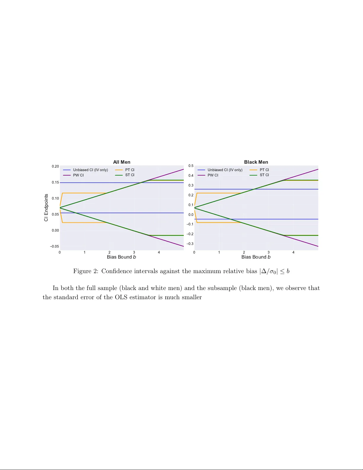
In tro ducing the b-v alue: com bining un biased and biased estimators from a sensitivit y analysis p ersp ectiv e Zhexiao Lin ∗ , P eter J. Bick el † , and P eng Ding ‡ F ebruary 19, 2026 Abstract In empirical researc h, when we ha ve m ultiple estimators for the same parameter of in terest, a cen tral question arises: how do w e combine unbiased but less precise estimators with biased but more precise ones to improv e the inference? Under this setting, the p oin t estimation prob- lem has attracted considerable atten tion. In this pap er, w e fo cus on a less studied inference question: ho w can we conduct v alid statistical inference in suc h settings with unknown bias? W e prop ose a strategy to combine unbiased and biased estimators from a sensitivity analysis p erspective. W e deriv e a sequence of conﬁdence interv als indexed by the magnitude of the bias, whic h enable researc hers to assess how conclusions v ary with the bias levels. Importantly , we in tro duce the notion of the b-v alue, a critical v alue of the unkno wn maxim um relative bias at whic h com bining estimators does not yield a signiﬁcant result. W e apply this strategy to three canonical com bined estimators: the precision-w eighted estimator, the pretest estimator, and the soft-thresholding estimator. F or each estimator, w e c haracterize the sequence of conﬁdence in- terv als and determine the bias threshold at whic h the conclusion changes. Based on the theory , w e recommend rep orting the b-v alue based on the soft-thresholding estimator and its asso ciated conﬁdence interv als, wh ic h are robust to unknown bias and achiev e the lo west worst-case risk among the alternatives. Keyw ords : data fusion, data in tegration, pretest, shrink age estimator, soft-thresholding. 1 In tro duction In empirical researc h, it is common for researchers to employ diﬀerent metho ds to estimate the same parameter of interest. These diﬀerences ma y arise from the use of distinct datasets or from imp osing diﬀeren t mo del assumptions on the same dataset. W e motiv ate our pap er with the following tw o examples of com bining estimators. Example 1.1. Randomized controlled trials (R CT s) are the gold standard for estimating treatment eﬀects due to their abilit y to eliminate unmeasured confounding. Ho wev er, R CT s often suﬀer from ∗ Departmen t of Statistics, Universit y of California, Berk eley , CA 94720, USA; e-mail: zhexiaolin@berkeley.edu † Departmen t of Statistics, Univ ersity of California, Berkeley , CA 94720, USA; e-mail: bickel@stat.berkeley.edu ‡ Departmen t of Statistics, Univ ersity of California, Berkeley , CA 94720, USA; e-mail: pengdingpku@berkeley.edu 1 limited sample sizes, as large-scale exp erimen ts can b e costly or infeasible. In con trast, observ ational data are more readily av ailable from the target population of interest. Ho wev er, estimates using observ ational data may b e biased in estimating treatment eﬀects due to unmeasured confounding, raising concerns ab out the internal v alidit y . See Brant ner et al. ( 2023 ) and Colnet et al. ( 2024 ) for recen t reviews on motiv ations and metho ds for combining R CT s and observ ational studies. Example 1.2. The ordinary least squares (OLS) estimator is biased in estimating the unknown parameters under the linear mo del when the error term is correlated with the regressor. In contrast, the instrumental v ariables (IV) estimator can provide un biased estimates for the parameters of in terest with a v alid instrumen tal v ariable that is uncorrelated with the error term but correlated with the regressor. Ho wev er, the IV estimator is usually muc h less precise than the OLS estimator, esp ecially when the IV is w eakly correlated with the regressor ( Bound et al. , 1995 ). In empirical studies, e.g., Angrist and Krueger ( 1991 ), researc hers often rep ort results from b oth OLS and IV estimators. Ho w to combine OLS and IV estimators is gaining increasing in terest ( Armstrong et al. , 2025 ). When the estimators are from diﬀeren t datasets, e.g., Example 1.1 , the estimators are inde- p enden t as long as the datasets are indep endent. When the estimators are from the same dataset but with diﬀeren t mo del assumptions, e.g., Example 1.2 , the estimators are dep enden t in general. Giv en access to multiple potentially dep enden t estimators, some unbiased but less precise and others biased but more precise, a natural question is: How can we combine the unbiased and p otentially biased estimators to improv e the inference with unknown bias? F rom the p oin t estimation p erspec- tiv e, this problem has b een extensiv ely studied ( Bic kel , 1984 ; Green and Strawderman , 1991 ; Giles and Giles , 1993 ; Chen et al. , 2015 ; A they et al. , 2020 ; de Chaisemartin and D’Haultfœuille , 2020 ; Rosenman et al. , 2023a ; Gao and Y ang , 2023 ; Y ang et al. , 2025 ). Man y metho ds hav e b een prop osed for constructing combined estimators that p erform w ell when the bias is small and ha ve b ounded risks when the bias is large. F rom the statistical inference p ersp ectiv e, this problem is less studied. In this pap er, w e answ er the follo wing question: ho w can w e conduct v alid statistical inference after com bining the estimators? This question has receiv ed considerably less atten tion. The primary diﬃculty lies in the imp os- sibilit y of characterizing the distribution of the combined estimator with unkno wn bias ( Armstrong et al. , 2025 ). Once the information ab out the bias is introduced, e.g., an upp er b ound on its mag- nitude, conﬁdence interv als for the parameter of interest b ecome p ossible. In the absence of suc h information, w e fo cus on the follo wing question: How c an we c onstruct a se quenc e of c onﬁdenc e intervals for the p ar ameter of inter est acr oss bias levels? The sequence of conﬁdence interv als provides a wa y to quantify how the level of bias impacts the uncertaint y in p oin t estimation. One imp ortant application of this sequence is in h yp othesis testing. Supp ose the n ull hypothesis is not rejected based on the unbiased but less precise estimator. No w consider a scenario where the statistical test based on the biased but more precise estimator 2 rejects the null hypothesis. If we hav e prior knowledge suggesting the bias is small, incorp orating the biased estimator ma y yield a more precise estimator to reject the n ull hypothesis. In suc h cases, the sequence of conﬁdence in terv als enables us to address the follo wing question: How lar ge must the bias b e to change the c onclusion of a hyp othesis test—fr om r eje ction to non-r eje ction? The idea of constructing the sequence of conﬁdence in terv als and examining how conclusions c hange as the assumed level of bias v aries is related to sensitivity analysis in causal inference with unmeasured confounding, e.g., Cornﬁeld et al. ( 1959 ); Rosen baum and Rubin ( 1983 ); V anderW eele and Ding ( 2017 ). In observ ational studies, sensitivity analysis assesses how the causal conclusions c hange with resp ect to diﬀerent degrees of unmeasured confounding b y v arying the sensitivity pa- rameter ( Rosenbaum , 2002 ; Ding and V anderW eele , 2016 ). Our prop osed framework has a similar ﬂa vor: b y indexing inference results o v er a con tinuum of bias levels, w e can assess the robustness of statistical inference. W e formalize tw o statistical inference questions, conﬁdence in terv al and hypothesis testing, in the con text of combining unbiased and biased estimators. Under regularit y conditions, the estimators satisfy a join t central limit theorem. Consequen tly , w e presen t our formulation in a ﬁnite-sample Gaussian setting, assuming exact normality for both the unbiased and biased estimators. This reduction to a Gaussian mo del is motiv ated by Le Cam’s classical asymptotic argument ( Le Cam , 1956 ), and b ecause of this, our Gaussian formulation should b e view ed as an asymptotic idealization rather than a restrictiv e ﬁnite-sample assumption. W e dev elop a general framework that applies to an y p oin t estimator formed by combining such estimators. Within this framew ork, w e construct a sequence of conﬁdence interv als indexed by the bias level, and importantly , w e in tro duce the notion of the b-v alue, a critical v alue of the unkno wn maximum relativ e bias at whic h com bining estimators do es not yield a signiﬁcant result. W e examine three canonical com bined estimators: the precision-w eighted estimator, the pretest estimator, and the soft-thresholding estimator. F or eac h estimator, we derive either analytically or n umerically the sequence of conﬁdence interv als and the b-v alue. Among the three, we advocate for the soft-thresholding estimator, as it oﬀers robustness to unkno wn bias compared with the precision- w eighted estimator, and exhibits low er worst-case risk and more desirable prop erties for conﬁdence in terv al construction than the pretest estimator. W e provide a Python pac k age for the prop osed metho ds, av ailable at https://github.com/zhexiaolin/b- value . Notation. F or a vector a = ( a 1 , . . . , a d ) ⊤ ∈ R d , let ∥ a ∥ 1 = P d i =1 | a i | , ∥ a ∥ 2 = ( P d i =1 a 2 i ) 1 / 2 , and | a | = ( | a 1 | , . . . , | a d | ) ⊤ . F or v ectors a = ( a 1 , . . . , a d ) ⊤ and b = ( b 1 , . . . , b d ) ⊤ , let a ⊙ b = ( a 1 b 1 , . . . , a d b d ) ⊤ b e the Hadamard (elemen t-wise) product, and a ≤ b denote a i ≤ b i for all i = 1 , 2 , . . . , d . F or a scalar b ∈ R and a set A ⊂ R , we write b − A = { b − a : a ∈ A } , which extends naturally to vectors and sets in R d . W e use Φ( · ) and ϕ ( · ) to denote the cum ulativ e distribution function and densit y function of the standard normal distribution, resp ectiv ely . W e use ϕ µ , Σ ( · ) to denote the densit y function of the multiv ariate normal distribution with mean µ and cov ariance matrix Σ . W e use Ψ d ( · ; λ ) to denote the cum ulativ e distribution function of the noncen tral c hi- 3 squared distribution with noncentralit y parameter λ and degrees of freedom d . W e use c α to denote the (1 − α ) upp er quantile of the standard normal distribution. 2 Problem setup and a review of p oin t estimation 2.1 Problem Setup W e consider the follo wing setting: Assumption 2.1. Supp ose we observe two indep endent r andom variables: one unbiase d estimator b τ 0 ∼ N ( τ , σ 2 0 ) and one biase d estimator b τ 1 ∼ N ( τ + ∆ , σ 2 1 ) . Her e, τ ∈ R is the unknown p ar ameter of inter est. W e assume that σ 2 0 and σ 2 1 ar e known, wher e as ∆ is unknown. In practice, b oth the un biased and biased estimators for the same parameter of in terest are constructed from data. Under regularit y conditions, these estimators are join tly asymptotically normal with an unknown co v ariance matrix. As long as this cov ariance matrix can b e consistently estimated, the problem of combining estimators reduces to an exact normalit y framework under Le Cam’s asymptotic framework ( Le Cam , 1956 ). Le Cam ( 1956 ) show ed that a wide class of estima- tors and test statistics can b e appro ximated in large samples b y Gaussian exp erimen ts with known co v ariances. Within this framew ork, w e treat the estimators as arising from Gaussian exp erimen ts in whic h the v ariances are replaced by their consistent estimates, and the v alidity of the inference pro cedures is preserved asymptotically . F or this reason, w e present our analysis in the exact nor- malit y setting. Nevertheless, our results represen t the asymptotic limits of a broad class of more general and practically relev an t inference problems. The analysis can b e generalized to dep enden t (Section 3.5 ), m ultiv ariate (Section 4 ) and m ultiple estimators (Section 5 ) cases. Let γ = σ 2 0 /σ 2 1 b e the v ariance ratio b et ween b τ 0 and b τ 1 . In general, the unbiased estimator is less precise but the biased estimator is more precise. Therefore, we fo cus on the regime in whic h σ 2 0 is large and σ 2 1 is small, whic h indicates that γ is large. Under Assumption 2.1 , w e address the following central question: How c an we c onstruct a se quenc e of two-side d c onﬁdenc e intervals for τ acr oss diﬀer ent levels of bias ( ∆ )? W e fo cus on constructing tw o-sided symmetric conﬁdence in terv als centered at presp eciﬁed p oin t estimators. In other w ords, we do not let the p oint estimator itself depend on the bias lev el ∆ . An alternativ e approach would be to use a bias-dep enden t p oin t estimator, where the estimator incorp orates ∆ . W e will discuss the adv antages of using prespeciﬁed p oin t estimators later in App endix A.3 . Since b τ 0 is an un biased estimator of τ , one natural approac h is to construct a conﬁdence in terv al based solely on b τ 0 , which is inv ariant to the bias ∆ . Giv en a signiﬁcance level ζ ∈ (0 , 1) , w e can construct a standard t wo-sided conﬁdence interv al [ b τ 0 − σ 0 c ζ / 2 , b τ 0 + σ 0 c ζ / 2 ] , 4 where c ζ / 2 is the (1 − ζ / 2) upp er quantile of the standard normal distribution. While b eing v alid regardless of the bias ∆ , this conﬁdence interv al may b e to o wide when b τ 0 is not precise, whose length 2 σ 0 c ζ / 2 scales prop ortionally with σ 0 . As we hav e access to the additional biased but more precise estimator b τ 1 , a natural question arises: can we shorten the conﬁdence in terv al by incorp orating information from b τ 1 ? This motiv ates us to combine the tw o estimators b τ 0 and b τ 1 to construct a t wo-sided conﬁdence in terv al with shorter length. Consider a generic combined estimator b τ = b τ ( b τ 0 , b τ 1 , σ 2 0 , σ 2 1 ) of τ , whic h depends only on observed data ( b τ 0 , b τ 1 ) and kno wn v ariances ( σ 2 0 , σ 2 1 ) , but not on the unkno wn bias ∆ . If ∆ were known, constructing an exact tw o-sided conﬁdence interv al w ould b e straigh tforward, as the distributions of b oth estimators are known, which lead to kno wn distribution of b τ . How ev er, since ∆ is unknown, the exact conﬁdence interv al dep ends on the magnitude of ∆ . T o analyze the problem, w e imp ose b ounds on the bias ∆ and construct t wo-sided conﬁdence in terv als for diﬀeren t lev els of bias. W e assume that | ∆ /σ 0 | ≤ b for some b ≥ 0 , and study ho w the conﬁdence in terv al based on b τ c hanges as a function of the bias b ound b . Here we fo cus on the relativ e bias ∆ /σ 0 instead of the absolute bias ∆ to ensure that the parameterization is inv ariant to the scale of the estimators. F or a given b , w e aim to construct a tw o-sided conﬁdence interv al that ac hieves correct cov erage uniformly o ver all ∆ satisfying | ∆ /σ 0 | ≤ b . W e thus deﬁne the conﬁdence in terv al b elo w. Deﬁnition 2.1. Giv en a signiﬁcance level ζ ∈ (0 , 1) and a maxim um relative bias b ≥ 0 , we w ant to construct an in terv al I ( b, ζ ) = I ( b, ζ , b τ 0 , b τ 1 , σ 2 0 , σ 2 1 ) suc h that inf ∆: | ∆ /σ 0 |≤ b P ∆ ( τ ∈ b τ − I ( b, ζ )) = inf ∆: | ∆ /σ 0 |≤ b P ∆ ( b τ − τ ∈ I ( b, ζ )) ≥ 1 − ζ , (2.1) where P ∆ explicitly denotes the dep endence of the distribution of b τ on ∆ . The conﬁdence interv al for τ based on b τ is then given by b τ − I ( b, ζ ) . W e next imp ose tw o natural monotonicit y conditions on the interv al I ( b, ζ ) b elow. Assumption 2.2. W e assume: 1. F or ﬁxe d ( b τ 0 , b τ 1 , σ 2 0 , σ 2 1 ) and ζ , we have I ( b, ζ ) ⊂ I ( b ′ , ζ ) whenever b ≤ b ′ . 2. F or ﬁxe d ( b τ 0 , b τ 1 , σ 2 0 , σ 2 1 ) and b , we have I ( b, ζ ) ⊂ I ( b, ζ ′ ) whenever ζ ≥ ζ ′ . The ﬁrst condition in Assumption 2.2 requires that as we allo w greater bias in b τ 1 , the conﬁdence in terv al b ecomes wider and contains the previous interv als. The second condition in Assumption 2.2 requires that to guaran tee higher co verage rate, the conﬁdence in terv al m ust widen. A common class of in terv als satisfying b oth conditions is the class of symmetric ﬁxed-length centered in terv als, whose length do es not dep end on ( b τ 0 , b τ 1 ) , i.e., I ( b, ζ ) = [ − c ( b, ζ , σ 2 0 , σ 2 1 ) , c ( b, ζ , σ 2 0 , σ 2 1 )] for some c ( b, ζ , σ 2 0 , σ 2 1 ) ≥ 0 dep ending only on b , ζ , σ 2 0 , and σ 2 1 . In this case, the conﬁdence interv al b τ − I ( b, ζ ) in Deﬁnition 2.1 is giv en by [ b τ − c ( b, ζ , σ 2 0 , σ 2 1 ) , b τ + c ( b, ζ , σ 2 0 , σ 2 1 )] . 5 Therefore, for giv en ( b τ 0 , b τ 1 , σ 2 0 , σ 2 1 ) and ζ , we can regard the conﬁdence in terv al b τ − I ( b, ζ ) in Deﬁnition 2.1 as a function of the bias b ound b . Th us, to address the central question of constructing a sequence of t w o-sided conﬁdence in terv als for τ across diﬀeren t lev els of bias, we compute this conﬁdence in terv al for a range of v alues of b : { b τ − I ( b, ζ ) } b ≥ 0 . Once we construct the sequence of conﬁdence in terv als, a natural application is hypothesis testing ab out the parameter τ . W e fo cus on the t wo-sided test: H 0 : τ = 0 v ersus H 1 : τ  = 0 . (2.2) W e generalize the discussion to one-sided tests, suc h as testing τ = 0 v ersus τ > 0 or testing τ ≤ 0 v ersus τ > 0 , in Section A.2 . It is straigh tforward to extend the tw o-sided test to h yp otheses of the form τ = τ ∗ v ersus τ  = τ ∗ for any giv en τ ∗ ∈ R . A common practice for the tw o-sided test in volv es constructing conﬁdence interv als for τ and chec king whether the n ull v alue 0 lies within these in terv als. Under Assumption 2.2 , the width of the conﬁdence in terv al increases with the bias b ound b . This leads to a central question when using the combined estimator b τ with the conﬁdence interv al b τ − I ( b, ζ ) : How lar ge must the bias b ound b b e to change the c onclusion of the hyp othesis test ( 2.2 ) ? By the monotonicity of I ( b, ζ ) in b (holding ( b τ 0 , b τ 1 ) and ζ ﬁxed) from Assumption 2.2 , w e deﬁne the limiting interv al as I ( ∞ , ζ ) = lim b →∞ I ( b, ζ ) . Then there ma y exist a critical v alue of b at whic h the conﬁdence in terv al b τ − I ( b, ζ ) contains the null v alue tested in ( 2.2 ). W e fo cus on cases where the critical v alue exists. Sp eciﬁcally , we consider the case when 0 / ∈ b τ − I (0 , ζ ) but 0 ∈ b τ − I ( ∞ , ζ ) . In this scenario, w e deﬁne the b-v alue b elo w. Deﬁnition 2.2. Deﬁne the b-v alue as the critical v alue b ∗ of testing τ = 0 versus τ  = 0 : b ∗ ( ζ ) = b ∗ ( ζ , b τ 0 , b τ 1 , σ 2 0 , σ 2 1 ) = inf { b ≥ 0 : 0 ∈ b τ − I ( b, ζ ) } . (2.3) By the monotonicity conditions in Assumption 2.2 , we hav e 0 / ∈ b τ − I ( b, ζ ) for 0 ≤ b < b ∗ and 0 ∈ b τ − I ( b, ζ ) for b > b ∗ . Th us, we reject the null h yp othesis τ = 0 when b < b ∗ and fail to reject it for b > b ∗ . The b-v alue b ∗ th us represents the maxim um relative bias b ey ond whic h the null h yp othesis can no longer be rejected. W e prop ose to rep ort b ∗ deﬁned in ( 2.3 ) for giv en estimators ( b τ 0 , b τ 1 ) and signiﬁcance lev el ζ . Compared with the sensitivit y analysis literature, the bias b ound b in our framework plays a role analogous to the sensitivit y parameter. The corresp onding conﬁdence interv al b τ − I ( b, ζ ) serves as a sensitivity curve, illustrating how inference changes as the bias v aries. In this context, the b-v alue b ∗ serv es a role similar to key robustness metrics in prior work: it parallels the design sensitivity b y Rosenbaum ( 2004 ), the E-v alue b y V anderW eele and Ding ( 2017 ), and the robustness v alue by Cinelli and Hazlett ( 2020 ). The b-v alue b ∗ pro vides a criterion for comparing comp eting strategies of conﬁdence in terv al construction. Diﬀeren t c hoices of the com bined estimator b τ and diﬀerent formulations of I ( b, ζ ) can lead to diﬀerent v alues of b ∗ . W e prefer pro cedures that yield a larger b-v alue b ∗ , since this indicates 6 that the resulting conﬁdence interv al is more robust to p otential bias in the biased estimator. This role of b ∗ is analogous to that use of the design sensitivity in Rosen baum ( 2004 ), where it serves as a criterion for comparing diﬀeren t test statistics and matched designs in observ ational studies. Remark 2.1. Besides the scenario of primary interest: 0 / ∈ b τ − I (0 , ζ ) and 0 ∈ b τ − I ( ∞ , ζ ) , tw o other less in teresting scenarios may occur. First, if 0 ∈ b τ − I (0 , ζ ) , then 0 ∈ b τ − I ( b, ζ ) for all b ≥ 0 , and w e alw ays fail to reject the null hypothesis regardless of the bias magnitude. Second, if 0 / ∈ b τ − I ( ∞ , ζ ) , then 0 / ∈ b τ − I ( b, ζ ) for all b ≥ 0 , and we alw a ys reject the null h yp othesis regardless of the bias magnitude. In these tw o scenarios, com bining the estimators or not do es not c hange the statistical result qualitativ ely . Therefore, w e ignore them in our discussion. Dep ending on the choice of b τ and construction of I ( b, ζ ) , not all three scenarios may arise. W e fo cus on the case when the b-v alue b ∗ deﬁned in ( 2.3 ) is in the in terv al (0 , ∞ ) . 2.2 P oin t estimation: a review Before diving in to the details of the method for constructing conﬁdence in terv als and obtaining the b-v alue, we ﬁrst review the existing approaches to p oin t estimation. Sp eciﬁcally , we review three p oin t estimators: the precision-weigh ted estimator, the pretest estimator, and the soft-thresholding estimator. First, w e recall the precision-weigh ted estimator: b τ PW := σ 2 1 σ 2 0 + σ 2 1 b τ 0 + σ 2 0 σ 2 0 + σ 2 1 b τ 1 = b τ 0 + σ 2 0 σ 2 0 + σ 2 1 ( b τ 1 − b τ 0 ) = b τ 0 + γ 1 + γ ( b τ 1 − b τ 0 ) . When ∆ is known to b e 0, the precision-weigh ted estimator is the maximum likelihoo d estimator and b est linear un biased estimator of τ . Moreov er, b y the classical Le Cam asymptotic decision theory ( Le Cam , 1956 ) and classical results for the Gaussian shift mo del, it is asymptotically admissible and minimax under L 2 risk in general, i.e., E[( b τ − τ ) 2 ] , among all regular estimators under standard regularit y conditions. Ho wev er, b τ PW is not robust to bias: its risk is large when | ∆ | is large. This motiv ates us to consider a combined estimator that p erforms nearly as well as b τ PW when the bias is small, and is robust to unknown bias ∆ , ensuring that the w orst-case risk sup ∆ ∈ R E ∆ [( b τ − τ ) 2 ] remains b ounded. This motiv ates the following t w o estimators. Second, we recall the pretest estimator, which in volv es incorp orating a pretest for ∆ = 0 versus ∆  = 0 , a pro cedure that is commonly used ( Bancroft , 1944 ; W allace , 1977 ; Bancroft and Han , 1977 ; Giles and Giles , 1993 ). Under ∆ = 0 , given the indep endence b et ween b τ 1 and b τ 0 , their diﬀerence follo ws: b τ 1 − b τ 0 ∼ N (0 , σ 2 ) , where σ 2 = σ 2 0 + σ 2 1 . F or a ﬁxed signiﬁcance level α ∈ (0 , 1) , we consider the test statistic ( b τ 1 − b τ 0 ) /σ . Let A = {| b τ 1 − b τ 0 | ≤ σ c α/ 2 } denote the even t that the pretest fails to reject the null hypothesis ( ∆ = 0 ). If the pretest fails to reject the null hypothesis, i.e., | b τ 1 − b τ 0 | ≤ σ c α/ 2 , the pretest estimator uses the precision-weigh ted 7 estimator: b τ 0 + γ 1 + γ ( b τ 1 − b τ 0 ) . If the pretest rejects the n ull hypothesis, i.e., | b τ 1 − b τ 0 | > σ c α/ 2 , the pretest estimator emplo ys hard-thresholding by reverting to the unbiased estimator b τ 0 . Combining the t wo cases, the pretest estimator is: b τ PT = b τ 0 + γ 1 + γ ( b τ 1 − b τ 0 ) 1 ( A ) . Third, we recall the soft-thresholding estimator, whic h ensures con tinuit y at the pretest b ound- ary ( | b τ 1 − b τ 0 | = σ c α/ 2 ). If the pretest fails to reject the n ull hypothesis, the soft-thresholding estimator also uses the precision-weigh ted estimator. If the pretest rejects the null h yp othesis, the soft-thresholding estimator emplo ys soft-thresholding by: b τ 0 + γ 1 + γ σ c α/ 2 sign( b τ 1 − b τ 0 ) . Com bining the tw o cases, the soft-thresholding estimator is: b τ ST = b τ 0 + γ 1 + γ ( b τ 1 − b τ 0 ) 1 ( A ) + γ 1 + γ σ c α/ 2 sign( b τ 1 − b τ 0 ) 1 ( A c ) . While b τ PT reduces to b τ 0 with probability nearly one when the bias is large, the risk of b τ PT is m uch higher than that of b τ ST when the bias is mo derate. See Bick el ( 1983 ) and Armstrong et al. ( 2025 ) for a comparison of worst-case risk betw een b τ PT and b τ ST and the sup erior p erformance of b τ ST . In b oth b τ PT and b τ ST , the role of α is diﬀeren t from its usual in terpretation in hypothesis testing. Rather than a T yp e I error rate, α here acts as a tuning parameter that balances the bias and v ariance of the p oin t estimator. In this sense, α simply indexes a family of estimators, muc h like the p enalt y level in p enalized regression metho ds (e.g., the Lasso). Cho osing α optimally dep ends on ∆ , whic h is unknown in practice. In our empirical studies, w e set α = 0 . 05 as a default, following the standard con ven tion, and examine how the estimator’s p erformance v aries across diﬀeren t bias lev els. 3 Conﬁdence in terv als, h yp othesis testing, and the b-v alue Giv en the canonical p oin t estimators in troduced in Section 2.2 , we no w discuss the problem of constructing conﬁdence in terv als, h yp othesis testing, and the b-v alue. 3.1 Conﬁdence in terv al based on the precision-w eighted estimator As a warm-up, we use the precision-w eighted estimator b τ PW to construct the sequence of conﬁdence in terv als and to illustrate how the conﬁdence interv al c hanges with resp ect to b . Based on the theory b elo w, w e do not recommend using the precision-w eighted estimator and its corresp onding conﬁ- dence in terv als in practice. Under Assumption 2.1 , w e hav e b τ PW ∼ N ( τ + (1 + γ ) − 1 γ ∆ , (1 + γ ) − 1 σ 2 0 ) . The follo wing theorem pro vides the sequence of conﬁdence in terv als based on b τ PW dep ending on b . 8 Theorem 3.1. L et b L PW = b L PW ( b, ζ , γ ) ≥ 0 denote the solution to the e quation of L : Φ  L − γ √ 1 + γ b  − Φ  − L − γ √ 1 + γ b  = 1 − ζ . The b L PW always exists and is unique. The shortest length symmetric c enter e d c onﬁdenc e interval b ase d on b τ PW for τ satisfying ( 2.1 ) is given by [ b τ PW − b L PW (1 + γ ) − 1 / 2 σ 0 , b τ PW + b L PW (1 + γ ) − 1 / 2 σ 0 ] . The b L PW in Theorem 3.1 corresp onds to the (1 − ζ ) quantile of the folded normal distribution | N ( γ √ 1+ γ b, 1) | . This distribution also arises in the regression literature, where w orst-case bias is incorp orated into the construction of conﬁdence in terv als ( Armstrong et al. , 2020 , 2022 ). In the sp ecial case when b = 0 , we ha ve b L PW (0 , ζ , γ ) = c ζ / 2 , whic h yields the length of the conﬁdence interv al based on b τ PW to b e 2 c ζ / 2 (1 + γ ) − 1 / 2 σ 0 . F or comparison, recall that the length of the conﬁdence interv al solely based on b τ 0 is 2 c ζ / 2 σ 0 . Th us the length of the conﬁdence in terv al reduces by a factor of (1 + γ ) − 1 / 2 when using b τ PW instead of b τ 0 , whic h is small when γ is large, i.e., σ 2 0 is muc h larger than σ 2 1 . This indicates that b y using a more precise but p oten tially biased estimator, if w e ha ve prior kno wledge that the bias is small, then we can achiev e a muc h shorter conﬁdence in terv al. Giv en ζ and γ , the b L PW ( b, ζ , γ ) in Theorem 3.1 increases as b increases, and go es to inﬁnity as b → ∞ . Therefore, the precision-weigh ted estimator is not robust to unkno wn bias since the conﬁdence in terv al is not b ounded as the bias diverges. One in teresting observ ation is that b L PW dep ends on σ 2 0 and σ 2 1 only through γ , the v ariance ratio. This explains why the bias ∆ is scaled by σ 0 in the deﬁnition of b , and the conﬁdence in terv al is represen ted as [ b τ PW − b L PW (1 + γ ) − 1 / 2 σ 0 , b τ PW + b L PW (1 + γ ) − 1 / 2 σ 0 ] . 3.2 Conﬁdence in terv al based on the pretest estimator W e no w construct the conﬁdence in terv al for the pretest estimator b τ PT . In the following lemma, we presen t the distribution of b τ PT − τ . Lemma 3.1. L et Z 1 , Z 2 b e two indep endent standar d normal r andom variables. Then b τ PT − τ is distribute d as 1 √ 1 + γ σ 0 Z 1 + γ 1 + γ ∆ 1      Z 2 + r γ 1 + γ ∆ σ 0     ≤ c α/ 2  − r γ 1 + γ σ 0 Z 2 1      Z 2 + r γ 1 + γ ∆ σ 0     > c α/ 2  . By Lemma 3.1 , the distribution of b τ PT is a mixture of a normal distribution and a truncated normal distribution. W e deﬁne b L PT = b L PT ( b, ζ , σ 2 0 , σ 2 1 , α ) as the smallest length such that the conﬁdence in terv al [ b τ PT − b L PT (1 + γ ) − 1 / 2 σ 0 , b τ PT + b L PT (1 + γ ) − 1 / 2 σ 0 ] ac hieves correct co verage for all ∆ satisfying | ∆ /σ 0 | ≤ b , where w e choose the same scale as in Theorem 3.1 for comparison. By Deﬁnition 2.1 , w e can formulate b L PT as the optimization problem b L PT = b L PT ( b, ζ , σ 2 0 , σ 2 1 , α ) = inf  L ≥ 0 : inf ∆: | ∆ /σ 0 |≤ b P ∆ ( | b τ PT − τ | ≤ L (1 + γ ) − 1 / 2 σ 0 ) ≥ 1 − ζ  . (3.1) Ho wev er, b L PT generally does not admit a closed-form expression. Moreo ver, direct computation of b L PT based on ( 3.1 ) is computationally c hallenging since for eac h L ≥ 0 , the optimization problem 9 ( 3.1 ) inv olv es ﬁnding the inﬁm um of P ∆ ( | b τ PT − τ | ≤ L (1 + γ ) − 1 / 2 σ 0 ) ov er all ∆ satisfying | ∆ /σ 0 | ≤ b . Nev ertheless, we show that computing b L PT is tractable due to the follo wing theorem: Theorem 3.2. F or any L > 0 , P ∆ ( | b τ PT − τ | ≤ L (1 + γ ) − 1 / 2 σ 0 ) as a function of ∆ is symmetric ab out ∆ = 0 . Then b L PT = b L PT ( b, ζ , γ , α ) in ( 3.1 ) is the solution to the fol lowing e quation of L : min 0 ≤ t ≤ b P ∆ /σ 0 = t ( | b τ PT − τ | ≤ L (1 + γ ) − 1 / 2 σ 0 ) = 1 − ζ , wher e P ∆ /σ 0 = t ( | b τ PT − τ | ≤ L (1 + γ ) − 1 / 2 σ 0 ) = h Φ  c α/ 2 − r γ 1 + γ t  − Φ  − c α/ 2 − r γ 1 + γ t ih Φ  L − γ √ 1 + γ t  − Φ  − L − γ √ 1 + γ t i + Z − c α/ 2 − q γ 1+ γ t −∞ h Φ  L + √ γ u  − Φ  − L + √ γ u i ϕ ( u )d u + Z ∞ c α/ 2 − q γ 1+ γ t h Φ  L + √ γ u  − Φ  − L + √ γ u i ϕ ( u )d u. (3.2) [ b τ PT − b L PT (1 + γ ) − 1 / 2 σ 0 , b τ PT + b L PT (1 + γ ) − 1 / 2 σ 0 ] is the shortest length symmetric c enter e d c onﬁdenc e interval b ase d on b τ PT for τ satisfying ( 2.1 ) . W e hav e tw o main observ ations from Theorem 3.2 . First, for any L > 0 , the cov erage probabilit y P ∆ ( | b τ PT − τ | ≤ L (1 + γ ) − 1 / 2 σ 0 ) is symmetric about ∆ = 0 . As a result, instead of minimizing o ver all ∆ satisfying | ∆ /σ 0 | ≤ b as in ( 3.1 ), w e can restrict attention to the in terv al 0 ≤ ∆ /σ 0 ≤ b . Second, Theorem 3.2 pro vides an explicit expression for the cov erage probability P ∆ /σ 0 = t ( | b τ PT − τ | ≤ L (1 + γ ) − 1 / 2 σ 0 ) as a function of t and L . The ﬁrst term in ( 3.2 ) corresp onds to the ev en t that the pretest fails to reject the n ull hypothesis ( ∆ = 0 ), in whic h case b τ PT reduces to the precision- w eighted estimator. The second and third terms in ( 3.2 ) integrate ov er the regions where the pretest rejects the n ull hypothesis, in which case b τ PT reduces to the un biased estimator. Although the probability P ∆ /σ 0 = t ( | b τ PT − τ | ≤ L (1 + γ ) − 1 / 2 σ 0 ) admits a closed form for any L > 0 , the minimum of P ∆ /σ 0 = t ( | b τ PT − τ | ≤ L (1 + γ ) − 1 / 2 σ 0 ) ov er 0 ≤ t ≤ b is not explicitly av ailable in closed form, and thus must b e computed n umerically . Since the fu nction P ∆ /σ 0 = t ( | b τ PT − τ | ≤ L (1 + γ ) − 1 / 2 σ 0 ) is monotonically increasing with respect to L for L ≥ 0 , L ∗ PT can be computed n umerically using, for example, the bisection metho d, com bined with numerical computation of the minim um of P ∆ /σ 0 = t ( | b τ PT − τ | ≤ L (1 + γ ) − 1 / 2 σ 0 ) with resp ect to t for each candidate L . 3.3 Conﬁdence in terv al based on the soft-thresholding estimator W e now construct the conﬁdence interv al for the soft-thresholding estimator b τ ST . In the following lemma, w e present the distribution of b τ ST − τ . Lemma 3.2. L et Z 1 , Z 2 b e two indep endent standar d normal r andom variables. Then b τ ST − τ is distribute d as 1 √ 1 + γ σ 0 Z 1 + γ 1 + γ ∆ 1      Z 2 + r γ 1 + γ ∆ σ 0     ≤ c α/ 2  10 − r γ 1 + γ σ 0  Z 2 − c α/ 2 sign  Z 2 + r γ 1 + γ ∆ σ 0  1      Z 2 + r γ 1 + γ ∆ σ 0     > c α/ 2  . By Lemma 3.2 , the distribution of b τ ST is a mixture of a normal distribution and a truncated normal distribution. Supp ose | ∆ /σ 0 | ≤ b for some b > 0 . W e seek the shortest length b L ST = b L ST ( b, ζ , σ 2 0 , σ 2 1 , α ) suc h that the conﬁdence interv al [ b τ ST − b L ST (1 + γ ) − 1 / 2 σ 0 , b τ ST + b L ST (1 + γ ) − 1 / 2 σ 0 ] ac hieves correct cov erage uniformly ov er all ∆ with | ∆ /σ 0 | ≤ b . By Deﬁnition 2.1 , w e can formulate b L ST as the optimization problem: b L ST = inf  L ≥ 0 : inf ∆: | ∆ /σ 0 |≤ b P ∆ ( | b τ ST − τ | ≤ L (1 + γ ) − 1 / 2 σ 0 ) ≥ 1 − ζ  . (3.3) Ho wev er, b L ST generally do es not admit a closed-form expression. Moreov er, direct computation of b L ST based on ( 3.3 ) is computationally c hallenging since for each L ≥ 0 , the optimization problem ( 3.3 ) inv olv es ﬁnding the inﬁmum of P ∆ ( | b τ ST − τ | ≤ L (1 + γ ) − 1 / 2 σ 0 ) ov er all ∆ satisfying | ∆ /σ 0 | ≤ b . Nev ertheless, we show that b L ST can b e computed eﬃciently due to the follo wing theorem: Theorem 3.3. F or any L > 0 , P ∆ ( | b τ ST − τ | ≤ L (1 + γ ) − 1 / 2 σ 0 ) as a function of ∆ is symmetric ab out ∆ = 0 and monotonic al ly de cr e asing in | ∆ | . Then b L ST = b L ST ( b, ζ , γ , α ) in ( 3.3 ) is the solution to the fol lowing e quation of L : P ∆ /σ 0 = b ( | b τ ST − τ | ≤ L (1 + γ ) − 1 / 2 σ 0 ) = 1 − ζ , wher e P ∆ /σ 0 = t ( | b τ ST − τ | ≤ L (1 + γ ) − 1 / 2 σ 0 ) = h Φ  c α/ 2 − r γ 1 + γ t  − Φ  − c α/ 2 − r γ 1 + γ t ih Φ  L − γ √ 1 + γ t  − Φ  − L − γ √ 1 + γ t i + Z − c α/ 2 − q γ 1+ γ t −∞ h Φ  L + √ γ ( u + c α/ 2 )  − Φ  − L + √ γ ( u + c α/ 2 ) i ϕ ( u )d u + Z ∞ c α/ 2 − q γ 1+ γ t h Φ  L + √ γ ( u − c α/ 2 )  − Φ  − L + √ γ ( u − c α/ 2 ) i ϕ ( u )d u. (3.4) [ b τ ST − b L ST (1 + γ ) − 1 / 2 σ 0 , b τ ST + b L ST (1 + γ ) − 1 / 2 σ 0 ] is the shortest length symmetric c enter e d c onﬁdenc e interval b ase d on b τ ST for τ satisfying ( 2.1 ) . W e hav e tw o main observ ations from Theorem 3.3 . First, for any L > 0 , the cov erage probabilit y P ∆ ( | b τ ST − τ | ≤ L (1 + γ ) − 1 / 2 σ 0 ) is symmetric about ∆ = 0 , unlike the pretest estimator, monoton- ically decreasing in | ∆ | . This monotonicit y implies that the worst-case cov erage ov er the bias ∆ satisfying | ∆ /σ 0 | ≤ b as in ( 3.3 ) is alwa ys attained at the b oundary ∆ /σ 0 = b . The monotonicity of the cov erage probability P ∆ ( | b τ ST − τ | ≤ L (1 + γ ) − 1 / 2 σ 0 ) makes the computation of b L ST more eﬃcien t than that of b L PT . Second, Theorem 3.3 pro vides an explicit expression for the co verage probabilit y P ∆ /σ 0 = t ( | b τ ST − τ | ≤ L (1 + γ ) − 1 / 2 σ 0 ) as a function of t and L . The ﬁrst term in ( 3.4 ) corresp onds to the ev ent that the pretest fails to reject the n ull h yp othesis ( ∆ = 0 ), in whic h case b τ ST reduces to the precision-weigh ted estimator. The second and third terms in ( 3.4 ) integrate ov er 11 the regions where the pretest rejects the n ull hypothesis, in whic h case b τ ST reduces to the unbiased estimator with a constan t shift to ensure contin uit y at the pretest b oundary . Since P ∆ /σ 0 = b ( | b τ ST − τ | ≤ L (1 + γ ) − 1 / 2 σ 0 ) is monotonically increasing in L , b L ST can b e eﬃcien tly computed b y , for example, the bisection metho d. 3.4 Comparison of the p oin t estimators and conﬁdence in terv als Compared with b τ PW , b τ ST has b ounded w orst-case risk. The mean squared error of b τ ST remains b ounded regardless of the magnitude of the bias, whereas the mean squared error of b τ PW gro ws without b ound as the bias increases. Thus, b τ ST oﬀers a more balanced compromise b et ween eﬃciency and robustness: it retains eﬃciency comparable to b τ PW when the bias is small, yet its p erformance comparable to the un biased estimator when the bias is large. Compared with b τ PT , b τ ST enjo ys a desirable monotonicit y prop ert y: for any L > 0 , the probability P ∆ ( | b τ ST − τ | ≤ L ) decreases monotonically in | ∆ | (Theorem 3.3 ). This behavior parallels the result in Bick el ( 1983 ), which shows that the mean squared error of b τ ST increases monotonically in | ∆ | . This monotonicit y of b τ ST allo ws us to compute the conﬁdence interv al based on b τ ST more eﬃcien tly than b τ PT , as sho wn in Theorem 3.3 . Figure 1 compares the conﬁdence in terv als based on b τ ST , b τ PT , b τ PW , and the un biased estimator b τ 0 , as the bias bound b v aries. W e ﬁx σ 2 0 = 1 and b τ 0 = 1 . Let ζ = 0 . 05 and α = 0 . 05 . W e set b τ 1 = 2 and examine tw o scenarios: γ = 10 and γ = 100 . W e observe that when the bias b ound b is small, the conﬁdence in terv als based on b τ ST , b τ PT , and b τ PW are all shorter than that based on b τ 0 . Imp ortan tly , when the bias b ound b is small, the conﬁdence interv al based on b τ ST is shorter than b τ PT and is comparable to b τ PW . F urthermore, the conﬁdence in terv al length based on b τ ST remains b ounded, whereas that based on b τ PW gro ws without b ound as b increases. Therefore, b τ ST com bines the eﬃciency gains of precision-weigh ted metho ds when bias is small with robustness to large biases, making it a sup erior choice for inference in practice. 0 1 2 3 4 5 B i a s B o u n d b 2 0 2 4 6 CI Endpoints = 1 0 PW CI PT CI ST CI Unbiased CI 0 1 2 3 4 5 B i a s B o u n d b = 1 0 0 PW CI PT CI ST CI Unbiased CI Figure 1: Conﬁdence interv als against the maximum relativ e bias | ∆ /σ 0 | ≤ b 12 Remark 3.1 (Computing the b-v alue) . After plotting the estimators and their conﬁdence interv als as in Figure 1 , w e are ready to read the b-v alue for each estimator given the signiﬁcance level ζ . Since the sequence of conﬁdence interv als is diﬀeren t for diﬀerent estimators, the b-v alues are also diﬀeren t. Alternatively , we can also compute the b-v alue directly . A naiv e wa y is to use bisection metho d by the monotonicit y of the conﬁdence interv al, which inv olves computing the conﬁdence in terv al for each p ossible bias level b , and see whether the conﬁdence interv al contains the n ull v alue. Ho wev er, this pro cedure is computationally heavy since the computation of the conﬁdence interv al for a given b also inv olv es the bisection metho d when based on b τ PT and b τ ST . In App endix A.1 , w e prop ose a metho d to compute the b-v alue eﬃcien tly . 3.5 Generalization to the dep enden t case So far we assume independent un biased and biased estimators. In this section, w e generalize the ab o v e discussion to the case where b τ 0 and b τ 1 are jointly normal with kno wn correlation ρ . W e assume ρσ 1  = σ 0 , whic h trivially holds when σ 2 0 > σ 2 1 , or equiv alen tly γ > 1 . The k ey is to construct a biased estimator which is indep enden t of b τ 0 without losing information of b τ 1 . T o ac hieve that, w e deﬁne the reparametrization b τ ′ 1 = b τ 1 − ( ρσ 1 /σ 0 ) b τ 0 1 − ρσ 1 /σ 0 . (3.5) Then, b τ 0 and b τ ′ 1 are indep enden t, with b τ ′ 1 ∼ N ( τ + ∆ ′ , σ ′ 2 1 ) , where ∆ ′ = ∆ 1 − ρσ 1 /σ 0 , σ ′ 2 1 = (1 − ρ 2 ) σ 2 1 (1 − ρσ 1 /σ 0 ) 2 . Th us, the problem reduces to the indep enden t case considered ab o ve. In the reparametrization in ( 3.5 ), we need to kno w how the transformation rescales the bias and how to in terpret the relativ e bias. W e can compute the conﬁdence interv als and the b-v alue based on the reparametrization with indep enden t unbiased estimator b τ 0 and transformed biased estimator b τ ′ 1 . Let the conﬁdence in terv als and the b-v alue in the transformed problem b e b τ − I ′ ( b, ζ ) and b ∗ ′ , resp ectiv ely . Then the conﬁdence in terv als for the original problem are b τ − I ( b, ζ ) = b τ − I ′ ( b/ | 1 − ρσ 1 /σ 0 | , ζ ) and the b-v alue is b ∗ = | 1 − ρσ 1 /σ 0 | b ∗ ′ , respectively . W e relegate the tec hnical details to App endix A.4 . 4 Generalization to the m ultiv ariate case In this section, w e extend our framework to the m ultiv ariate case. Many applications inv olv e vector- v alued parameters rather than scalars. Consider tw o leading examples in causal inference. First, when a treatmen t has multiple lev els, the parameter of in terest is a vector of treatmen t eﬀects across those lev els. This setting also includes factorial designs, where researchers aim to estimate factorial eﬀects jointl y . Second, when the p opulation is partitioned in to subgroups, the fo cus is often on subgroup treatment eﬀects, yielding a v ector of conditional av erage treatmen t eﬀects indexed b y the subgroup v ariable ( Sch w artz et al. , 2026 ). Bey ond causal inference, similar issues arise in 13 regression settings. F or instance, when combining OLS and IV estimators, the target parameter can b e a vector of regression co eﬃcien ts. Therefore, generalization to the multiv ariate case is essential for applications where researc hers must make inferences about multiple parameters. 4.1 Setup W e consider the following m ultiv ariate setting: Assumption 4.1. Supp ose we observe two indep endent r andom ve ctors: one unbiase d estimator b τ 0 ∼ N ( τ , Σ 0 ) and one biase d estimator b τ 1 ∼ N ( τ + ∆ , Σ 1 ) . Her e τ ∈ R d is the unknown p ar ameter of inter est. W e assume that Σ 0 and Σ 1 ar e known but ∆ is unknown. As in the univ ariate case, w e presen t our analysis in the exact normality setting which asymp- totically captures the essential structure of inference as in W ald ( 1943 ) and Le Cam ( 1956 ). Our goal is to construct conﬁdence regions for τ at diﬀerent bias levels. Although w e assume indep en- den t un biased and biased estimators, the extension to the dependent case is straightforw ard; see Section 3.5 . Since b τ 0 is unbiased for τ , giv en signiﬁcance lev el ζ ∈ (0 , 1) , a natural conﬁdence region based solely on b τ 0 is the ellipsoid: { τ ∈ R d : ( b τ 0 − τ ) ⊤ Σ − 1 0 ( b τ 0 − τ ) ≤ χ 2 d, 1 − ζ } , (4.1) where χ 2 d, 1 − ζ is the (1 − ζ ) upp er quan tile of the chi-squared distribution with d degrees of freedom. Then w e consider combining the tw o estimators b τ 0 and b τ 1 , and we consider a generic combined estimator b τ = b τ ( b τ 0 , b τ 1 , Σ 0 , Σ 1 ) . W e assume that | [ Σ − 1 / 2 ∆ ] j | ≤ b j for some b j ≥ 0 for all j = 1 , 2 , . . . , d and study how the conﬁdence region c hanges with the maxim um relative bias v ector b = ( b 1 , b 2 , . . . , b d ) ⊤ . Here Σ = Σ ( Σ 0 , Σ 1 ) ∈ R d × d can b e any ﬁxed p ositiv e deﬁnite scaling matrix that dep ends on Σ 0 and Σ 1 , which corresp onds to σ 2 0 w e used in the univ ariate case. F or a given bias vector b , diﬀerent c hoices of Σ corresp ond to diﬀerent regions for the bias ∆ . In this pap er, w e do not discuss how to choose the scaling matrix Σ optimally . F or simplicity , one may take Σ = I d , where I d is the d × d iden tity matrix, or set Σ = Σ 0 as in the univ ariate case. Analogous to Deﬁnition 2.1 for the univ ariate case, the conﬁdence region is deﬁned b elo w. Deﬁnition 4.1. Given a signiﬁcance lev el ζ ∈ (0 , 1) and the maximum relativ e bias v ector b with b j ≥ 0 for all j = 1 , 2 , . . . , d , we seek a region I ( b , ζ ) = I ( b , ζ , b τ 0 , b τ 1 , Σ 0 , Σ 1 ) suc h that inf ∆ : | Σ − 1 / 2 ∆ |≤ b P ∆ ( τ ∈ b τ − I ( b , ζ )) = inf ∆ : | Σ − 1 / 2 ∆ |≤ b P ∆ ( b τ − τ ∈ I ( b , ζ )) ≥ 1 − ζ . (4.2) The conﬁdence region based on b τ is then given by b τ − I ( b , ζ ) . Then we introduce the monotonicit y conditions on the region I ( b , ζ ) b elo w, which generalizes Assumption 2.2 to the m ultiv ariate case. Assumption 4.2. W e assume: 1. F or ﬁxe d ( b τ 0 , b τ 1 , Σ 0 , Σ 1 ) and ζ , we have I ( b , ζ ) ⊂ I ( b ′ , ζ ) whenever b ≤ b ′ , i.e., b j ≤ b ′ j for al l j = 1 , 2 , . . . , d . 14 2. F or ﬁxe d ( b τ 0 , b τ 1 , Σ 0 , Σ 1 ) and b , we have I ( b , ζ ) ⊂ I ( b , ζ ′ ) whenever ζ ≥ ζ ′ . Assume I ( b , ζ ) satisﬁes the monotonicity conditions of Assumption 4.2 . A common family of suc h regions is ﬁxed-length cen tered ellipsoids: I ( b , ζ ) = { h ∈ R d : h ⊤ A − 1 h ≤ c ( b , ζ , Σ 0 , Σ 1 ) } with some constan t c ( b , ζ , Σ 0 , Σ 1 ) ≥ 0 and a p ositiv e deﬁnite matrix A . In this case, the conﬁdence region b τ − I ( b , ζ ) in Deﬁnition 4.1 is given by { τ ∈ R d : ( b τ − τ ) ⊤ A − 1 ( b τ − τ ) ≤ c ( b , ζ , Σ 0 , Σ 1 ) } . Remark 4.1. Unlik e the univ ariate case, the construction of conﬁdence regions in the m ultiv ariate setting is more complicated. First, in one dimension, the only conv ex conﬁdence set is an interv al, whereas in higher dimensions, there exists a wide v ariet y of admissible con vex conﬁdence regions. Although ellipsoidal regions enjo y optimality prop erties under sp eciﬁc conditions ( Stein , 1962 ; W ald , 1949 ), the appropriate geometry dep ends on the family of contrasts and the norm used to measure uncertain ty . Ellipsoidal regions based on the Mahalanobis distance ( Hotelling , 1931 ) arise naturally under the Gaussian mo del, but alternative geometries hav e b een studied in the literature ( T ukey , 1949 ; Sc heﬀé , 1953 ; Šidák , 1967 ). Second, the optimal choice of the cen ter of the conﬁdence region is not straigh tforward. F or d ≥ 3 , Stein’s phenomenon implies that recentering at shrink age esti- mators such as the James–Stein estimator can yield conﬁdence regions with smaller v olume while main taining nominal co v erage ( Stein , 1962 ; Hw ang and Casella , 1982 ; Berger , 1985 ). In this sec- tion we follo w one sp eciﬁc trac k: constructing ellipsoidal conﬁdence regions under the Mahalanobis distance, cen tered at presp eciﬁed estimators, in parallel with our discussion for the univ ariate case in Section 3 . W e do not fo cus on the optimalit y among all p ossible shap es or centers, but rather fo cus on this formulation for its analytical tractabilit y and interpret ability within our framew ork. Then w e deﬁne the multiv ariate b-v alue b elo w. Deﬁnition 4.2. Deﬁne the b-v alue as the critical boundary b ∗ of testing τ = 0 v ersus τ  = 0 as b ∗ ( ζ ) = b ∗ ( ζ , b τ 0 , b τ 1 , Σ 0 , Σ 1 ) = ∂ { b ≥ 0 : 0 ∈ b τ − I ( b , ζ ) } . (4.3) Deﬁnition 4.2 extends the univ ariate notion of the b-v alue (Deﬁnition 2.2 ) to the multiv ariate setting. In higher dimensions d > 1 , the set { b ≥ 0 : 0 ∈ b τ − I ( b , ζ ) } is a con vex region in the ﬁrst quadran t. The b-v alue is deﬁned as the b oundary of this region, ∂ { b ≥ 0 : 0 ∈ b τ − I ( b , ζ ) } , whic h is a ( d − 1) -dimensional surface, e.g., a curve when d = 2 , in the ﬁrst quadrant. When d = 1 , this b oundary reduces to the single left endp oin t inf { b ≥ 0 : 0 ∈ b τ − I ( b, ζ ) } , which is exactly Deﬁnition 2.2 . By the monotonicit y conditions in Assumption 4.2 , the geometry of this b oundary yields a natural decision rule: we reject the null hypothesis τ = 0 if the bias bound vector b lies to the left of the b-v alue surface, and fail to reject it if b lies on or to the righ t of the b-v alue surface. T o compute and visualize the multiv ariate b-v alue, w e can plot the estimators and their conﬁdence regions, and then w e are ready to read the b-v alue for each estimator giv en the signiﬁcance lev el ζ . 4.2 P oin t estimation First, w e recall the precision-weigh ted estimator deﬁned as b τ PW = ( Σ − 1 0 + Σ − 1 1 ) − 1 ( Σ − 1 0 b τ 0 + Σ − 1 1 b τ 1 ) = b τ 0 + ( Σ − 1 0 + Σ − 1 1 ) − 1 Σ − 1 1 ( b τ 1 − b τ 0 ) . 15 The precision-w eigh ted estimator is the maxim um lik eliho od estimator of τ if ∆ is kno wn to b e all zeros. Ho wev er, its risk is large when ∥ ∆ ∥ 2 is large. Th us, we seek a combined estimator that p erforms nearly as w ell as b τ PW when the bias is small, and is robust to unknown bias ∆ , ensuring that the maxim um risk sup ∆ ∈ R d E ∆ [ ∥ b τ PW − τ ∥ 2 2 ] remains bounded. T o dev elop estimators that p erform well under zero bias yet remain robust to unknown bias, v arious estimators ha ve b een prop osed in the empirical Bay es and shrink age estimation literature ( Berger , 1981 ; Bic kel , 1984 ; Green and Strawderman , 1991 ; Green et al. , 2005 ; Rosenman et al. , 2023a , b ). In this pap er, w e fo cus on the generic pretest estimator and the generic soft-thresholding estimator, as discussed b elo w. Second, we recall the pretest estimator, which in v olves incorporating a pretest for ∆ = 0 v ersus ∆  = 0 . Under ∆ = 0 , given the indep endence b et ween b τ 1 and b τ 0 , their diﬀerence follo ws: b τ 1 − b τ 0 ∼ N ( 0 , Σ 0 + Σ 1 ) . W e consider the test statistic ∥ ( Σ 0 + Σ 1 ) − 1 / 2 ( b τ 1 − b τ 0 ) ∥ 2 2 and the critical v alue q ≥ 0 . The critical v alue q here pla ys a similar role as the signiﬁcance lev el α in Section 2.2 . Let A = {∥ ( Σ 0 + Σ 1 ) − 1 / 2 ( b τ 1 − b τ 0 ) ∥ 2 2 ≤ q } denote the ev ent that the pretest fails to reject the n ull hypothesis ( ∆ = 0 ). If the pretest fails to reject the null hypothesis, i.e., ∥ ( Σ 0 + Σ 1 ) − 1 / 2 ( b τ 1 − b τ 0 ) ∥ 2 2 ≤ q , the pretest estimator uses the precision-w eighted estimator: b τ 0 + ( Σ − 1 0 + Σ − 1 1 ) − 1 Σ − 1 1 ( b τ 1 − b τ 0 ) . If the pretest rejects the null h yp othesis, i.e., ∥ ( Σ 0 + Σ 1 ) − 1 / 2 ( b τ 1 − b τ 0 ) ∥ 2 2 > q , the pretest estimator emplo ys hard-thresholding b y reverting to the un biased estimator b τ 0 . Combining the t wo cases, the pretest estimator is: b τ PT = b τ 0 + ( Σ − 1 0 + Σ − 1 1 ) − 1 Σ − 1 1 ( b τ 1 − b τ 0 ) 1 ( A ) . Third, we recall the soft-thresholding estimator, whic h ensures con tinuit y at the pretest b ound- ary ( ∥ ( Σ 0 + Σ 1 ) − 1 / 2 ( b τ 1 − b τ 0 ) ∥ 2 2 = q ). If the pretest fails to reject the n ull h yp othesis, the soft- thresholding estimator also uses the precision-weigh ted estimator. If the pretest rejects the n ull h yp othesis, the soft-thresholding estimator emplo ys soft-thresholding by: b τ 0 + h ∗ q ( ∥ ( Σ 0 + Σ 1 ) − 1 / 2 ( b τ 1 − b τ 0 ) ∥ 2 2 )( Σ − 1 0 + Σ − 1 1 ) − 1 Σ − 1 1 ( b τ 1 − b τ 0 ) , where h ∗ q ( · ) : [ q , ∞ ) → [0 , 1] is a non-increasing function with h ∗ q ( q ) = 1 . Com bining the tw o cases, the soft-thresholding estimator is: b τ ST = b τ 0 + h q ( ∥ ( Σ 0 + Σ 1 ) − 1 / 2 ( b τ 1 − b τ 0 ) ∥ 2 2 )( Σ − 1 0 + Σ − 1 1 ) − 1 Σ − 1 1 ( b τ 1 − b τ 0 ) , where h q ( · ) : [0 , ∞ ) → [0 , 1] is deﬁned as h q ( r ) = 1 (0 ≤ r ≤ q ) + h ∗ q ( r ) 1 ( r > q ) . Here b oth q and h ∗ q ( · ) can dep end on Σ 0 and Σ 1 . The generic soft-thresholding estimator b τ ST con tains man y classical estimators as sp ecial cases, suc h as the estimator studied in Berger ( 1981 , Theorem 3) and Bick el ( 1984 , Section 4), whic h generalizes the univ ariate soft-thresholding estimator b τ ST to the multiv ariate setting. W e provide a detailed discussion of the relationship betw een the generic soft-thresholding estimator and the 16 estimator in Berger ( 1981 ); Bick el ( 1984 ) in App endix A.5 . In this pap er, w e fo cus on general Σ 0 , Σ 1 , and h ∗ q ( · ) . 4.3 Conﬁdence in terv als First, w e construct the conﬁdence regions based on the precision-weigh ted estimator b τ PW . Under Assumption 4.1 , we hav e b τ PW ∼ N ( τ + ( Σ − 1 0 + Σ − 1 1 ) − 1 Σ − 1 1 ∆ , ( Σ − 1 0 + Σ − 1 1 ) − 1 ) . By using the ellipsoidal conﬁdence region under the Mahalanobis distance and the co v ariance matrix of b τ PW , we consider the conﬁdence region based on b τ PW with the follo wing form: { τ ∈ R d : ( b τ PW − τ ) ⊤ ( Σ − 1 0 + Σ − 1 1 )( b τ PW − τ ) ≤ M } , for some M ≥ 0 . The follo wing theorem explicitly c haracterizes the conﬁdence region based on b τ PW as a function of bias b ound b . Theorem 4.1. L et c M PW = c M PW ( b , ζ , Σ 0 , Σ 1 , Σ ) ≥ 0 b e the (1 − ζ ) upp er quantile of the nonc entr al chi-squar e d distribution with d de gr e es of fr e e dom and nonc entr ality p ar ameter sup s ∈{± 1 } d    ( Σ − 1 0 + Σ − 1 1 ) − 1 / 2 Σ − 1 1 Σ 1 / 2 b ⊙ s    2 2 . The c onﬁdenc e r e gion for τ satisfying ( 4.2 ) is given by { τ ∈ R d : ( b τ PW − τ ) ⊤ ( Σ − 1 0 + Σ − 1 1 )( b τ PW − τ ) ≤ c M PW } . Theorem 4.1 extends the univ ariate result in Theorem 3.1 to the multiv ariate setting. In the univ ariate case, taking Σ = σ 2 0 and b = b reduces the m ultiv ariate conﬁdence region in Theorem 4.1 exactly to the conﬁdence in terv al in Theorem 3.1 . In the univ ariate case, the bias constrain t { ∆ : | ∆ /σ 0 | ≤ b } has only tw o b oundary p oin ts, and the absolute bias of b τ PW is the same at b oth endp oin ts. By contrast, the multiv ariate bias constrain t { ∆ : | Σ − 1 / 2 ∆ | ≤ b } is a con vex h yp errectangle with 2 d v ertices, and the maximum L 2 norm of the bias of b τ PW ma y o ccur at an y of these vertices. Theorem 4.1 therefore characterizes the maximum p ossible bias of b τ PW o ver the en tire bias constraint. In the sp ecial case when b = 0 , we ha ve c M PW = χ 2 d, 1 − ζ . Compared with the ellipsoid conﬁdence region based on b τ 0 , the scaling matrix in the deﬁnition of ellipsoid conﬁdence region reduces from Σ − 1 0 to Σ − 1 0 + Σ − 1 1 = ( Σ − 1 1 Σ 0 + I d ) Σ − 1 0 , analogous to the eﬃciency gain in the univ ariate case, where Σ − 1 1 Σ 0 can b e regarded as the v ariance ratio γ in the univ ariate case. As b increases, c M PW increases, and go es to inﬁnity as b → ∞ . Second, w e construct the conﬁdence regions based on the generic pretest estimator b τ PT . Similar to the conﬁdence regions based on the precision-w eighted estimator, w e consider the conﬁdence regions based on b τ PT with the follo wing form: { τ ∈ R d : ( b τ PT − τ ) ⊤ ( Σ − 1 0 + Σ − 1 1 )( b τ PT − τ ) ≤ M } , for some M ≥ 0 . Here, we fo cus on the ellipsoid conﬁdence region deﬁned using the same scaling matrix, Σ − 1 0 + Σ − 1 1 , as that used in the precision-weigh ted estimator. This c hoice allo ws for a direct comparison with the conﬁdence region based on the precision-w eighted estimator through the upp er 17 b ound M in the conﬁdence region. T o ensure the conﬁdence regions satisfy Deﬁnition 4.1 , w e need to ﬁnd the minimal v alue c M PT = c M PT ( b , ζ , Σ 0 , Σ 1 , Σ ) suc h that the conﬁdence region { τ ∈ R d : ( b τ PT − τ ) ⊤ ( Σ − 1 0 + Σ − 1 1 )( b τ PT − τ ) ≤ c M PT } ac hieves correct cov erage for all ∆ satisfying | [ Σ − 1 / 2 ∆ ] j | ≤ b j for all j = 1 , 2 , . . . , d . W e can form ulate c M PT as the optimization problem c M PT = inf  M ≥ 0 : inf ∆ : | Σ − 1 / 2 ∆ |≤ b P ∆ (( b τ PT − τ ) ⊤ ( Σ − 1 0 + Σ − 1 1 )( b τ PT − τ ) ≤ M ) ≥ 1 − ζ  . W e show ho w to compute c M PT in the follo wing theorem. Theorem 4.2. c M PT is the solution to the e quation of M : inf ∆ : | Σ − 1 / 2 ∆ |≤ b P ∆ (( b τ PT − τ ) ⊤ ( Σ − 1 0 + Σ − 1 1 )( b τ PT − τ ) ≤ M ) = 1 − ζ , with an explicit form given by: P Σ − 1 / 2 ∆ = t  ( b τ PT − τ ) ⊤ ( Σ − 1 0 + Σ − 1 1 )( b τ PT − τ ) ≤ M  =Ψ d  M ;    ( Σ − 1 0 + Σ − 1 1 ) − 1 / 2 Σ − 1 1 Σ 1 / 2 t    2 2  Ψ d  q ;    ( Σ 0 + Σ 1 ) − 1 / 2 Σ 1 / 2 t    2 2  + Z ∥ u ∥ 2 2 >q Ψ d  M ;    ( Σ − 1 0 + Σ − 1 1 ) − 1 / 2 Σ − 1 1 [ Σ 1 / 2 t − ( Σ 0 + Σ 1 ) 1 / 2 u ]    2 2  ϕ ( Σ 0 + Σ 1 ) − 1 / 2 Σ 1 / 2 t , I d ( u ) d u . (4.4) Theorem 4.2 extends the univ ariate result in Theorem 3.2 to the multiv ariate setting. Theo- rem 4.2 provides an explicit expression for the cov erage probability P Σ − 1 / 2 ∆ = t (( b τ PT − τ ) ⊤ ( Σ − 1 0 + Σ − 1 1 )( b τ PT − τ ) ≤ M ) as a function of M and t . The ﬁrst term in ( 4.4 ) corresp onds to the ev ent that the pretest fails to reject the null h yp othesis ( ∆ = 0 ), in which case b τ PT reduces to the precision- w eighted estimator. The second term in ( 4.4 ) integrates ov er the regions where the pretest rejects the n ull hypothesis, in which case b τ PT reduces to the un biased estimator. Third, we construct the conﬁdence regions based on the generic soft-thresholding estimator b τ ST . Similar to the conﬁdence regions based on the precision-w eighted estimator, we consider the conﬁdence regions based on b τ ST with the follo wing form: { τ ∈ R d : ( b τ ST − τ ) ⊤ ( Σ − 1 0 + Σ − 1 1 )( b τ ST − τ ) ≤ M } , for some M ≥ 0 . T o ensure the conﬁdence regions satisfy Deﬁnition 4.1 , we need to ﬁnd the minimal v alue c M ST = c M ST ( b , ζ , Σ 0 , Σ 1 , Σ ) suc h that the conﬁdence region { τ ∈ R d : ( b τ ST − τ ) ⊤ ( Σ − 1 0 + Σ − 1 1 )( b τ ST − τ ) ≤ c M ST } ac hieves correct cov erage for all ∆ satisfying | [ Σ − 1 / 2 ∆ ] j | ≤ b j for all j = 1 , 2 , . . . , d . W e can form ulate c M ST as the optimization problem c M ST = inf  M ≥ 0 : inf ∆ : | Σ − 1 / 2 ∆ |≤ b P ∆ (( b τ ST − τ ) ⊤ ( Σ − 1 0 + Σ − 1 1 )( b τ ST − τ ) ≤ M ) ≥ 1 − ζ  . W e show that c M ST can b e computed eﬃciently in the follo wing theorem. 18 Theorem 4.3. c M ST is the solution to the e quation of M : inf ∆ : Σ − 1 / 2 ∆ = b ⊙ s , s ∈{− 1 , 1 } d P ∆ (( b τ ST − τ ) ⊤ ( Σ − 1 0 + Σ − 1 1 )( b τ ST − τ ) ≤ M ) = 1 − ζ , with an explicit form given by: P Σ − 1 / 2 ∆ = t  ( b τ ST − τ ) ⊤ ( Σ − 1 0 + Σ − 1 1 )( b τ ST − τ ) ≤ M  =Ψ d  M ;    ( Σ − 1 0 + Σ − 1 1 ) − 1 / 2 Σ − 1 1 Σ 1 / 2 t    2 2  Ψ d  q ;    ( Σ 0 + Σ 1 ) − 1 / 2 Σ 1 / 2 t    2 2  + Z ∥ u ∥ 2 2 >q Ψ d  M ;    ( Σ − 1 0 + Σ − 1 1 ) − 1 / 2 Σ − 1 1 [ Σ 1 / 2 t − (1 − h ∗ q ( ∥ u ∥ 2 2 ))( Σ 0 + Σ 1 ) 1 / 2 u ]    2 2  ϕ ( Σ 0 + Σ 1 ) − 1 / 2 Σ 1 / 2 t , I d ( u ) d u . (4.5) Theorem 4.3 extends the univ ariate result in Theorem 3.3 to the multiv ariate setting. Theo- rem 4.3 provides an explicit expression for the cov erage probabilit y P Σ − 1 / 2 ∆ = t (( b τ ST − τ ) ⊤ ( Σ − 1 0 + Σ − 1 1 )( b τ ST − τ ) ≤ M ) as a function of M and t . The ﬁrst term in ( 4.5 ) corresp onds to the even t that the pretest fails to reject the null hypothesis ( ∆ = 0 ), in which case b τ ST reduces to the precision- w eighted estimator. The second term in ( 4.5 ) integrates ov er the regions where the pretest rejects the n ull hypothesis, in whic h case b τ ST reduces to the un biased estimator with a nonconstan t shift to ensure con tinuit y at the pretest b oundary . As in the univ ariate case, the monotonicity of the co verage probability makes the computation of c M ST more eﬃcien t than that of c M PT . F or an y M > 0 , the cov erage probability is minimized at the boundary of the bias region, namely at the v ertices ∆ satisfying Σ − 1 / 2 ∆ = b ⊙ s for some s ∈ {− 1 , 1 } d . Using Theorems 4.1 – 4.3 , we can construct conﬁdence regions based on b τ PW , b τ PT , and b τ ST for v arious bias b ounds b and signiﬁcance levels ζ . 5 Generalization to multiple estimators In this section, w e extend our framework to the multiple estimators setting. In empirical researc h, analysts often face the c hallenge of in tegrating evidence from datasets of heterogeneous qualit y . A leading example in causal inference is to combine an RCT with multiple observ ational studies. While the RCT provides un biased but often noisy estimates, observ ational studies can oﬀer m uch larger sample sizes but are sub ject to hidden bias due to unmeasured confounding. Bey ond causal inference, similar problems o ccur when synthesizing results from multiple registries, surv eys, or administrativ e databases, where no single source is suﬃcient on its o wn. W e presen t our theory b elo w. 5.1 Setup W e consider the follo wing multiple estimators setting with one unbiased estimator and K p oten tially biased estimators. W e can generalize to the case where there are multiple un biased estimators estimating the same parameter. In that case, w e can ﬁrst combine all the unbiased estimators into 19 a single unbiased estimator with smaller v ariance using the precision-w eighted estimator. Then w e can apply our current framew ork to combine this aggregated unbiased estimator with m ultiple biased estimators. Assumption 5.1. Supp ose we observe K + 1 indep endent r andom variables: one unbiase d estimator b τ 0 ∼ N ( τ , σ 2 0 ) and K p otential ly biase d estimators b τ j ∼ N ( τ + ∆ j , σ 2 j ) for j = 1 , . . . , K . Her e τ ∈ R is the unknown p ar ameter of inter est. W e assume that σ 2 0 , σ 2 1 , . . . , σ 2 K ar e known, wher e as ∆ 1 , . . . , ∆ K ar e unknown. Let γ j = σ 2 0 /σ 2 j b e the v ariance ratio b etw een the unbiased estimator and the j -th biased estimator. Let γ = ( γ 1 , . . . , γ K ) ⊤ b e the vector of v ariance ratios. W e consider a generic com bined estimator b τ = b τ ( b τ 0 , b τ 1 , . . . , b τ K , σ 2 0 , σ 2 1 , . . . , σ 2 K ) . W e assume that | ∆ j /σ 0 | ≤ b j for some b j > 0 for all j = 1 , . . . , K and study how the conﬁdence interv al changes with the maximum relativ e bias vector b = ( b 1 , . . . , b K ) . Let ∆ = (∆ 1 , . . . , ∆ K ) b e the vector of unknown biases. Analogous to Deﬁnition 2.1 for the univ ariate case, the conﬁdence in terv al is deﬁned b elo w. Deﬁnition 5.1. Given a signiﬁcance lev el ζ ∈ (0 , 1) and the maximum relativ e bias v ector b with b j ≥ 0 for all j = 1 , . . . , K , w e w ant to construct an in terv al I ( b , ζ ) = I ( b , ζ , b τ 0 , b τ 1 , . . . , b τ K , σ 2 0 , σ 2 1 , . . . , σ 2 K ) suc h that inf ∆ : | ∆ /σ 0 |≤ b P ∆ ( τ ∈ b τ − I ( b , ζ )) = inf ∆ : | ∆ /σ 0 |≤ b P ∆ ( b τ − τ ∈ I ( b , ζ )) ≥ 1 − ζ , (5.1) The conﬁdence in terv al for τ based on b τ is then given by b τ − I ( b , ζ ) . Then w e in tro duce the monotonicity conditions on the interv al I ( b , ζ ) b elow, which generalizes Assumption 2.2 to the m ultiple estimators setting. Assumption 5.2. W e assume: 1. F or ﬁxe d ( b τ 0 , b τ 1 , . . . , b τ K , σ 2 0 , σ 2 1 , . . . , σ 2 K ) and ζ , we have I ( b , ζ ) ⊂ I ( b ′ , ζ ) whenever b ≤ b ′ , i.e., b j ≤ b ′ j for al l j = 1 , . . . , K . 2. F or ﬁxe d ( b τ 0 , b τ 1 , . . . , b τ K , σ 2 0 , σ 2 1 , . . . , σ 2 K ) and b , we have I ( b , ζ ) ⊂ I ( b , ζ ′ ) whenever ζ ≥ ζ ′ . Assume I ( b , ζ ) satisﬁes the monotonicity conditions of Assumption 5.2 . A common family of suc h in terv als is ﬁxed-length cen tered in terv als: I ( b , ζ ) = [ − c ( b , ζ , σ 2 0 , σ 2 1 , . . . , σ 2 K ) , c ( b , ζ , σ 2 0 , σ 2 1 , . . . , σ 2 K )] with some constan t c ( b , ζ , σ 2 0 , σ 2 1 , . . . , σ 2 K ) ≥ 0 . In this case, the conﬁdence interv al b τ − I ( b , ζ ) in Deﬁnition 5.1 is giv en by [ b τ − c ( b , ζ , σ 2 0 , σ 2 1 , . . . , σ 2 K ) , b τ + c ( b , ζ , σ 2 0 , σ 2 1 , . . . , σ 2 K )] . Then w e deﬁne the b-v alue with m ultiple estimators b elo w. Deﬁnition 5.2. Deﬁne the b-v alue as the critical boundary b ∗ of testing τ = 0 versus τ  = 0 as b ∗ ( ζ ) = b ∗ ( ζ , b τ 0 , b τ 1 , . . . , b τ K , σ 2 0 , σ 2 1 , . . . , σ 2 K ) = ∂ { b ≥ 0 : 0 ∈ b τ − I ( b , ζ ) } . (5.2) 20 Deﬁnition 5.2 extends the univ ariate notion of the b-v alue (Deﬁnition 2.2 ) to the multiple es- timators setting. As in the multiv ariate b-v alue deﬁned in Deﬁnition 4.2 , in higher dimensions K > 1 , the set { b ≥ 0 : 0 ∈ b τ − I ( b , ζ ) } is a con vex region in the ﬁrst quadrant, and the b-v alue is the b oundary of this region, whic h is a ( K − 1) -dimensional surface. See Deﬁnition 4.2 and the subsequen t discussion for more details. 5.2 P oin t estimation First, w e recall the precision-weigh ted estimator deﬁned as b τ PW = σ − 2 0 σ − 2 0 + P K ℓ =1 σ − 2 ℓ b τ 0 + K X j =1 σ − 2 j σ − 2 0 + P K ℓ =1 σ − 2 ℓ b τ j = b τ 0 + K X j =1 γ j 1 + ∥ γ ∥ 1 ( b τ j − b τ 0 ) . If ∆ j = 0 for all j = 1 , . . . , K , the precision-weigh ted estimator is the maxim um likelihoo d estimator and best linear unbiased estimator of τ . Moreo ver, by the classical W ald–Le Cam asymptotic decision theory ( W ald , 1949 ; Le Cam , 1956 ), it is asymptotically admissible and minimax under the L 2 risk, i.e., E[( b τ − τ ) 2 ] , among all regular estimators under standard regularit y conditions. Second, we in tro duce a pretest estimator. W e incorp orate the pretest for ∆ j = 0 separately using b τ j and the unbiased estimator b τ 0 , and combine those b τ j ’s that fail to reject the null. Here w e assume the pretests share the same signiﬁcance level α for simplicit y . The generalization to diﬀerent signiﬁcance lev els is straigh tforw ard. Since b τ j − b τ 0 ∼ N (∆ j , σ 2 0 + σ 2 j ) and σ 2 0 + σ 2 j = (1 + γ − 1 j ) σ 2 0 , let A j = {| b τ j − b τ 0 | ≤ (1 + γ − 1 j ) 1 / 2 σ 0 c α/ 2 } denote the ev ent that the pretest fails to reject the null hypothesis ( ∆ j = 0 ). The pretest estimator is: b τ PT = b τ 0 + K X j =1 γ j 1 + ∥ γ ∥ 1 ( b τ j − b τ 0 ) 1 ( A j ) . Third, we introduce a soft-thresholding estimator, which ensures contin uit y at the pretest b ound- ary . Instead of dropping a biased estimator entirely when the pretest rejects, soft-thresholding shifts the un biased estimator b y making the estimator contin uous at the pretest boundary . The soft-thresholding estimator is: b τ ST = b τ 0 + K X j =1 γ j 1 + ∥ γ ∥ 1 h ( b τ j − b τ 0 ) 1 ( A j ) + (1 + γ − 1 j ) 1 / 2 σ 0 c α/ 2 sign( b τ j − b τ 0 ) 1  A c j  i . By the deﬁnitions of the pretest estimator and the soft-thresholding estimator, when the pretests fail to reject for all j = 1 , . . . , K , b oth the pretest estimator and the soft-thresholding estimator reduce to the precision-w eighted estimator. When K = 1 , i.e., there is only one biased estima- tor, b oth pretest estimator and soft-thresholding estimator reduce to the estimators in tro duced in Section 2.2 . Similar to the discussion in Section 2.2 , the choice of α is a tuning parameter. The pretest estimator and the soft-thresholding estimator considered ab o ve are not the only wa y to com bine b τ 0 and b τ 1 , . . . , b τ K . F or example, one could apply shrink age or soft-thresholding directly b et w een the precision-weigh ted estimator b τ PW and the un biased estimator b τ 0 , rather than at the 21 lev el of individual biased components. W e fo cus on thresholding at the comp onen t level b ecause it admits a transparent interpretation in terms of testing and controlling eac h bias comp onen t ∆ j separately , whic h aligns naturally with our sensitivity analysis p erspective. Our framew ork can accommo date other shrink age schemes in principle, but we do not pursue them here. 5.3 Conﬁdence in terv als First, we construct the conﬁdence interv als based on the precision-w eighted estimator b τ PW . Under Assumption 5.1 , we hav e b τ PW ∼ N ( τ + (1 + ∥ γ ∥ 1 ) − 1 ⟨ γ , ∆ ⟩ , (1 + ∥ γ ∥ 1 ) − 1 σ 2 0 ) . The following theorem pro vides the conﬁdence interv als based on b τ PW as a function of bias b ound b . Theorem 5.1. L et b L PW = b L PW ( b , ζ , γ ) ≥ 0 denote the solution to the e quation of L : Φ L − ⟨ γ , b ⟩ p 1 + ∥ γ ∥ 1 ! − Φ − L − ⟨ γ , b ⟩ p 1 + ∥ γ ∥ 1 ! = 1 − ζ . The b L PW always exists and is unique. The shortest length symmetric c enter e d c onﬁdenc e interval b ase d on b τ PW for τ satisfying ( 5.1 ) is given by [ b τ PW − b L PW (1 + ∥ γ ∥ 1 ) − 1 / 2 σ 0 , b τ PW + b L PW (1 + ∥ γ ∥ 1 ) − 1 / 2 σ 0 ] . Theorem 5.1 extends the single estimator result in Theorem 3.1 to the multiple estimators setting. In the single estimator case, the bias constraint { ∆ : | ∆ /σ 0 | ≤ b } has only t wo b oundary p oin ts, and the absolute bias of b τ PW is the same at b oth endp oin ts. By contrast, the m ultiple estimators bias constraint { ∆ : | ∆ /σ 0 | ≤ b } is a h yp errectangle with 2 K v ertices, and the maxim um absolute bias of b τ PW o ccurs only at ∆ /σ 0 = ± b . Theorem 5.1 therefore characterizes the maxim um p ossible bias of b τ PW o ver the entire bias constrain t. Second, we construct the conﬁdence in terv als based on the pretest estimator b τ PT . W e seek the shortest length b L PT = b L PT ( b , ζ , γ , α ) such that the conﬁdence interv al [ b τ PT − b L PT (1+ ∥ γ ∥ 1 ) − 1 / 2 σ 0 , b τ PT + b L PT (1 + ∥ γ ∥ 1 ) − 1 / 2 σ 0 ] ac hieves correct co verage uniformly o v er all ∆ with | ∆ j /σ 0 | ≤ b j for all j = 1 , . . . , K . W e can formulate b L PT as the optimization problem: b L PT = inf  L ≥ 0 : inf ∆ : | ∆ /σ 0 |≤ b P ∆ ( | b τ PT − τ | ≤ L (1 + ∥ γ ∥ 1 ) − 1 / 2 σ 0 ) ≥ 1 − ζ  . (5.3) W e show ho w to compute b L PT in the follo wing theorem. Theorem 5.2. b L PT = b L PT ( b , ζ , γ , α ) in ( 5.3 ) is the solution to the e quation of L : inf ∆ : | ∆ /σ 0 |≤ b P ∆ ( | b τ PT − τ | ≤ L (1 + ∥ γ ∥ 1 ) − 1 / 2 σ 0 ) = 1 − ζ , with an explicit form given by: P ∆ /σ 0 = t ( | b τ PT − τ | ≤ L (1 + ∥ γ ∥ 1 ) − 1 / 2 σ 0 ) = Z R K " Φ L − ⟨ γ , t − u ′ ⟩ p 1 + ∥ γ ∥ 1 ! − Φ − L − ⟨ γ , t − u ′ ⟩ p 1 + ∥ γ ∥ 1 !# ϕ t , V ( u )d u , 22 wher e for any u ∈ R K , u ′ ∈ R K is deﬁne d as u ′ j = u j 1 ( | u j | > (1 + γ − 1 j ) 1 / 2 c α/ 2 ) for al l j = 1 , . . . , K, and V ij = 1+ γ − 1 i 1 ( i = j ) for i, j = 1 , . . . , K . [ b τ PT − b L PT (1+ ∥ γ ∥ 1 ) − 1 / 2 σ 0 , b τ PT + b L PT (1+ ∥ γ ∥ 1 ) − 1 / 2 σ 0 ] is the shortest length symmetric c enter e d c onﬁdenc e interval b ase d on b τ PT for τ satisfying ( 5.1 ) . Theorem 5.2 extends the single estimator result in Theorem 3.2 to the multiple estimators setting. Theorem 5.2 pro vides an explicit expression for the cov erage probabilit y P ∆ /σ 0 = t ( | b τ PT − τ | ≤ L (1 + ∥ γ ∥ 1 ) − 1 / 2 σ 0 ) as a function of t and L . Third, we construct the conﬁdence interv als based on the soft-thresholding estimator b τ ST . W e seek the shortest length b L ST = b L ST ( b , ζ , γ , α ) suc h that the conﬁdence interv al [ b τ ST − b L ST (1 + ∥ γ ∥ 1 ) − 1 / 2 σ 0 , b τ ST + b L ST (1+ ∥ γ ∥ 1 ) − 1 / 2 σ 0 ] achiev es correct cov erage uniformly o ver all ∆ with | ∆ j /σ 0 | ≤ b j for all j = 1 , . . . , K . W e can formulate b L ST as the optimization problem: b L ST = inf  L ≥ 0 : inf ∆ : | ∆ /σ 0 |≤ b P ∆ ( | b τ ST − τ | ≤ L (1 + ∥ γ ∥ 1 ) − 1 / 2 σ 0 ) ≥ 1 − ζ  . (5.4) W e show that b L ST can b e computed eﬃciently in the follo wing theorem. Theorem 5.3. F or any L > 0 , P ∆ ( | b τ ST − τ | ≤ L (1 + ∥ γ ∥ 1 ) − 1 / 2 σ 0 ) is symmetric ab out ∆ = 0 and monotonic al ly de cr e asing in | ∆ j | for al l j = 1 , . . . , K . Then b L ST = b L ST ( b , ζ , γ , α ) in ( 5.4 ) is the solution to the e quation of L : P ∆ /σ 0 = b ( | b τ ST − τ | ≤ L (1 + ∥ γ ∥ 1 ) − 1 / 2 σ 0 ) = 1 − ζ , with an explicit form given by: P ∆ /σ 0 = t ( | b τ ST − τ | ≤ L (1 + ∥ γ ∥ 1 ) − 1 / 2 σ 0 ) = Z R K " Φ L − ⟨ γ , t − u ′ ⟩ p 1 + ∥ γ ∥ 1 ! − Φ − L − ⟨ γ , t − u ′ ⟩ p 1 + ∥ γ ∥ 1 !# ϕ t , V ( u )d u , wher e for any u ∈ R K , u ′ ∈ R K is deﬁne d as u ′ j = [ u j − (1 + γ − 1 j ) 1 / 2 c α/ 2 sign( u j )] 1 ( | u j | > (1 + γ − 1 j ) 1 / 2 c α/ 2 ) for al l j = 1 , . . . , K, and V ij = 1 + γ − 1 i 1 ( i = j ) for i, j = 1 , . . . , K . [ b τ ST − b L ST (1 + ∥ γ ∥ 1 ) − 1 / 2 σ 0 , b τ ST + b L ST (1 + ∥ γ ∥ 1 ) − 1 / 2 σ 0 ] is the shortest length symmetric c enter e d c onﬁdenc e interval b ase d on b τ ST for τ satisfying ( 5.1 ) . Theorem 5.3 extends the single estimator result in Theorem 3.3 to the multiple estimators setting. Theorem 5.3 provides an explicit expression for the cov erage probability P ∆ /σ 0 = t ( | b τ ST − τ | ≤ L (1 + ∥ γ ∥ 1 ) − 1 / 2 σ 0 ) as a function of t and L . As in the single estimator case, the monotonicit y makes the computation of b L ST more eﬃcient than that of b L PT . F or an y L > 0 , the co verage probabilit y is minimized at the v ertices ∆ satisfying ∆ /σ 0 = ± b . 6 Empirical studies In this section, we use the example from Angrist and Krueger ( 1991 ) to demonstrate ho w our framew ork works in practice, where the authors studied the eﬀect of y ears of sc ho oling on earnings. 23 Angrist and Krueger ( 1991 ) used quarter of birth as an instrument to obtain the IV estimate. They also rep orted the OLS estimate, which w ould b e biased in the presence of endogeneit y . W e consider the OLS estimator and the IV estimator. The OLS estimator of the return to sc ho oling is potentially biased b ecause schooling decisions are endogenous: unobserv ed factors may inﬂuence b oth sc ho oling and earnings. By contrast, the IV estimator uses quarter of birth as a source of exogenous v ariation, yielding a consisten t estimate of the causal eﬀect under standard IV assumptions. W e tak e the IV estimator as the un biased estimator b τ 0 and the OLS estimator as the biased estimator b τ 1 . Using these tw o estimators, we construct the three com bined estimators: the precision-w eighted estimator b τ PW , the pretest estimator b τ PT , and the soft-thresholding estimator b τ ST . Figure 2 visualizes the conﬁdence in terv als of the IV, OLS, and combined estimators against the maxim um relative bias | ∆ /σ 0 | ≤ b . 0 1 2 3 4 B i a s B o u n d b 0.05 0.00 0.05 0.10 0.15 0.20 CI Endpoints All Men Unbiased CI (IV only) PW CI PT CI ST CI 0 1 2 3 4 B i a s B o u n d b 0.3 0.2 0.1 0.0 0.1 0.2 0.3 0.4 0.5 Black Men Unbiased CI (IV only) PW CI PT CI ST CI Figure 2: Conﬁdence interv als against the maximum relativ e bias | ∆ /σ 0 | ≤ b In b oth the full sample (blac k and white men) and the subsample (blac k men), we observ e that the standard error of the OLS estimator is muc h smaller than that of the IV estimator. Moreo v er, although w e compute the OLS estimator and the IV estimator using the same sample, their corre- lation is very low. Therefore, the new biased estimator constructed follo wing Section 3.5 is nearly iden tical to the original biased estimator (OLS). The combined estimators b ehav e as expected. When the bias b ound is small, b τ PW , b τ PT , and b τ ST all yield conﬁdence interv als substantially shorter than that of the un biased estimator (IV), reﬂecting eﬃciency gains from incorp orating the more precise OLS estimator. Notably , the conﬁdence interv al of b τ ST is nearly iden tical to that of b τ PW and m uch shorter than that of b τ PT when the bias b ound is small. Ev en when the bias b ound b ecomes large, the conﬁdence in terv als of b τ ST and b τ PT remain nearly the same in length. These b eha viors arise b ecause the OLS estimator is far more precise than the IV estimator. Ho wev er, there are diﬀerences b et ween the full sample (black men and white men) and the subsample (black men). In the full sample, the sample size is v ery large, and the IV estimator is suﬃcien tly precise that the n ull h yp othesis of zero returns to sc ho oling can b e rejected using IV 24 alone. In contrast, for the subsample of blac k men, the sample size is m uch smaller, leading to a muc h larger standard error for the IV estimator. As a result, the IV-based conﬁdence interv al is wide enough that the n ull h yp othesis cannot be rejected at the 5% signiﬁcance lev el. This con trast illustrates a common empirical challenge: when the unbiased estimator is noisy , inference based solely on it can b e inconclusive, ev en when the ov erall dataset is large. In suc h settings, the com bined estimators, particularly the precision-weigh ted estimator b τ PW and the soft-thresholding estimator b τ ST , yield muc h tigh ter conﬁdence interv als under small biases. Under small biases, these estimators pro vide suﬃcient evidence to reject the null hypothesis of zero returns to sc ho oling, while still allo wing researchers to explicitly assess sensitivity to potential bias. 7 Discussion This pap er dev elops a strategy to combine un biased and biased estimators from a sensitivity analysis p erspective. In particular, w e construct a sequence of conﬁdence interv als indexed by the magni- tude of bias and prop ose the notion of the b-v alue to quantify the maximum relative bias so that com bining estimators yields an insigniﬁcant result. A c kno wledgmen t W e thank A vi F eller and Liyang Sun for helpful commen ts. Lin was partially supp orted by the T wo Sigma PhD F ellowship. Ding was supp orted b y the U.S. National Science F oundation (1945136, 2514234). References Angrist, J. D. and Krueger, A. B. (1991). Do es compulsory school attendance aﬀect schooling and earnings? The Quarterly Journal of Ec onomics , 106(4):979–1014. Armstrong, T. B., Kline, P ., and Sun, L. (2025). A dapting to missp eciﬁcation. Ec onometric a , 93(6):1981–2005. Armstrong, T. B. and K olesár, M. (2020). Simple and honest conﬁdence in terv als in nonparametric regression. Quantitative Ec onomics , 11(1):1–39. Armstrong, T. B., Kolesár, M., and Kw on, S. (2020). Bias-aw are inference in regularized regression mo dels. arXiv pr eprint arXiv:2012.14823 . Armstrong, T. B., W eidner, M., and Zeleneev, A. (2022). Robust estimation and inference in panels with in teractive ﬁxed eﬀects. arXiv pr eprint arXiv:2210.06639 . A they , S., Chetty , R., and Imbens, G. (2020). Com bining exp erimen tal and observ ational data to estimate treatmen t eﬀects on long term outcomes. arXiv pr eprint arXiv:2006.09676 . 25 Bancroft, T. and Han, C.-P . (1977). Inference based on conditional sp eciﬁcation: a note and a bibliograph y . International Statistic al R eview/R evue Internationale de Statistique , pages 117– 127. Bancroft, T. A. (1944). On biases in estimation due to the use of preliminary tests of signiﬁcance. The A nnals of Mathematic al Statistics , 15(2):190–204. Berger, J. (1981). Estimation in c ontinuous exp onential families: Bayesian estimation subje ct to risk r estrictions and inadmissibility r esults . Purdue Universit y . Departmen t of Statistics. Berger, J. O. (1985). Statistic al De cision The ory and Bayesian A nalysis . Springer Science & Business Media. Bic kel, P . (1983). Minimax estimation of the mean of a normal distribution sub ject to doing well at a p oin t. In R e c ent A dvanc es in Statistics , pages 511–528. Elsevier. Bic kel, P . (1984). P arametric robustness: small biases can b e worth while. The A nnals of Statistics , 12(3):864–879. Bound, J., Jaeger, D. A., and Baker, R. M. (1995). Problems with instrumen tal v ariables estimation when the correlation b et ween the instruments and the endogenous explanatory v ariable is w eak. Journal of the Americ an Statistic al Asso ciation , 90(430):443–450. Bran tner, C. L., Chang, T.-H., Nguyen, T. Q., Hong, H., Di Stefano, L., and Stuart, E. A. (2023). Metho ds for integrating trials and non-exp erimen tal data to examine treatment eﬀect heterogene- it y . Statistic al Scienc e , 38(4):640–654. Chen, A., Owen, A. B., and Shi, M. (2015). Data enric hed linear regression. Ele ctr onic Journal of Statistics , 9:1078–1112. Cinelli, C. and Hazlett, C. (2020). Making sense of sensitivit y: Extending omitted v ariable bias. Journal of the R oyal Statistic al So ciety Series B: Statistic al Metho dolo gy , 82(1):39–67. Colnet, B., May er, I., Chen, G., Dieng, A., Li, R., V aro quaux, G., V ert, J.-P ., Josse, J., and Y ang, S. (2024). Causal inference metho ds for combining randomized trials and observ ational studies: a review. Statistic al Scienc e , 39(1):165–191. Cornﬁeld, J., Haenszel, W., Hammond, E. C., Lilienfeld, A. M., Shimkin, M. B., and W ynder, E. L. (1959). Smoking and lung cancer: recent evidence and a discussion of some questions. Journal of the National Canc er Institute , 22(1):173–203. de Chaisemartin, C. and D’Haultfœuille, X. (2020). Empirical mse minimization to estimate a scalar parameter. arXiv pr eprint arXiv:2006.14667 . Ding, P . and V anderW eele, T. J. (2016). Sensitivit y analysis without assumptions. Epidemiolo gy , 27(3):368–377. 26 Gao, C. and Y ang, S. (2023). Pretest estimation in combining probabilit y and non-probabilit y samples. Ele ctr onic Journal of Statistics , 17(1):1492–1546. Giles, J. A. and Giles, D. E. (1993). Pre-test estimation and testing in econometrics: recent dev elopments. Journal of Ec onomic Surveys , 7(2):145–197. Green, E. J. and Strawderman, W. E. (1991). A james-stein t yp e estimator for combining unbiased and p ossibly biased estimators. Journal of the A meric an Statistic al Asso ciation , 86(416):1001– 1006. Green, E. J., Stra wderman, W. E., Amateis, R. L., and Reams, G. A. (2005). Impro v ed estimation for m ultiple means with heterogeneous v ariances. F or est Scienc e , 51(1):1–6. Hotelling, H. (1931). The generalization of studen t’s ratio. The Annals of Mathematic al Statistics , 2(3):360–378. Hw ang, J. T. and Casella, G. (1982). Minimax conﬁdence sets for the mean of a multiv ariate normal distribution. The Annals of Statistics , 10(3):868–881. Le Cam, L. (1956). On the asymptotic theory of estimation and testing hypotheses. In Pr o c e e dings of the Thir d Berkeley Symp osium on Mathematic al Statistics and Pr ob ability, V olume 1: Contri- butions to the The ory of Statistics , v olume 3, pages 129–157. Universit y of California Press. Rosen baum, P . and Rubin, D. (1983). Assessing sensitivit y to an unobserv ed binary co v ariate in an observ ational study with binary outcome. Journal of the R oyal Statistic al So ciety Series B: Statistic al Metho dolo gy , 45(2):212–218. Rosen baum, P . R. (2002). Observational Studies . Springer. Rosen baum, P . R. (2004). Design sensitivit y in observ ational studies. Biometrika , 91(1):153–164. Rosenman, E. T., Basse, G., Ow en, A. B., and Baio cc hi, M. (2023a). Combining observ ational and exp erimen tal datasets using shrink age estimators. Biometrics , 79(4):2961–2973. Rosenman, E. T., Dominici, F., and Miratrix, L. (2023b). Empirical ba yes double shrink age for com bining biased and unbiased causal estimates. arXiv pr eprint arXiv:2309.06727 . Sc heﬀé, H. (1953). A metho d for judging all contrasts in the analysis of v ariance. Biometrika , 40(1-2):87–110. Sc hw artz, D., Saha, R., V entz, S., and T rippa, L. (2026). Harmonized estimation of subgroup- sp eciﬁc treatment eﬀects in randomized trials: The use of external control data. Journal of the R oyal Statistic al So ciety Series B: Statistic al Metho dolo gy , 88(1):143–170. Šidák, Z. (1967). Rectangular conﬁdence regions for the means of multiv ariate normal distributions. Journal of the Americ an Statistic al Asso ciation , 62(318):626–633. 27 Stein, C. M. (1962). Conﬁdence sets for the mean of a multiv ariate normal distribution. Journal of the R oyal Statistic al So ciety Series B: Statistic al Metho dolo gy , 24(2):265–285. T ukey , J. W. (1949). Comparing individual means in the analysis of v ariance. Biometrics , 5(2):99– 114. V anderW eele, T. J. and Ding, P . (2017). Sensitivit y analysis in observ ational research: In tro ducing the e-v alue. Annals of Internal Me dicine , 167(4):268. W ald, A. (1943). T ests of statistical h yp otheses concerning sev eral parameters when the num b er of observ ations is large. T r ansactions of the A meric an Mathematic al So ciety , 54(3):426–482. W ald, A. (1949). Statistical decision functions. The Annals of Mathematic al Statistics , 20(2):165– 205. W allace, T. D. (1977). Pretest estimation in regression: A survey . Americ an Journal of A gricultur al Ec onomics , 59(3):431–443. Y ang, X., Lin, L., A they , S., Jordan, M. I., and Imbens, G. W. (2025). Cross-v alidated causal inference: a mo dern method to combine experimental and observ ational data. arXiv pr eprint arXiv:2511.00727 . 28 Supplemen tary materials for “Introducing the b-v alue: com bining un biased and biased estimators from a sensitivit y analysis p ersp ec- tiv e” App endix A con tains several additional discussions that complemen t the main text. Section A.1 discusses how to compute the b-v alue eﬃciently . Section A.2 extends our framew ork to one-sided conﬁdence b ounds for τ . Section A.3 discusses the adv antages of using presp eciﬁed p oint estimators instead of bias-dep enden t p oint estimators. Section A.4 pro vides further details on the generalization to dep enden t case, complementing the discussion in Section 3.5 . Section A.5 discusses further details on the relationship b et ween the generic soft-thresholding estimator and the estimator in in Berger ( 1981 ); Bic kel ( 1984 ), complementing the discussion in Section 4.2 . App endix B contains the pro ofs of the results in the main pap er, and App endix C con tains the pro ofs of the results in the app endix. A More discussions A.1 Computing the b-v alue eﬃciently In this section, w e discuss how to compute the b-v alue eﬃcien tly . Consider a general combined estimator b τ with symmetric ﬁxed-length centered conﬁdence inter- v al [ b τ − c ( b, ζ , σ 2 0 , σ 2 1 ) , b τ + c ( b, ζ , σ 2 0 , σ 2 1 )] . By Deﬁnition 2.2 , the b-v alue b ∗ ( ζ ) = b ∗ ( ζ , b τ , σ 2 0 , σ 2 1 ) ≥ 0 is the smallest bias level at which the n ull v alue 0 is contained in the conﬁdence interv al. Equiv alen tly , it is the solution to the equation of b : b ∗ ( ζ ) = inf  b ≥ 0 : 0 ∈ [ b τ − c ( b, ζ , σ 2 0 , σ 2 1 ) , b τ + c ( b, ζ , σ 2 0 , σ 2 1 )]  = inf  b ≥ 0 : c ( b, ζ , σ 2 0 , σ 2 1 ) ≥ | b τ |  . Therefore, the b-v alue b ∗ ( ζ ) is 0 if c (0 , ζ , σ 2 0 , σ 2 1 ) > | b τ | , or is ∞ if c ( ∞ , ζ , σ 2 0 , σ 2 1 ) < | b τ | . Otherwise, if w e further assume c ( b, ζ , σ 2 0 , σ 2 1 ) is strictly increasing in b for giv en ζ , σ 2 0 , σ 2 1 , then the b-v alue b ∗ ( ζ ) is the unique solution to the equation of b : c ( b, ζ , σ 2 0 , σ 2 1 ) = | b τ | . In this case, we can compute b ∗ ( ζ ) eﬃcien tly using standard one-dimensional ro ot-ﬁnding methods such as the bisection algorithm. In man y settings, the function c ( b, ζ , σ 2 0 , σ 2 1 ) do es not admit a closed-form expression. Instead, we solv e an equation of L : g ( L ; b, ζ , σ 2 0 , σ 2 1 ) = 0 to obtain c ( b, ζ , σ 2 0 , σ 2 1 ) for some function g dep ending on b, ζ , σ 2 0 , σ 2 1 . In such cases, we can compute the b-v alue b y solving g ( | b τ | ; b, ζ , σ 2 0 , σ 2 1 ) = 0 as an equation of b . This reduces the computation of the b-v alue to a single one-dimensional root-ﬁnding problem. The ab ov e discussion pro vides a general method for computing the b-v alue for an y com bined estimator with a symmetric ﬁxed-length centered conﬁdence in terv al. No w w e apply this metho d to compute the b-v alue for the precision-weigh ted estimator b τ PW , the pretest estimator b τ PT , and the soft-thresholding estimator b τ ST . First, the following theorem pro vides the b-v alue b ∗ PW ( ζ ) for the precision-weigh ted estimator S1 b τ PW with conﬁdence in terv al [ b τ PW − b L PW (1 + γ ) − 1 / 2 σ 0 , b τ PW + b L PW (1 + γ ) − 1 / 2 σ 0 ] . Theorem A.1. The b-value b ∗ PW ( ζ ) is 0 if Φ  | b τ PW | (1 + γ ) − 1 / 2 σ 0  − Φ  − | b τ PW | (1 + γ ) − 1 / 2 σ 0  < 1 − ζ . Otherwise, the b-value b ∗ PW ( ζ ) c an b e e quivalently written as the solution to the e quation of b : Φ  | b τ PW | (1 + γ ) − 1 / 2 σ 0 − γ √ 1 + γ b  − Φ  − | b τ PW | (1 + γ ) − 1 / 2 σ 0 − γ √ 1 + γ b  = 1 − ζ . Second, the follo wing theorem pro vides the b-v alue b ∗ PT ( ζ ) for the pretest estimator b τ PT with conﬁdence in terv al [ b τ PT − b L PT (1 + γ ) − 1 / 2 σ 0 , b τ PT + b L PT (1 + γ ) − 1 / 2 σ 0 ] . Theorem A.2. The b-value b ∗ PT ( ζ ) is 0 if P ∆ /σ 0 =0 ( | e τ PT − τ | ≤ | b τ PT | | b τ PT ) < 1 − ζ , and is ∞ if min t ≥ 0 P ∆ /σ 0 = t ( | e τ PT − τ | ≤ | b τ PT | | b τ PT ) > 1 − ζ . Otherwise, the b-value b ∗ PT ( ζ ) c an b e e quivalently written as the solution to the e quation of b : min 0 ≤ t ≤ b P ∆ /σ 0 = t ( | e τ PT − τ | ≤ | b τ PT | | b τ PT ) = 1 − ζ , wher e e τ PT is indep endent and identic al ly distribute d as b τ PT , with P ∆ /σ 0 = t ( | e τ PT − τ | ≤ | b τ PT | | b τ PT ) = h Φ  c α/ 2 − r γ 1 + γ t  − Φ  − c α/ 2 − r γ 1 + γ t i h Φ  | b τ PT | (1 + γ ) − 1 / 2 σ 0 − γ √ 1 + γ t  − Φ  − | b τ PT | (1 + γ ) − 1 / 2 σ 0 − γ √ 1 + γ t i + Z − c α/ 2 − q γ 1+ γ t −∞ h Φ  | b τ PT | (1 + γ ) − 1 / 2 σ 0 + √ γ u  − Φ  − | b τ PT | (1 + γ ) − 1 / 2 σ 0 + √ γ u i ϕ ( u )d u + Z ∞ c α/ 2 − q γ 1+ γ t h Φ  | b τ PT | (1 + γ ) − 1 / 2 σ 0 + √ γ u  − Φ  − | b τ PT | (1 + γ ) − 1 / 2 σ 0 + √ γ u i ϕ ( u )d u. Third, the follo wing theorem provides the b-v alue b ∗ ST ( ζ ) for the soft-thresholding estimator b τ ST with conﬁdence in terv al [ b τ ST − b L ST (1 + γ ) − 1 / 2 σ 0 , b τ ST + b L ST (1 + γ ) − 1 / 2 σ 0 ] . Theorem A.3. The b-value b ∗ ST ( ζ ) is 0 if P ∆ /σ 0 =0 ( | e τ ST − τ | ≤ | b τ ST | | b τ ST ) < 1 − ζ , and is ∞ if P ∆ /σ 0 = ∞ ( | e τ ST − τ | ≤ | b τ ST | | b τ ST ) > 1 − ζ . Otherwise, the b-value b ∗ ST ( ζ ) c an b e e quivalently written as the solution to the e quation of b : P ∆ /σ 0 = b ( | e τ ST − τ | ≤ | b τ ST | | b τ ST ) = 1 − ζ , S2 wher e e τ ST is indep endent and identic al ly distribute d as b τ ST , with P ∆ /σ 0 = t ( | e τ ST − τ | ≤ | b τ ST | | b τ ST ) = h Φ  c α/ 2 − r γ 1 + γ t  − Φ  − c α/ 2 − r γ 1 + γ t i h Φ  | b τ ST | (1 + γ ) − 1 / 2 σ 0 − γ √ 1 + γ t  − Φ  − | b τ ST | (1 + γ ) − 1 / 2 σ 0 − γ √ 1 + γ t i + Z − c α/ 2 − q γ 1+ γ t −∞ h Φ  | b τ ST | (1 + γ ) − 1 / 2 σ 0 + √ γ ( u + c α/ 2 )  − Φ  − | b τ ST | (1 + γ ) − 1 / 2 σ 0 + √ γ ( u + c α/ 2 ) i ϕ ( u )d u + Z ∞ c α/ 2 − q γ 1+ γ t h Φ  | b τ ST | (1 + γ ) − 1 / 2 σ 0 + √ γ ( u − c α/ 2 )  − Φ  − | b τ ST | (1 + γ ) − 1 / 2 σ 0 + √ γ ( u − c α/ 2 ) i ϕ ( u )d u. A.2 One-sided conﬁdence b ounds In this section, w e discuss how to construct one-sided conﬁdence b ounds within our framew ork. W e only fo cus on the low er conﬁdence b ound since the upp er conﬁdence b ound can b e constructed in an analogous manner. By using the low er conﬁdence b ound, we can conduct one-sided h yp othesis testing, such as testing τ = 0 v ersus τ > 0 or testing τ ≤ 0 versus τ > 0 . The computation of the b-v alue in the one-sided setting follo ws the same logic as in the tw o-sided case, so here we fo cus on the construction of the one-sided conﬁdence b ounds. First, the following theorem pro vides the sequence of lo wer conﬁdence bounds based on b τ PW , analogous to Theorem 3.1 . Theorem A.4. L et b L ′ PW = b L ′ PW ( b, ζ , γ ) = c ζ + γ √ 1+ γ b . The shortest length lower c onﬁdenc e b ound b ase d on b τ PW for τ satisfying ( 2.1 ) is given by [ b τ PW − b L ′ PW (1 + γ ) − 1 / 2 σ 0 , ∞ ) . Second, the follo wing theorem provides the sequence of low er conﬁdence b ounds based on b τ PT , analogous to Theorem 3.2 . Theorem A.5. b L ′ PT = b L ′ PT ( b, ζ , γ , α ) is the solution to the fol lowing e quation of L : min 0 ≤ t ≤ b P ∆ /σ 0 = t ( b τ PT − τ ≤ L (1 + γ ) − 1 / 2 σ 0 ) = 1 − ζ , wher e P ∆ /σ 0 = t ( b τ PT − τ ≤ L (1 + γ ) − 1 / 2 σ 0 ) = h Φ  c α/ 2 − r γ 1 + γ t  − Φ  − c α/ 2 − r γ 1 + γ t i Φ  L − γ √ 1 + γ t  + Z − c α/ 2 − q γ 1+ γ t −∞ Φ  L + √ γ u  ϕ ( u )d u + Z ∞ c α/ 2 − q γ 1+ γ t Φ  L + √ γ u  ϕ ( u )d u. The shortest length lower c onﬁdenc e b ound b ase d on b τ PT for τ satisfying ( 2.1 ) is given by [ b τ PT − b L ′ PT (1 + γ ) − 1 / 2 σ 0 , ∞ ) . Third, the follo wing theorem provides the sequence of lo wer conﬁdence bounds based on b τ ST , analogous to Theorem 3.3 . S3 Theorem A.6. F or any L > 0 , P ∆ ( b τ ST − τ ≤ L (1 + γ ) − 1 / 2 σ 0 ) is monotonic al ly de cr e asing in ∆ . Then b L ′ ST = b L ′ ST ( b, ζ , γ , α ) is the solution to the e quation of L : P ∆ /σ 0 = b ( b τ ST − τ ≤ L (1 + γ ) − 1 / 2 σ 0 ) = 1 − ζ , wher e P ∆ /σ 0 = t ( b τ ST − τ ≤ L (1 + γ ) − 1 / 2 σ 0 ) = h Φ  c α/ 2 − r γ 1 + γ t  − Φ  − c α/ 2 − r γ 1 + γ t i Φ  L − γ √ 1 + γ t  + Z − c α/ 2 − q γ 1+ γ t −∞ Φ  L + √ γ ( u + c α/ 2 )  ϕ ( u )d u + Z ∞ c α/ 2 − q γ 1+ γ t Φ  L + √ γ ( u − c α/ 2 )  ϕ ( u )d u. The shortest length lower c onﬁdenc e b ound b ase d on b τ ST for τ satisfying ( 2.1 ) is given by [ b τ ST − b L ′ ST (1 + γ ) − 1 / 2 σ 0 , ∞ ) . A.3 Bias-dep enden t p oin t estimator A natural question arises: since the combined estimator b τ itself do es not dep end on the unknown true bias ∆ , could we instead construct conﬁdence interv als using a bias-dep enden t p oin t estimator, i.e., one that explicitly dep ends on ∆ ? More generally , supp ose we ha ve an estimator whose exp ectation is τ + g (∆) , where g ( · ) is a kno wn function of the bias. There are tw o natural approac hes to construct a conﬁdence interv al for τ in this setting. The ﬁrst approac h is to estimate the bias and subtract it from the p oin t estimator. Sp eciﬁcally , we can construct an adaptiv e estimator of the form b τ − [ g (∆) , where [ g (∆) is an estimate of g (∆) . The second approach is to construct a p oin t estimator b τ − g (∆) and its corresp onding conﬁdence in terv al for each p ossible v alue of ∆ within the bias b ound, and then take the union of all such interv als. How ev er, the union of these conﬁdence interv als is conserv ativ e since the biased estimator cannot simultaneously exhibit multiple bias v alues within the b ound. See also Armstrong and Kolesár ( 2020 ) for a related argumen t: they sho w that using critical v alues to account for p oten tial bias is more eﬃcient than subtracting an estimate of the bias from the p oin t estimator. W e now illustrate why constructing conﬁdence interv als using a presp eciﬁed p oin t estimator is more eﬃcien t than using a bias-dep enden t one. F or the ﬁrst approac h, a natural estimate of the bias is b ∆ = b τ 1 − b τ 0 . W e tak e the precision- w eighted estimator as an example. Subtracting this estimated bias from the precision-we ighted estimator giv es b τ 0 + γ 1+ γ ( b τ 1 − b τ 0 ) − γ 1+ γ b ∆ = b τ 0 . Thus, after bias correction, the estimator collapses to the unbiased estimator b τ 0 . In other w ords, this approach discards the more precise estimator. The issue is that, when constructing the conﬁdence interv al, we need to account for the randomness in b ∆ , which mak es the conﬁdence interv al wider. As a result, this approac h provides no eﬃciency gain o ver the unbiased estimator. F or the second approach, suppose w e know the true bias ∆ . Then the bias-corrected combined estimator is b τ ∆ = b τ − g (∆) . Supp ose the shortest length symmetric cen tered conﬁdence in terv al based on b τ ∆ for τ is giv en by [ b τ ∆ − b L ζ , b τ ∆ + b L ζ ] , where b L ζ do es not dep ends on ∆ . When we only S4 ha ve | ∆ | ≤ b , we tak e the union of these conﬁdence interv als ov er all possible ∆ with | ∆ | ≤ b . The resulting conﬁdence in terv al is [ ∆: | ∆ |≤ b [ b τ ∆ − b L ζ , b τ ∆ + b L ζ ] =  b τ −  max ∆: | ∆ |≤ b g (∆) + b L ζ  , b τ ∆ +  max ∆: | ∆ |≤ b g (∆) + b L ζ  . (A.1) By Deﬁnition 2.1 , the shortest length symmetric centered conﬁdence in terv al for τ based on b τ is giv en by [ b τ − b L ζ ( b ) , b τ + b L ζ ( b )] , where b L ζ ( b ) = argmin L ≥ 0  inf ∆: | ∆ |≤ b P ∆ ( | b τ − τ | ≤ L ) ≥ 1 − ζ  . (A.2) Comparing the conﬁdence interv al based on bias-dep endent p oin t estimator ( A.1 ) with the conﬁ- dence in terv al based on presp eciﬁed p oint estimator ( A.2 ), we note that  max ∆: | ∆ |≤ b g (∆) + b L ζ  ∈  inf ∆: | ∆ |≤ b P ∆ ( | b τ − τ | ≤ L ) ≥ 1 − ζ  . Indeed, for an y ∆ ′ with | ∆ ′ | ≤ b , P ∆ ′  | b τ − τ | ≤ max ∆: | ∆ |≤ b g (∆) + b L ζ  ≥ P ∆ ′  | b τ − τ | ≤ g (∆ ′ ) + b L ζ  ≥ 1 − ζ . Therefore b L ζ ( b ) ≤ max ∆: | ∆ |≤ b g (∆) + b L ζ , with equalit y only when b = 0 . Hence, the conﬁdence in terv al based on presp eciﬁed p oint estimator is strictly narro wer when the bias b ound is nonzero. This comparison highligh ts a k ey principle of our framework: instead of accoun ting for the bias in the p oin t estimation through subtracting the bias, it is more eﬃcient to account for the bias in the conﬁdence interv al construction through critical v alues. A.4 More details for the dep endence case In this section, w e provide more details on the generalization to the dep endence case in Section 3.5 of the main pap er. In the reparametrization in ( 3.5 ), one ma y b e concerned ab out how scaling the bias w orks and ho w to in terpret the relative bias. W e compute the conﬁdence in terv als and the b-v alue by the follo wing three steps. (a) Reparametrization: W e apply the transformation in ( 3.5 ) to obtain the transformed biased estimator b τ ′ 1 . Under this transformation, b τ 0 remains an un biased estimator of τ , and b τ ′ 1 b ecomes a biased estimator that is indep endent of b τ 0 . W e then construct the combined estimator b τ using these t wo indep enden t comp onen ts. (b) Compute the conﬁdence interv als and the b-v alue in the transformed problem: W e next w ork in the transformed problem. Let the relativ e bias in the transformed parametrization b e ∆ ′ /σ 0 with b ound b ′ . Using Deﬁnition 2.1 , w e construct the conﬁdence interv al b τ − I ( b ′ , ζ ) such that inf ∆ ′ : | ∆ ′ /σ 0 |≤ b ′ P ∆ ′ ( τ ∈ b τ − I ( b ′ , ζ )) ≥ 1 − ζ , S5 and compute the corresp onding b-v alue b ∗ ′ in the transformed problem. (c) T ransform the conﬁdence interv als and the b-v alue bac k to the original problem: Finally , we transform the results bac k to the original problem. Under the transformation in ( 3.5 ), the relativ e biases in the tw o parametrizations are related b y | ∆ ′ /σ 0 | ≤ b ′ ⇐ ⇒ | ∆ /σ 0 | ≤ | 1 − ρσ 1 /σ 0 | b ′ . Th us, a bias bound b ′ in the transformed parametrization corresp onds to a bias bound b = | 1 − ρσ 1 /σ 0 | b ′ in the original parametrization. Using this relationship, the conﬁdence interv al b τ − I ( b, ζ ) satisﬁes Deﬁnition 2.1 in the original parametrization: inf ∆: | ∆ /σ 0 |≤ b P ∆ ( τ ∈ b τ − I ( b, ζ )) ≥ 1 − ζ , and the b-v alue in the original parametrization is b ∗ = | 1 − ρσ 1 /σ 0 | b ∗ ′ . A.5 Relationship b et ween the generic soft-thresholding estimator and the esti- mator in Berger ( 1981 ); Bic k el ( 1984 ) In this section, we discuss the relationship b et w een the generic soft-thresholding estimator and the estimator in Berger ( 1981 ); Bick el ( 1984 ) in Section 4.2 of the main pap er. W e consider the special setting studied in Berger ( 1981 ) and Bick el ( 1984 ), where the cov ariance matrices are prop ortional and isotropic. Sp eciﬁcally , assume Σ 0 = σ 2 0 I d and Σ 0 = γ Σ 1 for some γ > 0 . The γ here generalizes the v ariance ratio σ 2 0 /σ 2 1 in the univ ariate setting. Let C ≥ 0 b e a user-c hosen constant and let ρ C ( r ) denote the ratio of Bessel functions, whose explicit form is giv en in Lemma 3 of Berger ( 1981 ). The constan t C here plays the same role as the critical v alue c α/ 2 in the univ ariate setting. The estimator in Berger ( 1981 ) and Bick el ( 1984 ) is then given b y choosing the shrink age function h ∗ q ( r ) = ρ C /σ 2 0 ( r ) where the threshold q = q ( C ) is deﬁned as the solution to h ∗ q ( q ) = 1 ⇐ ⇒ ρ C /σ 2 0 ( q ) = 1 . Supp ose w e c ho ose the function h ∗ q ( · ) as the estimator in Berger ( 1981 ) and Bick el ( 1984 ), i.e., h ∗ q ( r ) = ρ C /σ 2 0 ( r ) with q given ab o ve. In the univ ariate case d = 1 , the estimator b τ ST reduces to the univ ariate soft-thresholding estimator b τ ST . In this case, the user-chosen constant C in b τ ST corresp onds one-to-one to the signiﬁcance level α , or equiv alen tly to the critical v alue c α/ 2 in b τ ST . Consider the sp ecial case C = 0 . When d ≤ 2 , the estimator b τ ST reduces to the unbiased estimator b τ 0 . How ever, when d ≥ 3 , the b eha vior of b τ ST is diﬀerent. When C = 0 and d ≥ 3 , we hav e ρ C /σ 2 0 ( r ) = ρ 0 ( r ) = 2( d − 2) /r , and therefore the threshold q is giv en by q = 2( d − 2) . If ∥ ( Σ 0 + Σ 1 ) − 1 / 2 ( b τ 1 − b τ 0 ) ∥ 2 2 ≤ q , or equiv alently , ∥ b τ 1 − b τ 0 ∥ 2 2 ≤ 2( d − 2)( σ 2 0 + σ 2 1 ) , the estimator b τ ST reduces to the precision-weigh ted estimator b τ 0 + γ 1+ γ ( b τ 1 − b τ 0 ) . If instead ∥ ( Σ 0 + Σ 1 ) − 1 / 2 ( b τ 1 − b τ 0 ) ∥ 2 2 > q , or equiv alently , ∥ b τ 1 − b τ 0 ∥ 2 2 > 2( d − 2)( σ 2 0 + σ 2 1 ) , the estimator b τ ST tak es the James–Stein shrink age form ( Green and Stra wderman , 1991 ): b τ 0 + h ∗ q ( ∥ ( Σ 0 + Σ 1 ) − 1 / 2 ( b τ 1 − b τ 0 ) ∥ 2 2 )( Σ − 1 0 + Σ − 1 1 ) − 1 Σ − 1 1 ( b τ 1 − b τ 0 ) = b τ 0 + 2( d − 2) σ 2 0 ∥ b τ 1 − b τ 0 ∥ 2 2 ( b τ 1 − b τ 0 ) . S6 B Pro ofs of the main results B.1 Pro of of Theorem 3.1 Pr o of of The or em 3.1 . By the deﬁnition of b τ PW , under Assumption 2.1 , w e hav e b τ PW ∼ N  τ + γ 1 + γ ∆ , 1 1 + γ σ 2 0  . Equiv alen tly , after standardization, (1 + γ ) 1 / 2 σ − 1 0 ( b τ PW − τ ) ∼ N  γ √ 1 + γ ∆ σ 0 , 1  . W e now ev aluate the worst-case co verage probability of the conﬁdence interv al [ b τ PW − L (1 + γ ) − 1 / 2 σ 0 , b τ PW + L (1 + γ ) − 1 / 2 σ 0 ] . W e hav e inf ∆: | ∆ /σ 0 |≤ b P ∆ ( τ ∈ [ b τ PW − L (1 + γ ) − 1 / 2 σ 0 , b τ PW + L (1 + γ ) − 1 / 2 σ 0 ]) = inf ∆: | ∆ /σ 0 |≤ b P ∆ ( | b τ PW − τ | ≤ L (1 + γ ) − 1 / 2 σ 0 ) = inf ∆: | ∆ /σ 0 |≤ b P ∆ ( | (1 + γ ) 1 / 2 σ − 1 0 ( b τ PW − τ ) | ≤ L ) = inf ∆: | ∆ /σ 0 |≤ b P ∆      N  γ √ 1 + γ ∆ σ 0 , 1      ≤ L  =P      N sup ∆: | ∆ /σ 0 |≤ b γ √ 1 + γ ∆ σ 0 , 1 !      ≤ L ! =P      N  γ √ 1 + γ b, 1      ≤ L  =Φ  L − γ √ 1 + γ b  − Φ  − L − γ √ 1 + γ b  . Therefore, the pro of is complete since b L PW is the solution to Φ  L − γ √ 1 + γ b  − Φ  − L − γ √ 1 + γ b  = 1 − ζ . B.2 Pro of of Theorem 3.2 Pr o of of The or em 3.2 . Recall that the pretest estimator b τ PT is deﬁned as b τ PT = b τ 0 + γ 1 + γ ( b τ 1 − b τ 0 ) 1  | b τ 1 − b τ 0 | ≤ σ c α/ 2  . T o characterize the distribution of b τ PT − τ , note that b τ 0 + γ 1+ γ ( b τ 1 − b τ 0 ) − τ b τ 1 − b τ 0 ! ∼ N γ 1+ γ ∆ ∆ ! , 1 1+ γ σ 2 0 0 0 σ 2 0 + σ 2 1 !! . W e ﬁrst consider the even t that the pretest fails to reject, | b τ 1 − b τ 0 | ≤ σ c α/ 2 . Conditional on this S7 ev ent, b τ PT = b τ 0 + γ 1+ γ ( b τ 1 − b τ 0 ) , and therefore ( b τ PT − τ ) | {| b τ 1 − b τ 0 | ≤ σ c α/ 2 } ∼ N  γ 1 + γ ∆ , 1 1 + γ σ 2 0  . Equiv alen tly , after standardization, (1 + γ ) 1 / 2 σ − 1 0 ( b τ PT − τ ) | {| b τ 1 − b τ 0 | ≤ σ c α/ 2 } ∼ N  γ √ 1 + γ ∆ σ 0 , 1  . W e next consider the even t that the pretest rejects, | b τ 1 − b τ 0 | > σ c α/ 2 . Conditional on σ − 1 ( b τ 1 − b τ 0 ) = u , w e hav e γ 1 + γ ( b τ 1 − b τ 0 ) = r γ 1 + γ σ 0 u. Since b τ PT = b τ 0 conditional on this ev ent, we ha ve ( b τ PT − τ ) | { σ − 1 ( b τ 1 − b τ 0 ) = u, | b τ 1 − b τ 0 | > σ c α/ 2 } =( b τ 0 − τ ) | { σ − 1 ( b τ 1 − b τ 0 ) = u, | b τ 1 − b τ 0 | > σ c α/ 2 } =( b τ 0 + γ 1 + γ ( b τ 1 − b τ 0 ) − τ ) | { σ − 1 ( b τ 1 − b τ 0 ) = u, | b τ 1 − b τ 0 | > σ c α/ 2 } − r γ 1 + γ σ 0 u ∼ N  γ 1 + γ ∆ − r γ 1 + γ σ 0 u, 1 1 + γ σ 2 0  , whic h implies (1 + γ ) 1 / 2 σ − 1 0 ( b τ PT − τ ) | { σ − 1 ( b τ 1 − b τ 0 ) = u, | b τ 1 − b τ 0 | > σ c α/ 2 } ∼ N  γ √ 1 + γ ∆ σ 0 − √ γ u, 1  . W e now ev aluate the worst-case co verage probability of the conﬁdence interv al [ b τ PT − L (1 + γ ) − 1 / 2 σ 0 , b τ PT + L (1 + γ ) − 1 / 2 σ 0 ] . W e hav e inf ∆: | ∆ /σ 0 |≤ b P ∆ ( τ ∈ [ b τ PT − L (1 + γ ) − 1 / 2 σ 0 , b τ PT + L (1 + γ ) − 1 / 2 σ 0 ]) = inf ∆: | ∆ /σ 0 |≤ b P ∆ ( | b τ PT − τ | ≤ L (1 + γ ) − 1 / 2 σ 0 ) . Fixing ∆ /σ 0 = t , we decomp ose the probabilit y according to whether the pretest accepts or rejects: P ∆ /σ 0 = t ( | b τ PT − τ | ≤ L (1 + γ ) − 1 / 2 σ 0 ) =P ∆ /σ 0 = t ( | (1 + γ ) 1 / 2 σ − 1 0 ( b τ PT − τ ) | ≤ L ) =P ∆ /σ 0 = t ( | (1 + γ ) 1 / 2 σ − 1 0 ( b τ PT − τ ) | ≤ L, | b τ 1 − b τ 0 | ≤ σ c α/ 2 ) + P ∆ /σ 0 = t ( | (1 + γ ) 1 / 2 σ − 1 0 ( b τ PT − τ ) | ≤ L, | b τ 1 − b τ 0 | > σ c α/ 2 ) =P      N  γ √ 1 + γ t, 1      ≤ L  P      N  r γ 1 + γ t, 1      ≤ c α/ 2  + E U ∼ N ( q γ 1+ γ t, 1)  P      N  γ √ 1 + γ t − √ γ U, 1      ≤ L  1  | U | > c α/ 2   S8 = h Φ  c α/ 2 − r γ 1 + γ t  − Φ  − c α/ 2 − r γ 1 + γ t ih Φ  L − γ √ 1 + γ t  − Φ  − L − γ √ 1 + γ t i + Z − c α/ 2 − q γ 1+ γ t −∞ h Φ  L + √ γ u  − Φ  − L + √ γ u i ϕ ( u )d u + Z ∞ c α/ 2 − q γ 1+ γ t h Φ  L + √ γ u  − Φ  − L + √ γ u i ϕ ( u )d u, whic h yields exactly the expression in ( 3.2 ). Finally , since the cov erage probabilit y is symmetric in ∆ , the worst case ov er | ∆ /σ 0 | ≤ b is attained for some t ∈ [0 , b ] . Cho osing b L PT to satisfy min 0 ≤ t ≤ b P ∆ /σ 0 = t ( | b τ PT − τ | ≤ L (1 + γ ) − 1 / 2 σ 0 ) = 1 − ζ completes the pro of. B.3 Pro of of Theorem 3.3 Pr o of of The or em 3.3 . Recall that the soft-thresholding estimator b τ ST is deﬁned as b τ ST = b τ 0 + γ 1 + γ ( b τ 1 − b τ 0 ) 1  | b τ 1 − b τ 0 | ≤ σ c α/ 2  + γ 1 + γ σ c α/ 2 sign( b τ 1 − b τ 0 ) 1  | b τ 1 − b τ 0 | > σ c α/ 2  . As b efore, note that b τ 0 + γ 1+ γ ( b τ 1 − b τ 0 ) − τ b τ 1 − b τ 0 ! ∼ N γ 1+ γ ∆ ∆ ! , 1 1+ γ σ 2 0 0 0 σ 2 0 + σ 2 1 !! . W e ﬁrst consider the even t that the pretest accepts, | b τ 1 − b τ 0 | ≤ σ c α/ 2 . Conditional on this even t, b τ ST = b τ 0 + γ 1+ γ ( b τ 1 − b τ 0 ) , and therefore ( b τ ST − τ ) | {| b τ 1 − b τ 0 | ≤ σ c α/ 2 } ∼ N  γ 1 + γ ∆ , 1 1 + γ σ 2 0  . Equiv alen tly , after standardization, (1 + γ ) 1 / 2 σ − 1 0 ( b τ ST − τ ) | {| b τ 1 − b τ 0 | ≤ σ c α/ 2 } ∼ N  γ √ 1 + γ ∆ σ 0 , 1  . W e next consider the even t that the pretest rejects, | b τ 1 − b τ 0 | > σ c α/ 2 . Conditional on σ − 1 ( b τ 1 − b τ 0 ) = u , w e hav e γ 1 + γ ( b τ 1 − b τ 0 ) = r γ 1 + γ σ 0 u. Since b τ ST = b τ 0 + γ 1+ γ σ c α/ 2 sign( b τ 1 − b τ 0 ) conditional on this ev ent, we ha v e ( b τ ST − τ ) | { σ − 1 ( b τ 1 − b τ 0 ) = u, | b τ 1 − b τ 0 | > σ c α/ 2 } = b τ 0 − τ + γ 1 + γ σ c α/ 2 sign( b τ 1 − b τ 0 ) | { σ − 1 ( b τ 1 − b τ 0 ) = u, | b τ 1 − b τ 0 | > σ c α/ 2 } = b τ 0 + γ 1 + γ ( b τ 1 − b τ 0 ) − τ | { σ − 1 ( b τ 1 − b τ 0 ) = u, | b τ 1 − b τ 0 | > σ c α/ 2 } − r γ 1 + γ σ 0 [ u − c α/ 2 sign( u )] S9 ∼ N  γ 1 + γ ∆ − r γ 1 + γ σ 0 [ u − c α/ 2 sign( u )] , 1 1 + γ σ 2 0  , whic h implies (1 + γ ) 1 / 2 σ − 1 0 ( b τ ST − τ ) | { σ − 1 ( b τ 1 − b τ 0 ) = u, | b τ 1 − b τ 0 | > σ c α/ 2 } ∼ N  γ √ 1 + γ ∆ σ 0 − √ γ [ u − c α/ 2 sign( u )] , 1  . W e now ev aluate the worst-case co verage probability of the conﬁdence interv al [ b τ ST − L (1 + γ ) − 1 / 2 σ 0 , b τ ST + L (1 + γ ) − 1 / 2 σ 0 ] . W e hav e inf ∆: | ∆ /σ 0 |≤ b P ∆ ( τ ∈ [ b τ ST − L (1 + γ ) − 1 / 2 σ 0 , b τ ST + L (1 + γ ) − 1 / 2 σ 0 ]) = inf ∆: | ∆ /σ 0 |≤ b P ∆ ( | b τ ST − τ | ≤ L (1 + γ ) − 1 / 2 σ 0 ) . Fixing ∆ /σ 0 = t , we decomp ose the probabilit y according to whether the pretest accepts or rejects: P ∆ /σ 0 = t ( | b τ ST − τ | ≤ L (1 + γ ) − 1 / 2 σ 0 ) =P ∆ /σ 0 = t ( | (1 + γ ) 1 / 2 σ − 1 0 ( b τ ST − τ ) | ≤ L ) =P ∆ /σ 0 = t ( | (1 + γ ) 1 / 2 σ − 1 0 ( b τ ST − τ ) | ≤ L, | b τ 1 − b τ 0 | ≤ σ c α/ 2 ) + P ∆ /σ 0 = t ( | (1 + γ ) 1 / 2 σ − 1 0 ( b τ ST − τ ) | ≤ L, | b τ 1 − b τ 0 | > σ c α/ 2 ) =P      N  γ √ 1 + γ t, 1      ≤ L  P      N  r γ 1 + γ t, 1      ≤ c α/ 2  + E U ∼ N ( q γ 1+ γ t, 1)  P      N  γ √ 1 + γ t − √ γ [ U − c α/ 2 sign( U )] , 1      ≤ L  1  | U | > c α/ 2   = h Φ  c α/ 2 − r γ 1 + γ t  − Φ  − c α/ 2 − r γ 1 + γ t ih Φ  L − γ √ 1 + γ t  − Φ  − L − γ √ 1 + γ t i + Z − c α/ 2 − q γ 1+ γ t −∞ h Φ  L + √ γ ( u + c α/ 2 )  − Φ  − L + √ γ ( u + c α/ 2 ) i ϕ ( u )d u + Z ∞ c α/ 2 − q γ 1+ γ t h Φ  L + √ γ ( u − c α/ 2 )  − Φ  − L + √ γ ( u − c α/ 2 ) i ϕ ( u )d u. whic h yields exactly the expression in ( 3.4 ). T o establish the monotonicit y of the co verage probability in | ∆ | , ﬁx L > 0 and write t = ∆ /σ 0 . Since P ∆ ( | b τ ST − τ | ≤ L (1 + γ ) − 1 / 2 σ 0 ) is symmetric ab out ∆ = 0 , it suﬃces to consider t ≥ 0 . By Lemma 3.2 , w e hav e (1 + γ ) 1 / 2 σ − 1 0 ( b τ ST − τ ) d = Z + γ √ 1 + γ t − √ γ S ( U ) , where Z ∼ N (0 , 1) is indep enden t of U ∼ N ( q γ 1+ γ t, 1) and S ( u ) = sign( u )( | u | − c α/ 2 ) + . Conse- quen tly , we can write the cov erage probabilit y as P ∆ /σ 0 = t ( | b τ ST − τ | ≤ L (1 + γ ) − 1 / 2 σ 0 ) = E [Φ ( L − µ t ( U )) − Φ ( − L − µ t ( U ))] , with µ t ( U ) = γ √ 1+ γ t − √ γ S ( U ) . The function µ 7→ Φ( L − µ ) − Φ( − L − µ ) is even and strictly S10 decreasing in | µ | . Moreov er, increasing t shifts the distribution of U aw a y from zero, whic h increases | µ t ( U ) | in the sense of sto c hastic order. Therefore, the cov erage probability is nonincreasing in t ≥ 0 , or equiv alen tly , monotonically decreasing in | ∆ | . Finally , since the cov erage probability is symmetric in ∆ and monotonically decreasing in | ∆ | , the w orst case ov er | ∆ /σ 0 | ≤ b is attained at ∆ /σ 0 = b . Cho osing b L ST to satisfy P ∆ /σ 0 = b ( | b τ ST − τ | ≤ L (1 + γ ) − 1 / 2 σ 0 ) = 1 − ζ completes the pro of. B.4 Pro of of Theorem 4.1 Pr o of of The or em 4.1 . By the deﬁnition of b τ PW , under Assumption 4.1 , w e hav e b τ PW ∼ N ( τ + ( Σ − 1 0 + Σ − 1 1 ) − 1 Σ − 1 1 ∆ , ( Σ − 1 0 + Σ − 1 1 ) − 1 ) . Equiv alen tly , after standardization, ( Σ − 1 0 + Σ − 1 1 ) 1 / 2 ( b τ PW − τ ) ∼ N (( Σ − 1 0 + Σ − 1 1 ) − 1 / 2 Σ − 1 1 ∆ , I d ) , whic h implies ( b τ PW − τ ) ⊤ ( Σ − 1 0 + Σ − 1 1 )( b τ PW − τ ) ∼ χ 2 d     ( Σ − 1 0 + Σ − 1 1 ) − 1 / 2 Σ − 1 1 ∆    2 2  , where χ 2 d ( · ) denotes the noncen tral chi-squared distribution with d degrees of freedom. W e now ev aluate the worst-case co verage probability of the quadratic conﬁdence region { τ ∈ R d : ( b τ PW − τ ) ⊤ ( Σ − 1 0 + Σ − 1 1 )( b τ PW − τ ) ≤ M } . W e hav e inf ∆ : | [ Σ − 1 / 2 ∆ ] j |≤ b j , ∀ j =1 , 2 ,...,d P ∆  ( b τ PW − τ ) ⊤ ( Σ − 1 0 + Σ − 1 1 )( b τ PW − τ ) ≤ M  = inf ∆ : | [ Σ − 1 / 2 ∆ ] j |≤ b j , ∀ j =1 , 2 ,...,d P ∆  χ 2 d     ( Σ − 1 0 + Σ − 1 1 ) − 1 / 2 Σ − 1 1 ∆    2 2  ≤ M  =P χ 2 d sup ∆ : | [ Σ − 1 / 2 ∆ ] j |≤ b j , ∀ j =1 , 2 ,...,d    ( Σ − 1 0 + Σ − 1 1 ) − 1 / 2 Σ − 1 1 ∆    2 2 ! ≤ M ! . T o ev aluate the supremum in the noncentralit y parameter, note that    ( Σ − 1 0 + Σ − 1 1 ) − 1 / 2 Σ − 1 1 ∆    2 2 =    ( Σ − 1 0 + Σ − 1 1 ) − 1 / 2 Σ − 1 1 Σ 1 / 2 ( Σ − 1 / 2 ∆ )    2 2 , whic h is a conv ex quadratic function of u = Σ − 1 / 2 ∆ . Since the constraint | u j | ≤ b j deﬁnes a h yp errectangle, the maxim um of this con vex quadratic o v er the constraint set is attained at a v ertex. Therefore, sup ∆ : | [ Σ − 1 / 2 ∆ ] j |≤ b j , ∀ j =1 , 2 ,...,d    ( Σ − 1 0 + Σ − 1 1 ) − 1 / 2 Σ − 1 1 ∆    2 2 S11 = sup s ∈{± 1 } d    ( Σ − 1 0 + Σ − 1 1 ) − 1 / 2 Σ − 1 1 Σ 1 / 2 b ⊙ s    2 2 . Finally , c ho osing c M PW as the (1 − ζ ) upp er quan tile of the noncen tral chi-squared distribution with d degrees of freedom and the ab o ve noncentralit y parameter ensures that the conﬁdence region attains the desired co verage level. This completes the pro of. B.5 Pro of of Theorem 4.2 Pr o of of The or em 4.2 . Recall that the pretest estimator b τ PT is deﬁned as b τ PT = b τ 0 + ( Σ − 1 0 + Σ − 1 1 ) − 1 Σ − 1 1 ( b τ 1 − b τ 0 ) 1  ∥ ( Σ 0 + Σ 1 ) − 1 / 2 ( b τ 1 − b τ 0 ) ∥ 2 2 ≤ q  . A direct calculation sho ws that b τ 0 + ( Σ − 1 0 + Σ − 1 1 ) − 1 Σ − 1 1 ( b τ 1 − b τ 0 ) ⊥ ⊥ b τ 1 − b τ 0 . Moreo ver, b τ 1 − b τ 0 ∼ N ( ∆ , Σ 0 + Σ 1 ) , and b τ 0 + ( Σ − 1 0 + Σ − 1 1 ) − 1 Σ − 1 1 ( b τ 1 − b τ 0 ) ∼ N ( τ + ( Σ − 1 0 + Σ − 1 1 ) − 1 Σ − 1 1 ∆ , ( Σ − 1 0 + Σ − 1 1 ) − 1 ) . W e ﬁrst consider the even t that the pretest accepts, ∥ ( Σ 0 + Σ 1 ) − 1 / 2 ( b τ 1 − b τ 0 ) ∥ 2 2 ≤ q . Conditional on this ev ent, b τ PT = b τ 0 + ( Σ − 1 0 + Σ − 1 1 ) − 1 Σ − 1 1 ( b τ 1 − b τ 0 ) , and therefore ( b τ PT − τ ) | {∥ ( Σ 0 + Σ 1 ) − 1 / 2 ( b τ 1 − b τ 0 ) ∥ 2 2 ≤ q } ∼ N (( Σ − 1 0 + Σ − 1 1 ) − 1 Σ − 1 1 ∆ , ( Σ − 1 0 + Σ − 1 1 ) − 1 ) . After standardization, ( Σ − 1 0 + Σ − 1 1 ) 1 / 2 ( b τ PT − τ ) | {∥ ( Σ 0 + Σ 1 ) − 1 / 2 ( b τ 1 − b τ 0 ) ∥ 2 2 ≤ q } ∼ N (( Σ − 1 0 + Σ − 1 1 ) − 1 / 2 Σ − 1 1 ∆ , I d ) , whic h implies ( b τ PT − τ ) ⊤ ( Σ − 1 0 + Σ − 1 1 )( b τ PT − τ ) | {∥ ( Σ 0 + Σ 1 ) − 1 / 2 ( b τ 1 − b τ 0 ) ∥ 2 2 ≤ q } ∼ χ 2 d     ( Σ − 1 0 + Σ − 1 1 ) − 1 / 2 Σ − 1 1 ∆    2 2  . W e next consider the ev ent that the pretest rejects, ∥ ( Σ 0 + Σ 1 ) − 1 / 2 ( b τ 1 − b τ 0 ) ∥ 2 2 > q . Conditional on ( Σ 0 + Σ 1 ) − 1 / 2 ( b τ 1 − b τ 0 ) = u , w e hav e ( Σ − 1 0 + Σ − 1 1 ) − 1 Σ − 1 1 ( b τ 1 − b τ 0 ) = ( Σ − 1 0 + Σ − 1 1 ) − 1 Σ − 1 1 ( Σ 0 + Σ 1 ) 1 / 2 u . Since b τ PT = b τ 0 conditional on this ev ent, we ha ve ( b τ PT − τ ) | { ( Σ 0 + Σ 1 ) − 1 / 2 ( b τ 1 − b τ 0 ) = u , ∥ ( Σ 0 + Σ 1 ) − 1 / 2 ( b τ 1 − b τ 0 ) ∥ 2 2 > q } = b τ 0 | { ( Σ 0 + Σ 1 ) − 1 / 2 ( b τ 1 − b τ 0 ) = u , ∥ ( Σ 0 + Σ 1 ) − 1 / 2 ( b τ 1 − b τ 0 ) ∥ 2 2 > q } = b τ 0 + ( Σ − 1 0 + Σ − 1 1 ) − 1 Σ − 1 1 ( b τ 1 − b τ 0 ) | { ( Σ 0 + Σ 1 ) − 1 / 2 ( b τ 1 − b τ 0 ) = u , ∥ ( Σ 0 + Σ 1 ) − 1 / 2 ( b τ 1 − b τ 0 ) ∥ 2 2 > q } S12 − ( Σ − 1 0 + Σ − 1 1 ) − 1 Σ − 1 1 ( Σ 0 + Σ 1 ) 1 / 2 u ∼ N (( Σ − 1 0 + Σ − 1 1 ) − 1 Σ − 1 1 [ ∆ − ( Σ 0 + Σ 1 ) 1 / 2 u ] , ( Σ − 1 0 + Σ − 1 1 ) − 1 ) . After standardization, ( Σ − 1 0 + Σ − 1 1 ) 1 / 2 ( b τ PT − τ ) | { ( Σ 0 + Σ 1 ) − 1 / 2 ( b τ 1 − b τ 0 ) = u , ∥ ( Σ 0 + Σ 1 ) − 1 / 2 ( b τ 1 − b τ 0 ) ∥ 2 2 > q } ∼ N (( Σ − 1 0 + Σ − 1 1 ) − 1 / 2 Σ − 1 1 [ ∆ − ( Σ 0 + Σ 1 ) 1 / 2 u ] , I d ) , whic h implies ( b τ PT − τ ) ⊤ ( Σ − 1 0 + Σ − 1 1 )( b τ PT − τ ) | { ( Σ 0 + Σ 1 ) − 1 / 2 ( b τ 1 − b τ 0 ) = u , ∥ ( Σ 0 + Σ 1 ) − 1 / 2 ( b τ 1 − b τ 0 ) ∥ 2 2 > q } ∼ χ 2 d     ( Σ − 1 0 + Σ − 1 1 ) − 1 / 2 Σ − 1 1 [ ∆ − ( Σ 0 + Σ 1 ) 1 / 2 u ]    2 2  . W e now ev aluate the worst-case co verage probability of the conﬁdence region { τ ∈ R d : ( b τ PT − τ ) ⊤ ( Σ − 1 0 + Σ − 1 1 )( b τ PT − τ ) ≤ M } . W e decomp ose the cov erage probabilit y according to whether the pretest accepts or rejects: P ∆  ( b τ PT − τ ) ⊤ ( Σ − 1 0 + Σ − 1 1 )( b τ PT − τ ) ≤ M  =P ∆  ( b τ PT − τ ) ⊤ ( Σ − 1 0 + Σ − 1 1 )( b τ PT − τ ) ≤ M , ∥ ( Σ 0 + Σ 1 ) − 1 / 2 ( b τ 1 − b τ 0 ) ∥ 2 2 ≤ q  + P ∆  ( b τ PT − τ ) ⊤ ( Σ − 1 0 + Σ − 1 1 )( b τ PT − τ ) ≤ M , ∥ ( Σ 0 + Σ 1 ) − 1 / 2 ( b τ 1 − b τ 0 ) ∥ 2 2 > q  =Ψ  M ;    ( Σ − 1 0 + Σ − 1 1 ) − 1 / 2 Σ − 1 1 ∆    2 2  Ψ  q ;    ( Σ 0 + Σ 1 ) − 1 / 2 ∆    2 2  + Z ∥ u ∥ 2 2 >q Ψ  M ;    ( Σ − 1 0 + Σ − 1 1 ) − 1 / 2 Σ − 1 1 [ ∆ − ( Σ 0 + Σ 1 ) 1 / 2 u ]    2 2  ϕ  u ; ( Σ 0 + Σ 1 ) − 1 / 2 ∆  d u , whic h yields exactly the expression in ( 4.4 ) by taking Σ − 1 / 2 ∆ = t . Finally , choosing c M PT to satisfy inf ∆ : | Σ − 1 / 2 ∆ |≤ b P ∆ (( b τ PT − τ ) ⊤ ( Σ − 1 0 + Σ − 1 1 )( b τ PT − τ ) ≤ M ) = 1 − ζ completes the pro of. B.6 Pro of of Theorem 4.3 Pr o of of The or em 4.3 . Recall that the soft-thresholding estimator b τ ST is deﬁned as b τ ST = b τ 0 + h q ( ∥ ( Σ 0 + Σ 1 ) − 1 / 2 ( b τ 1 − b τ 0 ) ∥ 2 2 )( Σ − 1 0 + Σ − 1 1 ) − 1 Σ − 1 1 ( b τ 1 − b τ 0 ) . A direct calculation sho ws that b τ 0 + ( Σ − 1 0 + Σ − 1 1 ) − 1 Σ − 1 1 ( b τ 1 − b τ 0 ) ⊥ ⊥ b τ 1 − b τ 0 . Moreo ver, b τ 1 − b τ 0 ∼ N ( ∆ , Σ 0 + Σ 1 ) , S13 and b τ 0 + ( Σ − 1 0 + Σ − 1 1 ) − 1 Σ − 1 1 ( b τ 1 − b τ 0 ) ∼ N ( τ + ( Σ − 1 0 + Σ − 1 1 ) − 1 Σ − 1 1 ∆ , ( Σ − 1 0 + Σ − 1 1 ) − 1 ) . W e ﬁrst consider the even t that the pretest accepts, ∥ ( Σ 0 + Σ 1 ) − 1 / 2 ( b τ 1 − b τ 0 ) ∥ 2 2 ≤ q . Conditional on this ev ent, b τ ST = b τ 0 + ( Σ − 1 0 + Σ − 1 1 ) − 1 Σ − 1 1 ( b τ 1 − b τ 0 ) , and therefore ( b τ ST − τ ) | {∥ ( Σ 0 + Σ 1 ) − 1 / 2 ( b τ 1 − b τ 0 ) ∥ 2 2 ≤ q } ∼ N (( Σ − 1 0 + Σ − 1 1 ) − 1 Σ − 1 1 ∆ , ( Σ − 1 0 + Σ − 1 1 ) − 1 ) . After standardization, ( Σ − 1 0 + Σ − 1 1 ) 1 / 2 ( b τ ST − τ ) | {∥ ( Σ 0 + Σ 1 ) − 1 / 2 ( b τ 1 − b τ 0 ) ∥ 2 2 ≤ q } ∼ N (( Σ − 1 0 + Σ − 1 1 ) − 1 / 2 Σ − 1 1 ∆ , I d ) , whic h implies ( b τ ST − τ ) ⊤ ( Σ − 1 0 + Σ − 1 1 )( b τ ST − τ ) | {∥ ( Σ 0 + Σ 1 ) − 1 / 2 ( b τ 1 − b τ 0 ) ∥ 2 2 ≤ q } ∼ χ 2 d     ( Σ − 1 0 + Σ − 1 1 ) − 1 / 2 Σ − 1 1 ∆    2 2  . W e next consider the ev ent that the pretest rejects, ∥ ( Σ 0 + Σ 1 ) − 1 / 2 ( b τ 1 − b τ 0 ) ∥ 2 2 > q . Conditional on ( Σ 0 + Σ 1 ) − 1 / 2 ( b τ 1 − b τ 0 ) = u , w e hav e ( Σ − 1 0 + Σ − 1 1 ) − 1 Σ − 1 1 ( b τ 1 − b τ 0 ) = ( Σ − 1 0 + Σ − 1 1 ) − 1 Σ − 1 1 ( Σ 0 + Σ 1 ) 1 / 2 u . Since b τ ST = b τ 0 + h ∗ q ( ∥ ( Σ 0 + Σ 1 ) − 1 / 2 ( b τ 1 − b τ 0 ) ∥ 2 2 )( Σ − 1 0 + Σ − 1 1 ) − 1 Σ − 1 1 ( b τ 1 − b τ 0 ) conditional on this ev ent, we ha ve ( b τ ST − τ ) | { ( Σ 0 + Σ 1 ) − 1 / 2 ( b τ 1 − b τ 0 ) = u , ∥ ( Σ 0 + Σ 1 ) − 1 / 2 ( b τ 1 − b τ 0 ) ∥ 2 2 > q } = b τ 0 + h ∗ q ( ∥ u ∥ 2 2 )( Σ − 1 0 + Σ − 1 1 ) − 1 Σ − 1 1 ( b τ 1 − b τ 0 ) | { ( Σ 0 + Σ 1 ) − 1 / 2 ( b τ 1 − b τ 0 ) = u , ∥ ( Σ 0 + Σ 1 ) − 1 / 2 ( b τ 1 − b τ 0 ) ∥ 2 2 > q } = b τ 0 + ( Σ − 1 0 + Σ − 1 1 ) − 1 Σ − 1 1 ( b τ 1 − b τ 0 ) | { ( Σ 0 + Σ 1 ) − 1 / 2 ( b τ 1 − b τ 0 ) = u , ∥ ( Σ 0 + Σ 1 ) − 1 / 2 ( b τ 1 − b τ 0 ) ∥ 2 2 > q } − (1 − h ∗ q ( ∥ u ∥ 2 2 ))( Σ − 1 0 + Σ − 1 1 ) − 1 Σ − 1 1 ( Σ 0 + Σ 1 ) 1 / 2 u ∼ N (( Σ − 1 0 + Σ − 1 1 ) − 1 Σ − 1 1 [ ∆ − (1 − h ∗ q ( ∥ u ∥ 2 2 ))( Σ 0 + Σ 1 ) 1 / 2 u ] , ( Σ − 1 0 + Σ − 1 1 ) − 1 ) . After standardization, ( Σ − 1 0 + Σ − 1 1 ) 1 / 2 ( b τ ST − τ ) | { ( Σ 0 + Σ 1 ) − 1 / 2 ( b τ 1 − b τ 0 ) = u , ∥ ( Σ 0 + Σ 1 ) − 1 / 2 ( b τ 1 − b τ 0 ) ∥ 2 2 > q } ∼ N (( Σ − 1 0 + Σ − 1 1 ) − 1 / 2 Σ − 1 1 [ ∆ − (1 − h ∗ q ( ∥ u ∥ 2 2 ))( Σ 0 + Σ 1 ) 1 / 2 u ] , I d ) , whic h implies ( b τ ST − τ ) ⊤ ( Σ − 1 0 + Σ − 1 1 )( b τ ST − τ ) | { ( Σ 0 + Σ 1 ) − 1 / 2 ( b τ 1 − b τ 0 ) = u , ∥ ( Σ 0 + Σ 1 ) − 1 / 2 ( b τ 1 − b τ 0 ) ∥ 2 2 > q } ∼ χ 2 d     ( Σ − 1 0 + Σ − 1 1 ) − 1 / 2 Σ − 1 1 [ ∆ − (1 − h ∗ q ( ∥ u ∥ 2 2 ))( Σ 0 + Σ 1 ) 1 / 2 u ]    2 2  . W e now ev aluate the worst-case co verage probability of the conﬁdence region { τ ∈ R d : ( b τ ST − τ ) ⊤ ( Σ − 1 0 + Σ − 1 1 )( b τ ST − τ ) ≤ M } . W e decomp ose the cov erage probabilit y according to whether the pretest accepts or rejects: P ∆  ( b τ ST − τ ) ⊤ ( Σ − 1 0 + Σ − 1 1 )( b τ ST − τ ) ≤ M  S14 =P ∆  ( b τ ST − τ ) ⊤ ( Σ − 1 0 + Σ − 1 1 )( b τ ST − τ ) ≤ M , ∥ ( Σ 0 + Σ 1 ) − 1 / 2 ( b τ 1 − b τ 0 ) ∥ 2 2 ≤ q  + P ∆  ( b τ ST − τ ) ⊤ ( Σ − 1 0 + Σ − 1 1 )( b τ ST − τ ) ≤ M , ∥ ( Σ 0 + Σ 1 ) − 1 / 2 ( b τ 1 − b τ 0 ) ∥ 2 2 > q  =Ψ  M ;    ( Σ − 1 0 + Σ − 1 1 ) − 1 / 2 Σ − 1 1 ∆    2 2  Ψ  q ;    ( Σ 0 + Σ 1 ) − 1 / 2 ∆    2 2  + Z ∥ u ∥ 2 2 >q Ψ  M ;    ( Σ − 1 0 + Σ − 1 1 ) − 1 / 2 Σ − 1 1 [ ∆ − (1 − h ∗ q ( ∥ u ∥ 2 2 ))( Σ 0 + Σ 1 ) 1 / 2 u ]    2 2  ϕ  u ; ( Σ 0 + Σ 1 ) − 1 / 2 ∆  d u , whic h yields exactly the expression in ( 4.5 ) by taking Σ − 1 / 2 ∆ = t . Let t = Σ − 1 / 2 ∆ and denote by p ( t ) := P Σ − 1 / 2 ∆ = t  ( b τ ST − τ ) ⊤ ( Σ − 1 0 + Σ − 1 1 )( b τ ST − τ ) ≤ M  . By construction of the soft-thresholding rule, p ( t ) is in v arian t under co ordinate-wise sign ﬂips, i.e., p ( t ) = p ( t ⊙ s ) for all s ∈ {± 1 } d . Moreov er, for eac h j ∈ { 1 , . . . , d } and any ﬁxed v alues of the remaining co ordinates, the map u 7→ p ( t 1 , . . . , t j − 1 , u, t j +1 , . . . , t d ) is nonincreasing in | u | . Therefore, inf t : | t j |≤ b j p ( t ) = inf s ∈{± 1 } d p ( b ⊙ s ) , i.e., the w orst-case cov erage probabilit y ov er the h yp errectangle is attained at a v ertex. Finally , choosing c M ST to satisfy inf ∆ : Σ − 1 / 2 ∆ = b ⊙ s , s ∈{− 1 , 1 } d P ∆ (( b τ ST − τ ) ⊤ ( Σ − 1 0 + Σ − 1 1 )( b τ ST − τ ) ≤ M ) = 1 − ζ completes the pro of. B.7 Pro of of Theorem 5.1 Pr o of of The or em 5.1 . By the deﬁnition of b τ PW , under Assumption 5.1 , w e hav e b τ PW ∼ N   τ + K X j =1 γ j 1 + ∥ γ ∥ 1 ∆ j , 1 1 + ∥ γ ∥ 1 σ 2 0   . Equiv alen tly , after standardization, (1 + ∥ γ ∥ 1 ) 1 / 2 σ − 1 0 ( b τ PW − τ ) ∼ N   K X j =1 γ j p 1 + ∥ γ ∥ 1 ∆ j σ 0 , 1   . W e now ev aluate the worst-case co verage probability of the conﬁdence interv al [ b τ PW − L (1 + ∥ γ ∥ 1 ) − 1 / 2 σ 0 , b τ PW + L (1 + ∥ γ ∥ 1 ) − 1 / 2 σ 0 ] . W e hav e inf ∆ : | ∆ j /σ 0 |≤ b j , ∀ j =1 ,...,K P ∆ ( | b τ PW − τ | ≤ L (1 + ∥ γ ∥ 1 ) − 1 / 2 σ 0 ) = inf ∆ : | ∆ j /σ 0 |≤ b j , ∀ j =1 ,...,K P ∆         N   K X j =1 γ j p 1 + ∥ γ ∥ 1 ∆ j σ 0 , 1         ≤ L   S15 =P         N   sup ∆ : | ∆ j /σ 0 |≤ b j , ∀ j =1 ,...,K K X j =1 γ j p 1 + ∥ γ ∥ 1 ∆ j σ 0 , 1         ≤ L   =P      N ⟨ γ , b ⟩ p 1 + ∥ γ ∥ 1 , 1 !      ≤ L ! =Φ L − ⟨ γ , b ⟩ p 1 + ∥ γ ∥ 1 ! − Φ − L − ⟨ γ , b ⟩ p 1 + ∥ γ ∥ 1 ! . Therefore, the pro of is complete since b L PW is the solution to Φ L − ⟨ γ , b ⟩ p 1 + ∥ γ ∥ 1 ! − Φ − L − ⟨ γ , b ⟩ p 1 + ∥ γ ∥ 1 ! = 1 − ζ . B.8 Pro of of Theorem 5.2 Pr o of of The or em 5.2 . Recall that the pretest estimator b τ PT is deﬁned as b τ PT = b τ 0 + K X j =1 γ j 1 + ∥ γ ∥ 1 ( b τ j − b τ 0 ) 1  | b τ j − b τ 0 | ≤ (1 + γ − 1 j ) 1 / 2 σ 0 c α/ 2  . Then ( b τ 1 − b τ 0 , . . . , b τ K − b τ 0 ) ⊤ /σ 0 ∼ N ( ∆ /σ 0 , V ) , V ij = 1 + γ − 1 i 1 ( i = j ) , and moreo ver b τ 0 + K X j =1 γ j 1 + ∥ γ ∥ 1 ( b τ j − b τ 0 ) ⊥ ⊥ ( b τ 1 − b τ 0 , . . . , b τ K − b τ 0 ) ⊤ . Rewrite b τ PT as b τ PT = b τ 0 + K X j =1 γ j 1 + ∥ γ ∥ 1 ( b τ j − b τ 0 ) 1  | b τ j − b τ 0 | ≤ (1 + γ − 1 j ) 1 / 2 σ 0 c α/ 2  = b τ 0 + K X j =1 γ j 1 + ∥ γ ∥ 1 ( b τ j − b τ 0 ) − K X j =1 γ j 1 + ∥ γ ∥ 1 ( b τ j − b τ 0 ) 1  | b τ j − b τ 0 | > (1 + γ − 1 j ) 1 / 2 σ 0 c α/ 2  . Consequen tly , conditioning on ( b τ 1 − b τ 0 , . . . , b τ K − b τ 0 ) ⊤ /σ 0 = u yields b τ PT | { ( b τ 1 − b τ 0 , . . . , b τ K − b τ 0 ) ⊤ /σ 0 = u } = b τ 0 + K X j =1 γ j 1 + ∥ γ ∥ 1 ( b τ j − b τ 0 ) − X j : | u j | > (1+ γ − 1 j ) 1 / 2 c α/ 2 γ j 1 + ∥ γ ∥ 1 σ 0 u j , ∼ N    τ + K X j =1 γ j 1 + ∥ γ ∥ 1 ∆ j − X j : | u j | > (1+ γ − 1 j ) 1 / 2 c α/ 2 γ j 1 + ∥ γ ∥ 1 σ 0 u j , 1 1 + ∥ γ ∥ 1 σ 2 0    . S16 Equiv alen tly , (1 + ∥ γ ∥ 1 ) 1 / 2 σ − 1 0 ( b τ PT − τ ) | { ( b τ 1 − b τ 0 , . . . , b τ K − b τ 0 ) ⊤ /σ 0 = u } ∼ N    K X j =1 γ j p 1 + ∥ γ ∥ 1 ∆ j σ 0 − X j : | u j | > (1+ γ − 1 j ) 1 / 2 c α/ 2 γ j p 1 + ∥ γ ∥ 1 u j , 1    . W e now ev aluate the worst-case co verage probability of the conﬁdence interv al [ b τ PT − L (1 + ∥ γ ∥ 1 ) − 1 / 2 σ 0 , b τ PT + L (1 + ∥ γ ∥ 1 ) − 1 / 2 σ 0 ] . Deﬁne u ′ ∈ R K co ordinate-wise by u ′ j = u j 1 ( | u j | > (1 + γ − 1 j ) 1 / 2 c α/ 2 ) for j = 1 , . . . , K . W e hav e P ∆ /σ 0 = t ( | b τ PT − τ | ≤ L (1 + ∥ γ ∥ 1 ) − 1 / 2 σ 0 ) = Z R K P ∆ /σ 0 = t  | b τ PT − τ | ≤ L (1 + ∥ γ ∥ 1 ) − 1 / 2 σ 0 | ( b τ 1 − b τ 0 , . . . , b τ K − b τ 0 ) ⊤ /σ 0 = u  ϕ t , V ( u )d u = Z R K P      N ⟨ γ , t − u ′ ⟩ p 1 + ∥ γ ∥ 1 , 1 !      ≤ L ! ϕ t , V ( u ) d u = Z R K " Φ L − ⟨ γ , t − u ′ ⟩ p 1 + ∥ γ ∥ 1 ! − Φ − L − ⟨ γ , t − u ′ ⟩ p 1 + ∥ γ ∥ 1 !# ϕ t , V ( u )d u , whic h yields exactly the expression in the theorem. Finally , choosing b L PT to satisfy inf ∆ : | ∆ /σ 0 |≤ b P ∆ ( | b τ PT − τ | ≤ L (1 + ∥ γ ∥ 1 ) − 1 / 2 σ 0 ) = 1 − ζ completes the pro of. B.9 Pro of of Theorem 5.3 Pr o of of The or em 5.3 . Recall that the soft-thresholding estimator b τ ST is deﬁned as b τ ST = b τ 0 + K X j =1 γ j 1 + ∥ γ ∥ 1 h ( b τ j − b τ 0 ) 1  | b τ j − b τ 0 | ≤ (1 + γ − 1 j ) 1 / 2 σ 0 c α/ 2  + (1 + γ − 1 j ) 1 / 2 σ 0 c α/ 2 sign( b τ j − b τ 0 ) 1  | b τ j − b τ 0 | > (1 + γ − 1 j ) 1 / 2 σ 0 c α/ 2  i . Then ( b τ 1 − b τ 0 , . . . , b τ K − b τ 0 ) ⊤ /σ 0 ∼ N ( ∆ /σ 0 , V ) , V ij = 1 + γ − 1 i 1 ( i = j ) , and moreo ver b τ 0 + K X j =1 γ j 1 + ∥ γ ∥ 1 ( b τ j − b τ 0 ) ⊥ ⊥ ( b τ 1 − b τ 0 , . . . , b τ K − b τ 0 ) ⊤ . S17 Rewrite b τ ST as b τ ST = b τ 0 + K X j =1 γ j 1 + ∥ γ ∥ 1 h ( b τ j − b τ 0 ) 1  | b τ j − b τ 0 | ≤ (1 + γ − 1 j ) 1 / 2 σ 0 c α/ 2  + (1 + γ − 1 j ) 1 / 2 σ 0 c α/ 2 sign( b τ j − b τ 0 ) 1  | b τ j − b τ 0 | > (1 + γ − 1 j ) 1 / 2 σ 0 c α/ 2  i = b τ 0 + K X j =1 γ j 1 + ∥ γ ∥ 1 ( b τ j − b τ 0 ) − K X j =1 γ j 1 + ∥ γ ∥ 1 h ( b τ j − b τ 0 ) − (1 + γ − 1 j ) 1 / 2 σ 0 c α/ 2 sign( b τ j − b τ 0 ) i 1  | b τ j − b τ 0 | > (1 + γ − 1 j ) 1 / 2 σ 0 c α/ 2  . Consequen tly , conditioning on ( b τ 1 − b τ 0 , . . . , b τ K − b τ 0 ) ⊤ /σ 0 = u yields b τ ST | { ( b τ 1 − b τ 0 , . . . , b τ K − b τ 0 ) ⊤ /σ 0 = u } = b τ 0 + K X j =1 γ j 1 + ∥ γ ∥ 1 ( b τ j − b τ 0 ) − X j : | u j | > (1+ γ − 1 j ) 1 / 2 c α/ 2 γ j 1 + ∥ γ ∥ 1 σ 0 h u j − (1 + γ − 1 j ) 1 / 2 c α/ 2 sign( u j ) i ∼ N    τ + K X j =1 γ j 1 + ∥ γ ∥ 1 ∆ j − X j : | u j | > (1+ γ − 1 j ) 1 / 2 c α/ 2 γ j 1 + ∥ γ ∥ 1 σ 0 h u j − (1 + γ − 1 j ) 1 / 2 c α/ 2 sign( u j ) i , 1 1 + ∥ γ ∥ 1 σ 2 0    . Equiv alen tly , ( b τ ST − τ ) / [(1 + ∥ γ ∥ 1 ) − 1 / 2 σ 0 ] | { ( b τ 1 − b τ 0 , . . . , b τ K − b τ 0 ) ⊤ /σ 0 = u } ∼ N    K X j =1 γ j p 1 + ∥ γ ∥ 1 ∆ j σ 0 − X j : | u j | > (1+ γ − 1 j ) 1 / 2 c α/ 2 γ j p 1 + ∥ γ ∥ 1 h u j − (1 + γ − 1 j ) 1 / 2 c α/ 2 sign( u j ) i , 1    . W e now ev aluate the worst-case co verage probability of the conﬁdence interv al [ b τ ST − L (1 + ∥ γ ∥ 1 ) − 1 / 2 σ 0 , b τ ST + L (1 + ∥ γ ∥ 1 ) − 1 / 2 σ 0 ] . Deﬁne u ′ ∈ R K co ordinate-wise by u ′ j = [ u j − (1 + γ − 1 j ) 1 / 2 c α/ 2 sign( u j )] 1 ( | u j | > (1 + γ − 1 j ) 1 / 2 c α/ 2 ) for j = 1 , . . . , K . W e hav e P ∆ /σ 0 = t ( | b τ ST − τ | ≤ L (1 + ∥ γ ∥ 1 ) − 1 / 2 σ 0 ) = Z R K P ∆ /σ 0 = t  | b τ ST − τ | ≤ L (1 + ∥ γ ∥ 1 ) − 1 / 2 σ 0 | ( b τ 1 − b τ 0 , . . . , b τ K − b τ 0 ) ⊤ /σ 0 = u  ϕ t , V ( u )d u = Z R K P      N ⟨ γ , t − u ′ ⟩ p 1 + ∥ γ ∥ 1 , 1 !      ≤ L ! ϕ t , V ( u ) d u = Z R K " Φ L − ⟨ γ , t − u ′ ⟩ p 1 + ∥ γ ∥ 1 ! − Φ − L − ⟨ γ , t − u ′ ⟩ p 1 + ∥ γ ∥ 1 !# ϕ t , V ( u )d u , whic h yields exactly the expression in the theorem. S18 Let t = Σ − 1 / 2 ∆ and denote by p ( t ) := P ∆ /σ 0 = t  | b τ ST − τ | ≤ L (1 + ∥ γ ∥ 1 ) − 1 / 2 σ 0  . Analogous to the pro of of Theorem 3.3 , we can sho w that p ( t ) is symmetric ab out t = 0 and monotonically decreasing in | t j | for all j = 1 , . . . , K . Therefore, the w orst-case cov erage probability is attained at t = b . Finally , choosing b L ST to satisfy P ∆ /σ 0 = b ( | b τ ST − τ | ≤ L (1 + ∥ γ ∥ 1 ) − 1 / 2 σ 0 ) = 1 − ζ completes the pro of. C Pro ofs of additional results C.1 Pro of of Lemma 3.1 and Lemma 3.2 Pr o of of L emma 3.1 and L emma 3.2 . By Assumption 2.1 , b τ 0 − τ b τ 1 − τ ! ∼ N 0 ∆ ! , σ 2 0 0 0 σ 2 1 !! . Hence, b y linearity of multiv ariate normals, b τ 0 − τ b τ 1 − b τ 0 ! ∼ N 0 ∆ ! , σ 2 0 − σ 2 0 − σ 2 0 σ 2 0 + σ 2 1 !! . Another linear transformation yields b τ 0 + γ 1+ γ ( b τ 1 − b τ 0 ) − τ b τ 1 − b τ 0 ! ∼ N γ 1+ γ ∆ ∆ ! , 1 1+ γ σ 2 0 0 0 σ 2 0 + σ 2 1 !! . Therefore, there exist indep enden t standard normals Z 1 , Z 2 suc h that b τ 0 + γ 1 + γ ( b τ 1 − b τ 0 ) − τ d = γ 1 + γ ∆ + 1 √ 1 + γ σ 0 Z 1 , b τ 1 − b τ 0 d = ∆ + σ Z 2 . Next, b y the deﬁnitions of b τ PT and b τ ST , b τ PT = b τ 0 + γ 1 + γ ( b τ 1 − b τ 0 ) 1  | b τ 1 − b τ 0 | ≤ σ c α/ 2  = b τ 0 + γ 1 + γ ( b τ 1 − b τ 0 ) − γ 1 + γ ( b τ 1 − b τ 0 ) 1  | b τ 1 − b τ 0 | > σ c α/ 2  , and b τ ST = b τ 0 + γ 1 + γ ( b τ 1 − b τ 0 ) 1  | b τ 1 − b τ 0 | ≤ σ c α/ 2  + γ 1 + γ σ c α/ 2 sign( b τ 1 − b τ 0 ) 1  | b τ 1 − b τ 0 | > σ c α/ 2  = b τ 0 + γ 1 + γ ( b τ 1 − b τ 0 ) − γ 1 + γ [( b τ 1 − b τ 0 ) − σ c α/ 2 sign( b τ 1 − b τ 0 )] 1  | b τ 1 − b τ 0 | > σ c α/ 2  . F or the pretest estimator, b τ PT − τ = b τ 0 + γ 1 + γ ( b τ 1 − b τ 0 ) − τ − γ 1 + γ ( b τ 1 − b τ 0 ) 1  | b τ 1 − b τ 0 | > σ c α/ 2  S19 d = γ 1 + γ ∆ + 1 √ 1 + γ σ 0 Z 1 − γ 1 + γ (∆ + σ Z 2 ) 1      Z 2 + ∆ σ     > c α/ 2  = 1 √ 1 + γ σ 0 Z 1 + γ 1 + γ ∆ 1      Z 2 + r γ 1 + γ ∆ σ 0     ≤ c α/ 2  − r γ 1 + γ σ 0 Z 2 1      Z 2 + r γ 1 + γ ∆ σ 0     > c α/ 2  , whic h prov es Lemma 3.1 . Similarly , for the soft-thresholding estimator, b τ ST − τ = b τ 0 + γ 1 + γ ( b τ 1 − b τ 0 ) − γ 1 + γ [( b τ 1 − b τ 0 ) − σ c α/ 2 sign( b τ 1 − b τ 0 )] 1  | b τ 1 − b τ 0 | > σ c α/ 2  d = γ 1 + γ ∆ + 1 √ 1 + γ σ 0 Z 1 − γ 1 + γ [(∆ + σ Z 2 ) − σ c α/ 2 sign(∆ + σ Z 2 )] 1      Z 2 + ∆ σ     > c α/ 2  = 1 √ 1 + γ σ 0 Z 1 + γ 1 + γ ∆ 1      Z 2 + r γ 1 + γ ∆ σ 0     ≤ c α/ 2  − r γ 1 + γ σ 0  Z 2 − c α/ 2 sign  Z 2 + r γ 1 + γ ∆ σ 0  1      Z 2 + r γ 1 + γ ∆ σ 0     > c α/ 2  , whic h prov es Lemma 3.2 . C.2 Pro of of Theorem A.1 Pr o of of The or em A.1 . By Theorem 3.1 , the shortest symmetric centered conﬁdence in terv al based on b τ PW is giv en by [ b τ PW − b L PW (1 + γ ) − 1 / 2 σ 0 , b τ PW + b L PW (1 + γ ) − 1 / 2 σ 0 ] , where b L PW is the unique solution to Φ  L − γ √ 1 + γ b  − Φ  − L − γ √ 1 + γ b  = 1 − ζ . By the deﬁnition of the b-v alue, b ∗ PW ( ζ ) = inf n b ≥ 0 : 0 ∈ [ b τ PW − b L PW (1 + γ ) − 1 / 2 σ 0 , b τ PW + b L PW (1 + γ ) − 1 / 2 σ 0 ] o = inf  b ≥ 0 : b L PW ≥ | b τ PW | (1 + γ ) − 1 / 2 σ 0  No w ev aluate the conﬁdence in terv al at b = 0 . In this case b L PW (0) solv es Φ( L ) − Φ( − L ) = 1 − ζ . If Φ  | b τ PW | (1 + γ ) − 1 / 2 σ 0  − Φ  − | b τ PW | (1 + γ ) − 1 / 2 σ 0  < 1 − ζ , then b L PW (0) > | b τ PW | (1+ γ ) − 1 / 2 σ 0 and therefore b ∗ PW ( ζ ) = 0 . Otherwise, Φ  | b τ PW | (1 + γ ) − 1 / 2 σ 0  − Φ  − | b τ PW | (1 + γ ) − 1 / 2 σ 0  ≥ 1 − ζ , so b ∗ PW ( ζ ) ∈ (0 , ∞ ) . By deﬁnition of the inﬁmum, at b = b ∗ PW ( ζ ) w e m ust hav e the b oundary condition b L PW ( b ∗ PW ( ζ )) = | b τ PW | (1 + γ ) − 1 / 2 σ 0 . S20 Plugging L = | b τ PW | (1+ γ ) − 1 / 2 σ 0 in to the deﬁning equation of b L PW yields that b = b ∗ PW ( ζ ) solves Φ  | b τ PW | (1 + γ ) − 1 / 2 σ 0 − γ √ 1 + γ b  − Φ  − | b τ PW | (1 + γ ) − 1 / 2 σ 0 − γ √ 1 + γ b  = 1 − ζ , whic h is the desired characterization. C.3 Pro of of Theorem A.2 Pr o of of The or em A.2 . By Theorem 3.2 , the shortest symmetric centered conﬁdence in terv al based on b τ PT is given by [ b τ PT − b L PT (1 + γ ) − 1 / 2 σ 0 , b τ PT + b L PT (1 + γ ) − 1 / 2 σ 0 ] , where b L PT is the solution to min 0 ≤ t ≤ b P ∆ /σ 0 = t ( | b τ PT − τ | ≤ L (1 + γ ) − 1 / 2 σ 0 ) = 1 − ζ . By the deﬁnition of the b-v alue, b ∗ PT ( ζ ) = inf n b ≥ 0 : 0 ∈ [ b τ PT − b L PT (1 + γ ) − 1 / 2 σ 0 , b τ PT + b L PT (1 + γ ) − 1 / 2 σ 0 ] o = inf  b ≥ 0 : b L PT ≥ | b τ PT | (1 + γ ) − 1 / 2 σ 0  A t b = 0 , the deﬁning equation for b L PT b ecomes P ∆ /σ 0 =0 ( | b τ PT − τ | ≤ L (1 + γ ) − 1 / 2 σ 0 ) = 1 − ζ . If P ∆ /σ 0 =0 ( | e τ PT − τ | ≤ | b τ PT | | b τ PT ) < 1 − ζ , then b L PT (0) > | b τ PT | (1+ γ ) − 1 / 2 σ 0 and therefore b ∗ PT ( ζ ) = 0 . A t b = ∞ , the deﬁning equation for b L PT b ecomes min t ≥ 0 P ∆ /σ 0 = t ( | b τ PT − τ | ≤ L (1 + γ ) − 1 / 2 σ 0 ) = 1 − ζ . If min t ≥ 0 P ∆ /σ 0 = t ( | e τ PT − τ | ≤ | b τ PT | | b τ PT ) > 1 − ζ , then b L PT ( ∞ ) < | b τ PT | (1+ γ ) − 1 / 2 σ 0 and therefore b ∗ PT ( ζ ) = ∞ . Otherwise, min t ≥ 0 P ∆ /σ 0 = t ( | e τ PT − τ | ≤ | b τ PT | | b τ PT ) ≤ 1 − ζ , and P ∆ /σ 0 =0 ( | e τ PT − τ | ≤ | b τ PT | | b τ PT ) ≥ 1 − ζ , so b ∗ PW ( ζ ) ∈ (0 , ∞ ) . By deﬁnition of the inﬁmum, at b = b ∗ PT ( ζ ) we must hav e the b oundary condition b L PT ( b ∗ PT ( ζ )) = | b τ PT | (1 + γ ) − 1 / 2 σ 0 . Plugging L = | b τ PT | (1+ γ ) − 1 / 2 σ 0 in to the deﬁning equation of b L PT yields that b = b ∗ PT ( ζ ) solves min 0 ≤ t ≤ b P ∆ /σ 0 = t ( | e τ PT − τ | ≤ | b τ PT | | b τ PT ) = 1 − ζ , whic h is the desired characterization. The explicit form of P ∆ /σ 0 = t ( | e τ PT − τ | ≤ | b τ PT | | b τ PT ) is directly giv en by Theorem 3.2 . S21 C.4 Pro of of Theorem A.3 Pr o of of The or em A.3 . By Theorem 3.3 , the shortest symmetric centered conﬁdence in terv al based on b τ ST is giv en by [ b τ ST − b L ST (1 + γ ) − 1 / 2 σ 0 , b τ ST + b L ST (1 + γ ) − 1 / 2 σ 0 ] , where b L ST is the solution to P ∆ /σ 0 = b ( | b τ ST − τ | ≤ L (1 + γ ) − 1 / 2 σ 0 ) = 1 − ζ . By the deﬁnition of the b-v alue, b ∗ ST ( ζ ) = inf n b ≥ 0 : 0 ∈ [ b τ ST − b L ST (1 + γ ) − 1 / 2 σ 0 , b τ ST + b L ST (1 + γ ) − 1 / 2 σ 0 ] o = inf  b ≥ 0 : b L ST ≥ | b τ ST | (1 + γ ) − 1 / 2 σ 0  A t b = 0 , the deﬁning equation for b L ST b ecomes P ∆ /σ 0 =0 ( | b τ ST − τ | ≤ L (1 + γ ) − 1 / 2 σ 0 ) = 1 − ζ . If P ∆ /σ 0 =0 ( | e τ ST − τ | ≤ | b τ ST | | b τ ST ) < 1 − ζ , then b L ST (0) > | b τ ST | (1+ γ ) − 1 / 2 σ 0 and therefore b ∗ ST ( ζ ) = 0 . A t b = ∞ , the deﬁning equation for b L ST b ecomes P ∆ /σ 0 = ∞ ( | b τ ST − τ | ≤ L (1 + γ ) − 1 / 2 σ 0 ) = 1 − ζ . If P ∆ /σ 0 = ∞ ( | e τ ST − τ | ≤ | b τ ST | | b τ ST ) > 1 − ζ , then b L ST ( ∞ ) < | b τ ST | (1+ γ ) − 1 / 2 σ 0 and therefore b ∗ ST ( ζ ) = ∞ . Otherwise, P ∆ /σ 0 = ∞ ( | e τ ST − τ | ≤ | b τ ST | | b τ ST ) ≤ 1 − ζ , and P ∆ /σ 0 =0 ( | e τ ST − τ | ≤ | b τ ST | | b τ ST ) ≥ 1 − ζ , so b ∗ ST ( ζ ) ∈ (0 , ∞ ) . By deﬁnition of the inﬁm um, at b = b ∗ ST ( ζ ) w e must hav e the boundary condition b L ST ( b ∗ ST ( ζ )) = | b τ ST | (1 + γ ) − 1 / 2 σ 0 . Plugging L = | b τ ST | (1+ γ ) − 1 / 2 σ 0 in to the deﬁning equation of b L ST yields that b = b ∗ ST ( ζ ) solves P ∆ /σ 0 = b ( | e τ ST − τ | ≤ | b τ ST | | b τ ST ) = 1 − ζ , whic h is the desired characterization. The explicit form of P ∆ /σ 0 = t ( | e τ ST − τ | ≤ | b τ ST | | b τ ST ) is directly giv en by Theorem 3.3 . C.5 Pro of of Theorem A.4 Pr o of of The or em A.4 . W e follow the argument in the pro of of Theorem 3.1 . F rom that pro of, we kno w that (1 + γ ) 1 / 2 σ − 1 0 ( b τ PW − τ ) ∼ N  γ √ 1 + γ ∆ σ 0 , 1  . Consider the lo wer conﬁdence b ound [ b τ PW − L (1 + γ ) − 1 / 2 σ 0 , ∞ ) . S22 The w orst-case cov erage probabilit y of the low er conﬁdence b ound is inf ∆: | ∆ /σ 0 |≤ b P ∆ ( τ ∈ [ b τ PW − L (1 + γ ) − 1 / 2 σ 0 , ∞ )) = inf ∆: | ∆ /σ 0 |≤ b P ∆ ( b τ PW − τ ≤ L (1 + γ ) − 1 / 2 σ 0 ) = inf ∆: | ∆ /σ 0 |≤ b P ∆ ((1 + γ ) 1 / 2 σ − 1 0 ( b τ PW − τ ) ≤ L ) = inf ∆: | ∆ /σ 0 |≤ b P ∆  N  γ √ 1 + γ ∆ σ 0 , 1  ≤ L  =P N sup ∆: | ∆ /σ 0 |≤ b γ √ 1 + γ ∆ σ 0 , 1 ! ≤ L ! =P  N  γ √ 1 + γ b, 1  ≤ L  =Φ  L − γ √ 1 + γ b  . Therefore, the pro of is complete since b L ′ PW = c ζ + γ √ 1+ γ b is the solution to Φ  L − γ √ 1 + γ b  = 1 − ζ . C.6 Pro of of Theorem A.5 Pr o of of The or em A.5 . W e follow the argument in the pro of of Theorem 3.2 . F rom that pro of, we kno w that (1 + γ ) 1 / 2 σ − 1 0 ( b τ PT − τ ) | {| b τ 1 − b τ 0 | ≤ σ c α/ 2 } ∼ N  γ √ 1 + γ ∆ σ 0 , 1  , and (1 + γ ) 1 / 2 σ − 1 0 ( b τ PT − τ ) | { σ − 1 ( b τ 1 − b τ 0 ) = u, | b τ 1 − b τ 0 | > σ c α/ 2 } ∼ N  γ √ 1 + γ ∆ σ 0 − √ γ u, 1  . Consider the lo wer conﬁdence b ound [ b τ PT − L (1 + γ ) − 1 / 2 σ 0 , ∞ ) . The w orst-case cov erage probabilit y of the low er conﬁdence b ound is inf ∆: | ∆ /σ 0 |≤ b P ∆ ( τ ∈ [ b τ PT − L (1 + γ ) − 1 / 2 σ 0 , ∞ )) = inf ∆: | ∆ /σ 0 |≤ b P ∆ ( b τ PT − τ ≤ L (1 + γ ) − 1 / 2 σ 0 ) . F or a ﬁxed t = ∆ /σ 0 , w e decomp ose the probability according to whether the pretest accepts or rejects: P ∆ /σ 0 = t ( b τ PT − τ ≤ L (1 + γ ) − 1 / 2 σ 0 ) =P ∆ /σ 0 = t ((1 + γ ) 1 / 2 σ − 1 0 ( b τ PT − τ ) ≤ L ) S23 =P ∆ /σ 0 = t ((1 + γ ) 1 / 2 σ − 1 0 ( b τ PT − τ ) ≤ L, | b τ 1 − b τ 0 | ≤ σ c α/ 2 ) + P ∆ /σ 0 = t ((1 + γ ) 1 / 2 σ − 1 0 ( b τ PT − τ ) ≤ L, | b τ 1 − b τ 0 | > σ c α/ 2 ) =P  N  γ √ 1 + γ t, 1  ≤ L  P      N  r γ 1 + γ t, 1      ≤ c α/ 2  + E U ∼ N ( q γ 1+ γ t, 1)  P  N  γ √ 1 + γ t − √ γ U, 1  ≤ L  1  | U | > c α/ 2   = h Φ  c α/ 2 − r γ 1 + γ t  − Φ  − c α/ 2 − r γ 1 + γ t i Φ  L − γ √ 1 + γ t  + Z − c α/ 2 − q γ 1+ γ t −∞ Φ  L + √ γ u  ϕ ( u )d u + Z ∞ c α/ 2 − q γ 1+ γ t Φ  L + √ γ u  ϕ ( u )d u. Finally , the w orst-case cov erage probabilit y o v er | ∆ /σ 0 | ≤ b is attained for some t ∈ [0 , b ] . Cho osing b L ′ PT to satisfy min 0 ≤ t ≤ b P ∆ /σ 0 = t ( b τ PT − τ ≤ L (1 + γ ) − 1 / 2 σ 0 ) = 1 − ζ completes the pro of. C.7 Pro of of Theorem A.6 Pr o of of The or em A.6 . W e follow the argument in the pro of of Theorem 3.3 . F rom that pro of, we kno w that (1 + γ ) 1 / 2 σ − 1 0 ( b τ ST − τ ) | {| b τ 1 − b τ 0 | ≤ σ c α/ 2 } ∼ N  γ √ 1 + γ ∆ σ 0 , 1  , and (1 + γ ) 1 / 2 σ − 1 0 ( b τ ST − τ ) | { σ − 1 ( b τ 1 − b τ 0 ) = u, | b τ 1 − b τ 0 | > σ c α/ 2 } ∼ N  γ √ 1 + γ ∆ σ 0 − √ γ [ u − c α/ 2 sign( u )] , 1  . Consider the lo wer conﬁdence b ound [ b τ ST − L (1 + γ ) − 1 / 2 σ 0 , ∞ ) . The w orst-case cov erage probabilit y of the low er conﬁdence b ound is inf ∆: | ∆ /σ 0 |≤ b P ∆ ( τ ∈ [ b τ ST − L (1 + γ ) − 1 / 2 σ 0 , ∞ )) = inf ∆: | ∆ /σ 0 |≤ b P ∆ ( b τ ST − τ ≤ L (1 + γ ) − 1 / 2 σ 0 ) . F or a ﬁxed t = ∆ /σ 0 , w e decomp ose the probability according to whether the pretest accepts or rejects: P ∆ /σ 0 = t ( b τ ST − τ ≤ L (1 + γ ) − 1 / 2 σ 0 ) =P ∆ /σ 0 = t ((1 + γ ) 1 / 2 σ − 1 0 ( b τ ST − τ ) ≤ L ) =P ∆ /σ 0 = t ((1 + γ ) 1 / 2 σ − 1 0 ( b τ ST − τ ) ≤ L, | b τ 1 − b τ 0 | ≤ σ c α/ 2 ) + P ∆ /σ 0 = t ((1 + γ ) 1 / 2 σ − 1 0 ( b τ ST − τ ) ≤ L, | b τ 1 − b τ 0 | > σ c α/ 2 ) S24 =P  N  γ √ 1 + γ t, 1  ≤ L  P      N  r γ 1 + γ t, 1      ≤ c α/ 2  + E U ∼ N ( q γ 1+ γ t, 1)  P  N  γ √ 1 + γ t − √ γ [ U − c α/ 2 sign( U )] , 1  ≤ L  1  | U | > c α/ 2   = h Φ  c α/ 2 − r γ 1 + γ t  − Φ  − c α/ 2 − r γ 1 + γ t i Φ  L − γ √ 1 + γ t  + Z − c α/ 2 − q γ 1+ γ t −∞ Φ  L + √ γ ( u + c α/ 2 )  ϕ ( u )d u + Z ∞ c α/ 2 − q γ 1+ γ t Φ  L + √ γ ( u − c α/ 2 )  ϕ ( u )d u. Finally , since the cov erage probability is monotonically decreasing in ∆ , the w orst case o ver | ∆ /σ 0 | ≤ b is attained at ∆ /σ 0 = b . Cho osing b L ′ ST to satisfy P ∆ /σ 0 = b ( b τ ST − τ ≤ L (1 + γ ) − 1 / 2 σ 0 ) = 1 − ζ completes the pro of. S25

Introducing the b-value: combining unbiased and biased estimators from a sensitivity analysis perspective

Original Paper

Comments & Academic Discussion

Leave a Comment

Original Paper

Related Papers

Comments & Academic Discussion

Leave a Comment