Impact of Preprocessing on Neural Network-Based RSS/AoA Positioning

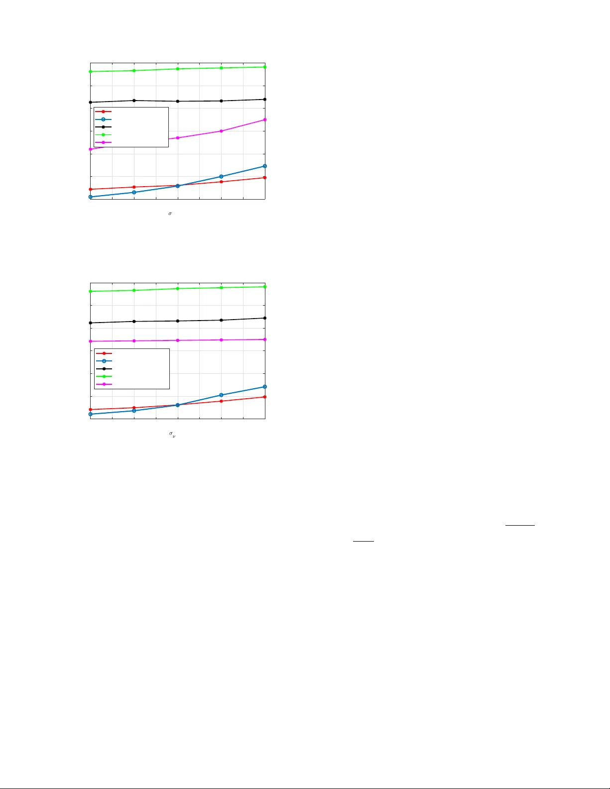
Impact of Preprocessing on Neural Network–Based RSS/AoA Positioning Omid Abbassi Aghda 1,2 , Slavisa T omic 3,4 , Oussama Ben Haj Belkacem 1,5 , Jo ˜ ao Guerreiro 1,2 , Nuno Souto 1,6 , Michal Szczachor 2,7 , and Rui Dinis 1,2 1 Instituto de T elecomunicac ¸ ˜ oes, Lisboa, Portugal 2 Univ ersidade Nov a de Lisboa, Monte da Caparica, 2829-516 Caparica, Portugal 3 UNINO V A-CTS – Center of T echnology and Systems, NO V A School of Science and T echnology , 2829-516 Caparica, Portugal 4 COPELABS, ECA TI, Lus ´ ofona Univ ersity , 1749-024 Lisbon, Portugal 5 Innov’Com Laboratory , Sup’Com, Uni versity of Carthage, T unis 1054, T unisia 6 ISCTE-Instituto Univ ersit ´ ario de Lisboa, 1649-026 Lisbon, Portugal 7 Nokia, Wroclaw , Poland Abstract —Hybrid received signal strength (RSS)/angle of ar- rival (AoA)-based positioning offers low-cost distance estimation and high-resolution angular measurements. Still, it comes at a cost of inherent nonlinearities, geometry-dependent noise, and suboptimal weighting in con ventional linear estimators that might limit accuracy . In this paper , we propose a neural network–based approach using a multilayer perceptr on (MLP) to directly map RSS/AoA measurements to 3D positions, capturing nonlinear relationships that are difficult to model with traditional methods. W e e valuate the impact of input r epresentation by comparing networks trained on raw measurements versus prepr ocessed features derived from a linearization method. Simulation results show that the learning-based approach consistently outperforms existing linear methods under RSS noise across all noise levels, and matches or surpasses state-of-the-art perf ormance under increasing AoA noise. Furthermore, prepr ocessing measurements using the linearization method provides a clear advantage over raw data, demonstrating the benefit of geometry-aware feature extraction. Index T erms —Deep learning, 3D localization, receiv ed signal strength (RSS), angle of arriv al (AoA), weighted least squares (WLS) I . I N T RO D U C T I O N Fifth-generation wireless system (5G) wireless systems are designed to support a div erse set of use cases, including en- hanced mobile broadband (eMBB), ultra-reliable low-latency communications (URLLC), and massiv e machine-type com- munications (mMTC). Beyond data transmission, these use cases increasingly rely on accurate situational awareness to en- able higher-layer applications such as Internet of Things (IoT) services, vehicle-to-e verything communication (V2X) commu- nication, unmanned aerial vehicle (U A V)s, and autonomous vehicular systems. In such applications, aw areness of the position of communicating de vices or targets, such as vehicles This work was conducted within the MiFuture project, which has received funding from the European Union’ s Horizon Europe (HE) Marie Skłodowska-Curie Actions MiFuture HORIZON-MSCA2022-DN-01, un- der Grant Agreement number 101119643 and Y AHY A/6G HORIZON-MSCA- 2022-PF-01, under Grant Agreement number 101109435. It was partially supported by FCT/MECI through national funds and when applicable co- funded EU funds under UID/50008: Instituto de T elecomunicac ¸ ˜ oes. or drones, is essential for safe and efficient operation. Conse- quently , wireless positioning has emer ged as a key enabling technology that must be addressed alongside communication performance. Looking ahead, it is widely anticipated that in sixth-generation wireless system (6G) systems, positioning and communication will be e ven more tightly integrated, with location information actively supporting communication, sensing, and control functions [1], [2]. One common approach for positioning is to use recei ved signal strength (RSS) and angle of arriv al (AoA) measure- ments collected from sensors. RSS information is attractiv e due to its low cost, while angular measurements can be obtained efficiently in multi-antenna multiple-input multiple- output (MIMO) systems. A well-studied research direction is to transform the inherently nonlinear positioning problem based on RSS and AoA into a linear form to enable closed- form solutions. For example, in [3], the authors approxi- mate the nonlinear model using a T aylor series expansion and a Cartesian-to-spherical transformation, resulting in a linearized system that can be solved via weighted least squares (WLS). Similarly , the approach in [4] applies an alternative linearization method and uses a standard least square (LS) estimator to solve the resulting system. Subsequent work in [5] extends this approach by adding constraints to the WLS cost function, reformulating it as a generalized trust region subproblem (GTRS), and solving it ef ficiently using a bisection procedure. Despite their computational efficiency , these methods remain limited in practice. RSS- and AoA- based positioning suffers from model nonlinearities, multipath propagation, and noise interference, which reduce accuracy in real-world deployments. Moreover , linearization based on T aylor approximations introduces errors, and the resulting WLS solution is generally suboptimal under realistic noise conditions [6], [7]. In addition, the weighting matrices used in WLS are typically heuristic or approximate, and non-optimal weighting can further degrade performance, especially when measurement noise is heterogeneous across anchors [7]. The use of aritifical intelegence (AI) techniques is widespread in positioning problems. In particular , deep learn- ing (DL)-based models are well suited for capturing nonlin- ear relationships and can effecti vely model the nonlinearities inherent in hybrid RSS/AoA positioning [8]. Moreov er , the positioning problem is inherently geometry-dependent, and preprocessing has a significant impact on the performance of DL-based systems [9]. Therefore, the system structure and input representation should be e xplicitly considered rather than relying solely on raw measurements. Consequently , analyzing whether to use preprocessed geometric features or raw mea- surements is essential to determine which approach enables more effecti ve learning. In this paper , we propose a neural network-based approach to address the nonlinearities inherent in hybrid RSS/AoA positioning, as studied in [3], [5]. Specifically , we design and train a multilayer perceptron (MLP) network to learn the mapping from measurements to 3D positions, capturing nonlinear relationships that are difficult to model with con ven- tional linear estimators. In addition, we ev aluate the impact of input representation by comparing networks trained on raw measurements versus preprocessed features derived from the linearization method in [3], allowing us to quantify how geometry-aware preprocessing can enhance learning perfor- mance. Although WLS approach provides a computationally ef fi- cient estimator, its performance is limited in practice due to linearization errors, noise propagation, and potentially sub- optimal weighting. By leveraging MLP, our approach can implicitly compensate for these limitations, learning a mapping that mitigates nonlinearities, weighting biases, and geometry- dependent errors, resulting in more robust positioning. T o val- idate our method, we plot the root mean square error (RMSE) versus noise v ariance for both RSS and AoA measurements. The results sho w that the MLP-based approach consistently outperforms the methods in [3]–[5] in the presence of RSS noise across all noise levels. For increasing AoA noise, the proposed method yields lower RMSE than [4], [5], while achieving RMSE performance comparable to [3]. Further- more, using the same network architecture, preprocessing the measurements via the linearization method provides a clear advantage over training with raw data, demonstrating the benefit of geometry-aware feature e xtraction. I I . P RO B L E M F O R M U L A T I O N W e consider the problem of estimating the unkno wn three- dimensional location of a target, denoted by t ∈ R 3 , which is assumed to lie within a bounded region of interest modeled as a box of size B . The positions of N anchors are known and represented by a i ∈ R 3 , i = 1 , . . . , N . Specifically , the target and anchor coordinates are gi ven by t = [ t x , t y , t z ] T and a i = [ a ix , a iy , a iz ] T , and the system geometry is illustrated in Fig. 1. For each anchor–target pair, d i , ϕ i , and α i denote the true distance, azimuth angle, and elev ation angle, respectiv ely . Fig. 1. 3d system model The distance d i , which can be estimated from the RSS at the i -th anchor is modeled as P i = P 0 − 10 γ log 10 d i d 0 + n i , (1) where P 0 is the reference power at distance d 0 (usually d 0 = 1 ), γ is the path-loss exponent, and n i ∼ N (0 , σ 2 n i ) represents the log-normal shadowing noise in the logarithmic domain. The AoA measurements are obtained using a directional antenna array and are modeled as ϕ i = arctan  t y − a iy t x − a ix  + m i , (2) α i = arccos  t z − a iz ∥ t − a i ∥  + ν i , (3) where m i ∼ N (0 , σ 2 m i ) and ν i ∼ N (0 , σ 2 ν i ) denote azimuth and elev ation measurement errors, respecti vely . T o estimate the tar get position, one can form the conditional probability density function (PDF) of the measurements giv en t . Let the observ ation vector be θ = [ p T , ϕ T , α T ] T ∈ R 3 N , where p = [ P 1 , . . . , P N ] T , ϕ = [ ϕ 1 , . . . , ϕ N ] T , and α = [ α 1 , . . . , α N ] T . Assuming independent Gaussian measurement noise, the likelihood function can be written as P ( θ | t ) = 3 Y j =1 N Y i =1 1 q 2 π σ 2 i +( j − 1) N × exp ( −  θ i +( j − 1) N − f i +( j − 1) N ( t )  2 2 σ 2 i +( j − 1) N ) , (4) where f ( t ) =  f 1 ( t ) , . . . , f 3 N ( t )  (5) =  P 0 − 10 γ log 10  d 1 d 0  , · · · , P 0 − 10 γ log 10  d N d 0  , arctan  t y − a 1 y t x − a 1 x  , · · · , arctan  t y − a N y t x − a N x  , arccos  t z − a 1 z ∥ t − a 1 ∥  , · · · , arccos  t z − a N z ∥ t − a N ∥   . (6) . Fig. 2. Illustration of the MLP-based positioning network. The model can operate on two types of inputs: preprocessed features derived from the WLS formulation (vec ( A w ) , vec ( b w ) ) or raw measurements ( p , ϕ , α ). The network consists of a linear layer , layer normalization, ReLU activation, and a final linear layer to predict the 3D target position ˆ t = [ ˆ t x , ˆ t y , ˆ t z ] T . Training is performed using the MSE loss with the Adam optimizer . Directly maximizing this likelihood is challenging due to the noncon ve xity of the resulting optimization problem. An alternativ e, suboptimal approach is the WLS solution proposed in [3], which approximates the nonlinear model as a linear system: min t ∥ W ( At − b ) ∥ , (7) with closed-form solution ˆ t = ( A T W T W A ) − 1 ( A T W T Wb ) , (8) where the matrices ha ve dimensions A ∈ R 3 N × 3 , b ∈ R 3 N × 1 , and W ∈ R 3 N × 3 N , with detailed definitions provided in the Appendix. Although WLS provides a computationally efficient estima- tor , it suffers from sev eral limitations in practical position- ing systems. Its performance relies on assumptions such as accurate linearization, Gaussian and independent noise, and correctly specified weighting, which are only approximately satisfied in practice. In particular , linearization assumes small measurement noise for all observations, but performance is much more sensitive to AoA noise than RSS noise. Small angular errors in AoA measurements can lead to large position errors due to the geometric relationship between angles and location [10]. Moreov er , linearized formulations of hybrid RSS/AoA models do not produce strictly independent Gaus- sian errors, since the linearization propagates measurement noise nonlinearly [7]. The measurement noise is also heterogeneous across an- chors, meaning that different anchors may have different variances [7]. The weighting matrix proposed in [3], while reasonable, is not guaranteed to be optimal; if it is uniform or estimated incorrectly , the WLS solution can be biased. These factors collectiv ely limit the accuracy of WLS, particularly in scenarios with high AoA noise. T o address these limitations, we propose using MLP to learn a robust mapping from the WLS input parameters to the target position. Our approach can implicitly account for nonlinearities, heterogeneous noise, and suboptimal weighting, leading to nearly constant performance across different SNR lev els, unlike con ventional WLS. I I I . D E E P L E A R N I N G B A S E D P O S I T I O N I N G T o address the limitations of WLS, including nonlinear noise propagation, heterogeneous measurement variances, and sensitivity to weighting accuracy , we consider two MLP-based positioning approaches within the same MLP architecture. The first approach lev erages the model-based preprocessing proposed in [3], while the second directly operates on raw measurements. This allows us to isolate and e valuate the impact of preprocessing on learning performance, while main- taining an identical network structure and training procedure. Figure 2 shows the MLP network architecture for the cases of raw and preprocessed inputs. A. Learning with pr epr ocessed measurements In the first approach, the MLP is trained using the linearized system parameters deri ved from the WLS formulation. Specifi- cally , the matrices A , b , and the weighting matrix W are used as input features, while the true target position t serves as the label. Each training sample is formed by preprocessing the inputs into a single feature v ector x i = [ vec ( A w ) T , vec ( b w ) T ] T ∈ R 12 N × 1 , (9) where A w = W A ∈ R 3 N × 3 and b w = Wb ∈ R 3 N × 1 . The training dataset is constructed as X = [ x 1 , . . . , x M ] ∈ R 12 N × M , Y = [ t 1 , . . . , t M ] ∈ R 3 × M , where M denotes the number of training samples and t i is the target position corresponding to x i . The MLP is trained to minimize the mean squared error (MSE) C = 1 M M X i =1 ∥ t i − ˆ t i ∥ 2 , (10) using Adam optimizer . B. Learning with r aw measurements T o ev aluate the role of model-based preprocessing, we also train an MLP using the raw measurement vector as input. In this case, the input matrix is defined as X raw = [ θ 1 , . . . , θ M ] ∈ R 3 N × M , where θ i = [ p iT , ϕ iT , α iT ] T contains the raw RSS and AoA measurements for the i -th sample. The output labels are identical to those used in the preprocessed case, i.e., Y = [ t 1 , . . . , t M ] . Apart from the input representation, only the input di- mensionality differs between the two approaches, while the network architecture, training procedure, and loss function remain identical. This setup enables a fair comparison between learning from raw measurements and learning from model- informed features deriv ed from the WLS formulation. I V . S I M U L AT I O N R E S U LT S Simulations are performed for a target constrained within a three-dimensional box of size B = 15 , with N = 4 anchors. The path-loss exponent γ is assumed to vary between 2 . 2 and 2 . 8 , while the receiv er uses a fixed value of γ = 2 . 5 . Other system parameters are P 0 = − 10 dBm and d 0 = 1 m. The WLS and LS solutions are ev aluated over 10 , 000 Monte Carlo iterations for each noise scenario. For the MLP-based estimators, the dataset contains 100 , 000 samples, of which 75% are used for training, 15% for validation, and 10% for testing. The network is trained for 300 epochs using a learning rate of 0.01. The network is trained on all SNR lev els and scenarios, while testing is performed on specific noise levels to generate the performance curves. The network architecture and training setup are summarized 1 in T able I. The MLP architecture was selected through an empirical design process. An initially overparameterized network was considered to ensure sufficient modeling capacity , after which the number of layers and neurons was progressi vely reduced to improve generalization. Batch normalization was found ineffecti ve in this setting and was therefore not adopted, while layer normalization was employed to stabilize training under varying noise conditions. The final architecture provides a fa vorable trade-off between estimation accuracy and model complexity . T o ev aluate performance, the RMSE of the estimated target positions is computed as RMSE = v u u t 1 M c M c X i =1 ∥ t i − ˆ t i ∥ 2 , (11) where M c denotes the number of Monte Carlo iterations, t i is the true target position, and ˆ t i is the corresponding estimate. For the MLP-based estimators, the input features are normal- ized to ha ve zero mean and unit v ariance, ensuring that all features hav e comparable statistical scales. This preprocessing step f acilitates stable and efficient network training across different types of measurements. The methods considered as the benchmark in this study are named as follo ws: the baseline methods from [3], [4], and [5] are referred to as WLS, LS, and SR-WLS, respectiv ely , while the proposed deep learning- based approach is referred to as ”MLP-Processed Data” and ”MLP-Raw Data”. Figure 3 shows the RMSE as a function of the RSS noise standard deviation σ n . It can be observed that the MLP- based estimator trained with preprocessed measurements using the linearization method in [3] consistently outperforms all other methods, including WLS, SR-WLS, and LS. In contrast, training the same network on raw measurements does not provide any significant improvement ov er the con ventional estimators. Figures 4 and 5 depict the RMSE versus azimuth and elev ation noise, σ m and σ ν , respectively . The results for both angular measurements are similar: MLP-preprocessed data 1 The dataset and trained networks are available at https://your- link- here. T ABLE I D N N A R C H IT E C T UR E A ND P AR A M E TE R S Layer T ype Output Size Notes / Parameters 1 Linear 128 Input: x i / θ i 2 LayerNorm 128 Normalizes features across layer 3 ReLU 128 Activ ation function 4 Linear 3 Output: ˆ t i 1 2 3 4 5 6 n (dB) 1.5 2 2.5 3 3.5 4 4.5 RMSE MLP-processed data WLS MLP-raw data LS SR-WLS Fig. 3. RMSE of the target position v ersus RSS noise standard de viation σ n i . achiev es better performance than SR-WLS and LS, while its performance is comparable to WLS. Furthermore, the advantage of using preprocessed measurements persists across all noise lev els, demonstrating that the proposed approach provides robust performance under a wide range of noise conditions. V . C O N C L U S I O N In this paper , we proposed a MLP-based approach for hy- brid RSS/AoA positioning, capturing nonlinearities that limit con ventional linear estimators. W e sho wed that preprocess- ing measurements using a linearization method significantly improv es the performance of the MLP network compared to raw data. Simulation results demonstrated that the proposed method consistently outperforms existing WLS, SR-WLS, and LS approaches under RSS and angular noise. These findings highlight that deep learning with geometry-aware preprocess- ing enables rob ust and accurate positioning across a wide range of noise conditions. R E F E R E N C E S [1] L. Italiano, B. Camajori T edeschini, M. Brambilla, H. Huang, M. Nicoli, and H. W ymeersch, “ A tutorial on 5g positioning, ” IEEE Communica- tions Surve ys & T utorials , vol. 27, no. 3, pp. 1488–1535, 2025. [2] Y . Y ang, M. Chen, Y . Blankenship, J. Lee, Z. Ghassemlooy , J. Cheng, and S. Mao, “Positioning using wireless networks: Applications, recent progress, and future challenges, ” IEEE Journal on Selected Ar eas in Communications , vol. 42, no. 9, pp. 2149–2178, 2024. [3] S. T omic, M. Beko, R. Dinis, and P . Montezuma, “ A closed-form solu- tion for rss/aoa target localization by spherical coordinates conversion, ” IEEE W ireless Communications Letters , vol. 5, no. 6, pp. 680–683, 2016. 2 3 4 5 6 7 8 9 10 m (dB) 1.5 2 2.5 3 3.5 4 4.5 MLP-processed data WLS MLP-raw data LS SR-WLS Fig. 4. RMSE of the target position versus azimuth noise standard de viation σ m i . 2 3 4 5 6 7 8 9 10 (dB) 1.5 2 2.5 3 3.5 4 4.5 MLP-processed data WLS MLP-raw data LS SR-WLS Fig. 5. RMSE of the target position versus elevation noise standard deviation σ ν i . [4] K. Y u, “3-d localization error analysis in wireless networks, ” IEEE T ransactions on Wir eless Communications , vol. 6, no. 10, pp. 3472– 3481, 2007. [5] S. T omic, M. Beko, and M. T uba, “ A linear estimator for network localization using integrated rss and aoa measurements, ” IEEE Signal Pr ocessing Letters , vol. 26, no. 3, pp. 405–409, 2019. [6] Y . Y ang, H. Y ang, and F . Meng, “ A bluetooth indoor positioning system based on deep learning with rssi and aoa, ” Sensors , vol. 25, no. 9, p. 2834, 2025. [7] S. Kang, T . Kim, and W . Chung, “Hybrid rss/aoa localization using ap- proximated weighted least square in wireless sensor networks, ” Sensors , vol. 20, no. 4, p. 1159, 2020. [8] Anonymous, “Mathematical foundations of deep learning, ” Pr eprints.org , 2025, demonstrates neural networks’ uni versal nonlinear approximation capability . [Online]. A vailable: https: //www .preprints.org/manuscript/202502.0272/v6 [9] D. Burghal, A. T . Ravi, V . Rao, A. A. Alghafis, and A. F . Molisch, “ A comprehensive survey of machine learning based localization with wireless signals, ” arXiv preprint , 2020. [10] M. H. AlSharif, M. Ba’adani, F . T oro, K. Ghamdi, S. Zahrani, M. Abdul- mohsin, and A. Al-Jarro, “In-pipe localization for pipeline intervention gadgets, ” in Abu Dhabi International P etroleum Exhibition and Confer- ence . SPE, 2023, p. D031S117R001. A P P E N D I X Assuming the noise is negligible, (1), (2), and (3) can be approximated as λ i ∥ t − a i ∥ ≈ η d 0 , i = 1 , . . . , N (12) c T i ( t − a i ) ≈ 0 , i = 1 , . . . , N (13) k T ( t − a i ) ≈ ∥ x − a ∥ cos( α i ) , i = 1 , . . . , N (14) where λ i = 10 P i / 10 γ , η = 10 P 0 / 10 γ , c i = [ − sin( ϕ i ) , cos( ϕ i ) , 0] T , k = [0 , 0 , 1] T . If each t − a i in the spherical domain is represented as t − a i = r i u i , (15) where r i > 0 is the distance from the origin and ∥ u i ∥ = 1 is the directional unit vector obtained from the AoA as u i = [cos( ϕ i ) sin( α i ) , sin( ϕ i ) sin( α i ) , cos( α i )] T , (16) then, multiplying (12), (13), and (14) by u T i u i giv es λ i u T i r i u i ≈ η d 0 ⇔ λ i u T i ( t − a i ) ≈ η d 0 , (17) k T r i u i ≈ u T i r i u i cos( α i ) ⇔ (cos( α i ) u i − k ) T ( t − a i ) ≈ 0 , (18) From (13), (17), and (18), the matrices A and b can be directly constructed as A =               . . . λ i u T i . . . c T i . . . (cos( α i ) u i − k ) T . . .               , b =               . . . λ i u T i a i + η d 0 . . . c T i a i . . . (cos( α i ) u i − k ) T a i . . .               . (19) The weighting matrix is constructed as W = I 3 ⊗ w , where I 3 denotes the 3 × 3 identity matrix and w ∈ R N × 1 contains the weighting coefficients w i = 1 − ˆ d i P N j =1 ˆ d j , with ˆ d i = d 0 10 P 0 − P i 10 γ . The symbol ⊗ denotes Kronecker product.