Pinching Antennas-Aided Integrated Sensing and Multicast Communication Systems
A pinching antennas (PAs)-aided integrated sensing and multicast communication framework is proposed. In this framework, the communication performance is measured by the multicast rate considering max-min fairness. Moreover, the sensing performance i…
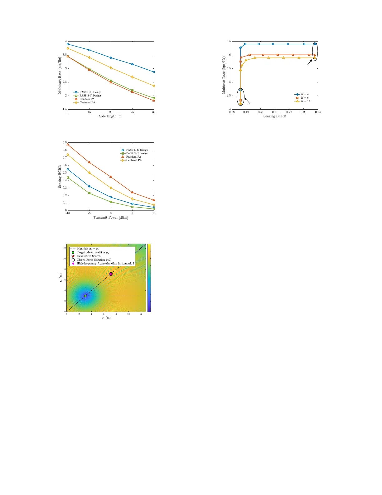
Authors: ** - Shan Shan, Yong Li – School of Information, Communication Engineering
1 Pinching Antennas-Aided Inte grated Sensing and Multicast Communication Systems Shan Shan, Chongjun Ouyang, Xiaohang Y ang, Y ong Li, Zhiqin W ang, and Y uanwei Liu Abstract —A pinching antennas (P As)-aided integrated sensing and multicast communication framework is pr oposed. In this framework, the communication performance is measured by the multicast rate considering max-min fairness. Mor eover , the sensing performance is quantified by the Bayesian Cram ´ er - Rao bound (BCRB), where a Gauss-Hermite quadrature-based approach is pr oposed to compute the Bayesian Fisher inf ormation matrix. Based on these metrics, P A placement is optimized under three criteria: communications-centric (C-C), sensing-centric (S- C), and Pareto-optimal designs. These designs are in vestigated in two scenarios: the single-P A case and the multi-P A case. 1) For the single-P A case, a closed-form solution is derived f or the location of the C-C transmit P A, while the S-C design yields optimal transmit and receive P A placements that are symmetric about the target location. Leveraging this geometric insight, the Par eto-optimal design is solved by enfor cing this P A placement symmetry , thereby reducing the joint transmit and receiv e P A placement to the transmit P A optimization. 2) For the general multi-P A case, the P A placements constitute a highly non-conv ex optimization problem. T o solve this, an element-wise alternating optimization-based method is proposed to sequentially optimize all P A placements for the S-C design, and is further incorpo- rated into an augmented Lagrangian (AL) framework and a rate-profile formulation to solve the C-C and Pareto-optimal design problems, respectively . Numerical results show that: i) P ASS substantially outperforms fixed-antenna baselines in both multicast rate and sensing accuracy; ii) the multicasting gain becomes more pronounced as the user density incr eases; and iii) the sensing accuracy improves with the number of deploy ed P As. Index T erms —Bayesian Cram ´ er -Rao bound (BCRB), inte- grated sensing and communications (ISA C), pinching-antenna system (P ASS). I . I N T RO D U C T I O N Integrated sensing and communications (ISA C) combines dual communication and sensing functionalities over shared wireless resources to improv e spectrum utilization and system efficienc y [1], [2]. Multiple-input multiple-output (MIMO) technology has been widely regarded as an efficient approach to ISA C, as it lev erages spatial diversity and beamforming to simultaneously enhance spectral efficienc y and sensing accuracy [3], [4]. Howe ver , con ventional MIMO architectures remain constrained by their geometrically fix ed antenna con- figurations, which limit their adaptability to dynamic prop- agation en vironments. T o ov ercome this limitation, flexible- antenna systems ha ve been proposed as an emerging antenna paradigm that enhance the spatial adaptability of wireless Shan Shan and Y ong Li are with the School of Information and Commu- nication Engineering, Beijing Uni versity of Posts and T elecommunications, Beijing 100876, China (e-mail: { shan.shan, liyong } @bupt.edu.cn). Chongjun Ouyang is with the School of Electronic Engineering and Computer Sci- ence, Queen Mary University of London, London E1 4NS, U.K. (e-mail: c.ouyang@qmul.ac.uk). Xiaohang Y ang and Zhiqin W ang are with China Academy of Information and Communications T echnology , Beijing 100876, China (e-mail: { yangxiaohang, wangzhiqin } @caict.ac.cn). Y uanwei Liu is with the Department of Electrical and Electronic Engineering, The University of Hong K ong, Hong Kong (e-mail: yuanwei@hku.hk). channels. Representativ e implementations include mov able- antenna and fluid-antenna architectures [5], [6]. Mov able an- tennas change their physical posit ions to modify link geometry , while fluid antennas reshape their electromagnetic aperture through conducti ve-fluid redistribution. By locally adapting the propagation path, they can mitigate small-scale fading and im- prov e both communication reliability and sensing accuracy in ISA C systems. In addition, reconfigurable intelligent surfaces (RISs) [7] have also been introduced to mitigate propagation blockages. By le veraging controllable phase shifts of numer - ous passive reflecting elements, RIS technology establishes reliable virtual links between the base station (BS) and sensing targets. Howe ver , the effecti veness of mov able-antenna and fluid-antenna is generally constrained by limited mov ement ranges, which restricts their capability in addressing large- scale path-loss or line-of-sight (LoS) blockage. Meanwhile, RIS encounters a se vere double path-loss effect, especially at higher operating frequencies, which substantially degrades its reflection efficienc y . Recently , the Pinc hing-Antenna SyStem (P ASS) has been ex- perimentally demonstrated as a practical realization of flexible- antennas that addresses the aforementioned limitations [8], [9]. P ASS employs a dielectric wav eguide as the transmission medium with low in-wav eguide propagation loss, and its aper- ture length spans from a few meters to tens of meters. Along the wa veguide, small dielectric elements, termed pinching antennas (P As), can be dynamically attached or detached, from which radio wav es are transmitted or receiv ed. A key advantage of P ASS for ISA C lies in its scalable wa ve guide structure, which can be extended to be arbitrarily long. From a communication perspectiv e, this establishes “near-wir ed” links with strong LoS conditions to indi vidual users. This characteristic effecti vely mitigates large scale path-loss and av oid LoS blockage [10]. Simultaneously , the long wav eguide synthesizes a large effecti ve aperture for sensing, which in- duces dominant near-field effects that facilitate precise polar domain localization [11]. A. Related W orks The above adv antages have motiv ated sev eral early in- vestigations into P ASS-enabled communications and sensing. In particular , the authors in [12] provided an information- theoretic characterization of the achiev able rate region for P ASS-aided ISAC systems, which rev ealed a fundamental tradeoff between communication and sensing rates. Extending this analysis, the studies in [13]–[15] in vestigated the integra- tion of P ASS into ISA C systems, where the receiv ed signal- to-noise ratio (SNR) at the sensing targets was adopted as the performance metric. T o obtain a more rigorous measure, sub- sequent studies adopted the Cram ´ er-Rao bound (CRB), which provides the theoretical lower bound on the estimation error 2 variance of any unbiased estimator [16], [17]. Specifically , the CRB achieved by P ASS is first deriv ed in [18] and then com- pared to that of con ventional antennas, while [19] in vestigated its minimization via a particle swarm optimization (PSO)- based algorithm. In parallel, works such as [20]–[22] analyzed round-trip sensing configurations using uniform linear arrays (ULAs) for echo reception. From an architectural perspective, the segmented wa veguide system (SW AN) in [23] enhances the degrees of freedom (DoF) av ailable for optimization and characterizes the Pareto fronts for sensing and communication performance. Building on these theoretical foundations, recent works hav e extended the framework to div erse scenarios. T o adapt to high-mobility en vironments, the work in [24] proposed a P ASS-enabled ISAC framew ork for unmanned aerial vehicles (U A Vs) utilizing deep reinforcement learning, while the authors in [25] addressed security concerns by jointly optimizing P A locations and artificial noise. Furthermore, to improv e transmission ef ficiency , the work in [26] introduced an index modulation (IM)-based framew ork, which employs variational inference for joint user localization and symbol detection. Collecti vely , these studies establish the theoretical foundation for P ASS-aided ISA C systems and demonstrate the validity and ef fecti veness of P ASS-enabled architectures. B. Motivations and Contributions Despite the significant progress achiev ed by these works, two critical issues remain unresolved in P ASS-aided ISA C research. First, most existing sensing designs adopt the CRB as the metric under the idealized assumption that the parameters to be sensed are deterministic and kno wn. In practice, howe ver , the target parameters are typically unknown and random. Fortunately , their prior probability density functions (PDFs) can be obtained based on target properties and historical data. In such cases, the Bayesian CRB (BCRB) provides a more appropriate lower bound on the sensing mean-squared error (MSE) by explicitly exploiting the prior distribution informa- tion [27]–[29]. Second, regarding the communication func- tionality , existing P ASS-enabled ISA C studies largely focus on single-user or unicast transmission. Ho we ver , multicasting naturally aligns with the hardware characteristics of P ASS. Since the wave guide is connected to a single RF chain, the av ailable spatial DoF for mitigating inter-user interference are inherently limited, which makes this architecture more fa vorable for multicast transmission. By deliv ering a common message, multicasting a voids user-specific streams and thus further alleviates the DoF limitation of P ASS-enabled mul- tiuser transmission. Ne vertheless, this important P ASS-enabled multicast ISA C scenario remains largely unexplored. T o fill these research gaps and to obtain a deeper under- standing of the communications-sensing tradeof f in P ASS- enabled ISA C systems, we propose a P ASS-aided integrated sensing and multicast communication framework. The major contributions of this paper are summarized as follows: • W e propose a P ASS-aided ISAC framew ork where the P A placement is optimized to perform simultaneous in- formation multicasting and target sensing. W ithin this framew ork, the multicast communication performance is quantified by the max-min fairness (MMF) rate, while the BCRB is adopted to characterize the relationship between the P A placement and sensing accuracy . Since the BCRB e valuation inv olves intractable integrals, the Gauss-Hermite quadrature (GHQ) rule is employed to facilitate the computation of the Fisher information ma- trix (FIM). Based on these metrics, the P A placement optimization is then in vestigated under three design cri- teria, namely: 1) communications-centric (C-C) design, which maximizes the multicast rate, 2) sensing-centric (S-C) design, which minimizes the BCRB, and 3) P areto- optimal design, which characterizes the communications- sensing tradeoff. • W e start from a single-P A setup to rev eal ke y design insights and to characterize the Pareto boundary . i) For the C-C design, we deri ve a closed-form solution in which the optimal transmit P A lies in a finite candidate set. ii) For the S-C design, we deri ve that under one-dimensional target location uncertainty , the optimal transmit and re- ceiv e P A placements admit a symmetric layout. iii) For the Pareto-optimal design, we adopt a rate-profile-based formulation to characterize the tradeof f boundary . By exploiting the fact that the multicast rate is independent of the receiv e P A, the recei ve P A placement follo ws a closed-form sensing-driv en symmetry rule, and the remaining transmit P A placement reduces to an ef ficient univ ariate optimization that can be solved via a simple one-dimensional search. • W e further extend our study to the multi-P A setting, where a more rigorous design is considered by explicitly accounting for performance constraints beyond the objec- tiv e. i) For the S-C design, we propose an element-wise alternating optimization (A O) method to sequentially optimize all P A placements so as to minimize the BCRB under a minimum multicast rate constraint. ii) For the C-C design, we dev elop a penalty-based adaptation to maximize the multicast rate subject to a maximum BCRB constraint. iii) For the Pareto-optimal design, we propose a rate-profile-based scalarization approach to characterize the tradeoff boundary and solve the resulting problem using the sequential element-wise A O algorithm. • Finally , we provide numerical results to validate the effecti veness of the proposed algorithms. Our findings rev eal that: i) P ASS achiev es substantial performance gains over con ventional fixed-location antenna systems in both multicast communication and sensing performance. ii) For multicasting, the performance advantage of P ASS becomes more pronounced in scenarios with high user density . iii) For sensing, the deplo yment of additional P As yields increasingly precise tar get localization. The reminder of this paper is organized as follows. Sec- tion II presents the P ASS-ISA C system model and perfor- mance metrics. Section III and IV optimize the P A placement in a simplified single-P A scenario and a more general multi-P A scenario, respectively . Section V provides numerical results. Finally , Section VI concludes the paper . Notations: Scalars, vectors, and matrices are represented by regular , bold lo wercase, and bold uppercase letters, respec- tiv ely . The sets of comple x and real numbers are denoted by 3 Tx - PA S S Rx - PASS m ulti cast us e r se nsin g target BS Fig. 1. Illustration of P A-aided integrated sensing and multicast transmission. C and R . The operators ( · ) − 1 , ( · ) ∗ , ( · ) T , ( · ) H , and tr ( · ) corre- spond to the in verse, conjugate, transpose, conjugate transpose, and trace, respecti vely . For a vector x , [ x ] i represents its i th element, while Diag ( x ) constructs a diagonal matrix using the elements of x . The Kronecker delta is denoted by δ ( x, y ) , which equals 1 if x = y and 0 otherwise. The operator [ x ] + ≜ max { x, 0 } represents the non-negativ e projection of x . C N ( a, b 2 ) signifies a circularly symmetric complex Gaussian distribution with mean a and variance b 2 . The statistical expectation is giv en by E {·} . Furthermore, | · | and ∥ · ∥ denote the absolute value and Euclidean norm, respecti vely . Finally , ℜ{·} extracts the real part of a complex number , and O ( · ) denotes the big-O notation. I I . S Y S T E M M O D E L W e consider a P ASS-aided ISA C system that simultaneously performs information multicasting and sensing. The dual- functional BS is equipped with a transmit wa ve guide ( Tx- P ASS ) employing N t Tx-P As and a receive wa veguide ( Rx- P ASS ) employing N r Rx-P As. Both wave guides and their as- sociated P As are deployed at a fixed height h above the ground, within a rectangular co verage area of size D x × D y . For practical deployment, the Tx-P ASS and Rx-P ASS are aligned parallel to the x -axis. The feed points of the Tx-P ASS and Rx- P ASS are located at ψ t , 0 ≜ [0 , y t , h ] T and ψ r , 0 ≜ [0 , y r , h ] T , respectiv ely , where y t and y r denote their positions along the y -axis. Define N t ≜ { 1 , . . . , N t } and N r ≜ { 1 , . . . , N r } as the index sets of Tx-P As and Rx-P As, respecti vely . The location of the n th Tx-P As and Rx-P As are denoted by ψ t ,n ≜ [ x t ,n , y t , h ] T , ∀ n ∈ N t and ψ r ,n ≜ [ x r ,n , y r , h ] T , ∀ n ∈ N r , respectiv ely . Let x t ≜ [ x t , 1 , x t , 2 , . . . , x t ,N t ] T collect the x - coordinate of all Tx-P As. These coordinates satisfy the spatial constraint 0 ≤ x t , 1 < · · · < x t ,N t ≤ D x and a minimum inter- P A spacing constraint | x t ,n − x t ,n − 1 | ≥ ∆ min = λ 2 , ∀ n ∈ N t , n ≥ 2 , where λ is the free-space wavelength [30]. The x -coordinates of the Rx-P As follow the same constraints. The considered ISA C system simultaneously serves K single-antenna user and senses a single target, as illustrated in Fig. 1. Let K ≜ { 1 , 2 , . . . , K } denote the index sets of the users. The position of the k th user is denoted by ξ k ≜ [ v x k , v y k , 0] T , whereas the target is assumed to be located at ζ ≜ [ u x , u y , 0] T . The BS simultaneously transmits common information signals to all users and utilizes the reflected echo signals for sensing. Moreov er , we focus on the fundamental sensing process and neglect the potential interference of down- link communication signals on the recei ved echoes, which assumes that such coupling effects can be effecti vely mitigated through standard self-interference cancellation and synchro- nization techniques [2]. Let s ∈ C denote the ISA C transmit signal emitted by the BS. The BS is subject to a maximum transmit po wer budget of P t , where P t = 1 . T o achie ve the multicast capacity limit under this power constraint, the transmitted signal is s = √ P t s o , where s o ∼ C N (0 , 1) denotes the normalized information symbol. A. Multicast Communication P erformance Metric W e first consider the multicast communication channel. Let h ( ξ k , x t ) ∈ C N t × 1 denote the channel vector from the BS to user k ∈ K . The signal received by the k th user is y k = h T ( ξ k , x t ) ϕ t ( x t ) s + z k , ∀ k ∈ K , (1) where z k ∼ C N (0 , σ 2 k ) represents the additiv e noise at the k th user with noise v ariable σ 2 k . The n th element of h ( ξ k , x t ) represents the free-space channel coef ficient between the n th Tx-P A and the k th user , which can be expressed as follo ws: [ h ( ξ k , x t )] n ≜ √ η e − j k 0 ∥ ξ k − ψ t ,n ∥ ∥ ξ k − ψ t ,n ∥ . (2) Here, k 0 = 2 π λ is the wa venumber , and η ≜ c 2 16 π 2 f 2 c with c and f c denoting the speed of light and the carrier frequency , respectiv ely . Moreov er , the n th element of ϕ t ( x t ) represents the normalized in-wa ve guide propagation coef ficient between the Tx-P As and the feed point of the Tx-P ASS, which can be written as follows: [ ϕ t ( x t )] n = r 1 N t exp ( − j k g ∥ ψ t ,n − ψ t , 0 ∥ ) , (3) where k g = 2 π λ g is the in-wave guide wavenumber with λ g denoting the in-wa veguide wa velength. Based on the recei ved signal model in (1), the received SNR at the k th user can be written as follows: γ k ( x t ) ≜ E | h T k ( ξ k , x t ) ϕ t ( x t ) s | 2 | z k | 2 = P t | h T k ( ξ k , x t ) ϕ t ( x t ) | 2 σ 2 k . (4) Accordingly , the achiev able MMF rate with a given transmit P A location vector x t is determined by the minimum SNR among all multicast users, which can be gi ven by [31] R c ( x t ) = min k ∈K n log 2 1 + γ k ( x t ) o . (5) B. Sensing P erformance Metric Next, we consider the P ASS-based sensing model, in which the multicast signals transmitted by the Tx-P ASS are reflected by the target and subsequently collected by the Rx-P ASS for sensing the location of the target. Specifically , the received echo signal is modeled as follows: y s = β s h ( ζ , x r ) h T ( ζ , x t ) ϕ t ( x t ) s + z s , (6) where z s ∼ C N ( 0 , σ 2 s I N r ) represents the additi ve CSCG noise vector , and β s denotes the complex target scattering coefficient associated with the radar cross-section (RCS). Here, we treat β s as a deterministic constant within one coherent processing interval and absorb it into a normalized gain factor , e.g., β s = 1 without loss of generality [32], so that the sensing performance is dominated by the geometric dependence on ζ . Moreov er , the vectors h ( ζ , x t ) ∈ C N t × 1 4 and h ( ζ , x r ) ∈ C N r × 1 denote the free-space channel vectors between the target and the Tx/Rx-P ASS, respectiv ely , and are defined in the same form as those in (2). Denote X ≜ [ x t x r ] T and G ( ζ , X ) ≜ h ( ζ , x r ) h T ( ζ , x t ) . Then, the corresponding baseband observation at the BS can be expressed as follows: ˆ s ≜ ϕ T r ( x r ) y s = β s ϕ T r ( x r ) G ( ζ , X ) ϕ t ( x t ) s + ˜ z s . (7) Here, ϕ r ( x r ) ∈ C N r × 1 denotes the normalized in-wav eguide propagation vector from the Rx-P As to the feed point of the Rx-P ASS, which follows the same modeling principle as ϕ t ( x t ) in (3). The ef fectiv e noise after combining is giv en by ˜ z s = ϕ T r ( x r ) z s ∼ C N (0 , σ 2 s ) . Conditioned on the unknown target parameters ζ , ˆ s is a complex Gaussian distribution as follows: ˆ s ∼ C N µ ( ζ , X ) , σ 2 s , (8) where µ ( ζ , X ) = β s ϕ T r ( x r ) G ( ζ , X ) ϕ t ( x t ) s. (9) Upon recei ving ˆ s , the BS estimates the target locations, yielding an estimate ˆ ζ . The sensing accuracy is quantified via the mean-square error (MSE), which is defined as follo ws: MSE ζ ≜ E n ∥ ˆ ζ − ζ ∥ 2 2 o . (10) Since the sensing MSE is difficult to express analytically , we adopt the BCRB as the sensing performance metric, which provides a theoretical lo wer bound on the MSE [33], [34]. Specifically , the BCRB satisfies MSE ζ ≥ BCRB ( X ) = tr F − 1 ( ζ , X ) , (11) where F ( ζ , X ) ∈ R 2 × 2 denotes the Bayesian Fisher infor- mation matrix (BFIM) associated with the target location parameter vector ζ . It consists of two additi ve components, namely the observation Fisher information and the prior Fisher information, which satisfies [35] F ( ζ , X ) = e F ( ζ , X ) + F p ( ζ ) . (12) Here, e F ( ζ , X ) represents the Fisher information contributed by the observation model, and F p ( ζ ) captures the prior information determined by the statistical distribution of ζ . 1) PFIM Derivation: The prior Fisher information matrix (PFIM) quantifies the prior kno wledge re garding ζ , which is defined as follows [36]: F p ( ζ ) ≜ − E ζ ∇ 2 ζ ln p ( ζ ) . (13) For analytical tractability , we model the target coordinates as independent Gaussian random variables 1 , i.e., u α ∼ N ( µ α , σ 2 α ) for α ∈ { x, y } . Here, the mean µ α represents the predicted target location deriv ed from historical observ ations, while the variance σ 2 α characterizes the associated uncertainty . Substituting the independent Gaussian PDFs into (13), the log- prior becomes a quadratic function, and the PFIM is deriv ed as the inv erse of the prior cov ariance matrix as follo ws: F p ( ζ ) = Diag σ − 2 x , σ − 2 y . (14) Note that the off-diagonal elements v anish due to the statistical independence between the x and y -coordinates. 2) OFIM Derivation: Similar to the PFIM defined in (13), the observation Fisher information matrix (OFIM) is defined 1 While this work adopts a Gaussian prior for tractability , the framework can be extended to more general distributions, such as Gaussian mixtures, which remains a promising direction for future research. as follows [36]: e F ( ζ , X ) ≜ E ζ ∇ ζ ln p ( ˆ s | ζ , X ) ∇ ζ ln p ( ˆ s | ζ , X ) T . (15) For our CSCG model in (8), the OFIM admits the closed form as follows: e F ( ζ , X ) = 2 σ 2 s E ζ h ℜ n ∇ ζ µ H ∇ ζ µ oi ≜ 2 σ 2 E ζ h ℜ n J H ( ζ , X ) J ( ζ , X ) oi , (16) where J ( ζ , X ) = ∂ u x µ ∂ u y µ ≜ f x ( ζ , X ) f y ( ζ , X ) . (17) By introducing the unified deri vati ve kernel K p,n α ( ζ , X ) ≜ η 1 2 [ ϕ p ( x p )] n e − j k 0 R p,n χ p,n α 1 + j k 0 R p,n R 3 p,n , (18) where χ p,n x = u x − x p,n , χ p,n y = u y with α ∈ { x, y } , p ∈ { t , r } , the functions f x and f y in (17) can then be expressed as follows: f α ( ζ , X ) = − g t ( ζ , x t ) N t X n =1 K t ,n α − g r ( ζ , x r ) N r X n =1 K r ,n α , (19) where g t ( ζ , x t ) = h T ( ζ , x t ) ϕ t ( x t ) and g r ( ζ , x r ) = h T ( ζ , x r ) ϕ r ( x r ) represent the effecti ve channels for the Tx- P ASS and Rx-P ASS, respectively . Consequently , the OFIM in (16) is gi ven by e F ( ζ , X ) = 2 P t σ 2 s " e F xx ( ζ , X ) e F xy ( ζ , X ) e F y x ( ζ , X ) e F y y ( ζ , X ) # , (20) where e F αβ ( ζ , X ) ≜ E ζ [ ℜ { f ∗ α ( ζ , X ) f β ( ζ , X ) } ] (21) for α, β ∈ { x, y } . For the diagonal elements when α = β , taking the case of α = β = x as an example and substituting the factorized Gaussian prior density p ( ζ ) into (21) yields e F xx ( ζ , X ) = ℜ Z Z R 2 f x ( ζ , X ) 2 p ( u x ) p ( u y ) d u x d u y . (22) By applying the standard variable substitution u x = µ x + σ x ν and u y = µ y + σ y η , and noting that p ( u x )d u x = e − ν 2 √ π d ν and p ( u y )d u y = e − η 2 √ π d η , we rewrite the integral in (22) into the canonical Gauss-Hermite form as follo ws: e F xx ( ζ , X ) = ℜ 1 π Z Z R 2 f x ( µ x + σ x ν, µ y + σ y η ) 2 e − ν 2 e − η 2 d ν d η o . (23) Howe ver , the expectations in (23) do not yield closed-form expressions. T o address this, we adopt the Gauss-Hermite quadrature (GHQ) rule R + ∞ −∞ ψ ( x ) e − x 2 d x ≈ P T i =1 ω i ψ ( ξ i ) to approximate the integrals, where { ω i } and { ξ i } denote the weight and abscissa factors of Gauss-Hermite integration, and T is a complexity-vs-accurac y tradeof f parameter . Accord- ingly , we approximate the FIM entries as follo ws: e F xx ( ζ , X ) ≈ T X i =1 T X j =1 ω i ω j ℜ n 1 π f x ( µ x + √ 2 σ x ξ i , µ y + √ 2 σ y ξ j ) 2 o . (24) The term e F y y ( ζ , X ) follows an identical deri vation by replac- ing the partial deri v ativ e f x ( · ) with f y ( · ) . For the off-diagonal entries when α = β , the expectation must be e valuated o ver the coupled product of the deri v ativ es. 5 Accordingly , the GHQ approximation is applied to the joint term as follows: e F xy ( ζ , X ) ≈ T X i =1 T X j =1 ω i ω j ℜ n 1 π f ∗ x ( µ x + √ 2 σ x ξ i , µ y + √ 2 σ y ξ j ) · f y ( µ x + √ 2 σ x ξ i , µ y + √ 2 σ y ξ j ) o . (25) Finally , the v alue of e F y x ( ζ , X ) is obtained via the Hermitian symmetry of the FIM, i.e., e F y x = e F xy . Since both e F ( ζ , X ) and F p ( ζ ) are of order 2 × 2 , the matrix inv ersion can be calculated in a closed-form, which yields BCRB ( X ) = tr F − 1 ( ζ , X ) = e F xx + e F y y + σ − 2 x + σ − 2 y ( e F xx + σ − 2 x )( e F y y + σ − 2 y ) − | e F xy | 2 . (26) It is clear that both the multicast rate in (5) and the BCRB in (26) depend critically on the P A placement. In general, the P A configuration that is optimal for sensing is not optimal for multicasting, which gi ves rise to an inherent sensing- communications tradeoff. T o characterize and na vigate this tradeoff, we consider three complementary design criteria: 1) S-C design, which minimizes the BCRB subject to a multicast- rate requirement; 2) C-C design, which maximizes the MMF multicast rate subject to a sensing-accuracy requirement; and 3) Pareto-optimal design, which characterizes the achiev able sensing-communications tradeof f by tracing the Pareto bound- ary via a rate-profile formulation. I I I . S I N G L E - P A C A S E In this section, we first in vestig ate a single-P A setting to deriv e the optimal solution to P A placement for the S-C, C-C, and Pareto-optimal designs. A. Communications-Centric Design Since the downlink multicast rate depends only on the Tx- P A placement, the C-C design simplifies to max x t R c ( x t ) , s.t. x t ∈ [0 , D x ] . (27) For the k th user located at ( ˆ x c ,k , ˆ y c ,k ) , the receiv ed SNR under a single Tx-P A located at x t is γ k ( x t ) = σ − 2 k P t [( x t − ˆ x c ,k ) 2 + ( y t − ˆ y c ,k ) 2 + h 2 ] − 1 . (28) Therefore, maximizing the multicast rate is equiv alent to minimizing the maximum distance between the Tx-P A and all multicast users, which can be expressed as follo ws: min x t max k ∈K ( x t − ˆ x c ,k ) 2 + ∆ 2 k , (29) where ∆ 2 k ≜ ( y t − ˆ y c ,k ) 2 + h 2 . Define d k ( x ) ≜ ( x − ˆ x c ,k ) 2 + ∆ 2 k and d ( x ) ≜ max k ∈K d k ( x ) . Each d k ( x ) is a con ve x quadratic function of x , and hence d ( x ) is also con ve x on [0 , D x ] . Since d k ( x ) attains its unique minimum at x = ˆ x c ,k , each d k ( x ) is strictly unimodal. As d ( x ) represents the upper env elope of these con ve x curv es, the global minimizer of d ( x ) must occur at a point where either i) a single curve d k ( x ) reaches its minimum, or ii) two curves intersect and yield equal values. Consequently , a closed-form structure of the optimal trans- mit P A placement can be established by identifying a finite candidate set that guarantees optimality . Specifically , the op- timal Tx-P A position can be determined from the following finite candidate set: i) the set of multicast users’ x -coordinates, X 1 ≜ { ˆ x c , 1 , . . . , ˆ x c ,K } ; and ii) the set of pairwise equal- distance points, X 2 ≜ { ξ i,j | d i ( ξ i,j ) = d j ( ξ i,j ) , i < j } , where each intersection point ξ i,j is giv en by ξ i,j = ∆ 2 j − ∆ 2 i 2( ˆ x c ,j − ˆ x c ,i ) + ˆ x c ,i + ˆ x c ,j 2 . (30) Including the boundary points, the complete candidate set is G c = { 0 , D x } ∪ X 1 ∪ X 2 . Finally , the globally optimal Tx-P A placement for the C-C design is obtained by ev aluating the multicast objectiv e at all candidate points in G c as follows: x ⋆ t = arg min x ∈G c max k ∈K ( x − ˆ x c ,k ) 2 + ∆ 2 k . (31) B. Sensing-Centric Design Obtaining closed-form expressions for the optimal Tx- and Rx-P A placements that minimize the BCRB in (26) is in general intractable, because the sensing performance depends on the joint Tx- and Rx-P A placement. In particular , the of f- diagonal terms of the BFIM couple the two variables, so that the optimal Tx-P A location depends on the Rx-P A location and vice versa. Consequently , the first-order optimality conditions lead to coupled nonlinear equations in ( x t , x r ) , for which a closed-form solution is generally unav ailable. T o expose the key geometric structure of the S-C design, we therefore adopt a simplified symmetric setup in which the target lies on the perpendicular bisector of the two w ave guides. Specifically , we treat its y -coordinate as known and fixed at u y = y t + y r 2 . Under the single-P A configuration, the Euclidean distances between the target and the Tx- or Rx-P As are expressed as follows: R t = p ( u x − x t ) 2 + ∆ 2 s , R r = p ( u x − x r ) 2 + ∆ 2 s , (32) where ∆ s = q h 2 + y r − y t 2 2 . Consequently , we focus the estimation solely on the x -coordinate u x . Based on this as- sumption, the mean of the received echo signal in (9) simplifies to the following: µ ( u x , x t , x r ) = C e − j k 0 ( R t + R r ) R t R r , (33) where C ≜ β s √ η P t e − j k g ( x t + x r ) aggregates the system scaling factors and the phase shift introduced by in-wav eguide propa- gation. Since the unknown parameter reduces to the scalar u x , the conditional observation Fisher information for estimating u x is a scalar quantity , denoted by F xx ( u x , x t , x r ) . T aking the prior expectation over u x , the corresponding scalar OFIM entry in (20) can be simplified as follo ws: e F ( u x , X ) = e F xx ( u x , x t , x r ) ≜ E u x F xx ( u x , x t , x r ) . (34) Accordingly , the one-dimensional BFIM becomes F ( x t , x r ) = e F xx ( u x , x t , x r ) + σ − 2 x , and the BCRB in (26) simplifies to BCRB ( u x , x t , x r ) = e F xx ( u x , x t , x r ) + σ − 2 x − 1 . (35) For a fixed prior term σ − 2 x , improving the sensing accuracy is thus equiv alent to increasing e F xx ( u x , x t , x r ) . Consequently , we formulate the S-C design problem as follo ws: max { x t ,x r } e F xx ( u x , x t , x r ) , s.t. x t ∈ [0 , D x ] , x r ∈ [0 , D x ] . (36) T o make the dependence of the sensing information on the P A placement explicit, we next rewrite the conditional Fisher information in terms of the LoS distances and angles. Specif- ically , define the direction cosine of the Tx/Rx links along 6 the x -axis as cos θ p ≜ ( u x − x p ) /R p for p ∈ { t , r } . Then, the conditional Fisher information for estimating u x can be expressed as follows: F xx ( θ t , θ r ) = 2 | µ | 2 σ 2 s h k 2 0 + R − 2 t cos θ 2 t + k 2 0 + R − 2 r cos θ 2 r + 2 k 2 0 + ( R t R r ) − 1 cos θ t cos θ r Φ i , (37) where Φ ≜ cos k 0 ( R t − R r ) , and | µ | 2 denotes the path-loss dependent signal power . Directly solving (36) is still challenging, because it inv olves a prior expectation and the conditional term F xx ( u x , x t , x r ) is highly non-conv ex with respect to (w .r .t.) the transmit and receiv e P A placements. T o obtain a tractable design with clear physical insight, we proceed in two steps. First, for a fixed target realization u x , we study the conditional Fisher informa- tion F xx ( u x , x t , x r ) and show that it is maximized when the Tx-P A and Rx-P A are placed symmetrically around u x along the x -axis (see Proposition 1). This restricts the transcei ver layout to a symmetric manifold that can be parameterized by a center c and a nonnegati ve displacement d . Second, under a symmetric prior for u x , we show that the Bayes-optimal center is c = µ x (see Proposition 2), which leads to a closed-form displacement summarized in Remark 1. Proposition 1. F or any given tar get x -coor dinate u x , under the symmetric setup u y = ( y t + y r ) / 2 , the conditional observation Fisher information F xx ( u x , x t , x r ) is maximized when the Tx-P A and Rx-P A ar e placed symmetrically around the tar get along the x -axis, i.e., | u x − x t | = | u x − x r | . Pr oof: Please refer to Appendix A. Motiv ated by Proposition 1, we parameterize this symmetric design class by a symmetry center c and a nonnegati ve x - axis displacement d ≥ 0 (i.e., d is the absolute x -coordinate difference from the center), namely M ( c ) ≜ n ( x t , x r ) x t = c ± d, x r = c ± d, d ≥ 0 o . (38) Restricting ( x t , x r ) to M ( c ) reduces the two-dimensional placement to a one-dimensional search ov er d for any fix ed c . W e select the same-side branch x t = x r = c − d . In contrast, for the opposite-side equal-offset placement x t = c − d and x r = c + d , the geometric placement implies R t = R r and cos θ r = − cos θ t , Substituting these relations into (37) shows that the bracketed term cancels, and hence F xx = 0 . Moreov er , under a symmetric prior on µ x , the Bayes-aligned center is attained at the prior mean c = µ x , as established in Proposition 2. Proposition 2. Assume that the prior of u x is symmetric about µ x . Consider the OFIM r estricted to the equal-offset manifold M ( c ) , i.e., e F xx ( c, d ) ≜ E u x F xx ( u x , c, d ) . The OFIM is stationary w .r .t. the center at the prior mean, i.e., ∂ c e F xx ( c, d ) c = µ x = 0 , which motivates choosing c = µ x as the canonical Bayes-aligned center under a symmetric prior . After that, the derivative of the OFIM w .r .t. d admits d d d E u x F xx ( u x , d ) = ∂ d F xx ( µ x , d ) + O ( σ 2 x ) , (39) Pr oof: Please refer to Appendix B. By setting the first deriv ative of (39) to zero, we obtain the optimal x -axis displacement d ⋆ , summarized in the following remark. Remark 1. The closed-form expr ession of the optimal dis- placement is ( d ⋆ ) 2 = − ( k 2 0 ∆ 2 s + 3) + p 9 k 4 0 ∆ 4 s + 14 k 2 0 ∆ 2 s + 9 4 k 2 0 . (40) In the typical high-fr equency re gime of P ASS wher e k 0 ∆ s ≫ 1 , it further admits the appr oximation d ⋆ ≈ ∆ s / √ 2 . Pr oof: Please refer to Appendix C. By additionally incorporating the in-wav eguide propagation loss, the resulting closed-form P A placement becomes x ⋆ t = x ⋆ r = µ x − d ⋆ . (41) This result highlights a non-intuiti ve but important design insight: an intuition is to place the P A as close to the tar get as possible, i.e., x t = x r = µ x (equiv alently , d → 0 ). Ho we ver , (40) sho ws that this intuition is generally incorrect: the optimal displacement d ⋆ is a function of the effecti ve height ∆ s , which is consistent with the observ ation in [18]. C. P areto-Optimal Design Building on the preceding C-C and S-C designs, we now characterize the fundamental communications-sensing tradeoff via the rate-profile scalarization framew ork. Specifically , we define the sensing rate as the in verse of the BCRB, i.e., R s ( x t , x r ) ≜ BCRB ( x t , x r ) − 1 . For a gi ven α , a Pareto- optimal point is obtained by solving max x t ,x r , R R , s.t. R c ( x t ) ≥ α R , R s ( x t , x r ) ≥ (1 − α ) R . (42) Equiv alently , introducing R yields the max-min form max x t ,x r min R c ( x t ) α + δ ( α, 0) , R s ( x t , x r ) (1 − α ) + δ ( α, 1) , (43) where δ ( · ) is a small perturbation used only to av oid numerical issues at α ∈ { 0 , 1 } . In the single-P A setting, R c ( x t ) is independent of the Rx-P A location x r , which enables a simple two-step solution: (i) compute a sensing-driven best response for x r giv en x t ; (ii) perform a uni variate search over x t . 1) Sensing-Driven Rx-P A Placement: In (43), x r appears only in the sensing term. Hence, for any fixed x t , the Rx-P A should be placed to maximize R s ( x t , x r ) , regardless of α : x ⋆ r ( x t ) = argmax x r R s ( x t , x r ) = argmin x r BCRB ( x t , x r ) . (44) Here, we continue to adopt the sensing model used in the S- C design, where the target’ s y -coordinate is assumed known and only its x -coordinate is uncertain. Under this setting, the sensing-centric analysis yields an symmetric layout w .r .t. the prior mean µ x as follows: x ⋆ r ( x t ) ≈ 2 µ x − x t . (45) 2) Tx-P A Placement Optimization: Substituting x ⋆ r ( x t ) into (43) reduces the original bi variate problem to a uni variate optimization over x t . Although x t is continuous in principle, this one-dimensional search can be ef ficiently implemented via discretization. Specifically , we discretize the feasible interv al [0 , D x ] into an L -point grid as follows: G ≜ n 0 , D x L − 1 , 2 D x L − 1 , . . . , D x o . (46) Then, for a giv en α , a near-optimal Tx-P A placement is selected by ev aluating the objecti ve ov er G as follows: x ⋆ t ( α ) = argmax x t ∈G min ( R c ( x t ) α + δ ( α, 0) , R s x t , x ⋆ r ( x t ) (1 − α ) + δ ( α, 1) ) . (47) 7 I V . M U L T I - P A C A S E W e further extend our study to the multi-P A setting to en- hance practical rele vance by e xplicitly incorporating additional performance constraints beyond the objecti ve function [16], [29]. A. Sensing-Centric Design For the S-C design, the P A placement is optimized to enhance the sensing performance for the target, while ensuring a minimum multicast rate. The corresponding optimization problem is formulated as follo ws: min X BCRB ( X ) , s.t. R c x t ≥ Γ c , x t ∈ X t , x r ∈ X r . (48) Obtaining the globally optimal solution would require an exhausti ve search ov er all feasible P A placement, which is computationally prohibitive. T o address this challenge, we dev elop a sequential element-wise A O algorithm, where each P A location is updated in turn while keeping the others fixed. 1) Element-wise BFIM Reformulation: Fix all P A coordi- nates except x p,q . For α ∈ { x, y } , define S p,α ≜ P N p n =1 K p,n α and g p ≜ h T ( ζ , x p ) ϕ p ( x p ) . When updating x p,q , we split g p = g ( − q ) p + g ( q ) p ( x p,q ) , S p,α = S ( − q ) p,α + K p,q α ( x p,q ) , (49) where g ( − q ) p ≜ P n = q h p,n ( ζ ; x p,n )[ ϕ p ] n ( x p,n ) and g ( q ) p ( x p,q ) ≜ h p,q ( ζ ; x p,q )[ ϕ p ] q ( x p,q ) . Accordingly , f α ( ζ , X ) in (19) admits the exact element- wise decomposition as follo ws: f α ( ζ , X ) = C − ( p,q ) α ( ζ , X − p,q ) + A ( p,q ) α ( ζ , x p,q ) , (50) with C − ( p,q ) α ≜ − g ( − q ) p S ( − q ) p,α − g ¯ p S ¯ p,α , (51a) A ( p,q ) α ≜ − g ( − q ) p K p,q α − g ( q ) p S ( − q ) p,α − g ( q ) p K p,q α , (51b) where ¯ p denotes the other wave guide index (i.e., ¯ t = r and ¯ r = t ). Note that g ¯ p and S ¯ p,α depend only on x ¯ p , hence they are constant when optimizing x p,q . By construction, C − ( p,q ) α is independent of x p,q and all the dependence on x p,q is captured by A ( p,q ) α . Substituting (50) into (21), each OFIM entry admits an explicit element-wise dependence on the single variable x p,q through A ( p,q ) α ( ζ , x p,q ) . After taking expectation w .r .t. ζ , the ( α, β ) th OFIM entry can be written as follows: e F ( x p,q ) α,β = E ζ [ ℜ{ f ∗ α f β } ] = [ Φ ] α,β + [ Λ ( x p,q )] α,β + [ Ω ( x p,q )] α,β , (52) where [ Φ ] α,β = E h ℜ n ( C − ( p,q ) α ) ∗ C − ( p,q ) β oi , (53a) [ Λ ( x p,q )] α,β = 2 ℜ n E h ( C − ( p,q ) α ) ∗ A ( p,q ) β io , (53b) [ Ω ( x p,q )] α,β = E h ( A ( p,q ) α ) ∗ A ( p,q ) β i . (53c) Accordingly , the BFIM in (12) can be expressed as a function of x p,q as follows: F ( x p,q ) = Φ + Λ ( x p,q ) + Ω ( x p,q ) + F p ζ . (54) 2) Element-wise Multicast Rate Reformulation: W e next deriv e an element-wise expression for the multicast rate. When updating the q th Tx-P A location x t ,q and keeping the remaining Tx-P As fixed, the channel vector for the k th user can be decomposed as follo ws: h T k ξ k , x t = h ( − q ) k ξ k , x − t ,q + a k ( x t ,q ) , (55) where h ( − q ) k collects the contributions from all fix ed Tx-P As { x t ,j } j = q and a k ( x t ,q ) denotes the contribution of the q th element. Let D k ( x t ,q ) ≜ ∥ ξ k − ψ t ,q ∥ be the distance between the q th Tx-P A and the k th user . Then, h ( − q ) k ξ k , x t = N t X j = q √ η e − j ( k 0 D k ( x t ,j )+ k g x t ,j ) D k ( x t ,j ) , (56) and a k ( x t ,q ) = √ η e − j( k 0 D k ( x t ,q )+ k g x t ,q ) D k ( x t ,q ) . (57) Consequently , the ef fectiv e channel gain admits the expansion h T k ξ k , x t ϕ t x t 2 = h ( − q ) k ϕ t 2 + | a k ( x t ,q ) ϕ t | 2 + 2 ℜ n h ( − q ) k ϕ t ∗ ( a k ( x t ,q ) ϕ t ) o . (58) Substituting (58) into (4), the received SNR of user k becomes an explicit function of x t ,q , i.e., γ k x t ,q = P t σ 2 k C k + Q k x t ,q + L k x t ,q , (59) where C k = h ( − q ) k ϕ t 2 , Q k x t ,q = a k x t ,q ϕ t 2 , L k x t ,q = 2 ℜ n h ( − q ) k ϕ t ∗ a k x t ,q ϕ t o . (60) 3) Sequential Element-W ise A O Pr ocedur e: W e no w ex- plain how the element-wise BFIM reformulation in (54) and the element-wise SNR reformulation in (59) enable a sequen- tial element-wise A O procedure. Follo wing the discretization process in Section III-C, we first quantize the feasible interval [0 , D x ] into an L -point grid as (46), so that each element-wise update can be solv ed by a one-dimensional grid search. At a given iteration, we update one P A coordinate x p,q while keeping all other P A coordinates fixed. T o preserve the minimum-spacing constraint after each update, the candidate set of x p,q is restricted to a local feasible set as follo ws: S p,q ≜ n x ∈ G | x − x p,j | ≥ ∆ min , ∀ j ∈ { q − 1 , q + 1 } o , (61) where x p,q − 1 and x p,q +1 are the fixed neighboring P As on the same wa veguide. For any candidate point x ∈ S p,q , the BFIM can be e v aluated ef ficiently using the element-wise form (54), i.e., by treating F ( x ) as a function of the single scalar variable x p,q = x and keeping the remaining coordinates fix ed. Similarly , when p = t , the multicast SNRs can be ev aluated via (59) for all users k ∈ K as explicit functions of the same scalar variable x . Tx-P A update: Updating a Tx-P A af fects both sensing and communications. Hence, the q th Tx-P A is updated by solving x ⋆ t ,q = argmin x ∈S t ,q tr F − 1 ( x ) , s.t. γ k ( x ) ≥ γ c , ∀ k ∈ K , (62) where γ c ≜ 2 Γ c − 1 . Notably , the multicast constraint is enforced during the one-dimensional search: we only admit candidate points x that satisfy γ k ( x ) ≥ γ c for all k . Therefore, if the initial Tx-P A layout x (0) t is feasible, i.e., R c ( x (0) t ) ≥ Γ c , then every subsequent Tx-P A update keeps the iterate feasible, and the multicast requirement is guaranteed throughout the A O iterations. Rx-P A update: Updating an Rx-P A does not affect mul- ticast communications. Thus, the q th Rx-P A is updated by 8 Algorithm 1 Element-wise A O Algorithm for the S-C Design Require: Initial layout X (0) and set l ← 0 . 1: repeat 2: for q ∈ N t do 3: Construct S t ,q and update x t ,q by solving (62). 4: end for 5: for q ∈ N r do 6: Construct S r ,q and update x r ,q by solving (63). 7: end for 8: l ← l + 1 . 9: until con vergence or l = I iter 10: Output: X ( l ) . Algorithm 2 AL-Based A O Algorithm for the C-C Design Require: Initial layout X (0) , multiplier λ (0) ≥ 0 , penalty ρ (0) > 0 , gro wth factor β > 1 , tolerances ε in , ε out , set s ← 0 , l ← 0 . 1: repeat 2: repeat 3: Update X by solving (67) and (69) via Algorithm 1 4: Update Lagrange multiplier λ ( l +1) by (70) 5: l ← l + 1 6: until con ver gence or l = I max 7: Update penalty parameter via (71) 8: s ← s + 1 9: until | R c ( x ( l ) t ) − R c ( x ( l − 1) t ) | ≤ ε out 10: Output: X ( l ) . solving the unconstrained one-dimensional search as follows: x ⋆ r ,q = argmin x ∈S r ,q tr F − 1 ( x ) . (63) By cyclically sweeping q over all Tx- and Rx-P As and performing the abov e one-dimensional searches, we obtain a sequential element-wise A O algorithm, as detailed in Algo- rithm 1. Since each subproblem is solved over a finite set and each accepted update does not increase the objecti ve, the pro- cedure con verges in a finite number of iterations. Moreov er , the computational complexity is O I iter ( N t + N r ) L ( K + T 2 ) , where I iter denotes the number of A O iteration. B. Communications-Centric Design For the C-C design, the P A placement is optimized to maximize the multicast rate, subject to maintaining the sensing accuracy abov e a desired threshold. This leads to the following optimization formulation: max x t R c x t , s . t . BCRB X ≤ Γ s , x t ∈ X t , x r ∈ X r . (64) A key difficulty in (64) is that the receiv e-side variables x r do not appear in the objective R c ( x t ) . Therefore, directly applying the element-wise A O method from the S-C design would lea ve x r unchanged. T o enable joint transceiv er updates, we adopt an augmented Lagrangian (AL) reformulation, which embeds the sensing constraint into the objectiv e and thus induces an explicit dependence on x r . As a result, the same element-wise update mechanism developed in the S-C design can be reused as the inner A O step. Specifically , define the constraint violation as ∆ B ( X ) ≜ BCRB ( X ) − Γ s . Let λ ≥ 0 denote the Lagrange multiplier and ρ > 0 denote the penalty parameter . The AL objectiv e is L ρ X , λ ≜ R c x t − λ ∆ B X − ρ 2 h ∆ B X i 2 + . (65) W ith (65), we alternate between (i) updating X via sequential element-wise A O and (ii) updating ( λ, ρ ) to enforce feasibility of the sensing constraint. 1) Optimization of X : At outer iteration l , gi ven the current multiplier λ ( l ) and penalty parameter ρ ( l ) , the P A layout X is updated by alternating between x t and x r . For the transmit side, when optimizing a specific coordinate x t ,q subject to its feasible set S t ,q , the corresponding univ ariate objectiv e is defined as follo ws: ϕ ( l ) t ,q ( x t ,q ) ≜ R c ( x t ,q ) − λ ( l ) ∆ B ( x t ,q ) − ρ ( l ) 2 h ∆ B ( x t ,q ) i 2 + , (66) and the q th Tx-P A position is then updated by solving x ( l +1) t ,q = argmax x t ,q ∈S t ,q ϕ ( l ) t ,q ( x t ,q ) , q ∈ N t . (67) Both R c ( x t ,q ) and ∆ B ( x p,q ) in (66) admit closed-form element-wise dependencies through the SNR decomposition in (59) and the BFIM structure in (54). After obtaining the updated x ( l +1) t , x r is refined while keeping x t fixed. Similarly , the univ ariate objective is defined as follows: ϕ ( l ) r ,q ( x r ,q ) ≜ − λ ( l ) ∆ B ( x r ,q ) − ρ ( l ) 2 h ∆ B ( x r ,q ) i 2 + , (68) which captures the contribution of the q th Rx-P A to the AL function. The update of x r ,q is then obtained by solving the following problem: x ( l +1) r ,q = argmax x r ,q ∈S r ,q ϕ ( l ) r ,q ( x r ,q ) , q ∈ N r . (69) By applying this element-wise update sequentially to all receiv e P As, we obtain the updated x ( l +1) r . 2) Optimization of Multiplier and P enalty: After complet- ing the element-wise A O refinement of the P A layout X , the Lagrange multiplier is updated via the projected ascent rule as follows: λ ( l +1) = h λ ( l ) + ρ ( l ) ∆ B X ( l +1) i + . (70) The penalty parameter is adjusted according to a monotonic schedule as follows: ρ ( l +1) = ( β ρ ( l ) , if ∆ B ( X ( l +1) ) + > ε feas , ρ ( l ) , otherwise , (71) where β > 1 is a scaling factor and ε feas > 0 denotes the feasibility tolerance. The outer iteration terminates once both the rate improvement R c ( x ( l +1) t ) − R c ( x ( l ) t ) and the constraint violation ∆ B ( X ( l +1) ) + fall below thresholds. Algorithm 2 summarizes the complete procedure. The com- putational complexity scales as O ( I out I in ( N t + N r ) L ) , where I out and I in denote the iteration number . Since each element- wise A O step monotonically improves the AL function over a finite discrete domain, the inner iterations con ver ge in finitely many steps. The adaptiv e penalty update further enforces feasibility , which ensures con ver gence to a stationary solution of the AL-reformulated problem. C. P areto-Optimal Design Follo wing the rate-profile formulation in Section III-C, we characterize the sensing-communications tradeoff in the multi- P A setting by optimizing the P A locations for a gi ven profile 9 Algorithm 3 Element-wise A O Algorithm for the Rate-Profile Based Pareto-Optimal Design Require: Profile set { α 1 ,. . . ,α N α } ⊂ (0 , 1) , initial layout X (0) . 1: for n = 1 , 2 , . . . , N α do 2: Set α ← α n , l ← 0 , and initialize X (0) ( α ) ← X (0) . 3: repeat 4: f or q ∈ N t do 5: Construct S t ,q and update x t ,q by solving (74). 6: end for 7: f or q ∈ N r do 8: Construct S r ,q and update x r ,q by solving (75). 9: end for 10: l ← l + 1 . 11: until con ver gence or l = I iter 12: Obtain X ⋆ ( α ) ← X ( l ) and compute r ⋆ ( α ) in (73). 13: Record the Pareto point BCRB ( X ⋆ ( α )) , R c ( x ⋆ t ( α )) . 14: end f or 15: Output: { ( BCRB ( X ⋆ ( α n )) , R c ( x ⋆ t ( α n ))) } N α n =1 . parameter α ∈ [0 , 1] . Define the sensing rate as R s ( X ) ≜ [ BCRB ( X )] − 1 . The corresponding scalarized problem is max X ∈X , R R , s.t. R c ( x t ) ≥ α R , R s ( X ) ≥ (1 − α ) R . (72) Equiv alently , we maximize the rate-profile utility r ⋆ ( α ) ≜ max X ∈X min R c ( x t ) α + δ ( α, 0) , R s ( X ) (1 − α ) + δ ( α, 1) . (73) The above problem is solved by a sequential element- wise A O procedure, where each P A is updated via a one- dimensional search ov er its local feasible set while keeping all other P As fix ed. In particular, the transmit-side update accounts for both communications and sensing through the rate-profile objectiv e, whereas the recei ve-side update only af fects sensing. 1) Tx-P A Update: For each q ∈ N t , the q th Tx-P A is updated by solving x ⋆ t ,q = argmax x ∈S t ,q min R c ( x ) α + δ ( α, 0) , R s ( x ) (1 − α ) + δ ( α, 1) . (74) 2) Rx-P A Update: For each q ∈ N r , the q th Rx-P A is updated by maximizing the sensing rate, i.e., x ⋆ r ,q = argmax x ∈S r ,q R s ( x ) = argmin x ∈S r ,q BCRB ( x ) . (75) By cyclically sweeping ov er all Tx- and Rx-P As and re- peating the above updates until conv ergence, we obtain a locally optimal solution for the chosen α . Since each update is selected from a finite discrete set and does not decrease the rate-profile utility in (73), the algorithm con ver ges in a finite number of iterations. The computational complexity is O I iter ( N t + N r ) L ( K + T 2 ) , where I iter denotes the number of A O iterations. V . N U M E R I C A L R E S U L T S This section presents numerical results to demonstrate the advantages of P ASS and to v alidates the effecti veness of our proposed optimization algorithms. Unless stated otherwise, the following setup is adopted. W e consider two dielectric wa veguides that are parallel to the x -axis and located at y t = 3 m and y r = − 3 m, respectiv ely . Follo wing the discretized wa ve guide model in the pre vious sections, each wav eguide is uniformly discretized into L = 1000 candidate P A locations. The service region is specified by h = 5 m, D x = 10 m, and D y = 6 m. In each realization, the K = 4 multicast users are inde- pendently and uniformly distrib uted over x ∈ [0 , D x ] and y ∈ [ − D y / 2 , D y / 2] . A single sensing target is considered, the mean µ is independently and uniformly drawn from the same rectangular region, while the prior variances are independently generated as σ 2 x ∼ U (0 , 1) and σ 2 y ∼ U (0 , 2) . The carrier frequency is set to f c = 28 GHz, the noise power at both the users and the target is σ 2 k = σ 2 s = − 90 dBm. For the wav eguide propagation, the guided wav elength is set to λ g = λ/ 1 . 44 [9]. The minimum SNR requirement is γ c = 12 dB, and the maximum BCRB requirement is Γ s = 0 . 1 . For the proposed AL-based A O algorithm, the penalty factor is initialized as ρ = 10 − 4 and updated with scaling parameter β = 2 , and the conv ergence tolerance is set to 10 − 3 . All statistical results are a veraged ov er 1000 random realizations. For performance comparison, we ev aluate the proposed design against the following benchmark schemes: 1) Fixed- array with analog beamforming (BF): Fixed-location uniform linear arrays (ULAs) with N = 6 elements are deployed at (0 , y t , h ) and (0 , y r , h ) . A single RF chain is employed, and the analog BF satisfy the constant-modulus constraint. 2) Fixed-array with digital BF: The ULAs are deployed at the same locations, but fully digital precoding is assumed, which is based on maximum-ratio transmission/combining (MR T/MRC) to wards the multicast users and the sensing target. This architecture serves as an upper bound for fixed- array baselines. 3) Random P A: The N P As are randomly placed over the wa ve guide, subject to the minimum inter- element spacing constraint. 4) Centered P A: The N P As are placed contiguously at the wa ve guide center with the minimum inter-element spacing ∆ min . A. Single-P A Case 1) Multicast Communication P erformance: Fig. 2 illus- trates the achiev able multicast rate versus the side length D x . As the service region expands, the multicast rate exhibits a monotonic decline across all e valuated schemes. This trend is physically attributed to the se vere path-loss attenuation in larger areas, which diminishes the ability of a single Tx-P A to simultaneously maintain robust LoS links to all distributed users. Nevertheless, the proposed C-C design consistently yields the highest multicast rate, which significantly outper- forms both the random P A and centered P A layouts. This superiority validates the effecti veness of our closed form solution for the C-C design. Furthermore, it is worth noting that the performance degradation of the C-C design is less pronounced compared to other schemes. This also demon- strates the robustness of the proposed C-C design in spatially extended scenarios. 2) Sensing P erformance: Fig. 3 depicts the sensing BCRB performance as a function of the transmit power . The results rev eals sev eral insightful observations. First, a monotonic decrease in BCRB is observed for all schemes, which is con- sistent with the theoretical impro vement in estimation accuracy at higher SNRs. Second, the proposed S-C design consistently yields the lowest BCRB across the entire power regime. This 10 Fig. 2. Multicast rate versus the side length D x for single-P A case. Fig. 3. BCRB versus the transmit po wer for single-P A case. -18 -16 -14 -12 -10 -8 -6 -4 -2 0 Fig. 4. The optimal Tx/Rx-P A placement for maximizing the OFIM (dB) under the proposed closed-form solution and the exhausti ve search benchmark. performance advantage serves as a benchmark and validates the optimality of the deriv ed closed-form solution for S-C design. Third, it is note worthy that the C-C design yields superior sensing performance compared to the random P A benchmark, even though its P A placement is optimized solely for the multicast rate without explicitly accounting for sensing metrics. This performance gain is attributed to the specific design strategy employed: since the Rx-P A is independent of the multicast rate, we deliberately adopted the transcei ver symmetric layout for the Rx-P A deployment in the C-C design. Consequently , compared to the random P A scheme where both the transcei ver are placed stochastically , the C- C design benefits significantly from this structural symmetry . This observ ation not only demonstrates the robustness of the C-C design but also explicitly validates the effecti veness of the proposed symmetric layout strategy in Proposition 1. T o rigorously v alidate the global optimality of the deri ved S-C Design C-C Design Fig. 5. Patero-optimal design for single-P A case. closed-form solution for the C-C design, Fig. 4 plots the spatial distribution of the OFIM w .r .t the Tx- and Rx-P A placement. The visualization re veals the highly non-con vex and oscillating nature of the sensing objective function, characterized by numerous local optima arising from the rapid signal phase variations. Despite this complex optimization landscape, the proposed closed-form solution in (40) aligns perfectly with the global optimal position obtained via exhausti ve search. Furthermore, the high-frequency approximation solution in Remark 1 also lies in close proximity to the global optimum, which demonstrates the tightness of the derived approximation expression. The results confirm that the deri ved close-form expressions can ef ficiently pinpoint the optimal P A locations for maximizing sensing performance without suffering from the prohibiti ve computational complexity of grid search or the risk of trapping in local optima. 3) P areto-Optimal P erformance: Fig. 5 illustrates the Pareto frontier of the achie vable multicast rate versus the sensing BCRB. The results re veal the fundamental tradeof f limits and rob ust performance characteristics of the proposed architecture. First, the extended saturation region of the multi- cast rate indicates the spatial stationarity of the communication channel. In the single-P A case, the multicast performance is predominantly limited by the large-scale path loss of the worst- case user . Therefore, the objective function remains quasi- constant over local spatial displacements. This implies that the communication rate is robust to minor variations in the P A position. Second, the vertical re gion demonstrates the high robustness of the sensing objective near its global optimum. Although the S-C design yields the optimal P A placement for sensing, the BCRB function is locally flat around this optimal point. Consequently , the system can deviate slightly from the strict S-C solution to move closer to the user cluster . This slight de viation incurs a negligible degradation in BCRB b ut translates into a significant improvement in the multicast rate. B. Multi-P A Case 1) Conver gence Analysis of the Pr oposed Algorithms: Fig. 6 illustrates the con ver gence behavior of the proposed algorithms. First, re garding Algorithm 1, the objectiv e function exhibits a rapid and monotonic decline, which stabilizes within a few iterations. This demonstrates the robustness of the proposed A O strategy . Despite the highly non-con vex and oscillating sensing landscape as revealed in Fig. 4, the algo- rithm effecti vely navigates the local fluctuations to identify a 11 Fig. 6. Conv ergence behavior of the proposed Algorithms. The left and right vertical axes represent the multicast rate (blue curve) obtained by Algorithm 2 and the sensing BCRB (orange curve) optimized by Algorithm 1, respectiv ely . Fig. 7. BCRB (dB) versus the side length D x for multi-P A case. high-quality solution satisfying the communication constraints. Second, regarding Algorithm 2, the multicast rate also sho ws a fast con ver gence trajectory . This efficienc y is attributed to the adopted AL framew ork. By incorporating the distinct constraints into the objectiv e function via penalty terms, the AL method transforms the original constrained problem into a sequence of unconstrained sub-problems. This effecti vely smooths the optimization landscape and av oids the computa- tional oscillation often encountered near the boundaries of the feasible set, thereby accelerating the con ver gence speed. 2) Sensing P erformance: Fig. 7 illustrates the sensing per- formance in terms of the BCRB versus the service region. The proposed S-C design consistently achieves the superior performance across all region sizes, which demonstrates the ef- fectiv eness of the proposed element-wise A O frame work. No- tably , the BCRB exhibits a non-monotonic trend that initially decreases before increasing as the service region expands. This behavior can be rationalized by e xamining the interplay between geometric freedom and communication constraints. In the regime of small service regions, the finite length of the wa veguide restricts the lateral offset of P As, which pre vents them from attaining the optimal geometric placement for sensing. This spatial restriction leads to a suboptimal obser- vation geometry and hence de graded sensing accuracy . As the deployment region expands, the P As’ layout becomes more spatially flexible, which allows more effecti v e sensing design. Howe ver , when the service region becomes excessi vely large, the multicast rate constraint becomes increasingly difficult to satisfy , as the users are more widely distributed in the de vel- opment region. Consequently , the stricter multicast constraint Fig. 8. Multicast rate versus the transmit power for multi-P A case. necessitates a wider spatial dispersion of the P As to ensure adequate cov erage for all multicast users, which restricts the optimization of the BCRB and leads to a gradual degradation in sensing performance. In comparison, the random P A layout performs about 4 dB w orse than the proposed S-C design, as it fails to exploit the array gain. Nonetheless, its distributed P A positions offer a larger effecti ve aperture compared to the fixed-array and centered P A layout benchmarks, whose compact geometries sev erely limit the aperture gain. Ov erall, these results highlight that the sensing advantage of P ASS arises not only from its inherently lar ge aperture but also from the array gain achieved via the dynamic reconfiguration of P A placement. 3) Multicast P erformance: Fig. 8 sho ws the multicast rate versus the transmit power for multi-P A case. The proposed C- C design achiev es the highest multicast rate across all po wer lev els, which demonstrates the effecti veness of the AL-based element-wise A O algorithm in concentrating ener gy to ward the users while satisfying the sensing constraint. The fixed-array scheme with digital BF achieves the second-best performance, which is attributed to its high precoding flexibility . Ho we ver , this performance comes at the cost of high hardware complex- ity and po wer consumption. Notably , the random P A layout outperforms the centered P A benchmark. This advantage arises because the spatially distributed P As are more likely to be located in the vicinity of dispersed users, thereby establishing strong LoS links and shortening communication distances. In contrast, the compact P A placement of the centered layout and fixed-array schemes restrict such proximity gains. Conse- quently , the proposed P ASS architecture serves as a superior solution that simultaneously achiev es high spectral efficienc y and maintains low hardware complexity . 4) P areto-Optimal P erformance: Fig. 9 illustrates the Pareto frontier of the proposed P ASS architecture compared with the fixed-array digital BF benchmark. Notably , increasing the number of P As significantly expands the achiev able P areto region. This expansion indicates that the conflict between multicast rate and sensing accuracy is progressi vely mitigated as the system scale grows. This gain arises from the higher spatial flexibility provided by the larger array . W ith more P As av ailable, the P ASS architecture can dedicate specific subsets of P As to satisfy the sensing resolution requirements, while simultaneously maintaining suf ficient multicast rate for the users. In contrast, the digital BF benchmark exhibits a 12 Fig. 9. Pareto-optimal design for multi-P A case. constrained tradeoff profile. Despite its high precoding flexi- bility , its fixed topology imposes a rigid geometric bottleneck, which limits its ability to simultaneously minimize BCRB and maximize rate compared to the geometrically adapti ve P ASS. V I . C O N C L U S I O N This paper proposed a P ASS-aided ISA C frame work that ex- ploits spatial flexibility to jointly support information multicas- ting and target localization. W ithin this frame work, we deriv ed the BCRB to quantify sensing accuracy using GHQ rules, and we optimized the P A placement under C-C, S-C, and P areto- optimal criteria. F or the single-P A case, we obtained a closed- form solution for the C-C transmit P A, while we established a closed-form symmetric transcei ver layout for the S-C design. For the multi-P A scenario, we dev eloped a sequential element- wise A O method to tackle the non-con ve x multiv ariate P A placement problems. W e applied this strategy to directly solve the S-C design and further inte grated it into an AL frame work and a rate-profile formulation to address the C-C and P areto- optimal designs, respectiv ely . Numerical results demonstrated that the proposed P ASS architecture substantially outperforms con ventional fixed-array in both multicasting and sensing. Most insightfully , our analysis sho wed that improving sensing accuracy relies not on power scaling, but on optimizing the geometric offset induced by the P A placement. This spatial reconfiguration capability is unique to P ASS and exploits the offset to achie ve superior performance without compromising the communication rate. A P P E N D I X A : P RO O F O F P RO P O S I T I O N 1 Starting from the expression of the conditional Fisher in- formation in (37), we rewrite it as a product of (i) a distance- dependent term and (ii) a bounded geometry-dependent term: F xx = 2 | C | 2 σ − 2 s ˆ F xx ˇ F xx , (76) where ˆ F xx ≜ ( R 2 t R 2 r ) − 1 captures the path-loss decay propor- tional to | µ | 2 , while ˇ F xx ≜ T self + T cross Φ encapsulates the bracketed angular terms in (37), with T self ≜ P p ∈{ t , r } ( k 2 0 + R − 2 p ) cos 2 θ p and T cross ≜ 2( k 2 0 + ( R t R r ) − 1 ) cos θ t cos θ r . 1) Maximization of the Distance-Dependent F actor: W e first analyze the dominant term ˆ F xx . Let m denote the fix ed av erage lateral offset of the P As from the target mean µ x . W e parameterize the asymmetry by ε ≥ 0 , such that the individual lateral offsets are δ t = | µ x − x t | = m + ε and δ r = | µ x − x r | = m − ε . The squared slant ranges are R 2 t = ( m + ε ) 2 + ∆ 2 s and R 2 r = ( m − ε ) 2 + ∆ 2 s . Expanding ˆ F − 1 xx w .r .t. ε yields ˆ F − 1 xx ( ε ) = ( m 2 + ∆ 2 s + ε 2 ) + 2 mε ( m 2 + ∆ 2 s + ε 2 ) − 2 mε = c 0 + 2(∆ 2 s − m 2 ) ε 2 + ε 4 , (77) where c 0 = ( m 2 + ∆ 2 s ) 2 is a constant. In the typical sensing region where the P A-tar get distance ∆ exceeds the lateral P A offset m (i.e., ∆ s > m > 0 ), the coef ficient of the quadratic term is positive. Therefore, ˆ F − 1 xx ( ε ) is a strictly monotonically increasing function of ε . Consequently , the intensity factor ˆ F xx ( ε ) achiev es its unique global maximum at ε = 0 , corresponding to the symmetric configuration. 2) Boundedness of the Geometry-Dependent F actor: Next, we examine the geometric factor ˇ F xx . The Bayesian objectiv e in v olves the prior expectation e F xx ( x t , x r ) = E u x [ F xx ( u x , x t , x r )] . In (37), the only sign-changing term is the oscillatory factor Φ = cos k 0 ( R t − R r ) in the cross component. When the prior of u x is non-degenerate (i.e., σ 2 x > 0 ), the range difference R t − R r varies with u x , so the phase k 0 ( R t − R r ) sweeps ov er multiple cycles in typical high- frequency re gimes. As a result, the cross contribution tends to be attenuated after taking expectation due to phase av eraging, i.e., E u x [ T cross Φ] is much less sensitive than its pointwise value. Therefore, increasing e F xx is equal to maximize the path-loss factor | µ | 2 . Since ( R 2 t R 2 r ) − 1 is uniquely maximized at ε = 0 for ∆ s > m , the Fisher information fav ors the equal-offset geometry ε = 0 , i.e., | u x − x t | = | u x − x r | . This concludes the proof. A P P E N D I X B : P RO O F O F P RO P O S I T I O N 2 Let u x = µ x + δ , where δ follows a symmetric prior with E [ δ ] = 0 and E [ δ 2 ] = σ 2 x i.e., p ( δ ) = p ( − δ ) . Consider the same-side equal-offset parameterization x t = x r = c − d with d ≥ 0 , and define e F xx ( c, d ) ≜ E δ [ F xx ( µ x + δ, c, d )] . For a fixed d , shifting c only changes the relativ e offset between the target and the P As. Hence, there exists a smooth function f ( · ) such that F xx ( µ x + δ, c, d ) = f ( δ − ( c − µ x )) , which yields ∂ c e F xx ( c, d ) = − E δ [ f ′ ( δ − ( c − µ x ))] . (78) Evaluating at c = µ x giv es ∂ c e F xx ( c, d ) c = µ x = − E δ [ f ′ ( δ )] . Moreov er , at c = µ x the geometry is symmetric w .r .t. δ 7→ − δ , implying f ( δ ) = f ( − δ ) and thus f ′ ( δ ) = − f ′ ( − δ ) . Using p ( δ ) = p ( − δ ) , we obtain E δ [ f ′ ( δ )] = 0 , and therefore ∂ c e F xx ( c, d ) c = µ x = 0 . This proves that c = µ x is a stationary point under a symmetric prior . After fixing c = µ x , define G ( u x , d ) ≜ ∂ d F xx ( u x , d ) . Interchanging differentiation and expectation giv es d d d E u x F xx ( u x , d ) = E δ G ( µ x + δ, d ) . (79) Applying a second-order T aylor expansion of G ( µ x + δ, d ) around δ = 0 yields G ( µ x + δ, d ) = G ( µ x , d ) + ∂ u x G ( µ x , d ) δ + 1 2 ∂ u x u x G ( µ x , d ) δ 2 + O ( | δ | 3 ) . (80) T aking expectation and using E [ δ ] = 0 and E [ δ 2 ] = σ 2 x giv es E δ G ( µ x + δ, d ) = G ( µ x , d ) + σ 2 x 2 ∂ u x u x G ( µ x , d ) + O ( E [ | δ | 3 ]) . (81) 13 For a Gaussian prior , E [ | δ | 3 ] = Θ( σ 3 x ) , hence the remainder term is O ( σ 3 x ) . Substituting back G ( u x , d ) = ∂ d F xx ( u x , d ) yields d d d E u x F xx ( u x , d ) = ∂ d F xx ( µ x , d ) + O ( σ 2 x ) , (82) which completes the proof. A P P E N D I X C : P RO O F O F R E M A R K 1 For brevity , let s ≜ R 2 = d 2 + ∆ 2 and G ( s ) ≜ (1 + k 2 0 s )( s − ∆ 2 ) s − 4 . Since d s/ d d = 2 d > 0 for d > 0 , the stationarity conditions are equi valent, i.e., d F d d = 0 or d G d s = 0 . Moreov er , the dif ferentiate of G can be giv en by d G d s = h (1 + k 2 0 s ) + k 2 0 ( s − ∆ 2 ) i s − 4 − 4(1 + k 2 0 s )( s − ∆ 2 ) s − 5 = 0 . (83) It follows that − 2 k 2 0 s 2 − 3 s + 3 k 2 0 ∆ 2 s + 4∆ 2 = 0 . (84) Substituting s = d 2 + ∆ 2 into (84) and defining x ≜ d 2 giv es the univ ariate quadratic as follo ws: − 2 k 2 0 x 2 − k 2 0 ∆ 2 + 3 x + k 2 0 ∆ 4 + ∆ 2 = 0 . (85) Solving (85) and retaining the nonnegati ve root yields d 2 = − k 2 0 ∆ 2 − 3 + p 9 k 4 0 ∆ 4 + 14 k 2 0 ∆ 2 + 9 4 k 2 0 . (86) For k 0 ∆ → ∞ , a binomial expansion of the square root in (86) giv es d = s ∆ 2 2 − 3 4 k 2 0 + O ( k − 4 0 ) ≈ ∆ √ 2 . (87) Here, this proof is completed. R E F E R E N C E S [1] Z. W ei, F . Liu, C. Masouros, N. Su, and A. P . Petropulu, “T o ward multi- functional 6G wireless networks: Integrating sensing, communication, and security , ” IEEE Commun. Mag. , vol. 60, no. 4, pp. 65–71, April 2022. [2] F . Liu, Y . Cui, C. Masouros, J. Xu, T . X. Han, Y . C. Eldar, and S. Buzzi, “Integrated sensing and communications: T ow ard dual-functional wire- less networks for 6G and beyond, ” IEEE J. Sel. Areas Commun. , vol. 40, no. 6, pp. 1728–1767, June 2022. [3] R. Zhang, L. Cheng, S. W ang, Y . Lou, Y . Gao, W . W u, and D. W . K. Ng, “Integrated sensing and communication with massiv e MIMO: A unified tensor approach for channel and target parameter estimation, ” IEEE T rans. W ireless Commun. , vol. 23, no. 8, pp. 8571–8587, Aug. 2024. [4] C. Ouyang, Y . Liu, and H. Y ang, “MIMO-ISAC: Performance analysis and rate region characterization, ” IEEE W ireless Commun. Lett. , vol. 12, no. 4, pp. 669–673, April. 2023. [5] W . L yu, S. Y ang, Y . Xiu, Z. Zhang, C. Assi, and C. Y uen, “Movable antenna enabled integrated sensing and communication, ” IEEE T rans. W ir eless Commun. , vol. 24, no. 4, pp. 2862–2875, April. 2025. [6] L. Zhou, J. Y ao, M. Jin, T . Wu, and K.-K. W ong, “Fluid antenna-assisted ISA C systems, ” IEEE W ireless Commun. Lett. , vol. 13, no. 12, pp. 3533– 3537, Dec. 2024. [7] Z. Y u, H. Ren, C. Pan, G. Zhou, B. W ang, M. Dong, and J. W ang, “ Active RIS-aided ISA C systems: Beamforming design and performance analysis, ” IEEE T rans. Commun. , vol. 72, no. 3, pp. 1578–1595, March. 2024. [8] A. Fukuda, H. Y amamoto, H. Okazaki, Y . Suzuki, and K. Kawai, “Pinching antenna: Using a dielectric wave guide as an antenna, ” NTT DOCOMO T ech. J . , vol. 23, no. 3, pp. 5–12, 2022. [9] Z. Ding, R. Schober, and H. V . Poor, “Flexible-antenna systems: A pinching-antenna perspectiv e, ” IEEE T rans. Commun. , vol. 73, no. 10, pp. 9236–9253, Oct. 2025. [10] Z. Ding and H. V . Poor, “LoS blockage in pinching-antenna systems: Curse or blessing?” IEEE W ir eless Commun. Lett. , vol. 14, no. 9, pp. 2798–2802, Sept. 2025. [11] H. Jiang, Z. W ang, Y . Liu, H. Shin, A. Nallanathan, and Y . Liu, “Near-field sensing enabled predictive beamforming: Fundamentals, framew ork, and opportunities, ” IEEE Commun. Mag. , Early Access, 2025. [12] C. Ouyang, Z. W ang, Y . Zou, Y . Liu, and Z. Ding, “ISA C rate region of pinching-antenna systems, ” in Pr oc. IEEE/CIC ICCC W orkshops , Shanghai, China, 2025, pp. 1–6. [13] Y . Qin, Y . Fu, and H. Zhang, “Joint antenna position and transmit power optimization for pinching antenna-assisted ISAC systems, ” IEEE W ir eless Commun. Lett. , vol. 14, no. 11, pp. 3535–3539, Nov . 2025. [14] Z. Zhang, Z. W ang, X. Mu, B. He, J. Chen, and Y . Liu, “Inte grated sensing and communications for pinching-antenna systems (P ASS), ” IEEE Commun. Lett. , vol. 29, no. 12, pp. 2929–2933, Dec. 2025. [15] W . Mao, Y . Lu, Y . Xu, B. Ai, O. A. Dobre, and D. Niyato, “Multi- wav eguide pinching antennas for ISA C, ” IEEE T rans. W ireless Com- mun. , vol. 25, pp. 5846–5858, Oct. 2025. [16] H. Hua, T . X. Han, and J. Xu, “MIMO integrated sensing and commu- nication: CRB-rate tradeoff, ” IEEE T rans. W ireless Commun. , vol. 23, no. 4, pp. 2839–2854, April 2024. [17] F . Liu, Y . Liu, A. Li, C. Masouros, and Y . C. Eldar, “Cram ´ er–Rao bound optimization for joint radar-communication beamforming, ” IEEE T rans. Signal Process. , vol. 70, pp. 240–253, Dec. 2022. [18] Z. Ding, “Pinching-antenna assisted ISAC: A CRLB perspective, ” npj W ir eless T echnology , vol. 1, no. 4, Nov . 2025. [19] Z. W ang, C. Ouyang, Y . Liu, and A. Nallanathan, “W ireless sensing via pinching-antenna systems, ” IEEE Wir eless Commun. Lett. , vol. 14, no. 11, pp. 3475–3479, Nov . 2025. [20] D. Bozanis, V . K. Papanikolaou, S. A. T egos, and G. K. Karagiannidis, “Cram ´ er–Rao bounds for integrated sensing and communications in pinching-Antenna systems, ” in 2025 IEEE 36th Int. Symp. P ers., Indoor Mobile Radio Commun. (PIMRC) , Sept. 2025, pp. 1–6. [21] H. Li, R. Zhong, J. Lei, and Y . Liu, “Pinching antenna system for inte- grated sensing and communications, ” arXiv preprint , 2025. [22] A. Khalili, B. Kaziu, V . K. Papanikolaou, and R. Schober, “Pinching antenna-enabled ISA C systems: Exploiting look-angle dependence of RCS for target div ersity , ” arXiv preprint , 2025. [23] H. Jiang, C. Ouyang, Z. W ang, Y . Liu, A. Nallanathan, Z. Ding, and R. Schober , “Segmented wave guide-enabled pinching-antenna systems (SW ANs) for ISAC, ” arXiv pr eprint arXiv:2512.07649 , 2025. [24] Y . Hu, T . Zhang, X. Xu, and Y . Liu, “Pinching antenna-enabled inte- grated sensing and communication for low-altitude U A V, ” IEEE T rans. V eh. T echnol. , pp. 1–6, Dec. 2025. [25] E. Illi, M. Qaraqe, and A. Ghrayeb, “Secure pinching antenna-aided ISA C, ” IEEE Wir eless Commun. Lett. , vol. 30, pp. 727–731, Dec. 2025. [26] M. Liu, Y . Xiao, J. Chen, S. Y ang, X. Lei, and M. Xiao, “Integrated sensing and communication with index modulation over pinching anten- nas, ” IEEE W ireless Commun. Lett. , vol. 30, pp. 737–741, Dec. 2025. [27] S. M. Kay , Fundamentals of Statistical Signal Pr ocessing: Estimation Theory . Englewood Cliffs, NJ, USA: Prentice-Hall, 1993. [28] C. Xu and S. Zhang, “MIMO inte grated sensing and communication exploiting prior information, ” IEEE J. Sel. Ar eas Commun. , vol. 42, no. 9, pp. 2306–2321, Sept. 2024. [29] K. Hou and S. Zhang, “Optimal beamforming for secure integrated sensing and communication exploiting target location distribution, ” IEEE J. Sel. Ar eas Commun. , vol. 42, no. 11, pp. 3125–3139, Nov . 2024. [30] C. Ouyang, Z. W ang, Y . Liu, and Z. Ding, “ Array gain for pinching- antenna systems (P ASS), ” IEEE Commun. Lett. , vol. 29, no. 6, pp. 1471– 1475, June. 2025. [31] M. Dong and Q. W ang, “Multi-group multicast beamforming: Optimal structure and efficient algorithms, ” IEEE T rans. Signal Process. , vol. 68, pp. 3738–3753, May 2020. [32] H. Hua, J. Xu, and Y . C. Eldar , “Near -field 3D localization via MIMO radar: Cram ´ er–Rao bound analysis and estimator design, ” IEEE T rans. Signal Process. , vol. 72, pp. 3879–3895, Aug. 2024. [33] H. L. V . T rees, Detection, Estimation, and Modulation Theory , P art I: Detection, Estimation, and Linear Modulation Theory . New Y ork, NY , USA: John W iley & Sons, 2004. [34] Y . W ang and S. Zhang, “Hybrid beamforming optimization for MIMO ISA C exploiting prior information: A PCRB-based approach, ” arXiv pr eprint arXiv:2506.07869 , 2025. [35] Y . Shen and M. Z. Win, “Fundamental limits of wideband localiza- tion—part I: A general framework, ” IEEE T rans. Inf. Theory , vol. 56, no. 10, pp. 4956–4980, Oct. 2010. [36] S. M. Kay , Fundamentals of Statistical Signal Pr ocessing: Estimation Theory . Upper Saddle River , NJ, USA: Prentice-Hall, 1993.
Original Paper
Loading high-quality paper...
Comments & Academic Discussion
Loading comments...
Leave a Comment