Conjugate Learning Theory: Uncovering the Mechanisms of Trainability and Generalization in Deep Neural Networks

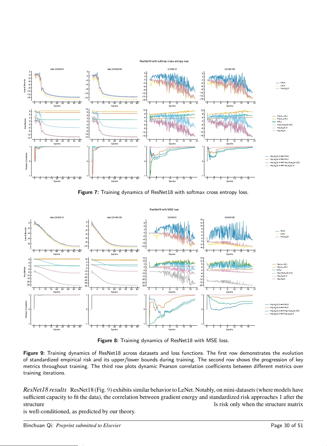
Conjugate Lear ning Theor y: Unco v er ing t he Mechanisms of T rainability and Generalization in Deep Neural Ne tw orks Binchuan Qi a,b , ∗ ,1 a T ongji Univ ersity, Siping Street, 200092 Shanghai, China b Zhejiang Y uying Colleg e of V ocational T ec hnology, Sihao Stree t, Hangzhou, 310018, Zhejiang, China A R T I C L E I N F O Keyw ords : conv ex conjugate duality learning theory non-conv ex optimization generalization bounds deep lear ning A B S T R A C T Machine lear ning techniques centered on deep neural networks (DNNs) hav e achiev ed remark - able empirical success across a broad spectrum of domains, ranging from computer vision and natural languag e processing to reinf orcement learning. Howe ver, owing to t he inherent complexity and arc hitectural diversity of modern DNNs, two fundamental challenges remain insuﬃciently addressed within the scope of classical lear ning theor y: trainability, which concer ns why simple gradient-based iterative optimization algorithms can eﬀectively optimize highly non-conv ex DNN models to achie ve low empir ical r isk, and generalization, which explains how over -parameterized DNNs consistently attain strong generalization per f or mance on un- seen data despite possessing far more parameters than training samples. In this w ork, we propose a notion of practical learnability grounded in ﬁnite sample settings, and dev elop a conjugate learning theoretical framewor k based on con vex conjugate duality to characterize this lear nability property . Building on this foundation, we demonstrate that training DNNs with mini-batch s tochastic gradient descent (SGD) ac hieves global optimality of empirical risk by jointly controlling the extremal eigenv alues of a structure matrix and the gradient energy , and we establish a cor responding con vergence theorem. We further elucidate the impact of batch size and model architecture (including depth, parameter count, sparsity , skip connections, and other characteristics) on non-conve x optimization. Additionall y , we der ive a model-agnostic low er bound for the achie vable empirical risk , theoretically demonstrating t hat data deter mines the fundamental limit of trainability . On the generalization front, we derive deterministic and probabilistic bounds on generalization er ror based on generalized conditional entropy measures. The f or mer explicitl y delineates the range of generalization er ror , while the latter characterizes the distribution of generalization er ror relative to the deterministic bounds under independent and identically distr ibuted (i.i.d.) sampling conditions. Furthermore, these bounds e xplicitly quantify the inﬂuence of three key factors: (i) inf or mation loss induced by ir rev ersibility in the model, (ii) t he maximum attainable loss value, and (iii) t he generalized conditional entropy of features with respect to labels. Moreov er, they oﬀer a uniﬁed theoretical lens f or understanding the roles of regular ization, irreversible transformations, and network depth in shaping the generalization beha vior of deep neural netw orks. Finall y , we validate our theoretical predictions through extensiv e deep lear ning experiments. The close alignment between theory and empir ical results conﬁrms the cor rectness of t he proposed framew ork. 1. Introduction Machine lear ning tec hniques based on deep neural netw orks (DNNs) hav e achie ved unprecedented empirical suc- cess across a broad spectr um of real-world applications, including imag e classiﬁcation, natural language underst anding, speech recognition, and autonomous dr iving. Despite this widespread practical success, the theoretical foundations underpinning the trainability (t he ability to optimize non-conv ex models to low empir ical r isk) and g eneralization (the ability to per f or m well on unseen data) of DNNs remain poorly understood. As a result, deep lear ning is often characterized as an experiment al science, wit h theoretical developments lagging behind practical adv ances and oﬀering limited actionable guidance f or real-world model design, algor ithm selection, and hyperparameter tuning. In this work, we propose the conjugate lear ning theory framew ork to systematicall y analyze the optimization dynamics and generalization mechanisms that under pin the per formance of deep neural networ ks in practical learning scenarios. 2080068@tongji.edu.cn (B. Qi) OR CID (s): 0000-0001-5832-1884 (B. Qi) Binchuan Qi: Pr epr int submitted to Elsevier Page 1 of 51 Conjugate Learning Theory 1.1. The trainability puzzle The trainability of DNNs ref ers to t he well-documented empir ical obser vation that highly ov er-parame ter ized, non-con ve x DNN models, when optimized wit h simple ﬁrst-order optimization methods such as stochastic gradient descent (SGD) and its variants, consistently conv erge to high-quality solutions wit h low empir ical r isk, despite the absence of con ve xity or strong regular ity assumptions that are typically required for theoretical guarantees in classical optimization [ 50 ]. In contrast, classical non-conv ex optimization theor y only guarantees con ver gence to stationar y points (points where the g radient is zero), which may cor respond to local minima, saddle points, or maxima [ 22 ], and ev en seemingly simple non-conv ex optimization problems (e.g., quadratic programming with non-conv ex constraints or copositivity testing) are prov en to be NP-hard in the general case [ 31 ]. This fundament al disconnect means that the remarkable practical eﬃciency of SGD in training DNNs cannot be explained by classical optimization t heory , highlighting the need f or new theoretical frame works tailored to the unique properties of DNNs. Sev eral theoretical directions ha ve emerg ed in recent years to address this trainability puzzle. One prominent line of work focuses on t he inﬁnite-width limit of DNNs, leading to the dev elopment of t he Neural Tang ent Kernel (NTK) framew ork [ 21 ], which provides valuable insights into the training dynamics of DNNs in the lazy training regime (where netw ork parameters chang e minimally dur ing training). Another complementar y direction, based on Fenchel- Y oung losses, establishes a direct link between gradient norms and distribution ﬁtting er rors in supervised classiﬁcation tasks [ 35 ]. How ev er, as we detail in Section 7 , t hese exis ting approac hes ha ve signiﬁcant limitations: NTK theor y struggles to capture the training dynamics of ﬁnite-width DNNs (the setting of practical interest), while t he Fenchel- Y oung perspective is restr icted to classiﬁcation tasks and does not address the generalization proper ties of DNNs. 1.2. The generalization paradox Gener alization refers to the ability of DNN models to make accurate predictions on unseen test data after being trained on a ﬁnite set of training samples. Classical statistical lear ning theor y quantiﬁes generalization per f or mance by der iving upper bounds on generalization er ror (the diﬀerence between test and training er ror) using complexity measures of the hypothesis class, such as VC-dimension [ 44 ] or Rademacher complexity [ 4 ]. These classical bounds universall y sugges t that controlling t he size and comple xity of the model promotes better generalization per f or mance, as more complex models are more prone to ov er ﬁtting to noise in t he training dat a. How ever , in the ov er-parame ter ized regime, where DNNs often contain orders of magnitude more parameters than training samples, these classical bounds f ail to reﬂect the str ong empirical gener alization performance observed in practice, a phenomenon known as the generalization paradox of DNNs. T o explain this parado x, sev eral alternative theoretical framew orks hav e been proposed in t he literature. The ﬂat minima hypo t hesis posits that the inherent stochasticity of SGD acts as an implicit regular izer dur ing training, steering t he optimization process tow ard ﬂat regions of t he loss landscape (minima wit h low curvature) that are empir ically associated with better generalization [ 23 , 10 ]. Inf or mation-theoretic approaches, most notably the Inf or mation Bottleneck (IB) pr inciple, explain generalization t hrough the lens of information compression in neural representations, arguing that DNNs lear n to retain only t he input information relev ant for predicting t arg et labels while discarding redundant or noisy components [ 41 , 39 ]. Y et as we discuss in Section 7 , each of these perspectives has its own critical limitations: ﬂatness measures are not inv ar iant to network parameterization [ 15 ] (meaning identical prediction functions can exhibit drastically diﬀerent ﬂatness values under diﬀerent parameterizations), and IB t heory f aces signiﬁcant practical challeng es in estimating mutual inf or mation in high-dimensional neural representation spaces. 1.3. T ow ard a uniﬁed framew ork Cur rent empir ical evidence and theoretical studies collectiv ely suggest that the trainability and g eneralization of DNNs are inﬂuenced by multiple interrelated factors, including t ask type (classiﬁcation, reg ression), intrinsic data characteristics (distribution, noise), model architectural design (dept h, widt h, skip connections), optimization algorit hm choices (batch size, lear ning rate), and loss function design. Existing theoretical approaches typically focus on only one or a small subset of these factors, making it diﬃcult to oﬀer a uniﬁed and comprehensiv e perspective on the behavior of DNNs in practical learning scenarios. Given these limitations of existing frame works, there is an urg ent need f or a new theoretical foundation that uniﬁes t he analysis of trainability and generalization under a single coherent framew ork, while accounting f or the inter play between key inﬂuencing factors. Our key insight that addresses this gap is that all practical machine lear ning t asks can be fundamentally viewed as problems of conditional distr ibution estimation: lear ning the conditional distribution of a targe t variable given input Binchuan Qi: Pr epr int submitted to Elsevier P age 2 of 51 Conjugate Learning Theory f eatures from a ﬁnite set of training samples. Building on this core insight, we dev elop conjugate lear ning theor y through three logically connected steps: 1. Conditional distribution view : W e f or mally argue that any practicall y learnable task inherently inv olv es estimating t he conditional distr ibution of a t arg et variable 𝑌 giv en input f eatures 𝑋 , rather than merely ﬁtting a deterministic function from 𝑋 to 𝑌 . 2. Exponential family necessity : By the Pitman–Dar mois–Koopmans theorem [ 34 , 24 , 14 ], when t he suppor t of the targe t distribution is known a pr iori, the only families of distr ibutions that can be consistently estimated from ﬁnite samples are exponential families. This fundamental result leads to a notion we ter m practical lear nability , which deﬁnes the set of task s t hat can be eﬀectiv ely sol ved with limited training data. 3. F enchel- Y oung loss : W e prov e that maximum lik elihood estimation of exponential famil y distributions is equiv alent to minimizing a Fenchel- Y oung loss function, which thus becomes the mathematical cor nerstone of our conjugate lear ning framew ork. In this uniﬁed framew ork, all learning t asks are formalized as problems of estimating a measurable mapping between random variables representing input features and output t arg ets, based on a ﬁnite sampled dat aset (not necessar il y i.i.d.), domain-speciﬁc pr ior know ledge encoded as conv ex constraints, and a con ve x conjugate dual space deﬁned ov er a well-speciﬁed hypothesis space of DNN models. 1.4. Main contr ibutions Our main contributions to t he t heoretical understanding of DNNs are as follo ws (with cor responding sections indicated f or reference): 1. W e propose conjugat e lear ning theor y , a nov el and comprehensive theoretical framew ork for modeling machine learning tasks based on DNNs. Within this framew ork, div erse learning tasks (classiﬁcation, regression, generativ e modeling) are uniﬁed under a common mat hematical formalization that lev erages conv ex conjugate duality . (Section 3 ) 2. W e establish a fundament al result that the Fenchel–Y oung loss is t he unique admissible form of the loss function under mild regularity conditions (continuity , diﬀerentiability , and consistency with maximum likelihood estimation), and provide a pr incipled methodology for designing task-speciﬁc loss functions by incor porating domain-speciﬁc prior know ledge as con ve x constraints. (Section 3 ) 3. W e introduce a nov el structure matrix to quantitativel y characterize the trainability of DNNs induced by model architectural f eatures. W e prov e a ke y equivalence result: the optimization of the non-conv ex empirical r isk loss for DNNs can be equiv alently understood as the problem of minimizing gradient energy (a measure of optimization progress) while controlling the extremal eigenv alues of t he structure matrix (which capture t he spectral properties of the model). (Section 4 ) 4. W e deﬁne a gr adient corr elation factor that quantiﬁes the joint inﬂuence of dat a properties, batch size, and model architecture on the conv ergence rate of mini-batch SGD. Based on this f actor, we establish a rigorous conv ergence theorem that bounds the rate of empir ical risk reduction for mini-batch SGD in the conjugate lear ning frame work. (Section 4 ) 5. W e use gener alized conditional entrop y to der iv e both deter ministic and probabilistic bounds on generalization er ror for DNNs. These bounds explicitly quantify t he impact of three key factors on generalization per f or mance: inf or mation loss from ir re versible model operations, loss function scale, and intrinsic data characteristics. (Section 5 ) 6. W e validate the core theoretical predictions on trainability and gener alization through extensiv e controlled experiments on benchmar k datasets and standard DNN architectures. The experimental results demonstrate strong quantitative alignment with both our t heoretical predictions and ke y ﬁndings from existing theoretical w ork. (Section 6 ) 1.5. Paper organization The rest of the paper is or ganized as f ollow s: Section 7 surve ys related work in detail. Section 2 introduces fundamental concepts and key lemmas. Section 3 presents the conjug ate lear ning framew ork (Contr ibutions 1-2). Section 4 analyzes trainability through the str ucture matrix and gradient cor relation f actor (Contr ibutions 3-4). Section 5 establishes generalization bounds based on generalized conditional entropy (Contribution 5). Section 6 validates all theoretical predictions experiment all y (Contribution 6). All technical proofs of theorems, lemmas, and corollaries are provided in full detail in the Appendix. Binchuan Qi: Pr epr int submitted to Elsevier P age 3 of 51 Conjugate Learning Theory 2. Preliminaries This section establishes the f oundational concepts and notation used throughout the paper . Subsection 2.1 introduces the basic notation for probability , dat a, models, and conv ex analy sis. Subsection 2.2 presents suppor ting lemmas from con ve x analysis and information theor y t hat will be used in later proofs. 2.1. Notation 2.1.1. Basic probability not ation • The random pair 𝑍 = ( 𝑋 , 𝑌 ) follo ws t he distr ibution 𝑞   (abbreviated as 𝑞 ) and t akes values in t he product space  =  ×  , where  denotes the input f eature space and  is a ﬁnite set of t arg ets (labels). The cardinality of  is denoted by    . Throughout this paper, we assume t hat    is ﬁnite, a condition that aligns with practical machine lear ning scenarios. • For clarity and conciseness, we represent distr ibution functions in v ector form: 𝑞  ∶=  𝑞 𝑍 ( 𝑧 1 ) , … , 𝑞 𝑍 ( 𝑧    )  ⊤ , 𝑞  ∶=  𝑞 𝑋 ( 𝑥 1 ) , … , 𝑞 𝑋 ( 𝑥    )  ⊤ , 𝑞   𝑥 ∶=  𝑞 𝑌  𝑋 ( 𝑦 1  𝑥 ) , … , 𝑞 𝑌  𝑋 ( 𝑦     𝑥 )  ⊤ , (1) where 𝑞 𝑋 ( ⋅ ) and 𝑞 𝑌  𝑋 ( ⋅  ⋅ ) denote the marginal and conditional probability mass functions (PMFs), respectiv ely . In this paper, we use 𝑞  , 𝑞  , and 𝑞   𝑥 to denote t he vectorized forms of 𝑞 𝑍 ( ⋅ ) , 𝑞 𝑋 ( ⋅ ) , and 𝑞 𝑌  𝑋 ( ⋅  𝑥 ) , respectivel y . The conditional distribution 𝑞   𝑋 is treated as a function parameterized by 𝑋 , denoted as 𝑞  ( 𝑥 ) . • Let 𝛿 𝑍 denote t he random variable obtained by mapping elements of  to    -dimensional one-hot vectors; w e ref er to this as the index representation of 𝑍 . • For a giv en input 𝑥 ∈  , deﬁne the conditional mean of 𝑌 as  𝑌  𝑥 ∶=  𝑦 ∈  𝑞   𝑥 ( 𝑦 ) 𝑦 . The quantity  𝑌  𝑋 is thus a random variable that depends on the input random variable 𝑋 . 2.1.2. Data and empir ical distr ibution • The sample dataset is denoted by the 𝑛 -tuple 𝑠 𝑛 ∶= { 𝑧 ( 𝑖 ) } 𝑛 𝑖 =1 = {( 𝑥 ( 𝑖 ) , 𝑦 ( 𝑖 ) )} 𝑛 𝑖 =1 , where each pair ( 𝑥 ( 𝑖 ) , 𝑦 ( 𝑖 ) ) is dra wn from the unknown tr ue joint distr ibution 𝑞   (abbreviated as 𝑞 ), and 𝑛 is t he total number of samples. • Let  𝑞 𝑛  (abbreviated as  𝑞 ) denote the empir ical distribution induced by 𝑠 𝑛 , deﬁned as  𝑞 ( 𝑧 ) ∶= 1 𝑛 𝑛  𝑖 =1 𝟏 { 𝑧 ( 𝑖 ) } ( 𝑧 ) , (2) f or all 𝑧 ∈  ×  . • W e deﬁne an auxiliar y random variable 𝑍 ′ = ( 𝑋 ′ , 𝑌 ′ ) t hat follo ws the empirical distr ibution  𝑞 , i.e., 𝑍 ′ ∼  𝑞 . This probabilistic representation enables us to treat the ﬁnite training dat aset 𝑠 𝑛 as a realization of a well-deﬁned distribution  𝑞 , while ensur ing all realizations of 𝑍 ′ remain within the product space  ×  . 2.1.3. Model and function space • W e use 𝑓 𝜃 ( 𝑥 ) (of ten abbreviated as 𝑓 ( 𝑥 ) ) to denote a model parameterized by 𝜃 e valuated at input 𝑥 . The function (hypothesis) space associated with input 𝑥 is deﬁned as  Θ ( 𝑥 ) ∶= { 𝑓 𝜃 ( 𝑥 ) ∶ 𝜃 ∈ Θ} . Deﬁne  ( 𝑋 ) = { 𝑓 ( 𝑋 )  𝑓 ∈  } as the set of random variables induced by  and 𝑋 . This paper f ocuses on theoretical mechanisms of deep learning. Unless otherwise speciﬁed, the function space referred to in t his work is the space of functions representable by neural networ k models. Binchuan Qi: Pr epr int submitted to Elsevier P age 4 of 51 Conjugate Learning Theory 2.1.4. Conv ex analysis not ation • The indicator function of a con ve x set 𝑆 is deﬁned as 𝐼 𝑆 ( 𝑥 ) =  0 , if 𝑥 ∈ 𝑆 , +∞ , otherwise . (3) • The con ve x conjugate (Legendre–Fenc hel conjugate) of a function Φ is deﬁned as Φ ∗ ( 𝜈 ) ∶= sup 𝜇 ∈dom(Φ)   𝜇 , 𝜈  − Φ( 𝜇 )  , (4) where  ⋅ , ⋅  denotes t he standard inner product [ 42 ]. When Φ is str ictly conv ex and diﬀerentiable, its gradient with respect to 𝜇 is denoted by ∇Φ( 𝜇 ) . W e deﬁne the conjug ate dual of 𝜇 with respect to Φ as 𝜇 ∗ Φ ∶= ∇Φ( 𝜇 ) . When Φ( ⋅ ) = 1 2  ⋅  2 2 , we hav e 𝜇 ∗ Φ = 𝜇 . • The Fenchel–Y oung loss induced b y a conv ex function Φ is deﬁned as 𝑑 Φ ( 𝜇 , 𝜈 ) ∶= Φ( 𝜇 ) + Φ ∗ ( 𝜈 ) −  𝜇, 𝜈  , (5) where 𝜇 ∈ dom(Φ) and 𝜈 ∈ dom(Φ ∗ ) [ 8 ]. This f or mulation pla ys a central role in our analysis. • For a strictly conv ex function Φ , t he Bregman diverg ence is denoted by 𝐵 Φ ( 𝑦, 𝑥 ) . 2.1.5. Generalized entropy and gener alized relativ e entropy • The g eneralized entropy of a random variable 𝑌 with respect to a conv ex function Φ is deﬁned as [ 9 ] Ent Φ ( 𝑌 ) ∶= 𝔼 𝑌 [Φ( 𝑌 )] − Φ(  𝑌 ) , (6) where  𝑌 ∶= 𝔼 [ 𝑌 ] . By Jensen ’ s inequality , Ent Φ ( 𝑌 ) ≥ 0 , with equality if and only if 𝑌 is almost surely constant (pro vided Φ is str ictl y conv ex). • Let  𝑌  𝑥 ∶= 𝔼 𝑌 ∼ 𝑞   𝑥 [ 𝑌 ] denote the conditional mean of 𝑌 given 𝑋 = 𝑥 . The g eneralized conditional entropy of 𝑌 giv en 𝑋 is deﬁned as Ent Φ ( 𝑌  𝑋 ) ∶= 𝔼 𝑋  Ent Φ ( 𝑌  𝑋 = 𝑥 )  = 𝔼 𝑋 ,𝑌 [Φ( 𝑌 )] − 𝔼 𝑋  Φ(  𝑌  𝑋 )  . (7) This scalar quantity captures the expected residual uncer tainty in 𝑌 after obser ving 𝑋 , measured t hrough the lens of the con vex potential Φ . 2.1.6. Matrix notation and nor ms • The maximum and minimum eigen values of a matr ix 𝐴 are denoted by 𝜆 max ( 𝐴 ) and 𝜆 min ( 𝐴 ) , respectivel y . For a strictly con ve x function Φ , we denote t he largest and smallest eigen values of its Hessian matr ix ∇ 2 Φ( 𝑧 ) by 𝜆 max ( 𝐻 Φ ( 𝜃 )) and 𝜆 min ( 𝐻 Φ ( 𝜃 )) , respectivel y . • For an y matr ix 𝐴 ∈ ℝ 𝑚 × 𝑛 , its Frobenius nor m is deﬁned as  𝐴  𝐹 =  𝑚  𝑖 =1 𝑛  𝑗 =1  𝑎 𝑖𝑗  2  1∕2 =  t r ( 𝐴 ⊤ 𝐴 ) . It corresponds to t he Euclidean nor m of the vector formed by all entr ies of 𝐴 . 2.2. Supporting Lemmas 2.2.1. Statistical F oundations Theorem 1 (Suﬃciency Pr inciple). If 𝑇 ( 𝐗 ) is a suﬃcient statistic of 𝜃 , then any inf erence about 𝜃 should depend on the sample 𝐗 only through the value 𝑇 ( 𝐗 ) . That is, if 𝐱 and 𝐲 are two sample points such that 𝑇 ( 𝐱 ) = 𝑇 ( 𝐲 ) , then the infer ence about 𝜃 should be the same whether 𝐗 = 𝐱 or 𝐗 = 𝐲 is obser ved [ 3 ]. Theorem 2 (Pitman–Dar mois–K oopmans). Among families of pr obability distributions whose domain does not var y with the par ameter being estimated, suﬃcient statistics with bounded dimensionality (i.e., not gr owing with 𝑛 ) exist only for distributions in the exponential famil y [ 34 , 24 , 14 ]. Binchuan Qi: Pr epr int submitted to Elsevier P age 5 of 51 Conjugate Learning Theory 2.2.2. Conv ex Analysis Lemma 3 (Properties of Con vex Conjugate Duality). F or all 𝜇 , 𝜈 ∈ ℝ 𝑘 , the follo wing hold: 1. F enchel–Y oung inequality [ 42 , Proposition 3.3.4]: Φ( 𝜇 ) + Φ ∗ ( 𝜈 ) ≥  𝜇 , 𝜈  , ∀ 𝜇 ∈ dom(Φ) , 𝜈 ∈ dom(Φ ∗ ) . (8) Equality holds if and only if 𝜈 ∈ 𝜕 Φ( 𝜇 ) . If, fur thermore, Φ is strictly convex and diﬀerentiable, then equality holds iﬀ 𝜈 = 𝜇 ∗ Φ . 2. Let Φ = Ψ + 𝐼 𝐶 . Then [ 5 ] Φ ∗ ( 𝜈 ) = inf 𝜈 1 ∈ ℝ 𝑑  𝜎 𝐶 ( 𝜈 1 ) + Ψ ∗ ( 𝜈 − 𝜈 1 )  , (9) wher e 𝜎 𝐶 ( 𝜈 ) = sup 𝑦 ∈ 𝐶  𝜈 , 𝑦  is the suppor t function of 𝐶 (i.e., 𝐼 ∗ 𝐶 = 𝜎 𝐶 ). 3. If Φ is strictly conve x and diﬀerentiable, then Φ ∗ is also strictly convex and diﬀerentiable, and 𝜈 ∗ Φ ∈ dom(Φ) for all 𝜈 ∈ dom(Φ ∗ ) [ 42 ]. 4. Addition to aﬃne function If 𝑓 ( 𝑥 ) = 𝑔 ( 𝑥 ) + 𝑎 𝑇 𝑥 + 𝑏 , then 𝑓 ∗ ( 𝑦 ) = 𝑔 ∗ ( 𝑦 − 𝑎 ) − 𝑏 [ 42 ]. 2.2.3. Properties of F enchel- Y oung Losses Lemma 4 (Properties of F enchel–Y oung Losses [ 8 ]). 1. Non-neg ativity. 𝑑 Φ ( 𝜇 , 𝜈 ) ≥ 0 for any 𝜇 ∈ dom(Φ) and 𝜈 ∈ dom(Φ ∗ ) . If Φ is a proper , lower semi-continuous, conv ex function, then 𝑑 Φ ( 𝜇 , 𝜈 ) = 0 if and only if 𝜈 ∈ 𝜕 Φ( 𝜇 ) . If Φ is str ictly conve x and diﬀerentiable, then 𝑑 Φ ( 𝜇 , 𝜈 ) = 0 iﬀ 𝜈 = 𝜇 ∗ Φ . 2. Diﬀerentiability . If Φ is strictly conve x and diﬀerentiable, then 𝑑 Φ ( 𝜇 , 𝜈 ) is diﬀer entiable in both arguments. In particular , ∇ 𝜈 𝑑 Φ ( 𝜇 , 𝜈 ) = 𝜈 ∗ Φ ∗ − 𝜇 . 3. Relation to Bregman diverg ences. Let 𝜈 = 𝜇 ∗ Φ (i.e., ( 𝜇 , 𝜈 ) form a dual pair), where Φ is strictly conv ex. Then the Bregman diver gence satisﬁes 𝐵 Φ ( 𝑦  𝜇 ) = 𝑑 Φ ( 𝑦, 𝜈 ) . Thus, F enchel–Y oung losses can be viewed as a “mixed- form” Br egman diver gence [ 1 , Theorem 1.1], where the second argument is expr essed in dual coor dinates. 2.2.4. Information- Theoretic Inequalities Lemma 5 (KL Div ergence Upper Bound). If 𝑝 and 𝑞 are probability densities/masses both suppor ted on a bounded interval 𝐼 , then we have [ 13 ] 𝐷 KL ( 𝑝, 𝑞 ) ≤ 1 inf 𝑥 ∈ 𝐼 𝑞 ( 𝑥 )  𝑝 − 𝑞  2 2 . (10) Lemma 6 (Pinsk er’s Inequality [ 12 ]). If 𝑝 and 𝑞 ar e probability densities/masses both supported on a bounded interval 𝐼 , then we have 𝐷 𝐾 𝐿 ( 𝑝  𝑞 ) ≥ 1 2 ln 2  𝑝 − 𝑞  2 1 . (11) 3. Conjugate learning frame wor k In this section, we f or malize t he machine lear ning task and derive the conjugate lear ning framew ork. W e argue that conjugate learning arises not merely as a con venient modeling choice, but as a necessar y consequence of fundament al statistical pr inciples gov er ning learnability from ﬁnite dat a. Subsection 3.1 establishes t he practical lear nability of exponential families. Subsection 3.2 presents the f or mal deﬁnition of conjugate lear ning. Subsection 3.3 elaborates on its three core components. Subsection 3.4 introduces key quantities for analyzing trainability and generalization. 3.1. Practical learnability and exponential families A general machine learning problem can be view ed as using obser ved samples to train a model that accurately predicts a t arg et variable given input f eatures. From a probabilistic perspective, this is equiv alent to estimating the conditional distr ibution 𝑝   𝑥 of the t ar get 𝑦 given the feature 𝑥 , based on a ﬁnite dataset. When framing lear ning as conditional distribution estimation, tw o key obser vations emerge: Binchuan Qi: Pr epr int submitted to Elsevier P age 6 of 51 Conjugate Learning Theory 1. The suppor t (i.e., the set of possible values) of the target distribution is typically known a priori and independent of the distribution’ s parameters. For example, classiﬁcation tasks hav e t arg ets in a ﬁnite label set {1 , … , 𝐾 } , while regression tasks ha ve targ ets in ℝ 𝑑 , both of which are ﬁxed regardless of the conditional distribution parameters. 2. Due to t he suﬃciency pr inciple, parametr ic statistical inf erence must be based on suﬃcient statistics. To ﬁt and learn the underlying data distr ibution using a model with a ﬁnite number of parameters, t he suﬃcient statistics of the distribution must be ﬁnite-dimensional and must not grow with the sample size 𝑛 . In the absence of additional structural assumptions or pr ior kno wledg e, accurately lear ning the conditional probability distribution from ﬁnite samples requires that t he distribution admit ﬁnite-dimensional suﬃcient statistics. The second observation is critical: inﬁnite-dimensional suﬃcient statistics cannot be fully determined from a ﬁnite number of samples, making consistent estimation impossible. This limitation is r igorousl y c haracter ized by the Pitman–Darmois–Koopmans theorem, which states that among all parametric families with ﬁxed suppor t, only exponential famil y distributions possess suﬃcient statistics whose dimension remains bounded as t he sample size 𝑛 → ∞ . Consequently , exponential families are t he only distributions t hat are practically learnable from ﬁnite samples using ﬁnite-capacity parametric models. Proposition 7 (Practical Learnability). In the absence of additional structural assumptions or prior know ledge, onl y distributions in the e xponential family ar e pr actically learnable fr om ﬁnite samples using parame tr ic models in mac hine learning. Common ex amples of exponential-f amily distr ibutions include the Gaussian, categor ical, binomial, multinomial, Poisson, Gamma, Beta, and chi-sq uared distr ibutions. In contrast, notable non-exponential-f amily distributions include the unif or m, Cauch y , Laplace, W eibull, extreme-v alue, and hyperg eometr ic distr ibutions, as well as location-scale f amilies without ﬁxed support. While real-w orld data may follo w non-e xponential-famil y la w s, the y can often be eﬀectivel y appro ximated within t he exponential-f amily framew ork. Speciﬁcally , under i.i.d. sampling, any distr ibution ov er a bounded domain can be approximated arbitrar ily well by a discrete distr ibution with ﬁnite suppor t. The joint distribution of 𝑛 independent samples from suc h a discrete distr ibution is exactl y multinomial, a member of the exponential famil y . Therefore, by discr etizing the targ et space ﬁnely enough, any learning task can be reduced to estimating a multinomial (or categorical) conditional distribution with controllable appr oximation err or . This justiﬁes the use of exponential-f amily modeling as a universal paradigm for practical machine learning. 3.2. F ormal deﬁnition of conjugate learning 3.2.1. Derivation from exponential families Building on the practical lear nability of exponential famil y distributions, we focus on modeling the conditional probability distribution of t he label 𝑦 given t he f eature 𝑥 under the exponential famil y assumption. W e parameterize the conditional distribution as an exponential f amily with natural parameters dependent on the input features: 𝑞   𝑥 ( 𝑦 ) = ℎ ( 𝑦 ) exp  𝑦 ⊤ 𝜂 𝑥 − 𝐵 ( 𝜂 𝑥 )  , (12) where 𝐵 ( 𝜂 𝑥 ) = log  𝑦 ∈  ℎ ( 𝑦 ) exp{ 𝑦 ⊤ 𝜂 𝑥 } is t he cumulant function (also kno wn as the log-par tition function). Under mild regularity conditions (e.g., the support of 𝑦 is ﬁxed and ℎ ( 𝑦 ) > 0 ), t he cumulant function 𝐵 is strictly con ve x in 𝜂 𝑥 . Thus, our lear ning objective is to estimate t he natural parameter 𝜂 𝑥 using a parametric model 𝑓 𝜃 ( 𝑥 ) , where 𝜃 denotes the model parameters. The distr ibution predicted by the model is expressed as: 𝑝   𝑥 ( 𝑦 ) = exp  − 𝑑 Ω ( 𝑦, 𝑓 𝜃 ( 𝑥 )) + log ℎ ( 𝑦 ) + log Ω( 𝑦 )  , (13) where Ω = 𝐵 ∗ denotes the con ve x conjugate of 𝐵 . The negativ e log-likelihood becomes 𝓁 ( 𝜃 ; 𝑠 ) ∝  ( 𝑥,𝑦 )∈ 𝑠 𝑑 Ω ( 𝑦, 𝑓 𝜃 ( 𝑥 )) . (14) This result show s that maximum likelihood estimation under an exponential-f amily model is equivalent to minimizing the sum of Fenchel–Y oung losses betw een t he t arg et 𝑦 and the model output 𝑓 𝜃 ( 𝑥 ) . Binchuan Qi: Pr epr int submitted to Elsevier P age 7 of 51 Conjugate Learning Theory 3.2.2. The conjugate learning objective Deﬁnition 1 (Conjugate Learning). Given a sample dataset 𝑠 𝑛 , sample spaces  and  , pr ior know ledge encoded as a conv ex set 𝐶 ⊆ ℝ 𝑑 containing all f easible targe t values, a model space  Θ = { 𝑓 𝜃 ∶ 𝜃 ∈ Θ} , and a diﬀerentiable strictly conv ex function Ω (the g enerating function ), t he conjugate lear ning task is to solv e min 𝜃 ∈Θ 𝔼 𝑋 ,𝑌  𝑑 Φ ( 𝑌 , 𝑓 𝜃 ( 𝑋 ) ∗ Φ ∗ )  , (15) where Φ( ⋅ ) = Ω( ⋅ ) + 𝐼 𝐶 ( ⋅ ) , 𝐼 𝐶 is the indicator function of 𝐶 , 𝑓 𝜃 ( 𝑋 ) ∗ Φ ∗ denotes the conjugate dual of 𝑓 𝜃 ( 𝑋 ) with respect to Φ , and  is a ﬁnite set (justiﬁed by discretization of continuous features in practice). 3.2.3. Key featur es The conjugate lear ning framew ork diﬀers from the classical f or mulation in the f ollowing ke y aspects: 1. Relax ed i.i.d. assumption : The framew ork does not require samples to be str ictl y i.i.d., accommodating realistic scenarios such as dat a augmentation and sequential dependencies in natural language or time-ser ies data. In practical machine lear ning, training data frequentl y deviates from t he i.i.d. assumption due to factors such as data augment ation (e.g., Mixup [ 52 ] in f ew-sho t learning) or inherent sequential cor relations in context-label pairs (e.g., natural language modeling). The conjugate lear ning framewor k is designed to handle such non-i.i.d. data distributions while retaining the ability to conduct theoretical analysis under t he i.i.d. sampling regime as a special case. 2. Explicit prior integration : Pr ior know ledge is encoded through the conv ex constraint set 𝐶 , which guides the learning process by restr icting the feasible region of predictions. This extends classical lear ning settings where prior information is either implicitly embedded in the model architecture or completely ignored. By encoding domain-speciﬁc or t ask -speciﬁc prior kno w ledge into t he con ve x set 𝐶 , the framew ork lev erages str uctured prior information to improv e generalization performance on complex t asks and reduce the hypo t hesis space complexity to accelerate optimization. 3. Conjugate dual prediction : The ﬁnal prediction is deﬁned as the conjugate dual of the ra w model output, ensuring structural alignment with the t arg et space. Unlik e classical framew orks t hat use the ra w model output 𝑓 𝜃 ( 𝑥 ) directly for prediction, conjugate lear ning uses 𝑓 𝜃 ( 𝑥 ) ∗ Φ ∗ (the conjugate dual of 𝑓 𝜃 ( 𝑥 ) wit h respect to Φ ) as the ﬁnal prediction. This design imposes meaningful str uctural constraints on the prediction space that align with the proper ties of the targe t distr ibution (e.g., probability simplex f or classiﬁcation). 4. F enchel- Y oung loss famil y : The loss function is constrained to t he Fenc hel- Y oung famil y , whic h includes common losses like cross entropy and MSE. Unlike arbitrar y loss functions adopted in classical learning framew orks, Fenchel–Y oung losses possess well-deﬁned str uctural properties t hat we demonstrate to play a piv otal role in ensur ing both the trainability and generalization of the model in subsequent sections. 5. Finite feature space : The input feature space  is assumed to be ﬁnite, a condition justiﬁed by the discretization of continuous features in practical lear ning scenar ios. While the label space  can be inﬁnite-dimensional (e.g., regression in ℝ 𝑑 ), the f eature space  is required to be ﬁnite. This assumption aligns wit h core learnability theor y: consistent lear ning in continuous f eature spaces is only possible when t he space admits an eﬀective discretization (e.g., via ﬁnite-resolution binning). Ot herwise, if arbitrar ily nearb y inputs may exhibit arbitrarily diver gent label distributions, the task becomes fundament all y unlear nable by any model of ﬁnite capacity . Figure 1 illustrates the architecture and processing ﬂow of t he conjugate lear ning framew ork. Starting from an input 𝑥 , the parametric model 𝑓 𝜃 produces an inter mediate output, which is mapped to its conjugate dual via t he operator ( ⋅ ) ∗ Φ ∗ . The Bregman diverg ence 𝐵 Φ ( 𝑦, 𝑓 𝜃 ( 𝑥 ) ∗ Φ ∗ ) is then computed between t his dual prediction and t he targe t 𝑦 , f or ming the optimization objectiv e. Notably , in classiﬁcation tasks, the sof tmax activ ation function and cross entropy loss cor respond precisely to ( ⋅ ) ∗ Φ ∗ and 𝐵 Φ ( 𝟏 𝑦 , ⋅ ) (respectivel y) when Φ is the negativ e Shannon entropy . In regression tasks, the mean squared er ror (MSE) loss ar ises as 𝐵 Φ ( 𝑦, ⋅ ) with Φ = 1 2  ⋅  2 2 , under which t he conjugate dual operator ( ⋅ ) ∗ Φ ∗ reduces to the identity map. Binchuan Qi: Pr epr int submitted to Elsevier P age 8 of 51 Conjugate Learning Theory Samples Model Prediction Loss function Prior knowledge Optimization algorithm Figure 1: Schematic illustration of the conjugate learning framewo rk. The diagram outlines the complete processing pip eline from raw input to lea rning target appro ximation, emphasizing the interpla y among model output, conjugate transformation, and distance measurement. Fundamentally , conjugate lear ning is a str uctured instantiation of the classical statistical lear ning framew ork. It preserves core components (training data, hypothesis space, loss function) while introducing a critical augmentation: explicit integration of prior know ledge via the con vex set 𝐶 . As shown in subsequent sections, this augmentation enhances analytical tractability and pro vides a unifying explanation for the empirical success of many deep lear ning practices. 3.3. Core components of the framew ork 3.3.1. Generating function and pr ior knowledg e If the true conditional distr ibution belongs to a known exponential famil y , its str ucture uniquely determines the generating function Ω . For e xample, the Gaussian distribution cor responds to Ω = 1 2  ⋅  2 2 , while the categorical distribution cor responds to the negativ e Shannon entropy . If the tr ue distribution does not belong to an exponential f amily , the empirical distribution can be approximated by a multinomial distribution, whose generating function is the negativ e Shannon entropy . In practical machine lear ning task s, the suppor t of the target variable 𝑌 (denoted  ) is often known or par tially characterized by pr ior know ledge. W e express this pr ior know ledge as  ⊆ 𝐶 , where 𝐶 is a conv ex set cont aining all values consistent wit h the task constraints. A canonical example is super vised classiﬁcation with 𝑚 classes: since the goal is to estimate a conditional pr obability dis tr ibution, predictions must lie in t he probability simple x Δ 𝑚 = { 𝑝 ∈ ℝ 𝑚 ∶  𝑚 𝑖 =1 𝑝 𝑖 = 1 , 𝑝 𝑖 ≥ 0} . If t he model architecture is designed such that its predictions inherently satisfy the constr aint 𝐶 , the structural mismatch between predictions and targets is eliminated. This restr icts the optimization search space, facilitating faster con verg ence of both empir ical and expected r isk. Empir ically , richer pr ior know ledge leads to a smaller f easible set 𝐶 , which reduces the hypothesis complexity and improv es lear ning eﬃciency and accuracy . The ubiquitous softmax lay er in classiﬁcation networks ex empliﬁes this principle: it maps ra w outputs from ℝ 𝑚 onto the probability simplex Δ 𝑚 , which, from the perspective of conjugate lear ning, emerges naturally as a mechanism to enforce pr ior kno wledg e and align t he model’s prediction geometry with that of the lear ning target. 3.3.2. Conjugate dual prediction As discussed in Subsection 3.3.1 , a ke y challeng e is ensuring t hat model predictions share t he structural properties of the lear ning targe t. Conjugate lear ning addresses this by le veraging duality to enf orce alignment between predictions and t he target space. Given a generating function Ω with domain dom(Ω) , deﬁne Φ = Ω + 𝐼 𝐶 , so that dom(Φ) = dom(Ω) ∩ 𝐶 . By Lemma 3 , for any 𝜈 ∈ dom(Φ ∗ ) , it holds that ∇Φ ∗ ( 𝜈 ) ∈ dom(Φ) . In t he context of Deﬁnition 1 , t he prediction obtained via dual mapping satisﬁes 𝑓 𝜃 ( 𝑥 ) ∗ Φ ∗ ∶= ∇Φ ∗ ( 𝑓 𝜃 ( 𝑥 )) ∈ dom(Φ) = dom(Ω) ∩ 𝐶 . (16) Moreov er , t he con ve x conjugate Φ ∗ admits the representation Φ ∗ ( 𝜇 ) = inf 𝜇 ′ ∈ ℝ 𝑑  𝜎 𝐶 ( 𝜇 ′ ) + Ω ∗ ( 𝜇 − 𝜇 ′ )  , (17) Binchuan Qi: Pr epr int submitted to Elsevier P age 9 of 51 Conjugate Learning Theory where 𝜎 𝐶 ( 𝜇 ) = sup 𝑞 ∈ 𝐶  𝜇 , 𝑞  is t he suppor t function of 𝐶 . Although computing Φ ∗ from Ω and 𝐶 is generally nontr ivial, many practical constraints are linear . For instance, in classiﬁcation scenarios where we expect t he prediction results to be the distribution of labels given features, the predictions lie within a probability simplex, such t hat 𝐶 = { 𝑦 ∈ ℝ 𝑑 ∶  𝑖 𝑦 𝑖 = 1 and 𝑦 𝑖 > 0} . In this case, the constraint condition is linear, and the f ollowing theorem pro vides a closed-form solution. Theorem 8. Let 𝐺 ∈ ℝ 𝑚 × 𝑑 be a matrix with r ows 𝐺 ⊤ 𝑖 , and deﬁne the constr aint set 𝐶 = { 𝑦 ∈ ℝ 𝑑 ∶ 𝐺𝑦 = 𝑏 } . Then, Φ ∗ ( 𝜈 ) = Ω ∗ ( 𝜈 + 𝐺 ⊤ 𝜆 ∗ ) −  𝜆 ∗ , 𝑏  , (18) wher e 𝜆 ∗ ∈ ℝ 𝑚 satisﬁes 𝐺 ⋅ ( 𝜈 + 𝐺 ⊤ 𝜆 ∗ ) ∗ Ω ∗ = 𝑏 . The proof is pro vided in Appendix A.1 . T o clarify theorem’ s implications, consider Ω( 𝑝 ) =  𝑖 ( 𝑝 𝑖 log 𝑝 𝑖 − 𝑝 𝑖 ) , for whic h Ω ∗ ( 𝜈 ) =  𝑖 𝑒 𝜈 𝑖 and ( 𝜈 ∗ Ω ∗ ) 𝑖 = 𝑒 𝜈 𝑖 , which does not lie in the simplex Δ 𝑚 . Imposing 𝐶 = Δ 𝑚 and setting Φ = Ω + 𝐼 𝐶 , Theorem 8 yields Φ ∗ ( 𝜈 ) = 1 +  𝑖 𝑒 𝜈 𝑖 . (19) Consequentl y , 𝜈 ∗ Φ ∗ = Sof t max( 𝜈 ) =  𝑒 𝜈 𝑖  𝑗 𝑒 𝜈 𝑗  𝑖 ∈ 𝐶 , (20) and the associated Bregman diver gence becomes 𝑑 Φ ( 𝑝, 𝜈 ) = 𝐷 K L ( 𝑝 𝜈 ∗ Φ ∗ ) . (21) This result show s that t he softmax function and cross entropy loss emerge naturally within the conjugate lear ning framew ork when Φ is the negativ e entropy regularized by the probability simplex constraint. Directly ﬁtting 𝑌 using the ra w model output 𝑓 𝜃 ( 𝑥 ) ignores av ailable prior inf or mation, leading to a larg er search space, reduced training eﬃciency , and no guarantee that predictions satisfy t he constraint 𝐶 . In contrast, conjugate lear ning provides a principled mechanism to embed pr ior kno wledg e into the learning geometry , enhancing both theoretical inter pretability and empirical per f or mance. 3.3.3. F enchel- Y oung loss as the natural loss family W e no w sho w that Fenchel–Y oung losses are not merely a conseq uence of the Pitman–Darmois–Koopmans theorem (Subsection 3.1 ) but are theoretically inevitable under natural desiderata for well-beha v ed loss functions in machine lear ning. It is well established that man y standard losses, such as cross entropy , KL diver gence, and mean squared er ror , belong to the Fenchel–Y oung f amily [ 8 ]. In machine learning, a loss function serves tw o fundament al roles: (i) quantifying discrepancy betw een predictions and targets, and (ii) guiding optimization tow ard a globall y optimal solution. A well-designed loss should therefore satisfy: 1. Strict conv exity in structured predictions : The loss 𝓁 ( 𝑦, 𝑓 𝜃 ( 𝑥 ) ∗ Φ ∗ ) must be str ictl y conv ex in t he prediction 𝑓 𝜃 ( 𝑥 ) ∗ Φ ∗ . This ensures a unique minimizer f or any ﬁxed input 𝑥 , guaranteeing t hat optimization conv erges to a well-deﬁned t arg et. Without this property , t he loss landscape ma y cont ain multiple minima, pre venting reliable con verg ence. Note that strict conv exity in the prediction does not require strict con vexity in the raw output 𝑓 𝜃 ( 𝑥 ) . 2. Properness : A loss function 𝓁 is said to be proper if the minimizer of the expected loss coincides wit h the mean of the target distribution; t hat is,  𝑌  𝑥 = ar g min 𝜈 𝔼 𝑌  𝓁 ( 𝑌 , 𝜈 )  , (22) where the e xpectation is t aken with respect to the data-generating distribution of 𝑌 giv en 𝑥 . This property ensures that the population-optimal prediction recov ers the tr ue conditional expectation of the target variable. As a consequence, the empirical risk minimizer con verg es (in probability) to  𝑌  𝑥 as the sample size grow s. Binchuan Qi: Pr epr int submitted to Elsevier P age 10 of 51 Conjugate Learning Theory Combined with the W eak La w of Large Numbers, proper ness guarantees that the empirical r isk asymptoticall y approaches the expected r isk, enabling consistent learning. Proper ness also conf ers inherent robustness to zero- mean label noise: if obser ved labels are cor r upted by additive noise wit h zero mean, the population-optimal predictor remains centered at the tr ue underl ying signal. Without proper ness, increasing the dat aset size does not guarantee conv ergence to the cor rect target. These tw o proper ties are necessary and jointly suﬃcient to character ize well-beha ved loss functions for machine learning. In fact, any diﬀerentiable loss function satisfying both pr oper ties must coincide (up to an additiv e ter m independent of the prediction) with a Fenchel–Y oung loss: Theorem 9. Let 𝓁 ( 𝑦, 𝑓 𝜃 ( 𝑥 ) ∗ Φ ∗ ) be a diﬀerentiable loss function. If 𝓁 satisﬁes both (i) str ong conv exity with respect to the model’ s pr ediction and (ii) properness, then there exists a strictly conv ex function Φ suc h that 𝓁 ( 𝑦, 𝑓 𝜃 ( 𝑥 ) ∗ Φ ∗ ) − 𝓁 ( 𝑦, 𝑦 ) = 𝑑 Φ ( 𝑦, 𝑓 𝜃 ( 𝑥 )) . (23) The proof of this theorem is given in Appendix A.2 . This result shows t hat any well-beha v ed loss function (satisfying strict con ve xity and proper ness) is equivalent to a Fenc hel–Y oung loss up to a constant oﬀset 𝓁 ( 𝑦, 𝑦 ) . Consequently , f ocusing on Fenchel–Y oung losses entails no loss of generality , providing a r igorous and widely applicable theoretical foundation for loss function choice in machine learning. As a concrete ex ample, t he sof tmax cross entropy loss satisﬁes: 𝓁 CE ( 𝑞   𝑥 , 𝑝   𝑥 ) − 𝓁 CE ( 𝑞   𝑥 , 𝑞   𝑥 ) = 𝑑 Φ  𝑞   𝑥 , 𝑓 𝜃 ( 𝑥 )  , (24) where Φ( 𝑝 ) = − 𝐻 ( 𝑝 ) is the negative entropy and 𝑝   𝑥 = Sof t max( 𝑓 𝜃 ( 𝑥 )) = 𝑓 𝜃 ( 𝑥 ) ∗ Φ ∗ . Hence, sof tmax cross entropy arises naturally as the Fenchel–Y oung loss induced b y negative entropy . 3.4. Ke y quantities for analysis 3.4.1. Risk and generalization measures W e f or mally deﬁne the e xpected risk, empirical risk, and generalization er ror within the conjugate lear ning framew ork. Deﬁnition 2 (Risk and Generalization Error). The expected risk, empir ical risk, and generalization error in conju- gate lear ning are deﬁned as  Φ ( 𝜃 , 𝑞 ) = 𝔼 𝑍 ∼ 𝑞  𝑑 Φ ( 𝑌 , 𝑓 𝜃 ( 𝑋 ))  ,  Φ ( 𝜃 ,  𝑞 ) =  Φ ( 𝜃 , 𝑠 ) = 1  𝑠   𝑧 ∈ 𝑠 𝑑 Φ ( 𝑦, 𝑓 𝜃 ( 𝑥 )) = 𝔼 𝑍 ′ ∼  𝑞  𝑑 Φ ( 𝑌 ′ , 𝑓 𝜃 ( 𝑋 ′ ))  , gen( 𝑓 𝜃 , 𝑠 𝑛 ) =     Φ ( 𝜃 , 𝑞 ) −  Φ ( 𝜃 ,  𝑞 )    , (25) where 𝑞 denotes the tr ue dat a distr ibution,  𝑞 denotes the empir ical distr ibution induced by the training set 𝑠 , and 𝑠 𝑛 denotes a training set of size 𝑛 . W e use both  Φ ( 𝜃 ,  𝑞 ) and  Φ ( 𝜃 , 𝑠 ) interc hangeably ; t he latter facilitates analy sis of mini-batch SGD. In the special case Φ( 𝑦 ) = 1 2  𝑦  2 2 , we recov er the squared 𝐿 2 loss:  𝐿 2 2 ∕2 ( 𝜃 , 𝑞 ) = 𝔼 𝑍 ∼ 𝑞  𝑌 − 𝑓 𝜃 ( 𝑋 )  2 2 . For a single sample 𝑧 = ( 𝑥, 𝑦 ) , we denote the per -sample loss by  Φ ( 𝜃 , 𝑧 ) ∶= 𝑑 Φ ( 𝑦, 𝑓 𝜃 ( 𝑥 )) . The range of the loss function varies considerably with the choice of Φ . To enable a fair compar ison of model ﬁtting per f or mance across diﬀerent loss functions, we deﬁne the standardized r isk based on the mean squared er ror betw een t he targ et and the dual prediction: Deﬁnition 3 (Standardized Expected and Empirical Risk). The standardized e xpected r isk and empir ical r isk in conjugate lear ning are deﬁned, respectivel y , as:  ◦ Φ ( 𝜃 , 𝑞 ) = 𝔼 𝑍 ∼ 𝑞  𝑌 − 𝑓 𝜃 ( 𝑋 ) ∗ Φ ∗  2 2 ,  ◦ Φ ( 𝜃 ,  𝑞 ) =  ◦ Φ ( 𝜃 , 𝑠 ) = 𝔼 𝑍 ′ ∼  𝑞  𝑌 − 𝑓 𝜃 ( 𝑋 ) ∗ Φ ∗  2 2 . (26) Binchuan Qi: Pr epr int submitted to Elsevier P age 11 of 51 Conjugate Learning Theory T o relate t he standardized risk to the general Fenc hel–Y oung loss r isk, we ﬁrst deﬁne t he extr emal eigen values of the Hessian at both the sample and dataset lev els. Deﬁnition 4 (Extremal Eigenv alues of the Model-Induced Hessian). W e deﬁne the extremal eigen values of the model-induced Hessian as 𝜆 min ( 𝐻 Φ ( 𝜃 )) ∶= inf 𝑥 ∈  𝜆 min  ∇ 2 Φ( 𝑓 𝜃 ( 𝑥 ) ∗ Φ ∗ )  , 𝜆 max ( 𝐻 Φ ( 𝜃 )) ∶= sup 𝑥 ∈  𝜆 max  ∇ 2 Φ( 𝑓 𝜃 ( 𝑥 ) ∗ Φ ∗ )  . Equiv alently , for all 𝑥 ∈  , 𝜆 min ( 𝐻 Φ ( 𝜃 )) 𝐼 ⪯ ∇ 2 Φ  𝑓 𝜃 ( 𝑥 ) ∗ Φ ∗  ⪯ 𝜆 max ( 𝐻 Φ ( 𝜃 )) 𝐼 . (27) These quantities characterize the global low er and upper bounds on t he local cur vature of Φ o ver the set of predictions generated by the model 𝑓 𝜃 on the input domain  . W e assume throughout that 0 < 𝜆 min ( 𝐻 Φ ( 𝜃 )) ≤ 𝜆 max ( 𝐻 Φ ( 𝜃 )) < ∞ , which holds for standard losses (e.g., squared er ror , logistic loss) on compact domains. The v alues 𝜆 min ( 𝐻 Φ ( 𝜃 )) and 𝜆 max ( 𝐻 Φ ( 𝜃 )) depend implicitly on the model parameters 𝜃 through t he induced predictions 𝑓 𝜃 ( 𝑥 ) ∗ Φ ∗ . For instance, when Φ is the negative Shannon entropy , i.e., Φ( 𝑝 ) =  𝑖 𝑝 𝑖 log 𝑝 𝑖 deﬁned on t he probability simplex, the Hessian ∇ 2 Φ( 𝑝 ) is diagonal with entr ies 1∕ 𝑝 𝑖 . In this case, the eigen values of ∇ 2 Φ( 𝑝 ) are precisely {1∕ 𝑝 𝑖 } 𝑘 𝑖 =1 , so t he extremal eigen values ov er a dataset cor respond to the reciprocals of the smallest and largest predicted probabilities across all classes and samples. More generall y , if the Hessian ∇ 2 Φ has unif or ml y bounded eigen values ov er its entire domain (e.g., as in the squared loss, where ∇ 2 Φ = 𝐼 ), then one may take 𝜆 min ( 𝐻 Φ ( 𝜃 )) and 𝜆 max ( 𝐻 Φ ( 𝜃 )) to be these global constants, independent of 𝜃 . Such a simpliﬁcation does not aﬀect t he validity of our theoretical conclusions, as our bounds only require the existence of ﬁnite, positive extremal cur vature constants, whether derived from t he model’ s cur rent state or from global properties of Φ . Since the general Fenchel–Y oung risk satisﬁes  Φ ( 𝜃 , 𝑧 ) = 𝑑 Φ ( 𝑦, 𝑓 𝜃 ( 𝑥 )) = 𝐵 Φ  𝑦, 𝑓 𝜃 ( 𝑥 ) ∗ Φ ∗  , by the integral form of T ay lor’ s theorem (or t he mean-value inequality for strongly conv ex functions), the Bregman diver gence admits the quadratic bound 𝜆 min ( 𝐻 Φ ( 𝜃 ))  ◦ Φ ( 𝜃 , 𝑧 ) ≤  Φ ( 𝜃 , 𝑧 ) ≤ 𝜆 max ( 𝐻 Φ ( 𝜃 ))  ◦ Φ ( 𝜃 , 𝑧 ) . (28) Consequentl y ,  Φ ( 𝜃 , 𝑧 ) and  ◦ Φ ( 𝜃 , 𝑧 ) are equiv alent up to constant factors depending only on the geometry of Φ and the cur rent model state 𝜃 . This equiv alence implies t hat minimizing one objective also minimizes the other . Ho wev er, unlike  Φ , whose scale is inherently tied to t he choice of Φ (e.g., cross entropy vs. squared loss), t he standardized risk  ◦ Φ pro vides a scale-invariant measure of prediction er ror in the pr imal space. This property makes  ◦ Φ particularly useful f or comparing optimization dynamics and generalization behavior across diﬀerent loss functions within a uniﬁed framew ork. W e deﬁne t he loss upper bound, which quantiﬁes the maximum Fenchel–Y oung loss incur red by the model ov er all inputs and targ ets: Deﬁnition 5 (Loss Upper Bound). The loss upper bound of a model 𝑓 𝜃 is deﬁned as 𝛾 Φ ( 𝜃 ) = max 𝑥 ∈  , 𝑦 ∈  𝑑 Φ  𝑦, 𝑓 𝜃 ( 𝑥 )  . (29) When Φ( 𝑝 ) =  𝑖 𝑝 𝑖 log 𝑝 𝑖 (i.e., t he negative Shannon entropy) and the task is classiﬁcation, it f ollow s fr om the deﬁnition that 𝛾 Φ ( 𝜃 ) = max 𝑥 ∈  , 𝑦 ∈  𝐷 K L  𝟏 𝑦  𝑝   𝑥  , where 𝑝   𝑥 = Sof t max( 𝑓 𝜃 ( 𝑥 )) . Consequentl y , 𝛾 Φ ( 𝜃 ) = log 1 𝑝 min , with 𝑝 min = min 𝑥 ∈  , 𝑦 ∈  𝑝   𝑥 ( 𝑦 ) . Binchuan Qi: Pr epr int submitted to Elsevier P age 12 of 51 Conjugate Learning Theory 3.4.2. Gradient-based quantities W e deﬁne gradient-based quantities that characterize the optimization dynamics of the conjugate learning framew ork: Deﬁnition 6 (Gradient Energy). For a loss function  Φ ( 𝜃 , 𝑧 ) parameterized by 𝜃 and a data distr ibution 𝑞  , the gradient energy is deﬁned as t he e xpected squared Euclidean norm of t he g radient: 𝔼 𝑍 ∼ 𝑞      ∇ 𝜃  Φ ( 𝜃 , 𝑍 )    2 2  . (30) For a single sample 𝑧 = ( 𝑥, 𝑦 ) , t he per -sample gradient energy is given by    ∇ 𝜃  Φ ( 𝜃 , 𝑧 )    2 2 . Deﬁnition 7 (Structure Matr ix). W e deﬁne the str ucture matrix associated with t he model 𝑓 𝜃 and input 𝑥 as: 𝐴 𝑥 ∶= ∇ 𝜃 𝑓 𝜃 ( 𝑥 )∇ 𝜃 𝑓 𝜃 ( 𝑥 ) ⊤ . (31) T o characterize the spectral range of these matr ices over a dataset 𝑠 , we introduce t he shor thand notation 𝜆 min ( 𝐴 𝑠 ) = min ( 𝑥,𝑦 )∈ 𝑠 𝜆 min ( 𝐴 𝑥 ) , 𝜆 max ( 𝐴 𝑠 ) = max ( 𝑥,𝑦 )∈ 𝑠 𝜆 max ( 𝐴 𝑥 ) , (32) where 𝜆 min ( 𝐴 𝑠 ) and 𝜆 max ( 𝐴 𝑠 ) denote t he smallest and larges t eigen values observed across all sample-wise str ucture matrices in 𝑠 . 3.4.3. Information-theoretic quantities Gener alized entr opy and classical connections T o connect the generalized entropy (Equation 2.1.5 ) and the generalized conditional entropy (Equation 2.1.5 ) to classical inf or mation theor y , consider classiﬁcation tasks where labels are represented as one-hot vectors: for 𝑦 ∈ {1 , … , 𝐾 } , let 𝟏 𝑦 ∈ Δ 𝐾 −1 denote the cor responding vertex of t he probability simple x. Then 𝑌 may be identiﬁed with 𝟏 𝑌 , and  𝟏 𝑌  𝑥 = 𝔼 [ 𝟏 𝑌  𝑋 = 𝑥 ] = 𝑞   𝑥 , the conditional class distribution. Under this identiﬁcation, the generalized conditional entropy becomes Ent Φ ( 𝟏 𝑌  𝑋 ) = 𝔼 𝑋  𝔼 𝑌  𝑋 [Φ( 𝟏 𝑌 )] − Φ  𝑞   𝑋   . (33) When Φ( 𝑝 ) =  𝐾 𝑖 =1 𝑝 𝑖 log 𝑝 𝑖 (the negativ e Shannon entropy), the follo wing identities hold: • For an y one-hot vector 𝟏 𝑦 , we hav e Φ( 𝟏 𝑦 ) = 0 . Therefore, 𝔼 𝑌  𝑋 [Φ( 𝟏 𝑌 )] = 0 . • The generalized conditional entropy of the one-hot label 𝟏 𝑌 given 𝑋 becomes Ent Φ ( 𝟏 𝑌  𝑋 ) = 𝔼 𝑋  𝔼 𝑌  𝑋 [Φ( 𝟏 𝑌 )] − Φ  𝔼 [ 𝟏 𝑌  𝑋 ]  = − 𝔼 𝑋  Φ( 𝑞   𝑋 )  = 𝐻 ( 𝑌  𝑋 ) , (34) since Φ( 𝑞   𝑥 ) =  𝑦 𝑞   𝑥 ( 𝑦 ) log 𝑞   𝑥 ( 𝑦 ) = − 𝐻 ( 𝑌  𝑥 ) . • The Shannon mutual inf or mation arises as a generalized entropy of 𝑞   𝑋 : Ent Φ ( 𝑞   𝑋 ) = −  𝑥 ∈  𝑞  ( 𝑥 ) 𝐻 ( 𝑞   𝑥 ) −  − 𝐻   𝑥 ∈  𝑞  ( 𝑥 ) 𝑞   𝑥  = 𝐻 ( 𝑌 ) − 𝐻 ( 𝑌  𝑋 ) = 𝐼 ( 𝑌 ; 𝑋 ) . (35) Binchuan Qi: Pr epr int submitted to Elsevier P age 13 of 51 Conjugate Learning Theory Information loss W e deﬁne tw o measures of information loss induced b y a f eature transf or mation 𝑔 ( 𝑋 ) , which quantify t he reduction in predictive inf or mation about the targe t 𝑌 . Deﬁnition 8 (Absolute Information Loss). Let 𝑊 = 𝑔 ( 𝑋 ) wit h ﬁnite suppor t  . The absolute information loss of 𝑔 is  ( 𝑔 ( 𝑋 ))) ∶=    −    . This quantiﬁes t he reduction in suppor t size due to non-injectivity of 𝑔 . The absolute inf or mation loss quantiﬁes the reduction in t he number of suppor t points of t he input random variable due to the non-in vertibility of 𝑔 . Deﬁnition 9 (Relativ e Information Loss). The quantity  Φ ( 𝑌  𝑔 ( 𝑋 )) = 𝔼 𝑋  𝐵 Φ (  𝑌  𝑋 ,  𝑌  𝑔 ( 𝑋 ))  (36) is deﬁned as t he r elative information loss induced b y the function 𝑔 , where 𝐵 Φ denotes the Bregman diverg ence associated with a str ictly conv ex function Φ . Equiv alently , using the Fenchel–Y oung loss representation, it can be expressed as  Φ ( 𝑌  𝑔 ( 𝑋 )) = 𝔼 𝑋  𝑑 Φ (  𝑌  𝑋 , (  𝑌  𝑔 ( 𝑋 )) ∗ Φ )  , (37) where ( ⋅ ) ∗ Φ denotes the dual mapping induced b y Φ . This quantity measures the expected discrepancy between the conditional distr ibution of 𝑌 given 𝑋 and t hat given 𝑔 ( 𝑋 ) . It vanishes if and only if  𝑌  𝑔 ( 𝑋 ) =  𝑌  𝑋 almost surely , i.e., when 𝑔 ( 𝑋 ) preser v es all information relev ant to predicting the conditional mean of 𝑌 . In par ticular: • If 𝑔 is inv ertible, t hen  𝑌  𝑔 ( 𝑋 ) =  𝑌  𝑋 , so  Φ ( 𝑌  𝑔 ( 𝑋 )) = 0 . • If 𝑔 is constant (i.e., 𝑔 ( 𝑋 ) = 𝑤 0 almost surel y), then  𝑌  𝑔 ( 𝑋 ) = 𝔼 [ 𝑌 ] =∶  𝑌 , and  Φ ( 𝑌  𝑔 ( 𝑋 )) = 𝔼 𝑋  𝐵 Φ   𝑌  𝑋 ,  𝑌  = Ent Φ   𝑌  𝑋  , where Ent Φ (  𝑌  𝑋 ) ∶= 𝔼 𝑋 [Φ(  𝑌  𝑋 )] − Φ(  𝑌 ) is the generalized entropy of the random variable  𝑌  𝑋 . In classiﬁcation tasks, labels are represented as one-hot v ectors 𝟏 𝑌 ∈ Δ 𝐾 −1 . In this case, we hav e  𝟏 𝑌  𝑋 = 𝑞   𝑋 ,  𝟏 𝑌  𝑔 ( 𝑋 ) = 𝑞   𝑔 ( 𝑋 ) . The relativ e information loss becomes  Φ ( 𝟏 𝑌  𝑔 ( 𝑋 )) = 𝔼 𝑋  𝐵 Φ  𝑞   𝑋 , 𝑞   𝑔 ( 𝑋 )  . (38) When Φ( 𝑝 ) =  𝐾 𝑖 =1 𝑝 𝑖 log 𝑝 𝑖 (the negative Shannon entropy), the Bregman diverg ence 𝐵 Φ coincides with t he Kullbac k–Leibler diverg ence: 𝐵 Φ ( 𝑝, 𝑞 ) = K L( 𝑝  𝑞 ) . If 𝑔 is constant, then 𝑞   𝑔 ( 𝑋 ) = 𝑞  = 𝔼 𝑋 [ 𝑞   𝑋 ] , and thus  Φ ( 𝟏 𝑌  𝑔 ( 𝑋 )) = 𝔼 𝑋  K L( 𝑞   𝑋  𝑞 𝑌 )  = 𝐼 ( 𝑌 ; 𝑋 ) , (39) the Shannon mutual inf or mation between 𝑌 and 𝑋 . Import antl y , relative information loss diﬀers fundament all y from absolute information loss (Deﬁnition 8 ). While any non-injective 𝑔 incurs positive absolute loss (due to reduced suppor t size), it ma y induce zero relative loss if it merg es onl y inputs that yield identical conditional means. For ex ample, suppose 𝑥 1 ≠ 𝑥 2 but  𝑌  𝑥 1 =  𝑌  𝑥 2 , and deﬁne 𝑔 such that 𝑔 ( 𝑥 1 ) = 𝑔 ( 𝑥 2 ) while injective elsewhere. Then  Φ ( 𝑌  𝑔 ( 𝑋 )) = 0 , ev en though 𝑔 is non-in vertible. Notabl y , relativ e inf or mation loss and absolute inf or mation loss are e xpected to pla y a role in generalization analysis, providing new perspectives to address existing limit ations. Binchuan Qi: Pr epr int submitted to Elsevier P age 14 of 51 Conjugate Learning Theory 4. T rainability in conjugate learning This section presents a systematic t heoretical analy sis of non-con ve x optimization within the conjugate lear ning framew ork, establishing rigorous foundations f or the trainability of DNNs. Our analy sis proceeds in four logically interconnected steps, each building on the preceding results to f or m a complete characterization of trainability: • Subsection 4.1 der iv es tight bounds linking the empirical r isk to g radient energy and the extremal eigen values of the structure matr ix, rev ealing the core mechanism that enables eﬀective optimization of non-conv ex objectives. • Subsection 4.2 analyzes how mini-batch SGD minimizes g radient energy , with a focus on the role of batch size, learning rate, and model architecture in con ver gence beha vior . • Subsection 4.3 inv estigates how architectural choices (e.g., skip connections, network depth, parameter scal- ing) modulate the spectral proper ties of the s tr ucture matr ix, addressing the challenge of maintaining well- conditioned matrices dur ing training. • Subsection 4.4 establishes data-determined lo wer bounds on the ac hiev able empir ical risk, quantifying the fundamental limits of trainability that are intr insic to the dat aset rather than t he model or optimization algorit hm. Collectivel y , these results demonstrate that eﬀective non-conv ex optimization in conjugate lear ning arises from t he joint minimization of gradient energy and t he control of t he str ucture matrix’ s spectral proper ties. 4.1. Empirical risk bounds W e ﬁrst establish theoretical bounds that connect the empirical risk (both st andardized and unstandardized) to the gradient energy and t he extremal eigen values of t he str ucture matrix. These bounds f or m t he cor nerstone of our trainability analy sis, as t he y reveal how g radient-based optimization directly translates to empir ical r isk reduction in the conjugate learning framew ork. Theorem 10. Let 𝑍 ∼  𝑞 . F or empirical risk minimization, if 𝜆 min ( 𝐴 𝑠 ) ≠ 0 , we have 1. F or the standar dized empir ical risk , 1 𝜆 max ( 𝐴 𝑥 )  ∇ 𝜃  Φ ( 𝜃 , 𝑧 )  2 2 ≤  ◦ Φ ( 𝜃 , 𝑧 ) ≤ 1 𝜆 min ( 𝐴 𝑥 )  ∇ 𝜃  Φ ( 𝜃 , 𝑧 )  2 2 , 1 𝜆 max ( 𝐴 𝑠 ) 𝔼 𝑍  ∇ 𝜃  Φ ( 𝜃 , 𝑍 )  2 2 ≤  ◦ Φ ( 𝜃 , 𝑠 ) ≤ 1 𝜆 min ( 𝐴 𝑠 ) 𝔼 𝑍  ∇ 𝜃  Φ ( 𝜃 , 𝑍 )  2 2 , (40) 2. F or the empirical r isk, 𝜆 min ( 𝐻 Φ ( 𝜃 )) 𝜆 max ( 𝐴 𝑥 )  ∇ 𝜃  Φ ( 𝜃 , 𝑧 )  2 2 ≤  Φ ( 𝜃 , 𝑧 ) ≤ 𝜆 max ( 𝐻 Φ ( 𝜃 )) 𝜆 min ( 𝐴 𝑥 )  ∇ 𝜃  Φ ( 𝜃 , 𝑧 )  2 2 , 𝜆 min ( 𝐻 Φ ( 𝜃 )) 𝜆 max ( 𝐴 𝑠 ) 𝔼 𝑍  ∇ 𝜃  Φ ( 𝜃 , 𝑍 )  2 2 ≤  Φ ( 𝜃 , 𝑠 ) ≤ 𝜆 max ( 𝐻 Φ ( 𝜃 )) 𝜆 min ( 𝐴 𝑠 ) 𝔼 𝑍  ∇ 𝜃  Φ ( 𝜃 , 𝑍 )  2 2 . (41) The proof of Theorem 10 is provided in Appendix A.3 . This result establishes that the empirical r isk is "sandwiched" betw een scalar multiples of the gradient energy , where the scaling f actors depend ex clusively on the extremal eigen values of the structure matrix 𝐴 𝑠 . A key implication is t hat as long as these eig envalues remain uniformly bounded, minimizing the gr adient energy necessarily reduces the empirical r isk, even for non-conv ex objectives typical of DNNs. The mapping between gradient energy and empir ical r isk is illustrated in Figure 2 . Under the assumption t hat the structure matr ix 𝐴 𝑠 is positive deﬁnite (i.e., 𝜆 min ( 𝐴 𝑠 ) > 0 ), a point with zero gradient energy cor responds exactl y to a global minimum of the empirical r isk. This provides the theoretical foundation f or our core claim about DNN trainability in conjugate lear ning: under controlled str uctural g eometr y (well-conditioned 𝐴 𝑠 ), non-conv ex optimization via gradient descent is prov ably eﬀective at reducing empir ical risk to near-optimal levels. Binchuan Qi: Pr epr int submitted to Elsevier P age 15 of 51 Conjugate Learning Theory | | ( , z ) | | 2 2  f ( x ) ( , z )  Figure 2: Schematic illustration of the mapping b etw een gradient energy and the global optimum of the empirical risk. The top subplot sho ws the gradient energy as a function of the model pa rameters 𝜃 , with blue dots indicating p oints where the gradient energy is zero. The b ottom subplot depicts the corresponding empirical risk landscap e, with its global minimum mark ed by a p entagram. Fo r p ositive deﬁnite structure matrices, zero gradient energy points coincide with the global minimum of the empirical risk, validating gradient energy minimization as a p roxy for empirical risk reduction. T o ground these general bounds in practical settings, we specialize them to two widely used loss functions in machine lear ning: MSE and softmax cross entropy . Corollary 11. Let 𝑍 ∼  𝑞 . 1. F or the MSE loss with Φ( 𝑦 ) = 1 2  𝑦  2 2 , 𝔼 𝑍   ∇ 𝜃  Φ ( 𝜃 , 𝑍 )  2 2  2 𝜆 max ( 𝐴 𝑠 ) ≤  Φ ( 𝜃 , 𝑠 ) ≤ 𝔼 𝑍   ∇ 𝜃  Φ ( 𝜃 , 𝑍 )  2 2  2 𝜆 min ( 𝐴 𝑠 ) . (42) 2. F or the sof tmax cr oss entropy loss with Φ( 𝑞 ) = − 𝐻 ( 𝑞 ) where 𝑞 ∈ Δ , 𝔼 𝑍   ∇ 𝜃  Φ ( 𝜃 , 𝑍 )  2 2  2 ln 2 ⋅ 𝜆 max ( 𝐴 𝑠 ) ≤  Φ ( 𝜃 , 𝑠 ) ≤ 𝔼 𝑍   ∇ 𝜃  Φ ( 𝜃 , 𝑍 )  2 2  min 𝑖 𝑝 𝑖 ⋅ 𝜆 min ( 𝐴 𝑠 ) , (43) wher e 𝑝 = 𝑓 𝜃 ( 𝑥 ) ∗ Φ ∗ is the softmax output and 𝑦 is a one-hot label. The proof of Corollary 11 is pro vided in Appendix A.4 . For sof tmax cross entropy , the upper bound of  Φ ( 𝜃 , 𝑠 ) is in versel y propor tional to t he minimum predicted probability 𝑝 min : a larg er 𝑝 min reduces t he gap between the upper bound and the actual empirical r isk, meaning gradient energy minimization translates more directly to risk reduction. Collectivel y , Theorem 10 and Corollar y 11 demonstrate t hat the empirical r isk is tightl y controlled by t he gradient energy , up to scalar constants determined by the extremal eigen values of the structure matr ix 𝐴 𝑠 . A cr itical conclusion f or practice is that minimizing the gradient ener gy serves as a valid proxy for empir ical risk minimization in conjugate learning, pro vided the structure matr ix remains well-conditioned (i.e., its condition number 𝜆 max ( 𝐴 𝑠 )∕ 𝜆 min ( 𝐴 𝑠 ) is bounded by a moderate constant). 4.2. Gradient energy minimization via SGD Since g radient energy provides a tight upper bound on the empir ical r isk (Theorem 10 ), we now analyze how mini- batch SGD, the workhorse optimization algor ithm f or DNNs, minimizes g radient energy . Unlike classical analy ses that f ocus on the stationar ity of t he empir ical r isk (i.e., t he nor m of t he full-batch g radient  ∇ 𝜃  Φ ( 𝜃 , 𝑠 )  ), our analy sis Binchuan Qi: Pr epr int submitted to Elsevier P age 16 of 51 Conjugate Learning Theory centers on the gradient energy 𝔼 𝑍     ∇ 𝜃  Φ ( 𝜃 , 𝑍 )    2 2  , which captures per-sam ple gradient behavior and is more directly linked to empir ical risk in conjugate learning. W e ﬁrst formalize the mini-batch SGD update r ule for conjugate learning: 𝜃 𝑘 +1 = 𝜃 𝑘 − 𝛼 ∇ 𝜃  Φ ( 𝜃 𝑘 , 𝑠 𝑘 ) , (44) where 𝑠 𝑘 ⊆ 𝑠 is a randomly sampled mini-batch at iteration 𝑘 , 𝜃 𝑘 denotes the model parameters at iteration 𝑘 , 𝛼 > 0 is the lear ning rate (step size), and the batch g radient is deﬁned as ∇ 𝜃  Φ ( 𝜃 𝑘 , 𝑠 𝑘 ) = 1  𝑠 𝑘   𝑧 ∈ 𝑠 𝑘 ∇ 𝜃  Φ ( 𝜃 𝑘 , 𝑧 ) (empir ical a verage of per-sample gradients ov er t he mini-batch). Let 𝑠 ⧵ 𝑠 𝑘 denote the complement of t he mini-batch 𝑠 𝑘 in the full training set 𝑠 , such that  𝑠 ⧵ 𝑠 𝑘  =  𝑠  −  𝑠 𝑘  . T o quantify t he impact of a mini-batch update on out-of-batch samples, we introduce t he gradient cor relation factor 𝑀 : Deﬁnition 10 (Gradient Correlation F actor). The g radient cor relation factor 𝑀 quantiﬁes the impact of a mini- batch update on the loss of out-of-batch samples during SGD iterations, deﬁned as 𝑀 = max 𝑘   Φ ( 𝜃 𝑘 +1 , 𝑠 ⧵ 𝑠 𝑘 ) −  Φ ( 𝜃 𝑘 , 𝑠 ⧵ 𝑠 𝑘 )  , (45) where 𝜃 𝑘 +1 − 𝜃 𝑘 is the update induced by batch 𝑠 𝑘 . Intuitivel y , 𝑀 measures the cor relation between the batch gradient (for 𝑠 𝑘 ) and t he out-of-batch gradient (for 𝑠 ⧵ 𝑠 𝑘 ): if ∇ 𝜃  Φ ( 𝜃 𝑘 , 𝑠 𝑘 ) is nearl y ort hogonal to ∇ 𝜃  Φ ( 𝜃 𝑘 , 𝑠 ⧵ 𝑠 𝑘 ) , the update has minimal impact on out-of-batch r isk, and 𝑀 approaches zero. Conv ersely , aligned gradients lead to large 𝑀 , as the update aﬀects both in-batch and out-of-batch samples strongly . The gradient cor relation f actor 𝑀 is deter mined by three ke y hyperparameters and architectural choices: 1. Learning rate : A smaller lear ning rate reduces t he magnitude of the parameter update 𝜃 𝑘 +1 − 𝜃 𝑘 , weakening t he chang e in out-of-batch risk and thus decreasing 𝑀 . This aligns wit h standard practice of using small lear ning rates f or stable conv ergence. 2. Batch size : Since the batch gradient ∇ 𝜃  Φ ( 𝜃 𝑘 , 𝑠 𝑘 ) is an empirical a verage ov er 𝑠 𝑘 , a larger batch size aligns this g radient more closely with t he full-batch gradient ∇ 𝜃  Φ ( 𝜃 𝑘 , 𝑠 ) , and thus with t he out-of-batch gradient ∇ 𝜃  Φ ( 𝜃 𝑘 , 𝑠 ⧵ 𝑠 𝑘 ) . This increases 𝑀 , as t he update direction is more cor related wit h out-of-batch samples. Con versel y , a batch size of 1 (single-sample SGD) results in a batch gradient that is uncor related wit h the out- of-batch g radient, minimizing 𝑀 . 3. Model architectur e : Parameter updates aﬀect out-of-batch samples because model parameters are shared across all samples (e.g., conv olutional kernels, fully connected lay ers). If parameters were fully independent across samples (a hypothetical extreme case), updates would only aﬀect in-batch samples, yielding 𝑀 = 0 . Thus, 𝑀 decreases with the number of non-shared parameters (e.g., embedding la yers) and sparser node connectivity , as these reduce cross-sample parameter shar ing. The follo wing theorem characterizes the con verg ence of mini-batch SGD for gradient energy minimization in conjugate lear ning: Theorem 12 (SGD Conv ergence for Gradient Energy). Let 𝑛 =  𝑠  denote the full dataset size, 𝑚 =  𝑠 𝑘  denote the mini-batch size, and 𝐿 = max 𝜃 ,𝑧 ∈ 𝑠 𝜆 max (∇ 2 𝜃 𝑑 Φ ( 𝑦, 𝑓 𝜃 ( 𝑥 ))) denote the Lipschitz constant of the gr adient. Applying mini-batc h SGD as deﬁned in Equation 44 with the optimal learning rat e 𝛼 = 1∕(2 𝐿 ) yields: 1. The expected squared batch gr adient nor m conv erg es to a neighborhood around zero: 𝔼   ∇ 𝜃  Φ ( 𝜃 𝑘 , 𝑠 𝑘 )   2 2 ≤ 𝜀 2 + 4 𝐿 ( 𝑛 − 𝑚 ) 𝑚 𝑀 (46) in  ( 𝜀 −2 ) iter ations for any targ et pr ecision 𝜀 > 0 . 2. F or single-sample batches ( 𝑚 = 1 , vanilla SGD), the g radient ener gy conver ges to: 𝔼 𝑍   ∇ 𝜃  Φ ( 𝜃 , 𝑍 )   2 2 ≤ 𝜀 2 + 4 𝐿 ( 𝑛 − 1) 𝑀 (47) in  ( 𝜀 −2 ) iter ations. Binchuan Qi: Pr epr int submitted to Elsevier P age 17 of 51 Conjugate Learning Theory The proof of Theorem 12 is provided in Appendix A.5 . A ke y implication of this result is t hat a smaller gradient cor relation f actor 𝑀 leads to tighter con ver gence of the gradient energy to zero: models with more non-shared parameters (e.g., embedding modules) or sparser connectivity yield smaller 𝑀 , enabling more eﬀectiv e gradient energy minimization via SGD. Notabl y , single-sample SGD ( 𝑚 = 1 ) provides the tightest control ov er gradient energy , as t he batch g radient directly reﬂects per-sample g radient behavior (rather than an a verag e ov er multiple samples). Since the batch gradient f or larger mini-batc hes is an empir ical a verage, minimizing its norm is less sensitive to individual per -sample gradients, reducing the precision with which the algorit hm controls the full gradient energy . By Theorem 10 , tighter control ov er gradient energy translates to lower empir ical r isk, explaining why small batch sizes often f acilit ate conv ergence to higher -quality solutions. How ever , ex cessivel y small batch sizes incur non-tr ivial tradeoﬀs in optimization eﬃciency , particularly regarding con verg ence speed. Speciﬁcally , when the batch size is too small (e.g., 𝑚 = 1 ), t he parameter update direction at each iteration lacks consistency across samples: the stochas tic gradient computed from a single sample is highly variable and may deviate signiﬁcantly from the true full-batch gradient (the direction of steepest descent for the empirical risk). This issue is most pronounced in the early stages of training, when model parameters are far from t he optimal solution manif old and the loss landscape is still characterized by high cur vature and noisy gradients. In this regime, the frequent, erratic parameter updates induced b y tiny batches cause the optimization trajectory to oscillate around the descent direction rather t han making s teady progress tow ard the minimum, resulting in slow er con verg ence to the region of optimal parameters. Thus, the c hoice of batch size in SGD represents a fundamental tradeoﬀ between two ke y objectives: (1) small batches enhance the precision of gradient energy control (enabling con verg ence to better solutions) and (2) moderately larger batches improv e conv erg ence speed by reducing gradient variance and aligning update directions with the full-batch g radient. Combining Theorem 12 with Theorem 10 , we der iv e an upper bound on the empir ical risk attainable by mini-batch SGD: Corollary 13 (A chiev able Empirical Risk). F or a given gr adient correlation factor 𝑀 of the model, the empirical risk attainable by mini-batc h SGD admits the following upper bound:  ◦ Φ ( 𝜃 , 𝑠 ) ≤ 4 𝐿 ( 𝑛 − 1) 𝑀 𝜆 min ( 𝐴 𝑠 ) ,  Φ ( 𝜃 , 𝑠 ) ≤ 4 𝐿 ( 𝑛 − 1) 𝑀 𝜆 max ( 𝐻 Φ ( 𝜃 )) 𝜆 min ( 𝐴 𝑠 ) , (48) wher e 𝑛 =  𝑠  and 𝐿 = max 𝜃 ,𝑧 ∈ 𝑠 𝜆 max (∇ 2 𝜃 𝑑 Φ ( 𝑦, 𝑓 𝜃 ( 𝑥 ))) . This upper bound r epresents the tightest possible upper bound on the em pirical risk attainable by mini-batch SGD. In summary , Theorem 12 establishes that mini-batch SGD eﬀectivel y minimizes g radient energy , with con verg ence quality deter mined by the g radient cor relation factor 𝑀 . Smaller 𝑀 , achiev ed via smaller batch sizes, sparser networ k connectivity , or increased non-shared parameters, enables tighter con verg ence to low g radient energy values, which in turn reduces the empir ical r isk (via Theorem 10 ). This provides a uniﬁed theoretical foundation f or understanding how optimization h yper parameters (batch size, lear ning rate) and architectural c hoices jointly determine DNN trainability . 4.3. Controlling the structure matr ix While SGD eﬀectiv ely minimizes gradient energy , regulating the extremal eigen values of the str ucture matr ix 𝐴 𝑠 is equall y cr itical for achieving strong optimization per formance. Directly optimizing the eigen values of 𝐴 𝑠 is computationally infeasible f or large-scale DNNs: eigen-decomposition of a 𝑑 × 𝑑 matrix incurs  ( 𝑑 3 ) comple xity , and Hessian computations (required f or eigen value optimization) are prohibitivel y expensiv e in ter ms of memor y and computation f or high-dimensional parameter spaces. Instead, practical control of 𝐴 𝑠 ’ s spectral proper ties is achie ved via architectural choices (e.g., skip connections, netw ork depth, ov er parameterization) that implicitly modulate its eigen values. In this subsection, we analyze how mini-batch SGD, network depth, skip connections, and model size inﬂuence the e xtremal eigen values of 𝐴 𝑠 , and connect our results to the classic ﬂat minima theory of DNN optimization. 4.3.1. Mini-batch SGD and im plicit regularization W e ﬁrst anal yze the eﬀect of mini-batc h SGD on the structure matr ix’ s eigen values, pro viding a theoretical explanation for the well-kno wn empir ical obser v ation that SGD (compared to full-batch g radient descent) induces implicit regularization tow ard ﬂat minima. Binchuan Qi: Pr epr int submitted to Elsevier P age 18 of 51 Conjugate Learning Theory By the chain r ule, the per-sample parameter gradient decomposes into two components: ∇ 𝜃  Φ ( 𝜃 , 𝑧 ) = ∇ 𝑓  Φ ( 𝜃 , 𝑧 ) ⋅ ∇ 𝜃 𝑓 𝜃 ( 𝑥 ) , (49) where ∇ 𝑓  Φ ( 𝜃 , 𝑧 ) is the loss gradient with respect to the model output 𝑓 𝜃 ( 𝑥 ) , and ∇ 𝜃 𝑓 𝜃 ( 𝑥 ) is the Jacobian of t he model output with respect to the parameters 𝜃 . Dur ing mini-batch SGD training, smaller batch sizes promote the reduction of gradient energy 𝔼 𝑍  ∇ 𝜃  Φ ( 𝜃 , 𝑍 )  2 2 , which approaches zero for well-trained models with suﬃcient capacity (especially when using batch size 1). As  ∇ 𝜃  Φ ( 𝜃 , 𝑧 )  2 → 0 , the Frobenius nor m of the Jacobian  ∇ 𝜃 𝑓 𝜃 ( 𝑥 )  𝐹 also decreases (since  ∇ 𝑓  Φ ( 𝜃 , 𝑧 )∇ 𝜃 𝑓 𝜃 ( 𝑥 )  2 =  ∇ 𝜃  Φ ( 𝜃 , 𝑧 )  2 ), reducing the trace and t hus the eigen values of 𝐴 𝑥 . This leads to a ke y tradeoﬀ in SGD-based optimization: 1. Smaller batch sizes reduce the g radient energy , which helps decrease the empir ical risk. 2. Small-batch SGD suppresses the extremal eigen values of 𝐴 𝑠 , which impairs the control of empirical r isk. This adverse eﬀect becomes more pronounced wit h increasing network depth, as Jacobian nor ms decay exponentiall y with depth (analyzed in Subsusection 4.3.2 ), making it harder to control the empir ical risk. T o connect this tradeoﬀ to ﬂat minima theor y , we formalize the relationship between the str ucture matr ix’ s eigen values and the cur vature of the loss landscape (measured by t he Hessian of the per-sample loss 𝐻 𝑧 = ∇ 2 𝜃  Φ ( 𝜃 , 𝑧 ) ). Flat minima are typically deﬁned as regions of t he parameter space where 𝜆 max ( 𝐻 𝑧 ) (the maximum eigen value of the loss Hessian) is small, indicating low curvature and stable generalization. The follo wing t heorem establishes a direct link betw een 𝜆 max ( 𝐻 𝑧 ) and 𝜆 max ( 𝐴 𝑥 ) : Theorem 14. Suppose the model has conv erg ed to the population optimal prediction, such that the conjug ate dual output matc hes the conditional expectation of the tar ge t: 𝔼 𝑌  𝑥 [ 𝑌 ] = 𝑓 𝜃 ( 𝑥 ) ∗ Φ ∗ . (50) Under this condition, the maximum eig envalue of the per-sample loss Hessian 𝐻 𝑧 satisﬁes the tw o-sided bound: 𝜆 min ( 𝐺 𝑥 ) 𝜆 max ( 𝐴 𝑥 ) ≤ 𝜆 max ( 𝐻 𝑧 ) ≤ 𝜆 max ( 𝐺 𝑥 ) 𝜆 max ( 𝐴 𝑥 ) , (51) wher e 𝐺 𝑥 = ∇ 2 𝑓 Φ ∗ ( 𝑓 𝜃 ( 𝑥 )) . The proof of Theorem 14 is pro vided in Appendix A.6 . The ke y assumption ( 𝔼 𝑌  𝑥 [ 𝑌 ] = 𝑓 𝜃 ( 𝑥 ) ∗ Φ ∗ ) is theoretically well-f ounded: the proper ness of Fenchel- Y oung losses guarantees t hat the population optimal prediction conv erges to the conditional expectation of the targe t, which is achie ved by well-trained models. This theorem rev eals that the maximum curvature of the loss landscape ( 𝜆 max ( 𝐻 𝑧 ) ) is propor tional to the maximum eigen value of the str ucture matrix ( 𝜆 max ( 𝐴 𝑥 ) ), with the propor tionality constant determined by positive-deﬁnite symmetric matrix 𝐺 𝑥 . Since mini-batch SGD suppresses 𝜆 max ( 𝐴 𝑥 ) , it also reduces 𝜆 max ( 𝐻 𝑧 ) , explaining why SGD fa vors ﬂat minima (low curvature) compared to full-batch gradient descent. How ev er, our framew ork adds a cr itical nuance to ﬂat minima theor y: while small 𝜆 max ( 𝐻 𝑧 ) impro ves generalization, e xcessivel y small 𝜆 max ( 𝐴 𝑥 ) weak ens the r isk -gradient energy bounds (Theorem 10 ), hindering trainability . This tradeoﬀ, between generalization (ﬂat minima) and trainability (well- conditioned 𝐴 𝑠 ), is a core challeng e in DNN optimization. Further more, implicit regular ization theory and our structure matrix perspective target diﬀerent objectives: the former leads to ﬂat minima that improv e generalization, while the latter rev eals that ex cessive ﬂatness can hinder training. 4.3.2. Depth and skip connections W e now analyze how netw ork depth and skip connections (residual blocks) inﬂuence the structure matrix’ s eigen values, showing that skip connections mitigate the exponential decay of Jacobian norms (and thus eigen value deca y) wit h increasing dept h. For quantitative analysis, we decompose the model 𝑓 𝜃 ( 𝑥 ) into a sequence of 𝑘 stacked blocks, wit h t he output of the 𝑖 -th block denoted ℎ ( 𝑖 ) (and ℎ (0) = 𝑥 , ℎ ( 𝑘 ) = 𝑓 𝜃 ( 𝑥 ) ). Let 𝜃 ( 𝑗 ) denote t he parameters of the 𝑗 -th block, 𝐼 t he identity matrix of appropr iate dimension, ∇ ℎ ( 𝑖 ) ℎ ( 𝑖 +1) the Jacobian of the ( 𝑖 + 1) -th block’ s output with respect to its input, and ∇ 𝜃 ( 𝑗 ) 𝑓 𝜃 ( 𝑥 ) the Jacobian of the ﬁnal output with respect to the 𝑗 -th block’ s parameters. For a standard f eedf or ward netw ork (no skip connections), the chain rule gives: ∇ 𝜃 ( 𝑗 ) 𝑓 𝜃 ( 𝑥 ) =  𝑘 −1  𝑖 = 𝑗 ∇ ℎ ( 𝑖 ) ℎ ( 𝑖 +1)  ∇ 𝜃 ( 𝑗 ) ℎ ( 𝑗 ) . (52) Binchuan Qi: Pr epr int submitted to Elsevier P age 19 of 51 Conjugate Learning Theory Under standard random initialization, parameter norms are small (e.g., He initialization for ReLU netw orks), gradient energy is near zero, implying the entries of ∇ ℎ ( 𝑖 ) ℎ ( 𝑖 +1) are much smaller than 1. The product of t hese Jacobians deca ys exponentiall y wit h the number of blocks 𝑘 − 𝑗 , causing  ∇ 𝜃 ( 𝑗 ) 𝑓 𝜃 ( 𝑥 )  𝐹 to vanish as depth increases. This leads to the eigen values of 𝐴 𝑥 approaching zero, which weak ens t he r isk -gradient energy bounds (Theorem 10 ) and impairs trainability . Residual blocks wit h skip connections [ 20 ] address this deca y by adding an identity skip pat h to each block. For a residual netw ork 𝑔 𝜃 ( 𝑥 ) , the chain r ule becomes: ∇ 𝜃 ( 𝑗 ) 𝑔 𝜃 ( 𝑥 ) =  𝑘 −1  𝑖 = 𝑗  ∇ ℎ ( 𝑖 ) ℎ ( 𝑖 +1) + 𝐼   ∇ 𝜃 ( 𝑗 ) ℎ ( 𝑗 ) . (53) Since the entr ies of ∇ ℎ ( 𝑖 ) ℎ ( 𝑖 +1) are much smaller than 1, we ha ve ∇ ℎ ( 𝑖 ) ℎ ( 𝑖 +1) + 𝐼 ≈ 𝐼 , so ∇ 𝜃 ( 𝑗 ) 𝑔 𝜃 ( 𝑥 ) ≈ ∇ 𝜃 ( 𝑗 ) ℎ ( 𝑗 ) . This prev ents the Jacobian nor m from decaying with depth, preserving t he eigen v alues of t he str ucture matrix. W e formalize this insight in the follo wing proposition: Proposition 15 (Role of Skip Connections). F or deep residual networ ks in the conjugat e lear ning fr amework: 1. Skip connections mitig ate the exponential decay of the structur e matrix’ s extr emal eigenv alues with increasing netw ork depth, pr eser ving the tightness of the risk-g radient energy bounds (Theor em 10 ) and maintaining tr ainability. 2. If skip connections ensur e the singular values of ∇ ℎ ( 𝑖 ) ℎ ( 𝑖 +1) + 𝐼 are gr eater than 1 (a mild condition satisﬁed by standar d residual blocks with ReLU activations), increasing netw ork depth increases the extr emal eigenv alues of the structur e matrix, strengthening the risk-g radient energy bounds and im pr oving tr ainability. This proposition provides a t heoretical justiﬁcation for the empirical success of residual networks: skip connections not only prev ent v anishing gradients (a well-kno wn beneﬁt) but also preser v e the conditioning of t he str ucture matr ix, ensuring gradient energy minimization translates directly to empirical r isk reduction, ev en f or e xtremely deep netw orks. 4.3.3. P arameter independence and ov er parameterization W e now analyze how model size (overparameterization) inﬂuences t he str ucture matr ix’ s spectral properties, using gradient independence as a bridge to connect ov er parameterization to trainability . W e ﬁrst introduce an idealized assumption that characterizes the gradient properties of randomly initialized DNNs: Assumption 1 (Gradient Appro ximate Independence (GAI) Assump tion). For DNNs with randomly initialized parameters (e.g., He or Xavier initialization), the gradients of each output dimension with respect to the model parameters are approximatel y statistically independent. The GAI assumption is an idealized simpliﬁcation of real DNN gradients (which exhibit weak cor relations due to shared parameters) but provides a tractable framew ork to analyze ov er parameterization. Under this assumption, Qi et al. [ 35 ] prov ed t he follo wing result linking model size to the str ucture matrix’ s condition number: Theorem 16. Let 𝑘 =  𝑓 𝜃 ( 𝑥 )  denote the dimension of the model output and 𝑚 =  𝜃  denote the dimension of the par ameter space, with 𝑘 ≤ 𝑚 − 1 . If the GAI assumption holds and each column of the Jacobian matr ix ∇ 𝜃 𝑓 ( 𝑥 ) has an 𝓁 2 -norm of 𝜖 , then with probability at least 1 − 𝑂 (1∕ 𝑘 ) , the condition number of the sample-wise structure matrix 𝐴 𝑥 satisﬁes: 𝜆 max ( 𝐴 𝑥 ) 𝜆 min ( 𝐴 𝑥 ) ≤ 𝜁 ( 𝑚, 𝑘 ) + 1 , (54) wher e 𝜁 ( 𝑚, 𝑘 ) = 2  𝑦   6 log 𝑘  𝑚 −1  1 − 2 log 𝑘 𝑚  2 is a decreasing function of the paramet er dimension 𝑚 and an increasing function of the output dimension 𝑘 . Theorem 16 rev eals a key ov er parameterization eﬀect: as the number of parameters 𝑚 increases (relative to the output dimension 𝑘 ), the condition number of 𝐴 𝑥 decreases, meaning its extremal eigen values become more balanced. Binchuan Qi: Pr epr int submitted to Elsevier P age 20 of 51 Conjugate Learning Theory For suﬃciently ov er parameterized models (lar ge 𝑚 ), the condition number approaches 1 (identity matrix), so the upper and lower bounds of t he standardized empir ical r isk (Theorem 10 ) coincide. In this regime, mini-batch SGD alone is suﬃcient to per f ectly control the empirical r isk, as gradient energy minimization directly translates to risk reduction wit h no scaling ambiguity . This regime aligns with the "lazy training" regime in NTK theor y [ 21 , 11 ], where parameters chang e minimally dur ing training. How ever , our analysis oﬀers two cr itical advantages ov er NTK t heory: (1) it quantiﬁes the impact of both parameter count and output dimension on trainability (via the condition number of 𝐴 𝑥 ), and (2) it does not require the assumption of inﬁnitely wide networ ks. While the GAI assumption is idealized (real gradients exhibit weak cor relations), it captures the core stochasticity of overparameterized DNNs, providing a quantiﬁable framew ork to explain why overparameterization improv es trainability (by balancing the str ucture matr ix’ s eigen values). W e validate t his conclusion experiment all y in Section 6 . 4.4. Fundamental limits: dat a-determined low er bounds In the preceding subsections, we analyzed how gradient energy minimization and str ucture matr ix control enable eﬀective optimization of the empir ical r isk. W e now establish the fundamental limits of trainability , dat a-determined low er bounds on the empirical risk that are intrinsic to the dataset and cannot be o vercome b y any model or optimization algorit hm. These bounds f or malize the classic asser tion that "data deter mines the upper limit of machine learning performance, while models and algorit hms determine how close we can ge t to this limit." The follo wing theorem provides tight upper and lo wer bounds on t he empirical risk in conjugate lear ning, with the low er bound determined ex clusivel y by the dataset’ s information-theoretic properties: Theorem 17 (Dat a-Determined Bounds on Empirical Risk). In the conjugat e lear ning framew ork, the em pirical risk satisﬁes the follo wing bounds: 𝛾 Φ ( 𝜃 ) ≥  Φ ( 𝜃 , 𝑠 ) ≥ Ent Φ ( 𝑌 ′  𝑋 ′ ) , (55) wher e ( 𝑋 ′ , 𝑌 ′ ) ∼  𝑞 . The low er bound is achiev ed if and only if 𝑓 𝜃 ( 𝑋 ′ ) = (  𝑌 ′  𝑋 ′ ) ∗ Φ . The proof of this theorem is provided in Appendix A.7 . The upper bound 𝛾 Φ ( 𝜃 ) is deter mined by the model’ s maximum prediction er ror (worst-case loss ov er the dataset), while the lower bound Ent Φ ( 𝑌 ′  𝑋 ′ ) is an intr insic proper ty of the dataset, quantifying the ir reducible uncer tainty in predicting 𝑌 ′ from 𝑋 ′ . This lower bound is the "Bay es risk" of the conjugate lear ning framew ork: it represents t he minimal achie vable empirical risk, even for an optimal model that perfectl y captures the conditional distribution of 𝑌 ′ given 𝑋 ′ . For supervised classiﬁcation tasks (one-hot labels 𝟏 𝑌 ′ ∈ Δ 𝐾 ), we specialize this theorem to information-theoretic bounds: In the context of classiﬁcation t asks, w e obt ain the f ollowing corollary . Corollary 18 (Information- Theoretic Bounds for Classiﬁcation). In supervised classiﬁcation, the f ollowing bounds hold: 𝛾 Φ ( 𝜃 ) ≥  Φ ( 𝜃 , 𝑠 ) ≥ Ent Φ ( 𝟏 𝑌 ′  𝑋 ′ ) . (56) The low er bound is tight if and only if 𝑓 𝜃 ( 𝑋 ′ ) ∗ Φ ∗ =  𝑞  ′  𝑋 ′ . For classiﬁcation task s wit h the negative Shannon entropy as the generating function ( Φ( 𝑝 ) =  𝑖 𝑝 𝑖 log 𝑝 𝑖 ), the generalized conditional entropy reduces to the classical conditional Shannon entropy 𝐻 ( 𝑌 ′  𝑋 ′ ) , and the loss upper bound 𝛾 Φ ( 𝜃 ) simpliﬁes to the log of t he reciprocal of t he minimum predicted probability (Deﬁnition 5 ). This yields the f ollowing corollary , which connects conjugate lear ning to classical information theor y: Corollary 19. F or Φ( 𝑞 ) =  𝑖 𝑞 𝑖 log 𝑞 𝑖 , in the setting of classiﬁcation tasks, we have log 1 𝑝 min >  Φ ( 𝜃 , 𝑠 ) ≥ 𝐻 ( 𝑌 ′  𝑋 ′ ) , (57) wher e 𝑝 min = min 𝑥 ∈  ,𝑦 ∈  𝑝   𝑥 ( 𝑦 ) , 𝐻 ( 𝑌 ′  𝑋 ′ ) denotes the conditional entropy and ( 𝑋 ′ , 𝑌 ′ ) ∼  𝑞 is drawn from the empirical distribution. Corollary 19 establishes a direct link between conjugate lear ning and Shannon inf or mation theor y: the conditional entropy 𝐻 ( 𝑌 ′  𝑋 ′ ) provides a fundament al, data-deter mined low er bound on t he empir ical r isk (cross entropy loss), while t he upper bound is gov er ned by 𝑝 min . A key implication is that reducing the empirical risk below 𝐻 ( 𝑌 ′  𝑋 ′ ) is impossible, ev en f or perfect models, since t his bound represents the irreducible uncert ainty in the dat aset. Conv ersely , increasing 𝑝 min reduces the upper bound, bringing t he empir ical risk closer to the fundament al lo wer bound. Binchuan Qi: Pr epr int submitted to Elsevier P age 21 of 51 Conjugate Learning Theory 5. Generalization in conjugate learning This section establishes rigorous generalization guarantees within the conjugate lear ning framew ork, br idging machine lear ning and information t heory through the concept of g eneralized conditional entropy . W e der ive two complementar y classes of generalization bounds, each addressing distinct aspects of generalization behavior: • Deterministic bounds (Subsection 5.1 ): V alid f or arbitrary sampling schemes, t hese bounds characterize the absolute feasible range of generalization er ror in ter ms of model proper ties (maximum loss, inf or mation loss) and intrinsic dat a proper ties (generalized conditional entropy). • Probabilistic bounds (Subsection 5.2 ): Under i.i.d. sampling assumptions, these bounds quantify how sample size, inf or mation loss induced by the model, and distributional smoothness of t he tr ue data aﬀect t he probability of achie ving a target generalization error . Subsection 5.4 provides a theoretical inter pretation of standard regularization techniq ues t hrough the lens of these bounds, linking parameter nor m constraints to the ke y generalization-controlling ter m 𝛾 Φ ( 𝜃 ) . Subsection 5.5 fur ther discusses practical implications f or evaluating generalization performance, proposing inf or mation-theoretic metrics as alternatives to traditional test-set based ev aluation. 5.1. Deterministic bounds: architectur e-independent guarantees W e ﬁrst establish deterministic bounds on g eneralization er ror that hold f or an y sampling scheme, without req uir ing i.i.d. assumptions or distributional cons traints on the underl ying dat a. These bounds are architecture-independent, relying solely on fundament al properties of the model and the dat aset. Theorem 20 (Deterministic Generalization Bounds). The deterministic gener alization er r or is bounded as follow s. If  Φ ( 𝜃 , 𝑞 ) ≥  Φ ( 𝜃 ,  𝑞 ) , then gen( 𝑓 𝜃 , 𝑠 𝑛 ) ≤ 𝛾 Φ ( 𝜃 ) − Ent Φ ( 𝑌 ′  𝑋 ′ ) −  Φ ( 𝑌 ′  𝑓 𝜃 ( 𝑋 ′ )) . (58) If  Φ ( 𝜃 , 𝑞 ) <  Φ ( 𝜃 ,  𝑞 ) , then gen( 𝑓 𝜃 , 𝑠 𝑛 ) ≤ 𝛾 Φ ( 𝜃 ) − Ent Φ ( 𝑌  𝑋 ) −  Φ ( 𝑌  𝑓 𝜃 ( 𝑋 )) . (59) The proof of Theorem 20 is provided in Appendix A.8 . This result characterizes t he fundamental f easible range of generalization er ror f or any model in t he conjugate lear ning framew ork, with three key insights: 1. Reducing the maximum loss 𝛾 Φ ( 𝜃 ) tightens the upper bound on generalization er ror , as it limits the maximum possible deviation between population and empir ical risk. 2. A lar ger relativ e inf or mation loss, characterized by both  Φ ( 𝑌 ′  𝑓 𝜃 ( 𝑋 ′ )) and  Φ ( 𝑌  𝑓 𝜃 ( 𝑋 )) induced b y the model, leads to a smaller upper bound on t he generalization er ror . 3. From the data perspective, larger generalized conditional entropies Ent Φ ( 𝑌  𝑋 ) (population) and Ent Φ ( 𝑌 ′  𝑋 ′ ) (empirical) cor respond to smaller generalization er ror , as they capture higher intr insic uncer tainty in t he dat a that cannot be eliminated by any model. Since g radient descent-based optimization algorit hms are designed to minimize t he empir ical r isk  Φ ( 𝜃 ,  𝑞 ) , the condition  Φ ( 𝜃 , 𝑞 ) ≥  Φ ( 𝜃 ,  𝑞 ) holds f or well-trained models in most practical scenar ios. For such models, the generalization er ror simpliﬁes to the f ollowing tractable upper bound: gen( 𝑓 𝜃 , 𝑠 𝑛 ) ≤ 𝛾 Φ ( 𝜃 ) − Ent Φ ( 𝑌 ′  𝑋 ′ ) −  Φ ( 𝑌 ′  𝑓 𝜃 ( 𝑋 ′ )) . (60) Notabl y , all terms in this bound are computable from the model and t he training dat aset (no access to the true population distribution is required), enabling exact calculation of t he generalization er ror upper bound f or a given model and training set. T o ground t hese abstract bounds in practical classiﬁcation tasks, we specialize them to the softmax cross entropy loss, connecting the deterministic bound to classical Shannon inf or mation theor y . Binchuan Qi: Pr epr int submitted to Elsevier P age 22 of 51 Conjugate Learning Theory Corollary 21 (Deterministic Generalization Bound for Classiﬁcation). Let 𝑝   𝑥 = Sof t max( 𝑓 𝜃 ( 𝑥 )) denote the model’ s pr edicted class probability distribution for input 𝑥 , and let 𝑝 min = min 𝑥 ∈  , 𝑦 ∈  𝑝   𝑥 ( 𝑦 ) denote the minimum pr edicted pr obability ov er all input-label pairs. F or classiﬁcation tasks with softmax cross entrop y loss, the determin- istic g eneralization error satisﬁes: 1. If  Φ ( 𝜃 , 𝑞 ) ≥  Φ ( 𝜃 ,  𝑞 ) , then gen( 𝑓 𝜃 , 𝑠 𝑛 ) ≤ log 1 𝑝 min − 𝐻 ( 𝑌 ′ ) + 𝐼 ( 𝑌 ′ ; 𝑋 ′ ) −  Φ ( 𝑌 ′  𝑓 𝜃 ( 𝑋 ′ )) . (61) 2. If  Φ ( 𝜃 , 𝑞 ) <  Φ ( 𝜃 ,  𝑞 ) , then gen( 𝑓 𝜃 , 𝑠 𝑛 ) ≤ log 1 𝑝 min − 𝐻 ( 𝑌 ) + 𝐼 ( 𝑌 ; 𝑋 ) −  Φ ( 𝑌  𝑓 𝜃 ( 𝑋 )) . (62) Her e, 𝐻 ( ⋅ ) denotes the Shannon entr opy and 𝐼 ( ⋅ ; ⋅ ) denotes the Shannon mutual information betw een r andom variables. This corollary establishes a direct link between conjugate lear ning-based generalization bounds and classical Shannon inf or mation t heory . The ter m 𝑝 min characterizes t he smoothness of the model’ s predictive distr ibution ov er the f eature space: a smoother predictive distribution (larger 𝑝 min , no extremel y low -probability predictions) is more conducive to controlling generalization er ror . This conclusion aligns with comple xity-based generalization bounds in classical learning t heory , which link model simplicity to better generalization. Simple models of ten f ail to perfectl y ﬁt one-hot encoded labels (introducing bias) but produce smoother predictive distributions; our bound formalizes t his tradeoﬀ, connecting the classical bias-variance tradeoﬀ to inf or mation-theoretic quantities in conjugate learning. From the mutual information perspective, a larger mutual inf or mation 𝐼 ( 𝑌 ; 𝑋 ) between the t arg et 𝑌 and features 𝑋 leads to a larg er upper bound on generalization error, a result consistent with empirical obser v ations in practice. Higher mutual information indicates labels are more sensitive to feature variations, meaning lear ning from ﬁnite samples is more likel y to lose critical predictive inf or mation, thereby increasing generalization error . In summary , deter ministic bounds deﬁne t he fundament al range of generalization er ror purely in ter ms of model and data proper ties (no distr ibutional assumptions). They reveal t hat generalization is gov erned by t hree core factors: the model’ s maximum loss, the data’ s intrinsic uncertainty (generalized conditional entropy), and the inf or mation loss induced by the model. 5.2. Probabilistic bounds: sample-dependent guarantees While deterministic bounds hold univ ersally f or any sampling sc heme, they do not le verag e t he statistical properties of i.i.d. sampling, a standard assumption in machine lear ning. U nder i.i.d. sampling, we can derive probabilistic bounds that quantify how sample size, inf or mation loss, and distr ibutional smoothness aﬀect t he likelihood of achie ving small generalization er ror . Theorem 22 (Probabilistic Generalization Bound). Assume training sam ples 𝑠 𝑛 ar e drawn i.i.d. from the tr ue joint distribution 𝑞  ov er the featur e-label space  =  ×  , and the label space  has ﬁnite cardinality (    < ∞ ). F or any targ et gener alization error thr eshold 𝜀 > 0 , the probability that the gener alization error exceeds 𝜀 is upper bounded by: Pr  gen( 𝑓 𝜃 , 𝑠 𝑛 ) ≥ 𝜀  ≤ (    −  ( 𝑓 𝜃 ( 𝑋 )))    𝛾 Φ ( 𝜃 ) 2  1 −  𝑞   2 2  4 𝑛𝜀 2 . (63) Her e,  ( 𝑓 𝜃 ( 𝑋 )) =    −  𝑓 𝜃 (  )  denotes the absolute infor mation loss and 𝑛 =  𝑠 𝑛  is the sample size. The proof of Theorem 22 is provided in Appendix A.9 . This probabilistic bound integrates three types of information: the tr ue data distr ibution 𝑞  , t he training sample 𝑆 𝑛 , and t he model 𝑓 𝜃 . Beyond well-kno wn factors (sample size 𝑛 , maximum loss 𝛾 Φ ( 𝜃 ) ), it identiﬁes two no vel critical factors: absolute inf or mation loss  ( 𝑓 𝜃 ( 𝑋 )) (model ir re versibility) and distributional smoothness 1 −  𝑞   2 2 (intrinsic data properties). W e analyze the impact of each factor on the generalization er ror distribution below: Binchuan Qi: Pr epr int submitted to Elsevier P age 23 of 51 Conjugate Learning Theory • Sample size 𝑛 : A lar ger sample size 𝑛 increases t he probability of achie ving a small generalization er ror , a result rooted in the Central Limit Theorem (CL T). Finite sampling is the fundamental source of generalization er ror: as 𝑛 increases, the empir ical distribution  𝑄 𝑛  (induced by i.i.d. samples) con ver ges to the tr ue distr ibution 𝑞  . For mally , the MSE between the empirical and tr ue distributions, 𝔼   𝑞  −  𝑄 𝑛   2 2  , scales inv ersely with 𝑛 . This reduces t he deviation between empir ical and population risk, tightening the probabilistic control over generalization er ror . In t he limit as 𝑛 → ∞ , the empir ical distr ibution conv erg es to t he tr ue distr ibution almost surely , and the generalization error tends to zero. • Maximum loss 𝛾 Φ ( 𝜃 ) : A smaller maximum loss 𝛾 Φ ( 𝜃 ) increases t he probability of small generalization er ror , consistent with the deter ministic bound. 𝛾 Φ ( 𝜃 ) deﬁnes the upper limit of the loss function ov er all input-output pairs, and a smaller value indicates more stable loss behavior (no extreme loss values f or any sample). In the probabilistic bound, 𝛾 Φ ( 𝜃 ) appears as a squared ter m in the numerator: reducing 𝛾 Φ ( 𝜃 ) directly lowers the upper bound on the probability of ex ceeding the targ et er ror 𝜀 . For softmax cross entropy loss, 𝛾 Φ ( 𝜃 ) = log(1∕ 𝑝 min ) : a larg er 𝑝 min reduces 𝛾 Φ ( 𝜃 ) and impro ves probabilistic generalization guarantees. • Absolute information loss  ( 𝑓 𝜃 ( 𝑋 )) : A larg er absolute inf or mation loss increases the probability of small generalization er ror , a result distinct from the deter ministic bound (which f ocuses on relativ e information loss).  ( 𝑓 𝜃 ( 𝑋 )) quantiﬁes the compression of the input f eature space by the model: larger values mean more input f eatures are mapped to identical output representations, reducing t he eﬀectiv e suppor t size  𝑓 𝜃 (  )  . In t he bound, the eﬀectiv e cardinality (    −  ( 𝑓 𝜃 ( 𝑋 )))    replaces the full joint space cardinality    =      . Reducing this eﬀective cardinality simpliﬁes the distr ibution estimation problem, enabling more accurate approximation of the tr ue distribution wit h ﬁnite samples. This f or malizes a key insight: moderate model irreversibility (contr olled f eature compression) impro ves probabilistic generalization performance. • Distributional smoothness 1 −  𝑞   2 2 : Less smooth tr ue dat a distributions (larger values of 1 −  𝑞   2 2 ) increase the probability of small generalization er ror . This can be illustrated with an extreme case: a Dirac delta distribution 𝑞  = 𝛿 𝑧 0 (concentrating all probability mass on a single point) has 1 −  𝑞   2 2 = 0 , leading to zero generalization er ror (empirical and tr ue distr ibutions are identical). In contrast, smoother distr ibutions (uniform ov er many points) hav e larger 1 −  𝑞   2 2 , making ﬁnite samples more likely to misestimate t he tr ue distribution, increasing g eneralization er ror . Distributional smoothness thus reﬂects the diﬃculty of appro ximating the true distr ibution with ﬁnite samples: less smooth distributions are easier to estimate accuratel y , improving generalization guarantees. Probabilistic bounds complement deter ministic bounds by quantifying the statistical beha vior of generalization er ror under i.i.d. sampling. The y reveal that generalization depends not onl y on model capacity but also on the inter pla y betw een model architecture (via absolute information loss), model output stability (via maximum loss), and intrinsic data proper ties (via distr ibutional smoothness). 5.3. Relationship betw een deterministic and probabilistic bounds Deterministic and probabilistic bounds ser ve complement ary roles in characterizing generalization in conjugate learning: • Deterministic bounds deﬁne the feasible rang e of generalization error for an y sampling scheme. They depend ex clusivel y on model and data proper ties (no sample size or distr ibutional assumptions) and answer the question: "What values of generalization error are possible?" • Probabilistic bounds characterize the statistical distribution of generalization er ror within t his f easible range under i.i.d. sampling. The y quantify how sample size and distributional smoothness aﬀect t he likelihood of achie ving small er ror , answering the question: "How likel y is it to achie ve a given generalization er ror with ﬁnite data?" T ogether , t hese bounds pro vide a complete characterization of generalization: deterministic bounds establish the absolute limits of what is achiev able, while probabilistic bounds quantify how close we can get to these limits wit h practical sample sizes. Binchuan Qi: Pr epr int submitted to Elsevier P age 24 of 51 Conjugate Learning Theory 5.4. Regularization as control of loss upper bound Ha ving established t hat the maximum loss 𝛾 Φ ( 𝜃 ) is a central control variable in both deter ministic and probabilistic generalization bounds, we now connect standard regular ization techniques (e.g., 𝐿 2 regularization) to t he control of 𝛾 Φ ( 𝜃 ) . W e f ocus on 𝐿 2 regularization, as it is the most widely used f or m of parameter nor m constraint in deep lear ning, and extend the result to general 𝐿 𝑝 regularization. W e ﬁrst establish a local equiv alence betw een t he parameter norm and the conjugate function Φ ∗ , which f or ms the f oundation for linking regular ization to 𝛾 Φ ( 𝜃 ) . Lemma 23 (Local Equiv alence of Parameter Norm). Let Θ ′ 𝜖 =  𝜃 ∈ Θ ∣  𝜃  2 2 ≤ 𝜖  denote a closed ball of radius  𝜖 around the zero parame ter vector in the parame ter space Θ . Assume: 1. F or all 𝑥 ∈  , the zero-par ameter model outputs the zero vector : 𝑓 𝟎 ( 𝑥 ) = 𝟎 ; 2. The zer o output minimizes the conjugat e function: Φ ∗ ( 𝟎 ) = min 𝜃 ∈Θ Φ ∗ ( 𝑓 𝜃 ( 𝑥 )) for all 𝑥 ∈  . Then ther e exist positive constants 𝑎 , 𝑏 , and 𝜖 > 0 such that for all 𝜃 ∈ Θ ′ 𝜖 and all 𝑥 ∈  , the parame ter nor m contr ols the conjug ate function as follo ws: 𝑎  𝜃  2 2 ≤ Φ ∗ ( 𝑓 𝜃 ( 𝑥 )) − Φ ∗ ( 𝟎 ) ≤ 𝑏  𝜃  2 2 . (64) The proof of Lemma 23 is provided in Appendix A.10 . The assumption 𝑓 𝟎 ( 𝑥 ) = 𝟎 is well-motiv ated by standard deep learning practices: zero-initialized parameters (weights and biases in fully connected lay ers, kernels in con volutional la yers, attention weights in transformers) result in zero outputs f or most moder n neural netw ork architectures. This makes t he assumption both t heoreticall y consistent and practicall y relevant to real-world model design. Using this lemma, we f or malize the connection between parameter regular ization and t he maximum loss 𝛾 Φ ( 𝜃 ) for classiﬁcation tasks: Proposition 24 (Regularization Reduces Maximum Loss). F or classiﬁcation tasks with softmax cross entropy loss, assume: 1. 𝑓 𝟎 ( 𝑥 ) = 𝟎 for all 𝑥 ∈  ; 2. The conjugate dual of the zer o vect or is the uniform distribution over the label space: 𝟎 Φ ∗ = 𝑢 , where 𝑢 ( 𝑦 ) = 1∕    for all 𝑦 ∈  . Then r educing the squared 𝐿 2 par ameter norm  𝜃  2 2 is equivalent to reducing the maximum loss 𝛾 Φ ( 𝜃 ) . The proof of Proposition 24 is pro vided in Appendix A.11 . This result directl y links 𝐿 2 regularization to tighter generalization bounds: by constraining t he parameter norm, 𝐿 2 regularization reduces 𝛾 Φ ( 𝜃 ) , which in tur n tightens both deterministic and probabilistic upper bounds on generalization er ror . For ﬁnite-dimensional parameter spaces, all 𝐿 𝑝 -norms are equivalent (t here exist positive constants 𝑐 , 𝑑 > 0 such that 𝑐  𝑥  2 ≤  𝑥  𝑝 ≤ 𝑑  𝑥  2 f or all 𝑥 ∈ ℝ 𝑑 ). This equivalence implies that 𝐿 𝑝 -norm regular ization (for any 𝑝 ≥ 1 ) also constrains the generalization er ror upper bound by reducing 𝛾 Φ ( 𝜃 ) , pro viding a uniﬁed t heoretical inter pretation f or all nor m-based regularization techniques. 5.5. Bey ond test sets: information-theor etic ev aluation metrics In practical machine lear ning applications, evaluating generalization ability is a core challeng e: the ex act gen- eralization er ror requires know ledge of the true data distr ibution 𝑞 , which is typically unknown and unobser vable. Tr aditional evaluation methods rely on par titioning a "full dataset" into training and test sets, deﬁning generalization er ror as t he diﬀerence in model performance (e.g., loss, accuracy) betw een t he test set and training set. Formally , this approach approximates t he population r isk with the test-set r isk, assuming the test set is representative of t he tr ue distribution. How ev er, this paradigm suﬀers from a fundamental limitation: in real-world open-world scenarios, the "full dat aset" (and its distr ibution) is inherently unknown, we only hav e access to a ﬁnite training sample. For a given training set, multiple distinct tr ue distr ibutions could generate the same sample, meaning the "tr ue generalization error" is not uniquel y deﬁned. The test-set based approach implicitly assumes the test set distr ibution matches t he tr ue distribution, an assumption that often fails in practice (e.g., distr ibution shift, out-of-distr ibution data). This mismatch is a ke y reason why models that per f or m well in controlled laboratory settings (via cross-validation) often degrade signiﬁcantly when deploy ed in real-w orld applications. Binchuan Qi: Pr epr int submitted to Elsevier P age 25 of 51 Conjugate Learning Theory Instead of f ocusing on heur istic test-se t performance, the generalization bounds derived in this section suggest an alternative, t heoreticall y grounded approach: monitor t he controllable g eneralization factors that appear e xplicitly in our bounds, rather than estimating generalization er ror indirectly via test sets. These factors are: • Maximum loss 𝛾 Φ ( 𝜃 ) : Reﬂects the stability and calibration of the model’ s predictions. Smaller values indicate more consistent loss behavior and tighter generalization bounds. • Absolute information loss  ( 𝑓 𝜃 ( 𝑋 )) : Measures the compression of the input f eature space by the model. Mod- erate compression (merging inputs wit h identical conditional targ et means) improv es probabilistic g eneralization guarantees. • Relativ e information loss  Φ ( 𝑌 ′  𝑓 𝜃 ( 𝑋 ′ )) : Quantiﬁes the preser v ation of predictive inf or mation about the targe t 𝑌 ′ through t he model. Larger values (up to a t heoretical maximum) indicate beneﬁcial compression that tightens deterministic generalization bounds. These inf or mation-theoretic metrics oﬀer three cr itical advantages ov er traditional test-set ev aluation: 1. Computable dur ing training : They depend only on the model and training dat a, enabling real-time monitor ing of generalization progress without requir ing a held-out test set. 2. Theoreticall y grounded : They directly appear in our generalization bounds, unlike heuristic metr ics (e.g., test accuracy) which lack f or mal connection to generalization theor y . 3. Distribution-free : They do not assume access to the tr ue data distribution or a representative test set, making them robust to distr ibution shift and open-wor ld scenar ios. Given t heir r igorous theoretical f oundation and practical computability , these metrics ser ve as a valuable supplement to test-set based ev aluation, particularly in high-stakes domains (e.g., medical diagnosis, safe ty-critical systems) where reliable generalization assessment is essential. By monitoring these factors dur ing training, practitioners can proactiv ely control generalization behavior , rather than relying on post-hoc test-set e valuation. 6. Empirical validation This section empirically validates the core theoretical claims of t his wor k , with a focus on trainability , the proposed mechanism linking structure matrix eigen values and gradient energy requires r igorous v eriﬁcation across div erse architectures and tasks. Subsection 6.1 details the experimental setup, including dat asets, model architectures, and ev aluation metrics. Subsection 6.2 presents results validating the theoretical r isk bounds and the role of gradient energy in optimization. Subsection 6.3 inv estigates ho w architectural design choices modulate the proper ties of t he structure matrix. 6.1. Experimental design The primary objective of these e xper iments is to verify whe t her models with distinct architectures adhere to the theoretical predictions of this wor k dur ing training, rat her than pursuing st ate-of-the-art per f or mance or direct comparisons against existing algor ithms and architectures. According ly , w e do no t focus on ﬁnal conv ergence accuracy; instead, w e analyze whether t he dynamic beha vior of models during initialization and training aligns wit h our theoretical claims. Below , we describe the datasets, model architectures, loss functions, and hyperparameter settings used in all experiments. Dataset W e evaluate our theoretical framew ork on f our widel y adopted benchmark dat asets: MNIST [ 27 ], FashionMNIST [ 47 ], CIFAR-10 , and CIFAR-100 [ 26 ]. To enable clear tracking of the evolution of ke y metr ics throughout training, we construct two reduced-scale datasets: mini CIF AR-10 and mini CIF AR-100 , generated by randoml y sampling 16 ex amples from the full CIF AR -10 and CIFAR -100 datasets, respectivel y . Impor tantly , for a ﬁxed model architecture, training on these small-scale datasets cor responds to the same non-conv ex optimization problem as training on t he full datasets. This design eliminates confounding factors such as model capacity , allowing us to isolate and clearly obser ve the core metrics of interest, thereby providing reliable validation f or the proposed framew ork. Models Binchuan Qi: Pr epr int submitted to Elsevier P age 26 of 51 Conjugate Learning Theory Model A Model B FC3 Conv1+ReLU MaxPool(2 ) FC1+ReLU FC2 Add+ReLU I FC3 Conv1+ReLU MaxPool(2 ) FC1+ReLU ReLU FC2 Figure 3: Custom-designed mo del a rchitectures and conﬁguration pa rameters. Gray blo cks rep resent comp onents where the numb er of rep etitions can b e adjusted via the parameter 𝑛 𝑑 , and mo del width can be tuned via the parameter 𝑛 𝑤 . Mo del B is a mo diﬁed variant of Mo del A with additional skip connections. The symb ol 𝐼 denotes an identit y transformation, which preserves the dimensionality of feature maps in skip connection pathwa ys. W e emplo y tw o categor ies of models to v er ify our theoretical proper ties: custom-designed models (f or controlled architectural ablation) and widely used classical architectures (for generalizability). The architecture and conﬁguration parameters of our custom models are illustrated in Fig. 3 . Model B extends Model A b y incor porating skip connections, where 𝑛 𝑑 denotes the number of repeated blocks along the depth dimension (e.g., 𝑛 𝑑 = 2 indicates tw o identical blocks cascaded sequentially) and 𝑛 𝑤 denotes the number of repeated blocks along t he width dimension. Increasing 𝑛 𝑑 increases t he number of cascaded blocks (and thus t he total number of trainable parameters), while 𝑛 𝑤 controls the model widt h (varied in steps of 16 in our experiments). These custom models are evaluated on MNIST and Fashion- MNIST to analyze ho w depth and widt h aﬀect the structure matr ix at initialization. T o validate the proposed trainability theor y across standard architectures, we adopt three representative deep learning models: LeNet [ 19 ] (conv olutional networks), ResNet18 [ 20 ] (networ ks with skip connections), and Vision Tr ansformers (V iT) [ 16 ] (transf or mer-based arc hitectures). De t ailed architectural speciﬁcations can be f ound in Y oshioka [ 48 ]. These classical models are evaluated on CIF AR -10 and CIF AR -100. W e use softmax cross entropy loss and MSE loss as test cases. T o ensure consistent parameter and output behavior between training and inference, we disable techniques such as Batch Normalization and Dropout (which exhibit diﬀerent behavior during training and testing). To enable fas t conv erg ence without Batch Nor malization, we replace Batch Normalization wit h Lay er Normalization in all models. Envir onment and hyper par ameter s All experiments are conducted in the f ollowing en vironment: Python 3.7, PyT orch 2.2.2, and an NVIDIA GeForce RTX 2080 Ti GPU. The training conﬁguration is consistent across all models: optimization is performed using SGD with momentum 0.9 and w eight decay 5 × 10 −4 , and the learning rate is scheduled using Cosine Annealing. All models are initialized wit h the default PyTorc h initialization scheme. The learning rates and training epochs for each model-dataset pair are summarized in T able 1 . For models trained on mini CIFAR -10 and mini CIF AR -100, we set the number of training epochs to 60 and the batch size to 2. For the full CIF AR -10 and CIFAR -100 dat asets, we use 20 training epochs and a batch size of 32. 6.1.1. Evaluation metrics T o a void scaling issues across diﬀerent loss functions and facilitate compar ison and trend visualization, we use log 2  ◦ Φ ( 𝑧 ) to measure ﬁtting per f or mance under the Fenchel–Y oung loss induced by Φ . Speciﬁcally , for softmax cross entropy loss, we monitor log 2  𝑦 − Sof t max( 𝑓 𝜃 ( 𝑥 ))  2 2 , and f or MSE loss, we monitor log 2  𝑦 − 𝑓 𝜃 ( 𝑥 )  2 2 . According to Binchuan Qi: Pr epr int submitted to Elsevier P age 27 of 51 Conjugate Learning Theory T able 1 T raining hyp erpa rameters for diﬀerent models, losses, and datasets. Mo del Loss Dataset lr LeNet softmax cross entropy mini CIF AR-10 0.005 mini CIF AR-100 0.01 CIF AR-10 0.001 CIF AR-100 0.002 MSE mini CIF AR-10 0.1 mini CIF AR-100 1 CIF AR-10 0.1 CIF AR-100 1 ResNet softmax cross entropy mini CIF AR-10 0.01 mini CIF AR-100 0.01 CIF AR-10 0.1 CIF AR-100 0.1 MSE mini CIF AR-10 0.002 mini CIF AR-100 0.04 CIF AR-10 0.01 CIF AR-100 0.1 ViT softmax cross entropy mini CIF AR-10 0.005 mini CIF AR-100 0.005 CIF AR-10 0.01 CIF AR-100 0.001 MSE mini CIF AR-10 0.001 mini CIF AR-100 0.02 CIF AR-10 0.01 CIF AR-100 0.2 Theorem 10 , the upper and low er bounds of log 2  ◦ Φ ( 𝑧 ) are deﬁned as: 𝑈 𝑏 ( 𝑧 ) = log 2    ∇ 𝜃  Φ ( 𝜃 , 𝑧 )    2 2 − log 2 𝜆 min ( 𝐴 𝑥 ) , 𝐿𝑏 ( 𝑧 ) = log 2    ∇ 𝜃  Φ ( 𝜃 , 𝑧 )    2 2 − log 2 𝜆 max ( 𝐴 𝑥 ) . (65) A core claim of t he conjugate lear ning frame work for DNN trainability is that ﬁtting of learning objectives dur ing training is achiev ed by controlling t he upper and low er bounds of t he loss, which are composed of g radient energy and the extremal eigen values of the structure matr ix. Model depth, width, and skip connections modulate the structure matrix, and thus t hese bounds. T o verify this claim, we focus on t hree ke y experimental objectives: 1. Whether the upper and low er bounds described in Theorem 10 and its corollaries hold str ictl y throughout training. 2. Whether the loss ( log 2  ◦ Φ ( 𝑧 ) ) ev olv es consistently with its upper and lower bounds. This is veriﬁed by computing dynamic Pearson cor relation coeﬃcients between the loss and its bounds using a sliding window approach (window length = 4). The Pearson cor relation coeﬃcient ranges from -1 to 1, where -1 indicates perfect linear negativ e cor relation, 1 indicates per f ect linear positive cor relation, and 0 indicates no linear cor relation. W e additionally compute t he dynamic Pearson cor relation coeﬃcient betw een the loss and g radient energy to conﬁrm that stability of t he structure matr ix’ s extremal eigen values is a prerequisite f or controlling the loss via gradient energy . 3. Whether varying model depth, width, and skip connection usage aligns with theoretical predictions: increasing parameter count and reducing parameter dependencies help control the structure matr ix eigen values, and skip connections eﬀectiv ely suppress the decrease in extremal eigen values caused b y increasing model depth. Binchuan Qi: Pr epr int submitted to Elsevier P age 28 of 51 Conjugate Learning Theory 6.2. V alidation of trainability mechanisms W e ﬁrst validate t hat the theoretical empir ical r isk bounds hold in practice and that gradient energy controls t he optimization trajectory of deep neural netw orks. 6.2.1. Experiment al results on classical models                                                                                                                                                                                                            U b ( z ) L b ( z ) l o g 2 ( z ) l o g 2 m i n ( A x ) l o g 2 m a x ( A x ) D ( A x ) l o g 2 | | ( , z ) | | 2 2 l o g 2 ( , z ) l o g 2 ( z ) l o g 2 ( , z )      U b ( z ) l o g 2 ( , z )      L b ( z ) l o g 2 ( , z )      l o g 2 | | ( , z ) | | 2 2 l o g 2 ( , z )      l o g 2 ( , z )       Figure 4: T raining dynamics of LeNet with softmax cross entropy loss.                                                                                                                                                                                                      U b ( z ) L b ( z ) l o g 2 ( z ) l o g 2 m i n ( A x ) l o g 2 m a x ( A x ) D ( A x ) l o g 2 | | ( , z ) | | 2 2 l o g 2 ( , z ) l o g 2 ( z ) l o g 2 ( , z )      U b ( z ) l o g 2 ( , z )      L b ( z ) l o g 2 ( , z )      l o g 2 | | ( , z ) | | 2 2 l o g 2 ( , z )      l o g 2 ( , z )     Figure 5: T raining dynamics of LeNet with MSE loss. Figure 6: T raining dynamics of LeNet across datasets and loss functions. The ﬁrst row shows the evolution of standardized empirical risk and its upp er/low er b ounds during training. The second row depicts the changes in key metric terms over training iterations. The third row presents dynamic Pea rson correlation co eﬃcients b et ween diﬀerent terms. LeNe t r esults Figure 6 presents the training dynamics of LeNet across datasets and loss functions. The top row conﬁrms that 𝑈 𝑏 ( 𝑧 ) and 𝐿𝑏 ( 𝑧 ) consistently bound log 2  ◦ Φ ( 𝑧 ) throughout training, validating Theorem 10 . The bottom Binchuan Qi: Pr epr int submitted to Elsevier P age 29 of 51 Conjugate Learning Theory ro w show s that dynamic Pearson cor relation coeﬃcients between the loss and its bounds approach 1 af ter the initial training epochs, indicating that loss ev olution is tightly coupled with the theoretical bounds.                                                                                                                                                                                                                   U b ( z ) L b ( z ) l o g 2 ( z ) l o g 2 m i n ( A x ) l o g 2 m a x ( A x ) D ( A x ) l o g 2 | | ( , z ) | | 2 2 l o g 2 ( , z ) l o g 2 ( z ) l o g 2 ( , z )      U b ( z ) l o g 2 ( , z )      L b ( z ) l o g 2 ( , z )      l o g 2 | | ( , z ) | | 2 2 l o g 2 ( , z )      l o g 2 ( , z )       Figure 7: T raining dynamics of ResNet18 with softmax cross entropy loss.                                                                                                                                                                                                                   U b ( z ) L b ( z ) l o g 2 ( z ) l o g 2 m i n ( A x ) l o g 2 m a x ( A x ) D ( A x ) l o g 2 | | ( , z ) | | 2 2 l o g 2 ( , z ) l o g 2 ( z ) l o g 2 ( , z )      U b ( z ) l o g 2 ( , z )      L b ( z ) l o g 2 ( , z )      l o g 2 | | ( , z ) | | 2 2 l o g 2 ( , z )      l o g 2 ( , z )     Figure 8: T raining dynamics of ResNet18 with MSE loss. Figure 9: T raining dynamics of R esNet18 across datasets and loss functions. The ﬁrst row demonstrates the evolution of standardized empirical risk and its upp er/lo wer b ounds during training. The second row shows the progression of key metrics throughout training. The third row plots dynamic Pea rson correlation co eﬃcients b etw een diﬀerent metrics over training iterations. ResN et18 r esults ResNe t18 (Fig. 9 ) exhibits similar beha vior to LeNet. Notably , on mini-dat asets (where models hav e suﬃcient capacity to ﬁt the data), t he cor relation between gradient energy and standardized r isk approaches 1 after the structure matrix eigen values stabilize. This conﬁrms that gradient energy controls risk only when the structure matr ix is well-conditioned, as predicted by our t heory . Binchuan Qi: Pr epr int submitted to Elsevier P age 30 of 51 Conjugate Learning Theory                                                                                                                                                                                                            U b ( z ) L b ( z ) l o g 2 ( z ) l o g 2 m i n ( A x ) l o g 2 m a x ( A x ) D ( A x ) l o g 2 | | ( , z ) | | 2 2 l o g 2 ( , z ) l o g 2 ( z ) l o g 2 ( , z )      U b ( z ) l o g 2 ( , z )      L b ( z ) l o g 2 ( , z )      l o g 2 | | ( , z ) | | 2 2 l o g 2 ( , z )      l o g 2 ( , z )         Figure 10: T raining dynamics of ViT with softmax cross entropy loss.                                                                                                                                                                                                              U b ( z ) L b ( z ) l o g 2 ( z ) l o g 2 m i n ( A x ) l o g 2 m a x ( A x ) D ( A x ) l o g 2 | | ( , z ) | | 2 2 l o g 2 ( , z ) l o g 2 ( z ) l o g 2 ( , z )      U b ( z ) l o g 2 ( , z )      L b ( z ) l o g 2 ( , z )      l o g 2 | | ( , z ) | | 2 2 l o g 2 ( , z )      l o g 2 ( , z )       Figure 11: T raining dynamics of ViT with MSE loss. Figure 12: T raining dynamics of ViT across datasets and loss functions. The ﬁrst row exhibits the evolution of standardized empirical risk and its upp er/low er b ounds during training. The second ro w illustrates the variation of key metric terms over training iterations. The third row shows dynamic Pea rson correlation coeﬃcients b etw een diﬀerent terms throughout training. Vi T r esults Vision T ransformers (Fig. 12 ) exhibit the same patter n as conv olutional networks, demonstrating the universality of the proposed trainability mechanism across diverse arc hitectural paradigms. 6.2.2. Summar y of trainability results As shown in the ﬁrst row of each subplot in Figs. 6 , 9 , and 12 , 𝑈 𝑏 ( 𝑧 ) and 𝐿𝑏 ( 𝑧 ) form valid upper and lower bounds f or the st andardized empir ical risk log 2  ◦ Φ ( 𝑧 ) across all datasets, loss functions, and model architectures tested. This result v er iﬁes the inequality relationships proposed in Theorem 10 . Binchuan Qi: Pr epr int submitted to Elsevier P age 31 of 51 Conjugate Learning Theory W e use dynamic Pearson correlation coeﬃcients be tween the bounds and the standardized empir ical risk to quantify the degree of control ex er ted by the bounds ov er the risk. A correlation coeﬃcient close to 1 indicates that the standardized empirical r isk ev olv es in complete alignment wit h its upper and low er bounds, implying that reducing the empir ical r isk can be achie ved by tightening t hese bounds. This phenomenon is conﬁrmed in t he third row of each subplot: t he dynamic Pearson cor relation coeﬃcients between t he bounds and the standardized empirical r isk quic kly approach 1 af ter the star t of training, and the cor relation betw een the standardized empir ical r isk and t he ra w empir ical risk simultaneously con verg es to 1. Moreov er, t he dynamic Pearson cor relation coeﬃcient betw een t he empirical risk and the standardized empirical r isk remains close to 1 t hroughout training, demonstrating their full equiv alence. Experimental conclusions for the standardized empirical risk theref ore extend dir ectly to the empirical risk . Based on Theorem 12 , mini-batch SGD guarantees a reduction in gradient energy dur ing training. Our experimental results t hus demonstrate that ﬁtting of learning objectives in DNN training is achiev ed b y optimizing gradient energy , which in tur n tightens the upper and lo wer bounds of the standardized empirical risk. This eﬀect is particularly pronounced when t he model has suﬃcient ﬁtting capacity: on small-scale datasets (mini CIF AR -10 and mini CIF AR - 100), af ter t he extremal eigen values of t he str ucture matr ix stabilize, the dynamic Pearson cor relation coeﬃcients betw een gradient energy and the standardized empirical risk consistentl y approach 1 across all models, loss functions, and datasets. Notably , the correlation betw een g radient energy and the standardized empir ical risk is smaller than the cor relation between the bounds and t he standardized empirical risk. This obser v ation conﬁr ms that the optimization trajectory of the standardized empir ical r isk is gov er ned by a two-dimensional "control sur face" spanned by gradient energy and the extremal eigen v alues of the str ucture matrix. Only when t he str ucture matrix eigen values stabilize can the standardized empirical r isk be fully controlled by g radient energy . In summar y , our experimental results demonstrate that t he training process of DNNs is fundamentally driven by joint control of the structure matrix’ s extremal eigen values and gradient energy , which together tighten t he theoretical upper and low er bounds of the empir ical r isk. This mechanism exhibits high consistency across t he CIF AR-10/CIF AR - 100 datasets and t he LeNe t/ResNet18/V iT architectures, v alidating t he broad applicability and robustness of the proposed conjugate lear ning framew ork and pro viding empir ical evidence f or its core claims. 6.3. Experimental results on structure matrix properties W e conduct two sets of controlled experiments on Model A and Model B (custom architectures) using the MNIST and F ashion-MNIST datasets to in vestigate the relationship betw een model architecture and str ucture matrix properties: 1. Fix the width parameter 𝑛 𝑤 = 64 and incrementally increase the dept h parameter 𝑛 𝑑 from 1 to 100. 2. Fix the depth parameter 𝑛 𝑑 = 1 and incrementally increase the widt h parameter 𝑛 𝑤 from 16 to 1600. For each experimental setting, we obser ve t he evolution of the str ucture matrix eigen values. Binchuan Qi: Pr epr int submitted to Elsevier P age 32 of 51 Conjugate Learning Theory                       l o g 2 m a x ( A x ) l o g 2 m i n ( A x ) l o g 2 m a x ( A x ) l o g 2 m i n ( A x ) l o g 2 | | A x | | F l o g 2 D i a g N o r m ( A x )                   l o g 2 m a x ( A x ) l o g 2 m i n ( A x ) l o g 2 m a x ( A x ) l o g 2 m i n ( A x ) l o g 2 | | A x | | F l o g 2 D i a g N o r m ( A x )                      l o g 2 m a x ( A x ) l o g 2 m i n ( A x ) l o g 2 m a x ( A x ) l o g 2 m i n ( A x ) l o g 2 | | A x | | F l o g 2 D i a g N o r m ( A x )                   l o g 2 m a x ( A x ) l o g 2 m i n ( A x ) l o g 2 m a x ( A x ) l o g 2 m i n ( A x ) l o g 2 | | A x | | F l o g 2 D i a g N o r m ( A x )       Figure 13: Va riation of the structure matrix with increasing model width.                   l o g 2 m a x ( A x ) l o g 2 m i n ( A x ) l o g 2 m a x ( A x ) l o g 2 m i n ( A x ) l o g 2 | | A x | | F l o g 2 D i a g N o r m ( A x )                   l o g 2 m a x ( A x ) l o g 2 m i n ( A x ) l o g 2 m a x ( A x ) l o g 2 m i n ( A x ) l o g 2 | | A x | | F l o g 2 D i a g N o r m ( A x )                    l o g 2 m a x ( A x ) l o g 2 m i n ( A x ) l o g 2 m a x ( A x ) l o g 2 m i n ( A x ) l o g 2 | | A x | | F l o g 2 D i a g N o r m ( A x )                   l o g 2 m a x ( A x ) l o g 2 m i n ( A x ) l o g 2 m a x ( A x ) l o g 2 m i n ( A x ) l o g 2 | | A x | | F l o g 2 D i a g N o r m ( A x )       Figure 14: Va riation of the structure matrix with increasing model depth. Figure 15: Relationship b etw een the structure matrix and mo del depth/width at random initialization.  𝐴 𝑥  𝐹 denotes the F rob enius no rm of the structure matrix 𝐴 𝑥 , and DiagNor m( 𝐴 𝑥 ) represents the no rm of the diagonal vecto r of 𝐴 𝑥 . The quantit y log 2  𝐴 𝑥  𝐹 − log 2 DiagNor m( 𝐴 𝑥 ) quantiﬁes the diagonal dominance of 𝐴 𝑥 : a value of 0 indicates that 𝐴 𝑥 is a diagonal matrix. Binchuan Qi: Pr epr int submitted to Elsevier P age 33 of 51 Conjugate Learning Theory P aramet er Count and Spectr al Gap As shown in Fig. 15 , the spectral gap log 2 𝜆 max ( 𝐴 𝑥 ) − log 2 𝜆 min ( 𝐴 𝑥 ) decreases as both model width and depth increase. Increasing model depth or width e xpands the total number of trainable parameters, validating Theorem 16 : under the GAI assumption, increasing parameter count reduces the ratio betw een the extremal eigen values of the structure matr ix. The GAI assumption is a prerequisite f or Theorem 16 to hold; at random initialization, model parameters are appro ximately independent, and their cor responding gradients are thus also appro ximately independent, satisfying the GAI assumption for our experimental settings. Widt h and Eigen value Stabilization As shown in Fig. 15 , increasing model width leads to an oscillator y increasing trend in the extremal eigen values log 2 𝜆 max ( 𝐴 𝑥 ) and log 2 𝜆 min ( 𝐴 𝑥 ) of both Model A and Model B, with the eigen values gradually stabilizing. If parameters chang e minimally during training (remaining close to their initialized values), the extremal eigen values of the str ucture matrix for wider models remain constant. In this scenar io, the upper and low er bounds of t he empirical risk are solely controlled by gradient energy , which can t hen be eﬀectivel y optimized via mini-batch SGD. This observation aligns wit h the Lazy Regime perspective in NTK theor y; ho wev er, our theoretical framew ork does not require the inﬁnite width assumption (a key limitation of NTK -based approaches) and fur ther pro vides explicitly computable upper and low er bounds for generalization er ror . Depth and Skip Connections As shown in Fig. 15 , increasing model depth leads to drastically diﬀerent behavior in the structure matr ix eigenv alues of Model A and Model B. The extremal eigen values of Model A (without skip connections) decrease rapidly wit h depth, while the logarit hm of the extremal eigen values of Model B (with skip connections) increases linearly with depth. This result aligns with the predictions of Equations ( 52 ) and ( 53 ): the structure matrix can be appro ximated as t he product of Jacobian matr ices of local blocks. For models wit hout skip connections, random initialization results in local block Jacobian matr ix elements that are much smaller than 1; the multiplicativ e eﬀect causes the s tr ucture matrix eigen values to decrease rapidl y with depth. In contrast, skip connections increase the magnitude of elements in t he local block Jacobian matrices (f or malized in Equation ( 53 )), leading to e xponential g ro wth of t he e xtremal eigen values of Model B with depth. Larg er extremal eigen values of the structure matr ix lead to tighter upper and low er bounds of the empir ical r isk. Thus, Fig. 14 validates Proposition 15 : skip connections cause t he extremal eigen values of the structure matr ix to increase wit h depth, which in tur n helps reduce 𝑈 𝑏 ( 𝑧 ) and 𝐿𝑏 ( 𝑧 ) . 7. Related w ork Bef ore revie wing t he existing literature on trainability and generalization of deep neural netw orks (DNNs), we ﬁrst recall t he st andard formalization of a supervised machine lear ning task as established in [ 6 ]. Let  =  ×  denote the product space of input features  and output targe ts  , and let 𝑞 represent the unknown tr ue data-generating distribution ov er  . Giv en a training dat aset 𝑠 𝑛 = { 𝑧 ( 𝑖 ) } 𝑛 𝑖 =1 sampled independently and identically (i.i.d.) from 𝑞 , and a predeﬁned loss function 𝓁 ∶  ×  → ℝ where  is a hypothesis class of functions mapping  to  , the core objective of machine lear ning is to lear n a hypothesis 𝑓 ∈  that minimizes the expected r isk, also known as the population risk, deﬁned as  ( 𝑓 ) ∶= 𝔼 𝑍 ∼ 𝑞 [ 𝓁 ( 𝑓 , 𝑍 )] . During practical training, t he empirical r isk   ( 𝑓 ) ∶= 1 𝑛  𝑛 𝑖 =1 𝓁 ( 𝑓 , 𝑧 ( 𝑖 ) ) serves as a computationally tractable proxy f or the expected risk , since the tr ue distr ibution 𝑞 is unknown. Within t his f oundational framew ork, t he ex cess risk , deﬁned as the diﬀerence betw een the e xpected risk of the lear ned h ypothesis and the minimal achie vable expected r isk, can be decomposed into t hree distinct components: optimization er ror , generalization er ror, and appr oximation er ror [ 6 ]. Optimization er ror ref ers to the gap between the empir ical r isk achie ved by the optimization algorithm and the minimal empirical risk ov er the hypothesis class  , which directly reﬂects t he trainability of t he model. Generalization er ror describes the discrepancy betw een the expected r isk and the empirical r isk, which arises from lear ning from ﬁnite training samples rather than the full tr ue distribution. Appro ximation er ror represents t he diﬀerence between the minimal expected r isk o ver  and the Bay es risk, which is determined by the expressiv e capacity of the chosen hypothesis class. Consequentl y , understanding t he trainability of DNNs amounts to characterizing t he mechanisms that gov er n optimization er ror , while understanding generalization cor responds to analyzing the beha viors and bounds of generalization error . 7.1. T rainability Classical non-con ve x optimization theor y provides only w eak theore tical guarantees for general non-con vex problems, typically ensur ing conv ergence to stationary points (points where the g radient of the loss function is zero) Binchuan Qi: Pr epr int submitted to Elsevier P age 34 of 51 Conjugate Learning Theory rather t han global minima [ 31 ]. This limitation means classical theor y fails to explain the consistent empirical success of stochas tic g radient descent (SGD) and its variants in na vigating the highly complex, non-conv ex loss landscapes of ov er-parameterized DNNs to achie ve low empir ical r isk. A prev ailing consensus in the literature holds t hat ov er- parameterization play s a pivotal role in enabling eﬀective optimization in deep lear ning [ 17 , 2 ]. 7.1.1. NTK theor y Building on the f oundational observation t hat inﬁnitely wide DNNs with random initialization con ver ge to Gaussian processes in t he limit [ 30 ], the NTK framew ork proposed by [ 21 ] demonstrates that in t he inﬁnite-width regime, DNNs beha ve as linear models parameterized by a ﬁx ed ker nel matrix (t he NTK) that remains constant dur ing training. This linear ization enables r igorous global con verg ence guarantees f or gradient-based optimization algor ithms, even f or non-conv ex DNN architectures. The NTK framew ork has since been e xtensivel y extended and analyzed, with recent wor k reﬁning its applicability to various networ k architectures and training regimes [ 28 ]. How ev er, mounting empirical evidence indicates t hat ﬁnite-width DNNs (the setting of practical interest in real-world applications) often operate outside the so-called lazy training regime (where parameter updates are negligible relative to initialization). Finite-width networks exhibit dynamic f eature lear ning, adaptive kernel ev olution, and other key beha viors that are not captured by the static NTK theor y [ 37 , 38 , 45 ], limiting the practical relev ance of NTK -based guarantees for real-w orld DNN training. 7.1.2. F enchel- Y oung loss framewor k A pow er ful unifying perspective on loss function design has emerged t hrough the Fenchel–Y oung mathematical framew ork [ 8 ]. This framew ork show s that a broad range of standard loss functions used in machine lear ning, including softmax cross entropy (for classiﬁcation), mean squared er ror (MSE) loss (f or regression), hinge loss (for suppor t vect or machines), and perceptron loss, can be uniformly expressed in the form 𝑑 Ω ( 𝑦, 𝑓 𝜃 ( 𝑥 )) , where Ω is a suitable strictly conv ex generating function and 𝑑 Ω denotes the Fenchel–Y oung diver gence induced by Ω . This f or mulation generalizes classical Bregman diver gences to mix ed input–output spaces and has been successfully applied to diverse tasks including super vised classiﬁcation, structured prediction [ 7 ], and variational inf erence [ 40 ]. Building on this unifying loss function framew ork, Qi e t al. [ 35 ] proposed an interpretation of supervised classiﬁcation as the estimation of the conditional label distr ibution giv en input f eatures. They established a key theoretical connection: under a Fenchel–Y oung loss, t he squared nor m of the g radient of the loss wit h respect to model parameters is tightly linked to the MSE between the predicted conditional distribution and the empirical conditional distribution estimated from training dat a. This connection is mediated by a str uctur e matrix deﬁned as 𝐴 𝑥 = ∇ 𝜃 𝑓 𝜃 ( 𝑥 )∇ 𝜃 𝑓 𝜃 ( 𝑥 ) ⊤ , where ∇ 𝜃 𝑓 𝜃 ( 𝑥 ) deno tes the gradient of the model’ s output with respect to the parame ter vector 𝜃 at input 𝑥 . Their empir ical experiments furt her suggested that DNN training for classiﬁcation implicitly minimizes the squared gradient nor m while maint aining the non-degeneracy of t he structure matr ix 𝐴 𝑥 (i.e., ensur ing 𝐴 𝑥 is full rank to a void singular optimization dynamics). Despite these valuable insights into the optimization dynamics of classiﬁcation tasks, this approach has three critical limit ations that restrict its broader applicability: 1. It does not provide a theoretical guarantee of monotonic decrease f or the Fenchel–Y oung loss itself during optimization, creating a potential misalignment between the sur rogate loss (squared gradient norm) minimized in practice and the tr ue objective (Fenchel–Y oung loss) of interest. 2. The t heoretical analysis is s tr ictly restricted to super vised classiﬁcation tasks and does not extend to other fundamental lear ning settings such as regression, generativ e modeling, or unsuper vised learning. 3. The framewor k focuses ex clusivel y on trainability (optimization er ror) and does not address generalization er ror from the same distribution-lear ning perspective, leaving a cr itical gap in unders t anding end-to-end learning beha vior . In summary , while NTK theor y pro vides valuable theoretical insights into t he inﬁnite-width regime of DNNs and Fenchel- Y oung losses oﬀer a elegant unifying perspective on loss function design for classiﬁcation, neither approach pro vides a complete theoretical picture of DNN lear ning. NTK theor y fails to capture the dynamic training dynamics of ﬁnite-widt h networ k s, and the Fenchel- Y oung frame work is constrained to classiﬁcation t asks and does not address generalization. These fundamental gaps in existing theor y motivate our dev elopment of a uniﬁed conjugate lear ning framew ork that simultaneously addresses trainability and generalization across div erse lear ning tasks. Binchuan Qi: Pr epr int submitted to Elsevier P age 35 of 51 Conjugate Learning Theory 7.2. Generalization Generalization ref ers to t he ability of a trained DNN model to make accurate predictions on unseen test data dra wn from t he same underl ying distribution as the training dat a. Researchers ha ve inv estigated this cr itical proper ty from multiple complement ary theoretical perspectives, proposing a variety of framewor ks to understand and quantify it. In this subsection, we revie w the most inﬂuential approaches to g eneralization analy sis: classical complexity - based bounds, P A C-Bay esian bounds, t he ﬂat minima hypothesis, and information-theoretic perspectiv es. For each framew ork, we highlight its ke y insights and inherent limitations, which collectiv ely motiv ate the dev elopment of our proposed conjugate lear ning framew ork. 7.2.1. Classical complexity-based bounds Classical s t atistical lear ning theory q uantiﬁes generalization per f or mance by der iving upper bounds on the generalization er ror based on measures of the hypothesis class complexity . T w o of the most widely used complexity measures are the VC-dimension (which captures t he capacity of the hypothesis class to shatter ﬁnite datasets) [ 44 , 46 ] and Rademacher comple xity (which measures the av erage sensitivity of the hypothesis class to random label perturbations) [ 4 ]. These complexity-based bounds universall y predict that reducing the size or complexity of the hypo t hesis class will impro ve generalization per f or mance by limiting t he model’ s ability to overﬁt to noise in t he training data. How ev er, in the over -parameterized regime, where DNNs typically contain orders of magnitude more parameters than training samples, these classical bounds become vacuous. A v acuous bound yields an upper limit on generalization er ror that is lar ger than the maximum possible v alue of the loss function, making it statistically uninformativ e and unable to reﬂect the str ong empirical g eneralization perf or mance of o ver -parameterized DNNs. A striking demonstration of this paradox is t hat DNNs can perfectl y ﬁt random (meaningless) labels on training data while still achie ving strong generalization on real test data [ 49 , 51 ]. This fundamental disconnect between classical theor y and empir ical practice has motivated the dev elopment of alternative theoretical paradigms that move beyond simple hypo t hesis class complexity measures to e xplain generalization in ov er -parameter ized DNNs. 7.2.2. P A C-Bayesian Bounds P AC-Ba yesian t heory pro vides a principled framew ork that br idges Ba yesian inference and Probably Approxi- mately Cor rect (P A C) learning [ 43 ]. Unlik e classical comple xity-based bounds that depend on global proper ties of the hypo t hesis class, P A C-Bay esian bounds characterize generalization through the div ergence between a data-dependent posterior distribution and a dat a-independent pr ior distribution ov er hypotheses. Let  be a posterior distribution ov er the hypothesis space  (which ma y depend on the training data 𝑠 𝑛 ), and let  be a prior distr ibution chosen wit hout access to t he dat a. P A C-Bay esian t heory bounds the expected risk of a randomized classiﬁer that samples hypo t heses according to  . The canonical P AC-Ba yesian bound states t hat with probability at least 1 − 𝛿 ov er the random dra w of t he training dat a, f or any distr ibution  : 𝔼 𝑓 ∼  [  ( 𝑓 )] ≤ 𝔼 𝑓 ∼  [   𝑠 ( 𝑓 )] +  K L(    ) + ln 𝑛 𝛿 2( 𝑛 − 1) , (66) where K L(    ) denotes the Kullback -Leibler diverg ence between the poster ior and pr ior, and 𝑛 is the sample size [ 29 ]. This bound rev eals a trade-oﬀ: a poster ior that ﬁts the training data well (low empir ical r isk) may incur a larg e KL penalty if it deviates too far from the pr ior , while staying close to t he pr ior may limit the ability to achiev e low empir ical risk. P AC-Ba yesian bounds oﬀer several advantages: they are among the tightest known generalization bounds f or randomized classiﬁers [ 32 ], t he y explicitl y account for the lear ning algorit hm through the poster ior distr ibution, and they allow incor poration of structural kno wledg e through the choice of pr ior . How ever , these guarantees are of ten loose or data-agnostic in practice, and the choice of pr ior  signiﬁcantly inﬂuences the resulting bound. Moreov er, like classical complexity bounds, P A C-Bay esian bounds do not directl y capture the nuanced inter pla y among architecture, optimization, and data obser v ed in moder n deep learning practice. 7.2.3. Flat minima hypothesis The ﬂat minima hypothesis posits that t he inherent stochas ticity of stochastic optimization algor ithms such as SGD acts as an implicit regularizer during DNN training. This stochasticity steers the optimization process tow ard ﬂat Binchuan Qi: Pr epr int submitted to Elsevier P age 36 of 51 Conjugate Learning Theory minima of the loss landscape, regions where the loss function changes only minimally in response to small perturbations of t he model parameters, rather than shar p minima where small parameter changes lead to large loss increases [ 23 , 10 ]. Empirical studies ha ve consistently associated ﬂat minima wit h better generalization per f or mance, and a common operational measure of ﬂatness is the larges t eigen value 𝜆 max of t he Hessian matrix of the loss function evaluated on the training dataset (smaller values of 𝜆 max indicate ﬂatter minima). How ev er, a cr itical limit ation of t he ﬂat minima hypothesis w as identiﬁed by Dinh et al. [ 15 ], who demonstrated that commonly used ﬂatness measures are not in variant under model reparameter ization. Speciﬁcally , t he y showed that identical input–output mappings (and thus identical generalization performance) can be represented by diﬀerent parameterizations of the same DNN architecture, yielding arbitrarily diﬀerent ﬂatness values (e.g., 𝜆 max ) at their respectiv e minima. This ﬁnding casts signiﬁcant doubt on whether ﬂatness alone is a reliable or intr insic predictor of g eneralization performance, c hallenging the causal link between ﬂat minima and improv ed g eneralization and highlighting the need f or more robust, reparameterization-inv ariant characterizations of t he loss landscape. 7.2.4. Information- Theoretic Approaches Inf or mation-theoretic approac hes oﬀer a conceptually intuitive frame wor k for understanding generalization in DNNs by framing lear ning as a process of inf or mation compression. The central pillar of this perspective is the IB principle [ 41 ], which posits that optimal lear ning requires balancing two competing objectives: suﬃciency (preser ving all information in t he input featur es 𝑋 t hat is relev ant to predicting the targe t labels 𝑌 ) and minimality (discarding as much irrelevant or noisy information from 𝑋 as possible to av oid ov er ﬁtting). A landmark study by Shw ar tz-Ziv and Tishb y [ 39 ] argued that DNN training unf olds in two distinct phases dr iven by the IB principle: an initial ﬁtting phase, during which both mutual informations 𝐼 ( 𝑋 ; 𝑇 ) (inf or mation between inputs 𝑋 and hidden represent ations 𝑇 ) and 𝐼 ( 𝑌 ; 𝑇 ) (information between t arg ets 𝑌 and hidden representations 𝑇 ) increase; follo wed by a compression phase, in which 𝐼 ( 𝑋 ; 𝑇 ) decreases (ir relev ant information is discarded) while 𝐼 ( 𝑇 ; 𝑌 ) remains approximatel y constant (relev ant inf or mation is preserved), thereby improving generalization through inf or mation minimization. Despite its elegance and intuitive appeal, the IB framew ork faces signiﬁcant theoretical and empir ical challenges that limit its practical applicability to modern DNNs: • Estimation diﬃculty : Estimating mutual inf or mation in t he high-dimensional, continuous spaces of modern DNN hidden activations is a notor iously diﬃcult problem in practice. Common mutual information estimators, including those based on binning, 𝑘 -neares t neighbors, or kernel density estimation, are highly sensitive to hyperparameter choices and suﬀer from sev ere bias and variance, especially in the ﬁnite-sample regime typical of real-w orld training datasets [ 25 , 33 ]. This estimation challeng e has led to inconsistent empir ical ﬁndings about whether the proposed compression phase genuinel y occurs during DNN training. • Non-univ ersality of compression : Saxe et al. [ 36 ] challenged t he universality of t he compression phase by demonstrating that it vanishes when using non-saturating nonlinear activation functions such as t he rectiﬁed linear unit (ReLU), which are the dominant choice in modern DNN arc hitectures. This suggests that the compression phase may be an ar tif act of speciﬁc activation function choices (e.g., sigmoid or t anh) rather than a fundamental mechanism of generalization in DNNs. • Causal ambiguity : Subsequent empir ical and theoretical work further questioned the causal link betw een inf or mation compression and generalization: DNN models can achie ve str ong g eneralization per f or mance without exhibiting clear compression dynamics in t heir hidden representations, and conv ersely , compression can occur ev en when generalization per f or mance is poor [ 18 ]. This ambiguity under mines the IB pr inciple as a causal explanation for generalization. Despite these technical challeng es and ongoing debates in the literature, applying t he IB pr inciple to study generalization in DNNs has established a valuable connection between machine lear ning theory and information theory . It oﬀers a natural, intuitive compression-based perspective on generalization that continues to inspire new theoretical and empirical research directions in deep lear ning. 8. Conclusion This work introduces conjugate lear ning theor y , a uniﬁed framew ork for understanding trainability and general- ization in DNNs. By framing lear ning tasks as conditional distribution estimation and lev eraging con ve x conjugate Binchuan Qi: Pr epr int submitted to Elsevier P age 37 of 51 Conjugate Learning Theory duality , we establish t hat trainability ar ises from the joint control of gradient energy and structure matr ix eigen values, with con verg ence characterized by a g radient cor relation factor . W e furt her show that architectural choices modulate these ke y quantities: increasing width nar ro ws t he spectral gap of the str ucture matr ix, increasing depth ampliﬁes eigen value decay , and skip connections counteract t his decay . For generalization, we der ive deterministic bounds (valid f or arbitrary sampling schemes) and probabilistic bounds (under i.i.d. sampling), rev ealing how maximum loss, inf or mation loss, and data smoothness collectively determine generalization per f or mance. Exper imental results across diverse architectures (LeNet, ResNet18, ViT) and datasets validate t hese theoretical predictions: the empirical r isk bounds hold t hroughout training, and architectural choices modulate str ucture matrix eigen values as theoretically de- rived. Limitations of t his w ork include t he g radient appro ximate independence assumption, which holds at initialization but may break down dur ing training, and the ﬁnite feature space assumption, which t heoreticall y justiﬁes discretization but w ar rants furt her analysis of granular ity eﬀects. Future work will f ocus on designing adaptive algorit hms based on the gradient cor relation f actor to fur ther improv e optimization eﬃciency and generalization guarantees. A cknow ledgments This w ork was suppor ted in par t by the National Natur al Science Foundation of China under Grant 72171172 and 92367101. A. Appendix A.1. Proof of Theorem 8 Theorem 25. Let 𝐺 ∈ ℝ 𝑚 × 𝑑 be a matrix with ro ws 𝐺 ⊤ 𝑖 , and deﬁne the constr aint set 𝐶 = { 𝑦 ∈ ℝ 𝑑 ∶ 𝐺𝑦 = 𝑏 } . Then, Φ ∗ ( 𝜈 ) = Ω ∗ ( 𝜈 + 𝐺 ⊤ 𝜆 ∗ ) −  𝜆 ∗ , 𝑏  , (67) wher e 𝜆 ∗ ∈ ℝ 𝑚 satisﬁes 𝐺 ⋅ ( 𝜈 + 𝐺 ⊤ 𝜆 ∗ ) ∗ Ω ∗ = 𝑏 . PF . By deﬁnition of the conv ex conjugate, we ha ve Φ ∗ ( 𝜈 ) = sup 𝑦 ∈dom(Φ)   𝑦, 𝜈  − Φ( 𝑦 )  , (68) where Φ( 𝑦 ) = Ω( 𝑦 ) + 𝐼 𝐶 ( 𝑦 ) and 𝐶 = { 𝑦 ∈ ℝ 𝑑 ∶ 𝐺𝑦 = 𝑏 } . Since 𝐼 𝐶 ( 𝑦 ) enf orces the linear equality constraint 𝐺𝑦 = 𝑏 , problem ( 68 ) is equivalent to the constrained optimization problem sup 𝑦 ∈ ℝ 𝑑   𝑦, 𝜈  − Ω( 𝑦 )  subject to 𝐺𝑦 = 𝑏. The corresponding Lag rangian is 𝐿 ( 𝑦, 𝜆 ) =  𝑦, 𝜈  − Ω( 𝑦 ) −  𝜆, 𝐺𝑦 − 𝑏  , where 𝑦 ∈ ℝ 𝑑 and 𝜆 ∈ ℝ 𝑚 . Because Ω is strictly conv ex and diﬀerentiable, s trong duality holds and the Karush–Kuhn–T ucker (KKT) conditions are necessar y and suﬃcient for optimality . A point 𝑦 ∗ solv es t he problem eq 68 if and only if there exists 𝜆 ∗ ∈ ℝ 𝑚 such t hat ∇Ω( 𝑦 ∗ ) − 𝜈 − 𝐺 ⊤ 𝜆 ∗ = 0 , 𝐺𝑦 ∗ − 𝑏 = 0 . From the stationarity condition, we obtain ∇Ω( 𝑦 ∗ ) = 𝜈 + 𝐺 ⊤ 𝜆 ∗ . Under the str ict con ve xity and diﬀerentiability of Ω , the gradient map ∇Ω is inv er tible and (∇Ω) −1 = ∇Ω ∗ . Hence, 𝑦 ∗ = ∇Ω ∗ ( 𝜈 + 𝐺 ⊤ 𝜆 ∗ ) = ( 𝜈 + 𝐺 ⊤ 𝜆 ∗ ) ∗ Ω ∗ , Binchuan Qi: Pr epr int submitted to Elsevier P age 38 of 51 Conjugate Learning Theory where we adopt the notation 𝑧 ∗ Ω ∗ ∶= ∇Ω ∗ ( 𝑧 ) . Substituting t his e xpression into the pr imal f easibility condition yields 𝐺 ⋅ ( 𝜈 + 𝐺 ⊤ 𝜆 ∗ ) ∗ Ω ∗ = 𝑏, which implicitly deﬁnes 𝜆 ∗ as a function of 𝜈 , 𝐺 , and 𝑏 . Alternatively , by Lemma 4 , t he dual function associated wit h t he Lagrangian is inf 𝑦 ∈ ℝ 𝑑  Ω( 𝑦 ) −  𝑦, 𝜈  −  𝜆, 𝐺𝑦 − 𝑏   = −Ω ∗ ( 𝜈 + 𝐺 ⊤ 𝜆 ) +  𝜆, 𝑏  . Since Ω is a strictly conv ex function, it follo ws from equation ( 68 ) that Φ ∗ ( 𝜈 ) = Ω ∗ ( 𝐺 ⊤ 𝜆 ∗ + 𝜈 ) −  𝜆 ∗ , 𝑏  , where 𝜆 ∗ satisﬁes 𝐺 ⋅ ( 𝐺 ⊤ 𝜆 ∗ + 𝜈 ) ∗ Ω ∗ = 𝑏. This completes t he proof. A.2. Proof of Theorem 9 Theorem 26. Let 𝓁 ( 𝑦, 𝑓 𝜃 ( 𝑥 ) ∗ Φ ∗ ) be a diﬀerentiable loss function. If 𝓁 satisﬁes both (i) strong convexity with r espect to the model’ s pr ediction and (ii) properness, then there exists a strictly conv ex function Φ suc h that 𝓁 ( 𝑦, 𝑓 𝜃 ( 𝑥 ) ∗ Φ ∗ ) − 𝓁 ( 𝑦, 𝑦 ) = 𝑑 Φ ( 𝑦, 𝑓 𝜃 ( 𝑥 )) . PF . For notational con venience, let 𝜇 ∶= 𝑦 denote the targ et (e.g., a one-hot label vector), and let 𝜈 ∶= 𝑓 𝜃 ( 𝑥 ) ∗ Φ ∗ denote the model’ s prediction. Since 𝓁 ( 𝜇 , 𝜈 ) is diﬀerentiable and strictly con vex with respect to 𝜈 , it possesses a unique minimum at 𝜈 = 𝜇 . At this point, the gradient of 𝓁 ( 𝜇 , 𝜈 ) with respect to 𝜈 vanishes, i.e., ∇ 𝜈 𝓁 ( 𝜇 , 𝜇 ) = 0 . Thus, we ma y express t he gradient of the loss function as: ∇ 𝜈 𝓁 ( 𝜇 , 𝜈 ) = ( 𝜈 − 𝜇 ) ⊤ 𝑔 ( 𝜇 , 𝜈 ) , (69) where 𝑔 ( 𝜇 , 𝜈 ) is a vector -valued function that captures the direction and rate of change of the loss with respect to 𝜈 . Due to t he uniqueness of the minimizer , the expected loss 𝔼 𝜉 ∼ 𝑄 [ 𝓁 ( 𝜉 , 𝜈 )] is strictly con vex in 𝜈 , and at its minimizer  𝜉 = 𝔼 𝜉 ∼ 𝑄 [ 𝜉 ] , the g radient with respect to 𝜈 vanishes: ∇ 𝜈 𝔼 𝜉 ∼ 𝑄 [ 𝓁 ( 𝜉 ,  𝜉 )] = 0 , which implies  𝜉 ∈  𝑄 ( 𝜉 )(  𝜉 − 𝜉 ) ⊤ 𝑔 ( 𝜉 ,  𝜉 ) = 0 , where 𝜉 ∼ 𝑄 . Since 𝑄 is an arbitrar y distribution, 𝑔 ( 𝜉 , 𝜈 ) must be independent of 𝜉 ; we ma y therefore replace 𝑔 ( 𝜉 , 𝜈 ) with 𝑔 ( 𝜈 ) . Because 𝔼 𝜉 ∼ 𝑄 [ 𝓁 ( 𝜉 , 𝜈 )] is strictly con ve x, its Hessian with respect to 𝜈 is positive deﬁnite: ∇ 2 𝜈 𝔼 𝜉 ∼ 𝑄 [ 𝓁 ( 𝜉 , 𝜈 )] = 𝑔 ( 𝜈 ) + ( 𝜈 −  𝜉 )∇ 𝜈 𝑔 ( 𝜈 ) ≻ 0 . (70) Setting 𝜈 =  𝜉 yields ∇ 2 𝜈 𝔼 𝜉 ∼ 𝑄 [ 𝓁 ( 𝜉 ,  𝜉 )] = 𝑔 (  𝜉 ) ≻ 0 . Since  𝜉 is arbitrar y , it f ollow s that 𝑔 ( 𝜈 ) ≻ 0 f or all 𝜈 . Deﬁne a strictly conv ex function Φ such that its Hessian is given by ∇ 2 Φ( 𝜈 ) = 𝑔 ( 𝜈 ) . The gradient of t he loss 𝓁 ( 𝜇 , 𝜈 ) with respect to 𝜈 can t hen be expressed as: ∇ 𝜈 𝓁 ( 𝜇 , 𝜈 ) = ∇ 2 𝜈 Φ( 𝜈 )( 𝜈 − 𝜇 ) = ∇ 𝜈 𝜈 ∗ Φ 𝜈 − ∇ 𝜈 𝜈 ∗ Φ 𝜇 = ∇ 𝜈 (  𝜈 , 𝜈 ∗ Φ  − Φ( 𝜈 ) − 𝜇 ⊤ 𝜈 ∗ Φ ) = ∇ 𝜈 (Φ ∗ ( 𝜈 ∗ Φ ) −  𝜇 , 𝜈 ∗ Φ  + ℎ ( 𝜇 )) , (71) Binchuan Qi: Pr epr int submitted to Elsevier P age 39 of 51 Conjugate Learning Theory where ℎ ( 𝜇 ) is a function independent of 𝜈 . Since ∇ 𝜈 𝓁 ( 𝜇 , 𝜇 ) = 0 , we obt ain ℎ ( 𝜇 ) = Φ ∗ (∇Φ( 𝜇 )) −  𝜇 , ∇Φ( 𝜇 )  + 𝑐 = Φ( 𝜇 ) + 𝑐 , where 𝑐 is a constant. This leads to the follo wing expression for t he loss function: 𝓁 ( 𝜇 , 𝜈 ) = Φ ∗ ( 𝜈 ∗ Φ ) −  𝜇 , 𝜈 ∗ Φ  + Φ( 𝜇 ) + 𝑐 , = 𝑑 Φ ( 𝜇 , 𝜈 ∗ Φ ) , 𝓁 ( 𝜇 , 𝜇 ) = 𝑐 . (72) Theref ore, it follo ws that : 𝓁 ( 𝜇 , 𝜈 ) − 𝓁 ( 𝜇 , 𝜇 ) = 𝑑 Φ ( 𝜇 , 𝜈 ∗ Φ ) . (73) In particular, setting 𝑓 𝜃 ( 𝑥 ) = 𝜈 ∗ Φ , we obtain 𝓁 ( 𝑦, 𝑓 𝜃 ( 𝑥 ) ∗ Φ ) − 𝓁 ( 𝑦, 𝑦 ) = 𝑑 Φ ( 𝑦, 𝑓 𝜃 ( 𝑥 )) . A.3. Proof of Theorem 10 Theorem 27. Let 𝑍 ∼  𝑞 . F or empirical risk minimization, if 𝜆 min ( 𝐴 𝑠 ) ≠ 0 , we have 1. F or the standar dized empir ical risk , 1 𝜆 max ( 𝐴 𝑥 )  ∇ 𝜃  Φ ( 𝜃 , 𝑧 )  2 2 ≤  ◦ Φ ( 𝜃 , 𝑧 ) ≤ 1 𝜆 min ( 𝐴 𝑥 )  ∇ 𝜃  Φ ( 𝜃 , 𝑧 )  2 2 , 1 𝜆 max ( 𝐴 𝑠 ) 𝔼 𝑍  ∇ 𝜃  Φ ( 𝜃 , 𝑍 )  2 2 ≤  ◦ Φ ( 𝜃 , 𝑠 ) ≤ 1 𝜆 min ( 𝐴 𝑠 ) 𝔼 𝑍  ∇ 𝜃  Φ ( 𝜃 , 𝑍 )  2 2 , 2. F or the empirical r isk, 𝜆 min ( 𝐻 Φ ( 𝜃 )) 𝜆 max ( 𝐴 𝑥 )  ∇ 𝜃  Φ ( 𝜃 , 𝑧 )  2 2 ≤  Φ ( 𝜃 , 𝑧 ) ≤ 𝜆 max ( 𝐻 Φ ( 𝜃 )) 𝜆 min ( 𝐴 𝑥 )  ∇ 𝜃  Φ ( 𝜃 , 𝑧 )  2 2 , 𝜆 min ( 𝐻 Φ ( 𝜃 )) 𝜆 max ( 𝐴 𝑠 ) 𝔼 𝑍  ∇ 𝜃  Φ ( 𝜃 , 𝑍 )  2 2 ≤  Φ ( 𝜃 , 𝑠 ) ≤ 𝜆 max ( 𝐻 Φ ( 𝜃 )) 𝜆 min ( 𝐴 𝑠 ) 𝔼 𝑍  ∇ 𝜃  Φ ( 𝜃 , 𝑍 )  2 2 . PF . Recall t hat the loss  Φ ( 𝜃 , 𝑧 ) is deﬁned as the Fenchel–Y oung loss 𝑑 Φ ( 𝑦, 𝑓 𝜃 ( 𝑥 )) for a sample 𝑧 = ( 𝑥, 𝑦 ) . By t he chain r ule, the squared 𝓁 2 -norm of t he g radient with respect to 𝜃 satisﬁes    ∇ 𝜃  Φ ( 𝜃 , 𝑧 )    2 2 =    ∇ 𝜃 𝑑 Φ ( 𝑦, 𝑓 𝜃 ( 𝑥 ))    2 2 = ∇ 𝑓 𝑑 Φ ( 𝑦, 𝑓 𝜃 ( 𝑥 ))∇ 𝜃 𝑓 𝜃 ( 𝑥 )∇ 𝜃 𝑓 𝜃 ( 𝑥 ) ⊤ ∇ 𝑓 𝑑 Φ ( 𝑦, 𝑓 𝜃 ( 𝑥 )) ⊤ = ∇ 𝑓 𝑑 Φ ( 𝑦, 𝑓 𝜃 ( 𝑥 )) 𝐴 𝑥 ∇ 𝑓 𝑑 Φ ( 𝑦, 𝑓 𝜃 ( 𝑥 )) ⊤ , (74) where we deﬁne 𝐴 𝑥 ∶= ∇ 𝜃 𝑓 𝜃 ( 𝑥 )∇ 𝜃 𝑓 𝜃 ( 𝑥 ) ⊤ ∈ ℝ 𝑑 × 𝑑 . By Lemma 4 , the gradient of the Fenchel–Y oung loss satisﬁes ∇ 𝑓 𝑑 Φ ( 𝑦, 𝑓 𝜃 ( 𝑥 )) = 𝑓 𝜃 ( 𝑥 ) ∗ Φ ∗ − 𝑦, where 𝑓 𝜃 ( 𝑥 ) ∗ Φ ∗ ∶= ∇Φ ∗ ( 𝑓 𝜃 ( 𝑥 )) ∈ dom(Φ) . Substituting this identity into the abov e expression gives    ∇ 𝜃  Φ ( 𝜃 , 𝑧 )    2 2 =  𝑓 𝜃 ( 𝑥 ) ∗ Φ ∗ − 𝑦  ⊤ 𝐴 𝑥  𝑓 𝜃 ( 𝑥 ) ∗ Φ ∗ − 𝑦  . (75) Since 𝐴 𝑥 is symmetric and positive semideﬁnite, we apply the Courant–Fischer min-max theorem to obtain 𝜆 min ( 𝐴 𝑥 )    𝑓 𝜃 ( 𝑥 ) ∗ Φ ∗ − 𝑦    2 2 ≤    ∇ 𝜃  Φ ( 𝜃 , 𝑧 )    2 2 ≤ 𝜆 max ( 𝐴 𝑥 )    𝑓 𝜃 ( 𝑥 ) ∗ Φ ∗ − 𝑦    2 2 . (76) Binchuan Qi: Pr epr int submitted to Elsevier P age 40 of 51 Conjugate Learning Theory Under the condition 𝜆 min ( 𝐴 𝑥 ) > 0 , we rear rang e t hese inequalities to get    ∇ 𝜃  Φ ( 𝜃 , 𝑧 )    2 2 𝜆 max ( 𝐴 𝑥 ) ≤  ◦ Φ ( 𝜃 , 𝑧 ) ≤    ∇ 𝜃  Φ ( 𝜃 , 𝑧 )    2 2 𝜆 min ( 𝐴 𝑥 ) . (77) Since Φ is diﬀerentiable and str ictly con ve x, its Hessian ∇ 2 Φ( 𝑓 𝜃 ( 𝑥 ) ∗ Φ ) is positive deﬁnite. The Fenchel–Y oung loss furt her admits the quadratic bound 𝜆 min ( 𝐻 Φ ( 𝜃 ))    𝑓 𝜃 ( 𝑥 ) ∗ Φ ∗ − 𝑦    2 2 ≤  Φ ( 𝜃 , 𝑧 ) ≤ 𝜆 max ( 𝐻 Φ ( 𝜃 ))    𝑓 𝜃 ( 𝑥 ) ∗ Φ ∗ − 𝑦    2 2 . (78) Combining this bound with ( 77 ) yields the per-sample inequality 𝜆 min ( 𝐻 Φ ( 𝜃 ))  ◦ Φ ( 𝜃 , 𝑧 ) 𝜆 max ( 𝐴 𝑥 ) ≤  Φ ( 𝜃 , 𝑧 ) ≤ 𝜆 max ( 𝐻 Φ ( 𝜃 ))  ◦ Φ ( 𝜃 , 𝑧 ) 𝜆 min ( 𝐴 𝑥 ) . (79) T aking expectation with respect to 𝑍 ∼  𝑞 (the empir ical data distribution) gives 𝔼 𝑍      𝜆 min ( 𝐻 Φ ( 𝜃 ))    ∇ 𝜃  Φ ( 𝜃 , 𝑍 )    2 2 𝜆 max ( 𝐴 𝑋 )      ≤  Φ ( 𝜃 , 𝑠 ) ≤ 𝔼 𝑍      𝜆 max ( 𝐻 Φ ( 𝜃 ))    ∇ 𝜃  Φ ( 𝜃 , 𝑍 )    2 2 𝜆 min ( 𝐴 𝑋 )      , (80) where  Φ ( 𝜃 , 𝑠 ) = 𝔼 𝑍 [  Φ ( 𝜃 , 𝑍 )] denotes the empir ical r isk. Using the deﬁnitions 𝜆 min ( 𝐴 𝑠 ) ∶= min ( 𝑥,𝑦 )∈ 𝑠 𝜆 min ( 𝐴 𝑥 ) , 𝜆 max ( 𝐴 𝑠 ) ∶= max ( 𝑥,𝑦 )∈ 𝑠 𝜆 max ( 𝐴 𝑥 ) , (81) we ar rive at 𝜆 min ( 𝐻 Φ ( 𝑠 )) 𝜆 max ( 𝐴 𝑠 ) 𝔼 𝑍    ∇ 𝜃  Φ ( 𝜃 , 𝑍 )    2 2 ≤  Φ ( 𝜃 , 𝑠 ) ≤ 𝜆 max ( 𝐻 Φ ( 𝑠 )) 𝜆 min ( 𝐴 𝑠 ) 𝔼 𝑍    ∇ 𝜃  Φ ( 𝜃 , 𝑍 )    2 2 , (82) which completes the proof of Theorem 10 . A.4. Proof of Corollary 11 Corollary 28. Let 𝑍 ∼  𝑞 . 1. F or the MSE loss with Φ( 𝑦 ) = 1 2  𝑦  2 2 , 𝔼 𝑍   ∇ 𝜃  Φ ( 𝜃 , 𝑍 )  2 2  2 𝜆 max ( 𝐴 𝑠 ) ≤  Φ ( 𝜃 , 𝑠 ) ≤ 𝔼 𝑍   ∇ 𝜃  Φ ( 𝜃 , 𝑍 )  2 2  2 𝜆 min ( 𝐴 𝑠 ) . 2. F or the sof tmax cr oss entropy loss with Φ( 𝑞 ) = − 𝐻 ( 𝑞 ) where 𝑞 ∈ Δ , 𝔼 𝑍   ∇ 𝜃  Φ ( 𝜃 , 𝑍 )  2 2  2 ln 2 ⋅ 𝜆 max ( 𝐴 𝑠 ) ≤  Φ ( 𝜃 , 𝑠 ) ≤ 𝔼 𝑍   ∇ 𝜃  Φ ( 𝜃 , 𝑍 )  2 2  min 𝑖 𝑝 𝑖 ⋅ 𝜆 min ( 𝐴 𝑠 ) , wher e 𝑝 = 𝑓 𝜃 ( 𝑥 ) ∗ Φ ∗ is the softmax output and 𝑦 is a one-hot label. PF . Part 1 (MSE). For Φ( 𝑦 ) = 1 2  𝑦  2 2 , w e ha ve ∇ 2 Φ( 𝑦 ) = 𝐼 , so 𝜆 min ( 𝐻 Φ ( 𝜃 )) = 𝜆 max ( 𝐻 Φ ( 𝜃 )) = 1 . The Fenchel–Y oung loss reduces to the squared er ror:  Φ ( 𝜃 , 𝑧 ) = 𝑑 Φ ( 𝑦, 𝑓 𝜃 ( 𝑥 )) = 1 2  𝑦 − 𝑓 𝜃 ( 𝑥 )  2 2 = 1 2  ◦ Φ ( 𝜃 , 𝑧 ) . Substituting 𝜆 min ( 𝐻 Φ ) = 𝜆 max ( 𝐻 Φ ) = 1 into Theorem 10 yields the stated bounds. Binchuan Qi: Pr epr int submitted to Elsevier P age 41 of 51 Conjugate Learning Theory Part 2 (cross entropy). Let 𝑣 be a v ector of dimension 𝑘 , where 𝑘 ≤ ∞ . W e ha ve:  𝑣  2 1 = 𝑘  𝑖 =1 𝑘  𝑗 =1  𝑣 ( 𝑖 )  𝑣 ( 𝑗 )  ≥ 𝑘  𝑖 =1  𝑣 ( 𝑖 )  2 =  𝑣  2 2 . (83) Let 𝑝 = 𝑓 𝜃 ( 𝑥 ) ∗ Φ ∗ ∶= ∇Φ ∗ ( 𝑓 𝜃 ( 𝑥 )) , which cor responds to the softmax output when Φ is the negativ e Shannon entropy . Thus, applying Lemma 6 and substituting the abov e nor m inequality , we obt ain: 𝑑 Φ ( 𝑦, 𝑓 𝜃 ( 𝑥 )) = 𝐷 KL ( 𝑦  𝑝 ) ≥ 1 2 ln 2  𝑦 − 𝑝  2 1 , ≥ 1 2 ln 2  𝑦 − 𝑝  2 2 . Using Lemma 5 , we fur ther derive: 𝑑 Φ ( 𝑦, 𝑓 𝜃 ( 𝑥 )) = 𝐷 KL ( 𝑦  𝑝 ) ≤ 1 min 𝑖 𝑝 𝑖  𝑦 − 𝑝  2 2 . Combining the upper and low er bounds of 𝑑 Φ ( 𝑦, 𝑓 𝜃 ( 𝑥 )) , we hav e: 1 2 ln 2  𝑦 − 𝑝  2 2 ≤ 𝑑 Φ ( 𝑦, 𝑓 𝜃 ( 𝑥 )) ≤ 1 min 𝑖 𝑝 𝑖  𝑦 − 𝑝  2 2 . Theref ore, w e can replace 𝜆 min ( 𝐻 Φ ( 𝜃 )) and 𝜆 max ( 𝐻 Φ ( 𝜃 )) in Theorem 10 wit h min 𝑖 𝑝 𝑖 and 2 ln 2 , respectiv ely , yielding 𝔼 𝑍   ∇ 𝜃  Φ ( 𝜃 , 𝑍 )  2 2  2 ln 2 ⋅ 𝜆 max ( 𝐴 𝑠 ) ≤  Φ ( 𝜃 , 𝑠 ) ≤ 𝔼 𝑍   ∇ 𝜃  Φ ( 𝜃 , 𝑍 )  2 2  min 𝑖 𝑝 𝑖 ⋅ 𝜆 min ( 𝐴 𝑠 ) . A.5. Proof of Theorem 12 Theorem 29. Let 𝑛 =  𝑠  denot e the full dataset size, 𝑚 =  𝑠 𝑘  denote the mini-batch size, and 𝐿 = max 𝜃 ,𝑧 ∈ 𝑠 𝜆 max (∇ 2 𝜃 𝑑 Φ ( 𝑦, 𝑓 𝜃 ( 𝑥 )) ) denote the Lipschitz constant of the gr adient. Applying mini-batch SGD as deﬁned in Equation 44 with the optimal learning rate 𝛼 = 1∕(2 𝐿 ) yields: 1. The expected squared batch gr adient nor m conv erg es to a neighborhood around zero: 𝔼   ∇ 𝜃  Φ ( 𝜃 𝑘 , 𝑠 𝑘 )   2 2 ≤ 𝜀 2 + 4 𝐿 ( 𝑛 − 𝑚 ) 𝑚 𝑀 in  ( 𝜀 −2 ) iter ations for any targ et pr ecision 𝜀 > 0 . 2. F or single-sample batches ( 𝑚 = 1 , vanilla SGD), the g radient ener gy conver ges to: 𝔼 𝑍   ∇ 𝜃  Φ ( 𝜃 , 𝑍 )   2 2 ≤ 𝜀 2 + 4 𝐿 ( 𝑛 − 1) 𝑀 in  ( 𝜀 −2 ) iter ations. PF . For any batch 𝑠 𝑘 , after parameter update using ∇ 𝜃  Φ ( 𝜃 𝑘 , 𝑠 𝑘 ) , the f ollowing inequality holds:  Φ ( 𝜃 𝑘 +1 , 𝑠 ⧵ 𝑠 𝑘 ) −  Φ ( 𝜃 𝑘 , 𝑠 ⧵ 𝑠 𝑘 ) ≤ 𝑀 . For the full empirical r isk  Φ ( 𝜃 𝑘 +1 , 𝑠 ) , we decompose the update as:  Φ ( 𝜃 𝑘 +1 , 𝑠 ) −  Φ ( 𝜃 𝑘 , 𝑠 ) = 𝑛 − 𝑚 𝑛   Φ ( 𝜃 𝑘 +1 , 𝑠 ⧵ 𝑠 𝑘 ) −  Φ ( 𝜃 𝑘 , 𝑠 ⧵ 𝑠 𝑘 )  + 𝑚 𝑛   Φ ( 𝜃 𝑘 +1 , 𝑠 𝑘 ) −  Φ ( 𝜃 𝑘 , 𝑠 𝑘 )  ≤ 𝑛 − 𝑚 𝑛 𝑀 + 𝑚 𝑛   Φ ( 𝜃 𝑘 +1 , 𝑠 𝑘 ) −  Φ ( 𝜃 𝑘 , 𝑠 𝑘 )  . Binchuan Qi: Pr epr int submitted to Elsevier P age 42 of 51 Conjugate Learning Theory For mini-batch SGD with batch size 𝑚 , t he mean value theorem implies the existence of 𝜉 𝑘 = 𝑡𝜃 𝑘 + (1 − 𝑡 ) 𝜃 𝑘 +1 (where 𝑡 ∈ [0 , 1] ) such that:  Φ ( 𝜃 𝑘 +1 , 𝑠 𝑘 ) −  Φ ( 𝜃 𝑘 , 𝑠 𝑘 ) = ∇ 𝜃  Φ ( 𝜃 𝑘 , 𝑠 𝑘 )( 𝜃 𝑘 +1 − 𝜃 𝑘 ) + ( 𝜃 𝑘 +1 − 𝜃 𝑘 ) ⊤ ∇ 2 𝜃  Φ ( 𝜉 𝑘 , 𝑠 𝑘 )( 𝜃 𝑘 +1 − 𝜃 𝑘 ) = − 𝛼  ∇ 𝜃  Φ ( 𝜃 𝑘 , 𝑠 𝑘 )  2 2 + 𝛼 2 ∇ 𝜃  Φ ( 𝜃 𝑘 , 𝑠 𝑘 )∇ 2 𝜃  Φ ( 𝜉 𝑘 , 𝑠 𝑘 )∇ 𝜃  Φ ( 𝜃 𝑘 , 𝑠 𝑘 ) ⊤ . By deﬁnition, 𝐿 = max 𝜃 ,𝑧 ∈ 𝑠 𝜆 max (∇ 2 𝜃 𝑑 Φ ( 𝑦, 𝑓 𝜃 ( 𝑥 ))) = max 𝜃 ,𝑧 ∈ 𝑠 𝜆 max (∇ 2 𝜃  Φ ( 𝜃 , 𝑧 )) . Applying Courant–Fisc her min- max theorem, we der ive:  Φ ( 𝜃 𝑘 +1 , 𝑠 𝑘 ) −  Φ ( 𝜃 𝑘 , 𝑠 𝑘 ) ≤ − 𝛼  ∇ 𝜃  Φ ( 𝜃 𝑘 , 𝑠 𝑘 )  2 2 + 𝛼 2 𝐿  ∇ 𝜃  Φ ( 𝜃 𝑘 , 𝑠 𝑘 )  2 2 = ( 𝛼 2 𝐿 − 𝛼 )  ∇ 𝜃  Φ ( 𝜃 𝑘 , 𝑠 𝑘 )  2 2 = 𝐿  𝛼 2 − 𝛼 𝐿 + 1 4 𝐿 2 − 1 4 𝐿 2   ∇ 𝜃  Φ ( 𝜃 𝑘 , 𝑠 𝑘 )  2 2 = 𝐿   𝛼 − 1 2 𝐿  2 − 1 4 𝐿 2   ∇ 𝜃  Φ ( 𝜃 𝑘 , 𝑠 𝑘 )  2 2 . This inequality holds f or any lear ning rate 𝛼 . Setting the optimal learning rate 𝛼 = 1 2 𝐿 minimizes the upper bound, yielding:  Φ ( 𝜃 𝑘 +1 , 𝑠 𝑘 ) −  Φ ( 𝜃 𝑘 , 𝑠 𝑘 ) ≤ − 1 4 𝐿  ∇ 𝜃  Φ ( 𝜃 𝑘 , 𝑠 𝑘 )  2 2 . Substituting this result into t he full r isk update inequality and taking the expectation ov er random batches 𝑠 𝑘 on both sides giv es: 𝔼 𝑠 𝑘 [  Φ ( 𝜃 𝑘 +1 , 𝑠 )] −  Φ ( 𝜃 𝑘 , 𝑠 ) ≤ 𝑛 − 𝑚 𝑛 𝑀 + 𝑚 𝑛 𝔼 𝑠 𝑘   Φ ( 𝜃 𝑘 +1 , 𝑠 𝑘 ) −  Φ ( 𝜃 𝑘 , 𝑠 𝑘 )  ≤ 𝑛 − 𝑚 𝑛 𝑀 − 𝑚 4 𝐿𝑛 𝔼 𝑠 𝑘  ∇ 𝜃  Φ ( 𝜃 𝑘 , 𝑠 𝑘 )  2 2 . Rearranging ter ms to isolate t he e xpected batch gradient nor m: 𝔼 𝑠 𝑘  ∇ 𝜃  Φ ( 𝜃 𝑘 , 𝑠 𝑘 )  2 2 ≤ 4 𝐿𝑛 𝑚 𝔼 𝑠 𝑘 [  Φ ( 𝜃 𝑘 , 𝑠 ) −  Φ ( 𝜃 𝑘 +1 , 𝑠 )] + 4 𝐿 ( 𝑛 − 𝑚 ) 𝑚 𝑀 . W e now sum this inequality o ver iterations 𝑘 = 0 , 1 , … , 𝑇 − 1 and t ake the expectation (denoted by 𝔼 , assuming independence across batches 𝑠 𝑖 and 𝑠 𝑗 ): min 𝑘 =0 , … ,𝑇 −1 𝔼  ∇ 𝜃  Φ ( 𝜃 𝑘 , 𝑠 𝑘 )  2 2 ≤ 1 𝑇 𝑇 −1  𝑘 =0 𝔼  ∇ 𝜃  Φ ( 𝜃 𝑘 , 𝑠 𝑘 )  2 2 ≤ 1 𝑇 𝑇 −1  𝑘 =0 4 𝐿𝑛 𝑚 𝔼 [  Φ ( 𝜃 𝑘 , 𝑠 ) −  Φ ( 𝜃 𝑘 +1 , 𝑠 )] + 4 𝐿 ( 𝑛 − 𝑚 ) 𝑚 𝑀 ≤ 4 𝐿𝑛 𝑚𝑇   Φ ( 𝜃 0 , 𝑠 ) − min 𝜃  Φ ( 𝜃 , 𝑠 )  + 4 𝐿 ( 𝑛 − 𝑚 ) 𝑚 𝑀 ≤ 4 𝐿𝑛 𝑚𝑇  Φ ( 𝜃 0 , 𝑠 ) + 4 𝐿 ( 𝑛 − 𝑚 ) 𝑚 𝑀 . T o satisfy the conv ergence condition 𝔼  ∇ 𝜃  Φ ( 𝜃 𝑘 , 𝑠 𝑘 )  2 2 ≤ 𝜀 2 + 4 𝐿 ( 𝑛 − 𝑚 ) 𝑚 𝑀 , we require: 4 𝐿𝑛 𝑚𝑇  Φ ( 𝜃 0 , 𝑠 ) ≤ 𝜀 2 . Binchuan Qi: Pr epr int submitted to Elsevier P age 43 of 51 Conjugate Learning Theory Solving for the number of iterations 𝑇 : 𝑇 ≥ 4 𝐿𝑛  Φ ( 𝜃 0 , 𝑠 ) 𝑚𝜀 2 =  ( 𝜀 −2 ) . This conﬁrms t hat t he iteration comple xity scales as  ( 𝜀 −2 ) to achie ve t he desired accuracy . For the special case of 𝑚 = 1 (single-sample SGD), the conv ergence condition 𝔼 𝑍  ∇ 𝜃  Φ ( 𝜃 , 𝑍 )  2 2 ≤ 𝜀 2 + 4 𝐿 ( 𝑛 − 1) 𝑀 f ollow s directly , wit h the same iteration comple xity of  ( 𝜀 −2 ) . A.6. Proof of Theorem 14 Theorem 30. Suppose the model has conv erg ed to the population optimal prediction, such that the conjug ate dual output matc hes the conditional expectation of the tar ge t: 𝔼 𝑌  𝑥 [ 𝑌 ] = 𝑓 𝜃 ( 𝑥 ) ∗ Φ ∗ . Under this condition, the maximum eig envalue of the per-sample loss Hessian 𝐻 𝑧 satisﬁes the tw o-sided bound: 𝜆 min ( 𝐺 𝑥 ) 𝜆 max ( 𝐴 𝑥 ) ≤ 𝜆 max ( 𝐻 𝑧 ) ≤ 𝜆 max ( 𝐺 𝑥 ) 𝜆 max ( 𝐴 𝑥 ) , wher e 𝐺 𝑥 = ∇ 2 𝑓 Φ ∗ ( 𝑓 𝜃 ( 𝑥 )) . PF . By deﬁnition, the Hessian of t he e xpected loss with respect to the parameters is given by 𝐻 𝑧 = ∇ 2 𝜃 𝔼 𝑌  𝑥  𝑑 Φ ( 𝑌 , 𝑓 𝜃 ( 𝑥 ))  . Expanding this using the proper ties of Bregman diverg ences, we obtain 𝐻 𝑧 = ∇ 𝜃 𝑓 𝜃 ( 𝑥 ) ⊤ 𝐺 𝑥 ∇ 𝜃 𝑓 𝜃 ( 𝑥 ) + ∇ 2 𝜃 𝑓 𝜃 ( 𝑥 )  𝔼 𝑌  𝑥 [ 𝑌 ] − 𝑓 𝜃 ( 𝑥 ) ∗ Φ ∗  , where 𝐺 𝑥 = ∇ 2 𝑓 Φ ∗ ( 𝑓 𝜃 ( 𝑥 )) is the Hessian of the conv ex conjugate Φ ∗ ev aluated at 𝑓 𝜃 ( 𝑥 ) . After training, the model satisﬁes the condition 𝔼 𝑌  𝑥 [ 𝑌 ] = 𝑓 𝜃 ( 𝑥 ) ∗ Φ ∗ , which implies that t he second term in the Hessian expansion v anishes. Therefore, 𝐻 𝑧 = ∇ 𝜃 𝑓 𝜃 ( 𝑥 ) ⊤ 𝐺 𝑥 ∇ 𝜃 𝑓 𝜃 ( 𝑥 ) . (84) Since Φ ∗ is str ictl y conv ex, 𝐺 𝑥 is positive deﬁnite. Applying t he Courant–Fischer min-max theorem to this matrix product, w e obt ain the eigen value bound: 𝜆 min ( 𝐺 𝑥 ) 𝜆 max ( 𝐴 𝑥 ) ≤ 𝜆 max ( 𝐻 𝑧 ) ≤ 𝜆 max ( 𝐺 𝑥 ) 𝜆 max ( 𝐴 𝑥 ) . This completes t he proof. A.7. Proof of Theorem 17 Theorem 31. In the conjugate lear ning fr amework, the empirical risk satisﬁes the following bounds: 𝛾 Φ ( 𝜃 ) ≥  Φ ( 𝜃 , 𝑠 ) ≥ Ent Φ ( 𝑌 ′  𝑋 ′ ) , wher e ( 𝑋 ′ , 𝑌 ′ ) ∼  𝑞 . The low er bound is achiev ed if and only if 𝑓 𝜃 ( 𝑋 ′ ) = (  𝑌 ′  𝑋 ′ ) ∗ Φ . Binchuan Qi: Pr epr int submitted to Elsevier P age 44 of 51 Conjugate Learning Theory PF . Let 𝑊 = 𝑓 𝜃 ( 𝑋 ′ ) ∗ Φ ∗ . W e expand the sum of the generalized conditional entropy as follo ws: Ent Φ ( 𝑌 ′  𝑋 ′ ) + 𝔼 𝑋 ′ 𝑑 Φ ((  𝑌 ′  𝑋 ′ ) , 𝑓 𝜃 ( 𝑋 ′ )) = Ent Φ ( 𝑌 ′  𝑋 ′ ) + 𝔼 𝑋 ′ 𝐵 Φ ((  𝑌 ′  𝑋 ′ ) , 𝑊 ) =  𝑥 ∈  ′ , 𝑦 ∈  ′ 𝑞 ( 𝑥, 𝑦 )  Φ( 𝑦 ) − Φ(  𝑌 ′  𝑥 ) + Φ(  𝑌 ′  𝑥 ) − Φ( 𝑤 ) − 𝑤 ∗ Φ  (  𝑌 ′  𝑥 ) − 𝑤   =  𝑥 ∈  ′ , 𝑦 ∈  ′ 𝑞 ( 𝑥, 𝑦 )  Φ( 𝑦 ) − Φ( 𝑤 ) − 𝑤 ∗ Φ  (  𝑌 ′  𝑥 ) − 𝑤   =  Φ ( 𝜃 , 𝑠 ) . Since 𝐵 Φ (  𝑌 ′  𝑥 ′ , 𝑤 ) ≥ 0 for all 𝑥 ′ and 𝑤 , we hav e  Φ ( 𝜃 , 𝑠 ) ≥ Ent Φ ( 𝑌 ′  𝑋 ′ ) , with equality if and only if 𝔼 𝑋 ′ 𝐵 Φ ((  𝑌 ′  𝑋 ′ ) , 𝑊 ) = 0 . This condition holds exactl y when 𝑊 =  𝑌 ′  𝑋 ′ , which is equiv alent to 𝑓 𝜃 ( 𝑋 ′ ) = (  𝑌 ′  𝑋 ′ ) ∗ Φ . For t he upper bound, since 𝛾 Φ ( 𝜃 ) denotes the maximum value of 𝑑 Φ ( 𝑦, 𝑓 𝜃 ( 𝑥 )) ov er all 𝑥 ∈  and 𝑦 ∈  , we directly obtain  Φ ( 𝜃 , 𝑠 ) ≤ 𝛾 Φ ( 𝜃 ) . Combining the low er and upper bound results completes the proof. A.8. Proof of Theorem 20 Theorem 32. The deterministic g eneralization err or is bounded as follow s. If  Φ ( 𝜃 , 𝑞 ) ≥  Φ ( 𝜃 ,  𝑞 ) , then gen( 𝑓 𝜃 , 𝑠 𝑛 ) ≤ 𝛾 Φ ( 𝜃 ) − Ent Φ ( 𝑌 ′  𝑋 ′ ) −  Φ ( 𝑌 ′  𝑓 𝜃 ( 𝑋 ′ )) . If  Φ ( 𝜃 , 𝑞 ) <  Φ ( 𝜃 ,  𝑞 ) , then gen( 𝑓 𝜃 , 𝑠 𝑛 ) ≤ 𝛾 Φ ( 𝜃 ) − Ent Φ ( 𝑌  𝑋 ) −  Φ ( 𝑌  𝑓 𝜃 ( 𝑋 )) . PF . Let 𝑊 = 𝑓 𝜃 ( 𝑋 ) ∗ Φ ∗ = 𝑔 ( 𝑋 ) and 𝑊 ′ = 𝑓 𝜃 ( 𝑋 ′ ) ∗ Φ ∗ = 𝑔 ( 𝑋 ′ ) . Deﬁne the par tition of the input space  induced by the function 𝑔 ∶  →  as follo ws: for each 𝑤 𝑖 ∈  , let  𝑖 = { 𝑥 ∈   𝑔 ( 𝑥 ) = 𝑤 𝑖 } . Let 𝑞 ( 𝑤 𝑖 ) =  𝑥 ∈  𝑖 𝑞 ( 𝑥 ) denote the marginal probability (or weight) of 𝑤 𝑖 . For each 𝑥 ∈  𝑖 , deﬁne the nor malized weight 𝑤 ( 𝑥 ) = 𝑞 ( 𝑥 ) 𝑞 ( 𝑤 𝑖 ) , so that  𝑥 ∈  𝑖 𝑤 ( 𝑥 ) = 1 . Then, t he conditional e xpect ation of  𝑌 giv en 𝑤 𝑖 can be expr essed as a weighted a verage:  𝑌  𝑤 𝑖 =  𝑥 ∈  𝑖 𝑤 ( 𝑥 )  𝑌  𝑥. No w , consider the deviation of  𝑌  𝑥 from  𝑌  𝑤 𝑖 within  𝑖 :  𝑥 ∈  𝑖 𝑞 ( 𝑥 )(  𝑌  𝑥 −  𝑌  𝑤 𝑖 ) =  𝑥 ∈  𝑖 𝑞 ( 𝑥 )  𝑌  𝑥 − 𝑞 ( 𝑤 𝑖 )  𝑌  𝑤 𝑖 = 𝑞 ( 𝑤 𝑖 )   𝑥 ∈  𝑖 𝑤 ( 𝑥 )  𝑌  𝑥 −  𝑌  𝑤 𝑖  = 0 . Binchuan Qi: Pr epr int submitted to Elsevier P age 45 of 51 Conjugate Learning Theory Since this holds f or each 𝑤 𝑖 , and 𝑊 = 𝑔 ( 𝑋 ) , it follo ws that f or function ∇Φ( 𝑊 ) , 𝔼 𝑋  ∇Φ( 𝑊 ) ⊤ (  𝑌  𝑋 −  𝑌  𝑊 )  = 0 . This or thogonality condition play s a ke y role in the f ollowing generalized conditional entropy analy sis. Now , it follo ws that: Ent Φ (  𝑌  𝑋 ) − Ent Φ (  𝑌  𝑊 ) = 𝔼 𝑋  Φ(  𝑌  𝑋 ) − Φ(  𝑌 )  − 𝔼 𝑊  Φ(  𝑌  𝑊 ) − Φ(  𝑌 )  = 𝔼 𝑋  Φ(  𝑌  𝑋 ) − Φ(  𝑌  𝑊 )  = 𝔼 𝑋  Φ(  𝑌  𝑋 ) − Φ(  𝑌  𝑊 )  − 𝔼 𝑋  ∇Φ( 𝑊 ) ⊤ (  𝑌  𝑋 −  𝑌  𝑊 )  = 𝔼 𝑋  𝐵 Φ (  𝑌  𝑋 ,  𝑌  𝑊 )  =  Φ ( 𝑌  𝑓 𝜃 ( 𝑋 )) . This establishes the identity: Ent Φ (  𝑌  𝑋 ) − Ent Φ (  𝑌  𝑊 ) =  Φ ( 𝑌  𝑓 𝜃 ( 𝑋 )) , Ent Φ (  𝑌 ′  𝑋 ′ ) − Ent Φ (  𝑌 ′  𝑊 ′ ) =  Φ ( 𝑌 ′  𝑓 𝜃 ( 𝑋 ′ )) . (85) By Theorem 17 , we hav e 𝛾 Φ ( 𝜃 ) ≥  Φ ( 𝜃 , 𝑞 ) ≥ Ent Φ ( 𝑌  𝑊 ) , 𝛾 Φ ( 𝜃 ) ≥  Φ ( 𝜃 ,  𝑞 ) ≥ Ent Φ ( 𝑌 ′  𝑊 ′ ) . If  Φ ( 𝜃 , 𝑞 ) ≥  Φ ( 𝜃 ,  𝑞 ) , then subtracting the lower bound of  Φ ( 𝜃 ,  𝑞 ) from  Φ ( 𝜃 , 𝑞 ) yields gen( 𝑓 𝜃 , 𝑠 𝑛 ) =  Φ ( 𝜃 , 𝑞 ) −  Φ ( 𝜃 ,  𝑞 ) ≤ 𝛾 Φ ( 𝜃 ) − Ent Φ ( 𝑌 ′  𝑊 ′ ) = 𝛾 Φ ( 𝜃 ) − Ent Φ ( 𝑌 ′  𝑋 ′ ) −  Φ ( 𝑌 ′  𝑓 𝜃 ( 𝑋 ′ )) Similarl y , if  Φ ( 𝜃 , 𝑞 ) <  Φ ( 𝜃 ,  𝑞 ) , we ha ve gen( 𝑓 𝜃 , 𝑠 𝑛 ) =  Φ ( 𝜃 ,  𝑞 ) −  Φ ( 𝜃 , 𝑞 ) ≤ 𝛾 Φ ( 𝜃 ) − Ent Φ ( 𝑌  𝑋 ) −  Φ ( 𝑌  𝑓 𝜃 ( 𝑋 )) . A.9. Proof of Theorem 22 Theorem 33. Assume tr aining samples 𝑠 𝑛 ar e drawn i.i.d. from the tr ue joint distr ibution 𝑞  ov er the featur e-label space  =  ×  , and the label space  has ﬁnite car dinality (    < ∞ ). F or any targ et g ener alization error thr eshold 𝜀 > 0 , the probability that the gener alization err or exceeds 𝜀 is upper bounded by: Pr  gen( 𝑓 𝜃 , 𝑠 𝑛 ) ≥ 𝜀  ≤ (    −  ( 𝑓 𝜃 ( 𝑋 )))    𝛾 Φ ( 𝜃 ) 2  1 −  𝑞   2 2  4 𝑛𝜀 2 . Her e,  ( 𝑓 𝜃 ( 𝑋 )) =    −  𝑓 𝜃 (  )  denotes the absolute infor mation loss and 𝑛 =  𝑠 𝑛  is the sample size. PF . Since  Φ ( 𝜃 , 𝑧 ) ∶  → [0 , 𝛾 Φ ( 𝜃 )] , by the deﬁnitions of expected and empirical r isk, we hav e gen( 𝑓 𝜃 , 𝑠 𝑛 ) =     Φ ( 𝜃 , 𝑞 ) −  Φ ( 𝜃 ,  𝑞 )    =        𝑧 ∈   𝑞  ( 𝑧 ) −  𝑞  ( 𝑧 )   Φ ( 𝜃 , 𝑧 )       =        𝑧 ∈   𝑞  ( 𝑧 ) −  𝑞  ( 𝑧 )    Φ ( 𝜃 , 𝑧 ) − 𝛾 Φ ( 𝜃 ) 2        , (86) Binchuan Qi: Pr epr int submitted to Elsevier P age 46 of 51 Conjugate Learning Theory where the last equality follo ws because  𝑧 ( 𝑞  ( 𝑧 ) −  𝑞  ( 𝑧 )) = 0 . Applying the tr iangle inequality and noting that   Φ ( 𝜃 , 𝑧 ) − 𝛾 Φ ( 𝜃 ) 2  ≤ 𝛾 Φ ( 𝜃 ) 2 , we obtain gen( 𝑓 𝜃 , 𝑠 𝑛 ) ≤ 𝛾 Φ ( 𝜃 ) 2  𝑞  −  𝑞   1 . By the Cauch y–Schw arz inequality ,  𝑞  −  𝑞   1 =  𝑧 ∈   𝑞  ( 𝑧 ) −  𝑞  ( 𝑧 )  ≤      𝑞  −  𝑞   2 . Substituting this bound yields gen( 𝑓 𝜃 , 𝑠 𝑛 ) ≤     𝛾 Φ ( 𝜃 ) 2  𝑞  −  𝑞   2 . Let  𝑄 𝑛  denote the empir ical distr ibution induced by an i.i.d. sample 𝑠 𝑛 ∼ 𝑞 ⊗𝑛  . Since 𝑠 𝑛 is random,  𝑄 𝑛  is a random variable satisfying 𝔼 𝑠 𝑛 [  𝑄 𝑛  ] = 𝑞  . Applying Marko v’ s inequality to the squared generalization er ror gives Pr  gen( 𝑓 𝜃 , 𝑠 𝑛 ) ≥ 𝜀  ≤ 𝔼  gen( 𝑓 𝜃 , 𝑠 𝑛 ) 2  𝜀 2 ≤    𝛾 Φ ( 𝜃 ) 2 4 𝜀 2 𝔼   𝑞  −  𝑄 𝑛   2 2  . Because the samples are i.i.d., the MSE loss satisﬁes 𝔼   𝑞  −  𝑄 𝑛   2 2  = 1 𝑛 𝔼 𝑍 ∼ 𝑞    𝟏 𝑍 − 𝑞   2 2  = 1 −  𝑞   2 2 𝑛 . Recall t hat the absolute information loss is deﬁned as  ( 𝑓 𝜃 ( 𝑋 )) =    −   𝑔  , where  𝑔 is the image of the mapping 𝑔 = 𝑓 𝜃 . Since the eﬀective suppor t size of t he representation is   𝑔  =    −  ( 𝑓 𝜃 ( 𝑋 )) , and each input maps to a label in  , t he relevant cardinality in the generalization bound is   𝑔  ⋅    = (    −  ( 𝑓 𝜃 ( 𝑋 )))    , which replaces    =      . Thus, substituting t his reﬁned cardinality into t he bound yields Pr  gen( 𝑓 𝜃 , 𝑠 𝑛 ) ≥ 𝜀  ≤     −  ( 𝑓 𝜃 ( 𝑋 ))     𝛾 Φ ( 𝜃 ) 2  1 −  𝑞   2 2  4 𝑛𝜀 2 , which completes the proof. A.10. Proof of Lemma 23 Lemma 34. Let Θ ′ 𝜖 =  𝜃 ∈ Θ ∣  𝜃  2 2 ≤ 𝜖  denote a closed ball of radius  𝜖 around the zero paramet er vect or in the par ameter space Θ . Assume: 1. F or all 𝑥 ∈  , the zero-par ameter model outputs the zero vector : 𝑓 𝟎 ( 𝑥 ) = 𝟎 ; 2. The zer o output minimizes the conjugat e function: Φ ∗ ( 𝟎 ) = min 𝜃 ∈Θ Φ ∗ ( 𝑓 𝜃 ( 𝑥 )) for all 𝑥 ∈  . Then ther e exist positive constants 𝑎 , 𝑏 , and 𝜖 > 0 such that for all 𝜃 ∈ Θ ′ 𝜖 and all 𝑥 ∈  , the parame ter nor m contr ols the conjug ate function as follo ws: 𝑎  𝜃  2 2 ≤ Φ ∗ ( 𝑓 𝜃 ( 𝑥 )) − Φ ∗ ( 𝟎 ) ≤ 𝑏  𝜃  2 2 . PF . Since 𝜃 = 𝟎 is the minimizer of Φ ∗ ( 𝑓 𝜃 ( 𝑥 )) ov er 𝜃 , the ﬁrst and second-order optimality conditions hold f or all 𝜃 ∈ Θ ′ 𝜖 : ∇ 𝜃 Φ ∗ ( 𝑓 𝜃 ( 𝑥 ))     𝜃 = 𝟎 = 𝟎 , ∇ 2 𝜃 Φ ∗ ( 𝑓 𝜃 ( 𝑥 )) ⪰ 0 , 𝜆 max  ∇ 2 𝜃 Φ ∗ ( 𝑓 𝜃 ( 𝑥 ))  ≥ 𝜆 min  ∇ 2 𝜃 Φ ∗ ( 𝑓 𝜃 ( 𝑥 ))  ≥ 0 , (87) Binchuan Qi: Pr epr int submitted to Elsevier P age 47 of 51 Conjugate Learning Theory where 𝜆 max ( ⋅ ) and 𝜆 min ( ⋅ ) denote t he maximum and minimum eigen v alues of a matr ix, respectiv ely . By Ta ylor ’ s theorem (second-order mean value t heorem for multivariate functions) applied to Φ ∗ ( 𝑓 𝜃 ( 𝑥 )) around 𝜃 = 𝟎 , there exists 𝜃 ′ = 𝛼 𝜃 for some 𝛼 ∈ [0 , 1] (i.e., 𝜃 ′ lies on the line segment between 𝟎 and 𝜃 ) such that: Φ ∗ ( 𝑓 𝜃 ( 𝑥 )) = Φ ∗ ( 𝑓 𝟎 ( 𝑥 )) + 𝜃 ⊤ ∇ 2 𝜃 Φ ∗ ( 𝑓 𝜃 ′ ( 𝑥 )) 𝜃 . (88) Given 𝑓 𝟎 = 𝟎 , this simpliﬁes to: Φ ∗ ( 𝑓 𝜃 ( 𝑥 )) − Φ ∗ ( 𝟎 ) = 𝜃 ⊤ ∇ 2 𝜃 Φ ∗ ( 𝑓 𝜃 ′ ( 𝑥 )) 𝜃 . (89) By the Courant–Fischer min-max theorem (which characterizes the extr emal eigen values of a symmetric matr ix), f or any v ector 𝜃 and symmetr ic positiv e semi-deﬁnite matr ix 𝐴 , we hav e: 𝜆 min ( 𝐴 )  𝜃  2 2 ≤ 𝜃 ⊤ 𝐴𝜃 ≤ 𝜆 max ( 𝐴 )  𝜃  2 2 . Applying this to 𝐴 = ∇ 2 𝜃 Φ ∗ ( 𝑓 𝜃 ′ ( 𝑥 )) (which is positive semi-deﬁnite by Equation 87 ), we obtain: 𝜆 min  ∇ 2 𝜃 Φ ∗ ( 𝑓 𝜃 ′ ( 𝑥 ))   𝜃  2 2 ≤ Φ ∗ ( 𝑓 𝜃 ( 𝑥 )) − Φ ∗ ( 𝟎 ) ≤ 𝜆 max  ∇ 2 𝜃 Φ ∗ ( 𝑓 𝜃 ′ ( 𝑥 ))   𝜃  2 2 . (90) Deﬁne the positive constants 𝑎 and 𝑏 as the inﬁmum and supremum of the extremal eigenv alues over Θ ′ 𝜖 , respectivel y: 𝑎 = inf 𝜃 ∈Θ ′ 𝜖 𝜆 min  ∇ 2 𝜃 Φ ∗ ( 𝑓 𝜃 ′ ( 𝑥 ))  , 𝑏 = sup 𝜃 ∈Θ ′ 𝜖 𝜆 max  ∇ 2 𝜃 Φ ∗ ( 𝑓 𝜃 ′ ( 𝑥 ))  . (91) Since Θ ′ 𝜖 is a compact se t (closed and bounded subset of ﬁnite-dimensional Euclidean space) and the eigen value functions are continuous, 𝑎 and 𝑏 are well-deﬁned positive constants. Thus, f or all 𝜃 ∈ Θ ′ 𝜖 , we conclude: 𝑎  𝜃  2 2 ≤ Φ ∗ ( 𝑓 𝜃 ( 𝑥 )) − Φ ∗ ( 𝟎 ) ≤ 𝑏  𝜃  2 2 . This completes t he proof. A.11. Proof of Proposition 24 Proposition 35. In classiﬁcation tasks, if 𝑓 𝟎 ( 𝑥 ) = 𝟎 for all 𝑥 ∈  and 𝟎 Φ ∗ = 𝑢 , where 𝑢 is the uniform distribution on  , then reducing  𝜃  2 2 is equivalent to reducing 𝛾 Φ ( 𝜃 ) . PF . Let 𝑌 ′ be a random variable taking values in the label space  , such t hat its conditional distribution given 𝑋 = 𝑥 is unif or m ov er  f or all 𝑥 ∈  (i.e., 𝑌 ′  𝑋 = 𝑥 ∼ 𝑢 ). By t he deﬁnition of the expected Fenchel–Y oung loss and the proper ties of unif or m distributions, we est ablish the f ollowing tight bounds: 𝔼 𝑌 ′  𝑑 Φ  𝟏 𝑌 ′ ,  𝑓 𝜃 ( 𝑥 )  ∗ Φ ∗  ≤ max 𝑦 ∈  𝑑 Φ  𝟏 𝑦 ,  𝑓 𝜃 ( 𝑥 )  ∗ Φ ∗  ≤    ⋅ 𝔼 𝑌 ′  𝑑 Φ  𝟏 𝑌 ′ ,  𝑓 𝜃 ( 𝑥 )  ∗ Φ ∗  . Since the expected Fenchel–Y oung loss can be decomposed as: 𝔼 𝑌 ′  𝑑 Φ  𝟏 𝑌 ′ ,  𝑓 𝜃 ( 𝑥 )  ∗ Φ ∗  = Ent Φ ( 𝑌 ′ ) + 𝑑 Φ  𝑢,  𝑓 𝜃 ( 𝑥 )  ∗ Φ ∗  . Thus, minimizing the Fenchel–Y oung div ergence between the uniform distribution and the conjugate dual of the model output (i.e., 𝑑 Φ  𝑢,  𝑓 𝜃 ( 𝑥 )  ∗ Φ ∗  ) is equiv alent to minimizing 𝔼 𝑌 ′  𝑑 Φ  𝟏 𝑌 ′ ,  𝑓 𝜃 ( 𝑥 )  ∗ Φ ∗  . W e also conclude t hat minimizing 𝑑 Φ  𝑢,  𝑓 𝜃 ( 𝑥 )  ∗ Φ ∗  is equiv alent to minimizing max 𝑦 ∈  𝑑 Φ  𝟏 𝑦 ,  𝑓 𝜃 ( 𝑥 )  ∗ Φ ∗  . Binchuan Qi: Pr epr int submitted to Elsevier P age 48 of 51 Conjugate Learning Theory From Lemma 23 , t here exis t positiv e constants 𝑎, 𝑏 > 0 and 𝜖 > 0 such that f or all 𝜃 ∈ Θ ′ 𝜖 =  𝜃 ∣  𝜃  2 2 ≤ 𝜖  , the f ollowing equiv alence holds: 𝑎  𝜃  2 2 ≤ Φ ∗ ( 𝑓 𝜃 ( 𝑥 )) − Φ ∗ ( 𝟎 ) = 𝑑 Φ   𝑓 𝟎 ( 𝑥 )  ∗ Φ ∗ , 𝑓 𝜃 ( 𝑥 )  ≤ 𝑏  𝜃  2 2 . By t he proposition ’ s assumption that 𝟎 Φ ∗ = 𝑢 and 𝑓 𝟎 ( 𝑥 ) = 𝟎 for all 𝑥 ∈  , we ha ve  𝑓 𝟎 ( 𝑥 )  ∗ Φ ∗ = 𝑢 . Substituting this into the inequality abo ve, we ﬁnd that minimizing  𝜃  2 2 (within the neighborhood Θ ′ 𝜖 around 𝜃 = 𝟎 ) is equiv alent to minimizing 𝑑 Φ  𝑢,  𝑓 𝜃 ( 𝑥 )  ∗ Φ ∗  . Since 𝛾 Φ ( 𝜃 ) = max ( 𝑥,𝑦 )∈  𝑑 Φ  𝟏 𝑦 ,  𝑓 𝜃 ( 𝑥 )  ∗ Φ ∗  (by the deﬁnition of 𝛾 Φ ( 𝜃 ) ), minimizing 𝑑 Φ  𝑢,  𝑓 𝜃 ( 𝑥 )  ∗ Φ ∗  directly reduces the maximum loss value 𝛾 Φ ( 𝜃 ) . Combining these results, we conclude t hat reducing  𝜃  2 2 (in a neighborhood of 𝜃 = 𝟎 ) is equiv alent to reducing 𝛾 Φ ( 𝜃 ) . This completes t he proof. CRedi T authorship contr ibution statement Binchuan Qi: Methodology , Sof tw are, Data curation, Writing - Original draf t preparation. Ref erences [1] Amari, S.i., 2016. Information geometry and its applications. volume 194. Springer . [2] Arjevani, Y ., Field, M., 2022. Annihilation of spur ious minima in tw o-lay er relu netw orks, in: Koy ejo, S., Mohamed, S., Agarwal, A., Belgrav e, D., Cho, K., Oh, A. (Eds.), Adv ances in Neural Information Processing Systems 35: Annual Conference on Neural Information Processing Systems 2022, NeurIPS 2022, New Orleans, LA, USA, Nov ember 28 - December 9, 2022, Nips, New Orleans, LA, USA. URL: http: //papers.nips.cc/paper_files/paper/2022/hash/f3da4165893c2465fd7e8df453c41ffa- Abstract- Conference.html . [3] Bartlett, M.S., 1937. Pr oper ties of suﬃciency and statistical tests. Proceedings of the Ro yal Society of London. A. Mat hemat- ical and Physical Sciences 160, 268–282. URL: https://doi.org/10.1098/rspa.1937.0109 , doi: 10.1098/rspa.1937.0109 , arXiv:https://royalsocietypublishing.org/rspa/article-pdf/160/901/268/34674/rspa.1937.0109.pdf . [4] Bartlett, P .L., Mendelson, S., 2003. Rademac her and gaussian complexities: Risk bounds and structural results. J. Mach. Learn. Res. 3, 463–482. URL: https://api.semanticscholar.org/CorpusID:463216 . [5] Beck, A., T eboulle, M., 2012. Smoothing and ﬁrst order methods: A uniﬁed framewor k. SIAM J. Optim. 22, 557–580. URL: https: //api.semanticscholar.org/CorpusID:2066241 . [6] Berner, J., Grohs, P ., Kutyniok, G., Petersen, P .C., 2021. The modern mathematics of deep learning. ArXiv abs/2105.04026. URL: https://api.semanticscholar.org/CorpusID:234343146 . [7] Blondel, M., Llinares-López, F., Dadashi, R., Hussenot, L., Geist, M., 2022. Lear ning energy netw orks with generalized fenchel-y oung losses, in: Proc. Adv . Neural Inf. Process. Syst. [8] Blondel, M., Mar tins, A.F ., Niculae, V ., 2020. Learning with fenchel-y oung losses. Jour nal of Machine Learning Research 21, 1–69. [9] Boucheron, S., Lugosi, G., Massar t, P ., 2013. Concentration Inequalities: A Nonasymptotic Theor y of Independence. Oxford Univ ersity Press. URL: https://doi.org/10.1093/acprof:oso/9780199535255.001.0001 , doi: 10.1093/acprof:oso/9780199535255. 001.0001 . [10] Chaudhari, P ., Soatto, S., 2018. Stochas tic gradient descent performs variational inference, conv erges to limit cycles for deep networ ks, in: 6th International Conf erence on Lear ning Representations, ICLR 2018,V ancouver , BC, Canada, April 30 - May 3, 2018, Conf erence Tr ack Proceedings, IEEE. OpenRevie w .net, V ancouver , BC, Canada. URL: https://openreview.net/forum?id=HyWrIgW0W . [11] Chizat, L., Oyallon, E., Bac h, F .R., 2018. On lazy training in diﬀerentiable programming, in: W allach, H.M., Larochelle, H., Be ygelzimer , A., d’ Alché-Buc, F ., Fox, E.B., Garnett, R. (Eds.), Neural Information Processing Systems, Nips, V ancouver , BC, Canada. pp. 2933–2943. URL: https://api.semanticscholar.org/CorpusID:189928159 . [12] Cov er, T .M., 2017. Elements of Information Theory (Wiley Series in Telecommunications and Signal Processing). Elements of Information Theory (Wile y Series in Telecommunications and Signal Processing), New Y ork, NY , United States. [13] Csiszár, I., T alata, Z., 2006. Context tree estimation f or not necessarily ﬁnite memory processes, via BIC and MDL. IEEE Trans. Inf. Theory 52, 1007–1016. [14] Darmois, G., 1935. Sur les lois de probabilitéa estimation exhaustiv e. CR Acad. Sci. Par is 260, 85. [15] Dinh, L., P ascanu, R., Bengio, S., Bengio, Y ., 2017. Sharp minima can generalize for deep nets, in: Precup, D., T eh, Y .W . (Eds.), International Conf erence on Machine Learning, PMLR, Sydney , NS W , Australia. pp. 1019–1028. URL: https://api.semanticscholar. org/CorpusID:7636159 . [16] Dosovitskiy , A., Beyer , L., Kolesniko v , A., W eissenborn, D., Zhai, X., Unterthiner, T., Dehghani, M., Minderer, M., Heigold, G., Gelly , S., Uszkoreit, J., Houlsby , N., 2021. An image is worth 16x16 words: Transformers for image recognition at scale, in: International Conference on Lear ning Representations. URL: https://openreview.net/forum?id=YicbFdNTTy . [17] Du, S.S., Zhai, X., Póczos, B., Singh, A., 2019. Gradient descent pro vably optimizes ov er-parame ter ized neural networ k s, in: 7th International Conf erence on Learning Representations, ICLR 2019, Ne w Orleans, LA, USA, May 6-9, 2019, OpenRe view .net, Ne w Orleans, LA, USA. URL: https://openreview.net/forum?id=S1eK3i09YQ . Binchuan Qi: Pr epr int submitted to Elsevier P age 49 of 51 Conjugate Learning Theory [18] Goldf eld, Z., van den Berg, E., Greenewald, K.H., Melnyk, I., Nguyen, N., Kingsbury , B., Poly anskiy , Y ., 2019. Estimating information ﬂow in deep neural netw orks, in: ICML, PMLR. pp. 2299–2308. [19] Haykin, S., Kosko, B., 2001. GradientBased Lear ning Applied to Document R ecognition. pp. 306–351. doi: 10.1109/9780470544976.ch9 . [20] He, K., Zhang, X., Ren, S., Sun, J., 2015. Deep residual lear ning for image recognition. 2016 IEEE Conf erence on Computer Vision and Pattern Recognition (CVPR) , 770–778URL: https://api.semanticscholar.org/CorpusID:206594692 . [21] Jacot, A., Hongler, C., Gabriel, F., 2018. Neural tangent kernel: Conv ergence and generalization in neural networks, in: NeurIPS, pp. 8580– 8589. [22] Jentzen, A., Kuckuck, B., Neuf eld, A., von Wurstember ger, P ., 2018. Strong er ror analysis for stochastic gradient descent optimization algorithms. Ima Jour nal of Numerical Analysis 41, 455–492. URL: https://api.semanticscholar.org/CorpusID:53603316 . [23] Keskar , N.S., Mudigere, D., Nocedal, J., Smelyanskiy , M., Tang, P .T .P ., 2017. On large-batch training for deep lear ning: Generalization gap and shar p minima, in: ICLR, OpenRevie w .net. [24] Koopman, B.O., 1936. On distributions admitting a suﬃcient statistic. Transactions of t he American Mathematical society 39, 399–409. [25] Krasko v , A., Stögbauer, H., Grassberger , P ., 2004. Estimating mutual information. Phys. Rev . E 69, 066138. URL: https://link.aps. org/doi/10.1103/PhysRevE.69.066138 , doi: 10.1103/PhysRevE.69.066138 . [26] Krizhevsky , A., Hinton, G., 2009. Lear ning multiple lay ers of features from tiny images. Handbook of Systemic Autoimmune Diseases 1. URL: https://api.semanticscholar.org/CorpusID:18268744 . [27] LeCun, Y ., Bottou, L., Bengio, Y ., Haﬀner, P ., 1998. Gradient-based learning applied to document recognition. Proc. IEEE 86, 2278–2324. URL: https://doi.org/10.1109/5.726791 , doi: 10.1109/5.726791 . [28] Liu, J., Ji, Z., Pang, Y ., Y u, Y ., 2024. Ntk -guided f ew-sho t class incremental learning. IEEE Trans. Image Process. 33, 6029–6044. URL: https://doi.org/10.1109/TIP.2024.3478854 , doi: 10.1109/TIP.2024.3478854 . [29] McAllester , D.A., 1998. Some pac-bay esian theorems. Machine Learning 37, 355–363. URL: https://api.semanticscholar.org/ CorpusID:11417123 . [30] Neal, R.M., 2012. Bayesian learning for neural networ k s. volume 118. Spr inger Science & Business Media, Ger many . [31] Nestero v , Y ., 2008. How to advance in str uctural conv ex optimization. OPTIMA: Mat hematical Programming Society New sletter 78, 2–5. [32] Oneto, L., 2020. Model selection and er ror estimation in a nutshell. Modeling and Optimization in Science and T echnologies URL: https://api.semanticscholar.org/CorpusID:199581482 . [33] Paninski, L., 2003. Estimation of entropy and mutual information. Neural Computation 15, 1191– 1253. URL: https://doi.org/10.1162/089976603321780272 , doi: 10.1162/089976603321780272 , arXiv:https://direct.mit.edu/neco/article-pdf/15/6/1191/815550/089976603321780272.pdf . [34] Pitman, E.J.G., 1936. Suﬃcient statistics and intr insic accuracy . Mathematical Proceedings of the Cambridge Philosophical Society 32, 567–579. doi: 10.1017/S0305004100019307 . [35] Qi, B., Gong, W ., Li, L., 2025. T owards understanding the optimization mechanisms in deep lear ning. Appl. Intell. 55, 976. [36] Saxe, A.M., Bansal, Y ., Dapello, J., Advani, M., Kolchinsky , A., Trace y, B.D., Cox, D.D., 2018. On the inf or mation bottlenec k theory of deep learning, in: ICLR (Poster), OpenRevie w .net. [37] Seleznov a, M., Kutyniok, G., 2021. Analyzing ﬁnite neural netw orks: Can we tr ust neural t angent ker nel theor y?, in: Br una, J., Hesthav en, J.S., Zdeborov á, L. (Eds.), Mathematical and Scientiﬁc Machine Lear ning, 16-19 August 2021, Virtual Conference / Lausanne, Switzerland, PMLR, Virtual Conference / Lausanne, Switzerland. pp. 868–895. URL: https://proceedings.mlr.press/v145/seleznova22a.html . [38] Seleznov a, M., Kutyniok, G., 2022. Neural tangent ker nel beyond the inﬁnite-width limit: Eﬀects of depth and initialization, in: Proc. Int. Conf. Mach. Learn., PMLR. pp. 19522–19560. [39] Shwartz-Ziv , R., Tishby , N., 2017. Opening t he black box of deep neural networ ks via information. ArXiv abs/1703.00810. URL: https://api.semanticscholar.org/CorpusID:6788781 , arXiv:1703.00810 . [40] Skla viadis, S., Agraw al, S., Farinhas, A., Mar tins, A.F .T., Figueiredo, M.A.T ., 2025. Fenc hel-young variational lear ning. CoRR abs/2502.10295. [41] Tishby , N., Zaslav sky , N., 2015. Deep lear ning and t he information bottleneck principle, in: IT W, IEEE. pp. 1–5. [42] T odd, M.J., 2003. Con vex anal ysis and nonlinear optimization: Theor y and examples. jonathan m. borwein and adrian s. lewis, springer, new york, 2000. International Journal of Robust and Nonlinear Control 13, 92–93. URL: https://api.semanticscholar.org/CorpusID: 120161819 . [43] V aliant, L.G., 1984. A theor y of the learnable. Communications of t he ACM 27, 1134–1142. [44] V apnik, V .N., 2006. Estimation of dependences based on empir ical dat a. Estimation of Dependences Based on Empir ical Data URL: https://api.semanticscholar.org/CorpusID:117643475 . [45] V yas, N., Bansal, Y ., Nakkiran, P ., 2023. Empirical limit ations of the NTK f or understanding scaling la ws in deep learning. Trans. Mach. Learn. Res. 2023. URL: https://openreview.net/forum?id=Y3saBb7mCE . [46] Wu, Y ., 2021. Statistical lear ning theor y . T echnometrics 41, 377–378. URL: https://api.semanticscholar.org/CorpusID: 28637672 . [47] Xiao, H., Rasul, K., V ollgraf, R., 2017. Fashion-mnist: a novel image dataset for benchmarking machine learning algorithms. CoRR abs/1708.07747. URL: , . [48] Y oshioka, K., 2024. vision-transformers-cifar10: T raining vision transformers (vit) and related models on cifar-10. https://github.com/ kentaroy47/vision- transformers- cifar10 . [49] Zhang, C., Bengio, S., Hardt, M., Recht, B., Viny als, O., 2017. Understanding deep lear ning requires rethinking generalization, in: ICLR, OpenRe view .net. [50] Zhang, C., Bengio, S., Hardt, M., Recht, B., Vinyals, O., 2021a. Understanding deep lear ning (still) requires rethinking generalization. Communications of t he ACM 64, 107 – 115. URL: https://api.semanticscholar.org/CorpusID:231991101 . Binchuan Qi: Pr epr int submitted to Elsevier P age 50 of 51 Conjugate Learning Theory [51] Zhang, C., Bengio, S., Hardt, M., Recht, B., Vin yals, O., 2021b. Understanding deep learning (still) requires rethinking generalization. Commun. ACM 64, 107–115. [52] Zhang, H., Cissé, M., Dauphin, Y .N., Lopez-Paz, D., 2018. mixup: Beyond empirical risk minimization, in: ICLR (Poster), OpenRevie w .net. Binchuan Qi: Pr epr int submitted to Elsevier P age 51 of 51

Conjugate Learning Theory: Uncovering the Mechanisms of Trainability and Generalization in Deep Neural Networks

Original Paper

Comments & Academic Discussion

Leave a Comment

Original Paper

Related Papers

Comments & Academic Discussion

Leave a Comment