Experimental Assortments for Choice Estimation and Nest Identification
What assortments (subsets of items) should be offered, to collect data for estimating a choice model over $n$ total items? We propose a structured, non-adaptive experiment design requiring only $O(\log n)$ distinct assortments, each offered repeatedl…
Authors: Refer to original PDF
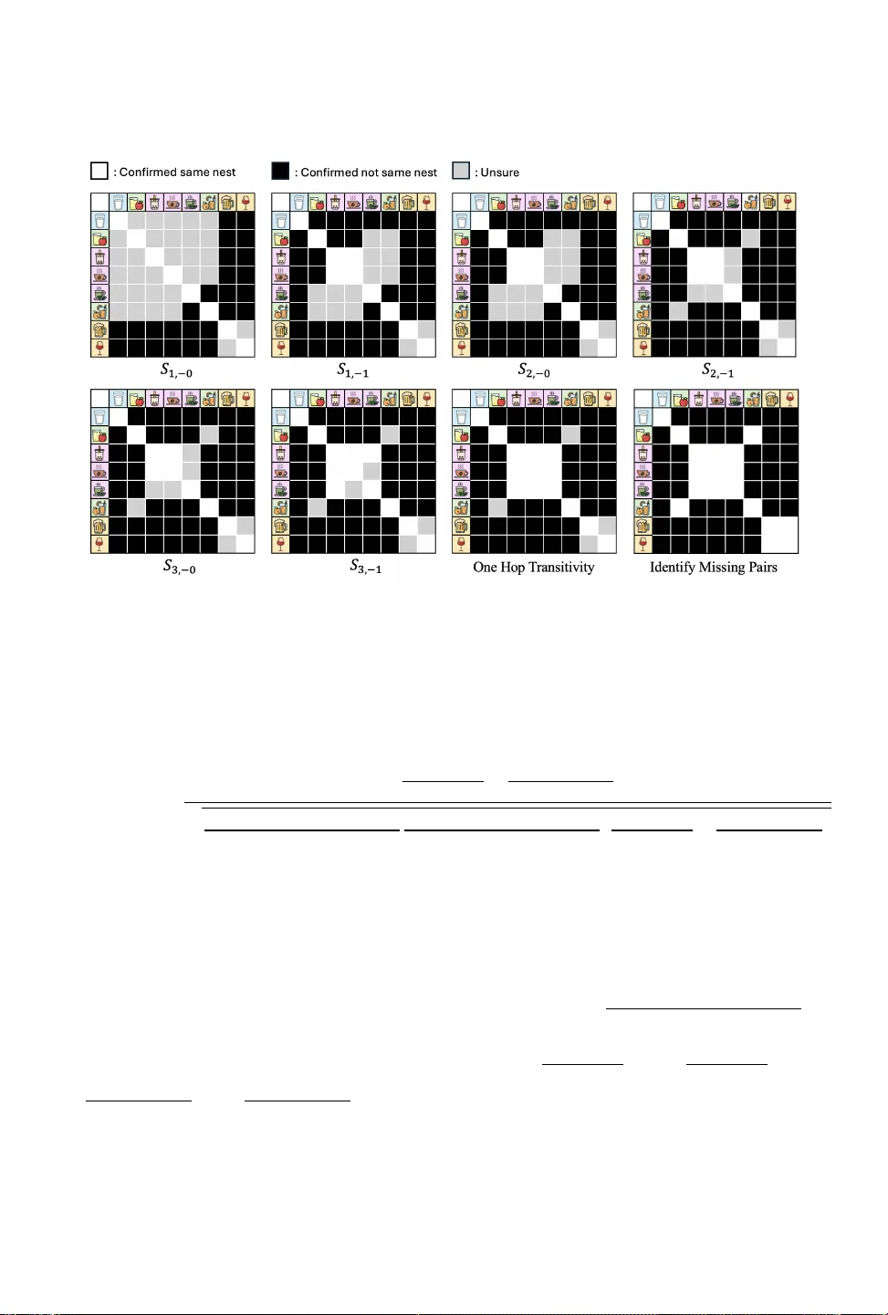
Experimental Assortments for Choice Estimation and Nest Identification XIN TONG YU, Columbia University, XYu29@gsb .columbia.edu WILL MA, Columbia Univ ersity, wm2428@gsb.columbia.edu MICHAEL ZHA O, Dr eam Sports, michael.zhao@dreamsports.group What assortments (subsets of items) should b e oered, to collect data for estimating a choice model over 𝑛 total items? W e propose a structured, non-adaptive experiment design requiring only 𝑂 ( log 𝑛 ) distinct assortments, each oered repeatedly , that consistently outperforms randomized and other heuristic designs across an extensive numerical benchmark that estimates multiple dier ent choice models under a variety of (possibly mis-specie d) ground truths. W e then focus on Nested Logit choice models, which cluster items into "nests" of close substitutes. Whereas existing Nested Logit estimation procedures assume the nests to be known and xed, we present a new algorithm to identify nests based on collected data, which when used in conjunction with our experiment design, guarantees correct identication of nests under any Nested Logit ground truth. Our experiment design was deployed to collect data from ov er 70 million users at Dream11, an Indian fantasy sports platform that oers dierent types of b etting contests, with rich substitution patterns between them. W e identify nests based on the collected data, which lead to b etter out-of-sample choice prediction than ex-ante clustering from contest features. Our identied nests are ex-post justiable to Dream11 management. Contents Abstract 0 Contents 0 1 Introduction 1 2 Related W ork 5 3 Our Experiment Design 8 4 Theoretical Results for Nested Logit 8 5 Numerical Comparison of Experiment Designs 16 6 Numerical Comparison of Nest Identication Algorithms 18 7 Implementation at Dream11 21 8 Concluding Remarks and Future Directions 22 Acknowledgments 23 References 23 A Balanced Experiment Design 25 B Proofs from Section 4 27 C Recovering Remaining Parameters Given the Nest Partition 32 D 𝑑 -level Nested Logit Model 35 E Supplement to Section 5 41 F Supplement to Section 6 42 G Supplement to Section 7 47 Xintong Y u, Will Ma, and Michael Zhao 1 Sales Sales Sales Sales Day 1 200 100 100 100 Day 2 240 120 not oered not oered Day 3 not oered 200 120 120 T able 1. T oy example showing sales of drinks under dier ent assortments oered 1 Introduction Understanding agent choice is important in many applications: a retailer wants to know how customers choose between dierent brands of a product; a car dealer wants to know how buy ers select from its available models; a policymaker wants to know how citizens substitute among transportation modes. The goal is to estimate a choice model, which species for any menu or “assortment” of options, the expected market share that each option would receive. Choice models capture the phenomenon that oering a smaller assortment concentrates mor e market share on each remaining option. In the simplest Multi-Nomial Logit (MNL) choice model, these market shares ar e assumed to all increase by the same %. For example, this is corr oborated by the sales on Day 2 in T able 1: when milk ( ) and boba ( ) were not oered, the sales of apple juice ( ) and orange juice ( ) b oth increased by 20% relative to Day 1, where all drinks were oered. This suggests that on Day 2, some of the customers whose favorite drink would have be en or chose or instead, following a 2 to 1 ratio that is consistent with the sales on Day 1. Howev er , the MNL assumption is often violate d, e.g. on Day 3 in T able 1: when was not oered, the sales of increased disproportionately (doubling r elative to Day 1 sales) compared to the 20% increases of and . This calls for richer choice models such as Nested Logit, which partitions the items into “nests” of close substitutes. Under this model, when a customer’s favorite drink ( ) is not oered, they are more likely to switch to a drink in the same nest (in this case, a dierent juice ) than to drinks in other nests ( , ). Note that fewer total sales were lost on Day 3, because at least one item from each nest was oered, justifying why it may be important to learn the grouping of items into nests. Experiment design problem. Some assortment variation is necessary for learning richer choice models, and this variation may nee d to be deliberately designe d. In the example in T able 1, it is in fact impossible to discern whether and are close substitutes or not, b ecause they were either both oered or both unavailable on each day . This motivates our primary research question. How to deliberately design the assortments oered so that complex substi- tution patterns can be detected and rich choice mo dels can be estimated? This question is largely ignored in papers that estimate empirical choice models, because they use observational data in which the assortments oered were out of the researcher’s control (see Section 2.1). Meanwhile, for papers that estimate choice models fr om synthetic data, they generally draw observations from randomized assortments (see Section 2.2), which do not provide the most ecient form of data collection. In this paper , we introduce a combinatorial design ( explained in Section 1.1) that deliberately arranges the items into a small number of experimental assortments, which are much more infor- mative than randomized assortments. T o demonstrate this, we replicate the numerical framework of Berbeglia et al . [2022], and show that by only replacing their randomized experimental assort- ments while keeping the ground truths and estimation metho ds xed, estimation error is robustly decreased (see Se ction 1.3). That is, even though our experiment design is motivated by Neste d Xintong Y u, Will Ma, and Michael Zhao 2 Logit, it signicantly improves choice model estimation regardless of whether the true and/or estimated models are Nested Logit. For 20 days in Spring 2025, our experiment design was deployed across 70 million users at Dream11 , an Indian fantasy sp orts platform (see Section 1.4). Dream11 oers dierent types of “contests” for users to join, and wants to understand ho w users choose between them. Nest identication problem. After our experiments were deployed, the managers at Dream11 wanted to understand how the contests could be classied into nests of close substitutes. The contests are diverse in many ways, so a priori, it is dicult to subje ctively classify them into nests (the way that one could classify , as “juices”). W e instead want the classication into nests to be based on the data collecte d, which motivates our second research question. How to automatically identify nests based on sales data, instead of relying on subjective classication? Historically , papers on Nested Logit choice estimation ( see Section 2.6) have assumed the nests are xed, focusing instead on estimating the other model parameters for a combination of tractability and interpretability reasons [Train, 2009, §4]. Standard statistics packages (e.g. nlogit in Stata) also make this assumption. Papers that consider nest identication are surprisingly scant, as we discuss in Section 2.6. Our second contribution is to propose a new algorithm for nest identication, based on the simple intuition from T able 1. T o elaborate, for each item in each e xperimental assortment (Day 2, Day 3), we dene its b oost factor to be the ratio of its sales relative to its sales in the control assortment (Day 1) where all items were oered. The algorithm then makes the following two types of deductions. I. ( “Small” Boost Factor ) Because had a “small” b oost factor ( 240 200 = 1 . 2 ) on Day 2, the unavailable items are not close substitutes. That is, neither nor are in the same nest as . W e can similarly deduce that neither nor are in the same nest as . II. ( “Large” Boost Factor ) Because had a “large” boost factor ( 200 100 = 2 ) on Day 3, at least one unavailable item is a close substitute. This item must be , and hence , are in the same nest. Our theoretical algorithm assumes that sales boosts of dierent magnitudes can be p erfectly distinguished, in which case we pr ove that correct nest identication is guaranteed (see Se ction 1.2). W e also de velop an empirical version of the algorithm that handles noise, which we compare to the nest identication algorithm of Benson et al . [2016] on synthetic and real data (see Se ction 1.3). In general, our nest identication algorithm diers from the literature by leveraging repeated observations under a small number of assortments, as motivate d by our experiment design. 1.1 Our Experiment Design Our e xperiment design pr escribes a small number of pre-determined assortments, making it easy to deploy in practical experimentation settings. Indeed, a retail chain may only be able to experiment with one assortment per brick-and-mortar store, and it may want to experiment in parallel, so the outcome of the previous experiment cannot be used to adaptively determine the next assortment. In our drinks example where the randomization is o ver time , each day can only be assigned a single assortment, so our design allows the experimentation to be completed in fewer days. W e now explain our design, for which w e recall the example from T able 1. There, it was possible to deduce that , are in the same nest which does not include or , but not possible to Xintong Y u, Will Ma, and Michael Zhao 3 Oered? ( / ) 000 001 010 011 100 101 110 111 Control Experiment 1 Experiment 2 Experiment 3 Experiment 4 Experiment 5 Experiment 6 T able 2. Our experiment design for 𝑛 = 8 items, requiring 2 ⌈ log 2 𝑛 ⌉ = 6 experimental assortments in addition to the control assortment where all items are oered. The items with their binary encodings are depicted in the columns. deduce whether , are in the same nest. T o rectify this, our experiment design promises the following property: for any ( ordered) pair of items 𝑖 , 𝑗 , there exists an e xperimental assortment 𝑆 containing 𝑖 but not 𝑗 . By looking at the assortment 𝑆 containing but not , we get a sense of how the removal of boosted ’s sales, which helps deduce whether they are in the same nest. T o satisfy this desired property , our experiment design gives each of the 𝑛 items a unique binar y encoding with 𝐿 : = ⌈ log 2 𝑛 ⌉ digits. For each ℓ = 1 , . . . , 𝐿 , we include two experimental assortments: one that contains all items with a “1” in the ℓ ’th digit of their binar y encodings, and the complement assortment that contains all items with a “0” in their ℓ ’th digits. This experiment design satises the desired property , b ecause two distinct items 𝑖 , 𝑗 with unique binary enco dings must have dierent digits for at least one position ℓ , and one of the two experimental assortments 𝑆 for that ℓ will then contain 𝑖 but not 𝑗 . An example of our design for 𝑛 = 8 is given in T able 2. 1.2 Theoretical Results for Nest Identification W e now elaborate on the inferences made by our nest identication algorithm, rst in a noiseless setting where exact market shares under the control and experimental assortments are observed. The goal is to identify a hidden partition N of the items [ 𝑛 ] : = { 1 , . . . , 𝑛 } into nests 𝑁 , satisfying Ð 𝑁 ∈ N 𝑁 = [ 𝑛 ] and 𝑁 ∩ 𝑁 ′ = ∅ for all 𝑁 ≠ 𝑁 ′ . W e make a “general position” assumption that the boost factors of items from dierent nests cannot coincidentally be the same. Under this assumption, we sho w that the following deductions can be made from each experi- mental assortment 𝑆 , which extend the deductions I and II introduced earlier . I. For each nest 𝑁 with 𝑁 ⊆ 𝑆 , we would observe a small boost factor for all items in 𝑁 , which allows us to separate 𝑁 from being in the same nest as any items in [ 𝑛 ] \ 𝑆 . II. For each nest 𝑁 with 𝑁 ⊈ 𝑆 , we would observe a large and distinct b oost factor for all items in 𝑆 ∩ 𝑁 , which allows us to identify that they are all in the same nest, dierent from the nest of any other items in 𝑆 (i.e., we can separate 𝑆 ∩ 𝑁 from 𝑆 \ 𝑁 ). See Figure 1 for an example of these deductions. W e prov e that the hidden partition can be identied using 𝑂 ( log 𝑛 ) non-adaptive assortments, via our experiment design followed by iterating these de ductions over its experimental assortments. That is, given any underlying partition of items into nests, our pipeline is guarante ed to correctly identify the ground truth and hence determine the nests for any Nested Logit choice model. W e also prove that Ω ( log 𝑛 ) queries are necessary , even if adaptiv e. Finally , we consider two extensions. First, relaxing the assumption that exact market shares are observed, we prove nite-sample guarantees for our nest identication algorithms. Second, the preceding deductions assume that an “outside option” (corresponding to not buying anything) can Xintong Y u, Will Ma, and Michael Zhao 4 Fig. 1. Example deductions aer Experiment 1 in T able 2. “Small” boost factors were observed for and , while “large” and distinct b oost factors were observed for and . By deduction I., we know and are not in the same nest as any of the 6 other items, but we do not know whether and are in the same nest. By deduction II., w e know and are also not in the same nest. The table does not record the latent information that both and are in the same nest as at least one item outside 𝑆 , even though this information is necessary for our nest identification. The complete identification of nests is found in Section 4.2.1. always be chosen, and that these choices are observed. W e prove that our experiment design still guarantees correct nest identication without the outside option, by leveraging a more sophisticated nest identication algorithm which operates under weaker forms of deductions I and II. 1.3 Numerical Results Comparing experiment designs. W e compar e our deliberate experiment design to several baselines including randomized assortments, replicating the numerical framework of Berbeglia et al . [2022]. The default setting in Berbeglia et al . [2022] considers a mis-specied ground-truth choice mo del over 10 items. W e show that by changing their random assortments (of sizes 3–6) to our deliberate experiment design, the soft Root Mean Square Error ( RMSE so ) is consistently reduced, under 10 dierent settings from their paper that combine an estimate d choice model (Exponomial, MNL, Latent-class MNL, Nested Logit, or Markov Chain) with a data size. The reduction in RMSE so can be as much as 5.1%, generally being more signicant for small data sizes. The previous comparison assumes that the random design draws the same numb er of experi- mental assortments as our design. If the random design can draw more random assortments, then it can beat our design under large data sizes, while holding the total numb er of observations the same. That being said, if we change to a well-specie d setting wher e both the ground-truth and estimated choice models are Markov Chain, then our experiment design is best across data sizes, even compared to individualized random assortments. The reduction in RMSE so can be as much as 17.2%, under smaller data sizes. Comparing nest identication pip elines. W e compare our nest identication algorithm under our experiment design to the nest identication algorithm of Benson et al . [2016] under their experiment design. Assuming Nested Logit ground truths, our pipeline has massively b etter estimation, reducing the RMSE so by as much as 50%. The main gain comes from experiment design—their pipeline oers assortments of sizes 2 and 3, which provide less information than our assortments of size 𝑛 / 2 . When we test their nest identication algorithm combined with our experiment design, it can actually outperform our nest identication algorithm under small data sizes, because it aggregates observations across assortments, r educing variance. However , this introduces bias, leading to worse performance for large data. Our nest identication algorithm is somewhat attached to our e xperiment design, but we also test it on the publicly-available SF W ork dataset [K oppelman and Bhat, 2006], which has repeated observations but not our deliberate arrangement of assortments. On this dataset, the out-of-sample prediction error of our nest identication algorithm is comparable to that of Benson et al. [2016]. Xintong Y u, Will Ma, and Michael Zhao 5 1.4 Deployment at Dream11 For a span of 20 days in spring 2025, our experiment design was deployed across 70 million users at Dream11. Half of them wer e in the control group and saw all the contest types when deciding which contest to join. For the other 35 million users, w e experimented with 𝑛 = 72 contest typ es. W e created 14 experimental groups based on giving these 72 contests unique 7-digit binar y encodings, ensuring to balance the encodings (see Section A) so that each experimental assortment had ≈ 36 contest types removed. Each e xperimental assortment had to be manually checked by Dream11 management before proceeding, showing that ev en on a digital platform, it can b e important to have a small number of experimental assortments. After collecting the data from our experiment design, we estimate a Nested Logit choice model with nests identied by our algorithm, and show that it consistently beats the simpler MNL mo del on out-of-sample prediction error . Imp ortantly , it also b eats a Nested Logit model with nests determined from 𝑘 -means-clustering on contest features ( e.g., entry fee and contest size), which represents a standard, non-data-driven appr oach to nest identication. Finally , although a Markov Chain choice model beats Nested Logit on prediction error given enough data, an important virtue of our approach is interpr etability: the learned nests reveal meaningful substitution patterns and strike a “sweet spot” between the over-simplied MNL and more exible, higher-parameter alternatives. Roadmap. Our experiment design is presented in Section 3 and tested numerically in Section 5. Our nest identication algorithm is analyzed theoretically in Section 4 and tested numerically in Section 6. Deployment at Dream11 is documented in Section 7. W e pr ovide a concluding discussion in Section 8. 2 Related W ork 2.1 Choice Estimation from Real Data Papers that estimate choice mo dels from real data are often limite d by the quality of the data, like whether product availability information is available in the rst place [Conlon and Mortimer, 2013] and whether lost demand is observed [Vulcano et al . , 2012]. Any further variation in product availability would have to come from stockouts and supply availability [see Bo dea et al . , 2009, Kök and Fisher, 2007], or uctuating covariates such as in a classical D VD dataset [Farias et al . , 2013, Rusmevichientong et al . , 2010]. As a result, these papers are often bound by the data in terms of the choice models they estimate. W e have to our kno wledge a rather unique luxury of estimating choice models from real data, when we also get to control the assortments oered to collect this data. Our focus is therefore on how to design a small number of assortments to “maximize the variation” in product availability , instead of how to handle the lack of information [see Vulcano et al . , 2012] or what is the right choice model complexity given the data at hand [see Farias et al., 2013]. 2.2 Choice Estimation from Randomized Assortments Although synthetic ground truths enable the trial of dierent experiment designs, papers that use them generally default to randomized experimentation. There are examples of dierent randomiza- tion schemes: Chen et al . [2025], Şimşek and T opaloglu [2018] include each item with probability 1/2; Berbeglia et al . [2022], Blanchet et al . [2016] draw random assortments containing between 1/3 to 2/3 of the items; van Ryzin and Vulcano [2015, 2017] draw random assortments with greater variation in sizes. These papers focus on improving the choice estimation procedures, whereas we show that rst-order improvements can be made by combinatorially (instead of randomly ) sele cting the assortments from which data is collected. Xintong Y u, Will Ma, and Michael Zhao 6 2.3 Simple Experiment Designs for Estimation of Specific Choice Models W e mention some non-random experiment designs that have b een used to estimate dierent choice models. For Markov Chain choice models, Blanchet et al . [2016, §2.1] show how to identify all ≈ 𝑛 2 parameters using 𝑛 + 1 assortments, consisting of the grand assortment [ 𝑛 ] and all assortments [ 𝑛 ] \ { 1 } , . . . , [ 𝑛 ] \ { 𝑛 } that remove one item. W e compare to this “Leave-one-out” experiment design in our simulations, which is generally not data-ecient because removing one item has a small eect that is dicult to statistically detect (see Section 5). Meanwhile, for Latent-class MNL choice mo dels, identication is often mor e algebraically in- volved [e .g. Chierichetti et al . , 2018, T ang, 2020]. The identication r esult of Chierichetti et al . [2018] is based on an experiment design that consists of 𝑂 ( 𝑛 ) adaptive or 𝑂 ( 𝑛 2 ) non-adaptive assortments that hav e sizes 2 or 3, which is desirable for solving a system of equations. For Nested Logit, Benson et al . [2016] use an experiment design with 𝑂 ( 𝑛 2 ) adaptively-chosen assortments of sizes 2 or 3 to guarantee identication. For MNL, identication is easy , but Shah et al . [2016] use algebraic metrics to compare experiment designs, focusing on pair wise comparisons, i.e. assortments of size 2. Finally , Chen et al . [2025] consider an e xperiment design for end-to-end assortment optimization in which the rm oers single-item assortments that are w eighed non-uniformly due to asymmetric prices. All in all, opposite to the problem of “Leave-one-out” , the designs from these papers are data-inecient due to being too small and not showing enough items (see Section 6.2). In sum, our e xperiment design has higher general data eciency than all of these designs, thanks to using assortments of size around 𝑛 / 2 , which in some sense 1 maximizes the information per observation. At the same time, it uses fewer assortments than all of them—a sublinear amount 𝑂 ( log 𝑛 ) , based on binar y encodings. T o that end, our theoretical results that guarantee correct identication for Nested Logit (Section 4) are also quite surprising, r elative to results above that require at least linearly many assortments for correct identication. 2.4 Learning while Earning in Assortment Optimization W e also mention a str eam of work on experimental assortments that diers fr om ours by: (i) requiring adaptive experimentation; and (ii) caring about the revenue earned during experimentation. These papers solve a bandit problem over a long horizon, which is ver y dierent in nature than our focus of successful choice estimation after a short horizon (during which not many distinct assortments can be tried). Much work in this stream focuses on the MNL choice model [Agrawal et al . , 2019, Chen et al . , 2021], possibly with covariates [Cheung and Simchi-Levi, 2017, Oh and Iyengar, 2021]. W e defer to the recent paper Li et al. [2025] for further references. 2.5 Combinatorial Design of Experiments Finally , combinatorial arrangements that look similar to ours do frequently appear in the design of experiments, but our assortment setting is quite dierent from the typical setting. T o elaborate, in the typical setting, there is a set of controls (e.g., temperature, time, pressure) that ae ct the outcome of interest, and the goal of the experiment design is to “ cover” dierent interactions between these controls when it is not possible to test all combinations. Common designs in this literature involve orthogonal arrays and Latin squares, dating back to Fisher [1971], T aguchi [1986]. By contrast, in our experiment design, the contr ols are individual items, the outcome is multi-variate (i.e., the item chosen), and the high-level goal is to “separate ” each pair of items. Our deliberate arrangement of assortments ends up being a simple and natural combinatorial design in the conte xt of Colbourn [2010], but to our knowledge, it has not been previously used in experiment design. 1 This intuition is also consistent with the randomized designs discussed in Section 2.2. Xintong Y u, Will Ma, and Michael Zhao 7 2.6 Nested Logit Choice Estimation and Nest Identification Nested Logit has a long history dating back to McFadden [1978], Williams [1977], and is a commonly- used estimation model in both e conometrics [T rain, 2009] and assortment optimization [Gallego and T opaloglu, 2014]. The majority of research on Nested Logit [e.g. Ben-Akiva and Lerman, 1985, Brownstone and Small, 1989, Hensher and Greene, 2002] has focuse d on estimating model parameters (preference w eights for items and dissimilarity parameters for nests) assuming xed nests, noting that ev en this is challenging because the Maximum Likelihood formulation is non- convex. Another e xplanation for nests being xed is that domain knowledge is often strong and desirable to impose (e.g., putting r ed-bus and blue-bus in the same nest; see Train [2009, §4]). That b eing said, several works since have brought to light the issue of nest identication. Benson et al . [2016], Kovach and Tser enjigmid [2022] are similar in spirit, using violations of the Independence of Irrelevant Alternatives (IIA) property between pairs of items 𝑖 , 𝑗 to identify when 𝑖 and 𝑗 should be put into the same nest. Benson et al . [2016] have a more explicit nest identication algorithm that we compare to in Section 6.2, while Ko vach and T serenjigmid [2022, §5] solves a distance minimization pr oblem that has restrictive data r equirements as the number of items grows. Relatedly , Aboutaleb et al . [2020] nd the nest partition and Nested Logit model parameters that collectively maximize likeliho od, formulating the search problem using mixe d- integer programming. Their approach can naturally handle covariates, but also does not scale well in our experiments with more items. These papers also consider multiple levels of nesting, which we discuss in Section D. All in all, our nest identication algorithm diers from these works by anchoring on our ex- periment design, assuming that a small number of experimental assortments S have each be en oered enough times such that the obser ved choice probabilities for each 𝑆 ∈ S (and resulting boost factors) are reliable. Our algorithm does not aggregate observations across assortments, the way that e.g. Benson et al . [2016] considers all assortments containing { 𝑖, 𝑗 } when analyzing IIA for a given pair 𝑖 , 𝑗 , making our algorithm worse on “thin” datasets where each assortment has been observed only once. Regardless, our approach is overall best when experiment design is part of the decision pipeline, as the experiment design suggested by Benson et al . [2016] is data-inecient, oering assortments of a xed small size (2 or 3) in order to stay unbiased (see Se ction F .3), which also causes it to require Ω ( 𝑛 2 ) dierent assortments. 2.7 Graph and Partition Recovery problems Our specic nest identication approach is also related to another stream of work: the oracle query–based graph reconstruction pr oblem. The objective is to recov er a hidden graph by querying oracles that reveal structural information about the graph. A variety of oracle outputs has been studied in the literature. Among them, the ones most closely related to our setting are edge- information oracles [Choi and Kim, 2010, Grebinski and Kucherov, 1998, 2000] and, in more advanced settings, connected-components oracles [Black et al . , 2025, Harviainen and Parviainen, 2025]. Under connected-comp onents oracle, one submits a subset 𝑆 ⊆ 𝑉 and receives either the number of connected components in 𝐺 [ 𝑆 ] [Black et al . , 2025] or the explicit de composition into components [Harviainen and Par viainen, 2025]. Our oracle is tailor ed to Nested Logit and choice modeling, where the underlying graph structure takes the form of cliques, as studied in [Alon and Asodi, 2005]. The oracle returns explicit compo- nents, yet it can provide ev en richer information due to the clique structure of the graph. In prior work, deterministic non-adaptive bounds range from Ω ( 𝑛 log 𝑛 ) to 𝑂 ( 𝑛 log 2 𝑛 ) for edge-existence queries on vertex subsets [Alon and Asodi, 2005], while randomized adaptive methods achieve Xintong Y u, Will Ma, and Michael Zhao 8 𝑂 ( 𝑛 log 𝑛 ) for general graph reconstruction [Harviainen and Parviainen, 2025]. By contrast, lever- aging both the oracle output and the clique structure reduces the complexity to 𝑂 ( log 𝑛 ) in the deterministic non-adaptive setting. 2.8 Substitute Detection via Price V ariation A classical goal in empirical demand analysis is to recover own- and cross-price elasticities (or related substitution objects) from a demand system [ e.g. Deaton and Muellbauer, 1980], with structural discrete-choice models often used to infer substitution patterns while addr essing endogeneity of prices/attributes using instruments [Berry et al . , 1995, Nevo, 2000]. These inuential frameworks focus on identication from obser vational price variation and endogeneity , whereas our setting assumes the ability to randomly experiment with product availability , where remo ving a product from the assortment is like setting its price to ∞ . A closer conceptual comparison is Li et al . [2015], who ask how many price experiments are needed to learn a cross-elasticity matrix. They have a similar punchline that 𝑂 ( log 𝑛 ) experiments suce, but through very dierent mechanisms—in fact, randomized experiments work in their setting, but only under structural assumptions on the sparsity of the elasticity matrix, which depend on the continuous nature of pricing. By contrast, our 𝑂 ( log 𝑛 ) result comes from our deliberate experiment design that “separates” pairs of items, and also our discrete combinatorial reasoning about nests (see Theorems 4.5 and 4.8). 3 Our Experiment Design Let there be 𝑛 items, denoted by the set [ 𝑛 ] where [ 𝑛 ] : = { 1 , . . . , 𝑛 } . Our experiment design gives each item 𝑖 ∈ [ 𝑛 ] an encoding in base 𝑏 ≥ 2 (the Introduction only considered 𝑏 = 2 and binar y encodings). W e consider enco dings with 𝐿 = ⌈ log 𝑏 𝑛 ⌉ digits, which ensur es that each item can have a unique encoding be cause 𝑏 𝐿 ≥ 𝑛 . W e let 𝜎 ( 𝑖 ) denote the base- 𝑏 encoding given to item 𝑖 , with 𝜎 ℓ ( 𝑖 ) ∈ { 0 , . . . , 𝑏 − 1 } denoting the digit in position ℓ for all ℓ = 1 , . . . , 𝐿 . W e place no requirements on the encodings other than two distinct items cannot have the same encoding. Given these encodings, our experiment design S consists of the following 𝑏 𝐿 assortments: 𝑆 ℓ , − 𝑑 : = { 𝑖 ∈ [ 𝑛 ] : 𝜎 ℓ ( 𝑖 ) ≠ 𝑑 } ∀ ℓ = 1 , . . . , 𝐿 ; 𝑑 = 0 , . . . , 𝑏 − 1 . W e assume that the control assortment [ 𝑛 ] is also oered, in addition to the assortments in S . T able 2 illustrates our design for 𝑛 = 8 and 𝑏 = 2 , with the experimental assortments appearing in order 𝑆 1 , − 0 , 𝑆 1 , − 1 , 𝑆 2 , − 0 , 𝑆 2 , − 1 , 𝑆 3 , − 0 , 𝑆 3 , − 1 . A simple encoding 𝜎 would b e to map each item 𝑖 ∈ [ 𝑛 ] to the number 𝑖 − 1 in base 𝑏 . Howev er , we also provide in Section A a more “balanced” encoding algorithm wher e all experimental assortments have a similar size, i.e . max ℓ , 𝑑 | 𝑆 ℓ , − 𝑑 | − min ℓ , 𝑑 | 𝑆 ℓ , − 𝑑 | ≤ 1 . 4 Theoretical Results for Nested Logit For all assortments 𝑆 ⊆ [ 𝑛 ] , a choice function 𝜙 ( 𝑖 , 𝑆 ) species the probability that each item 𝑖 ∈ 𝑆 would be chosen when assortment 𝑆 is oered. By default, we assume the existence of an outside option 𝑖 = 0 that could also be chosen, in which case the choice probabilities satisfy Í 𝑖 ∈ 𝑆 ∪ { 0 } 𝜙 ( 𝑖 , 𝑆 ) = 1 . (W e consider the case without outside option in Section 4.4.) Our theoretical results assume a specic parametric form for the choice function 𝜙 , namely that it is dened by Neste d Logit 2 . That is, there is a partition N consisting of nests 𝑁 ⊆ [ 𝑛 ] , satisfying Ø 𝑁 ∈ N 𝑁 = [ 𝑛 ] , 𝑁 ∩ 𝑁 ′ = ∅ ∀ 𝑁 ≠ 𝑁 ′ . 2 W e also describe a generalized 𝑑 -level Nested Logit model in Section D. Xintong Y u, Will Ma, and Michael Zhao 9 Each item 𝑖 is associated with a prefer ence weight 𝑣 𝑖 > 0 , and each nest 𝑁 ∈ N is associated with a dissimilarity parameter 𝜆 𝑁 ∈ [ 0 , 1 ] , where a smaller 𝜆 𝑁 indicates greater within-nest correlation for nest 𝑁 . 𝜆 𝑁 ∈ [ 0 , 1 ] is customary for ensuring a choice model consistent with random utility maximization, where w e defer to Gallego and T opaloglu [2014] for more background on Nested Logit. The preference weight for a nest 𝑁 within a subset 𝑆 ⊆ [ 𝑛 ] is dened as: 𝑣 𝑁 ( 𝑆 ) : = ( ( Í 𝑖 ∈ 𝑁 ∩ 𝑆 𝑣 𝑖 ) 𝜆 𝑁 𝜆 𝑁 ∈ ( 0 , 1 ] 𝑣 𝑁 1 ( 𝑁 ∩ 𝑆 ≠ ∅ ) 𝜆 𝑁 = 0 noting that if 𝜆 𝑁 = 0 , then nest 𝑁 has an extra parameter 𝑣 𝑁 for the preference weight of the nest. Let 𝑁 ( 𝑖 ) denote the nest to which item 𝑖 belongs. W e note the special case 𝜆 𝑁 = 0 . When oered an assortment 𝑆 ⊆ [ 𝑛 ] , the probability of 𝑖 ∈ 𝑆 being chosen is: 𝜙 ( 𝑖 , 𝑆 ) = 𝑃 ( 𝑁 ( 𝑖 ) | 𝑆 ) · 𝑃 ( 𝑖 | 𝑁 ( 𝑖 ) , 𝑆 ) where (1) 𝑃 ( 𝑁 ( 𝑖 ) | 𝑆 ) = 𝑣 𝑁 ( 𝑖 ) ( 𝑆 ) 1 + Í 𝑁 ∈ N 𝑣 𝑁 ( 𝑆 ) and 𝑃 ( 𝑖 | 𝑁 ( 𝑖 ) , 𝑆 ) = 𝑣 𝑖 Í 𝑗 ∈ 𝑁 ( 𝑖 ) ∩ 𝑆 𝑣 𝑗 . (2) Here in the Nested Logit model, 𝑃 ( 𝑁 ( 𝑖 ) | 𝑆 ) denotes the probability of nest 𝑁 ( 𝑖 ) rst being chosen from 𝑆 , and 𝑃 ( 𝑖 | 𝑁 ( 𝑖 ) , 𝑆 ) denotes the probability of 𝑖 being chosen conditional on 𝑁 ( 𝑖 ) being chosen from 𝑆 . The “1” in the denominator corresponds to the outside option, which has a weight normalized to 1 and is always in its own nest. The probability of the outside option b eing chosen is 𝜙 ( 0 , 𝑆 ) = 1 1 + Í 𝑁 ∈ N 𝑣 𝑁 ( 𝑆 ) , noting that this ensures Í 𝑖 ∈ 𝑆 ∪ { 0 } 𝜙 ( 𝑖 , 𝑆 ) = 1 . Assumption 1 (Identifiability). 𝜆 𝑁 = 1 if and only if | 𝑁 | = 1 . Assumption 1 prev ents identiability issues in which dierent nest partitions induce the same choice probabilities 𝜙 ( 𝑖 , 𝑆 ) , and can be made without loss of generality . Indeed, any nest 𝑁 with 𝜆 𝑁 = 1 and | 𝑁 | > 1 can be replaced by | 𝑁 | singleton nests without aecting the choice probabilities. Conversely , a singleton nest 𝑁 = { 𝑖 } with 𝜆 𝑁 < 1 can be reparameterized as a nest whose item 𝑖 has new weight 𝑣 𝜆 𝑁 𝑖 (or 𝑣 𝑁 if 𝜆 𝑁 = 0 ) and then 𝜆 𝑁 is changed to 1. Denition 4.1 (Nest Identication Problem, noiseless version). Given a set of experimental assort- ments S under a Nested Logit model, we observe choice probabilities 𝜙 ( 𝑖 , 𝑆 ) for all 𝑖 ∈ 𝑆 ∪ { 0 } and 𝑆 ∈ S ∪ { [ 𝑛 ] } . The goal is to recover the underlying nest partition N . 4.1 Boost Factors and De ductions about Nest Membership The key idea is to examine the boost in an item’s choice probability in an experimental assortment 𝑆 ∈ S , compared to the control assortment [ 𝑛 ] where all items are oered. Denition 4.2 (Boost Factors). For all 𝑆 ∈ S , dene the bo ost factor seen by item 𝑖 ∈ 𝑆 ∪ { 0 } as BF ( 𝑖 , 𝑆 ) : = 𝜙 ( 𝑖 , 𝑆 ) 𝜙 ( 𝑖 , [ 𝑛 ] ) . Xintong Y u, Will Ma, and Michael Zhao 10 Using Equation (2) for the Nested Logit model, we obtain the following: BF ( 𝑖 , 𝑆 ) = 𝑣 𝑁 ( 𝑖 ) ( 𝑆 ) 1 + Í 𝑁 ∈ N 𝑣 𝑁 ( 𝑆 ) · 𝑣 𝑖 Í 𝑗 ∈ 𝑁 ( 𝑖 ) ∩ 𝑆 𝑣 𝑗 𝑣 𝑁 ( 𝑖 ) ( [ 𝑛 ] ) 1 + Í 𝑁 ∈ N 𝑣 𝑁 ( [ 𝑛 ] ) · 𝑣 𝑖 Í 𝑗 ∈ 𝑁 ( 𝑖 ) 𝑣 𝑗 = Í 𝑗 ∈ 𝑁 ( 𝑖 ) 𝑣 𝑗 Í 𝑗 ∈ 𝑁 ( 𝑖 ) ∩ 𝑆 𝑣 𝑗 1 − 𝜆 𝑁 ( 𝑖 ) · 1 + Í 𝑁 ∈ N 𝑣 𝑁 ( [ 𝑛 ] ) 1 + Í 𝑁 ∈ N 𝑣 𝑁 ( 𝑆 ) ∀ 𝑖 ∈ 𝑆 , BF ( 0 , 𝑆 ) = 𝜙 ( 0 , 𝑆 ) 𝜙 ( 0 , [ 𝑛 ] ) = 1 + Í 𝑁 ∈ N 𝑣 𝑁 ( [ 𝑛 ] ) 1 + Í 𝑁 ∈ N 𝑣 𝑁 ( 𝑆 ) , noting that formula for BF ( 𝑖 , 𝑆 ) is correct even if 𝜆 𝑁 ( 𝑖 ) = 0 . Thus, we have BF ( 𝑖 , 𝑆 ) = Mult ( 𝑁 ( 𝑖 ) , 𝑆 ) BF ( 0 , 𝑆 ) , where Mult ( 𝑁 , 𝑆 ) : = Í 𝑗 ∈ 𝑁 𝑣 𝑗 Í 𝑗 ∈ 𝑁 ∩ 𝑆 𝑣 𝑗 1 − 𝜆 𝑁 is a nest-dependent multiplier that, importantly , does not de- pend on the spe cic item. For a nest 𝑁 ∈ N such that 𝑁 ∩ 𝑆 ≠ ∅ , we note the following about Mult ( 𝑁 , 𝑆 ) : I. If 𝑁 ⊆ 𝑆 , then Mult ( 𝑁 , 𝑆 ) = 1 , and hence BF ( 𝑖 , 𝑆 ) = BF ( 0 , 𝑆 ) for all 𝑖 ∈ 𝑁 ∩ 𝑆 ; II. If 𝑁 ⊈ 𝑆 , then | 𝑁 | ≥ 2 , since 𝑁 ∩ 𝑆 ≠ ∅ . Under Assumption 1, this means that 𝜆 𝑁 < 1 , and hence Mult ( 𝑁 , 𝑆 ) > 1 , with BF ( 𝑖 , 𝑆 ) = BF ( 𝑗 , 𝑆 ) > BF ( 0 , 𝑆 ) for all 𝑖 , 𝑗 ∈ 𝑁 ∩ 𝑆 . W e now make a “general p osition” assumption that for two dierent nests not contained in 𝑆 , their multipliers (which are strictly gr eater than 1) cannot coincidentally be the same. Assumption 2 (General P osition). For all 𝑆 ∈ S and two dierent nests 𝑁 ≠ 𝑁 ′ such that ∅ ≠ 𝑁 ∩ 𝑆 ≠ 𝑁 and ∅ ≠ 𝑁 ′ ∩ 𝑆 ≠ 𝑁 ′ , we have Mult ( 𝑁 , 𝑆 ) ≠ Mult ( 𝑁 ′ , 𝑆 ) . T wo items 𝑖 , 𝑗 in the same nest are guaranteed to see the same bo ost factor , regardless of whether this boost factor equals BF ( 0 , 𝑆 ) . Assumption 2 ensures the converse , where if 𝑁 ( 𝑖 ) ≠ 𝑁 ( 𝑗 ) , then it must be that BF ( 𝑖 , 𝑆 ) ≠ BF ( 𝑗 , 𝑆 ) , except in the case wher e both 𝑁 ( 𝑖 ) ⊆ 𝑆 , 𝑁 ( 𝑗 ) ⊆ 𝑆 and we see BF ( 𝑖 , 𝑆 ) = BF ( 𝑗 , 𝑆 ) = BF ( 0 , 𝑆 ) . Example 4.3. Continuing the example from T able 2, consider Experiment 2, which oers the assort- ment 𝑆 : = 𝑆 1 , − 1 = { , , , } . Suppose we see the bo ost factors BF ( , 𝑆 ) = 1 . 3 , BF ( , 𝑆 ) = 1 . 6 , BF ( , 𝑆 ) = 1 . 9 , BF ( , 𝑆 ) = 1 . 9 , and BF ( 0 , 𝑆 ) = 1 . 3 . W e can take the contrapositives of the preced- ing observations to make the following deductions about nest memb ership. • 𝑁 ( ) ⊆ 𝑆 , because if 𝑁 ( ) ⊈ 𝑆 then we would hav e seen BF ( , 𝑆 ) > BF ( 0 , 𝑆 ) , which is not the case. From this w e can deduce that 𝑁 ( ) ≠ 𝑁 ( 𝑘 ) for all 𝑘 ∉ 𝑆 . • 𝑁 ( ) = 𝑁 ( ) , because if 𝑁 ( ) ≠ 𝑁 ( ) then we cannot coincidentally see BF ( , 𝑆 ) = BF ( , 𝑆 ) , by Assumption 2. • { } , { } , and { , } are all part of dierent nests. This is simply taking the contrapositive of the fact that items in the same nest see the same boost factor under each assortment 𝑆 . W e now summarize the observations from this section in the following Proposition. Proposition 4.4 (Nest Deductions with Outside Option). Supp ose Assumption 1 and 2 hold and take any 𝑆 ∈ S . For all 𝑖 ∈ 𝑆 : I. If 𝑁 ( 𝑖 ) ⊆ 𝑆 , then we see that BF ( 𝑖 , 𝑆 ) = BF ( 0 , 𝑆 ) ; II. If 𝑁 ( 𝑖 ) ⊈ 𝑆 , then we se e that BF ( 𝑖 , 𝑆 ) > BF ( 0 , 𝑆 ) , and moreover for 𝑗 ∈ 𝑆 \ { 𝑖 } , we have 𝑁 ( 𝑖 ) = 𝑁 ( 𝑗 ) if and only if BF ( 𝑖 , 𝑆 ) = BF ( 𝑗 , 𝑆 ) . Therefore , we can make the following deductions about nest membership. • If 𝑖 ∈ 𝑆 and BF ( 𝑖 , 𝑆 ) = BF ( 0 , 𝑆 ) , then 𝑁 ( 𝑖 ) ≠ 𝑁 ( 𝑘 ) for all 𝑘 ∉ 𝑆 . • If 𝑖 , 𝑗 ∈ 𝑆 and BF ( 𝑖 , 𝑆 ) = BF ( 𝑗 , 𝑆 ) > BF ( 0 , 𝑆 ) , then 𝑁 ( 𝑖 ) = 𝑁 ( 𝑗 ) . • If 𝑖 , 𝑗 ∈ 𝑆 and BF ( 𝑖 , 𝑆 ) ≠ BF ( 𝑗 , 𝑆 ) , then 𝑁 ( 𝑖 ) ≠ 𝑁 ( 𝑗 ) . Xintong Y u, Will Ma, and Michael Zhao 11 4.2 Nest Identification Algorithm and Proof of Correctness Our algorithms employ a graph-the oretic r epresentation for the nest identication proce dure . Each item corresponds to a vertex, and an edge exists between vertices 𝑖 and 𝑗 whenever 𝑁 ( 𝑖 ) = 𝑁 ( 𝑗 ) . The pairwise relations are recorded in a matrix 𝐸 ∈ { 0 , 1 , null } 𝑛 × 𝑛 . Here, 𝐸 [ 𝑖 , 𝑗 ] = 1 indicates that 𝑁 ( 𝑖 ) = 𝑁 ( 𝑗 ) ; 𝐸 [ 𝑖 , 𝑗 ] = 0 indicates that 𝑁 ( 𝑖 ) ≠ 𝑁 ( 𝑗 ) ; and 𝐸 [ 𝑖 , 𝑗 ] = null indicates that their relation is currently undetermined. The identication task is complete once 𝐸 represents a collection of disjoint cliques, each corresponding to a distinct nest. Our nest identication algorithm is presented in Algorithm 1. W e note that the symmetr y of matrix 𝐸 is preserved throughout the algorithm, and we ignore the values of 𝐸 along the diagonal, where we implicitly assume 𝑖 ≠ 𝑗 whenever we consider pairs 𝑖 , 𝑗 in Algorithm 1. Algorithm 1 Exact Nest Identifica tion with Outside Option 1: Initialize adjacency matrix 𝐸 [ 𝑖, 𝑗 ] ← null for all 𝑖 , 𝑗 ∈ [ 𝑛 ] 2: for 𝑆 ∈ S do 3: for 𝑖 , 𝑗 ∈ 𝑆 do 4: if BF ( 𝑖 , 𝑆 ) ≠ BF ( 𝑗 , 𝑆 ) then 5: 𝐸 [ 𝑖 , 𝑗 ] ← 0 6: else if BF ( 𝑖 , 𝑆 ) = BF ( 𝑗 , 𝑆 ) > BF ( 0 , 𝑆 ) then 7: 𝐸 [ 𝑖 , 𝑗 ] ← 1 8: end if 9: end for 10: NoBoost ← { 𝑖 ∈ 𝑆 : BF ( 𝑖 , 𝑆 ) = BF ( 0 , 𝑆 ) } 11: 𝐸 [ 𝑖, 𝑘 ] ← 0 and 𝐸 [ 𝑘 , 𝑖 ] ← 0 for all 𝑖 ∈ NoBoost and all 𝑘 ∉ 𝑆 12: end for 13: OneHop Transitivity ← { ( 𝑖 , 𝑗 ) ∈ [ 𝑛 ] 2 : 𝐸 [ 𝑖 , 𝑗 ] = null , ∃ 𝑘 ∉ { 𝑖 , 𝑗 } s.t. 𝐸 [ 𝑖 , 𝑘 ] = 𝐸 [ 𝑗 , 𝑘 ] = 1 } 14: 𝐸 [ 𝑖, 𝑗 ] ← 1 for all ( 𝑖 , 𝑗 ) ∈ OneHop Transitivity 15: IdentifyMissingPairs ← { ( 𝑖 , 𝑗 ) ∈ [ 𝑛 ] 2 : 𝐸 [ 𝑖 , 𝑗 ] = null , 𝐸 [ 𝑖 , 𝑘 ] ≠ 1 ≠ 𝐸 [ 𝑗 , 𝑘 ] ∀ 𝑘 ∉ { 𝑖, 𝑗 } } 16: 𝐸 [ 𝑖, 𝑗 ] ← 1 for all ( 𝑖 , 𝑗 ) ∈ IdentifyMissingPairs 17: 𝐸 [ 𝑖 , 𝑗 ] ← 0 for all 𝑖 , 𝑗 ∈ [ 𝑛 ] such that 𝐸 [ 𝑖, 𝑗 ] = null Theorem 4.5 (proven in Section B.1). Suppose that true market shares 𝜙 ( 𝑖 , 𝑆 ) are observed for all 𝑆 ∈ S ∪ { [ 𝑛 ] } and 𝑖 ∈ 𝑆 ∪ { 0 } . Under Assumptions 1 and 2, the adjacency matrix 𝐸 returned by Algorithm 1 satises 𝐸 [ 𝑖 , 𝑗 ] = 1 ( 𝑁 ( 𝑖 ) = 𝑁 ( 𝑗 ) ) for all 𝑖 ≠ 𝑗 , i.e., Algorithm 1 is correct. The correctness of the deductions on lines 5, 7, and 11 of Algorithm 1 follow fr om Proposition 4.4. The proof of Theorem 4.5 is about showing that all nests are ev entually found, i.e. the matrix 𝐸 is completed, which requires the “One Hop Transitivity” and “Identify Missing Pairs” operations. Tightness. Algorithm 1 and Theorem 4.5 show that our non-adaptive experimental design with 𝑂 ( log 𝑛 ) assortments is sucient to guarantee nest identication. W e prove in Section B.2 that Ω ( log 𝑛 ) experimental assortments are also necessar y , even if adaptively selected. Extensions and loose ends. W e show in Section C that, under a mild non-degeneracy condition (A ssumption 3), our experiment design also allows successful recovery of the Nested Logit parame- ters ( 𝑣 𝑖 ) 𝑖 ∈ [ 𝑛 ] , ( 𝜆 𝑁 ) 𝑁 ∈ N , and 𝑣 𝑁 for nests 𝑁 with 𝜆 𝑁 = 0 , after identifying the nests. W e discuss the 𝑑 -level Nested Logit model in Section D. 4.2.1 Illustration of Algorithm 1. T o illustrate the logical deductions made by our nest identi- cation algorithm, we r eturn to the example from Table 2. W e provide hypothetical results for all experimental assortments in T able 3, where we split the items in each experiment 𝑆 ∈ S into equivalence classes based on their observed b oost factors, further indicating the class that equals Xintong Y u, Will Ma, and Michael Zhao 12 Item and Encoding 000 001 010 011 100 101 110 111 Boost Factors in 𝑆 1 , − 0 ↑ ( 1 ) ↑ ( 2 ) – – Boost Factors in 𝑆 1 , − 1 – ↑ ( 1 ) ↑ ( 2 ) ↑ ( 2 ) Boost Factors in 𝑆 2 , − 0 ↑ ( 1 ) ↑ ( 1 ) – – Boost Factors in 𝑆 2 , − 1 – – ↑ ( 1 ) – Boost Factors in 𝑆 3 , − 0 – ↑ ( 1 ) – ↑ ( 2 ) Boost Factors in 𝑆 3 , − 1 – ↑ ( 1 ) ↑ ( 1 ) ↑ ( 2 ) T able 3. Hypothetical results for the e xperiment design from T able 2. “ – ” indicates a boost factor equal to BF ( 0 , 𝑆 ) . Items indicated by “ ↑ ( 1 ) ” share the same b oost factor greater than BF ( 0 , 𝑆 ) ; items indicated by “ ↑ ( 2 ) ” share a dierent boost factor greater than BF ( 0 , 𝑆 ) , etc. BF ( 0 , 𝑆 ) . Our algorithm is purely combinatorial and does not use the exact numerical magnitudes of boost factors. Figure 2 then shows the evolution of the 𝐸 [ 𝑖 , 𝑗 ] matrix throughout the steps of Algorithm 1. The rst 6 steps make deductions from the 6 experimental assortments, and the nal two steps demonstrate the importance of the “One Hop T ransitivity” and “Identify Missing Pairs” operations. The deductions from the 1st assortment were previously illustrate d in Figur e 1, while the deductions from 2nd assortment were pr eviously illustrated in Example 4.3. 4.3 Finite-sample Guarantee Recall that our nest identication Algorithm 1 is based on comparing boost factors, BF ( 𝑖 , 𝑆 ) = 𝜙 ( 𝑖 , 𝑆 ) / 𝜙 ( 𝑖 , [ 𝑛 ] ) , across 𝑖 ∈ 𝑆 ∪ { 0 } for each experimental assortment 𝑆 ∈ S . W e now discuss how to do nest identication if the choice probabilities 𝜙 ( 𝑖 , 𝑆 ) are observed only approximately . In particular , we assume that we obser ve 𝑚 independently sampled choices from each assortment 𝑆 ∈ S ∪ { [ 𝑛 ] } , and let ˆ 𝜙 ( 𝑖 , 𝑆 ) denote the empirical probability that each 𝑖 ∈ 𝑆 ∪ { 0 } is chosen from 𝑆 over these 𝑚 samples. W e deriv e a bound on 𝑚 that allows for the nest partition N to be corr ectly identied with high probability . A naiv e approach would be to compare “ empirical” boost factors, ˆ 𝜙 ( 𝑖 ,𝑆 ) ˆ 𝜙 ( 𝑖 , [ 𝑛 ] ) , but that is a biased esti- mator . W e instead rewrite the comparison BF ( 𝑖 , 𝑆 ) ≥ BF ( 𝑗 , 𝑆 ) as a comparison of two probabilities, allowing us to appeal to standard statistical tests. In particular , BF ( 𝑖 , 𝑆 ) ≥ BF ( 𝑗 , 𝑆 ) ⇐ ⇒ 𝜙 ( 𝑖 , 𝑆 ) 𝜙 ( 𝑖 , [ 𝑛 ] ) ≥ 𝜙 ( 𝑗 , 𝑆 ) 𝜙 ( 𝑗 , [ 𝑛 ] ) ⇐ ⇒ 𝜙 ( 𝑖 , 𝑆 ) 𝜙 ( 𝑗 , 𝑆 ) ≥ 𝜙 ( 𝑖 , [ 𝑛 ] ) 𝜙 ( 𝑗 , [ 𝑛 ] ) ⇐ ⇒ 𝜙 ( 𝑖 , 𝑆 ) 𝜙 ( 𝑖 , 𝑆 ) + 𝜙 ( 𝑗 , 𝑆 ) ≥ 𝜙 ( 𝑖 , [ 𝑛 ] ) 𝜙 ( 𝑖 , [ 𝑛 ] ) + 𝜙 ( 𝑗 , [ 𝑛 ] ) ∀ 𝑆 ∈ S ; 𝑖 , 𝑗 ∈ 𝑆 ∪ { 0 } . (3) The LHS and RHS of (3) can b e interpreted as the “probability of choosing 𝑖 conditional on choosing 𝑖 or 𝑗 ” in assortments 𝑆 and [ 𝑛 ] , respectively . Xintong Y u, Will Ma, and Michael Zhao 13 Fig. 2. Evolution of the adjacency matrix 𝐸 during nest identification. White squares indicate 𝐸 [ 𝑖, 𝑗 ] = 1 (same nest); black squares indicate 𝐸 [ 𝑖, 𝑗 ] = 0 (dier ent nests); while gre y squares indicate 𝐸 [ 𝑖, 𝑗 ] = null (not yet determined). The state of the adjacency matrix 𝐸 is displayed aer processing each of the 6 experimental assortments 𝑆 ∈ S , and aer the “One Hop Transitivity” (line (14) ) and “Identify Missing Pairs” (line (16) ) operations. The pooled two-proportion test statistic is then dened as 𝑧 ( 𝑖 ≻ 𝑗 , 𝑆 ) : = ˆ 𝜙 ( 𝑖 ,𝑆 ) ˆ 𝜙 ( 𝑖 ,𝑆 ) + ˆ 𝜙 ( 𝑗 ,𝑆 ) − ˆ 𝜙 ( 𝑖 , [ 𝑛 ] ) ˆ 𝜙 ( 𝑖 , [ 𝑛 ] ) + ˆ 𝜙 ( 𝑗 , [ 𝑛 ] ) ˆ 𝜙 ( 𝑖 ,𝑆 ) + ˆ 𝜙 ( 𝑖 , [ 𝑛 ] ) ˆ 𝜙 ( 𝑖 ,𝑆 ) + ˆ 𝜙 ( 𝑗 ,𝑆 ) + ˆ 𝜙 ( 𝑖 , [ 𝑛 ] ) + ˆ 𝜙 ( 𝑗 , [ 𝑛 ] ) ˆ 𝜙 ( 𝑗 ,𝑆 ) + ˆ 𝜙 ( 𝑗 , [ 𝑛 ] ) ˆ 𝜙 ( 𝑖 ,𝑆 ) + ˆ 𝜙 ( 𝑗 ,𝑆 ) + ˆ 𝜙 ( 𝑖 , [ 𝑛 ] ) + ˆ 𝜙 ( 𝑗 , [ 𝑛 ] ) ( 1 / 𝑚 ˆ 𝜙 ( 𝑖 ,𝑆 ) + ˆ 𝜙 ( 𝑗 ,𝑆 ) + 1 / 𝑚 ˆ 𝜙 ( 𝑖 , [ 𝑛 ] ) + ˆ 𝜙 ( 𝑗 , [ 𝑛 ] ) ) , (4) where highly positive values suggest BF ( 𝑖 , 𝑆 ) > BF ( 𝑗 , 𝑆 ) , highly negative values suggest BF ( 𝑖 , 𝑆 ) < BF ( 𝑗 , 𝑆 ) , and otherwise BF ( 𝑖 , 𝑆 ) = BF ( 𝑗 , 𝑆 ) is accepte d as the default or “null” hypothesis. The intuition behind the formula for 𝑧 ( 𝑖 ≻ 𝑗 , 𝑆 ) is that dierences in the numerator are amplied (i.e., we ar e more condent in directional dierences in the numerator probabilities) if 𝑚 is large (higher condence with more samples), if ˆ 𝜙 ( 𝑖 , 𝑆 ) + ˆ 𝜙 ( 𝑗 , 𝑆 ) and ˆ 𝜙 ( 𝑖 , [ 𝑛 ] ) + ˆ 𝜙 ( 𝑗 , [ 𝑛 ] ) are both large ( higher con- dence if many comparisons between 𝑖 and 𝑗 ), or if the “po oled” mean ˆ 𝜙 ( 𝑖 ,𝑆 ) + ˆ 𝜙 ( 𝑖 , [ 𝑛 ] ) ˆ 𝜙 ( 𝑖 ,𝑆 ) + ˆ 𝜙 ( 𝑗 ,𝑆 ) + ˆ 𝜙 ( 𝑖 , [ 𝑛 ] ) + ˆ 𝜙 ( 𝑗 , [ 𝑛 ] ) is close to 0 or 1 (higher condence if the probability is more deterministic). W e note that 𝑧 ( 𝑖 ≻ 𝑗 , 𝑆 ) = − 𝑧 ( 𝑗 ≻ 𝑖 , 𝑆 ) , because the numerator satises ˆ 𝜙 ( 𝑖 ,𝑆 ) ˆ 𝜙 ( 𝑖 ,𝑆 ) + ˆ 𝜙 ( 𝑗 ,𝑆 ) = 1 − ˆ 𝜙 ( 𝑗 ,𝑆 ) ˆ 𝜙 ( 𝑖 ,𝑆 ) + ˆ 𝜙 ( 𝑗 ,𝑆 ) and ˆ 𝜙 ( 𝑖 , [ 𝑛 ] ) ˆ 𝜙 ( 𝑖 , [ 𝑛 ] ) + ˆ 𝜙 ( 𝑗 , [ 𝑛 ] ) = 1 − ˆ 𝜙 ( 𝑗 , [ 𝑛 ] ) ˆ 𝜙 ( 𝑖 , [ 𝑛 ] ) + ˆ 𝜙 ( 𝑗 , [ 𝑛 ] ) while the denominator is symmetric in 𝑖 and 𝑗 . Statistically speaking, 𝑧 ( 𝑖 ≻ 𝑗 , 𝑆 ) is asymptotically Normal with mean 0 and standard de viation 1, whose CDF we denote using Φ . W e can compare 𝑧 ( 𝑖 ≻ 𝑗 , 𝑆 ) to absolute constants such as Φ − 1 ( 0 . 025 ) ≈ − 2 or Φ − 1 ( 0 . 975 ) ≈ 2 , and e.g. reject the null hyp othesis that BF ( 𝑖 , 𝑆 ) = BF ( 𝑗 , 𝑆 ) if 𝑧 ( 𝑖 ≻ 𝑗 , 𝑆 ) ∉ [ − 2 , 2 ] . W e will use such comparisons when we test our nest identication algorithms Xintong Y u, Will Ma, and Michael Zhao 14 empirically in Section 6; for our the oretical result below , we compare 𝑧 ( 𝑖 ≻ 𝑗 , 𝑆 ) to a constant that depends on the number of items 𝑛 and the tolerable failure probability 𝛿 . Theorem 4.6 (proven in Section B.3). T ake constants 𝜌 , Δ , 𝛿 ∈ ( 0 , 1 ) such that 𝜙 ( 𝑖 , [ 𝑛 ] ) ≥ 𝜌 for all 𝑖 ∈ [ 𝑛 ] ∪ { 0 } and 𝜙 ( 𝑖 , 𝑆 ) 𝜙 ( 𝑖 , 𝑆 ) + 𝜙 ( 𝑗 , 𝑆 ) − 𝜙 ( 𝑖 , [ 𝑛 ] ) 𝜙 ( 𝑖 , [ 𝑛 ] ) + 𝜙 ( 𝑗 , [ 𝑛 ] ) ≥ Δ ∀ 𝑆 ∈ S ; 𝑖 , 𝑗 ∈ 𝑆 ∪ { 0 } s.t. BF ( 𝑖 , 𝑆 ) ≠ BF ( 𝑗 , 𝑆 ) . Then with probability at least 1 − 𝛿 , we have for all 𝑆 ∈ S and 𝑖 , 𝑗 ∈ 𝑆 ∪ { 0 } that | 𝑧 ( 𝑖 ≻ 𝑗 , 𝑆 ) | ≤ 8 3 log ( 2 𝐾 / 𝛿 ) if and only if BF ( 𝑖 , 𝑆 ) = BF ( 𝑗 , 𝑆 ) , if the number of samples satises 𝑚 ≥ 3 𝐶 2 log ( 2 𝐾 / 𝛿 ) 𝜌 Δ 2 where 𝐾 : = ( |S | + 1 ) ( 𝑛 + 1 + 𝑛 + 1 2 ) and 𝐶 is an absolute numerical constant. W e note that the dependence of the number of samples on 𝜌 Δ 2 is essentially tight, because an additive error of 𝑂 ( Δ ) is needed to distinguish whether b oost factors are identical, and the useful samples (where 𝑖 or 𝑗 is chosen) can b e diluted by a factor of 𝜌 . The proof of Theorem 4.6 standardly takes a union bound with 𝐾 multiplicative Cherno bounds that each fail with probability 𝛿 / 𝐾 ; howev er , several specialized tricks are needed to achieve this tight dependence on 𝜌 Δ 2 , which leverage the complicate d form of the test statistic 𝑧 ( 𝑖 ≻ 𝑗 , 𝑆 ) in (4) . The orem 4.6 implies that in Algorithm 2, if we r eplace all conditions BF ( 𝑖 , 𝑆 ) = BF ( 𝑗 , 𝑆 ) with | 𝑧 ( 𝑖 ≻ 𝑗 , 𝑆 ) | ≤ 8 3 log ( 2 𝐾 / 𝛿 ) and all conditions BF ( 𝑖 , 𝑆 ) ≠ BF ( 𝑗 , 𝑆 ) (including BF ( 𝑖 , 𝑆 ) > BF ( 0 , 𝑆 ) ) with | 𝑧 ( 𝑖 ≻ 𝑗 , 𝑆 ) | > 8 3 log ( 2 𝐾 / 𝛿 ) , then with probability at least 1 − 𝛿 , no mistake deductions are made from any experimental assortments 𝑆 ∈ S and hence the correct nest partition N is identied as per Theorem 4.5. 4.4 Nest Identification without the Outside Option W e now show how our identiability and the nite-sample guarantee continue to hold if there is no outside option that can be chosen by customers. Nest identication b ecomes more dicult because we can no longer compare to the boost factor of the outside option, BF ( 0 , 𝑆 ) . In each assortment 𝑆 ∈ S ∪ { [ 𝑛 ] } , the choice probabilities are now dened by 𝜙 ( 𝑖 , 𝑆 ) = 𝑣 𝑁 ( 𝑖 ) ( 𝑆 ) Í 𝑁 ∈ N 𝑣 𝑁 ( 𝑆 ) · 𝑣 𝑖 Í 𝑗 ∈ 𝑁 ( 𝑖 ) ∩ 𝑆 𝑣 𝑗 , 𝑖 ∈ 𝑆 . (5) This satises Í 𝑖 ∈ 𝑆 𝜙 ( 𝑖 , 𝑆 ) = 1 ; note that the denominator no longer contains a “+1” corr esponding to the outside option. The denition of bo ost factor remains the same as in Denition 4.2, i.e. BF ( 𝑖 , 𝑆 ) : = 𝜙 ( 𝑖 ,𝑆 ) 𝜙 ( 𝑖 , [ 𝑛 ] ) , but now b oth 𝜙 ( 𝑖 , 𝑆 ) and 𝜙 ( 𝑖 , [ 𝑛 ] ) are dened under e quation (5) instead. When we evaluate this expression, we obtain BF ( 𝑖 , 𝑆 ) = 𝑣 𝑁 ( 𝑖 ) ( 𝑆 ) Í 𝑁 ∈ N 𝑣 𝑁 ( 𝑆 ) · 𝑣 𝑖 Í 𝑗 ∈ 𝑁 ( 𝑖 ) ∩ 𝑆 𝑣 𝑗 𝑣 𝑁 ( 𝑖 ) ( [ 𝑛 ] ) Í 𝑁 ∈ N 𝑣 𝑁 ( [ 𝑛 ] ) · 𝑣 𝑖 Í 𝑗 ∈ 𝑁 ( 𝑖 ) 𝑣 𝑗 = Mult ( 𝑁 ( 𝑖 ) , 𝑆 ) · Í 𝑁 ∈ N 𝑣 𝑁 ( [ 𝑛 ] ) Í 𝑁 ∈ N 𝑣 𝑁 ( 𝑆 ) ∀ 𝑖 ∈ 𝑆 . Mult ( 𝑁 , 𝑆 ) : = Í 𝑗 ∈ 𝑁 𝑣 𝑗 Í 𝑗 ∈ 𝑁 ∩ 𝑆 𝑣 𝑗 1 − 𝜆 𝑁 is dened the same as b efore , and satises Mult ( 𝑁 , 𝑆 ) ≥ 1 with strict inequality if and only if 𝑁 ⊈ 𝑆 (under Assumption 1), for each nest 𝑁 ∈ N and experimental assortment 𝑆 ∈ S . Howev er , we can no longer check whether Mult ( 𝑁 ( 𝑖 ) , 𝑆 ) = 1 by checking whether BF ( 𝑖 , 𝑆 ) = BF ( 0 , 𝑆 ) . Regardless, we can still summarize these obser vations without the outside option in the following Proposition, which leads to more ambiguous deductions compared to the previous Proposition 4.4. Xintong Y u, Will Ma, and Michael Zhao 15 Proposition 4.7 (Nest Deductions without Outside Option). Suppose the same Assumption 1 and 2 hold and take any 𝑆 ∈ S . For all 𝑖 ∈ 𝑆 : I. If 𝑁 ( 𝑖 ) ⊆ 𝑆 , then we see that BF ( 𝑖 , 𝑆 ) ≤ BF ( 𝑘 , 𝑆 ) for all 𝑘 ∈ 𝑆 (in particular , BF ( 𝑖 , 𝑆 ) is identical for all items 𝑖 such that 𝑁 ( 𝑖 ) ⊆ 𝑆 ); II. If 𝑁 ( 𝑖 ) ⊈ 𝑆 , then for 𝑗 ∈ 𝑆 \ { 𝑖 } , we have 𝑁 ( 𝑖 ) = 𝑁 ( 𝑗 ) if and only if BF ( 𝑖 , 𝑆 ) = BF ( 𝑗 , 𝑆 ) . T aking contrapositives, we can make the following deductions about nest membership. • Dene minBF ( 𝑆 ) : = argmin 𝑘 ∈ 𝑆 BF ( 𝑘 , 𝑆 ) to be the set of items in 𝑆 attaining the minimum b oost factor . If 𝑁 ( 𝑖 ) ⊆ 𝑆 for any 𝑖 ∈ 𝑆 , then minBF ( 𝑆 ) = Ð 𝑁 ∈ N : 𝑁 ⊆ 𝑆 𝑁 ; other wise, minBF ( 𝑆 ) ⊊ 𝑁 for a single nest 𝑁 ∈ N that is not fully contained in 𝑆 . • If 𝑖 , 𝑗 ∈ 𝑆 and BF ( 𝑖 , 𝑆 ) = BF ( 𝑗 , 𝑆 ) > min 𝑘 ∈ 𝑆 BF ( 𝑘 , 𝑆 ) , then 𝑁 ( 𝑖 ) = 𝑁 ( 𝑗 ) . • If 𝑖 , 𝑗 ∈ 𝑆 and BF ( 𝑖 , 𝑆 ) ≠ BF ( 𝑗 , 𝑆 ) , then 𝑁 ( 𝑖 ) ≠ 𝑁 ( 𝑗 ) . W e now present our nest identication algorithm and main result without the outside option. Algorithm 2 Exact Nest Identifica tion without Outside Option 1: Initialize adjacency matrix 𝐸 [ 𝑖, 𝑗 ] ← null for all 𝑖 , 𝑗 ∈ [ 𝑛 ] 2: for 𝑆 ∈ S ; 𝑖 , 𝑗 ∈ 𝑆 do 3: if BF ( 𝑖 , 𝑆 ) ≠ BF ( 𝑗 , 𝑆 ) then 4: 𝐸 [ 𝑖, 𝑗 ] ← 0 5: else if BF ( 𝑖 , 𝑆 ) = BF ( 𝑗 , 𝑆 ) > min 𝑘 ∈ 𝑆 BF ( 𝑘 , 𝑆 ) then 6: 𝐸 [ 𝑖, 𝑗 ] ← 1 7: end if 8: end for 9: for 𝑆 ∈ S , minBF ( 𝑆 ) : = argmin 𝑘 ∈ 𝑆 BF ( 𝑘 , 𝑆 ) do 10: if 𝐸 [ 𝑖 , 𝑗 ] = 0 for some 𝑖 , 𝑗 ∈ minBF ( 𝑆 ) with 𝑖 ≠ 𝑗 then 11: 𝐸 [ 𝑖, 𝑘 ] ← 0 , 𝐸 [ 𝑘 , 𝑖 ] ← 0 for all 𝑖 ∈ minBF ( 𝑆 ) , 𝑘 ∉ 𝑆 12: else 13: 𝐸 [ 𝑖, 𝑗 ] ← 1 for all 𝑖 , 𝑗 ∈ minBF ( 𝑆 ) 14: end if 15: end for 16: OneHop Transitivity ← { ( 𝑖 , 𝑗 ) ∈ [ 𝑛 ] 2 : 𝐸 [ 𝑖 , 𝑗 ] = null , ∃ 𝑘 ∉ { 𝑖 , 𝑗 } s.t. 𝐸 [ 𝑖 , 𝑘 ] = 𝐸 [ 𝑗 , 𝑘 ] = 1 } 17: 𝐸 [ 𝑖, 𝑗 ] ← 1 for all ( 𝑖 , 𝑗 ) ∈ OneHop Transitivity 18: IdentifyMissingPairs ← { ( 𝑖 , 𝑗 ) ∈ [ 𝑛 ] 2 : 𝐸 [ 𝑖 , 𝑗 ] = null , 𝐸 [ 𝑖 , 𝑘 ] ≠ 1 ≠ 𝐸 [ 𝑗 , 𝑘 ] ∀ 𝑘 ∉ { 𝑖, 𝑗 } } 19: 𝐸 [ 𝑖, 𝑗 ] ← 1 for all ( 𝑖 , 𝑗 ) ∈ IdentifyMissingPairs 20: 𝐸 [ 𝑖 , 𝑗 ] ← 0 for all 𝑖 , 𝑗 ∈ [ 𝑛 ] such that 𝐸 [ 𝑖, 𝑗 ] = null Theorem 4.8 (proven in Section B.4). Suppose that true market shares 𝜙 ( 𝑖 , 𝑆 ) are obser ved for all 𝑆 ∈ S ∪ { [ 𝑛 ] } and 𝑖 ∈ 𝑆 . Under Assumptions 1 and 2, the adjacency matrix 𝐸 returned by Algorithm 2 satises 𝐸 [ 𝑖 , 𝑗 ] = 1 ( 𝑁 ( 𝑖 ) = 𝑁 ( 𝑗 ) ) for all 𝑖 ≠ 𝑗 , except in the case | 𝑁 ( 𝑖 ) | = | 𝑁 ( 𝑗 ) | = 1 , where 𝐸 [ 𝑖 , 𝑗 ] may be 1 ( but this does not aect the correctness of the induced choice function 𝜙 ( 𝑖 , 𝑆 ) ). Unlike Theorem 4.5, in Theorem 4.8 it is possible for 𝑖 , 𝑗 to be incorrectly put into the same nest 𝑁 when in reality | 𝑁 ( 𝑖 ) | = | 𝑁 ( 𝑗 ) | = 1 . Howev er , in this case, the correct choice function 𝜙 can still be constructed, as nest 𝑁 eectively consists of singletons if parameter 𝜆 𝑁 is recover ed to be 1 (see Assumption 1). Finally , we remark that the same nite-sample guarantees from Se ction 4.3 can b e easily translated to this setting without the outside option. Inde ed, Algorithm 2 is based entirely on comparing whether two boost factors are the same, and Theorem 4.6 provides a guarantee that ensures no mistakes are made when determining whether two boost factors are the same. Xintong Y u, Will Ma, and Michael Zhao 16 5 Numerical Comparison of Experiment Designs W e compare our combinatorial experiment design to randomized assortments and other naive designs for data collection, under mis-sp ecied (Section 5.2) and well-spe cied (Section 5.3) choice estimation. W e generally tr y to replicate the ground truths and estimation proce dures from Berbeglia et al. [2022], changing only the data collection part of the pipeline. 5.1 Setup W e consider estimation instances dened by an unknown ground truth choice function 𝜙 over 𝑛 items, and a xed budget of 𝑇 customers. An experiment design selects an assortment 𝑆 for each customer , from which we observe an IID choice drawn according to 𝜙 . W e compare the following experiment designs: • Our design with base 𝑏 = 2 , which prescribes | S | = 2 ⌈ log 2 𝑛 ⌉ experimental assortments plus a control assortment, oering each one to ≈ 𝑇 / ( | S | + 1 ) customers; • Randomized design , which randomly generates 𝐺 assortments and oers each one to ≈ 𝑇 / 𝐺 customers; • Leave-one-out , a design fr om Blanchet et al . [2016] that oers each of the 𝑛 + 1 assortments [ 𝑛 ] , [ 𝑛 ] \ 1 , . . . , [ 𝑛 ] \ 𝑛 to ≈ 𝑇 / ( 𝑛 + 1 ) customers; • Incremental , a naive design that oers each of the 𝑛 assortments { 1 } , { 1 , 2 } , . . . , { 1 , . . . , 𝑛 } (after a random shuing of indices) to ≈ 𝑇 / 𝑛 customers. W e r e-iterate that our experiment design generally requires the least numb er of distinct assortments and hence should also b e the cheapest to deploy , a further benet not reecte d in our comparisons. Under any experiment design, we consider multiple ways to estimate a choice function 𝜙 est from the observations, each of which ts a family of choice mo dels using an estimation method. W e copy exactly the estimation methods and co de from Berbeglia et al . [2022], which we briey summarize here. Berbeglia et al . [2022] consider 9 choice models. W e estimate only 5 of them (EXP, MNL, LC, NL, and MKV), omitting MK VR, MK V2, MX, and RL. T o justify why , MK VR and MKV2 are simplied variants of the Markov Chain choice model that always underp erformed the full model MKV . Meanwhile, the MX and RL estimation procedures were really slow and often timed out in our settings with more items—in particular , MX requires simulation-based techniques for likelihood evaluation, while RL involves ranking structures that also le d to more complex optimization procedures during estimation. The performance of these methods was generally worse than MK V even when successfully estimated. Therefor e, we do not consider them in our pap er , deferring to MKV as generally the b est high-parameter model to estimate given sucient data. For the models we do estimate, we r eplicate the estimation methods implemented in Berb eglia et al . [2022]. EXP is estimated following the Maximum Likeliho od for Exp onomial metho d describ ed in Alptekinoğlu and Semple [2016]. MNL is estimated by standard Maximum Likelihood using convex optimization. LC is estimate d follo wing the Conditional Gradient method of Jagabathula et al . [2020]. NL is estimated by solving Maximum Likeliho od using non-linear optimization packages (see Berbeglia et al . [2022] for details). MK V is estimate d following the Expectation Maximization method of Şimşek and T opaloglu [2018]. W e note that their Nested Logit method arbitrarily partitions the items into two nests, without data-driven nest identication. T o evaluate how accurately the estimated 𝜙 est approximates the ground truth 𝜙 , we use the soft RMSE metric like in [Berbeglia et al., 2022], dened as follows: RMSE so ( 𝜙 , 𝜙 est ) = Í 𝑆 ⊆ [ 𝑛 ] Í 𝑖 ∈ 𝑆 ∪ { 0 } ( 𝜙 ( 𝑖 , 𝑆 ) − 𝜙 est ( 𝑖 , 𝑆 ) ) 2 Í 𝑆 ⊆ [ 𝑛 ] ( | 𝑆 | + 1 ) . (6) Xintong Y u, Will Ma, and Michael Zhao 17 Fig. 3. Comparing experiment designs in a mis-spe cified seing Left : average RMSE so over the 720 instances with 𝑇 ∈ { 300 , 750 } Right : average RMSE so over the 720 instances with 𝑇 ∈ { 3000 , 6000 } Estimated models: Exponomial (exp), MNL (mnl), Latent-class MNL (lc), Nested Logit (nl), Markov Chain (mkv) RMSE so evaluates the squared dierence between the estimated choice probability 𝜙 est ( 𝑖 , 𝑆 ) and the true choice probability 𝜙 ( 𝑖 , 𝑆 ) , taking an average over all (item, assortment) pairs ( 𝑖 , 𝑆 ) . 5.2 Mis-specified Instances from Berbeglia et al. [2022] W e replicate 1440 estimation instances ( see Section E.1) from Berbeglia et al . [2022], each dened by a choice function 𝜙 and a data size 𝑇 , with 360 instances for each 𝑇 ∈ { 300 , 750 , 3000 , 6000 } . There are always 𝑛 = 10 items. The choice functions are generated from a Ranked List model, implying that all estimated models are mis-specie d. Here we use the balanced version of our experiment design (see Se ction A) because 𝑛 = 10 is not a power of 2. For the randomized designs, w e generate random assortments with size drawn uniformly from { 3 , 4 , 5 , 6 } , following Berbeglia et al . [2022]. The randomized design results with 𝐺 = 𝑇 / 10 pull numbers from their paper verbatim, while the other experiment designs (including the randomize d one with 𝐺 = 9 ) draw fresh choice data using our own random se eds. The soft RMSE results under dierent estimated choice models are displayed in Figure 3. Findings. Our design with 9 delib erate assortments consistently outperforms the design with 9 randomize d assortments, especially for small data sizes where 𝑇 ∈ { 300 , 750 } . The advantage subsides for 𝑇 ∈ { 3000 , 6000 } , where our design is b eaten by the original design from Berbeglia et al . [2022] which randomly draws 𝑇 / 10 (i.e., 300 or 600) experimental assortments. The dierence is particularly stark for the Latent-class MNL and Markov Chain choice models, which have a lot of parameters, and hence our 9 deliberate assortments do not provide enough identication p ow er . That being said, it is often impractical to oer so many distinct assortments, and in Section 5.3, we will see that our experiment design can be competitive even if the randomized design has far more experimental assortments. Meanwhile, we note that the Leav e-one-out and Incremental designs never perform well. This is because they are oering too many assortments that are either too big or too small, instead of focusing on assortments of size around 𝑛 / 2 (see the discussion in Section 2.3). Xintong Y u, Will Ma, and Michael Zhao 18 Fig. 4. Comparing experiment de- signs in a well-specified seing, where we display av erage RMSE so over the 500 Marko v Chain ground truths under Markov Chain choice estimation 5.3 W ell-Sp e cified Models W e now consider well-specie d settings, where the ground truth choice function 𝜙 in the instance aligns with the choice model being t by the estimation procedure. W e run the code of Berb eglia et al . [2022] to generate random ground truths, adhering to their parameter ranges but noting that these exact instances ar e freshly generated. Because we have the e xibility to generate arbi- trarily many ground truths, we her eafter report 95% condence intervals (see Section E.2) for the average RMSE so values across instances; in general, we try to generate enough instances to have disjoint intervals around the average RMSE so ’s of dierent experiment designs. W e only run each design once on each instance, preferring to generate new instances instead of repeating estimation procedures and re-generating data for the same instance. W e x the number of items to be 𝑛 = 16 and let 𝑇 ∈ { 270 , 450 , 900 , 1800 , 2700 , 4500 , 6750 , 9000 } . For the randomized experiment designs, we generate random assortments of size 𝑛 / 2 , which we generally found to b e best. W e rst show results when both the ground truth and estimation procedure follow a Markov Chain choice model, in Figure 4, which is based on 500 random 𝜙 ’s. Findings. Our experiment design dominates in Figure 4, reducing the soft RMSE compared to 9 randomized assortments by as much as 17.2%, and even b eating designs that can draw 𝑇 / 10 or 𝑇 (i.e., individualized) randomized assortments. The 95% condence intervals are also separated. This dominant performance compared to Figure 3 suggests that back in Section 5.2, randomization in the experimental assortments could have helped “regularize” the model mis-specication. Here without model mis-spe cication, we see that our structured experiment design is always preferred, even if the randomize d design can have far more experimental assortments. W e also test well- specied estimation on the Exp onomial and MNL choice models in Se ction E.3, and encounter similar (although weaker ) ndings. Finally , we note that the Leave-one-out design was considered by Blanchet et al . [2016] spe cically for Markov Chain choice estimation, yet it performs p oorly in this exact setting (until one reaches asymptotic data sizes; see Section E.4). This demonstrates the risks of using asymptotic optimality as a criterion for experiment design in practice, a point we will reinfor ce in Section 6.2. 6 Numerical Comparison of Nest Identification Algorithms W e test our nest identication algorithms on synthetic Nested Logit instances with (Section 6.1) and without (Section 6.2) an outside option, and on the public SF W ork dataset (Section 6.3), which has a xed experiment design and no outside option. W e run mo dications of our Algorithms 1 and 2, Xintong Y u, Will Ma, and Michael Zhao 19 Fig. 5. Comparing experiment designs and nest identification algorithms, averaged ov er the 500 Nested Logit ground truths with an outside option that use statistical tests to handle noise from small data, and community detection algorithms to resolve inconsistencies in nest membership (see Section F .1). 6.1 Synthetic Nested Logit instances with Outside Option W e use the same terminology and setup as describ ed in Section 5.1. Our estimation instances follow a Nested Logit ground truth over 𝑛 = 16 items, where parameters ( 𝑣 𝑖 ) 𝑖 ∈ [ 𝑛 ] and ( 𝜆 𝑁 ) 𝑁 ∈ N are randomly generated following Berbeglia et al . [2022], but importantly , we change the nest partition N to also be randomly generated each time ( see Section F.2 for details). W e generate 500 random Nested Logit choice functions 𝜙 in this way and consider larger values 𝑇 ∈ { 9000 , 45000 , 90000 , 180000 , 450000 } , which are needed to identify the nest partitions. In addition to the RMSE so metric discussed in Section 5.1, we also report the Rand index [Rand, 1971] between the estimated nest partition N est and the true one N , which measures the % of item pairs 𝑖 , 𝑗 ∈ [ 𝑛 ] for which N est correctly declares whether 𝑖 and 𝑗 are in the same nest. W e evaluate the soft RMSE and Rand inde x of our nest identication algorithm on these instances, both under our experiment design and under a randomized design with the same number (8) of experimental assortments drawn uniformly among subsets of size 𝑛 / 2 (plus a control assortment). W e also compare to the “default” Nested Logit estimation procedure in Berbeglia et al . [2022], which xes an arbitrary division 3 of the items into 2 nests. W e note howev er that after determining the nests, we always use the same code (from Berbeglia et al . [2022]) to estimate the Nested Logit parameters ( 𝑣 𝑖 ) 𝑖 ∈ [ 𝑛 ] and ( 𝜆 𝑁 ) 𝑁 ∈ N . The results are displayed in Figure 5. Findings. Our experiment design with our nest identication algorithm performs b est at all data sizes, under both metrics RMSE so and Rand index. Changing our design to a random design hurts performance. Unsurprisingly , the “default” nests do not perform well at all. 6.2 Synthetic Nested Logit instances without Outside Option As in Se ction 6.1, we consider 500 random Nested Logit ground truths over 𝑛 = 16 items, and values of 𝑇 ∈ { 9000 , 45000 , 90000 , 180000 , 450000 } . Howev er , now there is no outside option in the denition of the choice function 𝜙 (see Section 4.4). W e can now compare to the nest identication algorithm of Benson et al . [2016], which is designed for the setting with no outside option. W e compare our nest identication algorithm 3 Because w e changed the Nested Logit instance generation to have a random nest partition, this “ default” xed nest structure is no longer correct. Therefore, it is a w eak baseline. Xintong Y u, Will Ma, and Michael Zhao 20 Fig. 6. Comparing experiment designs and nest identification algorithms, averaged ov er the 500 Nested Logit ground truths without an outside option with data collected from our experiment design, to their nest identication algorithm with data collected from their experiment design (see Section F .3 for implementation details). W e also test their nest identication algorithm combined with our experiment design, noting that w e cannot test the converse, because our nest identication algorithm relies on r epeat obser vations, while their experiment design draws fresh assortments. The results are sho wn in Figure 6. Findings. Surprisingly , even for the nest identication algorithm of Benson et al . [2016], our experiment design is much better than theirs. In fact, switching to our experiment design reduces the average RMSE so by as much as 50%, and makes their nest identication algorithm hard to beat, except in the asymptotic regime wher e it will be biased. That b eing said, their nest identication algorithm aggregates observations across dierent assortments to reduce variance, b eating ours in the smallest data regime of 𝑇 = 9000 . In light of Figure 6, the main advantage of our nest identication algorithm over that of Benson et al . [2016] is that it encourages the (much) better experiment design. In order to be theoretically unbiased, their nest identication algorithm requires assortments of sizes 2 and 3 (see Section F.3), which are much less informative for data collection in non-asymptotic numerical settings. 6.3 SFW ork dataset W e consider choice estimation on the public SF W ork dataset [Koppelman and Bhat, 2006], which has 𝑛 = 6 options (without an outside option) for work commute in San Francisco. There are 𝑇 = 5000 total observed choices from 12 distinct assortments. Unlike the synthetic instances studied in Sections 5 and 6 so far , here we cannot evaluate the true RMSE so because we do not know the ground truth, and w e cannot change the experiment design and generate fresh obser vations. Consequently , we measure RMSE so over only the (xed) assortments observed in the dataset, i.e. RMSE so ( 𝜙 , 𝜙 est ) = Í 𝑆 ∈ S Í 𝑖 ∈ 𝑆 ∪ { 0 } ( 𝜙 ( 𝑖 , 𝑆 ) − 𝜙 est ( 𝑖 , 𝑆 ) ) 2 Í 𝑆 ∈ S ( | 𝑆 | + 1 ) , (7) where S denotes the collection of assortments obser ved (i.e., | S | = 12 in this case). W e split the data into train/test and dene the ground truth choice probabilities 𝜙 ( · , 𝑆 ) for each 𝑆 ∈ S based on the empirical probabilities in the held-out testing set. Because we do not know the ground truth, here we estimate dierent choice models like in the mis-spe cied setting (Section 5.2), including MNL (commonly used low-parameter model), Markov Chain (commonly used for choice prediction under sucient data), and Nested Logit with Xintong Y u, Will Ma, and Michael Zhao 21 Fig. 7. SF W ork dataset: comparing models for out-of-sample choice pre- diction, with data-driven nests in Nested Logit, computed using our nest identification algorithm or that of Benson et al. [2016] Estimated models: MNL, Nested Logit (NL), Markov Chain (MKV) data-driven nests, that come from either our algorithm or that of Benson et al . [2016]. W e also introduce a Point Estimate baseline that directly uses empirical probabilities in the training set to dene 𝜙 est ( · , 𝑆 ) , which has no risk of mis-specication but forgoes the generalization capability of choice models. The results under dierent train/test splits ar e displayed in Figure 7, where w e average over 10000 shued orders of the dataset. Findings. Without the data coming from our experiment design, our nest identication algorithm does not have an advantage ov er that of Benson et al . [2016], but can still match its performance thanks to the 5000 observations being concentrated on a small enough number of assortments. The Nested Logit models are also no better than the simpler model of MNL. All three of these models are much worse than Markov Chain at tting the real-world data, suggesting that the ground truth is not Nested Logit, and/or Markov Chain is just generally a better model for choice prediction. In the subsequent se ction, we will see a more favorable comparison for Nested Logit. Regardless, we emphasize that the sole goal of choice modeling is not out-of-sample prediction, which would disproportionately favor high-parameter models like Markov Chain [Blanchet et al . , 2016] or even black-box neural networks [A ouad and Désir, 2025]. T o the contrary , one often wants to t a Nested Logit model for the purpose of explaining how customers make choices, and in particular , which items are close substitutes, which is exactly what we do ne xt for Dream11’s management. 7 Implementation at Dream11 Following the experiment design described in Section 3, we set 𝑏 = 2 and formed 2 ⌈ log 2 72 ⌉ = 14 experimental assortments for 72 dierent contest options, where approximately half of these options were remov ed from each assortment. For this, we had to use the “balanced” version of our experiment design; see Se ction A. Dream11 ran an A/B test with these 14 assortments as treatment groups plus the full set as a control group on 70 million users, fr om May 20, 2025 to June 10, 2025. W e make a plot like Figure 7 in Se ction 6.3, with the following modications. First, we show the soft RMSE divided by that of the Point Estimate baseline, to mask absolute performance, also noting that in the denition (7) of soft RMSE, we let S consist of the 14 experimental assortments and the control assortment. Second, we do a single chronological train/test split for each of the 20 days, instead of averaging over shued orders of the dataset, which causes the results to be more volatile. Finally , we also compare against an ex-ante partitioning of the contests into nests based on running 𝑘 -means-clustering on the contest features, xing 𝑘 = 4 which was usually the best Xintong Y u, Will Ma, and Michael Zhao 22 Fig. 8. Dream11 data col- lected under our experi- ment design: comparing models for out-of-sample choice prediction, with dif- ferent ways of identifying nests in Nested Logit number of clusters for prediction. The results are displayed in Figure 8. For further background on the Dream11 platform, see Se ction G.1; for an interpretation of the identied nests, see Section G.2. Findings. Data-driven nest identication via our algorithm broadly outperforms ex-ante cluster- ing and achieves the lowest out-of-sample RMSE so during the rst half of the horizon, before too much data is accumulated. Both our Nested Logit specication and the feature-cluster Neste d Logit variant consistently outperform the simpler MNL model throughout the horizon (cf. Figure 7). The Markov Chain choice model compar es less favorably than in Figur e 7, although it still performs best over the second half. How ever , at this point enough data has been accumulated such that it is dicult to outperform the Point Estimate baseline, which separately uses the past data of each experimental assortment without cross-learning across assortments. 8 Concluding Remarks and Future Directions In this pap er , we propose a simple combinatorial design for learning choice models ov er 𝑛 items that uses only 𝑂 ( log 𝑛 ) experimental assortments. The small numb er of experiments signicantly eases deployment in practice , e.g. for parallel experimentation across lo cations or switchback e xperiments over time . In spite of this, our design also outperforms randomized assortments and other simple designs for data collection (see Section 5), sometimes even when they have substantially more experiments. This is because our combinatorial arrangement tries to ensure enough “separations” between items are observed (see Section 1.1 and T able 2), to unveil richer substitution patterns. That being said, our work leaves several questions for further inv estigation. First, the theoretical justication for our experiment design is limited to Neste d Logit, guaranteeing the correctness of nest identication (see Section 4). This does not justify its strong empirical performance for general choice models (see Section 5). Second, our design treats the items as symmetric ex ante, whereas in practice, one often has domain kno wledge on some products having larger market shares, being good candidates for lying in same nest, etc. Designing experimental assortments that incorp orate this domain knowledge remains an interesting and practical open question. All in all, our paper brings to light the question of experiment design to learn choice substitution patterns, which had previously been mostly an afterthought (see the related work areas discussed in Section 2). The most salient contrast is with Benson et al . [2016]—their experiment design is based around their nest identication algorithm, whereas our nest identication algorithm is based around our experiment design. W e show that the data collection step can make a rst-order dierence in choice estimation p erformance, sometimes bigger than the dierence in the choice Xintong Y u, Will Ma, and Michael Zhao 23 model selected. W e came upon this question through our collaboration with Dream11, where we had the unique luxury of doing choice estimation with full control of the data collection process, as our experiment design was deployed across 70 million users on their platform. Acknowledgments The authors thank Ningyuan Chen, Jinglong Zhao, and Ran Zhuo for bringing related references to our attention. References Y oussef M Aboutaleb, Moshe Ben- Akiva, and Patrick Jaillet. 2020. Learning Structure in Nested Logit Models. arXiv preprint arXiv:2008.08048 (2020). Shipra Agrawal, V ashist A vadhanula, Vineet Goyal, and Assaf Zeevi. 2019. MNL-Bandit: A Dynamic Learning Approach to Assortment Selection. Operations Research 67, 5 (2019), 1453–1485. doi:10.1287/opre.2018.1832 Noga Alon and V era A sodi. 2005. Learning a Hidden Subgraph. SIAM Journal on Discrete Mathematics 18, 4 (2005), 697–712. doi:10.1137/S0895480103431071 A ydın Alptekinoğlu and John H. Semple. 2016. The Exponomial Choice Model: A New Alternative for Assortment and Price Optimization. Operations Research 64, 1 (2016), 79–93. doi:10.1287/opre.2015.1459 Ali Aouad and Antoine Désir . 2025. Representing random utility choice models with neural networks. Management Science (2025). M. Ben- Akiva and S.R. Lerman. 1985. Discrete Choice A nalysis: Theor y and A pplication to Travel Demand . MI T Press. A ustin R. Benson, Ravi Kumar, and Andre w T omkins. 2016. On the Relevance of Irrelevant Alternatives (W W W ’16) . International W orld Wide W eb Conferences Steering Committee, Republic and Canton of Geneva, CHE, 963–973. doi:10.1145/2872427.2883025 Gerardo Berbeglia, Agustín Garassino, and Gustavo V ulcano. 2022. A Comparative Empirical Study of Discrete Choice Models in Retail Operations. Management Science 68, 6 (2022), 4005–4023. doi:10.1287/mnsc.2021.4069 Steven Berry , James Levinsohn, and Ariel Pakes. 1995. Automobile Prices in Market Equilibrium. Econometrica 63, 4 (1995), 841–890. Hadley Black, Arya Mazumdar , Barna Saha, and Yinzhan Xu. 2025. Optimal Graph Reconstruction by Counting Connecte d Components in Induced Subgraphs. arXiv preprint 2506.08405 (2025). https://arxiv .org/abs/2506.08405 Jose Blanchet, Guillermo Gallego, and Vineet Goyal. 2016. A Markov Chain Approximation to Choice Modeling. Operations Research 64, 4 (2016), 886–905. doi:10.1287/opre.2016.1505 T udor Bodea, Mark Ferguson, and Laurie Garro w . 2009. Data Set—Choice-Based Revenue Management: Data from a Major Hotel Chain. Manufacturing & Service Op erations Management 11, 2 (2009), 356–361. David Brownstone and K enneth A. Small. 1989. Ecient Estimation of Nested Logit Models. Journal of Business & Economic Statistics 7, 1 (1989), 67–74. Ningyuan Chen, Andre A ugusto Cire, Pin Gao, and Shaoyu W ang. 2025. Assortment Optimization without Prediction: An End-to-end Framework with T ransaction Data. A vailable at SSRN 5280529 (2025). Xi Chen, Yining W ang, and Y uan Zhou. 2021. Optimal Policy for Dynamic A ssortment Planning Under Multinomial Logit Models. Mathematics of Operations Research 46, 4 (2021), 1639–1657. doi:10.1287/moor .2021.1133 W ang Chi Cheung and David Simchi-Levi. 2017. Assortment optimization under unknown multinomial logit choice models. arXiv preprint arXiv:1704.00108 (2017). https://ar xiv .org/abs/1704.00108 Flavio Chierichetti, Ravi Kumar , and Andrew T omkins. 2018. Learning a Mixtur e of Tw o Multinomial Logits. In Proceedings of the 35th International Conference on Machine Learning (Proceedings of Machine Learning Research, V ol. 80) , Jennifer Dy and Andreas Krause (Eds.). PMLR, 961–969. https://proceedings.mlr .press/v80/chierichetti18a.html Sung-Soon Choi and Jeong Han Kim. 2010. Optimal query complexity bounds for nding graphs. A rticial Intelligence 174, 9 (2010), 551–569. doi:10.1016/j.artint.2010.02.003 Charles J Colbourn. 2010. CRC handbo ok of combinatorial designs . CRC press. Christopher Conlon and Julie Holland Mortimer . 2013. Demand Estimation under Incomplete Product A vailability . American Economic Journal: Microeconomics 5, 4 (2013), 1–30. doi:10.1257/mic.5.4.1 Angus Deaton and John Muellbauer . 1980. An Almost Ideal Demand System. A merican Economic Review 70, 3 (1980), 312–326. Vivek F Farias, Srikanth Jagabathula, and Devavrat Shah. 2013. A Nonparametric Approach to Modeling Choice with Limited Data. Management science 59, 2 (2013), 305–322. Ronald A Fisher . 1971. The design of experiments . Springer . Xintong Y u, Will Ma, and Michael Zhao 24 Guillermo Gallego and Huseyin T opaloglu. 2014. Constrained Assortment Optimization for the Nested Logit Model. Management Science 60, 10 (2014), 2583–2601. doi:10.1287/mnsc.2014.1931 Vladimir Grebinski and Gregory Kucherov . 1998. Reconstructing a Hamiltonian cy cle by quer ying the graph: Application to DNA physical mapping. Discrete A pplied Mathematics 88, 1 (1998), 147–165. doi:10.1016/S0166- 218X(98)00070- 5 Computational Molecular Biology DAM - CMB Series. Vladimir Gr ebinski and Gregory Kucherov . 2000. Optimal Re construction of Graphs under the Additive Model. Algorithmica 28, 1 (2000), 104–124. doi:10.1007/s004530010033 Juha Harviainen and Pekka Par viainen. 2025. Graph Reconstruction with a Conne cted Components Oracle. arXiv preprint 2509.05002 (2025). David A. Hensher and William H. Greene. 2002. Specication and estimation of the nested logit model: alternative normalisations. Transportation Research Part B: Methodological 36, 1 (2002), 1–17. doi:10.1016/S0191- 2615(00)00035- 7 Srikanth Jagabathula, Lakshminarayanan Subramanian, and Ashwin V enkataraman. 2020. A Conditional Gradient Approach for Nonparametric Estimation of Mixing Distributions. Management Science 8 (2020), 3635–3656. doi:10.1287/mnsc.2020. 3555 Article ejournal. A. Gürhan Kök and Marshall L. Fisher . 2007. Demand estimation and assortment optimization under substitution: Method- ology and application. Operations Research 55, 6 (2007), 1001–1021. doi:10.1287/opre.1070.0409 F. S. K oppelman and C. Bhat. 2006. A self instructing course in mo de choice modeling: Multinomial and nested logit mo dels . Technical Report 31. U.S. Department of Transportation, Federal T ransit Administration. Matthew Ko vach and Gerelt T serenjigmid. 2022. Behavioral Foundations of Nested Stochastic Choice and Nested Logit. 2411–2461 pages. doi:10.1086/720399 Jimmy Q Li, Paat Rusmevichientong, Duncan Simester, John N T sitsiklis, and Spyr os I Zoump oulis. 2015. The V alue of Field Experiments. Management science 61, 7 (2015), 1722–1740. doi:10.1287/mnsc.2014.2066 Shukai Li, Qi Luo, Zhiyuan Huang, and Cong Shi. 2025. Online Learning for Constrained Assortment Optimization Under the Markov Chain Choice Model. Operations Research 73, 1 (2025), 109–138. doi:10.1287/opre.2022.0693 Daniel McFadden. 1978. Modelling the choice of residential location. Transportation Research Re cord 673 (1978), 72–77. A viv Nevo. 2000. Mergers with Dierentiated Products: The Case of the Ready-to-Eat Cer eal Industry . RAND Journal of Economics 31, 3 (2000), 395–421. Min - hwan Oh and Garud Iyengar . 2021. Multinomial Logit Contextual Bandits: Provable Optimality and Practicality . arXiv preprint arXiv:2103.13929 (2021). doi:10.48550/arXiv .2103.13929 Pascal Pons and Matthieu Latapy . 2005. Computing Communities in Large Networks Using Random W alks. In Computer and Information Sciences - ISCIS 2005 , pInar Y olum, T unga Güngör , Fikret Gürgen, and Can Özturan (Eds.). Springer Berlin Heidelberg, Berlin, Heidelberg, 284–293. William M. Rand. 1971. Objective Criteria for the Evaluation of Clustering Methods. J. A mer . Statist. Assoc. 66, 336 (1971), 846–850. doi:10.1080/01621459.1971.10482356 Giulio Rossetti, Letizia Milli, and Rémy Cazab et. 2019. CDlib: a Python Librar y to Extract, Compare and Evaluate Communities from Complex Networks. Applied Network Science 4, 1 (2019), 52. doi:10.1007/s41109- 019- 0165- 9 Paat Rusmevichientong, Zuo - Jun Max Shen, and David B. Shmoys. 2010. Dynamic Assortment Optimization with a Multinomial Logit Choice Model and Capacity Constraint. Operations Research 58, 6 (2010), 1666–1680. doi:10.1287/opre. 1100.0866 Nihar B Shah, Sivaraman Balakrishnan, Joseph Bradley , Abhay Parekh, Kannan Ramchandran, and Martin J W ainwright. 2016. Estimation from pairwise comparisons: Sharp minimax bounds with topology dependence. Journal of Machine Learning Research 17, 58 (2016), 1–47. A. Serdar Şimşek and Huseyin T opaloglu. 2018. T echnical Note—An Expectation-Maximization Algorithm to Estimate the Parameters of the Markov Chain Choice Model. Operations Research 66, 3 (2018), 748–760. doi:10.1287/opre.2017.1692 Genichi T aguchi. 1986. Introduction to quality engineering: designing quality into products and processes . W enpin T ang. 2020. Learning an arbitrary mixture of two multinomial logits. arXiv:2007.00204 [stat.ML] https://arxiv .org/ abs/2007.00204 Kenneth E T rain. 2009. Discrete choice methods with simulation . Cambridge university press. Garrett van Ryzin and Gustavo Vulcano. 2015. A Market Discovery Algorithm to Estimate a General Class of Nonparametric Choice Models. Management Science 61, 2 (2015), 281–300. doi:10.1287/mnsc.2014.2040 Garrett van Ryzin and Gustavo Vulcano. 2017. T echnical Note— An Exp ectation-Maximization Method to Estimate a Rank-Based Choice Model of Demand. Operations Research 65, 2 (2017), 396–407. doi:10.1287/opre.2016.1559 Gustavo V ulcano, Garrett van Ryzin, and Richard Ratli. 2012. Estimating Primary Demand for Substitutable Products from Sales Transaction Data. Operations Research 60, 2 (2012), 313–334. doi:10.1287/opre.1110.1012 H C W L Williams. 1977. On the Formation of Travel Demand Models and Economic Evaluation Measures of User Benet. Environment and P lanning A: Economy and Space 9, 3 (1977), 285–344. doi:10.1068/a090285 Xintong Y u, Will Ma, and Michael Zhao 25 Algorithm 3 Balanced base- 𝑏 enumeration (rst 𝑛 vectors) Input: base 𝑏 ≥ 2 , prex size 𝑛 ≥ 1 . Output: vectors 𝑋 0 , . . . , 𝑋 𝑛 − 1 ∈ { 0 , . . . , 𝑏 − 1 } 𝐿 , where 𝐿 : = ⌈ log 𝑏 𝑛 ⌉ . 1: 𝐿 ← min { ℓ ≥ 1 : 𝑏 ℓ ≥ 𝑛 } 2: 𝑘 ← 0 3: for 𝑡 = 0 , 1 , . . . , 𝑏 𝐿 − 1 − 1 do 4: ( 𝑗 2 , . . . , 𝑗 𝐿 ) ← BaseB ( 𝑡 ; 𝑏 , 𝐿 − 1 ) 5: for 𝑖 = 0 , 1 , . . . , 𝑏 − 1 do 6: 𝑋 𝑘 ← 𝑖 , ( 𝑖 + 𝑗 2 ) mod 𝑏, . . . , ( 𝑖 + 𝑗 𝐿 ) mod 𝑏 7: 𝑘 ← 𝑘 + 1 8: if 𝑘 = 𝑛 then 9: return ( 𝑋 0 , . . . , 𝑋 𝑛 − 1 ) 10: end if 11: end for 12: end for A Balanced Experiment Design In Section 3, the naive enco ding maps each item 𝑖 ∈ [ 𝑛 ] to the base- 𝑏 representation of 𝑖 − 1 . If 𝑛 is not a power of 𝑏 , this enumeration can lead to highly imbalanced experimental assortment sizes. For example, with 𝑛 = 9 and 𝑏 = 2 , the assortments are the control assortment [ 𝑛 ] = { 1 , . . . , 9 } together with the following eight experimental assortments: 𝑆 1 , − 0 = { 9 } , 𝑆 1 , − 1 = { 1 , 2 , 3 , 4 , 5 , 6 , 7 , 8 } , 𝑆 2 , − 0 = { 5 , 6 , 7 , 8 } , 𝑆 2 , − 1 = { 1 , 2 , 3 , 4 , 9 } , 𝑆 3 , − 0 = { 3 , 4 , 7 , 8 } , 𝑆 3 , − 1 = { 1 , 2 , 5 , 6 , 9 } , 𝑆 4 , − 0 = { 2 , 4 , 6 , 8 } , 𝑆 4 , − 1 = { 1 , 3 , 5 , 7 , 9 } . The rst assortment 𝑆 1 , − 0 contains only a single item, whereas 𝑆 1 , − 1 contains nearly all items. This is a highly imbalanced design. W e propose the encoding algorithm in Algorithm 3 to resolve this issue. Our goal is to obtain assortments that are balanced in size, i.e., max ℓ , 𝑑 | 𝑆 ℓ , − 𝑑 | − min ℓ , 𝑑 | 𝑆 ℓ , − 𝑑 | ≤ 1 . W e rst dene a BaseB operation. Given 𝑡 ∈ { 0 , . . . , 𝑏 𝐿 − 1 − 1 } , BaseB ( 𝑡 ; 𝑏 , 𝐿 − 1 ) returns the unique ( 𝑗 2 , . . . , 𝑗 𝐿 ) ∈ { 0 , . . . , 𝑏 − 1 } 𝐿 − 1 such that 𝑡 = 𝐿 𝑟 = 2 𝑗 𝑟 𝑏 𝐿 − 𝑟 , with the representation left-padded with zeros. Algorithm 3 outputs vectors 𝑋 0 , . . . , 𝑋 𝑛 − 1 ∈ { 0 , . . . , 𝑏 − 1 } 𝐿 , which we assign to items by setting 𝜎 ( 𝑖 ) : = 𝑋 𝑖 − 1 for each 𝑖 ∈ [ 𝑛 ] (so 𝜎 ℓ ( 𝑖 ) = ( 𝑋 𝑖 − 1 ) ℓ ). For ℓ ∈ { 1 , . . . , 𝐿 } and 𝑑 ∈ { 0 , . . . , 𝑏 − 1 } , dene the digit count 𝑐 ℓ , 𝑑 ( 𝑛 ) : = | { 𝑘 ∈ { 0 , . . . , 𝑛 − 1 } : ( 𝑋 𝑘 ) ℓ = 𝑑 } | = | { 𝑖 ∈ [ 𝑛 ] : 𝜎 ℓ ( 𝑖 ) = 𝑑 } | . Under this identication, | 𝑆 ℓ , − 𝑑 | = 𝑛 − { 𝑖 ∈ [ 𝑛 ] : 𝜎 ℓ ( 𝑖 ) = 𝑑 } = 𝑛 − 𝑐 ℓ , 𝑑 ( 𝑛 ) , Xintong Y u, Will Ma, and Michael Zhao 26 so any balance guarantee for 𝑐 ℓ , 𝑑 ( 𝑛 ) translates to a corresponding balance of assortment sizes. W e now prov e a balance property for the digit counts across all coordinates and digits. Lemma A.1 (Injectivity of the encoding). The vectors 𝑋 0 , . . . , 𝑋 𝑛 − 1 produced by Algorithm 3 are all distinct. Consequently , the induced encoding 𝜎 ( 𝑖 ) : = 𝑋 𝑖 − 1 is injective. Proof. For any 𝑡 ∈ { 0 , . . . , 𝑏 𝐿 − 1 − 1 } and 𝑖 ∈ { 0 , . . . , 𝑏 − 1 } , let ( 𝑑 2 , . . . , 𝑑 𝐿 ) = BaseB ( 𝑡 ; 𝑏 , 𝐿 − 1 ) and denote the vector generated by the algorithm as 𝑋 ( 𝑡 ,𝑖 ) : = 𝑖 , ( 𝑖 + 𝑑 2 ) mod 𝑏, . . . , ( 𝑖 + 𝑑 𝐿 ) mod 𝑏 . W e claim that the map ( 𝑡 , 𝑖 ) ↦→ 𝑋 ( 𝑡 ,𝑖 ) is injective. Suppose 𝑋 ( 𝑡 ,𝑖 ) = 𝑋 ( 𝑡 ′ ,𝑖 ′ ) for two pairs ( 𝑡 , 𝑖 ) and ( 𝑡 ′ , 𝑖 ′ ) . Comparing the rst coordinate gives 𝑖 = 𝑖 ′ . Fix any ℓ ∈ { 2 , . . . , 𝐿 } . Then ( 𝑖 + 𝑑 ℓ ) mod 𝑏 = ( 𝑖 + 𝑑 ′ ℓ ) mod 𝑏, where ( 𝑑 2 , . . . , 𝑑 𝐿 ) = BaseB ( 𝑡 ; 𝑏 , 𝐿 − 1 ) and ( 𝑑 ′ 2 , . . . , 𝑑 ′ 𝐿 ) = BaseB ( 𝑡 ′ ; 𝑏 , 𝐿 − 1 ) . Since the map 𝑥 ↦→ ( 𝑖 + 𝑥 ) mod 𝑏 is a bijection on { 0 , . . . , 𝑏 − 1 } , it follows that 𝑑 ℓ = 𝑑 ′ ℓ . Thus ( 𝑑 2 , . . . , 𝑑 𝐿 ) = ( 𝑑 ′ 2 , . . . , 𝑑 ′ 𝐿 ) , and by uniqueness of base- 𝑏 representation we obtain 𝑡 = 𝐿 ℓ = 2 𝑑 ℓ 𝑏 𝐿 − ℓ = 𝐿 ℓ = 2 𝑑 ′ ℓ 𝑏 𝐿 − ℓ = 𝑡 ′ . Therefore ( 𝑡 , 𝑖 ) = ( 𝑡 ′ , 𝑖 ′ ) , proving inje ctivity of ( 𝑡 , 𝑖 ) ↦→ 𝑋 ( 𝑡 ,𝑖 ) . Algorithm 3 enumerates distinct pairs ( 𝑡 , 𝑖 ) until termination, hence it outputs distinct vectors 𝑋 0 , . . . , 𝑋 𝑛 − 1 . □ Theorem A.2. Let ( 𝑋 𝑘 ) 𝑛 − 1 𝑘 = 0 be the sequence produced by Algorithm 3. The digit counts { 𝑐 ℓ , 𝑑 ( 𝑛 ) } 𝑏 − 1 𝑑 = 0 satisfy max ℓ , 𝑑 𝑐 ℓ , 𝑑 ( 𝑛 ) − min ℓ , 𝑑 𝑐 ℓ , 𝑑 ( 𝑛 ) ≤ 1 . Equivalently , for each ℓ and 𝑛 , every digit 𝑑 appears either ⌊ 𝑛 / 𝑏 ⌋ or ⌈ 𝑛 / 𝑏 ⌉ times in position ℓ among 𝑋 0 , . . . , 𝑋 𝑛 − 1 . Proof. For each outer-loop index 𝑡 , the algorithm xes a 𝑗 = ( 0 , 𝑗 2 , . . . , 𝑗 𝐿 ) and then outputs the 𝑏 vectors corresponding to 𝑖 = 0 , 1 , . . . , 𝑏 − 1 . Denote this block by 𝐵 𝑡 : = { 𝑋 𝑡 𝑏 , 𝑋 𝑡 𝑏 + 1 , . . . , 𝑋 𝑡 𝑏 + ( 𝑏 − 1 ) } . Step 1: Each full block is p erfectly balanced in ev er y coordinate . W e call 𝐵 𝑡 a full block if it is completely generated before termination, i.e., it contains exactly 𝑏 vectors. Fix a full block 𝐵 𝑡 and a coordinate ℓ ∈ { 1 , . . . , 𝐿 } . For 𝑖 = 0 , 1 , . . . , 𝑏 − 1 , ( 𝑋 𝑡 𝑏 + 𝑖 ) ℓ = ( 𝑖 + 𝑗 ℓ ) mod 𝑏, where 𝑗 1 = 0 and ( 𝑗 2 , . . . , 𝑗 𝐿 ) = BaseB ( 𝑡 ; 𝑏 , 𝐿 − 1 ) as in Algorithm 3. As 𝑖 ranges over { 0 , . . . , 𝑏 − 1 } , the map 𝑖 ↦→ ( 𝑖 + 𝑗 ℓ ) mod 𝑏 is a permutation of { 0 , . . . , 𝑏 − 1 } . Therefore, within block 𝐵 𝑡 and coordinate ℓ , each digit 𝑑 ∈ { 0 , . . . , 𝑏 − 1 } appears exactly once in each coordinate. Step 2: Any prex is full blocks plus a partial block. Write 𝑛 = 𝑞𝑏 + 𝑟 with integers 𝑞 ≥ 0 and 0 ≤ 𝑟 < 𝑏 . Then the prex { 𝑋 0 , . . . , 𝑋 𝑛 − 1 } consists of the rst 𝑞 full blocks (blocks with 𝑏 items) 𝐵 0 , . . . , 𝐵 𝑞 − 1 (contributing 𝑞𝑏 vectors) plus the rst 𝑟 vectors from the next block 𝐵 𝑞 . By Step 1, each full block contributes exactly one occurrence of each digit in coordinate ℓ , so after 𝑞 full blocks, 𝑐 ℓ , 𝑑 ( 𝑞𝑏 ) = 𝑞 for all 𝑑 ∈ { 0 , . . . , 𝑏 − 1 } , ℓ ∈ { 1 , . . . , 𝐿 } Xintong Y u, Will Ma, and Michael Zhao 27 The remaining 𝑟 vectors lie within a single block 𝐵 𝑞 ; again by Step 1, the ℓ th coordinates across 𝐵 𝑞 are all distinct, so adding the rst 𝑟 vectors increases 𝑐 ℓ , 𝑑 by 1 for exactly 𝑟 distinct digits and leaves the other 𝑏 − 𝑟 digits unchanged. Therefore, 𝑐 ℓ , 𝑑 ( 𝑛 ) ∈ { 𝑞, 𝑞 + 1 } for all 𝑑 ∈ { 0 , . . . , 𝑏 − 1 } , ℓ ∈ { 1 , . . . , 𝐿 } It follows that max ℓ , 𝑑 𝑐 ℓ , 𝑑 ( 𝑛 ) − min ℓ , 𝑑 𝑐 ℓ , 𝑑 ( 𝑛 ) ≤ 1 . □ Combining Theorem A.2 with | 𝑆 ℓ , − 𝑑 | = 𝑛 − 𝑐 ℓ , 𝑑 ( 𝑛 ) yields max ℓ , 𝑑 | 𝑆 ℓ , − 𝑑 | − min ℓ , 𝑑 | 𝑆 ℓ , − 𝑑 | ≤ 1 . While conceptually similar to the naive encoding, the balanced design improves statistical pow er and ease of implementation. B Proofs from Section 4 B.1 Proof of Theorem 4.5 W e want to show that 𝐸 [ 𝑖 , 𝑗 ] = 1 if and only if 𝑁 ( 𝑖 ) = 𝑁 ( 𝑗 ) , for 𝑖 ≠ 𝑗 . It follows from Proposition 4.4 that the deductions on lines 5, 7, and 11 of Algorithm 1 are correct, and it follows by construction that the “One Hop Transitivity” operation is correct. Because the nal line sets 𝐸 [ 𝑖 , 𝑗 ] to 0 for any unlled entries, we only ne ed to pr ove that 𝐸 [ 𝑖 , 𝑗 ] gets set to 1 for all items 𝑖 ≠ 𝑗 with 𝑁 ( 𝑖 ) = 𝑁 ( 𝑗 ) , and that “Identify Missing Pairs” cannot incorrectly set any 𝐸 [ 𝑖, 𝑗 ] to 1. • W e rst show that if 𝑁 ( 𝑖 ) = 𝑁 ( 𝑗 ) with | 𝑁 ( 𝑖 ) | ≥ 3 , then 𝐸 [ 𝑖 , 𝑗 ] gets set to 1 either on line (7) or through OneHop Transitivity . Indeed, the encodings of 𝑖 , 𝑗 must satisfy 𝜎 ℓ ( 𝑖 ) ≠ 𝜎 ℓ ( 𝑗 ) for some position ℓ . T ake a third item 𝑘 in the same nest as 𝑖 and 𝑗 . – If 𝜎 ℓ ( 𝑘 ) ≠ 𝜎 ℓ ( 𝑖 ) , then for 𝑆 : = 𝑆 ℓ , − 𝜎 ℓ ( 𝑖 ) , we have 𝑗 , 𝑘 ∈ 𝑆 and 𝑖 ∉ 𝑆 , which implies that 𝐸 [ 𝑗 , 𝑘 ] would get set to 1 on line (7). – If 𝜎 ℓ ( 𝑘 ) ≠ 𝜎 ℓ ( 𝑗 ) , then we can symmetrically argue that 𝐸 [ 𝑖 , 𝑘 ] would get set to 1 on line (7) . At least one of these tw o cases must hold (because 𝜎 ℓ ( 𝑖 ) ≠ 𝜎 ℓ ( 𝑗 ) ), which shows that 𝑘 gets connected to at least one of 𝑖 , 𝑗 via line (7) . W e can symmetrically see that 𝑖 gets connected to at least one of 𝑗 , 𝑘 , and 𝑗 gets connected to at least one of 𝑖 , 𝑘 . This implies that at least two of { 𝑖, 𝑗 , 𝑘 } would get connected via line (7) , which means that the third is guaranteed to get connected via OneHopTransitivity . • Next, if 𝑁 ( 𝑖 ) = 𝑁 ( 𝑗 ) = { 𝑖 , 𝑗 } , then 𝐸 [ 𝑖 , 𝑗 ] cannot get incorrectly set to 0 b efore line (16) , and would get set to 1 via line (16) , because it is also guaranteed that neither 𝐸 [ 𝑖 , 𝑘 ] nor 𝐸 [ 𝑗 , 𝑘 ] can get (incorrectly) set to 1 for some 𝑘 ∉ { 𝑖 , 𝑗 } before line (16). • Finally , we must show that 𝐸 [ 𝑖 , 𝑗 ] cannot get set to 1 on line (16) if 𝑁 ( 𝑖 ) ≠ 𝑁 ( 𝑗 ) . If | 𝑁 ( 𝑖 ) | ≥ 3 then 𝐸 [ 𝑖 , 𝑘 ] has already been set to 1 for all 𝑘 ∈ 𝑁 ( 𝑖 ) by the end of OneHopTransitivity , as we argued in the rst bullet, and hence it is not p ossible for ( 𝑖 , 𝑗 ) ∈ IdentifyMissingPairs . If | 𝑁 ( 𝑖 ) | = 1 , then there exists 𝑆 ∈ S such that 𝑖 ∈ 𝑆 , 𝑗 ∉ 𝑆 (take a position ℓ where 𝜎 ℓ ( 𝑖 ) ≠ 𝜎 ℓ ( 𝑗 ) , and consider 𝑆 = 𝑆 ℓ , − 𝜎 ℓ ( 𝑗 ) ), and we will have BF ( 𝑖 , 𝑆 ) = BF ( 0 , 𝑆 ) because 𝑁 ( 𝑖 ) ⊆ 𝑆 , so 𝐸 [ 𝑖 , 𝑗 ] would get set to 0 on line (11). In the last case where 𝑁 ( 𝑖 ) = { 𝑖, 𝑘 } for some 𝑘 ≠ 𝑗 , we know 𝜎 ℓ ( 𝑘 ) ≠ 𝜎 ℓ ( 𝑗 ) for some p osition ℓ , and either 𝜎 ℓ ( 𝑖 ) ≠ 𝜎 ℓ ( 𝑘 ) or 𝜎 ℓ ( 𝑖 ) ≠ 𝜎 ℓ ( 𝑗 ) . – If 𝜎 ℓ ( 𝑖 ) ≠ 𝜎 ℓ ( 𝑘 ) , then for 𝑆 : = 𝑆 ℓ , − 𝜎 ℓ ( 𝑘 ) , we have 𝑖 , 𝑗 ∈ 𝑆 and 𝑘 ∉ 𝑆 . Because 𝑘 ∈ 𝑁 ( 𝑖 ) , we have 𝑁 ( 𝑖 ) ⊈ 𝑆 , which guarantees that we will see dierent boost factors BF ( 𝑖 , 𝑆 ) ≠ BF ( 𝑗 , 𝑆 ) by Proposition 4.4 II., and hence we will have set 𝐸 [ 𝑖 , 𝑗 ] = 0 already on line (5). – If 𝜎 ℓ ( 𝑖 ) ≠ 𝜎 ℓ ( 𝑗 ) , then for 𝑆 : = 𝑆 ℓ , − 𝜎 ℓ ( 𝑗 ) , we have 𝑖 , 𝑘 ∈ 𝑆 and 𝑗 ∉ 𝑆 . Because 𝑁 ( 𝑖 ) = { 𝑖, 𝑘 } ⊆ 𝑆 , it is guaranteed that BF ( 𝑖 , 𝑆 ) = BF ( 0 , 𝑆 ) , which means that either 𝐸 [ 𝑖 , 𝑗 ] would get set to 0 via line (11) (where 𝑗 ∉ 𝑆 ). Xintong Y u, Will Ma, and Michael Zhao 28 In all cases, w e have shown that 𝐸 [ 𝑖 , 𝑗 ] cannot get incorrectly set to 1 on line (16) , completing the proof of Theorem 4.5. B.2 Proof of the Ω ( log 𝑛 ) Lower Bound for Nest Identification Theorem B.1. For any experiment design S , whether adaptive or non-adaptive, that enables nest identication for 𝑛 items under the Nested Logit choice model and satises Assumption 1, we have | S | = Ω ( log 𝑛 ) . Proof. Let S = { 𝑆 𝑡 } 𝑇 𝑡 = 1 be an (adaptive) e xperiment design, where each 𝑆 𝑡 ⊆ [ 𝑛 ] may depend on past observations. W e prove 𝑇 = Ω ( log 𝑛 ) . Step 1 (Every pair must be separate d). Say 𝑆 separates ( 𝑖 , 𝑗 ) if 1 { 𝑖 ∈ 𝑆 } ≠ 1 { 𝑗 ∈ 𝑆 } . Suppose some 𝑖 ≠ 𝑗 are never separated, i.e., ( 𝑖 ∈ 𝑆 𝑡 ) ⇔ ( 𝑗 ∈ 𝑆 𝑡 ) for all 𝑡 . W e construct two Nested Logit mo dels with identical choice probabilities on every queried 𝑆 𝑡 but dierent nest partitions. Model A: { 𝑖, 𝑗 } is a two-item nest with 𝜆 ∈ ( 0 , 1 ) and weights 𝑣 𝑖 , 𝑣 𝑗 > 0 ; all other items are singleton nests with weights { 𝑣 𝑘 } 𝑘 ≠ 𝑖, 𝑗 . Model B: all items are singleton nests; keep 𝑣 𝑘 for 𝑘 ≠ 𝑖 , 𝑗 and set 𝑣 ′ 𝑖 : = 𝑣 𝑖 ( 𝑣 𝑖 + 𝑣 𝑗 ) 𝜆 − 1 , 𝑣 ′ 𝑗 : = 𝑣 𝑗 ( 𝑣 𝑖 + 𝑣 𝑗 ) 𝜆 − 1 , so that 𝑣 ′ 𝑖 + 𝑣 ′ 𝑗 = ( 𝑣 𝑖 + 𝑣 𝑗 ) 𝜆 . For any queried 𝑆 , either { 𝑖, 𝑗 } ⊆ 𝑆 or { 𝑖, 𝑗 } ∩ 𝑆 = ∅ . In the latter case, both models assign zero probability to cho osing 𝑖 or 𝑗 and coincide on the remaining items. In the former case, under Model A, 𝜙 𝐴 ( 𝑖 , 𝑆 ) = ( 𝑣 𝑖 + 𝑣 𝑗 ) 𝜆 1 + Í 𝑁 ∈ N 𝑣 𝑁 ( 𝑆 ) · 𝑣 𝑖 𝑣 𝑖 + 𝑣 𝑗 = 𝑣 𝑖 ( 𝑣 𝑖 + 𝑣 𝑗 ) 𝜆 − 1 1 + Í 𝑁 ∈ N 𝑣 𝑁 ( 𝑆 ) , while under Model B, 𝜙 𝐵 ( 𝑖 , 𝑆 ) = 𝑣 ′ 𝑖 1 + Í 𝑣 𝑁 ( 𝑆 ) . Moreover , the denominators match: when { 𝑖, 𝑗 } ⊆ 𝑆 , Model A contributes 𝑣 { 𝑖 , 𝑗 } ( 𝑆 ) = ( 𝑣 𝑖 + 𝑣 𝑗 ) 𝜆 to Í 𝑁 ∈ N 𝑣 𝑁 ( 𝑆 ) , while Mo del B contributes 𝑣 ′ 𝑖 + 𝑣 ′ 𝑗 = ( 𝑣 𝑖 + 𝑣 𝑗 ) 𝜆 , and all other nest weights are unchange d. Hence 𝜙 𝐴 ( · , 𝑆 ) = 𝜙 𝐵 ( · , 𝑆 ) for every queried 𝑆 𝑡 and 𝑖 , 𝑗 , contradicting identiability . Therefore, every identifying design must separate every pair . Step 2 (At least ⌈ log 2 𝑛 ⌉ experiments). After 𝑡 experiments, let 𝑝 𝑡 ( 𝑥 ) : = 1 { 𝑥 ∈ 𝑆 1 } , . . . , 1 { 𝑥 ∈ 𝑆 𝑡 } ∈ { 0 , 1 } 𝑡 . Items with the same pattern have not been separated. Let 𝑀 𝑡 be a largest equivalence class under 𝑝 𝑡 ( ·) , so | 𝑀 0 | = 𝑛 . The next experiment splits 𝑀 𝑡 into 𝑀 𝑡 ∩ 𝑆 𝑡 + 1 and 𝑀 𝑡 \ 𝑆 𝑡 + 1 , hence | 𝑀 𝑡 + 1 | ≥ | 𝑀 𝑡 | 2 ⇒ | 𝑀 𝑇 | ≥ l 𝑛 2 𝑇 m . If 𝑇 < log 2 𝑛 then | 𝑀 𝑇 | ≥ 2 , so some pair was never separated, contradicting Step 1. Thus 𝑇 ≥ ⌈ log 2 𝑛 ⌉ and | S | = Ω ( log 𝑛 ) . □ B.3 Proof of Theorem 4.6 𝐶 is a constant that will be set at the end of the proof, but we assume throughout that 𝐶 ≥ 2 . For all 𝑆 ∈ S ∪ { [ 𝑛 ] } and 𝑖 ∈ 𝑆 ∪ { 0 } , by the multiplicative Cherno bound, for any 𝜀 ∈ ( 0 , 1 ) , 𝑃 " ˆ 𝜙 ( 𝑖 , 𝑆 ) 𝜙 ( 𝑖 , 𝑆 ) − 1 > 𝜀 # ≤ 2 exp ( − 𝑚𝜙 ( 𝑖 , 𝑆 ) 𝜀 2 3 ) ≤ 2 exp ( − 𝑚𝜙 ( 𝑖 , [ 𝑛 ] ) 𝜀 2 3 ) ≤ 2 exp ( − 𝑚 𝜌 𝜀 2 3 ) , Xintong Y u, Will Ma, and Michael Zhao 29 where 𝜙 ( 𝑖 , 𝑆 ) ≥ 𝜙 ( 𝑖 , [ 𝑛 ] ) since Nested Logit satises 𝜙 ( 𝑖 , 𝑆 ) ≥ 𝜙 ( 𝑖 , 𝑆 ′ ) for all 𝑖 ∈ 𝑆 ⊆ 𝑆 ′ . Setting 𝜀 = Δ / 𝐶 , the assumption on 𝑚 ensures that ˆ 𝜙 ( 𝑖 , 𝑆 ) 𝜙 ( 𝑖 , 𝑆 ) − 1 ≤ Δ 𝐶 (8) with probability at least 1 − 𝛿 / 𝐾 . Because Δ < 1 and 𝐶 ≥ 2 , we can also derive from (8) that 2 𝜙 ( 𝑖 , 𝑆 ) ≥ ˆ 𝜙 ( 𝑖 , 𝑆 ) ≥ 𝜙 ( 𝑖 , 𝑆 ) / 2 . (9) For all 𝑆 ∈ S ∪ { [ 𝑛 ] } and 𝑖 ∈ 𝑆 ∪ { 0 } , dene 𝑋 ( 𝑖 , 𝑆 ) : = 𝑚 ˆ 𝜙 ( 𝑖 , 𝑆 ) to be the numb er of times 𝑖 was chosen from 𝑆 in the samples. Now , for all 𝑆 ∈ S ∪ { [ 𝑛 ] } and { 𝑖, 𝑗 } ⊆ 𝑆 ∪ { 0 } , conditional on any value of 𝑋 ( 𝑖 , 𝑆 ) + 𝑋 ( 𝑗 , 𝑆 ) , the value of 𝑋 ( 𝑖 , 𝑆 ) is distributed as Binomial ( 𝑋 ( 𝑖 , 𝑆 ) + 𝑋 ( 𝑗 , 𝑆 ) , 𝑞 ) , where we have let 𝑞 = 𝜙 ( 𝑖 ,𝑆 ) 𝜙 ( 𝑖 ,𝑆 ) + 𝜙 ( 𝑗 ,𝑆 ) . By the multiplicative Cherno bound, for any 𝜀 ∈ ( 0 , 1 ) , 𝑃 𝑋 ( 𝑖 , 𝑆 ) 𝑋 ( 𝑖 , 𝑆 ) + 𝑋 ( 𝑗 , 𝑆 ) − 𝑞 > 𝜀𝑞 ≤ 2 exp ( − ( 𝑋 ( 𝑖 , 𝑆 ) + 𝑋 ( 𝑗 , 𝑆 ) ) 𝑞𝜀 2 3 ) . Setting the RHS to 𝛿 / 𝐾 and solving for 𝜀 , we get 𝜀 = 3 log ( 2 𝐾 / 𝛿 ) ( 𝑋 ( 𝑖,𝑆 ) + 𝑋 ( 𝑗 ,𝑆 ) ) 𝑞 , and hence 𝑋 ( 𝑖 , 𝑆 ) 𝑋 ( 𝑖 , 𝑆 ) + 𝑋 ( 𝑗 , 𝑆 ) − 𝜙 ( 𝑖 , 𝑆 ) 𝜙 ( 𝑖 , 𝑆 ) + 𝜙 ( 𝑗 , 𝑆 ) ≤ 3 log ( 2 𝐾 / 𝛿 ) 𝑋 ( 𝑖 , 𝑆 ) + 𝑋 ( 𝑗 , 𝑆 ) · 𝜙 ( 𝑖 , 𝑆 ) 𝜙 ( 𝑖 , 𝑆 ) + 𝜙 ( 𝑗 , 𝑆 ) (10) with probability at least 1 − 𝛿 / 𝐾 . Union-bounding over at most ( | S | + 1 ) ( 𝑛 + 1 ) + ( | S | + 1 ) 𝑛 + 1 2 = 𝐾 “bad” events, we get that with probability at least 1 − 𝛿 , (8) , (9) , and (10) all hold, for all 𝑆 ∈ S ∪ { [ 𝑛 ] } and 𝑖 , 𝑗 ∈ 𝑆 ∪ { 0 } such that 𝑖 ≠ 𝑗 . Assuming this, we now show for an arbitrary 𝑆 ∈ S and 𝑖, 𝑗 ∈ 𝑆 ∪ { 0 } that | 𝑧 ( 𝑖 ≻ 𝑗 , 𝑆 ) | ≤ 8 3 log ( 2 𝐾 / 𝛿 ) (11) if and only if BF ( 𝑖 , 𝑆 ) = BF ( 𝑗 , 𝑆 ) . Case 1: BF ( 𝑖 , 𝑆 ) = BF ( 𝑗 , 𝑆 ) . W e must show (11) holds. W e know that 𝜙 ( 𝑖 ,𝑆 ) 𝜙 ( 𝑖 ,𝑆 ) + 𝜙 ( 𝑗 ,𝑆 ) = 𝜙 ( 𝑖 , [ 𝑛 ] ) 𝜙 ( 𝑖 , [ 𝑛 ] ) + 𝜙 ( 𝑗 , [ 𝑛 ] ) , and we let 𝑞 denote this probability . By swapping indices 𝑖 , 𝑗 as ne eded, we assume that 𝑞 ≤ 1 / 2 . W e rst analyze the numerator in the denition of 𝑧 ( 𝑖 ≻ 𝑗 , 𝑆 ) (see (4)). W e derive ˆ 𝜙 ( 𝑖 , 𝑆 ) ˆ 𝜙 ( 𝑖 , 𝑆 ) + ˆ 𝜙 ( 𝑗 , 𝑆 ) − ˆ 𝜙 ( 𝑖 , [ 𝑛 ] ) ˆ 𝜙 ( 𝑖 , [ 𝑛 ] ) + ˆ 𝜙 ( 𝑗 , [ 𝑛 ] ) ≤ ˆ 𝜙 ( 𝑖 , 𝑆 ) ˆ 𝜙 ( 𝑖 , 𝑆 ) + ˆ 𝜙 ( 𝑗 , 𝑆 ) − 𝑞 + 𝑞 − ˆ 𝜙 ( 𝑖 , [ 𝑛 ] ) ˆ 𝜙 ( 𝑖 , [ 𝑛 ] ) + ˆ 𝜙 ( 𝑗 , [ 𝑛 ] ) = 𝑋 ( 𝑖 , 𝑆 ) 𝑋 ( 𝑖 , 𝑆 ) + 𝑋 ( 𝑗 , 𝑆 ) − 𝑞 + 𝑞 − 𝑋 ( 𝑖 , [ 𝑛 ] ) 𝑋 ( 𝑖 , [ 𝑛 ] ) + 𝑋 ( 𝑗 , [ 𝑛 ] ) ≤ 3 𝑞 log ( 2 𝐾 / 𝛿 ) 𝑋 ( 𝑖 , 𝑆 ) + 𝑋 ( 𝑗 , 𝑆 ) + 3 𝑞 log ( 2 𝐾 / 𝛿 ) 𝑋 ( 𝑖 , [ 𝑛 ] ) + 𝑋 ( 𝑗 , [ 𝑛 ] ) ≤ 3 𝑞 log ( 2 𝐾 / 𝛿 ) 2 𝑋 ( 𝑖 , 𝑆 ) + 𝑋 ( 𝑗 , 𝑆 ) + 2 𝑋 ( 𝑖 , [ 𝑛 ] ) + 𝑋 ( 𝑗 , [ 𝑛 ] ) where the rst inequality is the triangle ine quality , the second ine quality applies (10) , and the nal inequality holds because √ 𝑎 + √ 𝑏 ≤ √ 2 𝑎 + 2 𝑏 for 𝑎, 𝑏 ≥ 0 . For the denominator of 𝑧 ( 𝑖 ≻ 𝑗 , 𝑆 ) , we can apply (9) to see that ˆ 𝜙 ( 𝑖 , 𝑆 ) + ˆ 𝜙 ( 𝑖 , [ 𝑛 ] ) ˆ 𝜙 ( 𝑖 , 𝑆 ) + ˆ 𝜙 ( 𝑗 , 𝑆 ) + ˆ 𝜙 ( 𝑖 , [ 𝑛 ] ) + ˆ 𝜙 ( 𝑗 , [ 𝑛 ] ) ≥ ( 𝜙 ( 𝑖 , 𝑆 ) + 𝜙 ( 𝑖 , [ 𝑛 ] ) ) / 2 2 ( 𝜙 ( 𝑖 , 𝑆 ) + 𝜙 ( 𝑗 , 𝑆 ) + 𝜙 ( 𝑖 , [ 𝑛 ] ) + 𝜙 ( 𝑗 , [ 𝑛 ] ) ) = 𝑞 / 4 . Xintong Y u, Will Ma, and Michael Zhao 30 Similarly we have ˆ 𝜙 ( 𝑗 ,𝑆 ) + ˆ 𝜙 ( 𝑗 , [ 𝑛 ] ) ˆ 𝜙 ( 𝑖 ,𝑆 ) + ˆ 𝜙 ( 𝑗 ,𝑆 ) + ˆ 𝜙 ( 𝑖 , [ 𝑛 ] ) + ˆ 𝜙 ( 𝑗 , [ 𝑛 ] ) ≥ ( 1 − 𝑞 ) / 4 ≥ 1 / 8 (recalling that 𝑞 ≤ 1 / 2 ). Putting it together , we have shown that | 𝑧 ( 𝑖 ≻ 𝑗 , 𝑆 ) | is at most 3 𝑞 log ( 2 𝐾 / 𝛿 ) 2 𝑋 ( 𝑖 , 𝑆 ) + 𝑋 ( 𝑗 , 𝑆 ) + 2 𝑋 ( 𝑖 , [ 𝑛 ] ) + 𝑋 ( 𝑗 , [ 𝑛 ] ) , 𝑞 32 ( 1 / 𝑚 ˆ 𝜙 ( 𝑖 , 𝑆 ) + ˆ 𝜙 ( 𝑗 , 𝑆 ) + 1 / 𝑚 ˆ 𝜙 ( 𝑖 , [ 𝑛 ] ) + ˆ 𝜙 ( 𝑗 , [ 𝑛 ] ) ) which equals 8 3 log ( 2 𝐾 / 𝛿 ) , completing the proof that (11) holds. Case 2: BF ( 𝑖 , 𝑆 ) ≠ BF ( 𝑗 , 𝑆 ) . W e know that 𝜙 ( 𝑖 ,𝑆 ) 𝜙 ( 𝑖 ,𝑆 ) + 𝜙 ( 𝑗 ,𝑆 ) − 𝜙 ( 𝑖 , [ 𝑛 ] ) 𝜙 ( 𝑖 , [ 𝑛 ] ) + 𝜙 ( 𝑗 , [ 𝑛 ] ) ≥ Δ by assumption. W e must show that (11) does not hold. For the numerator of 𝑧 ( 𝑖 ≻ 𝑗 , 𝑆 ) , we derive ˆ 𝜙 ( 𝑖 , 𝑆 ) ˆ 𝜙 ( 𝑖 , 𝑆 ) + ˆ 𝜙 ( 𝑗 , 𝑆 ) − 𝜙 ( 𝑖 , 𝑆 ) 𝜙 ( 𝑖 , 𝑆 ) + 𝜙 ( 𝑗 , 𝑆 ) ≤ max 1 + Δ / 𝐶 1 − Δ / 𝐶 − 1 , 1 − 1 − Δ / 𝐶 1 + Δ / 𝐶 𝜙 ( 𝑖 , 𝑆 ) 𝜙 ( 𝑖 , 𝑆 ) + 𝜙 ( 𝑗 , 𝑆 ) ≤ max 2 Δ / 𝐶 1 − Δ / 𝐶 , 2 Δ / 𝐶 1 + Δ / 𝐶 ≤ 4 Δ / 𝐶 where the rst inequality applies (8) and the other inequalities are elementary (recalling that Δ < 1 and 𝐶 ≥ 2 ). W e can similarly derive ˆ 𝜙 ( 𝑖 , [ 𝑛 ] ) ˆ 𝜙 ( 𝑖 , [ 𝑛 ] ) + ˆ 𝜙 ( 𝑗 , [ 𝑛 ] ) − 𝜙 ( 𝑖 , [ 𝑛 ] ) 𝜙 ( 𝑖 , [ 𝑛 ] ) + 𝜙 ( 𝑗 , [ 𝑛 ] ) ≤ 4 Δ / 𝐶 and hence by the triangle inequality , ˆ 𝜙 ( 𝑖 , 𝑆 ) ˆ 𝜙 ( 𝑖 , 𝑆 ) + ˆ 𝜙 ( 𝑗 , 𝑆 ) − ˆ 𝜙 ( 𝑖 , [ 𝑛 ] ) ˆ 𝜙 ( 𝑖 , [ 𝑛 ] ) + ˆ 𝜙 ( 𝑗 , [ 𝑛 ] ) ≥ ( 1 − 8 𝐶 ) Δ . Meanwhile, the denominator of 𝑧 ( 𝑖 ≻ 𝑗 , 𝑆 ) is at most 1 / 𝑚 ˆ 𝜙 ( 𝑖 , 𝑆 ) + ˆ 𝜙 ( 𝑗 , 𝑆 ) + 1 / 𝑚 ˆ 𝜙 ( 𝑖 , [ 𝑛 ] ) + ˆ 𝜙 ( 𝑗 , [ 𝑛 ] ) ≤ 2 / 𝑚 𝜙 ( 𝑖 , 𝑆 ) + 𝜙 ( 𝑗 , 𝑆 ) + 2 / 𝑚 𝜙 ( 𝑖 , [ 𝑛 ] ) + 𝜙 ( 𝑗 , [ 𝑛 ] ) ≤ 2 / 𝑚 2 𝜌 + 2 / 𝑚 2 𝜌 = 2 𝑚 𝜌 where the rst ine quality applies (9) and the second inequality holds because 𝜙 ( 𝑖 , 𝑆 ) ≥ 𝜙 ( 𝑖 , [ 𝑛 ] ) ≥ 𝜌 for all 𝑖 ∈ 𝑆 ⊆ [ 𝑛 ] . Putting it together , we have shown that | 𝑧 ( 𝑖 ≻ 𝑗 , 𝑆 ) | is at least ( 1 − 8 𝐶 ) Δ 𝑚 𝜌 2 ≥ ( 1 − 8 𝐶 ) Δ 3 𝐶 2 log ( 2 𝐾 / 𝛿 ) 2 Δ 2 = ( 1 − 8 𝐶 ) 𝐶 3 log ( 2 𝐾 / 𝛿 ) 2 where the inequality applies the lower bound on the number of samples 𝑚 . This is greater than 8 3 log ( 2 𝐾 / 𝛿 ) for a suciently large constant 𝐶 (we need 𝐶 > 8 + 8 √ 2 ), completing the proof that (11) does not hold and completing the proof of Theorem 4.6. B.4 Proof of Theorem 4.8 Like in Algorithm 1, we note that the symmetry of matrix 𝐸 is preserved throughout the algorithm, so we can argue based on unor dered pairs or items. First, by the nal tw o bullets of Proposition 4.7, the deductions on lines (4) and (6) of Algorithm 2 are correct. Xintong Y u, Will Ma, and Michael Zhao 31 W e now show that the update that occurs on either line (11) or (13) is correct, except that line (13) may be (incorrectly) entered in the case where minBF ( 𝑆 ) consists of multiple singleton nests. W e show this inductively as we iterate o ver the experimental assortments 𝑆 ∈ S . • First suppose that all items in minBF ( 𝑆 ) are in the same nest (where this nest may or may not have items outside of 𝑆 ). By the induction hypothesis, all preceding steps that could have set 0’s are correct. Therefore, it is not possible for 𝐸 [ 𝑖 , 𝑗 ] to be (incorrectly) set to 0 for some 𝑖 , 𝑗 ∈ minBF ( 𝑆 ) . This ensures that we ( correctly) enter line (13). • Otherwise, if minBF ( 𝑆 ) intersects multiple nests, we know from Proposition 4.7 that minBF ( 𝑆 ) must consist of multiple nests in their entir ety . There is nothing to pro ve in the case where all of these nests are singletons, so suppose without loss that 𝑁 ( 𝑖 ) = 𝑁 ( 𝑗 ) ≠ 𝑁 ( 𝑘 ) for distinct items 𝑖 , 𝑗 , 𝑘 ∈ minBF ( 𝑆 ) , where we know that minBF ( 𝑆 ) consists of at least two nests. W e claim that either 𝐸 [ 𝑖, 𝑘 ] = 0 or 𝐸 [ 𝑗 , 𝑘 ] = 0 , causing line (11) to be (correctly) enter ed. T o see this, note that 𝜎 ℓ ( 𝑖 ) ≠ 𝜎 ℓ ( 𝑗 ) for some position ℓ , and 𝜎 ℓ ( 𝑘 ) must be distinct from at least one of them, where we assume by symmetr y that 𝜎 ℓ ( 𝑗 ) ≠ 𝜎 ℓ ( 𝑘 ) . Then for 𝑆 : = 𝑆 ℓ , − 𝜎 ℓ ( 𝑗 ) , we have 𝑖 , 𝑘 ∈ 𝑆 and 𝑗 ∉ 𝑆 , and because 𝑁 ( 𝑖 ) ⊈ 𝑆 , this guarantees that we will see dierent boost factors BF ( 𝑖 , 𝑆 ) ≠ BF ( 𝑘 , 𝑆 ) by Proposition 4.7 II., ensuring that 𝐸 [ 𝑖 , 𝑘 ] would have b een set to 0 on line (4). W e have shown that all updates after completing those on lines (11) and (13) are correct, with the exception that 𝐸 [ 𝑖 , 𝑗 ] may be set to 1 even if | 𝑁 ( 𝑖 ) | = | 𝑁 ( 𝑗 ) | = 1 . This property is preserved after the updates on line (17) , noting that the OneHopTransitivity operation may propagate more errors where 𝐸 [ 𝑖 , 𝑗 ] is incorrectly set to 1 when | 𝑁 ( 𝑖 ) | = | 𝑁 ( 𝑗 ) | = 1 . T o complete the proof, we show that after the IdentifyMissingPairs operation on line (19) , for all 𝑖 , 𝑗 ∈ [ 𝑛 ] with 𝑖 ≠ 𝑗 , we have 𝐸 [ 𝑖 , 𝑗 ] = 1 if 𝑁 ( 𝑖 ) = 𝑁 ( 𝑗 ) , and have 𝐸 [ 𝑖 , 𝑗 ] ≠ 1 if 𝑁 ( 𝑖 ) ≠ 𝑁 ( 𝑗 ) and either | 𝑁 ( 𝑖 ) | > 1 or | 𝑁 ( 𝑗 ) | > 1 . • W e know that if 𝑁 ( 𝑖 ) = 𝑁 ( 𝑗 ) with | 𝑁 ( 𝑖 ) | ≥ 3 , then 𝐸 [ 𝑖 , 𝑗 ] = 1 by the end of OneHopTransitivity . This follows from the pr oof of Theorem 4.5, be cause we hav e shown that we would always enter line (13) if minBF ( 𝑆 ) ⊊ 𝑁 for a single nest 𝑁 ∈ N , and hence whenever we would have set 𝐸 [ 𝑖 , 𝑗 ] ← 1 on line (7) in Algorithm 1, we would set 𝐸 [ 𝑖 , 𝑗 ] ← 1 on either line (6) or line (13) in Algorithm 2. • If 𝑁 ( 𝑖 ) = 𝑁 ( 𝑗 ) = { 𝑖 , 𝑗 } , then 𝐸 [ 𝑖 , 𝑗 ] cannot get incorrectly set to 0 before line (19) , and if 𝐸 [ 𝑖 , 𝑗 ] = null then line (19) would set it to 1, be cause it is also guarantee d that neither 𝐸 [ 𝑖 , 𝑘 ] nor 𝐸 [ 𝑗 , 𝑘 ] can get (incorrectly) set to 1 for some 𝑘 ∉ { 𝑖, 𝑗 } (we ar e not worried ab out incorrect 1’s for singleton nests, because | 𝑁 ( 𝑖 ) | = 2 ). • Finally , we must show that 𝐸 [ 𝑖 , 𝑗 ] cannot get set to 1 on line (19) if 𝑁 ( 𝑖 ) ≠ 𝑁 ( 𝑗 ) and either | 𝑁 ( 𝑖 ) | > 1 or | 𝑁 ( 𝑗 ) | > 1 . If | 𝑁 ( 𝑖 ) | ≥ 3 then 𝐸 [ 𝑖 , 𝑘 ] has already been set to 1 for all 𝑘 ∈ 𝑁 ( 𝑖 ) by the end of OneHopTransitivity , as we argued in the rst bullet, and hence it is not possible for ( 𝑖 , 𝑗 ) ∈ IdentifyMissingPairs . This is also the case if | 𝑁 ( 𝑗 ) | ≥ 3 . Therefore we can assume without loss that either | 𝑁 ( 𝑖 ) | = 2 or | 𝑁 ( 𝑗 ) | = 2 (or both); by symmetry we assume 𝑁 ( 𝑖 ) = { 𝑖, 𝑘 } for some 𝑘 ∉ { 𝑖, 𝑗 } . W e know 𝜎 ℓ ( 𝑗 ) ≠ 𝜎 ℓ ( 𝑘 ) for some position ℓ , and either 𝜎 ℓ ( 𝑖 ) ≠ 𝜎 ℓ ( 𝑘 ) or 𝜎 ℓ ( 𝑖 ) ≠ 𝜎 ℓ ( 𝑗 ) . – In the rst case, for 𝑆 : = 𝑆 ℓ , − 𝜎 ℓ ( 𝑘 ) , we have 𝑖 , 𝑗 ∈ 𝑆 and 𝑘 ∉ 𝑆 . Because 𝑘 ∈ 𝑁 ( 𝑖 ) , we have 𝑁 ( 𝑖 ) ⊈ 𝑆 , which guarantees that we will see dierent boost factors BF ( 𝑖 , 𝑆 ) ≠ BF ( 𝑗 , 𝑆 ) by Proposition 4.7 II., and hence we will have set 𝐸 [ 𝑖 , 𝑗 ] = 0 already on line (4). – In the second case where 𝜎 ℓ ( 𝑖 ) ≠ 𝜎 ℓ ( 𝑗 ) , for 𝑆 : = 𝑆 ℓ , − 𝜎 ℓ ( 𝑗 ) , we have 𝑖 , 𝑘 ∈ 𝑆 and 𝑗 ∉ 𝑆 . Because 𝑁 ( 𝑖 ) = { 𝑖, 𝑘 } ⊆ 𝑆 , it is guaranteed that 𝑖 , 𝑘 ∈ minBF ( 𝑆 ) , which means that either 𝐸 [ 𝑖 , 𝑗 ] would get set to 0 via line (11) (wher e 𝑗 ∉ 𝑆 ) or 𝐸 [ 𝑖 , 𝑘 ] would get set to 1 via line (13) (where 𝑖 , 𝑘 ∈ minBF ( 𝑆 ) ). Either case guarantees that we cannot set 𝐸 [ 𝑖 , 𝑗 ] to 1 on line (19) . Xintong Y u, Will Ma, and Michael Zhao 32 This completes the proof of Theorem 4.8. W e note that the nal matrix 𝐸 may not be a collection of disjoint cliques, in that ther e could be violations of transitivity where 𝐸 [ 𝑖 , 𝑗 ] = 𝐸 [ 𝑗 , 𝑘 ] = 1 but 𝐸 [ 𝑖 , 𝑘 ] = 0 , but this can only occur if | 𝑁 ( 𝑖 ) | = | 𝑁 ( 𝑗 ) | = | 𝑁 ( 𝑘 ) | = 1 . In such cases, we can arbitrarily divide { 𝑖 , 𝑗 , 𝑘 } into nests, and the statement of Theorem 4.8 would be satised. C Recovering Remaining Parameters Given the Nest Partition After identifying the nest partition N , we describ e how to recover the remaining Nested Logit parameters. Throughout this section, the choice probabilities 𝜙 ( 𝑖 , 𝑆 ) are observed exactly for all assortments 𝑆 ∈ S ∪ { [ 𝑛 ] } and all 𝑖 ∈ 𝑆 . Consequently , all derived nest shares 𝑃 ( 𝑁 | 𝑆 ) (and the log-ratio quantities dened below) are known e xactly . Recall the model in (2) : each item 𝑖 ∈ [ 𝑛 ] has a preference w eight 𝑣 𝑖 > 0 , and each nest 𝑁 ∈ N has a dissimilarity parameter 𝜆 𝑁 ∈ [ 0 , 1 ] . W e rst identify within-nest preference-w eight ratios from the control assortment. For any nest 𝑁 with | 𝑁 | ≥ 2 , for 𝑖 , 𝑗 ∈ 𝑁 , equation (2) implies 𝜙 ( 𝑖 , [ 𝑛 ] ) 𝜙 ( 𝑗 , [ 𝑛 ] ) = 𝑣 𝑖 𝑣 𝑗 . Let 𝑖 𝑁 be a designated base item, and dene normalized weights 𝑤 𝑖 : = 𝑣 𝑖 / 𝑣 𝑖 𝑁 for all 𝑖 ∈ 𝑁 (so 𝑤 𝑖 𝑁 = 1 ). This reduces the item-level unknowns within each nest to a single scale parameter 𝑐 𝑁 : = 𝑣 𝑖 𝑁 , since 𝑣 𝑘 = 𝑐 𝑁 𝑤 𝑘 for all 𝑘 ∈ 𝑁 . If | 𝑁 | = 1 , we set 𝜆 𝑁 = 1 and are left with a single unknown 𝑐 𝑁 : = 𝑣 𝑖 𝑁 ( = 𝑣 𝑁 ) . After recovering { 𝑤 𝑖 } 𝑖 ∈ [ 𝑛 ] from 𝜙 ( · , [ 𝑛 ] ) , the remaining unknowns ar e at most 2 | N | nest-level parameters { ( 𝑐 𝑁 , 𝜆 𝑁 ) : 𝑁 ∈ N } . W e will recover these parameters by solving a linear system, which rst requires the following non-degeneracy assumption and structural lemma. Assumption 3 (Non-degeneracy in General P osition). Fix two distinct nests 𝑁 , 𝑁 ′ ∈ N . For any two experimental assortments 𝑆 , 𝑆 ′ ∈ S such that all relevant intersections are nonempty: 𝑁 ∩ 𝑆 , 𝑁 ∩ 𝑆 ′ , 𝑁 ′ ∩ 𝑆 , 𝑁 ′ ∩ 𝑆 ′ ≠ ∅ , for each nest, at least one of the two assortments intersects it partially : 𝑁 ∩ 𝑆 ⊊ 𝑁 or 𝑁 ∩ 𝑆 ′ ⊊ 𝑁 and 𝑁 ′ ∩ 𝑆 ⊊ 𝑁 ′ or 𝑁 ′ ∩ 𝑆 ′ ⊊ 𝑁 ′ . and the induced interse ction pairs are distinct, ( 𝑁 ∩ 𝑆 , 𝑁 ′ ∩ 𝑆 ) ≠ ( 𝑁 ∩ 𝑆 ′ , 𝑁 ′ ∩ 𝑆 ′ ) , the coecient matrix built from the log intersection fractions is nonsingular: det © « log Í 𝑖 ∈ 𝑁 ∩ 𝑆 𝑣 𝑖 Í 𝑖 ∈ 𝑁 𝑣 𝑖 log Í 𝑖 ∈ 𝑁 ′ ∩ 𝑆 𝑣 𝑖 Í 𝑖 ∈ 𝑁 ′ 𝑣 𝑖 log Í 𝑖 ∈ 𝑁 ∩ 𝑆 ′ 𝑣 𝑖 Í 𝑖 ∈ 𝑁 𝑣 𝑖 log Í 𝑖 ∈ 𝑁 ′ ∩ 𝑆 ′ 𝑣 𝑖 Í 𝑖 ∈ 𝑁 ′ 𝑣 𝑖 ª ® ® ® ¬ ≠ 0 . Lemma C.1. Fix two distinct nests 𝑁 , 𝑁 ′ ∈ N with | 𝑁 | ≥ 2 and | 𝑁 ′ | ≥ 2 . Under the encoding-base d experiment design in Section 3, there exist two experimental assortments 𝑆 , 𝑆 ′ ∈ S with 𝑆 ⊊ [ 𝑛 ] and 𝑆 ′ ⊊ [ 𝑛 ] such that 𝑁 ∩ 𝑆 ≠ ∅ , 𝑁 ∩ 𝑆 ′ ≠ ∅ , 𝑁 ′ ∩ 𝑆 ≠ ∅ , 𝑁 ′ ∩ 𝑆 ′ ≠ ∅ , and, for each nest, at least one of the two assortments intersects it partially : 𝑁 ∩ 𝑆 ⊊ 𝑁 or 𝑁 ∩ 𝑆 ′ ⊊ 𝑁 and 𝑁 ′ ∩ 𝑆 ⊊ 𝑁 ′ or 𝑁 ′ ∩ 𝑆 ′ ⊊ 𝑁 ′ . Xintong Y u, Will Ma, and Michael Zhao 33 Moreover , the induced intersection pairs are distinct and not equal to the full nests: 𝑁 ∩ 𝑆 , 𝑁 ′ ∩ 𝑆 ≠ 𝑁 ∩ 𝑆 ′ , 𝑁 ′ ∩ 𝑆 ′ and 𝑁 ∩ 𝑆 ′ , 𝑁 ′ ∩ 𝑆 ′ ≠ ( 𝑁 , 𝑁 ′ ) . Proof. Fix two nests 𝑁 : = 𝑁 ( 𝑖 ) and 𝑁 ′ : = 𝑁 ( 𝑗 ) with | 𝑁 | ≥ 2 and | 𝑁 ′ | ≥ 2 . Choose two distinct items 𝑖 , 𝑖 ′ ∈ 𝑁 and two distinct items 𝑗 , 𝑗 ′ ∈ 𝑁 ′ . W e construct two experimental assortments 𝑆 , 𝑆 ′ ∈ S such that 𝑁 ∩ 𝑆 , 𝑁 ′ ∩ 𝑆 ≠ 𝑁 ∩ 𝑆 ′ , 𝑁 ′ ∩ 𝑆 ′ . • Case 1: There exists ℓ such that 𝜎 ℓ ( 𝑖 ) ≠ 𝜎 ℓ ( 𝑖 ′ ) and 𝜎 ℓ ( 𝑗 ) ≠ 𝜎 ℓ ( 𝑗 ′ ) . – Subcase 1(a): 𝜎 ℓ ( 𝑖 ) = 𝜎 ℓ ( 𝑗 ) . T ake 𝑆 : = 𝑆 ℓ , − 𝜎 ℓ ( 𝑖 ) . Then 𝑖 ∉ 𝑆 and 𝑖 ′ ∈ 𝑆 , and also 𝑗 ∉ 𝑆 and 𝑗 ′ ∈ 𝑆 . Hence 𝑖 ′ ∈ 𝑁 ∩ 𝑆 but 𝑖 ∉ 𝑁 ∩ 𝑆 , and 𝑗 ′ ∈ 𝑁 ′ ∩ 𝑆 but 𝑗 ∉ 𝑁 ′ ∩ 𝑆 . T ake 𝑆 ′ : = 𝑆 ℓ , − 𝜎 ℓ ( 𝑖 ′ ) . Then 𝑖 ∈ 𝑆 ′ and 𝑖 ′ ∉ 𝑆 ′ . Moreover , since 𝜎 ℓ ( 𝑗 ) = 𝜎 ℓ ( 𝑖 ) ≠ 𝜎 ℓ ( 𝑖 ′ ) , we have 𝑗 ∈ 𝑆 ′ . Therefore 𝑁 ∩ 𝑆 , 𝑁 ′ ∩ 𝑆 ≠ 𝑁 ∩ 𝑆 ′ , 𝑁 ′ ∩ 𝑆 ′ . Moreover , 𝑁 ∩ 𝑆 , 𝑁 ∩ 𝑆 ′ ≠ 𝑁 and 𝑁 ′ ∩ 𝑆 , 𝑁 ′ ∩ 𝑆 ′ ≠ 𝑁 ′ . – Subcase 1(b): 𝜎 ℓ ( 𝑖 ) ≠ 𝜎 ℓ ( 𝑗 ) . T ake 𝑆 : = 𝑆 ℓ , − 𝜎 ℓ ( 𝑖 ) . Then 𝑖 ∉ 𝑆 and 𝑖 ′ ∈ 𝑆 , while 𝑗 ∈ 𝑆 since 𝜎 ℓ ( 𝑗 ) ≠ 𝜎 ℓ ( 𝑖 ) . T ake 𝑆 ′ : = 𝑆 ℓ , − 𝜎 ℓ ( 𝑗 ) . Then 𝑗 ∉ 𝑆 ′ and 𝑗 ′ ∈ 𝑆 ′ , while 𝑖 ∈ 𝑆 ′ since 𝜎 ℓ ( 𝑖 ) ≠ 𝜎 ℓ ( 𝑗 ) . In particular , 𝑁 ∩ 𝑆 contains 𝑖 ′ but not 𝑖 , whereas 𝑁 ∩ 𝑆 ′ contains 𝑖 but not 𝑖 ′ ; hence 𝑁 ∩ 𝑆 , 𝑁 ′ ∩ 𝑆 ≠ 𝑁 ∩ 𝑆 ′ , 𝑁 ′ ∩ 𝑆 ′ ≠ ( 𝑁 , 𝑁 ′ ) . Moreover , 𝑁 ∩ 𝑆 , 𝑁 ∩ 𝑆 ′ ≠ 𝑁 and 𝑁 ′ ∩ 𝑆 , 𝑁 ′ ∩ 𝑆 ′ ≠ 𝑁 ′ . • Case 2: Otherwise, for every position ℓ 𝑖 with 𝜎 ℓ 𝑖 ( 𝑖 ) ≠ 𝜎 ℓ 𝑖 ( 𝑖 ′ ) , we have 𝜎 ℓ 𝑖 ( 𝑗 ) = 𝜎 ℓ 𝑖 ( 𝑗 ′ ) ; and for every position ℓ 𝑗 with 𝜎 ℓ 𝑗 ( 𝑗 ) ≠ 𝜎 ℓ 𝑗 ( 𝑗 ′ ) , we have 𝜎 ℓ 𝑗 ( 𝑖 ) = 𝜎 ℓ 𝑗 ( 𝑖 ′ ) . – Pick any ℓ 𝑖 such that 𝜎 ℓ 𝑖 ( 𝑖 ) ≠ 𝜎 ℓ 𝑖 ( 𝑖 ′ ) and set 𝑆 : = 𝑆 ℓ 𝑖 , − 𝜎 ℓ 𝑖 ( 𝑖 ) . Then 𝑖 ∉ 𝑆 and 𝑖 ′ ∈ 𝑆 . Moreover , 𝜎 ℓ 𝑖 ( 𝑗 ) = 𝜎 ℓ 𝑖 ( 𝑗 ′ ) implies that 𝑗 and 𝑗 ′ are either both included in 𝑆 or both excluded from 𝑆 . In particular , 𝑁 ′ ∩ 𝑆 is well-dened, and at least one of 𝑆 ℓ 𝑖 , − 𝜎 ℓ 𝑖 ( 𝑖 ) or 𝑆 ℓ 𝑖 , − 𝜎 ℓ 𝑖 ( 𝑖 ′ ) yields 𝑁 ′ ∩ 𝑆 ≠ ∅ ; without loss of generality , take the above choice so that 𝑁 ′ ∩ 𝑆 ≠ ∅ and 𝑁 ∩ 𝑆 ≠ ∅ , 𝑁 . – Pick any ℓ 𝑗 such that 𝜎 ℓ 𝑗 ( 𝑗 ) ≠ 𝜎 ℓ 𝑗 ( 𝑗 ′ ) and set 𝑆 ′ : = 𝑆 ℓ 𝑗 , − 𝜎 ℓ 𝑗 ( 𝑗 ) . Then 𝑗 ∉ 𝑆 ′ and 𝑗 ′ ∈ 𝑆 ′ . Since 𝜎 ℓ 𝑗 ( 𝑖 ) = 𝜎 ℓ 𝑗 ( 𝑖 ′ ) , the items 𝑖 and 𝑖 ′ are either both included or b oth excluded from 𝑆 ′ ; again, choose ℓ 𝑗 (or swap 𝑗 and 𝑗 ′ ) so that 𝑁 ∩ 𝑆 ′ ≠ ∅ and 𝑁 ′ ∩ 𝑆 ≠ ∅ , 𝑁 ′ . – With these choices, 𝑁 ∩ 𝑆 is a proper subset of 𝑁 that contains 𝑖 ′ but not 𝑖 , while 𝑁 ′ ∩ 𝑆 ′ is a proper subset of 𝑁 ′ that contains 𝑗 ′ but not 𝑗 . Hence, at least one coordinate diers between 𝑁 ∩ 𝑆 , 𝑁 ′ ∩ 𝑆 and 𝑁 ∩ 𝑆 ′ , 𝑁 ′ ∩ 𝑆 ′ , so the induced pairs ar e distinct. Also , each of 𝑁 interse cts 𝑆 or 𝑆 ′ partially once. In all cases, the construction yields 𝑆 , 𝑆 ′ ∈ S such that each of 𝑁 and 𝑁 ′ is partially intersected by at least one of the two assortments, and moreover 𝑁 ∩ 𝑆 , 𝑁 ′ ∩ 𝑆 ≠ 𝑁 ∩ 𝑆 ′ , 𝑁 ′ ∩ 𝑆 ′ , as required. □ Nest Dissimilarity Parameters. W e now pr ocee d with recovering the dissimilarity parameters, noting that this argument applies with or without an outside option. With an outside option, we anchor on it and normalize 𝑐 𝑁 ( 0 ) = 𝑣 0 = 1 ; otherwise, we choose an arbitrary anchor nest ¯ 𝑁 ∈ N and set 𝑐 ¯ 𝑁 = 1 if 𝜆 𝑁 > 0 and 𝑣 𝑁 = 1 if 𝜆 𝑁 = 0 . Xintong Y u, Will Ma, and Michael Zhao 34 For any assortment 𝑆 ∈ S ∪ { [ 𝑛 ] } and any nest 𝑁 ∈ N , the nest share 𝑃 ( 𝑁 | 𝑆 ) : = Í 𝑖 ∈ 𝑁 ∩ 𝑆 𝜙 ( 𝑖 , 𝑆 ) is observable. Under normalization of 𝑣 𝑖 = 𝑐 𝑁 𝑤 𝑖 , we have 𝑃 ( ¯ 𝑁 | 𝑆 ) 𝑃 ( 𝑁 | 𝑆 ) = Í 𝑖 ∈ ¯ 𝑁 ∩ 𝑆 𝑤 𝑖 𝜆 ¯ 𝑁 / 𝑐 𝑁 Í 𝑖 ∈ 𝑁 ∩ 𝑆 𝑤 𝑖 𝜆 𝑁 if 𝜆 𝑁 > 0 , 𝜆 ¯ 𝑁 > 0 Í 𝑖 ∈ ¯ 𝑁 ∩ 𝑆 𝑤 𝑖 𝜆 ¯ 𝑁 / 𝑣 𝑁 if 𝜆 𝑁 = 0 , 𝜆 ¯ 𝑁 > 0 1 / 𝑐 𝑁 Í 𝑖 ∈ 𝑁 ∩ 𝑆 𝑤 𝑖 𝜆 𝑁 if 𝜆 𝑁 > 0 , 𝜆 ¯ 𝑁 = 0 1 / 𝑣 𝑁 if 𝜆 𝑁 = 0 , 𝜆 ¯ 𝑁 = 0 (12) T aking logs of Equation (12) yields, for each 𝑇 ∈ { 𝑆 , 𝑆 ′ } , log 𝑃 ( ¯ 𝑁 | 𝑇 ) 𝑃 ( 𝑁 | 𝑇 ) = 𝜆 ¯ 𝑁 𝐴 𝑇 − 𝜆 𝑁 𝐵 𝑇 − 𝑠 𝑁 , where 𝑦 𝑇 : = log 𝑃 ( ¯ 𝑁 | 𝑇 ) 𝑃 ( 𝑁 | 𝑇 ) , 𝐴 𝑇 : = log 𝑖 ∈ ¯ 𝑁 ∩ 𝑇 𝑤 𝑖 , 𝐵 𝑇 : = log 𝑖 ∈ 𝑁 ∩ 𝑇 𝑤 𝑖 , 𝑠 𝑁 = ( 𝜆 𝑁 log 𝑐 𝑁 if 𝜆 𝑁 > 0 log 𝑣 𝑁 otherwise W e construct an auxiliary variable 𝑠 𝑁 , such that 𝑠 𝑁 = 𝜆 𝑁 log 𝑐 𝑁 if 𝜆 𝑁 > 0 and 𝑠 𝑁 = log 𝑣 𝑁 otherwise. Under Lemma C.1 and Assumption 3, there e xist two assortments 𝑆 and 𝑆 ′ such that the 3 × 3 linear system below is nonsingular , and hence has a unique solution of 𝜆 ¯ 𝑁 , 𝜆 𝑁 , 𝑠 𝑁 . © « 𝐴 [ 𝑛 ] − 𝐵 [ 𝑛 ] − 1 𝐴 𝑆 − 𝐵 𝑆 − 1 𝐴 𝑆 ′ − 𝐵 𝑆 ′ − 1 ª ® ® ¬ © « 𝜆 ¯ 𝑁 𝜆 𝑁 𝑠 𝑁 ª ® ® ¬ = © « 𝑦 [ 𝑛 ] 𝑦 𝑆 𝑦 𝑆 ′ ª ® ® ¬ If 𝜆 𝑁 = 0 , 𝑣 𝑁 = exp 𝑠 𝑁 . If 𝜆 𝑁 > 0 , 𝑐 𝑁 = exp ( 𝑠 𝑁 𝜆 𝑁 ) . The linear system is constructed for each pair ( ¯ 𝑁 , 𝑁 ) , so the anchor parameter 𝜆 ¯ 𝑁 is solved once per non-anchor nest 𝑁 ∈ N \ { ¯ 𝑁 } . Under the true model, all such systems yield the same 𝜆 ¯ 𝑁 , since the equations are derived from exact choice probabilities of a single Nested Logit instance . Remark 1. The following computation veries that Assumption 3 (stated in terms of the original weights 𝑣 𝑖 ) is equivalent to the nonsingularity of the 3 × 3 co ecient matrix used above (stated in terms of the normalized weights 𝑤 𝑖 ). Under any normalization with 𝑣 𝑖 = 𝑐 𝑁 𝑤 𝑖 , we have det © « log ( Í 𝑖 ∈ 𝑁 𝑤 𝑖 ) − log ( Í 𝑖 ∈ 𝑁 ′ 𝑤 𝑖 ) − 1 log ( Í 𝑖 ∈ 𝑁 ∩ 𝑆 𝑤 𝑖 ) − log ( Í 𝑖 ∈ 𝑁 ′ ∩ 𝑆 𝑤 𝑖 ) − 1 log ( Í 𝑖 ∈ 𝑁 ∩ 𝑆 ′ 𝑤 𝑖 ) − log ( Í 𝑖 ∈ 𝑁 ′ ∩ 𝑆 ′ 𝑤 𝑖 ) − 1 ª ® ® ¬ = det © « log ( Í 𝑖 ∈ 𝑁 𝑣 𝑖 ) − log 𝑐 𝑁 − log ( Í 𝑖 ∈ 𝑁 ′ 𝑣 𝑖 ) + log 𝑐 𝑁 ′ − 1 log ( Í 𝑖 ∈ 𝑁 ∩ 𝑆 𝑣 𝑖 ) − log 𝑐 𝑁 − log ( Í 𝑖 ∈ 𝑁 ′ ∩ 𝑆 𝑣 𝑖 ) + log 𝑐 𝑁 ′ − 1 log ( Í 𝑖 ∈ 𝑁 ∩ 𝑆 ′ 𝑣 𝑖 ) − log 𝑐 𝑁 − log ( Í 𝑖 ∈ 𝑁 ′ ∩ 𝑆 ′ 𝑣 𝑖 ) + log 𝑐 𝑁 ′ − 1 ª ® ¬ = det © « log ( Í 𝑖 ∈ 𝑁 𝑣 𝑖 ) − log 𝑐 𝑁 − log ( Í 𝑖 ∈ 𝑁 ′ 𝑣 𝑖 ) + log 𝑐 𝑁 ′ − 1 log Í 𝑖 ∈ 𝑁 ∩ 𝑆 𝑣 𝑖 Í 𝑖 ∈ 𝑁 𝑣 𝑖 log Í 𝑖 ∈ 𝑁 ′ 𝑣 𝑖 Í 𝑖 ∈ 𝑁 ′ ∩ 𝑆 𝑣 𝑖 0 log Í 𝑖 ∈ 𝑁 ∩ 𝑆 ′ 𝑣 𝑖 Í 𝑖 ∈ 𝑁 𝑣 𝑖 log Í 𝑖 ∈ 𝑁 ′ 𝑣 𝑖 Í 𝑖 ∈ 𝑁 ′ ∩ 𝑆 ′ 𝑣 𝑖 0 ª ® ® ® ® ® ¬ Xintong Y u, Will Ma, and Michael Zhao 35 = det © « log Í 𝑖 ∈ 𝑁 ∩ 𝑆 𝑣 𝑖 Í 𝑖 ∈ 𝑁 𝑣 𝑖 log Í 𝑖 ∈ 𝑁 ′ ∩ 𝑆 𝑣 𝑖 Í 𝑖 ∈ 𝑁 ′ 𝑣 𝑖 log Í 𝑖 ∈ 𝑁 ∩ 𝑆 ′ 𝑣 𝑖 Í 𝑖 ∈ 𝑁 𝑣 𝑖 log Í 𝑖 ∈ 𝑁 ′ ∩ 𝑆 ′ 𝑣 𝑖 Í 𝑖 ∈ 𝑁 ′ 𝑣 𝑖 ª ® ® ® ¬ W e emphasize that, in nested logit estimation, jointly maximizing the full-information likelihood (FIML) empirically outperforms the two-stage approach that rst estimates preference weights and then estimates nest dissimilarity . Our contribution is not computational: we show that the full set of parameters is identiable with only 𝑂 ( log 𝑛 ) experiments, which is new to our knowledge. D 𝑑 -level Nested Logit Model The two-level nested logit model introduced in Section 4 is a special case of a more general 𝑑 -level nested logit model . In a 𝑑 -level nested logit model extension, the set of items is organized as the leaves of a rooted tree with 𝑑 layers of nonoverlapping nests (i.e., each layer partitions the items into disjoint nests). Let [ 𝑛 ] be the set of items and let 𝑆 ⊆ [ 𝑛 ] be the oered assortment. Items are the leaves of a rooted tree T of depth 𝑑 , and internal nodes are nests. For any internal node (nest) 𝑁 , let Ch ( 𝑁 ) denote its set of children and let Leaf ( 𝑁 ) denote the set of leaf items in the subtree rooted at 𝑁 (i.e., the descendant leav es of 𝑁 ). In particular , if 𝑁 is a leaf item, then Leaf ( 𝑁 ) = { 𝑁 } . For each item 𝑖 ∈ [ 𝑛 ] , let 𝑟 = 𝑎 0 ( 𝑖 ) → 𝑎 1 ( 𝑖 ) → · · · → 𝑎 𝑑 ( 𝑖 ) = 𝑖 be the unique root-to-leaf path from the root 𝑟 to leaf 𝑖 . In this section, we w ork with a tree structure rather than a partition as in Section 4 by recursively building the tree bottom up. Using our experimental assortments from Section 3 and the exact market shares 𝜙 ( · | 𝑆 ) , we explain how to do this for the 3-level Nested Logit model (treating the base model as having two levels of nesting) and e xplain why the same ideas extend to deeper trees. The results apply b oth with and without an outside option. Each item 𝑖 has a preference weight 𝑣 𝑖 > 0 , and each internal no de 𝑁 has a nest dissimilarity parameter 𝜆 𝑁 ∈ ( 0 , 1 ] (rather than 𝜆 𝑁 ∈ [ 0 , 1 ] as in Section 4). For 𝜆 𝑁 = 0 , it is generally not possible to recov er higher-level structur e. For a given assortment 𝑆 , dene the induced weight of a leaf 𝑖 as 𝑣 𝑖 ( 𝑆 ) = ( 𝑣 𝑖 , 𝑖 ∈ 𝑆 , 0 , 𝑖 ∉ 𝑆 , ∀ 𝑖 ∈ [ 𝑛 ] . For any internal node (nest) 𝑁 , dene its induced weight under 𝑆 recursively by 𝑣 𝑁 ( 𝑆 ) : = © « 𝐾 ∈ Ch ( 𝑁 ) 𝑣 𝐾 ( 𝑆 ) ª ® ¬ 𝜆 𝑁 , ∀ internal nodes 𝑁 . For any child 𝐾 ∈ Ch ( 𝑁 ) (where 𝐾 may be an item/leaf or an internal node), dene the conditional probability of choosing 𝐾 given that the choice process is at 𝑁 as 𝑃 ( 𝐾 | 𝑁 , 𝑆 ) : = 𝑣 𝐾 ( 𝑆 ) Í 𝐿 ∈ Ch ( 𝑁 ) 𝑣 𝐿 ( 𝑆 ) , ∀ internal nodes 𝑁 , ∀ 𝐾 ∈ Ch ( 𝑁 ) . Finally , the probability of choosing item 𝑖 ∈ 𝑆 is the product of conditional probabilities along the unique path from the root to 𝑖 : 𝜙 ( 𝑖 , 𝑆 ) = 𝑑 − 1 Ö ℎ = 0 𝑃 ( 𝑎 ℎ + 1 ( 𝑖 ) | 𝑎 ℎ ( 𝑖 ) , 𝑆 ) , ∀ 𝑖 ∈ 𝑆 . Xintong Y u, Will Ma, and Michael Zhao 36 W e state a “general position” assumption, analogous to Assumption 2 for the 𝑑 -level tree, which rules out measure-zero degeneracies in which two distinct nests exhibit identical r elative changes in their nest shares across an experimental assortment. Assumption 4 (General P osition D-level Tree). For all 𝑆 ∈ S and any two distinct nests 𝑁 ≠ 𝑁 ′ such that 𝑁 ∩ 𝑆 ≠ ∅ and 𝑁 ′ ∩ 𝑆 ≠ ∅ , and such that at least one of the inclusions 𝑁 ∩ 𝑆 ⊊ 𝑁 or 𝑁 ′ ∩ 𝑆 ⊊ 𝑁 ′ holds, we have 𝑃 ( 𝑁 | 𝑆 ) 𝑃 ( 𝑁 | [ 𝑛 ] ) Í 𝐾 ∈ Ch ( 𝑁 ) 𝑣 𝐾 ( [ 𝑛 ] ) Í 𝐾 ∈ Ch ( 𝑁 ) 𝑣 𝐾 ( 𝑆 ) ≠ 𝑃 ( 𝑁 ′ | 𝑆 ) 𝑃 ( 𝑁 ′ | [ 𝑛 ] ) Í 𝐾 ∈ Ch ( 𝑁 ′ ) 𝑣 𝐾 ( [ 𝑛 ] ) Í 𝐾 ∈ Ch ( 𝑁 ′ ) 𝑣 𝐾 ( 𝑆 ) . Assumption 4 is a generic condition. At least one of 𝑃 ( 𝑁 | 𝑆 ) and 𝑃 ( 𝑁 ′ | 𝑆 ) is determined by the recursive aggregation up to the root, so this quantity is a non-trivially nonlinear function of all parameters in the tree. Hence, the equality happens with measure zero . The key algebraic tool is a sibling-ratio identity , which holds without additional assumptions. Assumption 4 will only b e used later to distinguish dier ent candidates when matching siblings across assortments. Fix two sibling nodes 𝑁 and 𝑁 ′ in the augmented nesting tree, and let 𝑁 par denote their common parent. Recall that 𝑃 ( 𝑁 | 𝑆 ) = 𝑖 ∈ Leaf ( 𝑁 ) 𝜙 ( 𝑖 , 𝑆 ) . This quantity is observable. Then, for any assortment 𝑆 such that 𝑁 ∩ 𝑆 ≠ ∅ and 𝑁 ′ ∩ 𝑆 ≠ ∅ 𝑃 ( 𝑁 | 𝑁 par , 𝑆 ) 𝑃 ( 𝑁 ′ | 𝑁 par , 𝑆 ) = 𝑃 ( 𝑁 | 𝑆 ) / 𝑃 ( 𝑁 par | 𝑆 ) 𝑃 ( 𝑁 ′ | 𝑆 ) / 𝑃 ( 𝑁 par | 𝑆 ) = 𝑃 ( 𝑁 | 𝑆 ) 𝑃 ( 𝑁 ′ | 𝑆 ) = 𝑣 𝑁 ( 𝑆 ) 𝑣 𝑁 ′ ( 𝑆 ) . (13) Generic reduction (informal roadmap). Suppose Assumption 4 holds and consider the experiment design S in Section 3. None of the inductive arguments depend on the outside option, hence the procedure below applies to b oth with and without the outside option. W e treat each item as a leaf (terminal) node in the augmented nesting tree. Suppose the substructure rooted at 𝑁 is identied (i.e., the partition of the subtree of 𝑁 into child components is known). Then the following reductions apply . (i) ( One-scale representation of item weights under 𝑁 . ) There exist known relative weights { 𝑤 𝑖 } 𝑖 ∈ Leaf ( 𝑁 ) and an unknown scalar 𝑐 𝑁 > 0 such that 𝑣 𝑖 = 𝑐 𝑁 𝑤 𝑖 , ∀ 𝑖 ∈ Leaf ( 𝑁 ) . (ii) ( Known dissimilarity parameters for already identied child nests. ) For every (non-leaf ) child nest 𝑁 ch of 𝑁 whose internal structure has been identied, the associate d dissimilarity parameter 𝜆 𝑁 ch is known. (iii) ( Local identication via sibling ratios. ) Let 𝑁 par be the parent of 𝑁 , and let 𝑁 ′ be any other child of 𝑁 par (so 𝑁 and 𝑁 ′ are siblings under 𝑁 par ). The observable sibling-ratio statistic Equation (13) serves two purposes. First, it allows us to determine whether two candidate no des 𝑁 and 𝑁 ′ are siblings (i.e ., share the same parent 𝑁 par ). Second, once 𝑁 and 𝑁 ′ are conrmed to be siblings, the resulting equations identify the parameters needed to obtain (i)–(ii) for the parent no de 𝑁 par (in particular , the scale 𝑐 𝑁 par and the relevant dissimilarity parameters of 𝑁 par ’s children). W e establish parts (i)–(iii) rigorously for the leaf level (Section D .1) and the second-lowest level (Section D.2). For higher levels (Section D.3), we only outline the recursive argument, since the corresponding derivations are pur ely algebraic, substantially more notationally involv ed, and do not introduce additional conceptual insights. Xintong Y u, Will Ma, and Michael Zhao 37 D .1 Item-level Nest Partitions Let 𝑁 par ( 𝑖 ) denote the parent node of item 𝑖 . In this section, we explain how to determine whether 𝑁 par ( 𝑖 ) = 𝑁 par ( 𝑗 ) for items 𝑖 , 𝑗 ∈ [ 𝑛 ] . Proposition D .1. Suppose Assumption 4 holds, and take any experimental assortment 𝑆 ∈ S . For all 𝑖 , 𝑗 ∈ 𝑆 : I. If 𝑗 ∈ 𝑁 par ( 𝑖 ) , then BF ( 𝑖 , 𝑆 ) = BF ( 𝑗 , 𝑆 ) . II. If 𝑗 ∉ 𝑁 par ( 𝑖 ) and 𝑘 ∈ 𝑁 par ( 𝑖 ) , 𝑘 ∉ 𝑆 , then BF ( 𝑖 , 𝑆 ) ≠ BF ( 𝑗 , 𝑆 ) . Proof. Fix 𝑆 ∈ S and 𝑖, 𝑗 ∈ 𝑆 . Under the nested-logit factorization, for any 𝑖 ∈ 𝑆 , 𝜙 ( 𝑖 , 𝑆 ) = 𝑃 ( 𝑁 par ( 𝑖 ) | 𝑆 ) · 𝑃 ( 𝑖 | 𝑁 par ( 𝑖 ) , 𝑆 ) = 𝑃 ( 𝑁 par ( 𝑖 ) | 𝑆 ) · 𝑣 𝑖 Í 𝑘 ∈ 𝑁 par ( 𝑖 ) ∩ 𝑆 𝑣 𝑘 , ∀ 𝑖 ∈ 𝑆 , Then for any 𝑖 ∈ 𝑆 , BF ( 𝑖 , 𝑆 ) = 𝑃 ( 𝑁 par ( 𝑖 ) | 𝑆 ) 𝑃 ( 𝑁 par ( 𝑖 ) | [ 𝑛 ] ) · Í 𝑘 ∈ 𝑁 par ( 𝑖 ) 𝑣 𝑘 Í 𝑘 ∈ 𝑁 par ( 𝑖 ) ∩ 𝑆 𝑣 𝑘 , ∀ 𝑖 ∈ 𝑆 . (I) If 𝑗 ∈ 𝑁 par ( 𝑖 ) , then 𝑁 par ( 𝑗 ) = 𝑁 par ( 𝑖 ) = : 𝑁 . Therefore BF ( 𝑖 , 𝑆 ) = 𝑃 ( 𝑁 par ( 𝑖 ) | 𝑆 ) 𝑃 ( 𝑁 par ( 𝑖 ) | [ 𝑛 ] ) · Í 𝑘 ∈ 𝑁 par ( 𝑖 ) 𝑣 𝑘 Í 𝑘 ∈ 𝑁 par ( 𝑖 ) ∩ 𝑆 𝑣 𝑘 = BF ( 𝑗 , 𝑆 ) (II) If 𝑗 ∉ 𝑁 par ( 𝑖 ) , for some 𝑘 ∈ 𝑁 par ( 𝑖 ) and 𝑘 ∉ 𝑆 , BF ( 𝑖 , 𝑆 ) = 𝑃 ( 𝑁 par ( 𝑗 ) | 𝑆 ) 𝑃 ( 𝑁 par ( 𝑖 ) | [ 𝑛 ] ) · Í 𝑘 ∈ 𝑁 par ( 𝑖 ) 𝑣 𝑘 Í 𝑘 ∈ 𝑁 par ( 𝑖 ) ∩ 𝑆 𝑣 𝑘 , BF ( 𝑗 , 𝑆 ) = 𝑃 ( 𝑁 par ( 𝑗 ) | 𝑆 ) 𝑃 ( 𝑁 par ( 𝑗 ) | [ 𝑛 ] ) · Í 𝑘 ∈ 𝑁 par ( 𝑗 ) 𝑣 𝑘 Í 𝑘 ∈ 𝑁 par ( 𝑗 ) ∩ 𝑆 𝑣 𝑘 . Assumption 4 ensures that whenever 𝑁 par ( 𝑖 ) ≠ 𝑁 par ( 𝑗 ) , BF ( 𝑖 , 𝑆 ) ≠ BF ( 𝑗 , 𝑆 ) . □ This is a d-level nested logits analogue of Proposition 4.4 and Proposition 4.7. Proposition D.2. Recall that BF ( 𝑖 , 𝑆 ) denotes the b oost factor dened in Section 4.1. Let 𝑖 and 𝑗 be two items with 𝑁 par ( 𝑖 ) ≠ 𝑁 par ( 𝑗 ) . Assume that not both | 𝑁 par ( 𝑖 ) | = 1 and | 𝑁 par ( 𝑗 ) | = 1 hold. Then at least one of the following holds: • There exists an assortment 𝑆 such that BF ( 𝑖 , 𝑆 ) ≠ BF ( 𝑗 , 𝑆 ) . • There exist an item 𝑘 and two distinct experimental assortments 𝑆 and 𝑆 ′ such that BF ( 𝑗 , 𝑆 ) ≠ BF ( 𝑘 , 𝑆 ) and BF ( 𝑖 , 𝑆 ′ ) = BF ( 𝑘 , 𝑆 ′ ) . Proof. Let 𝑖 and 𝑗 belong to dierent leaf-level nests. If ther e exists an assortment 𝑆 such that BF ( 𝑖 , 𝑆 ) ≠ BF ( 𝑗 , 𝑆 ) , then the rst bullet holds and we are done . Hence, assume throughout that BF ( 𝑖 , 𝑆 ) = BF ( 𝑗 , 𝑆 ) for all assortments 𝑆 with 𝑖 , 𝑗 ∈ 𝑆 . By the assumption that 𝑖 and 𝑗 are not both in singleton leaf-level nests, at least one of | 𝑁 par ( 𝑖 ) | and | 𝑁 par ( 𝑗 ) | exceeds 1 . Without loss of generality , assume | 𝑁 par ( 𝑖 ) | > 1 and pick 𝑘 ∈ 𝑁 par ( 𝑖 ) with 𝑘 ≠ 𝑖 . Since 𝑖 ≠ 𝑘 , there must exist ℓ such that 𝜎 ℓ ( 𝑖 ) ≠ 𝜎 ℓ ( 𝑘 ) . If 𝜎 ℓ ( 𝑗 ) ≠ 𝜎 ℓ ( 𝑘 ) , then 𝑖 , 𝑗 ∈ 𝑆 ℓ , − 𝜎 ℓ ( 𝑘 ) while 𝑘 ∉ 𝑆 ℓ , − 𝜎 ℓ ( 𝑘 ) , resulting in BF ( 𝑖 , 𝑆 ℓ , − 𝜎 ℓ ( 𝑘 ) ) ≠ BF ( 𝑗 , 𝑆 ℓ , − 𝜎 ℓ ( 𝑘 ) ) . Hence, we must have 𝜎 ℓ ( 𝑗 ) = 𝜎 ℓ ( 𝑘 ) whenever 𝜎 ℓ ( 𝑖 ) ≠ 𝜎 ℓ ( 𝑘 ) . Fix such an ℓ , we have 𝑖 ∉ 𝑆 ℓ , − 𝜎 ℓ ( 𝑖 ) and 𝑗 , 𝑘 ∈ 𝑆 ℓ , − 𝜎 ℓ ( 𝑖 ) , hence by Proposition D .1 BF ( 𝑗 , 𝑆 ℓ , − 𝜎 ℓ ( 𝑖 ) ) ≠ BF ( 𝑘 , 𝑆 ℓ , − 𝜎 ℓ ( 𝑖 ) ) . By Proposition D .1, take any experimental assortment 𝑆 can give BF ( 𝑖 , 𝑆 ) = BF ( 𝑘 , 𝑆 ) . What remains to show is that there e xists some experimental assortment 𝑆 that contains both 𝑖 and 𝑘 . W e prove by contradiction. Suppose that for all ℓ and 𝑑 , at most one of { 𝑖, 𝑘 } are in 𝑆 ℓ , − 𝑑 . This is only possible when 𝑏 = 2 . Indeed, if 𝑏 ≥ 3 , then for any ℓ we can pick 𝑑 ∈ { 0 , 1 , . . . , 𝑏 − 1 } \ Xintong Y u, Will Ma, and Michael Zhao 38 { 𝜎 ℓ ( 𝑖 ) , 𝜎 ℓ ( 𝑘 ) } , so that 𝜎 ℓ ( 𝑖 ) ≠ 𝑑 and 𝜎 ℓ ( 𝑘 ) ≠ 𝑑 , implying 𝑖 , 𝑘 ∈ 𝑆 ℓ , − 𝑑 , a contradiction. Hence 𝑏 = 2 and necessarily 𝜎 ℓ ( 𝑖 ) ≠ 𝜎 ℓ ( 𝑘 ) for all ℓ . Howev er , we have already shown that 𝜎 ℓ ( 𝑗 ) = 𝜎 ℓ ( 𝑘 ) whenever 𝜎 ℓ ( 𝑖 ) ≠ 𝜎 ℓ ( 𝑘 ) , which indicates 𝜎 ℓ ( 𝑗 ) = 𝜎 ℓ ( 𝑘 ) for all ℓ , that is 𝑗 = 𝑘 . This is a contradiction. Therefore , there exist ℓ and 𝑑 such that 𝑖 , 𝑘 ∈ 𝑆 ℓ , − 𝑑 . T ake 𝑆 ′ : = 𝑆 ℓ , − 𝑑 . Then BF ( 𝑖 , 𝑆 ′ ) = BF ( 𝑘 , 𝑆 ′ ) by Proposition D .1(I), completing the proof. □ Hence, by Proposition D .2, if neither of the two conditions above holds for a pair ( 𝑖 , 𝑗 ) (and we are not in the degenerate case wher e both 𝑁 par ( 𝑖 ) and 𝑁 par ( 𝑗 ) are singletons), then 𝑖 and 𝑗 must belong to the same leaf-level nest. W e treat the corner case below via an equivalent normalization. If a node has both direct item- children and an internal-node child, we group those direct item-children into an auxiliary leaf-le vel nest tmp with 𝜆 tmp = 1 . This is without loss of generality , since introducing a 𝜆 = 1 intermediate nest is e quivalent to attening and does not aect the nested-logit choice probabilities (for any assortment). T o illustrate, root 1 2 subtree would be treated as: root tmp 1 2 subtree D .2 Second-Lowest Level Nests In this section, we analyze relationships among the second-lowest-level nests, i.e., nests whose children’s children are items. T wo nodes are calle d siblings if they share the same parent in the nesting tree. In particular , a nest node and an item no de (leaf ) can also b e siblings when they have the same parent. Similar to Section C, assume the item-level partitions are identied, we represent the item utilities with one scale parameter 𝑐 𝑁 per partition. Within any item-level partition 𝑁 , | 𝑁 | ≥ 2 , for oered items 𝑖 , 𝑘 ∈ 𝑁 , 𝑃 ( 𝑖 | 𝑁 ) 𝑃 ( 𝑘 | 𝑁 ) = 𝑣 𝑖 𝑣 𝑘 . Fix 𝑖 𝑁 ∈ 𝑁 , set 𝑤 𝑖 : = 𝑣 𝑖 / 𝑣 𝑖 𝑁 (so 𝑤 𝑖 𝑁 = 1 and 𝑤 𝑖 are known), and write 𝑣 𝑖 = 𝑐 𝑁 𝑤 𝑖 for all 𝑖 ∈ 𝑁 , where 𝑐 𝑁 > 0 is the only unknown scale parameter . When 𝑁 is an item-level nest with item set 𝑁 ⊆ I , and the scale parameter 𝑐 𝑁 , we parameterize 𝑣 𝑁 ( 𝑆 ) = 𝑣 𝑁 ( 𝑐 𝑁 , 𝑆 ) : = 𝑐 𝑁 𝑘 ∈ 𝑆 ∩ 𝑁 𝑤 𝑘 ! 𝜆 𝑁 , (14) where { 𝑤 𝑘 } 𝑘 ∈ 𝑁 are normalize d item weights within 𝑁 , and 𝑐 𝑁 > 0 is a nest-spe cic scale parameter . For higher-level nests, 𝑣 𝑁 ( 𝑆 ) is dened analogously through the model’s aggregation over its child nests; we keep the notation 𝑣 𝑁 ( 𝑆 ) generic and make its explicit form available when needed. Xintong Y u, Will Ma, and Michael Zhao 39 Lemma D.3 (Nest –Nest case). Let 𝑁 ( 𝑖 ) and 𝑁 ( 𝑗 ) denote the two distinct item-level nests con- taining items 𝑖 and 𝑗 , respe ctively , and assume 𝑁 ( 𝑖 ) and 𝑁 ( 𝑗 ) are siblings. Then, for any oered assortment 𝑆 , the statistic log 𝑃 ( 𝑁 ( 𝑖 ) | 𝑆 ) 𝑃 ( 𝑁 ( 𝑗 ) | 𝑆 ) , which is computable from obser ved choice probabilities given the current identie d node labels, can be expressed as a linear equation in the three unknown scalars 𝜆 𝑁 ( 𝑖 ) , 𝜆 𝑁 ( 𝑗 ) , 𝜆 𝑁 ( 𝑗 ) log 𝑐 𝑁 ( 𝑗 ) . Moreover , under Assumptions 3 and 4, with the experiment design S described in Section 3, there exist at least three assortments such that the resulting three equations are linearly independent. It follows that these three unknowns are identiable. Proof. Let 𝑁 par denote their common parent nest. Accor dingly , we write 𝑐 𝑁 ( 𝑖 ) , 𝑐 𝑁 ( 𝑗 ) and 𝜆 𝑁 ( 𝑖 ) , 𝜆 𝑁 ( 𝑗 ) for the corresponding nest-scale and nesting parameters. Normalize 𝑐 𝑁 ( 𝑖 ) = 1 and take logs of Equation (13) yields log 𝑃 ( 𝑁 ( 𝑖 ) | 𝑆 ) 𝑃 ( 𝑁 ( 𝑗 ) | 𝑆 ) = log 𝑣 𝑁 ( 𝑖 ) ( 1 , 𝑆 ) − log 𝑣 𝑁 ( 𝑗 ) ( 𝑐 𝑁 ( 𝑗 ) , 𝑆 ) . (15) Furthermore, substituting Equation (14) into (15) giv es log 𝑃 ( 𝑁 ( 𝑖 ) | 𝑆 ) 𝑃 ( 𝑁 ( 𝑗 ) | 𝑆 ) | {z } known = 𝜆 𝑁 ( 𝑖 ) | {z } unknown 1 log © « 𝑘 ∈ 𝑆 ∩ 𝑁 ( 𝑖 ) 𝑤 𝑘 ª ® ¬ | {z } known − 𝜆 𝑁 ( 𝑗 ) | {z } unknown 2 log © « 𝑘 ∈ 𝑆 ∩ 𝑁 ( 𝑗 ) 𝑤 𝑘 ª ® ¬ | {z } known − 𝜆 𝑁 ( 𝑗 ) log 𝑐 𝑁 ( 𝑗 ) | {z } unknown 3 . The statistic yields a linear e quation in the three unknown scalars 𝜆 𝑁 ( 𝑖 ) , 𝜆 𝑁 ( 𝑗 ) , and 𝜆 𝑁 ( 𝑗 ) log 𝑐 𝑁 ( 𝑗 ) . By Lemma C.1 and Assumption 3, we could nd two assortments 𝑆 and 𝑆 ′ such that the linear system above has a unique solution. □ In Figure 9, the blue item-level nests and green item-level nests are an example of the nest–nest case. Lemma D.4 (Nest–item case). Assume 𝑁 ( 𝑖 ) is an item-level nest, 𝑗 is an item (treated as a terminal node in the augmented tree), 𝑁 ( 𝑖 ) and item 𝑗 are siblings. Then, for any oered assortment 𝑆 , the statistic log 𝑃 ( 𝑁 ( 𝑖 ) | 𝑆 ) 𝜙 ( 𝑗 , 𝑆 ) , which is computable from observed choice probabilities given the current identied node labels ( with 𝑁 ′ the common parent of 𝑁 ( 𝑖 ) and 𝑗 ), can b e expressed as a linear e quation in the two unknown scalars 𝜆 𝑁 ( 𝑖 ) , log ( 𝑤 𝑗 ) . where 𝑤 𝑗 is the preference weight 𝑣 𝑗 normalized to the same scale as the items in 𝑁 ( 𝑖 ) . under Assump- tions 3 and 4, with the experiment design S described in Section 3, there exist at least two assortments such that the resulting two e quations are linearly independent. It follows that these two unknowns are identiable. Xintong Y u, Will Ma, and Michael Zhao 40 Fig. 9. Illustration of the tree-structure recovery process. Each leaf corresponds to an item. Se ction D .1 (Item-level Partition step) partitions items into item-lev el nests, and Section D .2 (Second-low est level partition step) further partitions these item-level nests. The blue and green nodes illustrate the nest–nest case, while the pink (nest) and purple (item) nodes illustrate the nest–item case. Proof. Let 𝑁 par denote their common parent nest. Accor dingly , w e write 𝑐 𝑁 ( 𝑖 ) and 𝜆 𝑁 ( 𝑖 ) for the corresponding nest-scale and nesting parameters. Substituting Equation (14) into Equation (13), normalizing 𝑐 𝑁 ( 𝑖 ) = 1 , and taking log yields a linear system in the two unknowns 𝜆 𝑁 ( 𝑖 ) and log 𝑣 𝑗 . log 𝑃 ( 𝑁 ( 𝑖 ) | 𝑆 ) 𝜙 ( 𝑗 , 𝑆 ) = 𝜆 𝑁 ( 𝑖 ) | {z } 1st unknown log 𝑘 ∈ 𝑆 ∩ 𝑁 ( 𝑖 ) 𝑤 𝑘 | {z } known constant − log ( 𝑤 𝑗 ) | {z } 2nd unknown The control assortment 𝑆 = [ 𝑛 ] provides one such value (with 𝑁 ( 𝑖 ) ∩ 𝑆 = 𝑁 ( 𝑖 ) ). Choose 𝑖 , 𝑖 ′ ∈ 𝑁 ( 𝑖 ) with 𝜎 ℓ ( 𝑖 ) ≠ 𝜎 ℓ ( 𝑖 ′ ) for some position ℓ , and take an assortment of the form 𝑆 : = 𝑆 ℓ , − 𝜎 ℓ ( 𝑖 ) or 𝑆 : = 𝑆 ℓ , − 𝜎 ℓ ( 𝑖 ′ ) so that 𝑗 ∈ 𝑆 and 𝑁 ( 𝑖 ) ∩ 𝑆 ≠ 𝑁 ( 𝑖 ) . This produces a se cond distinct value of log 𝑣 𝑁 ( 𝑖 ) ( 1 , 𝑆 ) < log 𝑣 𝑁 ( 𝑖 ) ( 1 , [ 𝑛 ] ) . The system log 𝑣 𝑁 ( 𝑖 ) ( 1 , [ 𝑛 ] ) − 1 log 𝑣 𝑁 ( 𝑖 ) ( 1 , 𝑆 ) − 1 is non-singular , as the determinant e quals log 𝑣 𝑁 ( 𝑖 ) ( 1 , 𝑆 ) − log 𝑣 𝑁 ( 𝑖 ) ( 1 , [ 𝑛 ] ) ≠ 0 . Therefore, the resulting 2 × 2 linear system has a unique solution for 𝜆 𝑁 ( 𝑖 ) and log ( 𝑤 𝑗 ) . □ In Figure 9, the pink item-level nests and purple item ar e an example of the nest–item case. Hence, to test whether two item-level nests share the same parent (i.e., are siblings), w e solve the associated 3 × 3 linear system. If the system is feasible, we declare the two nests to be siblings; conversely , under genericity , non-siblings are not expe cted to satisfy these linear relations. Similarly , to test whether an item-level nest and an item share the same parent, we solve the associated 2 × 2 linear system; feasibility again serves as the sibling test. Refer to Figure 9 for an example of recursively recovering the structur e from the bottom up. D .3 Higher-level Nests Further renement of the nesting structur e is possible by algebraically solving Equation (13). At higher levels, the induced weights 𝑣 𝑁 ( 𝑆 ) become nonlinear functions of the underlying scale parameters, so the resulting identication equations are no longer linear . Under mild genericity (non-coincidence) and full-rank conditions on the e xperimental assortments, one can argue that the resulting system admits a unique solution by reducing it to a one-dimensional equation and invoking a standard uniqueness argument. W e omit the details, as they are lengthy and do not introduce additional conceptual insights beyond the bottom two levels. Xintong Y u, Will Ma, and Michael Zhao 41 Fig. 10. A verage RMSE so over 500 Exponomial ground truths and Exponomial estimation E Supplement to Section 5 E.1 Details of Mis-specifie d Instances (supplement to Section 5.2) Berbeglia et al . [2022, §3.1.1] describes 1800 random instances in total, where there ar e 360 instances for each of 5 dier ent values of 𝑇 . W e consider the 360 instances for the 2 smallest and 2 largest values of 𝑇 , resulting in 1440 total instances. Our Figure 3 is analogous to Berbeglia et al . [2022, Fig. 1], noting that their Fig. 1 also only uses instances with the 2 smallest and 2 largest values of 𝑇 . E.2 Explanation of Confidence Inter vals (supplement to Section 5.3) Letting I denote the set of instances being averaged together and RMSE so 𝐼 denote the soft RMSE between 𝜙 and 𝜙 est on a particular instance 𝐼 ∈ I , the 95% Condence Inter val is dened using RMSE so = 1 | I | 𝐼 ∈ I RMSE so 𝐼 , STDEV = 1 | I | − 1 𝐼 ∈ I RMSE so 𝐼 − RMSE so 2 , 95% Condence Interval = RMSE so ± 𝑡 𝛼 / 2 , | I | − 1 STDEV | I | , 𝛼 = 0 . 05 , where 𝑡 𝛼 / 2 , | I | − 1 denotes the upp er 𝛼 / 2 quantile of the 𝑡 -distribution with | I | − 1 degrees of fr ee dom. E.3 W ell-sp e cified Estimation (supplement to Section 5.3) W e compare experiment designs in well-specied settings, plotting analogues of Figure 4 (which was for the MK V choice model). W e consider the Exponomial mo del in Figure 10, and the MNL model in Figure 11. Findings. Our experiment design consistently outperforms randomize d design with the same number (9) of experimental assortments, by a signicant margin that excee ds the margin in the mis-specied setting (Section 5.2). Our experiment design is on par with a randomized design with far more experimental assortments, even as the data size gets larger , so it compares more favorably than in the mis-spe cied setting but less favorably than in the well-specie d Markov Chain setting (Section 5.3). The Leave-one-out design performs well for MNL (Figure 11), but po orly in all of the Xintong Y u, Will Ma, and Michael Zhao 42 Fig. 11. A verage RMSE so over 500 MNL ground truths and MNL choice estimation other mis-specie d (Figure 3) and well-specied (Figures 4 and 10) settings. This highlights the robustness of our experiment design compared to the other non-random designs like Leave-one-out. E.4 Asymptotic Markov Chain Estimation (supplement to Section 5.3) Figure 4 shows that the Leave-one-out design performs poorly for well-specied MK V estimation with 𝑛 = 16 items and 𝑇 up to 9000 , despite b eing proposed by Blanchet et al . [2016] specically for Markov Chain choice estimation. Since Blanchet et al . [2016] proved the asymptotic optimality of Leave-one-out for MKV , we investigate whether it catches up given substantially mor e data. T o make the asymptotic regime more accessible, we r educe to 𝑛 = 8 items, so that the Leave-one- out design has only 9 assortments (vs. 17 for 𝑛 = 16 ) and the MK V model has fewer parameters to estimate. W e extend the data range to 𝑇 up to 140 , 000 (a 16 × increase over Figur e 4) and generate 100 random MKV ground truths. The results are displayed in Figure 12. Findings. The Leave-one-out design improves substantially from its poor starting point as 𝑇 grows, but remains signicantly w orse than our design even at 𝑇 = 140 , 000 —despite the favorable smaller 𝑛 = 8 setting. This demonstrates that the asymptotic optimality of Leave-one-out for MK V does not translate to practical performance, even at data sizes 16 × larger than those in Figure 4 and with fewer items. However , the randomized designs with more experimental assortments do outperform ours asymptotically , b ecause our 𝑂 ( log 𝑛 ) experimental assortments are not quite enough for identifying the 𝑛 2 parameters in a Markov Chain choice model. F Supplement to Section 6 F.1 Modifications to Nest Identification Algorithms The sample-complexity bound in Theorem 4.6 assumes error-free inference of all relations 𝐸 [ 𝑖 , 𝑗 ] , which in practice would require prohibitively large sample sizes. This raises a natural question: with limited data, often far fewer samples than needed for perfect pair wise identication, can we still recover the nest structure? Intuitively , yes. Occasional errors in 𝐸 [ 𝑖 , 𝑗 ] do not necessarily preclude accurate recovery , b ecause the non-overlapping gr ouping constraint of Nested Logit provides strong structural signals. A s a simple illustration, suppose items 𝑖 , 𝑗 , 𝑘 , . . . lie in the same nest. A single false negative can therefor e Xintong Y u, Will Ma, and Michael Zhao 43 Fig. 12. A verage RMSE so over 100 MKV ground truths with 𝑛 = 8 items under MKV estimation, extending the data range to 𝑇 = 140 , 000 invalidate the sucient condition used in Theorem 4.6 and eliminate its exact-recovery guarantee. Howev er , such a localized error does not erase the global signal: if 𝑖 and 𝑗 each exhibit strong within-group relations with many of the same items, then the overall pattern can still support placing 𝑖 and 𝑗 in the same nest. Motivated by this observation, we propose a robust identication strategy that operates under limited data and tolerates small inference errors, implemented via simple post-processing from the inferred relations 𝐸 [ 𝑖 , 𝑗 ] to the nest structure. Our goal is to modify Algorithm 1 and Algorithm 2 to remain eective under realistic noise . Construction of 𝐸 under noisy data. The nite-sample guarantee in Section 4.3 assumes error- free statistical tests, under which inconsistencies do not arise. Under limited samples, howev er , statistical test errors can induce systematic inconsistencies across pair wise relations. W e rst dene the standard statistical tests that will be used by our algorithms to handle noise. Following Section 4.3, dene p-val [ BF ( 𝑖 , 𝑆 ) = BF ( 𝑗 , 𝑆 ) ] : = 2 ( 1 − Φ ( | 𝑧 ( 𝑖 ≻ 𝑗 , 𝑆 ) | ) ) ; (16) p-val [ BF ( 𝑖 , 𝑆 ) ≤ BF ( 0 , 𝑆 ) ] : = 1 − Φ ( 𝑧 ( 𝑖 ≻ 0 , 𝑆 ) ) (17) which follow the standard denition of 𝑝 -values in statistics. A small value of p-val [ BF ( 𝑖 , 𝑆 ) = BF ( 𝑗 , 𝑆 ) ] falling below some threshold 𝛼 (e .g., 𝛼 = 0 . 05 ) rejects the null hypothesis that BF ( 𝑖 , 𝑆 ) = BF ( 𝑗 , 𝑆 ) , suggesting that BF ( 𝑖 , 𝑆 ) ≠ BF ( 𝑗 , 𝑆 ) . A small value of p-val [ BF ( 𝑖 , 𝑆 ) ≤ BF ( 0 , 𝑆 ) ] falling below some threshold 𝛼 rejects the null hypothesis that BF ( 𝑖 , 𝑆 ) ≤ BF ( 0 , 𝑆 ) , suggesting that BF ( 𝑖 , 𝑆 ) > BF ( 0 , 𝑆 ) . W e now present some examples below illustrating that pairwise decisions base d on hypothesis tests need not be transitive and can var y across assortments under nite samples. • Within-assortment Inconsistency: Suppose items 𝑖 , 𝑗 , 𝑘 belong to the same nest. In an experi- ment 𝑆 ∈ S , it may occur that p-val [ BF ( 𝑖 , 𝑆 ) = BF ( 𝑗 , 𝑆 ) ] > 𝛼 , p-val [ BF ( 𝑗 , 𝑆 ) = BF ( 𝑘 , 𝑆 ) ] > 𝛼 , p-val [ BF ( 𝑖 , 𝑆 ) = BF ( 𝑘 , 𝑆 ) ] ≤ 𝛼 . Xintong Y u, Will Ma, and Michael Zhao 44 That is, at signicance level 𝛼 , we do not reject BF ( 𝑖 , 𝑆 ) = BF ( 𝑗 , 𝑆 ) and we do not reject BF ( 𝑗 , 𝑆 ) = BF ( 𝑘 , 𝑆 ) , but we do r eject BF ( 𝑖 , 𝑆 ) = BF ( 𝑘 , 𝑆 ) . Applying the pairwise decision rule within 𝑆 therefore yields conicting classications that violate transitivity . • Across-assortment Inconsistency: Consider two experiments 𝑆 and 𝑆 ′ . In experiment 𝑆 , it may occur that p-val [ BF ( 𝑖 , 𝑆 ) ≤ BF ( 0 , 𝑆 ) ] ≤ 𝛼 , p-val [ BF ( 𝑗 , 𝑆 ) ≤ BF ( 0 , 𝑆 ) ] ≤ 𝛼 , p-val [ BF ( 𝑖 , 𝑆 ) = BF ( 𝑗 , 𝑆 ) ] > 𝛼 , That is, at signicance level 𝛼 , we reject the null hypotheses BF ( 𝑖 , 𝑆 ) ≤ BF ( 0 , 𝑆 ) and BF ( 𝑗 , 𝑆 ) ≤ BF ( 0 , 𝑆 ) , but we do not reject the null BF ( 𝑖 , 𝑆 ) = BF ( 𝑗 , 𝑆 ) . Under the decision rule in Proposition 4.4, this pattern of test outcomes would classify 𝑖 and 𝑗 as belonging to the same nest. Y et in experiment 𝑆 ′ , we may obtain p-val [ BF ( 𝑖 , 𝑆 ′ ) = BF ( 𝑗 , 𝑆 ′ ) ] ≤ 𝛼 , so we reject BF ( 𝑖 , 𝑆 ′ ) = BF ( 𝑗 , 𝑆 ′ ) at level 𝛼 . Under the same de cision rule in Proposition 4.4, this would instead classify 𝑖 and 𝑗 as b elonging to dierent nests. In sum, under nite samples, dier ent assortments can yield conicting pairwise classications for the same pair ( 𝑖 , 𝑗 ) , motivating the ne ed to consolidate evidence across assortments when constructing 𝐸 [ 𝑖, 𝑗 ] . Analogous to Algorithm 1 and Algorithm 2, we initialize an empty edge table 𝐸 , where 𝐸 [ 𝑖 , 𝑗 ] can now be fractional-valued and is an edge condence score aggregated across assortments. W e then iteratively update 𝐸 using observations from each experimental assortment 𝑆 ∈ S , together with the statistical tests in (16) – (17) . W e take the min across assortments 𝑆 ∈ S when updating the table 𝐸 , trying to stay conser vative in assigning probabilities that tw o items are in the same nest. Recover nest structure from 𝐸 . After obtaining the updated edge matrix 𝐸 , we infer the nest structure. In the noiseless case (as in Algorithm 1), this is immediate: the graph induce d by 𝐸 decomposes into disjoint cliques, each corresponding to a nest. With noise, however , estimation errors may intr oduce erroneous edges and missing edges, so the graph induced by 𝐸 may no longer decompose cleanly into disjoint cliques. W e therefore use a more robust procedure to recov er the underlying partition. Let 𝐺 = ( 𝑉 , E ) be a weighted graph with vertex set 𝑉 = [ 𝑛 ] , where the edge weight between 𝑖 and 𝑗 is 𝑤 𝑖 𝑗 = 𝐸 𝑖 , 𝑗 . As the sample size grows, w e expect 𝐸 𝑖 𝑗 to be stochastically larger for pairs within the same nest than for pairs across dierent nests. Consequently , items within the same nest tend to form dense (high-weight) subgraphs, whereas items from dierent nests exhibit sparse or low-weight connectivity . W e cast nest recovery as a graph-based clustering problem (community dete ction). Given a symmetric matrix 𝐸 ∈ [ 0 , 1 ] 𝑛 × 𝑛 with 𝐸 𝑖𝑖 = 1 , we partition [ 𝑛 ] into groups whose within-group connectivity is stronger than their between-group connectivity . W e adopt the W alktrap algorithm [Pons and Latapy, 2005], which exploits short random walks to capture local connectivity patterns and is well suited to recovering dense subgraphs under noisy edge weights. W e use the CDlib implementation [Rossetti et al . , 2019] with walk length 𝑡 = 4 , a standard choice. W e do not pre-specify the number of communities; instead, we select the partition that maximizes modularity . Figure 13 illustrates the evolution of 𝐸 as the sample size increases in an example with 𝑛 = 16 items and 5 nests. Each plot visualizes the entries of 𝐸 using a grayscale colormap, where darker colors indicate smaller values and lighter colors indicate larger values (from 0 to 1 ). As the sample size increases, the entries of 𝐸 become more concentrated near 0 and 1 , so the plots app ear increasingly Xintong Y u, Will Ma, and Michael Zhao 45 Fig. 13. Evolution of 𝐸 as data increases. For illustration, the sample sizes shown are selected so that the recovered nests appear along the diagonal; in general, the or dering of items is arbitrary and need not align with the ground-truth ordering. close to black-and-white. Bright blue b oxes denote the ground-truth nests, while bright pink boxes indicate the nests recovered by our procedure (no pink boxes indicates failure). With 1 , 000 samples per assortment, the block structure becomes visible, though the r ecovered nests remain inaccurate. Starting around 20 , 000 samples per assortment, the procedure recov ers the correct nest structure even though 𝐸 has not yet become nearly binar y . Nest identication algorithms with statistical tests and community detection. W e now present our two algorithms for nest identication under noisy data, corresponding to settings with and without an outside option. Indeed, Algorithms 4 and 5 correspond to the earlier Algorithms 1 and 2 Both algorithms reuse the terminology and update primitiv es introduced in Section 4, and implement the edge aggregation and graph-based recovery described above. The updates in Algorithm 5 are simpler , reecting the more limited set of statistical tests available when the outside option is absent. In our nest identication numerics in Se ctions 6.1 and 6.2, we always set 𝛼 = 0 . 05 and 𝛽 = 1 − 𝛼 . In our nest identication numerics in Section 7, set 𝛼 = 0 . 0005 and tr y varying values of 𝛽 . F.2 Nested Logit Ground T ruth Generation (supplement to Section 6.1) T o generate ground-truth Neste d Logit instances for our simulation study , we rst sample a random nesting structure over the 𝑛 items. Specically , we uniformly permute the items, draw the number of nests 𝐾 uniformly from { 1 , 2 , . . . , ⌊ 𝑛 / 2 ⌋ } , and then place 𝐾 − 1 dividers at uniformly random positions in the permuted list to obtain a partition into 𝐾 nests. Given the nesting structure , we sample the item preference w eights { 𝑣 𝑖 } 𝑛 𝑖 = 1 such that the ratio between the largest and smallest weight is bounded, i.e., max 𝑖 ∈ [ 𝑛 ] 𝑣 𝑖 min 𝑖 ∈ [ 𝑛 ] 𝑣 𝑖 ≤ 10 . Finally , we draw the nest dissimilarity parameter 𝜆 𝑁 independently from the uniform distribution on [ 0 . 3 , 0 . 6 ] . Note, singleton nests will be reparameterized to 𝜆 𝑁 = 1 . Xintong Y u, Will Ma, and Michael Zhao 46 Algorithm 4 Inexact Nest Identifica tion with Outside Option 1: Initialize adjacency matrix 𝐸 [ 𝑖, 𝑗 ] ← 2 for all 𝑖 , 𝑗 ∈ [ 𝑛 ] ⊲ 2 means null 2: for 𝑆 ∈ S do 3: for 𝑖 , 𝑗 ∈ 𝑆 do 4: if p-val [ BF ( 𝑖 , 𝑆 ) = BF ( 𝑗 , 𝑆 ) ] ≤ 𝛼 then ⊲ i.e., BF ( 𝑖 , 𝑆 ) ≠ BF ( 𝑗 , 𝑆 ) 5: 𝐸 [ 𝑖 , 𝑗 ] ← 0 6: else ⊲ null hypothesis BF ( 𝑖 , 𝑆 ) = BF ( 𝑗 , 𝑆 ) is accepte d 7: if max { p-val [ BF ( 𝑖 , 𝑆 ) ≤ BF ( 0 , 𝑆 ) ] , p-val [ BF ( 𝑗 , 𝑆 ) ≤ BF ( 0 , 𝑆 ) ] } ≤ 𝛼 then 8: 𝐸 [ 𝑖, 𝑗 ] ← min ( 1 , 𝐸 [ 𝑖 , 𝑗 ] ) ⊲ this is the case where BF ( 𝑖 , 𝑆 ) = BF ( 𝑗 , 𝑆 ) > BF ( 0 , 𝑆 ) 9: else 10: 𝐸 [ 𝑖, 𝑗 ] ← min ( p-val [ BF ( 𝑖 , 𝑆 ) = BF ( 𝑗 , 𝑆 ) ] , 𝐸 [ 𝑖 , 𝑗 ] ) 11: end if 12: end if 13: end for 14: NoBoost ← { 𝑖 ∈ 𝑆 : p-val [ BF ( 𝑖 , 𝑆 ) ≤ BF ( 0 , 𝑆 ) ] > 𝛽 } ⊲ null hypothesis BF ( 𝑖 , 𝑆 ) = BF ( 0 , 𝑆 ) is accepted 15: for 𝑖 ∈ NoBoost , 𝑘 ∉ 𝑆 do 16: 𝐸 [ 𝑖 , 𝑘 ] ← min ( 1 − p-val [ BF ( 𝑖 , 𝑆 ) ≤ BF ( 0 , 𝑆 ) ] , 𝐸 [ 𝑖 , 𝑘 ] ) 17: 𝐸 [ 𝑘 , 𝑖 ] ← min ( 1 − p-val [ BF ( 𝑖 , 𝑆 ) ≤ BF ( 0 , 𝑆 ) ] , 𝐸 [ 𝑘 , 𝑖 ] ) 18: end for 19: end for 20: OneHop Transitivity ← { ( 𝑖 , 𝑗 ) ∈ [ 𝑛 ] 2 : 𝐸 [ 𝑖 , 𝑗 ] ≠ 0 , 𝐸 [ 𝑖, 𝑘 ] = 𝐸 [ 𝑗 , 𝑘 ] = 1 for some 𝑘 ∈ [ 𝑛 ] } ⊲ 𝐸 [ 𝑖 , 𝑘 ] , 𝐸 [ 𝑗 , 𝑘 ] = 1 is only possible if they were set in line (8) 21: 𝐸 [ 𝑖, 𝑗 ] ← 1 for all ( 𝑖 , 𝑗 ) ∈ OneHop Transitivity 22: 𝐸 [ 𝑖 , 𝑗 ] ← 0 for all ( 𝑖 , 𝑗 ) ∈ [ 𝑛 ] such that 𝐸 [ 𝑖 , 𝑗 ] = 2 23: Community Detection on 𝐸 to recover nests. Algorithm 5 Inexact Nest Identifica tion without Outside Option 1: Initialize adjacency matrix 𝐸 [ 𝑖, 𝑗 ] ← 2 for all 𝑖 , 𝑗 ∈ [ 𝑛 ] ⊲ 2 means null 2: for 𝑆 ∈ S ; 𝑖 , 𝑗 ∈ 𝑆 do 3: if p-val [ BF ( 𝑖 , 𝑆 ) = BF ( 𝑗 , 𝑆 ) ] ≤ 𝛼 then 4: 𝐸 [ 𝑖 , 𝑗 ] ← 0 5: else 6: 𝐸 [ 𝑖 , 𝑗 ] ← min ( p-val [ BF ( 𝑖 , 𝑆 ) = BF ( 𝑗 , 𝑆 ) ] , 𝐸 [ 𝑖 , 𝑗 ] ) 7: end if 8: end for 9: 𝐸 [ 𝑖 , 𝑗 ] ← 0 for all ( 𝑖 , 𝑗 ) ∈ [ 𝑛 ] such that 𝐸 [ 𝑖 , 𝑗 ] = 2 10: Community Detection on 𝐸 to recover nests. F.3 Nest Identification Algorithm of Benson et al. [2016] W e rst explain the high-level dierence between our nest identication algorithm and that of Benson et al. [2016]. For a pair of items 𝑖 , 𝑗 , our algorithm ends up comparing (see (3)) ˆ 𝜙 ( 𝑖 , [ 𝑛 ] ) ˆ 𝜙 ( 𝑖 , [ 𝑛 ] ) + ˆ 𝜙 ( 𝑗 , [ 𝑛 ] ) to ˆ 𝜙 ( 𝑖 , 𝑆 ) ˆ 𝜙 ( 𝑖 , 𝑆 ) + ˆ 𝜙 ( 𝑗 , 𝑆 ) , (18) separately for each e xperimental assortment 𝑆 ∈ S such that 𝑆 ⊇ { 𝑖 , 𝑗 } . Meanwhile, their algorithm compares Í 𝑆 ∈ S : 𝑆 ⊇ { 𝑖 , 𝑗 ,𝑘 } 𝑋 ( 𝑖 , 𝑆 ) Í 𝑆 ∈ S : 𝑆 ⊇ { 𝑖 , 𝑗 ,𝑘 } ( 𝑋 ( 𝑖 , 𝑆 ) + 𝑋 ( 𝑗 , 𝑆 ) ) to Í 𝑆 ∈ S : 𝑆 ⊇ { 𝑖 , 𝑗 } 𝑋 ( 𝑖 , 𝑆 ) Í 𝑆 ∈ S : 𝑆 ⊇ { 𝑖 , 𝑗 } ( 𝑋 ( 𝑖 , 𝑆 ) + 𝑋 ( 𝑗 , 𝑆 ) ) , (19) Xintong Y u, Will Ma, and Michael Zhao 47 where 𝑘 ∉ { 𝑖 , 𝑗 } is another item and 𝑋 ( 𝑖 , 𝑆 ) counts the numb er of times that 𝑆 is oered and 𝑖 is chosen (recall that ˆ 𝜙 ( 𝑖 , 𝑆 ) was the empirical probability of 𝑖 being chosen when 𝑆 is oered). W e defer full details to Benson et al . [2016, §4.4], but the key dierence is that unlike (18) , they aggregate observations across multiple 𝑆 ∈ S in (19). This can be viewed as a bias-variance trade o. If each experimental assortment 𝑆 ∈ S has been oered a small numb er of times, then our algorithm will suer enormous variance when comparing the ratios in (18) . Howev er , their comparison is biased depending on S , even if all assortments in S have be en oered an identical and asymptotic number of times. For example, suppose S = { { 𝑖, 𝑗 } , { 𝑖 , 𝑗 , 𝑘 , ℓ } } for distinct items 𝑖 , 𝑗 , 𝑘 , ℓ . Then comparison (19) , which is suppose d to measure whether 𝑘 is an “irrelevant alternative of 𝑖 and 𝑗 ” , is symmetrically also measuring whether ℓ is an irrelevant alternativ e of 𝑖 and 𝑗 (see Benson et al . [2016] for more details). This is why the assortments 𝑆 in their experiment design S satisfy | 𝑆 | ≤ 3 —to avoid other items like ℓ that may be disproportionately more prevalent in { 𝑆 ∈ S : 𝑆 ⊇ { 𝑖 , 𝑗 , 𝑘 } } than in { 𝑆 ∈ S : 𝑆 ⊇ { 𝑖 , 𝑗 } } . Howev er , we demonstrate that adding this constraint to the experiment design S actually drastically worsens empirical performance in non-asymptotic settings. W e implement the “Greedy” version of their nest algorithm discussed in Benson et al . [2016, §4.6,§6.1], which is simpler and better at dealing with data sparsity . Like in our algorithm, we x 𝛼 = 0 . 05 for the statistical tests, which are use d by their algorithm to test whether the two proportions in (19) are equal. T o prevent our algorithm from having an advantage via community detection (see Section F.1), we also implement a community detection post-processing step for their algorithm, which helps with nest identication. For their experiment design, we use the non- adaptive version for simplicity (see Benson et al . [2016, §5]); we also test their nest identication algorithm in combination with our experiment design. G Supplement to Section 7 G.1 Background W e deployed our experiment design at Dream11, the world’s largest Daily Fantasy Sports (DFS) platform boasting over 250 million users, of whom 70 million participated in our experiment. Like traditional fantasy sports leagues, DFS also involves constructing a “fantasy team” from real sports players with the goal of scoring the most “fantasy points” , which are earned by the statistical achievements of chosen play ers in real sports events. Ho wever , DFS diers from traditional fantasy in 2 main aspects: (1) DFS competitions span individual sports matches rather than seasons (and consequently remov e some of the more complex mechanics like in-season trading), and (2) are generally managed by platforms rather than individuals. When a user enters the platform, they are greeted by the match selection page (Figure 14a). Upon selecting a match, a user is then oered dierent types of competitions (Figure 14b), called “contests” , for them to join and compete against others in. These contests var y along a number of key dimensions: format ( depending on the sport), entr y fee (if applicable), participant capacity , total prize pool, and prize structure. G.2 Interpreting the Nests Identified W e estimate a Nested Logit choice model, with data-driven identication of nests, to explain to Dream11’s management which contests are close substitutes. W e show here some examples of nests identied, which can be justied ex-post based on similarity in the featur e space or under some transformation of the feature space. The features are: Entry Fee, Prize Pool, # of Contestants, and # of Winners; we create two transforme d featur es in the Winner Ratio (# of Winners divide d by # of Contestants) and Prize Ratio . The Prize Ratio takes the Prize Pool and divides it by the total Xintong Y u, Will Ma, and Michael Zhao 48 (a) (b) (c) Fig. 14. Screenshots of the Dream11 app, with currency denoted in “Lakhs” (one hundred thousand) and “Crores” (10 million). (a) shows the up coming sp orts matches for which Dr eam11 hosts contests. (b) shows the currently available contests of a specific match (ZAS vs AFK), where each contest box contains information on the total prize pool, the top prize, the % of winners, and the maximum number of entries per user . (c) is the contest details page of a specific contest, which further spe cifies the full prize structure . amount collected from the contestants (Entry Fee multiplied by # of Contestants), which measures the % not kept by the house ( higher is better for the contestants). T able 4. A nest consisting of two contests that are not directly close in the feature space, but clearly similar once the Winner Ratio and Prize Ratio are taken into account. Contest ID Entry Fee Prize Po ol # of Contestants # of Winners Winner Ratio Prize Ratio 5 21 35 2 1 0.50 0.83 23 36 300 10 5 0.50 0.83 As seen through the examples in T ables 4 to 6, the nests identied by our algorithm that led to better model t also seem sensible ex-post. They would not have be en found e x-ante, as there are many dierent ways to cluster in the feature space , or dene transformed features. W e caveat that there could denitely be equally sensible and predictive nests not found by our algorithm; nonetheless, our experiment design and nest identication pipeline w ere sucient to satisfy the management at Dream11. Xintong Y u, Will Ma, and Michael Zhao 49 T able 5. A nest consisting of winner-take-all contests. It was surprising ex ante that contests with drastically dierent Entry Fees can be close substitutes, but ex-post, this can b e justified by the fact that winner-take-all contests are typically joined by power users, who will look for the best gambling opportunities irrespective of the magnitude of the Entry Fee. Contest ID Entry Fee Prize Po ol # of Contestants # of Winners Winner Ratio Prize Ratio 44 179 630 4 1 0.25 0.88 51 1150 3000 3 1 0.33 0.87 54 89 310 4 1 0.25 0.87 76 525 1800 4 1 0.25 0.86 T able 6. A nest consisting of two types of low–entry fee contests with similar winner ratios: (i) higher prize ratio with fewer winners, and (ii) lower prize ratio with more winners. The interesting implication is that users appear to sacrifice prize ratio for “more winners” , even though the winner ratio is not higher . Contest ID Entry Fee Prize Po ol # of Contestants # of Winners Winner Ratio Prize Ratio 10 21 7925 500 225 0.45 0.75 20 45 810 21 9 0.43 0.86 22 76 1368 21 9 0.43 0.86 23 36 300 10 5 0.50 0.83 33 125 5000 50 25 0.50 0.80
Original Paper
Loading high-quality paper...
Comments & Academic Discussion
Loading comments...
Leave a Comment