Surrogate-Based Prevalence Measurement for Large-Scale A/B Testing

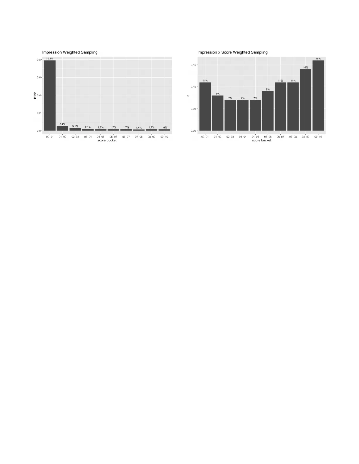
Surrogate-Based Pre valence Measurement for Large-Scale A/B T esting Zehao Xu Pinterest, Inc. T oronto, ON, Canada zehaoxu@pinterest.com T ony Paek Pinterest, Inc. New Y ork, NY, USA tpaek@pinterest.com Ke vin O’Sullivan Pinterest, Inc. New Y ork, NY, USA kosullivan@pinterest.com Attila Dobi Pinterest, Inc. San Francisco, CA, USA adobi@pinterest.com Abstract Online media platforms often need to measure how frequently users are exposed to sp ecic content attributes in order to evaluate trade- os in A/B experiments. A direct approach is to sample content, label it using a high-quality rubric ( e.g., an e xpert-reviewed LLM prompt), and estimate impression-w eighted prevalence. Ho wever , repeatedly running such lab eling for ev ery experiment arm and segment is too costly and slow to serve as a default measurement at scale. W e present a scalable surrogate-based prevalence measurement framework that decouples expensive labeling from p er-experiment evaluation. The framework calibrates a surrogate signal to reference labels oine and then uses only impr ession logs to estimate pre val- ence for arbitrary experiment arms and segments. W e instantiate this framework using scor e bucketing as the surr ogate: we discretize a model score into buckets, estimate bucket-lev el prevalences from an oine labele d sample, and combine these calibrated bucket level prevalences with the bucket distribution of impressions in each arm to obtain fast, log-based estimates. Across multiple large-scale A/B tests, w e validate that the sur- rogate estimates closely match the reference estimates for both arm-level prevalence and treatment–control deltas. This enables scalable, low-latency pre valence measurement in experimentation without requiring per-experiment labeling jobs. Ke ywords Content- Attribute Measurement , LLM-Labeling, Prevalence Es- timation, ML-Score Surrogate, A/B testing, Scalable Measurement, Calibration A CM Reference Format: Zehao Xu, T ony Paek, Kevin O’Sullivan, and Attila Dobi. 2026. Surrogate- Based Prevalence Measurement for Large-Scale A/B T esting. In Proceedings Permission to make digital or hard copies of all or part of this work for personal or classroom use is granted without fee provided that copies are not made or distributed for prot or commercial advantage and that copies bear this notice and the full citation on the rst page. Copyrights for components of this work owned by others than the author(s) must be honor ed. Abstracting with cr edit is permitted. T o copy otherwise, or republish, to post on servers or to redistribute to lists, requires prior specic permission and /or a fee. Request p ermissions from permissions@acm.org. KDD ’26, Jeju, Korea © 2026 Copyright held by the owner/author(s). Publication rights licensed to A CM. ACM ISBN 978-x-xxxx-xxxx-x/Y YY Y/MM https://doi.org/XXXXXXX.XXXXXXX of The 32nd A CM SIGKDD Conference on Knowledge Discovery and Data Min- ing (KDD ’26) . ACM, New Y ork, NY, USA, 8 pages. https://doi.org/XXXXXXX. XXXXXXX 1 Introduction Modern recommender systems and media platforms must balance user engagement against the need to manage exposure to certain content attributes. T eams often summarize such exposure objectives in terms of prevalence : the fraction of impressions associated with a given target category . At the same time, product decisions are largely driven by large-scale A/B experiments [ 8 ], where variants adjust ranking or ltering and are e valuated on both engagement and attribute-specic exposure metrics. One way to measure prevalence is to sample contents from trac, label it with LLMs using expert-validated prompts, and apply an es- timation. In our setting, we use PPSW OR (probability-proportional- to-size without replacement) sampling [ 7 ] and the Hansen–Hurwitz estimator [6] to obtain high-quality and unbiased measurements. Howev er , directly using LLM-based pr evalence as a default met- ric for every experiment is impractical. Running a separate LLM job per arm and p er segment is expensive, and quickly be comes infeasible on a platform with hundreds of concurrent experiments. Moreover , experimenters often care about relatively small but mean- ingful changes in prevalence. A single LLM measurement per arm tends to emphasize the absolute level, so many small treatment– control deltas appear statistically non-signicant. Running LLM labeling per experiment, per segment, and per day to address this would further amplify cost and latency . W e address these challenges with a ML-score surrogate method that reuses a single LLM-based calibration of model scores across many experiments. W e discretize model scores into buckets, es- timate bucket-level prevalences fr om an oine calibration sample, and then combine these with the observed distribution of impres- sions ov er buckets in each experiment arm to obtain fast, log-based prevalence estimates. W e integrate this method into a large-scale experiment platform, and augment it with a day-level aggregation that focuses on treatment and control delta, improving sensitivity to small shifts. Our approach is closely related to surrogate-outcome methods, where the quantity of interest is not directly obser ved but inferred using an intermediate signal [ 1 ]. Such methods are commonly used KDD ’26, August 9–13, 2026, Jeju, K orea Zehao Xu, T ony Paek, Kevin O’Sullivan, and Aila Dobi when long-run outcomes are costly or slo w to measure in experi- ments, and only short-run outcomes ar e readily observed. In our setting, direct daily LLM-based pr evalence measurement is accurate but operationally impractical; the ML-score therefore serves as a surrogate for pre valence. A key advantage of our setting is that we can directly validate surrogate quality by comparing surrogate- based estimates to LLM-based pre valence estimates on the same experiments. 2 Prevalence Estimation W e consider the problem of estimating the prevalence of a categor y 𝑘 on a large-scale me dia platform. Let K = { Food-Re cipe , Lawn and Garden , Gen- AI Generated , . . . } denote the set of content-attributes considered in this study , and x a particular 𝑘 ∈ K . Our target quantity is the prevalence of category 𝑘 within 𝑆 – which can denote the full population or a specic subset such as an experiment arm (control, tr eatment), a user demographic (country , age), an app surface, or intersections of these. The engineering details of our production pre valence pipeline are described in Farooq et al. [ 5 ]. In this section, we briey recap the core estimator and introduce notation that we will use throughout the rest of the paper , in particular when we describe the ML-score surrogate method and its calibration. 2.1 Notation W e consider a large population of content items, indexed by 𝑖 = 1 , . . . , 𝑁 . For each item 𝑖 , we obser ve: • 𝐼 𝑖 : the total number of impressions of item 𝑖 over a given time window . • 𝑍 𝑖 ,𝑘 ∈ { 0 , 1 } : a label indicating whether item 𝑖 is truly in category 𝑘 ( 1 ) or not ( 0 ). For a given segment 𝑆 , let D ( 𝑆 ) ⊆ { 1 , . . . , 𝑁 } denote the set of items that receive impressions from 𝑆 , and let 𝐼 𝑖 ( 𝑆 ) be the number of impressions of item 𝑖 from 𝑆 over the time windo w of interest. The total impressions of item 𝑖 satisfy 𝐼 𝑖 = Í 𝑆 𝐼 𝑖 ( 𝑆 ) . The prevalence of category 𝑘 in segment 𝑆 can be written as: P 𝑘 ( 𝑆 ) = P ( 𝑍 𝑘 = 1 | impressions ∈ 𝑆 ) = Í 𝑖 ∈ D ( 𝑆 ) 𝑍 𝑖 ,𝑘 𝐼 𝑖 ( 𝑆 ) Í 𝑖 ∈ D ( 𝑆 ) 𝐼 𝑖 ( 𝑆 ) , (1) When 𝑆 is the entire population, D ( 𝑆 ) = { 1 , . . . , 𝑁 } and 𝐼 𝑖 ( 𝑆 ) = 𝐼 𝑖 , recovering the global pre valence denition. 2.2 Sampling Design and Hansen–Hur witz Estimator Directly labeling all items in D ( 𝑆 ) (often billions of items across many segments) is infeasible, so we estimate these quantities from a sample. W e adopt a PPSW OR design, in which items are sampled with probabilities proportional to a chosen size measure. Compared with simple random sampling, PPSW OR allows us to oversample items that are more informative (e.g., high-impression items), achiev- ing similar statistical power with a much smaller sample size. For category 𝑘 and segment 𝑆 , each item 𝑖 ∈ D ( 𝑆 ) is assigned a sampling weight 𝑤 𝑖 ,𝑘 ( 𝑆 ) ∝ 𝑓  𝐼 𝑖 ( 𝑆 )  , (2) and is selected into the sample with probability 𝑝 sample , 𝑖 ,𝑘 ( 𝑆 ) = 𝑤 𝑖 ,𝑘 ( 𝑆 ) Í 𝑗 ∈ D ( 𝑆 ) 𝑤 𝑗 ,𝑘 ( 𝑆 ) . (3) Here 𝑓 is a function of impressions; it can be 𝐼 𝑖 ( 𝑆 ) itself, or a com- bination such as 𝐼 𝑖 ( 𝑆 ) multiplied by other factors (e.g., mo del score). W e discuss concrete choices of 𝑓 in more detail in Section 5.1. Suppose we draw a sample of size 𝑛 from D ( 𝑆 ) and obtained sampled indices { 𝑖 1 , . . . , 𝑖 𝑛 } . The Hansen–Hurwitz estimator for the total target-category impressions in 𝑆 is b 𝑇 𝑘 ( 𝑆 ) = 1 𝑛 𝑛  𝑡 = 1 𝑍 𝑖 𝑡 ,𝑘 𝐼 𝑖 𝑡 ( 𝑆 ) 𝑝 sample , 𝑖 𝑡 ,𝑘 ( 𝑆 ) . (4) The prevalence in segment 𝑆 is then estimated as b P 𝑘 ( 𝑆 ) = b 𝑇 𝑘 ( 𝑆 ) Í 𝑗 ∈ D ( 𝑆 ) 𝐼 𝑗 ( 𝑆 ) . (5) In practice, both Í 𝑗 ∈ D ( 𝑆 ) 𝐼 𝑗 ( 𝑆 ) and Í 𝑗 ∈ D ( 𝑆 ) 𝑤 𝑗 ,𝑘 ( 𝑆 ) are com- puted directly from the underlying logs for segment 𝑆 . 2.3 W eighte d Reservoir Sampling T o eciently draw a PPSW OR sample at scale, we use weighted random sampling with a reser voir [ 4 ]. Each item 𝑖 is assigned an index 𝑈 1 / 𝑤 𝑖 ,𝑘 ( 𝑆 ) 𝑖 , (6) where 𝑈 𝑖 ∼ Uniform ( 0 , 1 ) and 𝑤 𝑖 ,𝑘 ( 𝑆 ) is the sampling weight. The 𝑛 items with the largest index are selected into the sample. This procedure implements PPSW OR in a single streaming pass, without the need to know 𝑁 in advance. 2.4 LLM Labeling A central design choice in our prevalence pipeline is the source of “ground-truth” lab els for whether an item belongs to a category 𝑘 ∈ K . In principle, there are three broad options: • Heuristic or rule-based labels (including model-score thresholds). For example, one might classify an item as pos- itive if its category-specic score exceeds a xe d threshold. This approach is easy to deplo y , but generally the model’s precision and recall are often not sucient to ser ve as a reference standard , especially when policies evolve. More fundamentally , any measurement that reuses the same sig- nals or thresholds that are already used for enforcement risks “grading our own homework” and systematically under es- timating true prevalence [9]. • Human expert annotations (specialists or trained raters), which provide very high quality labels but do not scale: ob- taining tens of thousands of fresh lab els per categor y would be prohibitively slow and costly [13]. • LLM-based labeling (prompted large language models, optionally with expert-review ed prompts and calibration), which oers a pragmatic middle ground: substantially higher delity than simple heuristics or raw score thresholds, at a fraction of the cost and latency of full human annotation. As Surrogate-Based Prevalence Measurement for Large-Scale A/B T esting KDD ’26, August 9–13, 2026, Jeju, K orea a result, prompted LLMs are increasingly used as scalable labelers/judges in practice [10, 12, 15]. For each sampled item 𝑖 , the LLM produces a binary label 𝑍 𝑖 ,𝑘 ∈ { 0 , 1 } , where 𝑍 𝑖 ,𝑘 = 1 indicates that the item is judged to b elong to category 𝑘 , and 𝑍 𝑖 ,𝑘 = 0 otherwise. Substituting these labels into the Hansen–Hur witz estimator (4) and the prevalence formula (5) yields an unbiased estimate of category prevalence for the platform or for any base population over which the sampling is dened. In practice, we use this LLM- based estimator as the reference standard against which we calibrate our ML-score surrogate method in Section 4. 3 Methodology: ML Score Surrogate Prevalence The LLM-based estimator provides high-quality measur ements of category prevalence, but it r equires running an LLM labeling job whenever we want a new estimate . This is acceptable for a small number of global or on-demand studies, but becomes problematic when we attempt to use prevalence as a default experiment metric at scale—for example, to (i) measure prevalence deltas for many experiments per day , or (ii) estimate prevalence dierences across multiple user or trac segments within a single experiment. There are two main challenges. Cost. Even a one-time measurement with a sample of roughly tens of thousands items can incur non-trivial lab eling cost. Scaling this approach to millions of items across many experiments and segments quickly becomes prohibitively expensive. Latency . W e support both real-time and batch ( bulk) LLM la- beling. Real-time labeling is signicantly more expensive per item than bulk labeling, while bulk jobs typically take on the order of 10–24 hours from submission to completion. With many concurrent experiments and segments, end-to-end latency can b e even longer , and heavy usage can also stress LLM API capacity and stability . These limitations motivate the nee d for an alternative approach that can: • avoid per-experiment LLM labeling, • provide low-latency estimates suitable for always-on monit- oring, and • scale to many experiments and segments at near-log-query cost. T o address this, we adopt a surrogate-based measurement ap- proach that decouples expensive labeling from per-experiment eval- uation. In this paper w e instantiate the surrogate using model-score bucketing, yielding a score-bucket proxy prevalence estimator that can be computed from impression logs for arbitrar y cohorts at query time. 3.1 Bucket-Level Pre valence Let 𝑚 𝑖 ,𝑘 ∈ [ 0 , 1 ] be the model score for categor y 𝑘 on item 𝑖 ; higher values indicate that item 𝑖 is more likely to be true in categor y 𝑘 . W e discretize the model scores for into 𝐵 buckets: B = { 𝑏 1 , . . . , 𝑏 𝐵 } , where each bucket 𝑏 𝑗 corresponds to an interval 𝑏 1 = [ 𝑢 0 , 𝑢 1 ) , 𝑏 2 = [ 𝑢 1 , 𝑢 2 ) , . . . , 𝑏 𝐵 = [ 𝑢 𝐵 − 1 , 𝑢 𝐵 ] , with 0 = 𝑢 0 < 𝑢 1 < · · · < 𝑢 𝐵 − 1 < 𝑢 𝐵 = 1 . For a given segment 𝑆 and category 𝑘 , we dene the bucket-level prevalence as P 𝑘 ,𝑏 ( 𝑆 ) = P ( 𝑍 𝑘 = 1 | 𝑚 𝑘 ∈ 𝑏 , impression ∈ 𝑆 ) , (7) i.e., the probability that impressions from segment 𝑆 are truly in category 𝑘 , conditional on model score 𝑚 𝑘 falling in bucket 𝑏 . 3.2 Prevalence Estimation and V ariance Propagation Let 𝑐 𝑘 ,𝑏 ( 𝑆 ) denote the share of impressions from 𝑆 whose mo del scores for category 𝑘 fall into bucket 𝑏 : 𝑐 𝑘 ,𝑏 ( 𝑆 ) = P ( 𝑚 𝑘 ∈ 𝑏 | impression ∈ 𝑆 ) = Impressions in 𝑆 with 𝑚 𝑘 ∈ 𝑏 T otal Impressions in 𝑆 , (8) so that Í 𝑏 ∈ B 𝑐 𝑘 ,𝑏 ( 𝑆 ) = 1 . Using the law of total probability , we estimate the prevalence of category 𝑘 in segment 𝑆 as: b P 𝑘 ( 𝑆 ) =  𝑏 ∈ B 𝑐 𝑘 ,𝑏 ( 𝑆 ) · b P 𝑘 ,𝑏 ( 𝑆 ) . (9) In practice, the calibration b P 𝑘 ,𝑏 ( 𝑆 ) is usually performed once on a large “global” segment (i.e., all trac), and the resulting bucket- level estimates b P 𝑘 ,𝑏 are then reused acr oss segments 𝑆 . There are several reasons for this design: (1) Stability of bucket-level prevalences. In our oine com- parisons, the values of b P 𝑘 ,𝑏 ( 𝑆 ) are typically much more strongly determined by the categor y 𝑘 and bucket 𝑏 than by the segment 𝑆 . Empirically , for a xed ( 𝑘 , 𝑏 ) , the bucket-le vel prevalences are fairly stable acr oss a wide range of segments. (2) Focus on distributional shifts. When we estimate the change in prevalence for a specic segment 𝑆 across experi- ment arms, we hold the calibrated b P 𝑘 ,𝑏 xed and attribute dierences in b P 𝑘 ( 𝑆 ) to shifts in the impression-share dis- tribution 𝑐 𝑘 ,𝑏 ( 𝑆 ) . Under this view , using segment-specic calibrations b P 𝑘 ,𝑏 ( 𝑆 ) vs. a global b P 𝑘 ,𝑏 has limited impact on detecting deltas between arms. Therefore, w e approximate the segment-lev el prevalence as b P 𝑘 ( 𝑆 ) ≈  𝑏 ∈ B 𝑐 𝑘 ,𝑏 ( 𝑆 ) · b P 𝑘 ,𝑏 . (10) Intuitively , (10) is a buckete d approximation to Equation (1): we treat the bucket-level prevalences as a learned “score → likelihood” mapping, and then reweight by the score-bucket distribution of impressions in segment 𝑆 . Also, we can assume the bucket-level estimators ar e approxim- ately independent acr oss 𝑏 (reasonable given disjoint buckets), then applying standard variance propagation to (10) yields: V ar  b P 𝑘 ( 𝑆 )  ≈  𝑏 ∈ B 𝑐 𝑘 ,𝑏 ( 𝑆 ) 2 V ar  b P 𝑘 ,𝑏  . (11) KDD ’26, August 9–13, 2026, Jeju, K orea Zehao Xu, T ony Paek, Kevin O’Sullivan, and Aila Dobi 4 Experimental Results T o validate the ML-score surrogate method in a realistic setting, we compare it against the LLM-based prevalence estimator on several production experiments. In each case, we treat the LLM- based prevalence (Section 2) as the reference , and evaluate how well the surrogate recov ers both: (i) the absolute prevalence levels in each arm, and (ii) the between-group deltas. 4.1 Experiment A: T arget-Category Filtering Our rst validation uses a production A/B experiment that applies additional ltering for two target categories, 𝑘 1 and 𝑘 2 , on a major recommendation surface. The goal is to evaluate how aggr essive ltering of these categories aects user experience and engagement. The experiment includes three arms: • Control: baseline production settings. • Treatment 1 : baseline settings plus additional ltering for category 𝑘 1 , removing items with 𝑚 𝑖 ,𝑘 1 ≥ 0 . 70 1 . • Treatment 2 : baseline settings plus additional ltering for category 𝑘 2 , removing items with 𝑚 𝑖 ,𝑘 2 ≥ 0 . 10 . The null hypotheses are that ltering on 𝑘 ℓ for ℓ ∈ { 1 , 2 } do not reduce prevalences. For each arm, we estimate the pre valences by: (1) LLM-based estimator (reference): impression-weighted sampling, i.e., 𝑤 𝑖 ,𝑘 ( 𝑆 ) ∝ 𝐼 𝑖 ( 𝑆 ) , and LLM labeling for each arm. (2) ML-score surrogate estimator: using the calibrated bucket prevalences b P 𝑘 ℓ , 𝑏 for each category 𝑘 ℓ and bucket 𝑏 , together with the arm-specic impression shares 𝑐 𝑘 ℓ , 𝑏 ( Control ) and 𝑐 𝑘 ℓ , 𝑏 ( Treatment ℓ ) , aggregated according to Equation (10) . In this experiment we use 𝐵 = 10 equally spaced buckets with boundaries 0 = 𝑢 0 < 𝑢 1 = 0 . 1 < · · · < 𝑢 9 = 0 . 9 < 𝑢 10 = 1 . 0 . Figure 1 shows the impression-share distributions 𝑐 𝑘 ℓ , 𝑏 ( Control ) (salmon) and 𝑐 𝑘 ℓ , 𝑏 ( Treatment ℓ ) (cyan) over score buckets across the entire experiment window for categories 𝑘 1 and 𝑘 2 , under the given thresholds, respectively . By denition, Í 𝑏 ∈ B 𝑐 𝑘 ℓ , 𝑏 ( 𝑆 ) = 1 for each segment 𝑆 ∈ { Control , Treatment ℓ } , so each panel can be interpreted as a normalized histogram of where impressions fall in score space. Be cause most impressions lie in the lowest-score bucket [ 0 , 0 . 1 ) , the main panels are dominated by that bar; we therefor e add zoomed-in insets over the higher-score regions. In these insets, for scores above 0 . 7 in the treatment 1 arm (left) and ab ove 0 . 1 in the treatment 2 arm (right), both treatments allocate substantially fewer impressions than control, illustrating how the thresholds shift impression mass away from higher-score buckets. T able 1 summarizes the prevalence estimates b P 𝑘 ℓ ( Control ) and b P 𝑘 ℓ ( Treatment ℓ ) . • For 𝑘 1 , the treatment reduces prevalence from approximately 3.6% to 2.9% (around 19.4% reduction) under the LLM-based estimator and from 3.8% to 2.8% (26.3% reduction) under the ML-scor e surrogate , corr esponding to treatment–control deltas of 0.70% and 1.03%, respectively . • For 𝑘 2 , the treatment reduces prevalence from about 1.3% to 1.0% (LLM; 23% drop) and from 1.4% to 0.9% (Surrogate; 35.7% drop), with deltas of 0.31% and 0.49%. 1 All thresholds, prevalence values, statistical summaries and are illustrative and have been modied for condentiality. They do not r epresent actual platform metrics. T able 1: Comparison of LLM-based vs. ML-score surrogate prevalence in Exp eriment A for categories 𝑘 1 and 𝑘 2 . The ranges denote 95% condence inter vals Metric LLM-based. ML-score surrogate. b P 𝑘 1 ( Control ) 3.61% [3.40%, 3.82%] 3.81% [3.67%, 3.95%] b P 𝑘 1 ( Treatment 1 ) 2.91% [2.72%, 3.10%] 2.78% [2.64%, 2.92%] Δ 𝑘 1 , Treat 1 − Ctrl − 0 . 70% − 1 . 03% 𝑝 value 0 . 00 ( Stats-Sig ) 0 . 00 ( Stats-Sig ) b P 𝑘 2 ( Control ) 1.32% [1.20%, 1.43%] 1.36% [1.20%, 1.52%] b P 𝑘 2 ( Treatment 2 ) 1.01% [0.91%, 1.11%] 0.87% [0.70%, 1.04%] Δ 𝑘 2 , Treat 2 − Ctrl − 0 . 31% − 0 . 49% 𝑝 value 0 . 00 ( Stats-Sig ) 0 . 00 ( Stats-Sig ) In all cases, the surrogate estimates lie within the 95% condence intervals of the LLM-based reference, and the inferr ed treatment eects are statistically signicant and closely aligned in both sign and magnitude. 4.2 Experiment B: UI-Only Change with No Expected Prevalence Shift Our se cond validation focuses on a user-interface refr esh where we do not expect any change in category 𝑘 1 and 𝑘 2 prevalence. The experiment updates the web ov erow menu by modifying the hide/report icon to align with industr y-standard visuals, without altering the underlying functionality or ranking logic. Therefore , the pre-registered hypothesis is that this UI change should not ae ct prevalence. This experiment tests whether the ML-score surrogate can detect a null eect and agree with the LLM-based estimator when no true prevalence shift is present. T able 2 summarizes the prevalence estimates over the whole experiment window . For 𝑘 1 , the control and treatment arms have very similar prevalences: 3.44% vs. 3.31% under the LLM-base d estimator and 3.39% vs. 3.40% under the ML-score surrogate. For 𝑘 2 , the prevalences are likewise close: 1.32% vs. 1.40% (LLM) and 1.39% vs. 1.35% (surr ogate), with treatment–control deltas near zero in all cases. The surrogate estimates lie within the 95% condence intervals of the LLM-based reference, and none of the inferred treatment eects are statistically signicant, consistent with the experimental hypothesis. 5 Implementation W e now discuss ho w the ML-score surrogate metho dology is imple- mented in practice. The implementation has two main comp onents: (1) an oine calibration pipeline that p eriodically produces bucket- level pre valences b P 𝑘 ,𝑏 from LLM labels, and (2) an online integration with the experiment platform that uses these calibrations, together with impression logs, to estimate prevalence for arbitrary experiments and segments. 5.1 O line Calibration Pip eline T o estimate bucket-level prevalences { P 𝑘 ,𝑏 } 𝑏 ∈ B and associate d variances { V ar ( b P 𝑘 ,𝑏 ) } 𝑏 ∈ B , a natural baseline is to use stratied Surrogate-Based Prevalence Measurement for Large-Scale A/B T esting KDD ’26, August 9–13, 2026, Jeju, K orea Figure 1: Bucket-level impression-share shifts for categories 𝑘 1 and 𝑘 2 in Experiment A. The treatment arm reduces exposure primarily by shifting impressions out of higher score buckets. T able 2: Comparison of LLM-based vs. ML-score surrogate prevalence for categories 𝑘 1 and 𝑘 2 in Experiment B. Metric LLM-based ML-score surrogate b P 𝑘 1 ( Control ) 3.44% [3.23%, 3.64%] 3.39% [3.25%, 3.53%] b P 𝑘 1 ( Treatment ) 3.31% [3.11%, 3.51%] 3.40% [3.26%, 3.53%] Δ 𝑘 1 , Treat − Ctrl − 0 . 13% 0 . 01% 𝑝 value 0 . 38 ( No Stats-Sig ) 0 . 95 ( No Stats-Sig ) b P 𝑘 2 ( Control ) 1.32% [1.19%, 1.45%] 1.39% [1.22%, 1.56%] b P 𝑘 2 ( Treatment ) 1.40% [1.26%, 1.53%] 1.35% [1.18%, 1.52%] Δ 𝑘 2 , Treat − Ctrl − 0 . 07% − 0 . 04% 𝑝 value 0 . 40 ( No Stats-Sig ) 0 . 67 ( No Stats-Sig ) sampling : treat each bucket 𝑏 as a separate stratum (or segment 𝑆 = 𝑏 ) and apply the Hansen–Hur witz estimator on a bucket- specic sample . This design can giv e direct contr ol over the number of labeled examples per bucket. Howev er , in practice, drawing and labeling a separate sample for every bucket and category is operationally expensive and dicult to scale. Instead, our calibration pipeline constructs a single global sample and reuses it to estimate prevalences for many segments 𝑆 , including (as a special case) the score buckets themselves. In particular , for each bucket 𝑏 ∈ B we dene the segment 𝑆 = 𝑏 as the set of impressions whose mo del score 𝑚 𝑖 ,𝑘 falls in bucket 𝑏 , and estimate the bucket-level pr evalence by applying the same estimator with 𝑆 = 𝑏 : b P 𝑘 ,𝑏 = b P 𝑘 ( 𝑆 = 𝑏 ) . (12) (1) Global sample. Over a calibration window , draw a global PPSW OR sample of items { 𝑖 1 , . . . , 𝑖 𝑛 } using weighted reser- voir sampling with inclusion pr obabilities 𝑝 sample , 𝑖 ,𝑘 , which is the probability that item 𝑖 is selected into this global calib- ration sample. (2) Joint probability . Let 𝐼 𝑖 ( 𝑏 ) be the number of impressions of item 𝑖 arising from bucket 𝑏 in the calibration window , and let ⊮ 𝑖 ∈ 𝑏 be the indicator that item 𝑖 receives at least one impression from 𝑏 . Using the global sample { 𝑖 1 , . . . , 𝑖 𝑛 } , we estimate the joint probability that an impression is both in category 𝑘 and in bucket 𝑏 as b P  𝑍 𝑖 ,𝑘 = 1 ∩ impression ∈ 𝑏  = 1 𝑛 𝑛  𝑡 = 1 𝑍 𝑖 𝑡 ,𝑘 ⊮ 𝑖 𝑡 ∈ 𝑏 𝐼 𝑖 𝑡 ( 𝑏 ) 𝑝 sample , 𝑖 𝑡 ,𝑘 . (13) (3) Bucket-level prevalence. W e also have access to the mar- ginal probability that a random impression belongs to bucket 𝑏 , which can be computed directly from logs as P ( impression ∈ 𝑏 ) = Í 𝑖 ∈ D ( 𝑏 ) 𝐼 𝑖 ( 𝑏 ) Í 𝑖 ∈ D 𝐼 𝑖 . (14) By the denition of conditional probability , the estimated prevalence of category 𝑘 in bucket 𝑏 is b P 𝑘 ( 𝑆 = 𝑏 ) = b P ( 𝑍 𝑘 = 1 | impressions ∈ 𝑏 ) = b P  𝑍 𝑖 ,𝑘 = 1 ∩ impression ∈ 𝑏  P ( impression ∈ 𝑏 ) , (15) A practical challenge is that model scores are highly skewed toward low values. If we used impressions alone as weights, i.e., 𝑤 𝑖 ,𝑘 ∝ 𝐼 𝑖 , the resulting score distribution in the sample would b e dominated by the lowest bucket ( 0 , 0 . 1 ] : in our data, as Figure 2 (a), roughly 80% of sampled impressions fall into this bucket, while buckets with larger scores ( e.g., 𝑚 𝑖 ,𝑘 > 0 . 3 ) each contain only about 2% of the mass. With a sample of 10 , 000 items, fewer than 200 would lie in each higher bucket, limiting statistical power for estimating P 𝑘 ,𝑏 at the upper end of the score range. Using model score as auxiliary information [ 14 ], i.e., 𝑤 𝑖 ,𝑘 ∝ 𝐼 𝑖 𝑚 𝑖 ,𝑘 , mitigates this issue by b oosting the inclusion probability of higher-score items. On the same underlying dataset, as illustrated in Figure 2 (b), this design yields a much more balanced bucket distribution: every bucket has at least ∼ 7% of the sample, and the ( 0 . 9 , 1 ] buckets account for roughly 16% each. This improves the statistical power of higher bucket-level pre valence estimates with minimal operational overhead. 5.2 Online Integration 5.2.1 Deterministic SQL Metric. For integration with the experi- ment platform, we rst implement a deterministic end-to-end SQL metric. The key idea is that the platform lls in a small set of para- meters for each experiment and runs a single SQL query that: (1) reads the latest calibration table { b P 𝑘 ,𝑏 } 𝑏 ∈ B , KDD ’26, August 9–13, 2026, Jeju, K orea Zehao Xu, T ony Paek, Kevin O’Sullivan, and Aila Dobi (a) Impression-weighted sampling ( 𝑤 𝑖 ,𝑘 ∝ 𝐼 𝑖 ). (b) Impression × score sampling ( 𝑤 𝑖 ,𝑘 ∝ 𝐼 𝑖 𝑚 𝑖 ,𝑘 ). Figure 2: Comparison of score-bucket distributions under two sampling schemes. Left: sampling with weights proportional to impressions alone produces a very low-score-heavy sample, leaving few examples in high-score buckets. Right: sampling with weights proportional to impression × model score yields a more balanced distribution across buckets, improving the precision of bucket-level prevalence estimates. (2) pulls model scores of category 𝑘 and daily impression logs for the experiment arms, (3) aggregates impressions to obtain bucket-level shares 𝑐 𝑘 ,𝑏 ( 𝑆 ) per arm per day , and (4) computes arm-level prevalences and condence inter vals analytically . For a given experiment, the metric is parameterized by: • Inputs: – exp_name , exp_version , – day 𝑑 , – experiment groups (e.g., control , treatment ). • Implementation: the experiment platform populates these variables into a templated SQL quer y , then executes the query once per experiment p er segment per day . • Outputs: – daily b P 𝑘 ( 𝑆 ; 𝑑 ) per arm, – condence inter vals per arm (derived from V ar ( b P 𝑘 ( 𝑆 ; 𝑑 ) ) ), – arm-level dierences Δ ( 𝑑 ) = b P 𝑘 ( treatment; 𝑑 ) − b P 𝑘 ( control; 𝑑 ) , 𝑑 = 1 , . . . , 𝐷 , and associated 𝑧 -scores and 𝑝 -values. 5.2.2 Simulation-Based Extensions. If a purely deterministic SQL implementation is infeasible, or if we wish to express pr evalence as a user-level metric, we can add a simulation layer on top of the score-bucket calibration. Algorithm 1 shows how; for a given day 𝑑 , (1) we draw one calibrate d prevalence P ★ 𝑘 ,𝑏 per score bucket from the logit-normal calibration, (2) simulate which impressions are agged at the impression level, and (3) aggregate to obtain daily prevalence estimates for the control and treatment arms. In Step 1, we convert the bucket-level estimate and variation into a logit-normal distribution and draw a single P ★ 𝑘 ,𝑏 per bucket. In Steps 2–4, we attach these P ★ 𝑘 ,𝑏 values to the impression logs, run a Monte Carlo simulation at the impression level, and aggregate by user and group to obtain day- 𝑑 prevalences b P 𝑘 ( control ; 𝑑 ) and b P 𝑘 ( treatment ; 𝑑 ) . In practice, this yields good point estimates for each arm per category p er day 6 Discussion W e conclude by discussing two practical questions that arose in deploying the ML-score surrogate method: (i) how to interpret and claim wins for small prevalence shifts in experiments, and (ii) how to choose an appropriate bucketization of model scores. 6.1 Detecting Small Shifts with Statistical Power 6.1.1 Calibration-Dominated Uncertainty in A rm-Level Estimates. The variability of the ML-score surrogate estimates has two con- ceptually distinct components: (1) Global calibration variation at the bucket level, captured by V ar ( b P 𝑘 ,𝑏 ) , and (2) Experiment-level variation in bucket mixes 𝑐 𝑘 ,𝑏 ( 𝑆 ) across arms and days. With a suciently large calibration sample (e.g., millions of labeled items per bucket), the calibration variation could be made negligible. In practice, however , our calibration budget is constrained by LLM labeling cost, so we work with much smaller bucket-wise samples. Under these realistic calibration sizes, our analytic vari- ance is dominated by the bucket-level calibration variation. As a result, the corresponding condence intervals for b P 𝑘 ( control ) and b P 𝑘 ( treatment ) are b est interpreted as answering: “If we repeated the global LLM calibration many times, where would the absolute prevalence for this arm lie?” Surrogate-Based Prevalence Measurement for Large-Scale A/B T esting KDD ’26, August 9–13, 2026, Jeju, K orea Algorithm 1 ML-score surrogate Prevalence (Single Calibration Draw) 1: input: day 𝑑 ; category 𝑘 ; user 𝑢 ; item 𝑖 and its model score 𝑚 𝑖 ,𝑘 ; calibration table { b P 𝑘 ,𝑏 , V ar ( b P 𝑘 ,𝑏 ) } 𝑏 ∈ B ; impression logs imp 𝑑 , 𝑢,𝑖 ; experiment groups 𝑔 ( 𝑢 ) ∈ { control , treatment } 2: output: daily prevalences b P 𝑘 ( control ; 𝑑 ) , b P 𝑘 ( treatment ; 𝑑 ) , and daily eect Δ ( 𝑑 ) 3: /* Step 1: draw one calibrated prevalence per bucket */ 4: for each bucket 𝑏 ∈ B do 5: 𝜇 𝑘 ,𝑏 ← ln  b P 𝑘 ,𝑏 / ( 1 − b P 𝑘 ,𝑏 )  6: 𝜎 𝑘 ,𝑏 ←  V ar ( b P 𝑘 ,𝑏 )   b P 𝑘 ,𝑏 ( 1 − b P 𝑘 ,𝑏 )  ⊲ Delta-Method [11] variance on logit scale 7: draw 𝑧 𝑘 ,𝑏 ∼ N ( 0 , 1 ) ⊲ e.g., Box–Muller [2] 8: 𝜃 𝑘 ,𝑏 ← 𝜇 𝑘 ,𝑏 + 𝜎 𝑘 ,𝑏 𝑧 𝑘 ,𝑏 9: P ★ 𝑘 ,𝑏 ← exp ( 𝜃 𝑘 ,𝑏 ) /  1 + exp ( 𝜃 𝑘 ,𝑏 )  10: /* Step 2: attach buckets and P ★ 𝑘 ,𝑏 to impressions */ 11: for each log entr y ( 𝑢, 𝑖 ) on day 𝑑 do 12: 𝑏 ← bucket ( 𝑚 𝑖 ,𝑘 ) ⊲ map score to bucket 13: 𝐼 𝑑 , 𝑢,𝑖 ← Í imp 𝑑 , 𝑢,𝑖 ⊲ aggregate impressions of item 𝑖 for user 𝑢 14: attach P ★ 𝑘 ,𝑏 to ( 𝑑 , 𝑢 , 𝑖 ) 15: /* Step 3: simulate target-category impressions per user */ 16: for each user 𝑢 do 17: 𝐼 𝑑 , 𝑢 ← Í 𝑖 𝐼 𝑑 , 𝑢,𝑖 18: V 𝑑 , 𝑢 ← 0 ⊲ target-category impressions of item for user 𝑢 19: for each item 𝑖 shown to user 𝑢 on day 𝑑 do 20: for 𝑡 = 1 to 𝐼 𝑑 , 𝑢,𝑖 do ⊲ loop over impressions of 𝑖 21: draw 𝑟 ∼ Uniform ( 0 , 1 ) 22: if 𝑟 < P ★ 𝑘 , bucket ( 𝑖 ) then 23: 𝑉 𝑑 , 𝑢 ← 𝑉 𝑑 , 𝑢 + 1 24: /* Step 4: aggregate to group-level prevalences */ 25: for each group 𝑔 ∈ { control , treatment } do 26: 𝐼 𝑑 ,𝑔 ← Í 𝑢 : 𝑔 ( 𝑢 ) = 𝑔 𝐼 𝑑 , 𝑢 27: 𝑉 𝑑 ,𝑔 ← Í 𝑢 : 𝑔 ( 𝑢 ) = 𝑔 𝑉 𝑑 , 𝑢 28: b P 𝑘 ( 𝑔 ; 𝑑 ) ← 𝑉 𝑑 ,𝑔 / 𝐼 𝑑 ,𝑔 29: /* Step 5: daily eect */ 30: Δ ( 𝑑 ) ← b P 𝑘 ( treatment; 𝑑 ) − b P 𝑘 ( control; 𝑑 ) For exploratory experiments such as Experiment A (Se ction 4.1, used for diagnostic validation rather than launch decisions), where the intervention intentionally produces a large shift in the impres- sion share of the target categories, the calibration-driven uncer- tainty does not materially aect conclusions: the resulting pre- valence changes are large (e.g., 20% or more) and remain clearly detectable even under conservative uncertainty estimates. In most production settings, how ever , changes are e xpected to be more incremental because we must balance content-shifting objectives against user engagement and other product constraints. In these more subtle experiments, where a 2%–5% relativ e change in pre valence would already be meaningful, calibration uncertainty can dominate arm-level condence intervals and cause small but systematic treatment eects to appear statistically non-signicant when evaluated solely using absolute per-arm estimates. 6.1.2 Delta-Focused Inference via Day-Level Sign T ests. For eval- uating experiment impact, we are usually more interested in the dierence between arms than in their absolute levels. In that set- ting it is natural to focus on experiment-lev el variation. Concr etely , we rst compute daily prevalences and the associated daily eects Δ ( 𝑑 ) using the ML-score surrogate with a xed calibration snapshot. Then aggregates { Δ ( 𝑑 ) } 𝐷 𝑑 = 1 across days to produce: • an empirical 95% condence inter val [ Δ 0 . 025 , Δ 0 . 975 ] from the quantiles of { Δ ( 𝑑 ) } , and • a sign-test 𝑝 -value [ 3 ] based on the fraction of days where Δ ( 𝑑 ) is p ositive vs. negative or a normalized 𝑝 -value. • if signicant, the observed mean eect ¯ Δ is unlikely to be explained by random variation under the null hypothesis; otherwise, we fail to reject the null. This answers the question: “Given the experiment’s trac and a xed calibration, how precisely can we estimate the dierence between arms?” In our deployments, this approach has pro ven useful for detect- ing small but consistent shifts in prevalence, even when the per-arm absolute intervals are relatively wide due to calibration uncertainty . Consider an experiment (Experiment C) that targets a sub category of category 𝑘 1 . Because this subcategor y accounts for only a small fraction of the overall 𝑘 1 impression share , we expect any change in P 𝑘 1 to be modest but systematic. Using the LLM-based estimator aggregated over the entire ex- periment window , the estimated prevalences are: b P 𝑘 1 ( control ) = 3 . 83% [ 3 . 69% , 3 . 96% ] , and b P 𝑘 1 ( treatment ) = 3 . 67% [ 3 . 53% , 3 . 80% ] , with overlapping 95% condence inter vals and a two-sided 𝑝 -value ≈ 0 . 31 , no signicant change. Howev er , given the experimental design, a small shift in exposure to the target sub category is expecte d. Using the ML-score surrogate, we can compute daily deltas Δ ( 𝑑 ) . The av erage delta over the exper- iment window is around − 0 . 16% ; relative to a baseline pre valence of about 3 . 8% , this corresponds to a ∼ 4 . 1% relative r eduction. As shown in Figure 3, the daily relativ e reductions are consistently negative. Aggr egating the day-level deltas yields a 𝑝 -value close to 0 , indicating a statistically signicant shift at the experiment level. As a sanity check and to guard against false positives, we also apply the same day-level aggregation to Experiment B (Subsection 4.2), where no prevalence shift is expected. In that case, 𝑝 -value 𝑘 1 ≈ 0 . 75 and 𝑝 -value 𝑘 2 ≈ 0 . 25 , aligning with our expe ctations. 6.2 Choice of Score Buckets The ML-score surr ogate relies on a discretization of the model score into buckets B = { 𝑏 1 , . . . , 𝑏 𝐵 } , and the choice of bucketization has direct implications for both bias and variance. There are two main trade-os: (1) Bias vs. resolution. Fewer , wider buckets reduce variance in b P 𝑘 ,𝑏 but can blur meaningful dierences in the score– label relationship, esp ecially in regions where the conditional KDD ’26, August 9–13, 2026, Jeju, K orea Zehao Xu, T ony Paek, Kevin O’Sullivan, and Aila Dobi Figure 3: Relative prevalence reduction vs. calendar day for category 𝑘 1 in Experiment C. The values are consistently negative over the experiment window , and the day-level ag- gregation yields a statistically signicant 𝑝 -value. prevalence changes rapidly with the score. Conversely , many narrow buckets provide ner resolution but require more calibration labels per bucket and can increase variance. (2) Score distribution skew . On real platforms, model scores are typically highly skewed towar d low values. With equal- width buckets (e.g., ten buckets over [ 0 , 1 ] ), most impressions fall into the lowest bucket(s), leaving relatively few examples in the high-score tail. Without appropriate sampling (Sec- tion 5.1), this can lead to noisy estimates precisely in the buckets that contribute most to measuring changes induced by threshold-based interventions. In this work we adopted a simple default of 𝐵 = 10 equal-width buckets over [ 0 , 1 ] combined with impression × score weighted sampling to ensure that each bucket receives a sucient number of calibration labels. That said, alternative bucket schemes may b e appropriate in other settings. Examples include: • Non-uniform buckets, with ner resolution near decision thresholds or in the high-score tail, and coarser buckets in low-score regions where the conditional prevalence is approximately constant. • Relative-score (quantile) buckets, where buckets are dened by quantiles of the score distribution (e.g., deciles) rather than xed raw-score ranges. This yields roughly equal num- bers of items p er bucket, which can simplify calibration and help avoid buckets that are extremely sparse in terms of labeled items. Quantile-based buckets also tend to be more stable over time: while raw model scores may shift across days, the relative ordering (and hence the score quantiles) is often much more stable , making the calibration mor e robust. In future work we plan to explore adaptive bucketization strategies that better balance bias and variance under a xed calibration budget, while retaining the core advantages of the ML-score surrog- ate framework. More broadly , although we instantiate our surrogate using model-score buckets in this work, the surr ogate can repres- ent many types of content or context featur es beyond raw model score. The most appropriate choice of the surrogate depends on the application and operational constraints. 7 Future Outlook A key motivation for our approach is that large-scale LLM lab eling is currently too expensive to ser ve as a default metric for experi- ments. In the longer term, as LLM inference becomes cheaper and more tightly integrated into ser ving stacks, it may be come feasible to label much larger fractions of the corpus ( or e ven all content) for multiple content attributes. In that regime, the relative importance of our surrogate may decrease for absolute pre valence estimation. Howev er , we expect the cor e ideas of r eusing calibration and separ- ating absolute levels from deltas to remain useful ev en when LLM labeling is no longer the primary b ottleneck. Acknowledgments W e thank the following collab orators for their support and feedback throughout this project: Minli Zang, Benjamin Thompson, Xiaohan Y ang, W enjun W ang, Faisal Farooq, Andrey Gusev , Aravindh Man- ickavasagam, Qinglong Zeng, Jianjin Dong, Ziming Yin, Gerardo Gonzalez, Ahmed Fayez, Y asmin ElBaily and Sari W ang References [1] Susan Athey , Raj Chetty , Guido W Imbens, and Hyunseung Kang. 2025. The Surrogate Index: Combining Short- T erm Proxies to Estimate Long- T erm Tr eat- ment Eects More Rapidly and Precisely . The Review of Economic Studies rdaf087 (2025). [2] George EP Box and Mervin E Muller. 1958. A note on the generation of random normal deviates. The annals of mathematical statistics 29, 2 (1958), 610–611. [3] Wilfrid J Dixon and Alexander M Mood. 1946. The statistical sign test. J. A mer . Statist. Assoc. 41, 236 (1946), 557–566. [4] Pavlos S Efraimidis and Paul G Spirakis. 2006. W eighted random sampling with a reservoir . Information processing letters 97, 5 (2006), 181–185. [5] Faisal Farooq, Aravindh Manickavasagam, and Attila Dobi. 2025. How Pinterest Built a Real-Time Radar for Violative Content using AI. https://medium.com/pinterest- engineering/how- pinterest- built- a- real- time- radar- for- violative- content- using- ai- d5a108e02ac2. Pinterest Engineering Blog. [6] Morris H Hansen and William N Hurwitz. 1943. On the theory of sampling from nite populations. The Annals of Mathematical Statistics 14, 4 (1943), 333–362. [7] Daniel G. Horvitz and Donovan J. Thompson. 1952. A Generalization of Sampling Without Replacement from a Finite Univ erse. J. A mer . Statist. Assoc. 47, 260 (1952), 663–685. doi:10.1080/01621459.1952.10483446 [8] Ron Kohavi, Roger Longbotham, Dan Sommereld, and Randal M. Henne. 2009. Controlled experiments on the web: survey and practical guide . Data Mining and Knowledge Discovery 18 (2009), 140–181. doi:10.1007/s10618- 008- 0114- 1 [9] Himabindu Lakkaraju, Jon Kleinberg, Jure Leskovec, Jens Ludwig, and Sendhil Mullainathan. 2017. The Selective Lab els Problem: Evaluating Algorithmic Predic- tions in the Presence of Unobservables. In Proceedings of the 23rd ACM SIGKDD International Conference on Knowledge Discovery and Data Mining (KDD) . 275–284. doi:10.1145/3097983.3098066 [10] Xin Liu, Yichen Zhu, Jindong Gu, Y unshi Lan, Chao Y ang, and Y u Qiao . 2023. MM- SafetyBench: A Benchmark for Safety Evaluation of Multimodal Large Language Models. arXiv preprint (2023). arXiv:2311.17600 [11] Gary W Oehlert. 1992. A note on the delta method. The A merican Statistician 46, 1 (1992), 27–29. [12] OpenAI. 2023. Using GPT-4 for content moderation . https://openai.com/blog/ using- gpt- 4- for- content- moderation [13] Alexander Ratner , Stephen H. Bach, Henr y Ehrenberg, Jason Fries, Sen Wu, and Christopher Ré. 2020. Snorkel: rapid training data creation with weak super vision. The VLDB Journal 29 (2020), 709–730. doi:10.1007/s00778- 019- 00552- 1 [14] Carl-Erik Särndal, Bengt Swensson, and Jan Wretman. 1992. Model Assisted Survey Sampling . Springer . [15] Lianmin Zheng, W ei-Lin Chiang, Ying Sheng, Siyuan Zhuang, Zhanghao Wu, Y onghao Zhuang, Zi Lin, Zhuohan Li, Dacheng Li, Eric P. Xing, Joseph E. Gonzalez, and Ion Stoica. 2023. Judging LLM-as-a-Judge with MT -Bench and Chatbot Arena. arXiv preprint (2023). arXiv:2306.05685 https://ar xiv .org/abs/2306.05685