Robust Stochastic Gradient Posterior Sampling with Lattice Based Discretisation

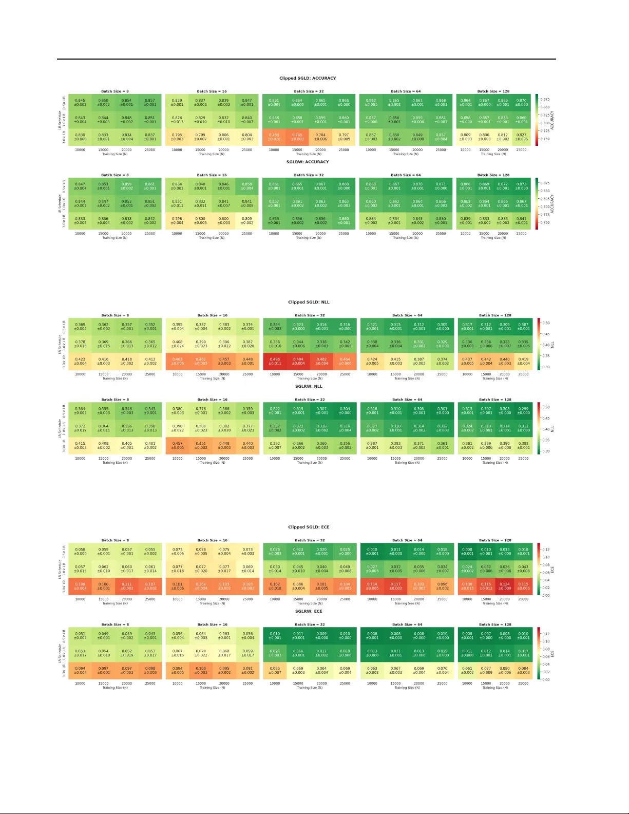
Rob ust Stochastic Gradient Posterior Sampling with Lattice Based Discr etisation Zier Mensch 1 2 Lars Holdijk 3 4 Samuel Duffield 4 Maxwell Aifer 4 Patrick J . Coles 4 Max W elling 5 Miranda Cheng 1 6 7 Abstract Stochastic-gradient MCMC methods enable scal- able Bayesian posterior sampling but often suf- fer from sensitivity to minibatch size and gradi- ent noise. T o address this, we propose Stochas- tic Gradient Lattice Random W alk (SGLR W), an e xtension of the Lattice Random W alk dis- cretization. Unlike con ventional Stochastic Gra- dient Langevin Dynamics (SGLD), SGLR W in- troduces stochastic noise only through the off- diagonal elements of the update co variance; this yields greater robustness to minibatch size while retaining asymptotic correctness. Furthermore, as comparison we analyze a natural analogue of SGLD utilizing gradient clipping. Experimental validation on Bayesian re gression and classifica- tion demonstrates that SGLR W remains stable in regimes where SGLD fails, incl uding in the pres- ence of heavy-tailed gradient noise, and matches or improv es predicti ve performance. 1. Introduction Bayesian methods pro vide a principled framew ork for learn- ing probabilistic models from data and natively capturing uncertainty by replacing the parameter point estimates in frequentist methods with a posterior distribution ov er param- eters. By marginalizing ov er parameters, Bayesian methods act as a form of regularization and enable uncertainty quan- tification and robust model selection ( Neal , 2012 ). In doing so, Bayesian models can potentially mitigate ov erfitting and miscalibration, which are pre valent in modern lar ge-scale, ov erparameterized neural networks ( Guo et al. , 2017 ; Y ang 1 Institute of Physics, Univ ersity of Amsterdam, Netherlands 2 Department of Physics, National T aiwan Univ ersity , T aiwan 3 Department of Computer Science, Uni versity of Oxford, United Kingdom 4 Normal Computing Corporation, New Y ork, Ne w Y ork, USA 5 Amsterdam Machine Learning Lab, Uni versity of Amster - dam, Netherlands 6 Institute for Mathematics, Academia Sinica, T aiwan 7 K orte weg-de Vries Institute for Mathematics, Uni versity of Amsterdam, Netherlands. Correspondence to: Zier Mensch < ziermensch@gmail.com > . Pr eprint. F ebruary 19, 2026. 8 if F igure 1. Comparing SGLD (left) and SGLR W (right) discretisa- tions of Langevin dynamics, we can observe that the lattice based discretisation suppresses large parameter jumps that occur due to minibatch noise, resulting in more stable sampling. et al. , 2023 ). Realizing these benefits in the modern hyper - scaling era, ho we ver , requires posterior inference algorithms that scale to both dataset size and model complexity . W ithin Bayesian methods, Markov chain Monte Carlo (MCMC) ( Neal , 1993 ; Robert et al. , 1999 ) remains the gold standard for posterior sampling, but it is also among the methods most af fected by scalability and computational cost ( Gelman et al. , 1997 ). Alternativ e approaches, including variational inference ( Blei et al. , 2017 ), Laplace approxima- tions ( T ierney & Kadane , 1986 ), and single-pass methods ( Gal & Ghahramani , 2016 ), are often less computationally demanding, but still introduce substantial o verhead in train- ing and inference ( Blei et al. , 2017 ; Lakshminarayanan et al. , 2017 ; W ilson & Izmailo v , 2020 ). As a result, these methods hav e, in some settings, fallen out of f av our relati ve to mod- ern approaches for assessing model trustworthiness, such as explainable and interpretable models ( Li et al. , 2023 ). One core issue of MCMC methods for Bayesian posterior inference is the theoretical requirement to e v aluate the gra- dient of the posterior o ver the entire dataset at each iteration ( W elling & T eh , 2011 ; Ma et al. , 2015 ). W ith gro wing model complexity and dataset size, this is often prohibitiv ely ex- pensiv e. Stochastic-gradient variants of MCMC methods, such as Stochastic Gradient Langevin Dynamics (SGLD) ( W elling & T eh , 2011 ), alle viate this concern to some e xtent by allowing the gradient to be ev aluated on a small mini- batch of data at each iteration. Ho we ver , these methods are still known to be sensiti ve to the minibatch size ( Brosse et al. , 2018 ). As a result, they do not scale to re gimes where 1 Stochastic Gradient Lattice Random W alk only a small minibatch is av ailable at each ev aluation step, or where only a small number of samples from the dataset can be stored in memory , as is becoming increasingly common. In this work, we propose Stochastic Gradient Lattice Ran- dom W alk (SGLR W), a stochastic-gradient extension of the recently introduced Lattice Random W alk (LR W) ( Duffield et al. , 2025 ) discretisation of overdamped Lange vin dynam- ics. LR W replaces the Gaussian increments of Langevin dy- namics with bounded binary or ternary updates on a lattice. As we sho w , unlike SGLD, the stochastic gradient noise in SGLR W enters only through the off-diagonal elements of the cov ariance matrix of the update and therefore remains robust to the minibatch size. This allows SGLR W to sample from the posterior distribution with the same asymptotic correctness as SGLD, but with improv ed stability for small minibatches, as shown in Figure 1 . In short our contributions are as follo ws: • W e propose Stochastic Gradient Lattice Random W alk (SGLR W), a lattice based stochastic-gradient discretisa- tion of ov erdamped Lange vin dynamics (Section 4.2 ). • Extending the analysis of Chen et al. ( 2015 ), we provide a mean-squared-error analysis that justifies its improved stability for small minibatches (Section 4.3 ). • W e validate our theoretical findings on a mix of analyti- cally understood problems and real-world tasks, includ- ing sentiment classification using an LLM (Section 5 ). • W e discuss a clipped version of SGLD as a strong base- line that is analogous to gradient clipping in stochastic gradient descent (Section 5.1 ). 2. Background As stated in the introduction, we consider the problem of minibatch-induced instability in stochastic gradient MCMC methods for Bayesian posterior sampling. Here, we recap the necessary background on Bayesian machine learning, posterior inference, and stochastic gradient methods. Bayesian Machine Learning W e consider the super - vised learning setting where we have observed data D = { ( x i , y i ) } N i =1 and aim to infer a posterior distribution p ( θ | D ) ov er the parameter vector θ ∈ R d . In contrast to frequen- tist approaches, which seek a single point estimate θ ∗ that maximises the likelihood p ( D | θ ) , Bayesian machine learn- ing maintains a full distrib ution ov er parameters, p ( θ | D ) . This posterior distribution captures the uncertainty in our parameter estimates giv en the observed data. The posterior distribution is gi ven by Bayes’ theorem as p ( θ | D ) = p ( D | θ ) p ( θ ) p ( D ) ∝ p ( θ ) N Y i =1 p ( y i | x i , θ ) , (1) where p ( D | θ ) is again the likelihood and p ( θ ) is the prior . Notably , we will often write the posterior distribution as p ( θ | D ) ∝ exp[ − U ( θ )] where U ( θ ) = − log p ( θ ) − N X i =1 log p ( y i | x i , θ ) , (2) is the negati ve log-posterior . Giv en the posterior distribution, predictions for a ne w input x ∗ are then obtained via the posterior predicti ve distribution, p ( y ∗ | x ∗ , D ) = Z p ( y ∗ | x ∗ , θ ) p ( θ | D ) dθ , (3) which marginalises o ver the parameters θ and can thus pro- vide calibrated predictiv e distrib utions. Crucially , howe ver , ev aluating ( 3 ) is generally infeasible, as it in volv es a high- dimensional integral o ver θ . 2.1. Bayesian P osterior Sampling A common approach to Bayesian inference is to replace the integral in ( 3 ) with a Monte Carlo a verage. Most commonly , this is achiev ed by drawing parameter samples θ ∼ p ( θ | D ) from the posterior using a Markov chain Monte Carlo (MCMC) approach. In this work, we specifically focus on MCMC samplers that are expressed as discretisations of stochastic differential equations (SDEs) whose stationary distribution coincides with the tar get posterior ( Ma et al. , 2015 ). Among these, the most common choice is the overdamped Langevin dif fusion, dθ t = f ( θ t ) dt + p 2 D ( θ t ) dW t , (4) where D ( θ t ) is a symmetric positiv e semidefinite dif fusion matrix and f ( θ t ) is the drift. In the conte xt of Bayesian pos- terior sampling, the drift is gi ven by f ( θ t ) = −∇ U ( θ t ) and the diffusion matrix is typically set to D ( θ t ) = I , resulting in the following SDE: dθ t = −∇ U ( θ t ) dt + √ 2 dW t (5) = ( ∇ log p ( θ t ) + N X i =1 ∇ log p ( y i | x i , θ t )) dt + √ 2 dW t . (6) 2 . 1 . 1 . S T O C H A S T I C G R A D I E N T M E T H O D S . As discussed in the introduction, in large-scale settings the requirement to ev aluate the gradient of the posterior over the entire dataset at each iteration is limiting. As such, stochas- tic gradient MCMC (SG-MCMC) methods replace the full posterior gradient with an unbiased minibatch estimator: d ∇ U ( θ ; B ) = −∇ log p ( θ ) − N B X i ∈B ∇ log p ( y i | x i , θ ) , (7) 2 Stochastic Gradient Lattice Random W alk where B ⊂ { 1 , . . . , N } is a minibatch index set of size B , and { ( x i , y i ) } i ∈B ⊂ D are the corresponding datapoints. Stochastic Gradient Langevin Dynamics Stochastic Gradient methods for Bayesian posterior sampling were first introduced by W elling & T eh ( 2011 ) for Langevin dynamics, and only later generalised to other MCMC samplers ( Chen et al. , 2014 ; Ma et al. , 2015 ). Concretely , W elling & T eh ( 2011 ) obtain the follo wing Stochastic Gradient Langevin Dynamics (SGLD) update rule: Definition 2.1 (SGLD Update Rule) . Given a mini- batch B , applying the Euler -Maruyama discretisation to the Langevin SDE Equation ( 5 ) and replacing the full gradient with a minibatch estimate yields the SGLD update: θ t +1 = θ t − δ t d ∇ U ( θ t ; B ) + p 2 δ t ξ t , (8) where ξ t ∼ N (0 , I ) . For the original full-gradient Langevin dynamics, Euler- Maruyama has weak order 1 con v ergence. Howe ver , with stochastic gradients, the con ver gence properties are more subtle ( V ollmer et al. , 2016 ). With a fixed step size δ t = δ , SGLD con verges to a stationary distribution that is biased relativ e to the true posterior, reflecting both discretisation error and the noise from minibatch gradients. T o obtain asymptotically exact expectations, a decreasing step size schedule satisfying δ t → 0 , P t δ t = ∞ , and P t δ 2 t < ∞ needs to be used ( T eh et al. , 2016 ). Howe ver , this does come at the cost of slower mixing as the step size v anishes. In our analysis below , we decompose the stochastic gradient as d ∇ U ( θ ; B ) = ∇ U ( θ ) + ζ ( θ ; B ) and define G ( θ ) to be the minibatch-induced gradient cov ariance, Co v B [ ζ ( θ ; B ) | θ ] = G ( θ ) . Clearly we hav e E B [ ζ ( θ ; B ) | θ ] = 0 . 3. Related W ork W e no w briefly revie w related work on batch-size sensitivity in SG-MCMC methods and large-scale Bayesian inference. Batch-Size Sensitivity . As stated, in practice, SGLD often requires large minibatches for stability , limiting scalability ( Baker et al. , 2019 ). V ariance-reduction and control-v ariate methods reduce noise but introduce memory overhead or require periodic full-data passes ( Dubey et al. , 2016 ; Baker et al. , 2019 ; Li et al. , 2020 ). Alternativ e approaches include adaptiv e subsampling ( Korattikara et al. , 2014 ), precondi- tioning ( Li et al. , 2016 ), and importance sampling ( Li et al. , 2020 ). Moreov er , recent work characterizes stochastic gra- dient noise as hea vy-tailed rather than Gaussian ( Simsekli et al. , 2019 ) and proposes specialized fractional dynamics to retarget the sampling distribution when such noise is present ( Simsekli et al. , 2020 ). While these methods primarily ad- dress the statistical properties of the noise, our solution improv es robustness through its lattice-based discretisation, enabling stable sampling with small minibatches. Large-Scale Bay esian Inference. Bayesian uncertainty estimation is important for large neural models, including large language models, where calibration and robustness are critical ( Y ang et al. , 2023 ). Scalable approximations such as Laplace methods ( Daxberger et al. , 2021 ; Y ang et al. , 2023 ; Chen & Garner , 2024 ; Sliwa et al. , 2025 ) and variational inference ( Harrison et al. , 2024 ; W ang et al. , 2024 ; Xiang et al. , 2025 ; Samplawski et al. , 2025 ) trade accuracy for efficienc y . Recent work shows that sampling-based methods can be applied to large models with appropriate algorithmic structure, as in SGLD-Gibbs ( Kim & Hospedales , 2025 ). 4. Stochastic Gradient Lattice Random W alk W ith the background established in the previous section, we now introduce the proposed method, Stochastic Gra- dient Lattice Random W alk (SGLR W). For this purpose, we first revie w the Lattice Random W alk (LR W) discretisa- tion of Langevin dynamics and then introduce the proposed stochastic gradient extension. 4.1. Lattice Random W alk The Lattice Random W alk (LR W) scheme, recently intro- duced in ( Duf field et al. , 2025 ), proposes an alternati ve to standard SDE discretisations, such as Euler-Maruyama, by substituting Gaussian noise with bounded binary increments. As shown in ( Duf field et al. , 2025 ), this has the benefit of be- ing stable under non-Lipschitz gradients, which are common in deep learning. Additionally , the structure of LR W also lends itself to low-precision, stochastic hardware ( Alaghi & Hayes , 2013 ) and thermodynamic hardware ( Conte et al. , 2019 ) which has recently started to be dev eloped for AI applications ( Melanson et al. , 2025 ). In LR W , at each iteration, the parameters are updated as ∆ θ t +1 = S t , ( S t ) i ∈ {− p 2 δ t , + p 2 δ t } , (9) where each direction ( S t ) i is sampled independently from the following state-dependent probability P h ( S t ) i = ± p 2 δ t    θ t i = 1 2 ± 1 2 q δ t 2 f i ( θ t ) . (10) These probabilities are valid whene ver p δ t / 2 | f i ( θ t ) | ≤ 1 , where we write f i ( θ ) to denote the i th component of the drift vector field f ( θ ) . By construction, the first two conditional moments satisfy E [ S t | θ t ] = δ t f ( θ t ) , E [ S t S ⊤ t | θ t ] = 2 δ t I , (11) 3 Stochastic Gradient Lattice Random W alk and LR W is shown to be weakly first-order consistent with the continuous-time Langevin dynamics in Equation ( 4 ) (Theorem 1 of ( Duffield et al. , 2025 )). With the specific choice of f ( θ ) = −∇ U ( θ ) , LR W thus provides a valid discretisation of the Langevin dynamics in Equation ( 5 ). 4.2. Stochastic Gradient Lattice Random W alk W e now come to the main contrib ution of our work, the proposal of Stochastic Gradient Lattice Random W alk (SGLR W), which replaces the stochastic gradient update rule of SGLD with a lattice-based update: Definition 4.1 (SGLR W Update Rule) . Gi ven a mini- batch B , at the t th iteration, the Stochastic Gradient Lattice Random W alk updates the parameter vector as θ t +1 = θ t + S t . (12) where each coordinate ( S t ) i ∈ {− √ 2 δ t , + √ 2 δ t } is sampled from the state-dependent probability P h ( S t ) i = ± p 2 δ t    θ t i = 1 2 ∓ 1 2 q δ t 2 d ∂ i U ( θ t ; B ) , (13) which is valid whene ver p δ t / 2 | d ∂ i U ( θ t ; B ) | ≤ 1 . W e hypothesize, and analytically ev aluate next, that due to the bounded structure, large fluctuations in stochastic gradients ha ve a less sev ere impact on the update in the case of SGLR W than in the case of SGLD. This is illustrated in Figure 2 , in a one-dimensional multimodal example. Heavy-T ailed Noise Using the stochastic gradient as d ∇ U ( θ ; B ) = ∇ U ( θ ) + ζ ( θ ; B ) , we set U ( θ ) to be the nega- ti ve log-probability of the multimodal Gaussian, and choose ζ ( θ ; B ) to follow a hea vy-tailed α -stable distribution with α < 2 , for which second moments do not exist. This distri- bution was shown to closely resemble the minibatch gradient noise in the standard SGD setting by Simsekli et al. ( 2019 ). F igur e 2. Multimodal univ ariate target with exact gradient cor- rupted by synthetic α -stable noise ( α = 1 . 5 ) of increasing scale. W e observe that as we increase the noise scale SGLD quickly fails while SGLR W remains stable. As Figure 2 sho ws, in this regime, where stability depends critically on whether large stochastic fluctuations can induce rare but catastrophic updates, SGLD fails while SGLR W remains stable. In Appendix A.1 we also provide an analysis using Gaussian gradient noise (Figure 8 ). 4.3. Mean Squared Err or Analysis Having introduced SGLR W , we now present an analysis of the dif ferences between SGLD and SGLR W that highlight the benefits of using SGLR W with small batch sizes. W e follow a similar approach to the analysis of SGLD in Chen et al. ( 2015 ), focussing on the mean squared error (MSE) E ( ˆ ϕ − ¯ ϕ ) 2 between the true posterior expectation ¯ ϕ := Z ϕ ( θ ) p ( θ | D ) dθ . (14) and the ergodic a verage ˆ ϕ := 1 L L X n =1 ϕ ( θ nδ t ) , (15) ov er the discrete-time Mark ov chain { θ nδ t } n ≥ 0 generated by an SG-MCMC method, such as SGLD or SGLR W , with step size δ t . Here, ϕ : R d → R m represents a smooth test function, such as the posterior predictive distribution of a new data point x ∗ , as defined in Equation ( 3 ). As a comparison of the MSE for SGLR W and SGLD, we present the following theorem: Theorem 4.2. Under the Assumption A.1 , we find that the MSE is bounded by the following thr ee contribu- tions MSE ≤ C ( E drift + E disc + E cov ) for some C that depends on the targ et distribution. The covariance err or term for SGLRW is never lar ger than that of SGLD E SGLRW cov ≤ E SGLD cov while the other contributions ar e the same for both. Mor eover , it is strictly smaller whenever 2 ∂ i U ζ i + ζ 2 i is non-vanishing for some dir ection i . The first statement regarding the MSE upper bound, and the precise expression for each of the three contributions, is the content of Theorem A.4 , which is an extension of Theorem 3 of Chen et al. ( 2015 ) to take into account non-vanishing second-order contributions. In particular, the covariance contribution is gi ven by E cov = δ 2 t L L X n =1 E  ∥ M n ∥ 2 F  . (16) 4 Stochastic Gradient Lattice Random W alk F igur e 3. Mean-squared error (MSE) of the posterior cov ariance as a function of the step size δ t , shown for different batch sizes for 50 -dimensional Bayesian linear regression. In the above, the scheme-dependent second-order error M n induced by minibatching is defined as M n ( θ ; B n ) := δ − 2 t E ε n h ∆ θ fb n (∆ θ fb n ) ⊤ − ∆ θ mb n (∆ θ mb n ) ⊤    θ ( n − 1) δ t = θ , B n i , (17) where ∆ θ mb n and ∆ θ fb n denote the one-step increments of the minibatch and full-batch updates, respectiv ely . T o prove the bound in Theorem 4.2 , we observe a lemma quantifying the dif ference between the second-order struc- ture of SGLD and SGLR W Lemma 4.3. The second moment err or of the mini- batch update for SGLR W satisfies M n, SGLR W ( θ ; B n ) = offdiag  M n, SGLD ( θ ; B n )  , (18) wher e M n, SGLD ( θ , B n ) is the second-or der err or for SGLD given by M n, SGLD = ζ ζ ⊤ + ∇ U ζ ⊤ + ζ ∇ U ⊤ . Pr oof. See Appendix A.3 . The above lemma highlights the fact that, in SGLR W , the lattice constraint enforces fixed-magnitude coordinate up- dates, so the diagonal of the one-step second moment of the increment is deterministic. In contrast, for SGLD this diagonal depends on the stochastic gradient and is inflated by minibatch noise. Combining the abov e, we readily obtain the error bound of Theorem 4.2 . This sho ws that under some mild conditions, the SGLR W discretisation achiev es a strictly tighter MSE bound than the SGLD, leading to a more robust implemen- tation of minibatch gradient updates. 4 . 3 . 1 . V A L I DA T I O N A N D P R A C T I C A L C O N S I D E R A T I O N S W e experimentally validate this theoretical finding in Fig- ure 3 , where we compare the MSE for SGLR W and SGLD for Bayesian linear and logistic regression. As δ t increases, SGLD becomes unstable and the cov ariance error explodes, while SGLR W remains stable for all batch sizes. A further discussion of the experimental setup used to generate this insight is provided in Section 5.2 . Despite the theoretical guarantee in Lemma 4.3 , we note that the theoretical restriction p δ t / 2 | d ∂ i U ( θ t ; B ) | ≤ 1 can be challenging to arrange in practice without ov erly conserva- tiv e step size tuning. T o address this, in the implementation we clip the quantity p δ t / 2 | d ∂ i U ( θ t ; B ) | to one, instead of step size tuning. Although this clipping can technically lead to a bias, our empirical ev aluations suggest that this does not pose any serious problem in practice, in the regimes of δ t and minibatch sizes that one is interested in. 5. Experimental ev aluation W e ev aluate SGLR W on posterior sampling problems for linear regression, logistic re gression, and predictive classi- fication tasks. Across all experiments, we vary the mini- batch size B and base step size δ t under matched decaying learning-rate schedules of the form δ t (1 + t ) − 0 . 55 , in line with ( W elling & T eh , 2011 ). All experiments were imple- mented in posteriors ( Duf field et al. , 2024 ). 5.1. Strong Baseline: Clipped SGLD. Similar to our analysis in Section 4.3 , we also compare SGLR W against SGLD in our empirical ev aluation here. Additionally , we introduce Clipped-SGLD as an additional strong baseline. Gradient clipping is standard in large-scale SGD, where saturating the drift pre vents rare large gradients from producing unstable updates. It is therefore natural to ask whether the same stabilisation can be applied to SGLD. W e define the Clipped-SGLD update rule as follows: θ t +1 = θ t − clip( δ t d ∇ U ( θ t ; B ); R ) + p 2 δ t ξ t , (19) where clip( x ; R ) i = sign( x i ) min {| x i | , R } and R = √ 2 δ t . Note that this is a componentwise clipping operation, and deviates slightly from the standard definition of gradient clipping in SGD. In gradient clipping for standard SGD, 5 Stochastic Gradient Lattice Random W alk T able 1. Kullback–Leibler (KL) di ver gence between the true pos- terior and the empirical Gaussian fit of the samples, shown for different samplers (SGLD, SGLR W , Clipped SGLD), minibatch size B , and base learning rate δ t . The Monte Carlo reference KL div ergence, which quantifies the intrinsic sampling v ariability when estimating the analytic posterior, is 0 . 055201 . Bold indicates the lowest KL di vergence for a gi ven ( B , δ t ) pair . Hyperparameters KL Diver gence B δ t SGLD SGLR W Clipped SGLD 8 10 − 3 19.889 6.060 18.184 8 10 − 4 0.483 0.202 0.777 16 10 − 3 7.155 2.317 8.530 16 10 − 4 0.175 0.070 0.204 32 10 − 3 2.441 0.729 3.540 32 10 − 4 0.087 0.064 0.091 64 10 − 3 0.838 0.165 1.114 64 10 − 4 0.063 0.055 0.067 128 10 − 3 0.315 0.074 0.351 128 10 − 4 0.054 0.054 0.061 256 10 − 3 0.140 0.065 0.141 256 10 − 4 0.051 0.056 0.062 512 10 − 3 0.086 0.065 0.088 512 10 − 4 0.052 0.054 0.062 1000 10 − 3 0.058 0.058 0.060 1000 10 − 4 0.052 0.054 0.061 the clipping is performed over the entire update vector ∆ θ t , while here we clip only part of the update v ector . Clipping the entire update vector would result in the SDE ha ving a dif ferent stationary distribution (Appendix A.4 ), while drift-truncated Euler schemes are known to con verge to the exact Lange vin dynamics in the small-step limit ( Roberts & T weedie , 1996 ; Hutzenthaler & Jentzen , 2015 ). In Appendix A.1 we provide the same MSE and heavy-tailed noise analysis for Clipped-SGLD as previously discussed in Section 4.3 for SGLR W . 5.2. Bayesian Linear Regr ession W e first ev aluate SGLR W using a linear–Gaussian model where the posterior admits a closed form. Using the closed- form solution, we can analytically compute the KL div er- gence between the true posterior and the empirical Gaussian fit to the samples. This allows us to provide a more rig- orous e valuation of the empirical performance of SGLR W compared to SGLD and Clipped-SGLD. Concretely , the linear model we consider is giv en by y = X θ + ε, ε ∼ N (0 , σ 2 I ) , (20) where X ∈ R N × d is the design matrix and ε ∈ R N is the noise vector . With a Gaussian prior p ( θ ) = N (0 , τ − 1 I ) , the resulting posterior N ( µ, Σ) is therefore gi ven by Σ − 1 = 1 σ 2 X ⊤ X + τ I , µ = 1 σ 2 Σ X ⊤ y . (21) Or , equivalently , in the negati ve log-posterior form, U ( θ ) = 1 2 σ 2 ∥ y − X θ ∥ 2 + τ 2 ∥ θ ∥ 2 . (22) Setup Synthetic data are generated with N = 1000 and d = 20 , using θ ∗ ∼ N (0 , I ) , σ 2 = 1 . 5 , and τ = 10 − 2 . Each method is run with 2 , 000 parallel particles for 10 , 000 iterations, using matched minibatch sizes and the same de- caying learning-rate schedule. As stated, the performance is quantified using the analytic Kullback–Leibler diver gence between the true posterior N ( µ, Σ) and the empirical Gaussian fit to the samples, com- puted from their estimated mean and cov ariance. 5 . 2 . 1 . R E S U LT S The KL curves reveal two consistent effects, portrayed in T able 1 : (i) step size sensitivity: SGLR W remains stable and continues to decrease KL under larger learning rates δ t where SGLD div erges. (ii) batch efficiency: for comparable KL at matched δ t , SGLR W achie ves the same accuracy with approximately half the minibatch size, indicating greater robustness to stochastic-gradient noise. These trends are accompanied by different empirical cov ari- ance behaviour across methods, as illustrated in Figure 4 . Here we can observe that the error in the diagonal terms of the estimated cov ariance matrices is significantly lower for SGLR W than SGLD and Clipped-SGLD, and in general less impacted by the batch size. F igure 4. Covariance dif ference matrices Σ est − Σ true for Bayesian linear regression at stepsize δ t = 10 − 3 , shown across increas- ing minibatch sizes B . T op: Clipped SGLD. Middle: SGLD. Bottom: SGLR W . Each panel visualizes the deviation of the em- pirical posterior cov ariance from the analytic posterior covariance; the Frobenius norm (Frob) reports the total error magnitude. W e observe that the error in the diagonal terms of the estimated cov ari- ance matrices is lower for SGLR W than SGLD and Clipped-SGLD 6 Stochastic Gradient Lattice Random W alk 5.3. UCI Bayesian Logistic Regr ession W e now compare the sensitivity of SGLR W , SGLD and Clipped-SGLD on a non-Gaussian posterior sampling task, specifically logistic regression with the breast can- cer dataset ( W olberg et al. , 1993 ). The UCI breast cancer dataset consists of 569 samples, 30 features and 2 classes, which results in a 31-dimensional posterior distribution. Setup Since the true posterior is not av ailable analyti- cally , we compare to a gold-standard sample generated with NUTS ( Hoffman et al. , 2014 ) via Pyro ( Bingham et al. , 2019 ). Throughout, we use a standard Gaussian prior on all parameters. In all cases, we ran 5,000 parallel chains for 1,000 steps, retaining only the final sample of each chain. All runs are av eraged ov er 5 seeds. 5 . 3 . 1 . R E S U LT S Comparing the inferred KL div ergence of the three differ - ent methods in T able 2 , we see that SGLR W consistently outperforms SGLD and Clipped-SGLD across learning- rate settings, similar to what was observed in the linear regression experiment. Howe ver , in contrast to the linear regression experiments where Clipped-SGLD performed roughly similarly to SGLD and significantly worse than SGLR W , for the logistic regression experiment considered here Clipped-SGLD sho ws itself as a strong baseline. In the small-batch limit, where we observ e a complete failure of SGLD, Clipped-SGLD performs only slightly worse than SGLR W , and occasionally better as the batch size increases. 5.4. Sentiment Classification With LLM F eatures Having considered two tasks with well-understood posterior distributions, we no w turn to a more realistic problem where in practice issues arise due to the model size impacting the possible size of the minibatch: language modelling using LLMs. Specifically , we ev aluate SGLR W on a sentiment classification task using the IMDB dataset ( Maas et al. , 2011 ), following a setup similar to Harrison et al. ( 2024 ). The dataset consists of 50,000 strongly polarized movie revie ws, split evenly into training and test sets. T o study the effect of data scale, we additionally consider subsampled training sets of varying sizes. Setup For each experiment, we extract fixed sequence embeddings from a pretrained OPT language model ( Zhang et al. , 2022 ) with 350M parameters by taking the final-layer representation of the last token. These embeddings are held fixed, and Bayesian posterior sampling is performed over the parameters of a two-layer binary classification head. This isolates the behaviour of the sampling algorithms from learning the data representation. Each method is run with 15 parallel chains for 10,000 iter - T able 2. Inferred Kullback–Leibler diver gence for the logistic regression problem. The KL diver gence is measured between Gaussian distributions fitted to the empirical mean and covariance of a gold-standard reference sample and those obtained by each algorithm under the specified hyperparameters. Bold indicates the lowest KL di vergence for a gi ven ( B , δ t ) pair . Hyperparameters KL Diver gence B δ t SGLD SGLR W Clipped SGLD 1 10 0 inf 8.3504 9.3560 1 10 − 1 16.6812 6.0144 6.4732 1 10 − 2 10.3472 3.9594 4.2549 2 10 0 inf 7.6706 9.1187 2 10 − 1 8.9809 5.0197 5.5856 2 10 − 2 5.4982 2.6152 2.8710 4 10 0 27.3098 6.9768 8.8915 4 10 − 1 3.7046 3.6632 4.2974 4 10 − 2 3.0155 1.4698 1.6333 8 10 0 19.0951 6.0397 8.4212 8 10 − 1 1.3149 1.9429 2.4981 8 10 − 2 1.9578 1.0051 1.0553 16 10 0 12.0667 4.5631 7.0883 16 10 − 1 0.4993 0.9423 1.2400 16 10 − 2 1.5158 0.8059 0.8027 32 10 0 6.7814 2.8940 4.9928 32 10 − 1 0.2506 0.4538 0.5611 32 10 − 2 1.3235 0.6845 0.6629 64 10 0 3.4559 1.7535 3.0879 64 10 − 1 0.1769 0.2153 0.2417 64 10 − 2 1.2267 0.6490 0.6169 ations, discarding the first 5,000 iterations as burn-in. For each training-set size, we v ary the minibatch size to probe batch-size sensitivity while k eeping learning-rate schedules and other hyperparameters matched across methods. Performance is ev aluated on the held-out test set using clas- sification accuracy , negati ve log-likelihood (NLL), and e x- pected calibration error (ECE). 5 . 4 . 1 . R E S U LT S As highlighted previously , SGLR W has consistently been less sensitiv e to the choice of learning-rate schedule than standard SGLD; it can handle substantially larger step sizes while still maintaining stability across all training-set sizes and minibatch configurations. As such, we first compare the performance of SGLR W against standard SGLD and Clipped-SGLD with small initial step sizes. Follo wing this, we explore the other end of the spectrum, where we compare the performance of SGLR W against Clipped-SGLD at step sizes for which standard SGLD is unstable. Comparison at small step sizes. Fig. 6 shows predicti ve accuracy and negati ve log-likelihood with respect to mini- batch size for a large training-set size ( N = 25 , 000 ) for a run with η 0 = 7 . 5 × 10 − 6 . At small minibatch sizes, SGLD 7 Stochastic Gradient Lattice Random W alk F igur e 5. Relativ e improvement of SGLR W over clipped SGLD at increased learning-rate scale ( η 0 = 1 . 5 × 10 − 4 ). Heatmaps show percentage differences in neg ativ e log-likelihood ( left ) and expected calibration error ( right ) across training-set sizes and minibatch sizes. F igur e 6. Predictive accuracy and ne gati ve log-lik elihood (NLL) as a function of minibatch size for a lar ge training-set size ( N = 25 , 000 ), using base learning schedule with η 0 = 7 . 5 × 10 − 6 . exhibits a de gradation in both accuracy and NLL, whereas SGLR W remains stable across the sweep. As the minibatch size increases, the accuracy of SGLD improv es, while dif- ferences in NLL persist at moderate batch sizes. Similar to SGLR W , Clipped-SGLD also outperforms SGLD in this regime, again highlighting the strength of the baseline. Clipped-SGLD versus SGLR W at larger step sizes. W e next compare Clipped-SGLD and SGLR W in re gimes where standard SGLD is unstable, focusing on step sizes beyond the conservati ve regime. Across all batch sizes considered in Figure 5 , SGLR W consistently outperforms Clipped-SGLD in terms of predicti ve quality , with this beha viour remaining robust across training-set sizes. The relative advantage of SGLR W becomes most pro- nounced in small-to-moderate minibatch regimes. While accuracy dif ferences remain minor , SGLR W consistently at- tains lower negativ e log-likelihood and impro ved calibration relativ e to Clipped-SGLD. A representativ e comparison at an increased learning-rate scale is sho wn in Figure 5 , with complete results across learning-rate schedules reported in Appendix A.5 (Figures 9 , 10 , and 11 ). 6. Conclusion This work introduced Stochastic Gradient Lattice Random W alk (SGLR W), a robust discretisation of Langevin dy- namics for Bayesian inference. By replacing traditional Gaussian increments with coordinate-wise bounded updates, SGLR W significantly reduces sensitivity to minibatch size and stochastic gradient noise, a common failure point for standard SGLD. Our theoretical analysis demonstrated that SGLR W achiev es strictly tighter mean squared error (MSE) bounds than SGLD by confining minibatch-induced noise to the off-diagonal elements of the update co variance. Empirically , SGLR W showed superior stability and predic- ti ve performance across div erse tasks, from linear re gression to LLM-based sentiment classification. This is in compari- son to both standard SGLD as well as a strong baseline in the form of Clipped-SGLD. Notably , it remains stable un- der various conditions where SGLD di v erges and maintains high calibration ev en with small minibatches. Beyond its algorithmic advantages, the structure of SGLR W makes it uniquely suited for implementation on energy- efficient, low-precision, and stochastic hardware ( Duf field et al. , 2025 ), which is becoming increasingly important as the impact of AI on energy consumption and sustainability becomes a major concern ( Aifer et al. , 2025 ). Impact Statement This work introduces a posterior sampling method that is naturally compatible with stochastic hardware and as such SGLR W may reduce energy and memory requirements in practical implementations. Beyond this, this paper presents work whose goal is to adv ance the field of machine learning and as such has many potential societal consequences. 8 Stochastic Gradient Lattice Random W alk References Aifer , M., Belateche, Z., Bramhav ar , S., Camsari, K. Y ., Coles, P . J., Crooks, G., Durian, D. J., Liu, A. J., Marchenkov a, A., Martinez, A. J., et al. Solving the compute crisis with physics-based asics. arXiv preprint arXiv:2507.10463 , 2025. Alaghi, A. and Hayes, J. P . Survey of stochastic comput- ing. ACM T ransactions on Embedded computing systems (TECS) , 12(2s):1–19, 2013. Baker , J., Fearnhead, P ., Fox, E. B., and Nemeth, C. Con- trol variates for stochastic gradient mcmc. Statistics and Computing , 29(3):599–615, 2019. Bingham, E., Chen, J. P ., Janko wiak, M., Obermeyer , F ., Pradhan, N., Karaletsos, T ., Singh, R., Szerlip, P ., Hors- fall, P ., and Goodman, N. D. Pyro: Deep universal prob- abilistic programming. Journal of mac hine learning r e- sear ch , 20(28):1–6, 2019. Blei, D. M., Kucukelbir , A., and McAuliffe, J. D. V aria- tional inference: A revie w for statisticians. J ournal of the American statistical Association , 112(518):859–877, 2017. Brosse, N., Durmus, A., and Moulines, E. The promises and pitfalls of stochastic gradient langevin dynamics. Ad- vances in Neural Information Pr ocessing Systems , 31, 2018. Chen, C., Ding, N., and Carin, L. On the conv ergence of stochastic gradient mcmc algorithms with high-order integrators. Advances in neur al information pr ocessing systems , 28, 2015. Chen, H. and Garner , P . N. Bayesian parameter- efficient fine-tuning for overcoming catastrophic for get- ting. IEEE/ACM T ransactions on Audio, Speech, and Language Pr ocessing , 2024. Chen, T ., Fox, E., and Guestrin, C. Stochastic gradient hamiltonian monte carlo. In International conference on machine learning , pp. 1683–1691. PMLR, 2014. Conte, T ., DeBenedictis, E., Ganesh, N., Hylton, T ., Stra- chan, J. P ., Williams, R. S., Alemi, A., Altenberg, L., Crooks, G., Crutchfield, J., et al. Thermodynamic com- puting. arXiv preprint , 2019. Daxberger , E., Kristiadi, A., Immer , A., Eschenhagen, R., Bauer , M., and Hennig, P . Laplace redux-ef fortless bayesian deep learning. Advances in neural information pr ocessing systems , 34:20089–20103, 2021. Dubey , K. A., J Reddi, S., W illiamson, S. A., Poczos, B., Smola, A. J., and Xing, E. P . V ariance reduction in stochastic gradient langevin dynamics. Advances in neu- ral information pr ocessing systems , 29, 2016. Duffield, S., Donatella, K., Chiu, J., Klett, P ., and Simpson, D. Scalable Bayesian learning with posteriors. arXiv pr eprint arXiv:2406.00104 , 2024. Duffield, S., Aifer, M., Melanson, D., Belateche, Z., and Coles, P . J. Lattice random walk discretisations of stochastic differential equations. arXiv pr eprint arXiv:2508.20883 , 2025. Gal, Y . and Ghahramani, Z. Dropout as a bayesian approx- imation: Representing model uncertainty in deep learn- ing. In international confer ence on machine learning , pp. 1050–1059. PMLR, 2016. Gelman, A., Gilks, W . R., and Roberts, G. O. W eak con- ver gence and optimal scaling of random walk metropolis algorithms. The annals of applied probability , 7(1):110– 120, 1997. Guo, C., Pleiss, G., Sun, Y ., and W einberger , K. Q. On calibration of modern neural networks. In International confer ence on machine learning , pp. 1321–1330. PMLR, 2017. Harrison, J., W illes, J., and Snoek, J. V ariational bayesian last layers. arXiv preprint , 2024. Hoffman, M. D., Gelman, A., et al. The No-U-T urn sampler: adaptiv ely setting path lengths in Hamiltonian Monte Carlo. J. Mach. Learn. Res. , 15(1):1593–1623, 2014. Hutzenthaler , M. and Jentzen, A. Numerical appr oximations of stochastic differ ential equations with non-globally Lip- schitz continuous coefficients , v olume 236. American Mathematical Society , 2015. Kim, M. and Hospedales, T . Lift: Learning to fine-tune via bayesian parameter efficient meta fine-tuning. In The Thirteenth International Confer ence on Learning Repr esentations , 2025. K orattikara, A., Chen, Y ., and W elling, M. Austerity in mcmc land: Cutting the metropolis-hastings budget. In International confer ence on machine learning , pp. 181– 189. PMLR, 2014. Lakshminarayanan, B., Pritzel, A., and Blundell, C. Simple and scalable predictiv e uncertainty estimation using deep ensembles. Advances in neural information pr ocessing systems , 30, 2017. Li, B., Qi, P ., Liu, B., Di, S., Liu, J., Pei, J., Y i, J., and Zhou, B. T rustworthy ai: From principles to practices. ACM Computing Surve ys , 55(9):1–46, 2023. Li, C., Chen, C., Carlson, D., and Carin, L. Preconditioned stochastic gradient langevin dynamics for deep neural networks. In Pr oceedings of the AAAI confer ence on artificial intelligence , v olume 30, 2016. 9 Stochastic Gradient Lattice Random W alk Li, R., W ang, X., Zha, H., and T ao, M. Improving sam- pling accuracy of stochastic gradient mcmc methods via non-uniform subsampling of gradients. arXiv preprint arXiv:2002.08949 , 2020. Ma, Y .-A., Chen, T ., and Fox, E. A complete recipe for stochastic gradient mcmc. Advances in neural informa- tion pr ocessing systems , 28, 2015. Maas, A., Daly , R. E., Pham, P . T ., Huang, D., Ng, A. Y ., and Potts, C. Learning word vectors for sentiment analysis. In Pr oceedings of the 49th annual meeting of the asso- ciation for computational linguistics: Human language technologies , pp. 142–150, 2011. Melanson, D., Abu Khater , M., Aifer , M., Donatella, K., Hunter Gordon, M., Ahle, T ., Crooks, G., Martinez, A. J., Sbahi, F ., and Coles, P . J. Thermodynamic computing system for ai applications. Nature Communications , 16 (1):3757, 2025. Neal, R. M. Probabilistic inference using markov chain monte carlo methods. T echnical report, Department of Computer Science, University of T oronto T oronto, ON, Canada, 1993. Neal, R. M. Bayesian learning for neural networks , volume 118. Springer Science & Business Media, 2012. Robert, C. P ., Casella, G., and Casella, G. Monte Carlo statistical methods , volume 2. Springer , 1999. Roberts, G. O. and T weedie, R. L. Exponential con vergence of langevin distributions and their discrete approxima- tions. Bernoulli , 2(4):341–363, 1996. Samplawski, C., Cobb, A. D., Acharya, M., Kaur , R., and Jha, S. Scalable bayesian low-rank adaptation of large language models via stochastic variational subspace in- ference. arXiv preprint , 2025. Simsekli, U., Sagun, L., and Gurbuzbalaban, M. A tail-index analysis of stochastic gradient noise in deep neural net- works. In International Confer ence on Machine Learning , pp. 5827–5837. PMLR, 2019. Simsekli, U., Zhu, L., T eh, Y . W ., and Gurbuzbalaban, M. Fractional underdamped Lange vin dynamics: Retargeting SGD with momentum under hea vy-tailed gradient noise. In International Confer ence on Machine Learning , pp. 8970–8980. PMLR, 2020. Sliwa, J., Schneider , F ., Hennig, P ., and Hern ´ andez-Lobato, J. M. Mitigating for getting in lo w rank adaptation. In Sec- ond W orkshop on T est-T ime Adaptation: Putting Updates to the T est! at ICML 2025 , 2025. T eh, Y . W ., Thiery , A. H., and V ollmer , S. J. Consistency and fluctuations for stochastic gradient lange vin dynamics. The J ournal of Machine Learning Researc h , 17(1):193– 225, 2016. T ierney , L. and Kadane, J. B. Accurate approximations for posterior moments and marginal densities. Journal of the american statistical association , 81(393):82–86, 1986. V ollmer , S. J., Zygalakis, K. C., and T eh, Y . W . Exploration of the (non-) asymptotic bias and v ariance of stochastic gradient lange vin dynamics. Journal of Mac hine Learn- ing Resear ch , 17(159):1–48, 2016. W ang, Y ., Shi, H., Han, L., Metaxas, D., and W ang, H. Blob: Bayesian low-rank adaptation by backpropagation for large language models. Advances in Neural Information Pr ocessing Systems , 37:67758–67794, 2024. W elling, M. and T eh, Y . W . Bayesian learning via stochastic gradient lange vin dynamics. In Pr oceedings of the 28th international conference on mac hine learning (ICML-11) , pp. 681–688, 2011. W ilson, A. G. and Izmailov , P . Bayesian deep learning and a probabilistic perspectiv e of generalization. Advances in neural information pr ocessing systems , 33:4697–4708, 2020. W olberg, W ., Mangasarian, O., Street, N., and Street, W . Breast Cancer W isconsin (Diagnostic). UCI Machine Learning Repository , 1993. DOI: https://doi.org/10.24432/C5D W2B. Xiang, H., Xu, J., and Lu, Q. Fine-tuning llms with varia- tional bayesian last layer for high-dimensional bayesian optimzation. arXiv preprint , 2025. Y ang, A. X., Robeyns, M., W ang, X., and Aitchison, L. Bayesian low-rank adaptation for lar ge language models. arXiv pr eprint arXiv:2308.13111 , 2023. Zhang, S., Roller , S., Goyal, N., Artetxe, M., Chen, M., Chen, S., Dewan, C., Diab, M., Li, X., Lin, X. V ., et al. Opt: Open pre-trained transformer language models. arXiv pr eprint arXiv:2205.01068 , 2022. 10 Stochastic Gradient Lattice Random W alk A. A ppendix A.1. Analysis plots including Clipped SGLD For completeness, we also include Clipped SGLD in the plots for the analysis. For the cov ariance MSE analysis (Figure 3 ), Clipped SGLD already mitigates the sharp error explosion observed for SGLD at larger stepsizes (Figure 7 ). Howe ver , across batch sizes and learning rates, SGLR W consistently attains comparable or lower co variance MSE throughout the stable regime. For the hea vy-tailed noise rob ustness analysis (Figure 2 ), both Clipped SGLD and SGLR W prevent the se vere instability exhibited by SGLD under heavy-tailed gradient noise. Across noise scales, SGLR W maintains a closer qualitativ e agreement with the target distrib ution than Clipped SGLD. A.2. Proof of Theor em 4.2 In this appendix we prov e Theorem 4.2 . The argument follo ws the Poisson-equation frame work of ( Chen et al. , 2015 ); we restate the required notation so the appendix is self-contained. F igur e 7. Mean-squared error (MSE) of the posterior cov ariance as a function of the stepsize δ t , sho wn for dif ferent batch sizes. T op: 50 -dimensional Bayesian linear regression. Bottom: Bayesian logistic regression on the breast cancer dataset ( W olberg et al. , 1993 ). F igure 8. Multimodal univ ariate target with exact gradient corrupted by synthetic noise of increasing scale. Left: Gaussian noise ( α = 2 ). Right: heavy-tailed noise dra wn from an α -stable distribution with α = 1 . 5 . 11 Stochastic Gradient Lattice Random W alk Generator and Kolmogor ov operators. Consider a continuous-time It ˆ o diffusion on R d with infinitesimal generator L g ( θ ) = f ( θ ) · ∇ g ( θ ) + D ( θ ) : ∇ 2 g ( θ ) , (23) with f the drift of the SDE in ( 4 ) . Let ( e t L ) t ≥ 0 denote the associated K olmogorov (backward) semigroup, so that for an y suitable test function g , E [ g ( θ t ) | θ 0 = θ ] = ( e t L g )( θ ) . (24) Since e t L is generally intractable, we consider a time- δ t numerical update with one-step Marko v operator P ( L ) δ t defined by E [ g ( θ nδ t ) | θ ( n − 1) δ t ] = ( P ( L ) δ t g )( θ ( n − 1) δ t ) . (25) A one-step scheme P δ t is a weak order- K local integrator if, for all sufficiently smooth g , we have ( P δ t g )( θ ) = ( e δ t L g )( θ ) + O ( δ K +1 t ) . (26) Stochastic gradients and random one-step operators. The Euler-Maruyama discretization scheme is kno wn to be weak order-one. W e now e xamine the effect of using minibatches. In SGLD as well as SGLR W , the exact drift f is replaced by a minibatch approximation b f . Let e P ( n ) δ t denote the resulting (random) one-step Markov operator at iteration n , i.e. E [ g ( θ nδ t ) | θ ( n − 1) δ t ] = ( e P ( n ) δ t g )( θ ( n − 1) δ t ) . (27) For a gi ven minibatch B , define ζ ( θ ; B ) := f ( θ ) − b f ( θ ; B ) . (28) and the associated first-order differential operator (∆ V n g )( θ ; B ) := ζ ( θ ; B n ) · ∇ g ( θ ) . (29) capturing the error due to the minibatch drift error . Note that for overdamped Langevin diffusion, we hav e f = −∇ U , b f ( θ ; B ) = − d ∇ U ( θ ; B ) , so that ζ ( θ ; B ) = d ∇ U ( θ ; B ) − ∇ U ( θ ) . Beyond the first-order drift perturbation, minibatching can induce a second-order correction through the conditional second moment of the increment. W e define the second-order differential operator (∆ A n g )( θ ) := 1 2 M n ( θ ) : ∇ 2 g ( θ ) , (30) with M n ( θ , B n ) := δ − 2 t E ξ n  ∆ θ fb n (∆ θ fb n ) ⊤ − ∆ θ mb n (∆ θ mb n ) ⊤   θ ( n − 1) δ t = θ , B n  . (31) Here ∆ θ mb n and ∆ θ fb n denote the one-step increments of the minibatch and full-batch updates, respectiv ely , and E ξ n [ · ] denotes expectation with respect to the internal randomness of the update at step n (e.g. injected Gaussian noise or lattice path sampling). Poisson equation. Giv en a smooth observ able ϕ : R d → R , define its stationary e xpectation under the in variant distribution π by ¯ ϕ := Z ϕ ( θ ) π ( θ ) dθ . (32) W e analyze ergodic av erages via the Poisson equation L ψ = ϕ − ¯ ϕ, (33) and express finite-time errors in terms of the corresponding solution ψ . W e assume that, for the Poisson solution ψ , the remainder satisfies the L yapunov-weighted bound, in the sense that there exists a constant p 0 > 0 such that |R n ψ ( θ ) | ≤ C V ( θ ) p 0 , uniformly in n and δ t ∈ (0 , 1] . (34) L yapunov-Poisson r egularity . 12 Stochastic Gradient Lattice Random W alk Assumption A.1. Let ψ solve the Poisson equation L ψ = ϕ − ¯ ϕ . Assume there exists a function V : R d → [1 , ∞ ) such that: (i) ( Derivative control ) There e xist constants C k , p k > 0 for k = 0 , 1 , 2 , 3 , 4 such that ∥ D k ψ ( θ ) ∥ ≤ C k V ( θ ) p k . (35) (ii) ( Uniform moments along the chain ) There exist constants p ∗ such that for all p ≤ p ∗ , sup n E [ V ( θ nδ t ) p ] < ∞ . (36) (iii) ( Growth compatibility ) F or the constant p ∗ and some C > 0 , for all p ≤ p ∗ and all s ∈ (0 , 1) , V p ( sθ + (1 − s ) ϑ ) ≤ C  V p ( θ ) + V p ( ϑ )  . (37) (iv) ( Uniform second-moment bound ) The second-order coefficient field satisfies sup n E  ∥ M n ( θ ( n − 1) δ t ) ∥ 2 F  < ∞ . (38) (v) ( Increment moment contr ol ) There exist constants C > 0 and exponents q 2 , q 4 > 0 such that, for all n , E ξ n , B n  ∥ ∆ θ n ∥ 2 k   θ ( n − 1) δ t  ≤ C δ k t V ( θ ( n − 1) δ t ) q 2 k , k ∈ { 1 , 2 } , (39) where ∆ θ n := θ nδ t − θ ( n − 1) δ t . (vi) ( Third-moment tensor contr ol ) There exist constants C > 0 and an exponent q 3 > 0 such that, for all n ,    E ξ n , B n  (∆ θ mb n ) ⊗ 3   θ ( n − 1) δ t  − E ξ n  (∆ θ fb n ) ⊗ 3   θ ( n − 1) δ t     ≤ C δ 2 t V ( θ ( n − 1) δ t ) q 3 . (40) (vii) ( Unbiased minibatch estimator ) The minibatch drift estimator is conditionally unbiased, in the sense that E B n  ζ ( θ ( n − 1) δ t ; B n )   θ ( n − 1) δ t  = 0 a.s. for all n, (41) where ζ ( θ ; B ) := f ( θ ) − b f ( θ ; B ) denotes the minibatch drift error . Note that the deri vati ve bounds ( 35 ) in Assumption A.1 can be verified by constructing a L yapuno v function V : R d → [1 , ∞ ) which tends to infinity as θ → ∞ , is twice continuously dif ferentiable with bounded second deri v ativ es, and satisfies the following conditions, as sho wn in the Appendix C of ( Chen et al. , 2015 ): (a) ( Lyapunov drift condition ) There e xist constants α, β > 0 such that the exact drift field f satisfies ⟨∇V ( θ ) , f ( θ ) ⟩ ≤ − α V ( θ ) + β . (42) (b) ( Minibatch-induced drift fluctuations ) There exists p H ≥ 2 such that E ξ n , B n  ∥ ζ ( θ ( n − 1) δ t ; B n ) ∥ 2   θ ( n − 1) δ t = θ  ≤ C V ( θ ) p H , (43) together with the growth condition ∥∇V ( θ ) ∥ 2 + ∥ f ( θ ) ∥ 2 ≤ C V ( θ ) . (44) Remark A.2 . Throughout, we write θ ( n − 1) δ t = θ and recall that for overdamped Lange vin diffusion we hav e ζ ( θ ; B ) = d ∇ U ( θ ; B ) − ∇ U ( θ ) . Assumptions A.1 (v)–(vi) hold for SGLD and SGLR W for varying requirements on the minibatch noise ζ . 13 Stochastic Gradient Lattice Random W alk 1. SGLD. • Second moment ( k = 1 ): From ∆ θ mb n = − δ t ( ∇ U ( θ ) + ζ ) + √ 2 δ t ξ n , and using ∥ a + b ∥ 2 ≤ 2 ∥ a ∥ 2 + 2 ∥ b ∥ 2 we hav e E ξ n , B n  ∥ ∆ θ mb n ∥ 2 | θ  ≤ 2 δ 2 t E B n  ∥∇ U ( θ ) + ζ ∥ 2 | θ  + 4 d δ t . (45) Thus, assuming E B n  ∥ ζ ∥ 2 | θ  ≤ C V ( θ ) q 2 , ∥∇ U ( θ ) ∥ 2 ≤ C V ( θ ) , (46) yields E B n ,ε n  ∥ ∆ θ mb n ∥ 2 | θ  = O ( δ t ) . (47) • F ourth moment contr ol ( k = 2 ): Similarly , E ξ n , B n  ∥ ∆ θ mb n ∥ 4 | θ  ≤ C δ 4 t E B n  ∥∇ U ( θ ) + ζ ∥ 4 | θ  + C δ 2 t . (48) Hence, if E B n  ∥ ζ ∥ 4 | θ  ≤ C V ( θ ) q 4 , (49) then E ξ n , B n  ∥ ∆ θ mb n ∥ 4 | θ  = O ( δ 2 t ) . (50) • Thir d-moment contr ol: From the expansion in ( 99 ) , the difference in ( 40 ) arises from cubic drift noise interaction terms, and scales as O ( δ 3 t ) . Assuming E B n  ∥ ζ ∥ 3 | θ  ≤ C V ( θ ) q 3 , (51) this difference is bounded by C δ 2 t V ( θ ) q 3 for δ t ∈ (0 , 1] . 2. SGLRW . • Incr ement contr ol ( k = 1 , 2 ): As ∥ ∆ θ mb n ∥ 2 = 2 d δ t and ∥ ∆ θ mb n ∥ 4 = 4 d 2 δ 2 t , the bound ( 39 ) holds without any assumption on ζ . • Thir d-moment contr ol: As shown in ( 113 ) , the third-order conditional moments are batch-independent when at least two of the three directions coincide. For distinct indices ( i, j, k ) , the dif ference is O ( δ 3 t ) . Consequently , ( 40 ) holds provided E B n  ∥ ζ ∥ 3 | θ  ≤ C V ( θ ) q 3 . (52) In SGLD as well as SGLR W , the exact drift f is replaced by a minibatch approximation b f . Since the underlying Euler- Maruyama scheme is a weak order-one integrator , we can deriv e a refined weak expansion for the resulting random operator , explicitly capturing the drift and co v ariance perturbations. Lemma A.3 (Refined weak expansion) . Consider a numerical integr ator that is weak order -one for the full batch dynamics. Let e P ( n ) δ t denote the random operator obtained by r eplacing the exact drift with a mini-batch estimator , for which Assumption A.1 holds. Then e P ( n ) δ t admits the expansion: e P ( n ) δ t ψ ( θ ) = ψ ( θ ) + δ t ( L − ∆ V n ) ψ ( θ ) − δ 2 t ∆ A n ψ ( θ ) + δ 2 t R n ψ ( θ ) , (53) wher e ∆ V n is the first-or der drift perturbation, ∆ A n is the second-or der covariance perturbation, and |R n ψ ( θ ) | ≤ C V ( θ ) p 0 uniformly in n and δ t ∈ (0 , 1] . 14 Stochastic Gradient Lattice Random W alk Pr oof. By T aylor’ s theorem with integral remainder applied to the minibatch increment, ψ ( θ + ∆ θ mb n ) = ψ ( θ ) + ∇ ψ ( θ ) · ∆ θ mb n + 1 2 ∆ θ mb n (∆ θ mb n ) ⊤ : ∇ 2 ψ ( θ ) + 1 6 ∇ 3 ψ ( θ ) : (∆ θ mb n ) ⊗ 3 + R 4 ( θ , ∆ θ mb n ) , (54) where R 4 ( θ , ∆ θ ) = 1 6 Z 1 0 (1 − s ) 3 ∇ 4 ψ ( θ + s ∆ θ ) : ∆ θ ⊗ 4 ds. (55) For a gi ven minibatch B n , taking the conditional expectation yields e P ( n ) δ t ψ ( θ ) = ψ ( θ ) + ∇ ψ ( θ ) · E ξ n [∆ θ mb n | θ ] + 1 2 E ξ n [∆ θ mb n (∆ θ mb n ) ⊤ | θ ] : ∇ 2 ψ ( θ ) + 1 6 ∇ 3 ψ ( θ ) : E ξ n [(∆ θ mb n ) ⊗ 3 | θ ] + E ξ n [ R 4 ( θ , ∆ θ mb n ) | θ ] . (56) By definition of the increment-based drift difference, ζ ( θ ; B n ) = f ( θ ) − b f ( θ ; B ) , (57) so ∇ ψ ( θ ) · E ξ n [∆ θ mb n | θ ] = δ t ∇ ψ ( θ ) · b f ( θ ; B ) = δ t f ( θ ) · ∇ ψ ( θ ) − δ t ∆ V n ψ ( θ ) . (58) Similarly , by definition of ∆ A n , 1 2 E ξ n [∆ θ mb n (∆ θ mb n ) ⊤ | θ ] : ∇ 2 ψ ( θ ) = 1 2 E ξ n [∆ θ fb n (∆ θ fb n ) ⊤ | θ ] : ∇ 2 ψ ( θ ) − δ 2 t ∆ A n ψ ( θ ) . (59) W e now treat the cubic term by adding and subtracting the full-batch third moment: 1 6 ∇ 3 ψ ( θ ) : E ξ n [(∆ θ mb n ) ⊗ 3 | θ ] = 1 6 ∇ 3 ψ ( θ ) : E ξ n [(∆ θ fb n ) ⊗ 3 | θ ] + 1 6 ∇ 3 ψ ( θ ) :  E ξ n [(∆ θ mb n ) ⊗ 3 | θ ] − E ξ n [(∆ θ fb n ) ⊗ 3 | θ ]  . (60) Since the full-batch scheme is weak order one, its contribution is absorbed into the O ( δ 2 t ) remainder of the full-batch expansion. By Assumption A.1 (vi), the difference of third-order moments is O ( δ 2 t V ( θ ) q 3 ) , so the net cubic contribution is O ( δ 2 t V ( θ ) p 0 ) . For the fourth-order remainder , using | T : x ⊗ 4 | ≤ ∥ T ∥ ∥ x ∥ 4 and Assumption A.1 (i) with k = 4 , we obtain | R 4 ( θ , ∆ θ mb n ) | ≤ C ∥ ∆ θ mb n ∥ 4 Z 1 0 V ( θ + s ∆ θ mb n ) p 4 ds. (61) By Assumption A.1 (iii), V ( θ + s ∆ θ mb n ) p 4 ≤ C ( V ( θ ) p 4 + V ( θ + ∆ θ mb n ) p 4 ) for s ∈ (0 , 1) . T aking conditional expec- tation, applying the increment fourth-moment bound in Assumption A.1 (v), and using the uniform moment bound in Assumption A.1 (ii), yields E ξ n [ | R 4 ( θ , ∆ θ mb n ) | | θ , B n ] ≤ C δ 2 t V ( θ ) p 0 , (62) uniformly in n and δ t ∈ (0 , 1] . Collecting all O ( δ 2 t ) contributions into R n yields the stated expansion. 15 Stochastic Gradient Lattice Random W alk Theorem A.4. Under the Assumption A.1 , ther e exists C > 0 , independent of ( L, δ t ) , such that E ( ˆ ϕ − ¯ ϕ ) 2 ≤ C 1 L 2 L X n =1 E  ∥ ζ n ∥ 2  + 1 Lδ t + 1 L 2 δ 2 t + δ 2 t + δ 2 t L L X n =1 E  ∥ M n ∥ 2  ! . (63) Pr oof. First write ˆ ϕ − ¯ ϕ = 1 L P L n =1 L ψ ( θ nδ t ) . Ne xt, use Lemma A.3 to rewrite L ψ ( θ ) , and using E ξ n [ ψ ( θ nδ t ) | θ ( n − 1) δ t , B n ] = ( e P ( n ) δ t ψ )( θ ( n − 1) δ t ) , we obtain ˆ ϕ − ¯ ϕ = 1 Lδ t  ψ ( θ Lδ t ) − ψ ( θ δ t )  − 1 Lδ t L X n =1  E ξ n [ ψ ( θ nδ t ) | θ ( n − 1) δ t ] − ψ ( θ nδ t )  + 1 L L X n =1 ∆ V n ψ ( θ ( n − 1) δ t ) + δ t L L X n =1 ∆ A n ψ ( θ ( n − 1) δ t ) − δ t L L X n =1 R n ψ ( θ ( n − 1) δ t ) . (64) T aking squares and using ( a + b + c + d + e ) 2 ≤ 5( a 2 + b 2 + c 2 + d 2 + e 2 ) gi ves E ( ˆ ϕ − ¯ ϕ ) 2 ≤ C ( α 1 + α 2 + α 3 + α 4 + α 5 ) , (65) where α 1 := E "  ψ ( θ Lδ t ) − ψ ( θ δ t ) Lδ t  2 # , (66) α 2 := E   1 L 2 δ 2 t L X n =1  E ξ n [ ψ ( θ nδ t ) | θ ( n − 1) δ t ] − ψ ( θ nδ t )  ! 2   , (67) α 3 := E   1 L 2 L X n =1 ∆ V n ψ ( θ ( n − 1) δ t ) ! 2   , (68) α 4 := E   δ t L L X n =1 ∆ A n ψ ( θ ( n − 1) δ t ) ! 2   , (69) α 5 := E   δ t L L X n =1 R n ψ ( θ ( n − 1) δ t ) ! 2   . (70) (i) α 1 . By L yapunov control of ψ (Assumption A.1 (i–ii) with k = 0 ), sup n E [ ψ ( θ nδ t ) 2 ] < ∞ , hence α 1 ≤ C L 2 δ 2 t . (71) (ii) α 2 . Let Z n := E ξ n [ ψ ( θ nδ t ) | θ ( n − 1) δ t ] − ψ ( θ nδ t ) , (72) so that { Z n } n ≥ 1 is a martingale dif ference sequence and hence α 2 = 1 L 2 δ 2 t L X n =1 E  V ar( ψ ( θ nδ t ) | θ ( n − 1) δ t )  . (73) Write θ := θ ( n − 1) δ t and ∆ θ n := θ nδ t − θ . By the fundamental theorem of calculus, ψ ( θ + ∆ θ n ) − ψ ( θ ) = ∆ θ n · Z 1 0 ∇ ψ ( θ + s ∆ θ n ) ds. (74) 16 Stochastic Gradient Lattice Random W alk Therefore, V ar( ψ ( θ nδ t ) | θ ) = V ar( ψ ( θ nδ t ) − ψ ( θ ) | θ ) ≤ E  ( ψ ( θ + ∆ θ n ) − ψ ( θ )) 2 | θ  ≤ E  ∥ ∆ θ n ∥ 2 Z 1 0 ∥∇ ψ ( θ + s ∆ θ n ) ∥ 2 ds     θ  , (75) where we used Cauchy-Schwarz. By Assumption A.1 (i), ∥∇ ψ ( x ) ∥ 2 ≤ C V ( x ) 2 p 1 , and by Assumption A.1 (iii), V ( θ + s ∆ θ n ) 2 p 1 ≤ C  V ( θ ) 2 p 1 + V ( θ + ∆ θ n ) 2 p 1  , s ∈ (0 , 1) . (76) Hence, V ar( ψ ( θ nδ t ) | θ ) ≤ C E h ∥ ∆ θ n ∥ 2  V ( θ ) 2 p 1 + V ( θ nδ t ) 2 p 1  | θ i . (77) T aking conditional expectation with respect to B n and using the tower property yields E [V ar( ψ ( θ nδ t ) | θ ) | θ ] ≤ C E h ∥ ∆ θ n ∥ 2  V ( θ ) 2 p 1 + V ( θ nδ t ) 2 p 1  | θ i . (78) By Assumption A.1 (v), the increment satisfies the conditional second-moment bound E  ∥ ∆ θ n ∥ 2 | θ ( n − 1) δ t  ≤ C δ t V ( θ ( n − 1) δ t ) q , (79) for some q > 0 . T aking total expectations and using Assumption A.1 (ii) to control moments of V ( θ nδ t ) yields E  V ar( ψ ( θ nδ t ) | θ ( n − 1) δ t , B n )  ≤ C δ t . (80) Substituting this bound into the definition of α 2 giv es α 2 ≤ 1 L 2 δ 2 t L X n =1 C δ t = C Lδ t . (81) (iii) α 3 . Set X n := ∆ V n ψ ( θ ( n − 1) δ t ) . By the assumed unbiasedness we have E [ X n | θ ( n − 1) δ t ] = 0 , so { X n } is a martingale dif ference sequence and therefore cross-terms v anish: E h L X n =1 X n  2 i = L X n =1 E [ X 2 n ] . (82) Moreov er , | X n | = | ζ ( θ ( n − 1) δ t ; B n ) · ∇ ψ ( θ ( n − 1) δ t ) | ≤ ∥ ζ ( θ ( n − 1) δ t ; B n ) ∥ ∥∇ ψ ( θ ( n − 1) δ t ) ∥ , (83) so by Assumption A.1 (i-ii), E [ X 2 n ] ≤ C E  ∥ ζ ( θ ( n − 1) δ t ; B n ) ∥ 2  , (84) absorbing ∥∇ ψ ∥ 2 into the constant using the L yapunov moment bounds. Hence α 3 = 1 L 2 L X n =1 E [ X 2 n ] ≤ C L 2 L X n =1 E  ∥ ζ ( θ ( n − 1) δ t ; B n ) ∥ 2  . (85) (iv) α 4 . By Cauchy-Schwarz, α 4 ≤ δ 2 t L L X n =1 E  (∆ A n ψ ( θ ( n − 1) δ t )) 2  . (86) 17 Stochastic Gradient Lattice Random W alk Using ∆ A n f = 1 2 M n : ∇ 2 f and the Hilbert-Schmidt inequality , | ∆ A n ψ ( θ ) | ≤ 1 2 ∥ M n ( θ ) ∥ F ∥∇ 2 ψ ( θ ) ∥ F ≤ C ∥ M n ( θ ) ∥ V ( θ ) p 2 , (87) where we used Assumption A.1 (i) with k = 2 . T aking expectations and using Assumptions A.1 (ii, iv), we obtain E  (∆ A n ψ ( θ ( n − 1) δ t )) 2  ≤ C E  ∥ M n ( θ ( n − 1) δ t ; B n ) ∥ 2  . (88) Therefore α 4 ≤ C δ 2 t L L X n =1 E  ∥ M n ( θ ( n − 1) δ t ; B n ) ∥ 2  . (89) (v) α 5 . By Cauchy-Schwarz and the remainder bound from Lemma A.3 , α 5 ≤ δ 2 t L L X n =1 E  ( R n ψ ( θ ( n − 1) δ t )) 2  ≤ C δ 2 t L L X n =1 E  V ( θ ( n − 1) δ t ) 2 p 0  ≤ C δ 2 t , (90) using Assumption A.1 (ii). Combining the bounds on α 1 , . . . , α 5 yields ( 63 ). A.3. Conditional Covariance and Moments of SGLD and SGLR W Updates W e decompose the stochastic gradient as d ∇ U ( θ ; B ) = ∇ U ( θ ) + ζ ( θ ; B ) , E B [ ζ ( θ ; B ) | θ ] = 0 , Co v B [ ζ ( θ ; B ) | θ ] = G ( θ ) , (91) where G ( θ ) quantifies the minibatch-induced gradient cov ariance. Recall the definition the second-order minibatch contribution M n used in Theorem A.4 : M n ( θ , B n ) := δ − 2 t E ξ n  ∆ θ mb n (∆ θ mb n ) ⊤ − ∆ θ fb n (∆ θ fb n ) ⊤   θ ( n − 1) δ t = θ , B n  , (92) where ε n denotes the internal randomness of the integrator . SGLD. The standard SGLD update is ∆ θ t = − δ t ( ∇ U ( θ t ) + ζ t ) + √ 2 δ t ξ t with ξ t ∼ N (0 , I ) . Using the independence of ξ t and ζ t , and E [ ζ t | θ t ] = 0 , the first and second moments are: E [∆ θ t | θ t ] = − δ t ∇ U ( θ t ) , (93) E [∆ θ t ∆ θ ⊤ t | θ t ] = 2 δ t I + δ 2 t  ∇ U ( θ t ) ∇ U ( θ t ) ⊤ + G ( θ t )  . (94) W e next deri ve the second-order minibatch contrib ution M n . Fix θ and a minibatch B , define the full-batch and minibatch increments (sharing the same Gaussian ξ ) ∆ θ fb = − δ t ∇ U ( θ ) + p 2 δ t ξ , ∆ θ mb = − δ t ( ∇ U ( θ ) + ζ ) + p 2 δ t ξ = ∆ θ fb − δ t ζ . (95) Expanding the outer products giv es ∆ θ mb ∆ θ mb ⊤ − ∆ θ fb ∆ θ fb ⊤ = − δ t ∆ θ fb ζ ⊤ − δ t ζ (∆ θ fb ) ⊤ + δ 2 t ζ ζ ⊤ . (96) T aking conditional expectation ov er the internal randomness ξ and using E ξ [∆ θ fb | θ ] = − δ t ∇ U ( θ ) yields E ξ  ∆ θ mb ∆ θ mb ⊤ − ∆ θ fb ∆ θ fb ⊤   θ , B  = δ 2 t  ζ ζ ⊤ + ∇ U ( θ ) ζ ⊤ + ζ ∇ U ( θ ) ⊤  . (97) 18 Stochastic Gradient Lattice Random W alk Therefore, with M n defined as in ( 30 ), M n, SGLD ( θ ; B ) = ζ ( θ ; B ) ζ ( θ ; B ) ⊤ + ∇ U ( θ ) ζ ( θ ; B ) ⊤ + ζ ( θ ; B ) ∇ U ( θ ) ⊤ . (98) A veraging additionally ov er minibatches giv es E B [ M n, SGLD ( θ , B ) | θ ] = G ( θ ) . For the third moment, let u t = − δ t ( ∇ U + ζ t ) and w t = √ 2 δ t ξ t . Expanding E [( u t + w t ) ⊗ 3 | θ t ] , terms with odd po wers of ξ t vanish. The remaining terms are E [ u ⊗ 3 t ] and the cross-terms E [ u t ⊗ w t ⊗ w t ] (and permutations). The leading O ( δ 2 t ) error comes from the cross-terms: E [ u t,i w t,j w t,k | θ t ] = E [ − δ t ( ∂ i U + ζ i ) · 2 δ t δ j k ] = − 2 δ 2 t ∂ i U δ j k . Because E [ ζ i ] = 0 , the O ( δ 2 t ) part of the tensor is identical for full-batch and minibatch schemes. The third-order moments of the noise appear in the E [ u ⊗ 3 t ] expansion. By expanding the cubic terms and using E [ ζ t ] = 0 , the tensor entries decompose as follows: E [∆ θ i ∆ θ j ∆ θ k | θ t ] =            − 6 δ 2 t ∂ i U − δ 3 t  ( ∂ i U ) 3 + 3 ∂ i U G ii + E [ ζ 3 i | θ t ]  , i = j = k , − 2 δ 2 t ∂ k U − δ 3 t  ( ∂ i U ) 2 ∂ k U + ∂ k U G ii + 2 ∂ i U G ik + E [ ζ 2 i ζ k | θ t ]  , i = j  = k , − δ 3 t  ∂ i U ∂ j U ∂ k U + P cyc ( i,j,k ) ∂ i U G j k + E [ ζ i ζ j ζ k | θ t ]  , i, j, k all distinct , (99) and permutations. SGLR W . For the lattice random walk (LR W) discretisation, each coordinate i takes a binary step ∆ θ t,i ∈ {± √ 2 δ t } with probabilities P h ∆ θ t,i = p 2 δ t    θ t , ζ t i = 1 2 − 1 2 q δ t 2 [ ∂ i U ( θ t ) + ζ t,i ] , (100) P h ∆ θ t,i = − p 2 δ t    θ t , ζ t i = 1 2 + 1 2 q δ t 2 [ ∂ i U ( θ t ) + ζ t,i ] . (101) Conditionally on ( θ t , ζ t ) the coordinates are independent. A short calculation gi ves E [∆ θ t | θ t , ζ t ] = − δ t ( ∇ U ( θ t ) + ζ t ) , (102) E [∆ θ 2 t | θ t , ζ t ] = 2 δ t I . (103) A veraging ov er ζ t yields E [∆ θ t | θ t ] = − δ t ∇ U ( θ t ) and E [∆ θ 2 t,i | θ t ] = 2 δ t . For of f–diagonal elements ( i  = j ) , E [∆ θ t,i ∆ θ t,j | θ t ] = E [ E [∆ θ t,i | ζ t ] E [∆ θ t,j | ζ t ] | θ t ] = δ 2 t  ∂ i U ( θ t ) ∂ j U ( θ t ) + G ij ( θ t )  , (104) hence we hav e E [∆ θ t ∆ θ ⊤ t | θ t ] = 2 δ t I + δ 2 t offdiag  ∇ U ( θ t ) ∇ U ( θ t ) ⊤ + G ( θ t )  . (105) W e next compute the second-order minibatch contrib ution M n . Fix θ and a minibatch B . For SGLR W , since ∆ θ 2 i ≡ 2 δ t deterministically , the diagonal entries of E ε [∆ θ ∆ θ ⊤ | θ , B ] coincide with their full-batch counterparts, and therefore  M n, SGLR W ( θ , B )  ii = 0 , i = 1 , . . . , d. (106) For i  = j , conditional independence (gi ven ( θ, B ) ) implies E ε [∆ θ i ∆ θ j | θ , B ] = E ε [∆ θ i | θ , B ] E ε [∆ θ j | θ , B ] = δ 2 t  ∂ i U ( θ ) + ζ i  ∂ j U ( θ ) + ζ j  , (107) 19 Stochastic Gradient Lattice Random W alk where we used ( 102 ) . The corresponding full-batch term is E ε [∆ θ fb i ∆ θ fb j | θ ] = δ 2 t ∂ i U ( θ ) ∂ j U ( θ ) for i  = j . Subtracting and rescaling therefore giv es, for i  = j ,  M n, SGLR W ( θ ; B )  ij = ∂ i U ( θ ) ζ j + ζ i ∂ j U ( θ ) + ζ i ζ j . (108) Equiv alently , M n, SGLR W ( θ ; B ) = offdiag  ζ ζ ⊤ + ∇ U ( θ ) ζ ⊤ + ζ ∇ U ( θ ) ⊤  = offdiag  M n, SGLD ( θ ; B )  . (109) A veraging additionally ov er minibatches giv es E B [ M n, SGLR W ( θ , B ) | θ ] = offdiag( G ( θ )) . Since ∆ θ t,i ∈ {± √ 2 δ t } , we hav e the identity ∆ θ 3 t,i = 2 δ t ∆ θ t,i . Higher-order moments are computed via the law of iterated expectations. For the case where at least two indices are equal: E [∆ θ 3 t,i | θ t ] = 2 δ t E [∆ θ t,i | θ t ] = − 2 δ 2 t ∂ i U ( θ t ) , (110) E [∆ θ 2 i ∆ θ k | θ t ] = E [2 δ t · E [∆ θ k | θ t , ζ t ] | θ t ] = E [2 δ t ( − δ t ( ∂ k U + ζ k ))] = − 2 δ 2 t ∂ k U ( θ t ) . (111) For fully distinct indices, the coordinates are coupled by the noise ζ t : E [∆ θ i ∆ θ j ∆ θ k | θ t ] = E [( − δ t ( ∂ i U + ζ i ))( − δ t ( ∂ j U + ζ j ))( − δ t ( ∂ k U + ζ k )) | θ t ] = − δ 3 t   ∂ i U ∂ j U ∂ k U + X cyc ( i,j,k ) ∂ i U G j k + E [ ζ i ζ j ζ k | θ t ]   . (112) The resulting third-moment tensor entries are: E [∆ θ t,i ∆ θ t,j ∆ θ t,k | θ t ] =        − 2 δ 2 t ∂ i U ( θ t ) , i = j = k , − 2 δ 2 t ∂ k U ( θ t ) , i = j  = k , − δ 3 t  ∂ i U ∂ j U ∂ k U + P cyc ( i,j,k ) ∂ i U G j k + E [ ζ i ζ j ζ k | θ t ]  , i, j, k all distinct , (113) and permutations. A.4. Full-Increment Co variance Analysis. W e analyze full-increment clipping for (SG)LD and sho w that it yields an incorrect diffusion limit. W e consider the SGLD increment ∆ θ t = − δ t d ∇ U ( θ t ) + p 2 δ t ξ t , ξ t ∼ N (0 , I ) , (114) and set the clipping radius R t = √ 2 δ t . Introduce the rescaled increment Z t := ∆ θ t √ 2 δ t = ξ t − r δ t 2 d ∇ U ( θ t ) . (115) Then we define the clipped increment by f ∆ θ t := √ 2 δ t clip ( Z t ; 1) , where clip( x ; R ) i = sign( x i ) min {| x i | , R } . Since clip is bounded and Lipschitz, and since Z t → ξ in distribution (and in second moment) conditionally on θ t whenev er d ∇ U ( θ t ) has finite second moment, we obtain lim δ t → 0 1 δ t Co v  f ∆ θ t | θ t  = lim δ t → 0 2 Cov  clip ( Z t ; 1) | θ t  = 2 Co v  clip ( ξ ; 1)  . (116) Thus the diffusion limit is determined by the co variance of clip ( ξ ; 1) . By independence across coordinates, this yields Co v  clip ( ξ ; 1)  = sI , s = E [min( ξ 2 1 , 1)] = 1 − r 2 π e − 1 / 2 ≈ 0 . 516 , (117) which can be shown by e xplicitly computing E [min( ξ 2 1 , 1)] . Therefore we hav e lim δ t → 0 1 δ t Co v  f ∆ θ t | θ t  = 2 s I . (118) The limiting cov ariance equals 2 sI with s < 1 , whereas the Lange vin dif fusion requires cov ariance 2 I . Hence full-increment clipping yields an incorrect diffusion limit and breaks con ver gence to the target distrib ution even as δ t → 0 . 20 Stochastic Gradient Lattice Random W alk A.5. Full Experimental Details: Sentiment Classification This appendix provides complete experimental details and full results for the sentiment classification experiments presented in Section 5.4 . W e report results for all ev aluated learning-rate schedules, training-set sizes, and minibatch sizes, using fixed embeddings extracted from a pretrained OPT -350M model. Experimental grid. For each method (clipped SGLD and SGLR W), we ev aluate training set sizes N ∈ { 10 , 000 , 15 , 000 , 20 , 000 , 25 , 000 } and minibatch sizes B ∈ { 8 , 16 , 32 , 64 , 128 } . F or each configuration, we perform three independent runs, each consisting of 15 independent chains of length 10,000, discarding the first 5,000 iterations as burn-in. Learning-rate schedules. For the e xperiments we employ a decaying learning-rate schedule of the form δ t = s · η 0 ( t + 1) − 0 . 55 , (119) where η 0 = 5 × 10 − 5 and s ∈ { 0 . 5 , 1 . 0 , 3 . 0 } denotes a multiplicative scale factor . W e refer to these as the conservati ve ( 0 . 5 × ), baseline ( 1 . 0 × ), and increased ( 3 . 0 × ) learning-rate scales, respectiv ely . Metrics. Predictive metrics are computed on the held-out test set using posterior predictiv e probabilities obtained by av eraging predicted probabilities across retained MCMC samples. Classification accuracy is computed by thresholding the av eraged probability at 0 . 5 . The negativ e log-likelihood (NLL) is computed as NLL = − 1 N N X i =1  y i log( p i ) + (1 − y i ) log(1 − p i )  , (120) where y i ∈ { 0 , 1 } is the true label for test e xample i , N is the number of test examples, and p i denotes the averaged posterior predictiv e probability for sample i . Expected calibration error (ECE) is computed using K = 10 equal-width bins over [0 , 1] , ECE = K X k =1 | B k | N | acc( B k ) − conf ( B k ) | , (121) where acc( B k ) and conf ( B k ) denote the empirical accurac y and mean predicted probability within bin B k . Reported v alues correspond to means across chains; variability across chains is sho wn where indicated. Reading the heatmaps. Figures 9 , 10 , and 11 report absolute predicti ve accurac y , negati ve log-likelihood (NLL), and expected calibration error (ECE) for clipped SGLD and SGLR W across the full experimental grid. These figures complement the relativ e-improv ement summaries sho wn in the main text and allow inspection of absolute performance across regimes. 21 Stochastic Gradient Lattice Random W alk F igure 9. Predictive accurac y heatmaps for sentiment classification using fixed OPT -350M embeddings. T op: Clipped SGLD. Bottom: SGLR W . Each panel corresponds to a minibatch size B , with columns sho wing training-set size N and ro ws indicating learning-rate scale. V alues report mean test accuracy across chains, with standard de viation shown below each entry . F igure 10. NLL heatmaps for sentiment classification using fixed OPT -350M embeddings. T op: Clipped SGLD. Bottom: SGLR W . Each panel corresponds to a minibatch size B , with columns showing training-set size N and rows indicating learning-rate scale. V alues report mean NLL values across chains, with standard de viation shown below each entry . F igure 11. ECE heatmaps for sentiment classification using fixed OPT -350M embeddings. T op: Clipped SGLD. Bottom: SGLR W . Each panel corresponds to a minibatch size B , with columns showing training-set size N and rows indicating learning-rate scale. V alues report mean ECE values across chains, with standard de viation shown below each entry . 22