Rate-Distortion Optimization for Ensembles of Non-Reference Metrics

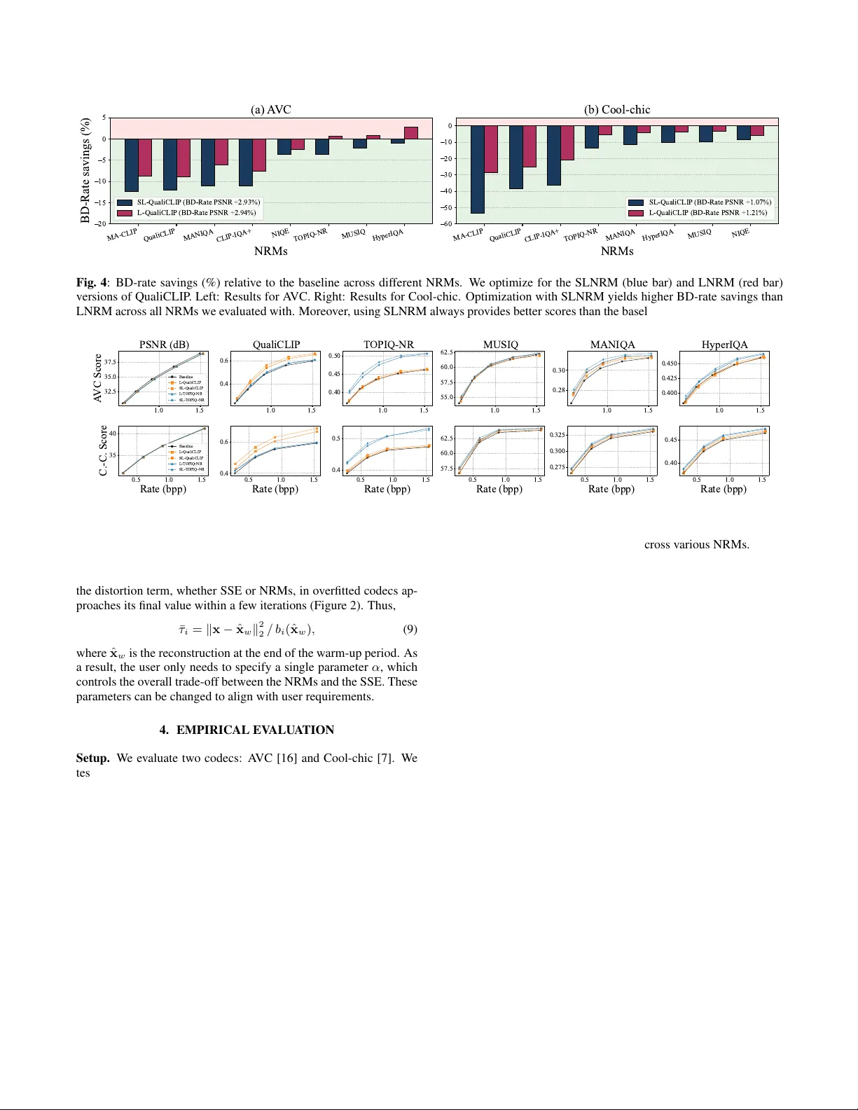
RA TE-DISTOR TION OPTIMIZA TION FOR ENSEMBLES OF NON-REFERENCE METRICS Xin Xiong S C * , Samuel F ern ´ andez-Mendui ˜ na S C * , Eduar do P avez S C , Antonio Orte ga S C , Neil Birkbeck G , Balu Adsumilli G S C Uni versity of Southern California, Los Angeles, CA, USA G Google Inc, Mountain V ie w , CA, USA ABSTRA CT Non-reference metrics (NRMs) can assess the visual quality of im- ages and videos without a reference, making them well-suited for the ev aluation of user -generated content. Nonetheless, rate-distortion optimization (RDO) in video coding is still mainly driven by full- reference metrics, such as the sum of squared errors, which treat the input as an ideal target. A way to incorporate NRMs into RDO is through linearization (LNRM), where the gradient of the NRM with respect to the input guides bit allocation. While this strategy improv es the quality predicted by some metrics, we sho w that it can yield limited gains or degradations when evaluated with other NRMs. W e argue that NRMs are highly non-linear predictors with locally unstable gradients that can compromise the quality of the linearization; furthermore, optimizing a single metric may exploit model-specific biases that do not generalize across quality estima- tors. Motiv ated by this observation, we extend the LNRM frame- work to optimize ensembles of NRMs and, to further improve ro- bustness, we introduce a smoothing-based formulation that stabilizes NRM gradients prior to linearization. Our frame work is well-suited to hybrid codecs, and we advocate for its use with overfitted codecs, where it av oids iterati ve ev aluations and backpropagation of neu- ral network–based NRMs, reducing encoder complexity relativ e to direct NRM optimization. W e v alidate the proposed approach on A VC and Cool-chic, using the Y ouTube UGC dataset. Experiments demonstrate consistent bitrate savings across multiple NRMs with no decoder complexity o verhead and, for Cool-chic, a substantial re- duction in encoding runtime compared to direct NRM optimization. Index T erms — Hybrid codec, RDO, gradient, linearization, non-reference quality assessment, Cool-chic 1. INTRODUCTION Non-reference metrics (NRMs) [1], which assess the perceptual quality of images and videos without a pristine reference, are im- portant for the compression of user-generated content (UGC) [2]. UGC is typically noisy due to motion blur , non-ideal e xposure, and artifacts from prior compression. Once uploaded to platforms like Y ouT ube and T ikT ok, UGC is re-encoded at different bitrates and resolutions to support adapti ve streaming [3]. In such pipelines, where the original content is unreliable, NRMs are popular for e val- uating perceptual quality [2, 4]. Despite their widespread adoption for quality e valuation, NRMs are still rarely used as bit-allocation objectiv es during compression [5]. Instead, rate-distortion optimiza- tion (RDO) in hybrid (i.e., block-based) [6] and o verfitted [7] codecs is mostly dri ven by full-reference metrics (FRMs), such as the sum of squared errors (SSE) [8], which assume the input is an ideal ref- erence. Hence, distortion con verges to perfect quality (as measured This work was funded in part by a Y ouT ube gift. *Equal contribution. by the FRM) as bitrate increases [5]. While appropriate for pristine content, FRMs encourage the preserv ation of artifacts when applied to UGC, which leads to suboptimal compression [9]. Thus, UGC setups can benefit from using NRMs in RDO. The strategy to incorporate them depends on the codec architecture. In ov erfitted codecs [7], the NRM can be included directly in the loss function and optimized end-to-end via gradient descent, as we sho w in Section 4. Howe ver, ov erfitted codecs require multiple ev alua- tions of the RD cost during encoding. Since modern NRMs are mostly implemented as deep neural networks, their repeated ev al- uation and backpropagation add substantial encoder complexity and runtime overhead [10]. For hybrid encoders, given that most NRMs map the input to a single value, obtaining per-pixel or per -block im- portance is not straightforward. As a result, RDO with NRMs for hybrid encoders may require iterativ e encoding, decoding, and met- ric ev aluation. T o address this issue, [5] proposed using the gradient of the metric ev aluated at the input to guide bit allocation, a strat- egy termed linearized NRM (LNRM), which drastically reduces the complexity of accounting for NRMs in hybrid codecs. While LNRM makes NRM-based RDO computationally effi- cient, NRMs are highly non-linear mappings from images to scalars, and their input gradients may exhibit local instability , i.e., the met- ric’ s response can vary sharply even for very small input changes [11]. Moreover , NRMs are imperfect quality estimators with model- specific biases, so that dif ferent NRMs produce different results for the same input. Experimentally , we observe, with both hybrid and ov erfitted codecs, that optimizing an LNRM deri ved from a specific (target) NRM often leads to significant improvements for the target NRM, while we observe marginal improvements (or e ven degrada- tions) for other NRMs (Figure 1). Although in some settings this might be desirable, gains that are more consistent across an ensemble of NRMs are more likely to reflect perceptual quality impro vements. In this work, we address these issues along two directions. First, we extend the LNRM formulation [5] to ensembles of metrics, thereby reducing sensitivity to the choice of NRM and encouraging improv ements across multiple, potentially unrelated quality predic- tors. Second, we introduce a smoothing-based optimization strategy , in which for a given NRM we average the scores obtained ov er small Gaussian perturbations of the input before linearization. This smoothed gradient strategy , similar to methods dev eloped in the machine learning literature [14, 15], computes an a verage of slightly perturbed gradients, attenuating sharp local variations and fa voring directions that remain stable under small input perturbations. This improv es the reliability of the first-order linearization underlying LNRM. Our approach can be incorporated into hybrid codecs, im- proving performance not only for the target NRMs but also across an ensemble of metrics. W e further argue for its use with ov erfitted codecs, where linearization substantially reduces encoding com- plexity relative to direct metric optimization. When combined with smoothing, further computational gains are obtained by av oiding (a) Input UGC (b) SSE (1.08 bpp) (c) QualiCLIP (1.09 bpp) QualiCLIP CLIP-IQA MA-CLIP HyperIQA MUSIQ BRISQUE 0.00 0.25 0.50 0.75 1.00 Normalized score (d) NRM scores Input UGC SSE QualiCLIP Fig. 1 : (a) Synthetic UGC obtained by compressing a KOD AK image [12] using JPEG [13] (with Q = 60 ). (b) Cool-chic reconstruction, optimizing for SSE (PSNR: 42 . 98 dB). (c) Cool-chic reconstruction, optimizing for QualiCLIP with SSE re gularization (PSNR: 42 . 63 dB). (d) Normalized scores (between 0 and 1 ) reported by multiple NRMs. While optimizing the bit-allocation for QualiCLIP impro ves the quality as predicted by some metrics, it yields limited improv ements or even de gradations in others. iterativ e ev aluations of the smoothed objectiv e. W e validate our framework using A VC [16] and Cool-chic [7] for se veral NRMs [17–19]. W e test frames sampled from the Y ouT ube UGC dataset [2], setting the RDO to optimize dif ferent NRMs using our approach, considering both ensembles of metrics and smoothed objectiv es. For Cool-chic, we also consider direct NRM optimization. Results in Section 4 sho w that our method can yield impro vements in div erse NRMs, with no decoder complex- ity ov erhead and, for Cool-chic, a substantial reduction in runtime relativ e to optimizing the NRM directly . 2. PRELIMINARIES Notation. Uppercase and lowercase bold letters, such as A and a , denote matrices and vectors, respectively . The n th entry of the vector a is a n . Regular letters denote scalar v alues. 2.1. Rate-distortion optimization Both h ybrid [16, 20] and overfitted [7] codecs aim to find parameters θ θ θ that optimize a rate-distortion (RD) cost. Given x , an input with n p pixels, and ˆ x ( θ θ θ ) , its compressed version with parameters θ θ θ , full- reference RDO aims at minimizing: J ( ˆ x ( θ θ θ )) = d ( ˆ x ( θ θ θ ) , x ) + λ r ( ˆ x ( θ θ θ )) , (1) where d ( · , · ) denotes the distortion metric, r ( · ) the bitrate, and λ controls the RD trade-of f. For the purpose of this paper, the k ey difference between hybrid and o verfitted codecs is the domain of the coding parameters θ θ θ and optimization strategy used to minimize (1). Hybrid codecs. The parameters θ θ θ = [ θ 1 , . . . , θ n b ] ∈ N n b take discrete values, which may represent block partitioning, prediction mode, or quantization step. Giv en a distortion term that splits block- wise d ( ˆ x ( θ θ θ ) , x ) = P n b i =1 d i ( ˆ x i ( θ i ) x i ) , e.g., the sum of squared errors (SSE), where x i is the i th block of the input and ˆ x i ( θ i ) its compressed version with parameters θ i , we have block lev el RDO: θ ⋆ i = arg min θ i d i ( ˆ x i ( θ i ) , x i ) + λ r ( ˆ x i ( θ i )) . Overfitted codecs. W e focus on Cool-chic [7]. The continuous pa- rameters θ θ θ , namely , the latent representation of the image, the en- tropy coding parameters, and the weights of the synthesis CNN, are optimized via gradient descent. Since quantization and entropy cod- ing are not differentiable [21], a dif ferentiable approximation of the RD cost in (1) is used instead. The parameters are updated o ver thousands of iterations using this cost, which must be evaluated and backpropagated at e very iteration. 2.2. Linearized NRM A method to perform RDO with hybrid codecs using a NRM as dis- tortion metric was proposed in [5]. Let the NRM be b ( · ) . Then, θ θ θ ⋆ = arg min θ θ θ b ( ˆ x ( θ θ θ )) + τ ∥ x − ˆ x ∥ 2 2 + λ r ( ˆ x ( θ θ θ )) , (2) where τ controls the SSE-NRM trade-of f. When the metric is dif- ferentiable and the gradients exist, a first order T aylor expansion to b ( ˆ x ( θ θ θ )) around the input image x yields θ θ θ ⋆ = arg min θ θ θ ∇ b ( x ) ⊤ ( ˆ x ( θ θ θ ) − x ) + τ ∥ x − ˆ x ∥ 2 2 + λ r ( ˆ x ( θ θ θ )) . (3) The term ∇ b ( x ) ⊤ ( ˆ x ( θ θ θ ) − x ) is called linearized NRM (LNRM). The dependence on the compressed image is linear , which implies that the metric can be ev aluated block-wise in hybrid codecs. 3. OPTIMIZA TION WITH NRM Since the gradient in (3) depends only on the input image, the NRM needs to be evaluated (and backpropagated) only once. W e lev erage this property to optimize efficiently for ensembles of NRMs. 3.1. Ensembles of metrics W e consider an ensemble of metrics, ℓ c ( x ) . = P n m i =1 τ i b i ( x ) , where b i ( · ) is the i th NRM and τ i is the corresponding weight. By applying a first-order T aylor expansion around x , we obtain: ℓ c ( ˆ x ( θ θ θ )) = ℓ c ( x ) + ∇ ℓ c ( x ) ⊤ ( ˆ x ( θ θ θ ) − x ) + o ( ∥ ˆ x ( θ θ θ ) − x ∥ 2 2 ) , (4) where the ensemble gradient satisfies ∇ ℓ c ( x ) = P n m i =1 τ i ∇ b i ( x ) . Thus, we can optimize for an ensemble of metrics by 1) ev aluating each NRM and then computing the gradient of the metric with re- spect to the input, and 2) ev aluating an LNRM based on the weighted av erage of the gradients. LNRMs decouple NRM ev aluation from the coding loop: we construct and optimize an LNRM for each input and ensemble of NRMs. As a result, ev aluating the LNRM during encoding is inexpensi ve once the gradients are av ailable. Ensemble composition. Since different NRMs may capture differ - ent and weakly correlated properties of the image, one way to con- struct the ensemble is to complement these behaviors rather than re- inforce a single notion of quality . Thus, the ensemble will promote improv ements that are consistent across div erse and partially inde- pendent NRMs. T o this end, we analyze the correlation between the scores produced by dif ferent NRMs ov er a set of images. Given 0.0 0.5 1.0 I t e r a t i o n ( × 1 0 4 ) 0.0 0.5 1.0 1.5 2.0 M S E ( × 1 0 3 ) (a) MSE vs Iteration MSE 0.0 0.5 1.0 I t e r a t i o n ( × 1 0 4 ) 0.8 1.0 1.2 1.4 Rate (bpp) (b) Rate (bpp) vs Iteration Rate (bpp) 0.0001 0.0004 0.001 0.004 Lambda 0.0 0.2 0.4 0.6 0.8 1.0 Score (c) T OPIQ-NR W arm-up Final 0.0001 0.0004 0.001 0.004 Lambda 0.0 0.2 0.4 0.6 0.8 1.0 Score (d) QualiCLIP W arm-up Final Fig. 2 : (a) MSE and (b) rate evolution across iterations for Cool-chic in one image. While the MSE con verges fast, the decrease in rate is more gradual. (c-d) A verage NRM score (50 images), showing warm-up reconstructions achie ve near-final scores, justifying (9). a dataset of compressed reconstructions at various bitrates, we com- pute pairwise correlations between metric outputs. Metrics with high correlation tend to respond similarly to changes in compression pa- rameters and may provide redundant guidance during optimization. Con versely , metrics with low correlation are more likely to capture complementary properties. W e sho w an example in Figure 3 and provide guidance on ho w to choose the weights τ i in Section 3.4. 3.2. Smoothed LNRM An approach to improve the robustness of the LNRM framework is to smooth the metric prior to linearization [14]. Giv en σ > 0 , b σ ( x ) . = E n ∼N (0 ,σ 2 I )  b ( x + n )  . Smoothing re gularizes the metric by attenuating high-curvature components of its response surface, yielding a function with better local smoothness properties [14]. Moreov er, since ∇ b σ ( x ) = E n  ∇ b ( x + n )  , the smoothed gradient is an average of perturbed gradients, fa voring directions that remain stable under small perturbations of the input, which emphasizes fea- tures that may generalize better across multiple quality predictors. W e use a Monte Carlo approximation with n s samples: b σ ( x ) = n s X i =1 1 /n s b ( x + n i ) , with n i ∼ N ( 0 , σ I ) , (5) and σ is chosen such that the noise is imperceptible for a human observer [15]. Applying the same T aylor expansion around x as in (4), we obtain a LNRM with the smoothed version of the gradient: ∇ b σ ( x ) = n s X i =1 1 /n s ∇ b ( x + n i ) . (6) Then, ∇ b σ ( x ) ⊤ ( ˆ x ( θ θ θ ) − x ) is the smoothed LNRM (SLNRM). Since linearization decouples NRM evaluation from bit allocation, SLNRM still adds only limited complexity . Howe ver, the setup cost is higher for SLNRM: the initial LNRM requires only one backpropagation, while SLNRM requires n s . 3.3. LNRM with overfitted codecs LNRMs (3) can be applied to ove rfitted codecs. In this case, the main motiv ation is computational: optimizing the LNRM is much 0.2 0.0 0.2 0.4 MDS dimension 1 0.2 0.0 0.2 MDS dimension 2 QualiCLIP MA-CLIP CLIP-IQA+ MANIQA T OPIQ-NR HyperIQA MUSIQ NIQE Fig. 3 : Multidimensional scaling (MDS) [22] for NRM correlation. W e show d i,j = 1 − | p i,j | , with p i,j the 2D projection of the rank correlation between NRMs i and j . W e identify three clusters. cheaper than optimizing the corresponding NRM. W e focus on the complexity of a Cool-chic encoder with n i iterations. Let n f be the number of FLOPs/px needed to compute a target NRM. Let n s be the number of smoothgrad samples. Since computing the gradient is twice as complex as ev aluating the metric [5], the complexity over- head due to the NRM is 3 × n i × n f FLOPs/px, which increases to 3 × n i × n f × n s FLOPs/px when we consider smoothing. On the other hand, the complexity of ev aluating the LNRM splits into two parts: computing the gradient, with complexity 3 × n f , and ev aluating the LNRM on each iteration, with complexity 2 n i FLOPs/px. For SLNRM, only the complexity of computing the gra- dient increases: we require 3 × n f × n s FLOPs/px to obtain the smoothed gradient. Hence, relying on the LNRM reduces the com- putational complexity by a factor of approximately n i . The number of iterations in Cool-chic is of the order of 10 4 ; hence, the LNRM can reduce complexity by orders of magnitude. Section 4 shows that complexity impro vements also translate to runtime improvements. 3.4. SSE regularization As in [5], we complement the LNRM with a SSE regularizer . T o av oid modifying the Lagrangian, we constrain the SSE-based setup: θ θ θ ⋆ = arg min θ θ θ ∈ Θ ∥ ˆ x ( θ θ θ ) − x ∥ 2 2 + λ n b X i =1 r i ( ˆ x i ( θ i )) , suc h that ∇ ℓ c ( x ) ⊤ ( ˆ x ( θ θ θ ) − x ) ≤ LNRM max , (7) where LNRM max is the maximum acceptable LNRM value. By applying Lagrangian relaxation [23], we can write: d ( x , ˆ x ( θ θ θ )) = ∥ x − ˆ x ∥ 2 2 + n m X i =1 τ i ∇ b i ( x ) ⊤ ( ˆ x − x ) , (8) where τ i can be selected by the user to control the trade-off be- tween performance among SSE and the different NRMs. T o decide on the weights for each metric, we follow [5]: we split τ i = α ¯ τ i . Our choice of ¯ τ varies depending on the type of codec. For hy- brid codecs, we choose ¯ τ i = p n p / 12 ∆ / ∥∇ b i ( x ) ∥ 2 , for all i = 1 , . . . , n m , since it balances the SSE and LNRM contributions to the total cost for the smallest possible quantization error [5]. Over- fitted codecs lack an explicit quantization step, so we cannot use the same relationship. Instead, we lev erage the warm-up process to ob- tain estimates of both quantities. W e hav e empirically found that MA-CLIP QualiCLIP MANIQA CLIP-IQA+ NIQE T OPIQ-NR MUSIQ HyperIQA NRMs 20 15 10 5 0 5 BD-Rate savings (%) (a) A VC SL-QualiCLIP (BD-Rate PSNR +2.93%) L-QualiCLIP (BD-Rate PSNR +2.94%) MA-CLIP QualiCLIP CLIP-IQA+ T OPIQ-NR MANIQA HyperIQA MUSIQ NIQE NRMs 60 50 40 30 20 10 0 (b) Cool-chic SL-QualiCLIP (BD-Rate PSNR +1.07%) L-QualiCLIP (BD-Rate PSNR +1.21%) Fig. 4 : BD-rate savings (%) relativ e to the baseline across dif ferent NRMs. W e optimize for the SLNRM (blue bar) and LNRM (red bar) versions of QualiCLIP . Left: Results for A VC. Right: Results for Cool-chic. Optimization with SLNRM yields higher BD-rate savings than LNRM across all NRMs we ev aluated with. Moreover , using SLNRM always pro vides better scores than the baseline reg ardless of the NRM. 1.0 1.5 32.5 35.0 37.5 A VC Score PSNR (dB) Baseline L-QualiCLIP SL-QualiCLIP L-T OPIQ-NR SL-T OPIQ-NR 1.0 1.5 0.4 0.6 QualiCLIP 1.0 1.5 0.40 0.45 0.50 T OPIQ-NR 1.0 1.5 55.0 57.5 60.0 62.5 MUSIQ 1.0 1.5 0.28 0.30 MANIQA 1.0 1.5 0.400 0.425 0.450 HyperIQA 0.5 1.0 1.5 Rate (bpp) 35 40 C.-C. Score Baseline L-QualiCLIP SL-QualiCLIP L-T OPIQ-NR SL-T OPIQ-NR 0.5 1.0 1.5 Rate (bpp) 0.4 0.6 0.5 1.0 1.5 Rate (bpp) 0.4 0.5 0.5 1.0 1.5 Rate (bpp) 57.5 60.0 62.5 0.5 1.0 1.5 Rate (bpp) 0.275 0.300 0.325 0.5 1.0 1.5 Rate (bpp) 0.40 0.45 Fig. 5 : Rate-quality curves comparing baseline, LNRM, and SLNRM evalua ted across various NRMs. T op: the results for A VC; Bottom: the results for Cool-chic. In each sub-figure, the black curve represents the baseline. Other colors correspond to RDO using specific NRMs, where solid lines indicate LNRM and dashed lines indicate SLNRM. SLNRM consistently outperforms LNRM across various NRMs. the distortion term, whether SSE or NRMs, in ov erfitted codecs ap- proaches its final value within a fe w iterations (Figure 2). Thus, ¯ τ i = ∥ x − ˆ x w ∥ 2 2 / b i ( ˆ x w ) , (9) where ˆ x w is the reconstruction at the end of the warm-up period. As a result, the user only needs to specify a single parameter α , which controls the ov erall trade-off between the NRMs and the SSE. These parameters can be changed to align with user requirements. 4. EMPIRICAL EV ALU A TION Setup. W e ev aluate two codecs: A VC [16] and Cool-chic [7]. W e test 50 frames of 640 × 480 pixels, sampled from the Y ouT ube UGC dataset [2]. W e use 4:4:4 A VC baseline [5] with QP ∈ { 25 , 28 , 31 , 34 , 37 } . QP offset for color channels is 3 . W e use RDO to choose block partition ( 4 × 4 and 16 × 16 ) and block-level quantization step ( ∆QP = − 4 , − 3 , . . . , 3 , 4 ). For computing ¯ τ in Section 3.4, we set ∆(QP) = 2 (QP − 4) / 6 [24]. For Cool-chic, we use the fast training profile ( 10 4 iterations) with λ values of 0.004, 0.001, 0.0004 and 0.0001. W e use an AMD 9950X3D CPU with a NVIDIA Geforce R TX 5090 (32GB VRAM). The baseline is the version of each codec optimizing the SSE during RDO. W e ev aluate on QualiCLIP [18], TOPIQ-NR [17], CLIP-IQA+ [25], MANIQA [26], MUSIQ [27], NIQE [1], MA-CLIP [28], and HyperIQA [29] with default settings [30]. For ensemble optimiza- tion, we analyze the NRM correlation (Figure 3) by assessing re- construction quality using SSE-RDO A VC across 5 QP values. W e identify three clusters; since one cluster only has one metric (NIQE), we select a NRM from the other two (T OPIQ-NR, QualiCLIP). Coding experiments. W e e valuate LNRM and SLNRM across mul- tiple target NRMs. For smoothing, we set n s = 5 and σ = 0 . 01 . Figure 4 illustrates the average BD-rate savings on various NRMs when optimizing for QualiCLIP via LNRM and SLNRM. W e tune the hyperparameter α to make the BD-rate loss for PSNR com- parable across all methods, implying that the degradation in SSE is similar across all methods. Under this condition, SLNRM con- sistently achie ves higher bitrate savings than LNRM, not only for the target NRM but also across other ev aluated metrics. W e ob- serve that the coding gains for Cool-chic are larger than those for A VC, which we attribute to the larger optimization space av ailable on Cool-chic. F or A VC (T able 1), when optimizing for a single LNRM, performance is superior when e valuated on NRMs within the same cluster (cf. Figure 3). When combining two target NRMs from the same cluster (e.g., QualiCLIP and CLIP-IQA+), we observe performance improvements on CLIP-IQA+ relativ e to using Quali- CLIP only; howev er , gains on other metrics are negligible. Con- versely , when combining metrics from different clusters (e.g., Qual- iCLIP and TOPIQ-NR), we observe performance improv ements in the TOPIQ-NR cluster relative to using QualiCLIP alone. Applying smoothing to these combinations also yields broad improvements across all ev aluated metrics. For Cool-chic, we extend our analysis to include direct optimization of both the NRM and its smoothed version. As shown in Figure 6, when optimizing and ev aluating for QualiCLIP , directly optimizing the NRM yields the best per- formance, whereas the smoothed NRM shows a slight degradation. Y et, when ev aluating NRMs from different clusters (T able 2), the smoothed NRM outperforms direct NRM optimization. These re- sults suggest that optimizing the smoothed metric directly also im- T able 1: BD-rate savings (%) relati ve to SSE-RDO A VC. Comparison of multiple LNRM and SLNRM pairs. SLNRM outperforms LNRM across various NRMs at comparable PSNR drops. Ensemble 1: QualiCLIP+CLIPIQA+, ensemble 2: QualiCLIP+ TOPIQ-NR. Method PSNR QualiCLIP MA-CLIP CLIP-IQA+ TOPIQ-NR MANIQA MUSIQ HyperIQA NIQE L-QualiCLIP 2.94 -8.81 -8.64 -7.61 0.63 -6.09 0.88 2.81 -2.47 SL-QualiCLIP 2.93 -12.09 -12.37 -10.98 -3.53 -11.06 -2.19 -0.92 -3.63 L-TOPIQ-NR 3.28 -2.51 -2.37 -4.07 -22.56 -10.85 -1.85 -6.25 -2.77 SL-TOPIQ-NR 3.26 -2.93 -3.60 -4.54 -27.20 -15.93 -3.00 -9.06 -2.33 L-Ensemble 1 2.97 -8.30 -8.66 -10.65 0.10 -5.57 1.09 1.62 -2.25 SL-Ensemble 1 3.01 -11.41 -12.33 -14.37 -4.62 -11.05 -4.01 -2.35 -3.00 L-Ensemble 2 3.01 -7.45 -6.97 -6.93 -19.49 -11.50 -1.30 -4.73 -2.86 SL-Ensemble 2 3.00 -10.49 -10.84 -10.11 -24.14 -18.35 -6.76 -9.32 -3.83 T able 2: BD-rate savings (%) relativ e to SSE-based Cool-chic. As with A VC, SLNRM consistently outperforms LNRM, and optimizing for the smoothed NRM outperforms optimizing for the NRM in the ensemble. When optimizing and e valuating with the same NRM, reconstructions may hav e no-overlapping RD curv es with inv alid BD-rates (dashed cases). W e report the RD curves for these cases in Figure 6. Method PSNR QualiCLIP MA-CLIP CLIP-IQA+ TOPIQ-NR MANIQA MUSIQ HyperIQA NIQE L-QualiCLIP 1.21 -25.14 -28.59 -20.76 -5.50 -4.19 -3.14 -3.59 -5.82 SL-QualiCLIP 1.07 -38.56 -53.37 -36.01 -13.52 -11.19 -9.53 -10.07 -8.25 QualiCLIP 0.82 — — — -10.88 -10.42 -6.97 -7.27 -7.44 S-QualiCLIP 0.75 — — — -17.57 -16.50 -11.09 -15.09 -6.28 L-TOPIQ-NR 0.95 -5.66 -3.61 -5.41 -43.07 -13.34 -7.25 -14.56 -3.52 SL-TOPIQ-NR 1.07 -6.90 -15.01 -6.35 -49.24 -17.01 -14.43 -17.92 -2.41 T able 3: BD-rate savings (%) relativ e to SSE-RDO A VC as a func- tion of smoothing parameters ( n s and noise le vel σ ). W e optimize for SL-QualiCLIP . n s = 5 and σ = 0 . 01 yields gains in all metrics. n s , σ PSNR QualiCLIP CLIP-IQA+ MUSIQ MANIQA HyperIQA 5,0.005 2.74 -11.27 -9.65 0.32 -8.06 0.72 5,0.01 2.93 -12.09 -10.98 -2.19 -11.06 -0.92 10,0.005 2.93 -11.56 -10.45 -0.04 -7.91 0.15 10,0.01 2.89 -12.72 -11.52 -3.13 -12.72 -2.12 20,0.005 3.05 -11.67 -9.82 -0.80 -8.26 -0.37 20,0.01 2.91 -12.73 -11.47 -3.35 -11.85 -3.26 T able 4: Runtime of gradient computation and Cool-chic encoding with LNRM, SLNRM, and NRM. Gradient computation time is re- ported in milliseconds (ms), while encoding time is shown as the ov erhead relativ e to the baseline ( ≈ 50 s). Encoding with NRM in- troduces significant ov erhead compared to LNRM and SLNRM. Gradient compute (ms) Cool-chic encoding overhead (%) NRMs LNRM SLNRM LNRM SLNRM NRM QualiCLIP 7 28 +2.6% +2.8% +196% TOPIQ-NR 17 63 +1.8% +2.6% +457% prov es performance in ensembles of NRMs. Ablations (T able 3). W e test smoothing parameters with QualiCLIP . W e observe that n s = 5 provides a good trade-off between perfor- mance and computational overhead. Increasing n s yields marginal gains, with performance saturation beyond n s = 10 . Since the computational cost of smoothing scales linearly with n s , we adopt n s = 5 for our experiments. W e also evaluate the impact of noise intensity with σ = 0 . 005 and σ = 0 . 01 . The visual impact of the added noise is negligible, with PSNR values relative to the input UGC image of 46 . 1 dB and 40 . 1 dB, respectiv ely . A larger σ ( 0 . 01 ) leads to better coding gains across all the e valuated NRMs. Runtime analysis (T able 4). W e sho w the runtime for gradient com- putation and Cool-chic encoding with LNRM, SLNRM, and NRM 0.5 1.0 1.5 Rate (bpp) 35 40 C.-C. Score PSNR (dB) Baseline L-QualiCLIP SL-QualiCLIP QualiCLIP S-QualiCLIP 0.5 1.0 1.5 Rate (bpp) 0.4 0.6 0.8 QualiCLIP 0.5 1.0 1.5 Rate (bpp) 0.5 0.6 CLIP-IQA+ Fig. 6 : Rate-quality curves for Cool-chic. Using the NRM as a dis- tortion metric in RDO performs best when ev aluated by the same NRM. The SLNRM outperforms the LNRM in the giv en metric. for fiv e images with two λ values. The experiment is repeated twice with two random seeds. Though computing smoothed gradients with n s = 5 increases complexity by approximately 5 times, this over - head is ne gligible relati ve to the Cool-chic encoding time (around 50 seconds per image in our setup). Hence, the difference in encoding runtime between LNRM and SLNRM is minimal. Directly optimiz- ing for NRM incurs a substantial runtime penalty , since the NRM must be ev aluated at each iteration. 5. CONCLUSION In this paper , we showed that optimizing for a single NRM leads to inconsistent behavior when evaluated with other NRMs. T o address this, we proposed an RDO frame work based on LNRMs that enables optimization over ensembles of metrics. Building on this formula- tion, we introduced a smoothing-based approach inspired by robust optimization, which improves performance not only on the target metric but also in other NRMs while exploiting the computational advantages of linearization. Experiments with A VC and Cool-chic on the Y ouTube UGC dataset demonstrate consistent bitrate savings across di verse NRMs, reduced sensiti vity to the choice of NRM, and substantial encoder runtime reductions compared to direct NRM op- timization for Cool-chic, with no decoder-side overhead. While we focused on image compression, the proposed framew ork naturally extends to video coding by incorporating video NRMs. 6. REFERENCES [1] A. Mittal, R. Soundararajan, and A. C. Bovik, “Making a “completely blind” image quality analyzer , ” IEEE Signal Pro- cessing Letters , vol. 20, no. 3, pp. 209–212, 2013. [2] Y . W ang, S. Inguva, and B. Adsumilli, “Y ouTube UGC dataset for video compression research, ” in Pr oc. IEEE Intl. W ork. on Mult. Signal Pr ocess. IEEE, 2019, pp. 1–5. [3] M. Seufert, S. Egger, M. Slanina, T . Zinner , T . Hoßfeld, and P . T ran-Gia, “ A survey on quality of e xperience of HTTP adap- tiv e streaming, ” IEEE Comms. Surv . & T utor . , vol. 17, no. 1, pp. 469–492, 2014. [4] E. Pavez, E. Perez, X. Xiong, A. Ortega, and B. Adsumilli, “Compression of user generated content using denoised refer- ences, ” in Pr oc. IEEE Int. Conf. Image Pr ocess. IEEE, 2022, pp. 4188–4192. [5] S. Fern ´ andez-Mendui ˜ na, X. Xiong, E. Pav ez, A. Ortega, N. Birkbeck, and B. Adsumilli, “Rate-distortion optimization with non-reference metrics for UGC compression, ” in Proc. IEEE Int. Conf. Image Pr ocess. , 2025, pp. 2372–2377. [6] G. J. Sulli van and T . W iegand, “Rate-distortion optimization for video compression, ” IEEE Signal Pr ocess. Mag. , vol. 15, no. 6, pp. 74–90, 1998. [7] T . Ladune, P . Philippe, F . Henry , G. Clare, and T . Leguay , “Cool-chic: Coordinate-based low complexity hierarchical im- age codec, ” in Pr oc. IEEE/CVF Int. Conf. Comput. V is. , 2023. [8] A. Ortega and K. Ramchandran, “Rate-distortion methods for image and video compression, ” IEEE Signal Pr ocess. Mag. , vol. 15, no. 6, pp. 23–50, No v . 1998. [9] X. Xiong, E. Pav ez, A. Ortega, and B. Adsumilli, “Rate- distortion optimization with alternativ e references for UGC video compression, ” in Pr oc. IEEE Int. Conf. Acoust., Speech, and Signal Pr ocess. , 2023, pp. 1–5. [10] P . Philippe, T . Ladune, G. Clare, and F . E. Henry , “Perceptu- ally optimised cool-chic for clic 2025, ” in 7th Challenge on Learned Image Compression . [11] Y . Liu, C. Y ang, D. Li, J. Ding, and T . Jiang, “Defense against adversarial attacks on no-reference image quality models with gradient norm regularization, ” in Proc. IEEE/CVF Conf. on Comp. V is. and P att. Recog. , 2024, pp. 25554–25563. [12] E. Kodak, “Kodak loss less true color image suite, ” 1993. [13] G. K. W allace, “The JPEG still picture compression standard, ” Communications of the ACM , v ol. 34, no. 4, pp. 30–44, 1991. [14] J. Cohen, E. Rosenfeld, and Z. Kolter , “Certified adversarial robustness via randomized smoothing, ” in Proc. Intl. Conf. Mach. Learn. PMLR, 2019, pp. 1310–1320. [15] D. Smilkov , N. Thorat, B. Kim, F . V i ´ egas, and M. W attenberg, “Smoothgrad: removing noise by adding noise, ” arXiv preprint arXiv:1706.03825 , 2017. [16] T . W iegand, G. Sulliv an, G. Bjonteg aard, and A. Luthra, “Overvie w of the H.264/A VC video coding standard, ” IEEE T rans. Circuits Syst. V ideo T echnol. , vol. 13, no. 7, pp. 560– 576, July 2003. [17] C. Chen, J. Mo, J. Hou, H. W u, L. Liao, W . Sun, Q. Y an, and W . Lin, “T opiq: A top-down approach from semantics to dis- tortions for image quality assessment, ” IEEE T rans. Image Pr ocess. , vol. 33, pp. 2404–2418, 2024. [18] L. Agnolucci, L. Galteri, and M. Bertini, “Quality-aware image-text alignment for opinion-unaware image quality as- sessment, ” arXiv preprint , 2024. [19] W . Zhang, K. Ma, J. Y an, D. Deng, and Z. W ang, “Blind image quality assessment using a deep bilinear con volutional neural network, ” IEEE T rans. Cir cuits Syst. V ideo T echnol. , vol. 30, no. 1, pp. 36–47, 2020. [20] B. Bross, Y .-K. W ang, Y . Y e, S. Liu, J. Chen, G. J. Sulli van, and J.-R. Ohm, “Overvie w of the versatile video coding (VVC) standard and its applications, ” IEEE T rans. Circuits Syst. V ideo T ec hnol. , vol. 31, no. 10, pp. 3736–3764, 2021. [21] J. Ball ´ e, V . Laparra, and E. P . Simoncelli, “End-to-end opti- mized image compression, ” pr eprint arXiv:1611.01704 , 2016. [22] J. B. Kruskal, “Multidimensional scaling by optimizing good- ness of fit to a nonmetric hypothesis, ” Psychometrika , vol. 29, no. 1, pp. 1–27, 1964. [23] H. Everett III, “Generalized Lagrange multiplier method for solving problems of optimum allocation of resources, ” Opera- tions resear ch , vol. 11, no. 3, pp. 399–417, 1963. [24] S. Ma, W . Gao, D. Zhao, and Y . Lu, “ A study on the quantiza- tion scheme in H. 264/A VC and its application to rate control, ” in Pr oc. P ac. Rim Conf. on Mult., P art III 5 . Springer , 2004, pp. 192–199. [25] J. W ang, K. C. Chan, and C. C. Loy , “Exploring clip for as- sessing the look and feel of images, ” in AAAI , 2023. [26] S. Y ang, T . W u, S. Shi, S. Lao, Y . Gong, M. Cao, J. W ang, and Y . Y ang, “Maniqa: Multi-dimension attention network for no-reference image quality assessment, ” in Pr oc. IEEE/CVF Conf. Comput. V is. P attern Recog. , 2022, pp. 1191–1200. [27] J. Ke, Q. W ang, Y . W ang, P . Milanfar , and F . Y ang, “Musiq: Multi-scale image quality transformer, ” in Proc. IEEE/CVF Int. Conf. Comput. V is. , 2021, pp. 5148–5157. [28] Z. Liao, D. W u, Z. Shi, S. Mai, H. Zhu, L. Zhu, Y . Jiang, and B. Chen, “Beyond cosine similarity magnitude-aware clip for no-reference image quality assessment, ” arXiv preprint arXiv:2511.09948 , 2025. [29] S. Su, Q. Y an, Y . Zhu, C. Zhang, X. Ge, J. Sun, and Y . Zhang, “Blindly assess image quality in the wild guided by a self- adaptiv e hyper network, ” in Pr oc. IEEE/CVF Conf. Comput. V is. P attern Recog. , June 2020. [30] C. Chen and J. Mo, “IQA-PyT orch: Pytorch toolbox for image quality assessment, ” 2022.