Reproducibility and Statistical Methodology

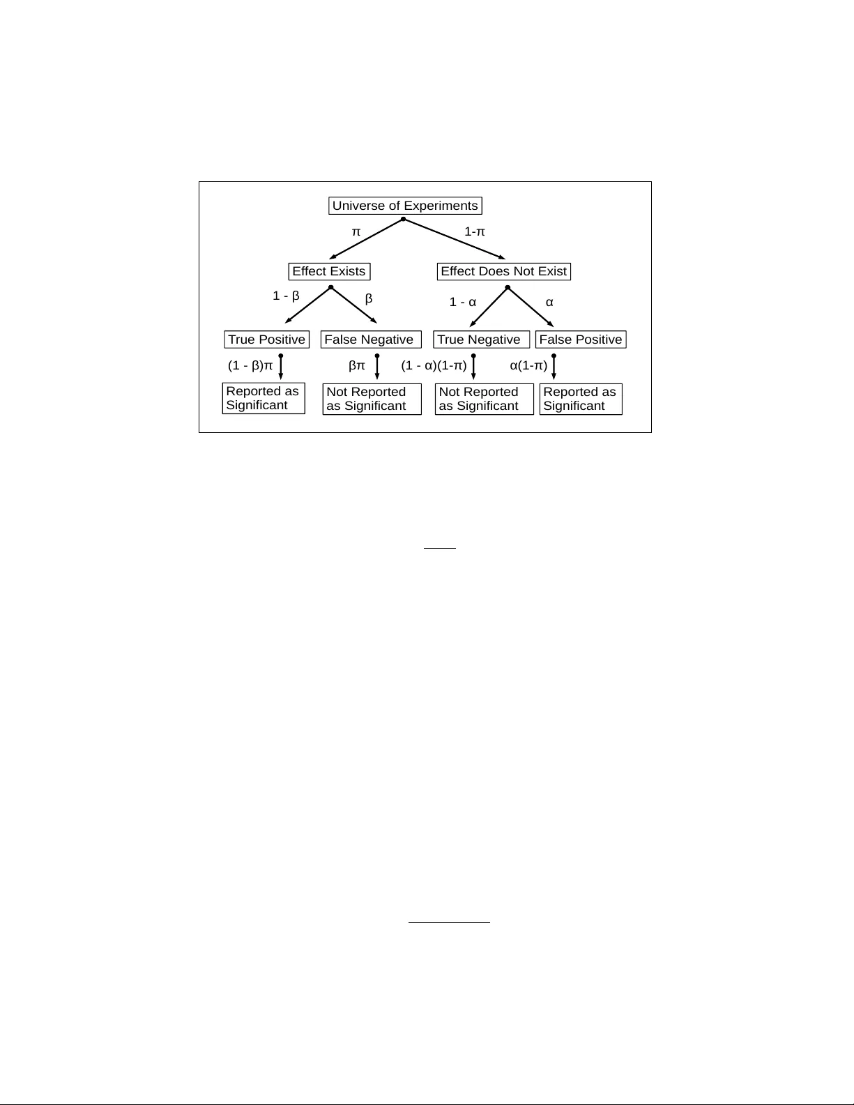
Repro ducibilit y and Statistical Metho dology An thony Alm udev ar, PhD Departmen t of Biostatistics and Computational Biology , Univ ersity of Ro chester, Ro c hester NY Jacob Almudev ar, MSc Departmen t of Mathematics and Statistics, Univ ersity of New Hampshire, Durham NH F ebruary 18, 2026 Abstract. In 2015 the Op en Science Collab oration (OSC) (Nosek et al 2015) published a highly influen tial pap er whic h claimed that a large fraction of published results in the psyc hological sciences were not repro ducible. In this article we review this claim from several p oin ts of view. W e first offer an extended analysis of the metho ds used in that study . W e sho w that the OSC methodology induces a bias that is able by itself to explain the discrepancy b et ween the OSC estimates of reproducibility and other more optimistic estimates made b y similar studies. The article also offers a more general literature review and discussion of repro ducibilit y in exp erimental science. W e argue, for b oth scientific and ethical reasons, that a considered balance of false p ositiv e and false negative rates is preferable to a single-minded concen tration on false p ositiv e rates alone. 1 In tro duction The v alue of any kind of research depends on the repro ducibilit y of the results. “The salutary habit,” suggests Ronald Fisher, “of rep eating im- p ortan t exp eriments, or of carrying out original observ ations in replicate, sho ws a tacit appreciation of the fact that the ob ject of our study is not the individual result, but the p opulation of possibilities of which we do our b est to make our exp erimen ts representativ e.” (Fisher, 1925). 1 If a study pro duces an outcome whic h cannot b e repro duced in a sim- ilar environmen t at another p oin t in time, then such a s tudy has failed in its original goal to pro vide observ ations that allude to real-life phenomena. Therefore, ensuring the repro ducibility of all studies is a top priority in all fields of science. Ho wev er, a num b er of inv estigations into the curren t cli- mate of scien tific studies hav e suggested that a large num b er of published results are unable to be reproduced, implying that these results ha v e no implications outside of the initial test conditions. This issue is known in the literature as the r epr o ducibility (or r eplic ation ) crisis , and has become a significan t concern. In fact, according to a surv ey of researchers rep orted in Baker (2016) “ ... 52% of those survey ed agree that there is a significan t ‘crisis’ of repro ducibilit y ...”. As a consequence, failure of repro ducibilit y is seen as a ma jor issue across most fields of science, with many individuals and organizations inv estigating these claims. In order to test this, the Open Science Collab oration (OSC) ( osf.io/vmrgu ) conducted a replication pro ject (OSC-RP), selecting 100 studies from promi- nen t psyc hological journals and repro ducing them in close to original con- ditions (Nosek et al. , 2015). The OSC-RP rep orts that while 97% of the original exp erimen ts were sho wn to hav e significant results ( P ≤ 0 . 05), of these only 36% of the reproduced exp erimen ts were found to b e significant under similar conditions. F urthermore, 47% of effect sizes from the original exp erimen ts w ere within the 95% confidence in terv al of the effect sizes from repro duced studies, and 39% of effects were sub jectively considered to b e successful repro ductions. The OSC-RP rep ort do es not discern any particular systematic flaws in exp erimental or statistical methodology , although it conjectures issues regarding incen tive in the scientific communit y . The OSC-RP do es conclude, ho wev er, and implies as suc h in their rep ort, that the scien tific comm unity faces a self-evident risk of irrepro ducible and unreliable experimental data from ma jor scientific journals. If true, this is a serious concern that requires some degree of reform in exp erimen tation and publication practices. Ho wev er, not all studies of repro ducibility yield p essimistic conclusions. Etz and V andek erc khov e (2016) presen ts the notion that the rep orted fail- ure of repro ducibilit y from the OSC-RP’s rep ort can b e attributed to an “o verestimation of effect sizes”. Klein et al. (2014) summarizes a separate replication study , the Man y Labs Replication Pro ject (ML-RP), whic h re- p orted a m uch higher reproducibility rate of 85%, one compatible with strict adherence to go o d exp erimen tal and statistical practice ( https://osf.io/ wx7ck/k/ ). In a similar study reported in Camerer et al. (2016) 18 exp er- imen tal studies in the field of economics were replicated, again yielding a 2 higher repro ducibility rate than the OSC-RP (61%), while using a similar replication proto col (ECO-RP). See also the exc hange in Gilb ert et al. (2016) and Anderson et al. (2016) following publication of Nosek et al. (2015). Therefore, there may be a different conclusion to discern from the statis- tical data presen ted b y the OSC-RP , one that is b oth sensible and elemen tary in regards to basic statistical principles. In order to inv estigate further, we m ust b egin b y clarifying and reconsidering the degree of repro ducibilit y that researc hers should exp ect from such studies. 2 A simple mathematical mo del for repro ducibil- it y W e first develop a “repro ducibilit y mo del” with which to precisely define a repro ducibilit y rate and to offer guidance regarding its estimation. Through- out, mo del assumptions will nev er deviate from standard practice, and w e will assume, in particular, that probabilities of con ven tional t ype I error (false positive) and t yp e I I error (false negativ e) are accurately rep orted where needed. If this mo del is able to predict the repro ducibilit y rates re- p orted b y the OSC-RP under these conditions, then it provides no basis to fault contemporary research and publication practice. 2.1 Mo del definition Let us define a univ erse U of h yp othesis tests, for whic h w e ha ve null hy- p othesis H o and alternative hypothesis H a . Alternativ e h yp otheses represent effects of scientific in terest, and as a consequence are published in journals. A proportion π of U , whic h w e refer to as effe ct pr evalenc e , are truly H a . Let α represen t the t yp e I error and let β represent the type II error. All p ossible rep orted outcomes of a study can b e represented with the decision tree illustrated in Figure 1. Let A represent the even t that H a is true, and let E represent the even t that the study pro duces a p ositiv e test result, in the form of the P -v alue threshold P ≤ α . The p ositive pr e dictive value ( P P V ) can b e tak en as P P V = P ( A  E ) . Using Bay es’ theorem we obtain, in terms of the o dds, Odds ( P P V ) =  P ( E  A ) 1 − P ( E c  A c )  ⋅ Odds  P ( A )  . (1) Relativ e to these definitions, we ma y define α = P ( E  A c ) and β = P ( E c  A ) . 3 E f f e ct E xi st s E f f e ct D o e s N o t Exi st U n i ve rse o f Exp e r i m e n t s π 1 - π T ru e P o si t i ve F a l se N e g a t i ve T ru e N e g a t i ve F a l s e P o si t i v e β 1 - α α 1 - β R e p o rt e d a s Si g n i f i ca n t R e p o rt e d a s Si g n i f i ca n t N o t R e p o r t e d a s S i g n i f i ca n t N o t R e p o r t e d a s S i g n i f i ca n t ( 1 - β)π βπ (1 - α) (1 -π ) α( 1 -π ) Figure 1: Decision tree representation of repro ducibilit y mo del. Inserting these v alues into Equation (1), we obtain: Odds ( P P V ) =  1 − β α  ⋅ Odds ( π ) . (2) Assuming typical v alues α = 0 . 05 and β = 0 . 1, this would suggest that the o dds that a p ositiv e is a true p ositiv e are ab out 18 times the o dds that H a is true. P P V is a fair measure of repro ducibilit y; any v alue less than 1 implies that test results may not b e accurate. Unfortunately , directly calculating the true v alue of P P V presen ts practical difficulties. Th us, we present a definition for a v alue P P V obs that represents the observe d repro ducibilit y in a replication study (assuming all studies used rep ort significan t effects). Supp ose such a study reports t yp e I error α ∗ and t yp e I I error β ∗ , whic h need not equal those of the original study . Then P P V obs has the following relationship to P P V : P P V obs ≈ P P V ( 1 − β ∗ ) + ( 1 − P P V ) α ∗ . (3) It is imp ortan t to note that the distinction b et ween P P V and P P V obs is dep enden t only on the protocol of the replication study , so that w e can con trol for α ∗ and β ∗ in order to estimate P P V . F rom Equation (3) w e ha ve P P V ≈ P P V obs − α ∗ 1 − α ∗ − β ∗ . (4) 4 Th us, together, Equations (2)-(3) can b e used both to define what an ideal repro ducibilit y rate should b e, and to quan tify any deviation from that ideal. Assuming the v alues α ∗ and β ∗ asso ciated with a repro ducibilit y proto col are accurately rep orted, an y such discrepancy can b e quantitativ ely related to differences in nominal and actual v alues of α or β , or to an ov erly optimistic estimate of the eff ect prev alence π itself. 2.2 What v alue can w e exp ect effect prev alence π to b e? It is the v alue of π that interests us the most, as it leads to an important ob- serv ation from the OSC-RP’s original analysis of repro ducibilit y (emphasis added): On the basis of only the av erage replication p ow er of the 97 original, significant effects [ M = 0 . 92, median ( M dn ) = 0 . 95], we w ould exp ect appro ximately 89 positive results in the replication if all original effects were true and accurately estimated ; ho wev er, there w ere just 35 [36 . 1%; 95% CI = ( 26 . 6% , 46 . 2% ) ], a significan t reduction [McNemar test, χ 2 ( 1 ) = 59 . 1 , P < 0 . 001]. (Nosek et al. , 2015). Giv en the relations defined in Equations (2) and (3), this suggests that the authors are assuming P P V = 1 and, therefore, π = 1. This cannot be the case; if it were, we could simply assume H a w as true in all cases, and no exp erimen t would hav e to b e p erformed. Otherwise, what should we exp ect π to b e? Identifying a realistic v alue in volv es clarifying our definition of the population of hypothesis tests U . Primary analyses in volv e the resolution of a h yp othesis of scien tific conse- quence, in which type I I error β is con trolled to b e a commonly used v alue suc h 0.1. Se c ondary analyses rep ort effects that enhance a primary analysis. F or this type of analysis, con trolling β is not considered as essential or prac- tical. Hypotheses presented in primary analyses are typically supp orted b y statistical and mec hanistic prior evidence. W e therefore conjecture that π should b e smaller for secondary analyses, and will more generally depend on particular features of the type of researc h conducted. Similarly , w e w ould exp ect π to b e small for explor atory studies , such as those inv olving a searc h for a significant treatmen t effect within high-throughput forms of data. W e can use our repro ducibilit y model to predict P P V or P P V obs for v ar- ious scenarios. T able 1 lists some examples, assuming a replication proto col with errors α ∗ = α = 0 . 05 and β ∗ = β = 0 . 1. 5 T able 1: Predicted v alues of P P V and P P V obs based on Equations (2)-(3) for v arying prev alence v alues of π , assuming a replication protocol with type I and I I errors α ∗ = α = 0 . 05 and β ∗ = β = 0 . 1. Case Researc h environmen t π P P V P P V obs 1 Ov erly optimistic (OSC-RP) 1 1 0.9 Nosek et al. (2015) 2 Equip oise (maxim um uncertaint y) 0.5 0.947 0.808 F reedman (1987) 3 Consisten t with ML-RP 0.25 0.857 0.776 Klein et al. (2014) 4 Secondary or exploratory analyses 0.05 0.486 0.439 Case 1 of T able 1 is ov erly optimistic, and represents the v alues of π and P P V assumed b y the OSC-RP . Case 2 represen ts maxim um exp erimental uncertain ty . In the context of randomized clinical trials (RCT), this has b een referred to as e quip oise , or complete uncertain ty regarding the relative efficacy of tw o exp erimen tal treatments (F reedman, 1987) (this will be dis- cussed further in Section 2.4 b elo w). F or Case 3 w e assume π = 0 . 25, which is consistent with results rep orted in the ML-RP (Klein et al. , 2014). Case 4 can reasonably model secondary or exploratory analyses, for which it is an ticipated that most hypotheses will b e truly null. Clearly , the large range of b oth P P V and P P V obs found in T able 1 suggests that the interpretation of an y rep orted repro ducibilit y rate must refer to a reasonable conjecture regarding the v alue of π . 2.3 Prev alence π for clinical trials In principle, the v alue of π in clinical trials can b e estimated from rep orted success rates: Under current US law, drug trials are supp osed to b e registered on a go vernmen t website, clinicaltrials.gov . After the study has b een completed, researchers are required to p ost the results within one year – p ositiv e or negative. (Hsieh, 2015) The success rate of clinical trials is discussed in the literature, and re- p orted to some degree by researc h institutes and agencies. The F o o d and Drug Administration (FD A) reports the success rates of drugs ev aluated through the m ultiple phases of clinical trials. Appro ximately 70% of drugs pass regulatory phase 1, appro ximately 33% of drugs pass phase 2, and 6 b et w een 25% and 30% of drugs pass phase 3 (see https://www.fda.gov/ ForPatients/Approvals/Drugs/ucm405622.htm ). Clinical trials conducted by mem b ers of SW OG (formerly the Southw est Oncology Group) w ere r ep orted p ositiv e ab out 30% of the time (Unger et al. , 2016; T ompa, 2016). F urthermore, Prinz et al. (2011) rep orted a recent fall in success rates for drug developmen t pro jects, from 28% to 18%. Th us, ev en for some classes of significant primary analyses, some rep orts estimate effect prev alence π to b e less than 50%. More recently , in Djulb egovic et al. (2013) (which we highly recommend to the reader) it is argued that in R CTs π has remained close to 50% o v er th e last 50 years: “[o]ur results show that the probability of finding that a new treatmen t is b etter than a standard treatment is ab out 50–60%, confirming the theoretical predictions w e made more than 15 years ago” (Chalmers, 1997; Djulb ego vic, 2007). Of course, it is alwa ys p ossible that the more recent reliance on high- throughput data and other data-driven metho ds has given clinical research a more exploratory character, which could result in a smaller v alue of π . 2.4 Equip oise As to the question of what π should b e, the case that the ideal v alue is π = 0 . 5 has b een consistently made. It is a basic fact of information theory that the greatest reduction in uncertain ty gained b y the observ ation of a random outcome o ccurs when outcome probabilities are equal. It could therefore b e argued that the optimal use of finite exp erimental resources o ccurs when π = 0 . 5. The concept of “clinical equipoise” was introduced in F reedman (1987) as “... a state of genuine uncertaint y on the part of the clinical inv estigator regarding the comparative therap eutic merits of each arm in a trial”. F or a n ull hypothesis that an experimental treatmen t is not better than con v en- tional treatmen t this implies π = 0 . 5. This becomes an ethical imperative in RCTs if one accepts that a sub ject should not b e assigned a treatmen t if there is any evidence (statistical or otherwise) that it is inferior to an a v ailable alternative. The argument that π = 0 . 5 is the ideal effect prev alence can therefore b e made from quite distinct points of view. P ossibly this is unattainable, as would b e the case for more exploratory studies, such as biomark er or therap eutic disco v ery based on high-throughput forms of data (although the standard use of multiple testing corrections can control for this). How ev er, this do es not argue against such research; rather, it argues for a greater role 7 for v alidation studies in those cases. 2.5 Other in terpretation of the repro ducibilit y mo del The publication mo del of Section 2.1 has been describ ed elsewhere in the literature (see, for example, the exc hange in (Button et al. , 2013b; Hopp e, 2013; Button et al. , 2013a)). Equation (2) app ears in Ioannidis (2005) in the single stage context (under the alarming title “Wh y Most Published Re- searc h Findings are F alse”). Ho w ever, an additional parameter u ∈ [ 0 , 1 ] is added to this relation, defined as “... the prop ortion of prob ed analyses that w ould not hav e b een ‘research findings,’ but nevertheless end up presented and rep orted as such, b ecause of bias”. When the remaining parameters are fixed, P P V decreases as u increases. T able 4 of Ioannidis (2005) is compa- rable to T able 1 in this article, listing sample pairings of the parameters of Equation (2). Whether or not u is included in the relation, the conclusion is ab out the same; that is, for exploratory research, where π is probably b elo w some threshold, most published research findings will indeed be false. Where w e differ with Ioannidis (2005) is in our claim that low v alues of P P V and P P V obs can b e explained under the assumption that current exp erimen tal design and practice are sound. Therefore, if P P V is in some sense too small, one simple corrective is to recognize the role play ed by v alidation studies. 3 On the use of preliminary data for p o w er anal- yses The problem of sample size estimation for a reproducibility study in tro duces tec hnical issues not normally encountered in con ven tional exp erimental de- sign. Ho wev er, it do es b ear comparison to the common practice of using preliminary (or pilot) data to estimate the sample size for a future study (w e use the terms pr eliminary and futur e studies in this con text). While form ulas for sample sizes based on parametric mo dels are routine in statis- tical practice, their v alidity ma y b e compromised when parameters hav e to b e estimated. This practice tak es sev eral forms. The least problematic is the estimation of n uisance parameters suc h as v ariance. Ho wev er, ev en here the v ariation induced b y the estimation can affect the accuracy of the pow er analysis considerably . See, for example, Ry an (2013) for a summary of the literature on this problem. More problematic is the use of preliminary data to estimate the effect 8 size to b e pow ered. The problem is comp ounded when that same data is used to determine whether or not to conduct a future study . Here, whether ac knowledged or not, the preliminary study is really part of a tw o-stage decision pro cess, and should b e analyzed as suc h. 3.1 A simple p o w er analysis mo del W e will use the simplest hypothesis test as the representativ e case. Con- sider a one-sided test for the mean µ of a normal distribution with known v ariance σ 2 . W e are giv en an iid sample of size n from distribution N ( µ, σ 2 ) to test n ull hypothesis H o ∶ µ = 0 against alternative H a ∶ µ > 0. W e define standardized effect size δ = µ  σ and noncen trality parameter ( ncp ) η = δ √ n . Most other h yp othesis tests hav e analogous quan tities whic h admit a com- mon interpretation. While the scientific questions concern δ , the problem of p o w er and statistical significance is driven more by η . Let ¯ X obs b e the observed sample mean. Then we ha ve estimates ˆ δ = ¯ X obs σ , ˆ η = ˆ δ √ n = z p = z 0 + η , where z 0 ∼ N ( 0 , 1 ) , of which ϕ , Φ will denote the density and CDF, resp ec- tiv ely . The P -v alue is then the 1-1 transformation P = 1 − Φ ( z p ) , obtained from the rejection rule z p ≥ z α . Then supp ose n ∗ is fixed as the new sample size for the future study . The ncp for the future study is now η ∗ = δ √ n ∗ = η  n ∗  n . This giv es type I I error β = Φ ( z α − η ∗ ) = Φ   z α − η  n ∗ n   . (5) Equation (5) can b e rewritten to give the standard sample size formula R ∗ = n ∗ n =  z α + z β η  2 . (6) Here, we in tro duce the notation R ∗ to emphasize the primary role pla yed b y the ratio n ∗  n , rather than by the sample sizes considered indep enden tly . If z p is accepted as an estimate of η , an estimate ˆ n ∗ ≈ n ∗ is obtainable by simple substitution: ˆ n ∗ ( z p , n, α , β ) = n  z α + z β z p  2 , ˆ R ∗ ( z p , α, β ) = ˆ n ∗ ( z p , n, α , β ) n . (7) 9 Substitution of the ratio ˆ n ∗  n bac k into (5) then gives the t yp e I I error conditional on z p as: ˆ β ( z p , η , α, β ) = Φ  z α − η z α + z β z p  = Φ   z α − z α + z β z 0 η + 1   . (8) If w e then in tro duce the crude estimate z 0  η ≈ E [ z 0  η ] = 0 in to (8), we obtain the approximation ˆ β ≈ β . 3.2 One- v ersus tw o-sided tests While the one-sided test offers greater analytical clarity , the tw o-sided test is commonly used ev en when a specific effect direction is an ticipated. In this case the rejection rule is now  z p  ≥ z α / 2 , so the type I I error is β = Φ  z α / 2 − η ∗  − Φ  − z α / 2 − η ∗  . (9) Supp ose η ∗ β is the solution to Equation (9) with resp ect to η ∗ . Then set R ∗ = n ∗ n ≈  η ∗ β η  2 . (10) A widely accepted appro ximation giv es η ∗ β ≈ z α / 2 + z β . Replacing η with appro ximation z p giv es ˆ n ∗ ( z p , n, α , β ) = n  z α / 2 + z β z p  2 , ˆ R ∗ ( z p , α, β ) = ˆ n ∗ ( z p , n, α , β ) n . (11) Substitution of the ratio ˆ n ∗  n back in to (9) then gives conditional t yp e I I error ˆ β ( z p , η , α, β ) = Φ  z α / 2 − η z α / 2 + z β z p  − Φ  − z α / 2 − η z α / 2 + z β z p  . (12) An argumen t similar to that follo wing Equation (8) gives the appro ximation ˆ β ≈ β , after noting that the second term in (12) is close to zero for typical v alues of α . 10 3.3 Tw o-stage p o wer calculation Whether w e use the one- or t w o-sided test, w e are given a conditional type II error ˆ β ( z p , η , α, β ) with the prop erty ˆ β ( η , η , α , β ) = β (with negligible error for the tw o-sided test), and sample size form ula ˆ n ∗ ( z p , n, α , β ) . These are giv en explicitly for each test b y Equations (7), (8), (11) and (12). W e then consider tw o types of decision rule. Both rely on a rejection region z p ∈ R pre applied to the preliminary data. F or a one-sided test R pre = { z p ≥ t } , for a tw o-sided test R pre = { z p  ≥ t } . F or the unc onditional de cision rule , we commit to a future study for an y z p . If z p ∉ R pre w e use sample s ize ˆ n ∗ ( t, α, β ) , otherwise we use ˆ n ∗ ( z p , α, β ) . F or the c onditional de cision rule , w e only undertake the future study if z p ∈ R pre , in whic h case sample size ˆ n ∗ ( z p , α, β ) is used. The actual type II error for eac h decision rule is then given b y the ex- p ectations: β u ( η , t, α, β ) = E η  ˆ β ( z p , η , α, β ) I { z p ∈ R pre } + ˆ β ( t, η , α, β ) I { z p ∉ R pre }  , β c ( η , t, α, β ) = E η  ˆ β ( z p , η , α, β )  z p ∈ R pre  , (13) for the unconditional and conditional rules, resp ectiv ely , with the corre- sp onding exp ected sample size ratios calculated similarly: R ∗ u ( η , t, α, β ) = E η  ˆ R ∗ ( z p , α, β ) I { z p ∈ R pre } + ˆ R ∗ ( t, α, β ) I { z p ∉ R pre }  , R ∗ c ( η , t, α, β ) = E η  ˆ R ∗ ( z p , α, β )  z p ∈ R pre  . (14) The v alue β in the argument of β u ( η , t, α, β ) or β c ( η , t, α, β ) is the nominal t yp e II error, the latter quantities b eing the actual, or realized, type II error. F or the tw o-sided test, with nominal t yp e I, I I errors α = 0 . 05, β = 0 . 1, con tour plots of β u ( η , t, α, β ) and β c ( η , t, α, β ) are given in Figure 2, while con tour plots of R ∗ u ( η , t, α, β ) and R ∗ c ( η , t, α, β ) are given in Figure 3. All con tour plots con tain alternativ e axes t = z α / 2 and η = z α / 2 + z β . Their in tersection represen ts a typical p o wer analysis scenario. A future study is planned if  z p  ≥ t = z α / 2 , while the v alue η = z α / 2 + z β giv es a nominal p o wer of 1 − β , as is typically intended. In addition, the con tour lines R ∗ u ( η , t, α, β ) = 1 and R ∗ c ( η , t, α, β ) = 1 are sup erimposed on the plots for β u ( η , t, α, β ) and β c ( η , t, α, β ) (Figure 2). Essen tially , this contour represents appro ximately the case n ∗  n = 1. P erhaps the most striking feature of Figure 2 is the degree to which the actual type I I error exceeds the nominal v alue of β = 0 . 1. While this discrepancy is mo derate for η ≥ z α / 2 + z β and t ≤ z α / 2 , b ounded ab o ve b y ab out β = 0 . 15, it is quite severe for smaller v alues of η . F or example, for 11 η = 1 and t = z α / 2 w e hav e β c ( η , t, α, β ) ≈ 0 . 7. Also, for the same threshold t = z α / 2 the larger effect size η = z 0 . 025 = 1 . 96 yields actual type II error β c ( η , t, α, β ) ≈ 0 . 3. F urthermore, this high discrepancy region corresp onds roughly with the region n ∗  n > 1. The rather troubling implication of this is that whenev er preliminary data is used to p ow er a future study in this w ay , if it happens that the future sample size is larger than the preliminary sample size, this means that the actual type II error ma y be significan tly larger than the nom- inal v alue. Of course, such an increase in sample size b et ween preliminary and future studies is almost alwa ys anticipated. Clearly , if w e use the nominal v alue β = 0 . 1, the p o wer will b e ov eresti- mated, since the actual type I I error will be β c ( η , t, α, β ) > β . Of course, a v alid p o wer analysis is p ossible, as long as the decision theoretic c haracter of the problem is ackno wledged, and several approac hes exist. The next exam- ple illustrates a strategy of accepting the nominal t yp e I I error probability , then verifying that an y discrepancy is not to o great. Example 1. Supp ose w e are interested in detecting a clinically significant effect size δ = µ  σ ≥ 1  2. F rom Figure 2 we can see that a v alue of η = 4 results in only mo dest discrepancy . Supp ose w e decide to pro ceed with a future study if  z p  ≥ t = z 0 . 025 (i.e. the conditional decision rule). The sample size is obtained from η = δ √ n = √ n 2 = 4 , or n = 64. F rom Figure 2 (b ottom plot) a nominal type I I error β = 0 . 1 re- sults in an actual v alue of β ≈ 0 . 135. This may b e regarded as an acceptable appro ximation. How ever, from Figure 3, it can b e seen that E [ ˆ n ∗  n ] < 1, so that the future study is lik ely to ha ve a smal ler sample size than the preliminary study . In Example 1, the strategy was to select preliminary sample size n to b e large enough to ensure a useful estimate of the effect size for a p ow er analysis. Ho wev er, this forces E [ ˆ n ∗  n ] < 1. In effect, this strategy turns the preliminary study into the main study . Supp ose instead we conduct a p o wer analysis for the t wo-stage decision pro cess, attaining a target t yp e I I error probability b y anticipating, then adjusting for, discrepancy in the p o w er estimate. The adv an tage of this ap- proac h is that an accurate p o w er estimate do es not dep end on an accurate 12 estimate of effect size η . This is illustrated in the next example. Example 2. Supp ose w e wish to attain β = 0 . 1 for a future study , again to b e carried out only if  z p  ≥ t = z 0 . 025 . W e ma y simply adjust the nominal v alue β down wards. T o see this, consider Figure 4, which shows contour plots of β c ( η , t, 0 . 05 , 0 . 045 ) and R ∗ c ( η , t, 0 . 05 , 0 . 045 ) . W e are adjusting the nominal type I I error to β = 0 . 045. Note that we no w ha ve v alue of β c ≈ 0 . 1 at the p oin t defined by t = z 0 . 025 and η = z 0 . 025 + z 0 . 045 . As for Example 1, supp ose we are interested in a clinically significan t effect size δ = µ  σ ≥ 1  2. W e then plan for η = δ √ n = √ n 2 = z 0 . 025 + z 0 . 045 ≈ 3 . 66 , so w e need a preliminary sample size n ≥ ( 2 × 3 . 66 ) 2 = 53 . 6, or n = 54. F rom Figure 4 w e can see that the exp ected v alue of the ratio ˆ n ∗  n is in the in terv al [ 1 . 25 , 1 . 5 ] . Given the threshold t = z 0 . 025 , the ratio could b e as high as ˆ n ∗  n =  z α / 2 + z β t  2 ≈  3 . 66 1 . 96  2 = 3 . 49 . W e therefore exp ect a larger sample size for the future study . Clearly , this example better approac hes the exp ectation of a p ow er analysis based on preliminary data than do es Example 1. 3.4 Estimation of effect size W e next consider the problem of estimating η given z p . This is necessarily a c hallenging problem, since not only is it based on a single sample z p ∼ N ( η , 1 ) , but z p is also truncated. Here, it serves our purp ose to assume that z p is p ositive so that only v alues z p ≥ t are observed. Here, t may b e z α or z α / 2 according to the type of test. W e may then use z p to calculate the maximum likelihoo d estimate of η using the truncated densit y f z p ( y ; η ) = ϕ ( y − η ) 1 − Φ ( t − η ) I { y ≥ t } . It is easily v erified that as η → −∞ the density f z p ( y ; η ) is concentrated on an increasingly small in terv al with left endp oin t t , approaching a point mass of 1 at t . Thus, the MLE ˆ η M LE exists for all z p > t , with lim z p ↓ t ˆ η M LE = −∞ . W e may then reasonably define ˆ η M LE = −∞ when z p = t . 13 The deterministic relationship b et w een z p and ˆ η M LE is shown in Figure 5, using t = z 0 . 025 . The identit y is indicated by a dashed line. The plot only sho ws v alues z p ≥ 2 . 0 noting that ˆ η M LE is un b ounded from b elo w as z p ↓ z 0 . 025 . The approximation η ≈ z p app ears reasonable for, sa y , z p ≥ 3 . 0, but at smaller v alues there seems to b e little relationship b et w een the estimator and η . Figure 6 s ho ws the likelihoo d function for selected v alues z p = z 0 . 025 , 2.0, 3.0, 5.0. As discussed ab o ve, for z p = z 0 . 025 w e set ˆ η M LE = −∞ , and, accordingly , the likelihoo d function increases indefinitely as η → −∞ . F or the remaining v alues z p = 2.0, 3.0, 5.0 w e hav e well-defined estimates ˆ η M LE ≈ -22.938, 2.52, 4.996, resp ectiv ely . The p oin t estimate for z p = 2 . 0 is not reasonable, and the inference is simply that the plausible range of v alues for η extends from a v alue sligh tly larger than 2.0 to essentially arbitrarily small negative v alues. The range of plausible v alues for z p = 3.0, 5.0 is more useful, although impractically wide for a formal estimate. Nonetheless, for z p = 5 . 0 an inference that η > z 0 . 025 is apparently supp orted. Clearly , any procedure that dep ends on an accurate estimate of η cannot b e recommended. How ev er, as sho wn in Example 2, a v alid an d useful p o wer analysis is p ossible that do es not rely on such an estimate. 3.5 The OSC-RP revisited The issues underlying effect size estimation describ ed here are directly rele- v ant to the proto col used for the OSC-RP , whic h uses the same direct effect size estimate, equiv alen t to η ≈ z p , as describ ed in the supplementary mate- rial of Nosek et al. (2015): “After identifying the key effect, p o w er analyses estimated the sample sizes needed to ac hiev e 80%, 90%, and 95% pow er to detect the originally rep orted effect size ” (emphasis added). Con- ditional truncation (Section 3.3) is also implicit in the OSC-RP proto col, equiv alent to  z p  ≥ z 0 . 025 in our own mo del for a tw o-sided test. In addition, the supplemen tary material adds: “[p]ost-ho c calculations sho wed an av erage of 92% p o wer to detect an effect size equiv alent to the original studies ” (emphasis added). Data on the studies is av ailable as supplementary material for Nosek et al. (2015). The master file contains 167 records (some original pap ers are represented more than once). F or 100 of these, original and replication data are classified as complete, so that this subset is used for the replication assessmen t. F or each of these, a significance indicator ( P ≤ 0 . 05) is included for the original and replicated study (T able 2). In fact, three of the original studies are rep orted as nonsignifican t, therefore w e base our o wn calculations on the remaining 97. F rom the study w e use the quan tities listed in T able 14 T able 2: P aired outcome frequencies (Nonsignificant/Significan t) for the N = 100 observed and replicated studies used in Nosek et al. (2015) to assess repro ducibilit y . Significance is defined as P ≤ 0 . 05. Replication Nonsignifican t Significant Original Nonsignifican t 2 1 Significan t 62 35 T able 3: Data from OSC-RP used in calculations of Section 3.5. Columns refer to spreadsheet file rpp data.csv (av ailable as supplemen tary material to Nosek et al. (2015) at https://osf.io/fgjvw/ . Sample size refers to the subset of 97 studies classified as complete and originally significant. Description Column Header Column N Sample size of original study N (O) AZ 97 Sample size of replication study N (R) BR 97 T yp e of effect Type of effect (O) BE 97 Replication p o wer Power (R) BY 94 P -v alue of original study T pval USE..O. DH 96 Original study significant (=1) T sign O EA 97 Replication study significant (=1) T sign R EB 97 3. The sample size N is the n um b er of nonmissing v alues of the subset of 97 originally s ignifican t studies. A n umber of measures of repro ducibilit y are rep orted in Nosek et al. (2015), but we consider specifically the rule P ≤ 0 . 05. The type of hypothesis test v aries considerably . W e will therefore apply our p o w er mo del by analogy . W e assume that all relev an t tests used in the OSC-RP are identical to the t w o-sided test describ ed in Sections 3.1-3.2, whic h then yielded the rep orted P -v alues referred to in T able 3. Observ ed effect sizes can be easily imputed by the equation z p = Φ − 1 ( 1 − P  2 ) . A n umber of P -v alues were given as 0, or w ere to o small to b e justified b y standard normal appro ximation theory (e.g. P = 1 . 39 × 10 − 43 ), so a lo wer b ound of P ≥ 10 − 6 w as imposed (represen ting about 4.9 standard devia- tions). This affected ten P -v alues. A histogram of these imputed v alues is sho wn in Figure 7 separately for effect repro duction outcome (T able 2). The distributions differ significantly ( P = 0 . 0016, Wilcoxon rank sum test). The v alues of z α / 2 and z α / 2 + z β , α = 0 . 05, β = 0 . 1 are sup erimp osed for reference. The v alues are b ounded b elo w b y z α / 2 as exp ected. Interestingly , for the 15 studies with a p ositive repro duction outcome the v alues of z p seem roughly uniformly distributed within the av ailable range, while for the studies with a negativ e reproduction outcome the v alues of z p app ear to form a tail of a truncated distribution, suggesting that a higher prop ortion of these are from the upper tail of a normal distribution with mean η well b elo w z α / 2 , as would b e predicted b y our repro ducibilit y mo del. Our next step is to estimate the actual p o w er attained b y the OSC- RP using the conditional decision pro cess describ ed in Section 3.3. This is appropriate giv en the selection of studies for which  z p  ≥ z α / 2 = t . Then for each study the actual type I I error is the quantit y β c ( η , t, α, β ) . W e fix α = 0 . 05, t = z α / 2 . The nominal v alue of β is set separately for eac h study , using the replication p o wer listed in T able 3. This requires knowledge of η , which obviously v aries across the studies. In principle, η may b e estimated by z p , as is done in the OSC-RP proto col. Ho wev er, in Section 3.4 it was shown that z p ma y significan tly ov erestimate η (in fact, it enforces the quite unreasonable assumption that η ≥ z α / 2 ). W e use instead the approximation η ≈ ˆ η M LE . W e additionally assume that extremely small estimates of η are interpretable only as b eing negativ e, so the estimates ˆ η M LE will b e b ounded b elo w by 0. This lea v es N = 93 samples for whic h b oth replication p o w er and P -v alue (and therefore imputed η ) are av ailable (T able 3). After these calculations are applied, the mean type II error is now ¯ β ∗ = 0 . 468, considerably higher than the av erage 0 . 08 rep orted by the OSC-RP . W e first note that an observed reproducibility rate of 35/97 (T able 2) yields a 95% confidence interv al of P P V obs ∈ ( 0 . 266 , 0 . 465 ) (Clopp er- P earson). Next, consider the appropriate v alue of effect prev alence π . As p oin ted out abov e, the OSC-RP essen tially assumes π = 1, which is unrealistically high. Supp ose, in fact, π = 0 . 25 (Case 3 of T able 1) and we accept P P V = 0 . 857 (w e argue b elo w that the rates reported by the ML-RP are compatible with these v alues). If w e use the av erage ¯ β ∗ = 0 . 08 rep orted by the OSC-RP and α ∗ = 0 . 05, this yields P P V obs = P P V ( 1 − β ∗ ) + ( 1 − P P V ) α ∗ = 0 . 796 , whic h is well ab o v e the rate rep orted by the OSC-RP , and not statistically compatible with it. How ev er, using the v alue ¯ β ∗ = 0 . 468 yields P P V obs = 0 . 463, just b elo w the upp er b ound of our confidence interv al. Ho wev er, it is p ossible to say something more ab out what π may b e for the OSC-RP p opulation. F rom the rep ort (emphasis added): 16 By default, the last exp erimen t rep orted in each article w as the sub ject of replication. This decision established an ob jective standard for study selection within an article and was based on the intuition that the first study in a multiple-study article (the ob vious alternative selection strategy) was more fre- quen tly a preliminary demonstration ... F or the purp oses of ag- gregating results across studies to estimate repro ducibilit y , a key result from the selected exp eriment was identified as the fo cus of replication. The key result had to b e represented as a single statistical inference test or an effect size. (Nosek et al. , 2015) Reasonably , the in tention app ears to b e to confine the OSC-RP to primary analyses whic h are more likely to b e adequately pow ered. Ho wev er, the OSC-RP categorizes the typ e of effe ct (T able 3). Most effe ct types are main effect ( n = 49) or interaction ( n = 37). In Nosek et al. (2015) it is noted that, “[f ]or more complex designs, such as multiv ariate in teraction effects, the quantitativ e analysis may not provide a simple interpretation ...”. T able 4 gives the observed repro ducibilit y rate P P V obs for eac h effect t yp e. F or main effects and interactions resp ectiv ely , the v alues of P P V obs w ere 23/49 = 46.9% and 8/37 = 21.6%, whic h are significantly different ( P = 0 . 023, Fisher’s exact test). This means that among main effects, the observ ed reproducibility rate is very close to that predicted by our mo del for an effect prev alence π = 0 . 25 (0.463 predicted, 0.469 observed). Supp ose w e next conjecture an effect prev alence of π = 0 . 05 (Case 4 of T able 1). Under our assumptions, thi s leads to P P V = 0 . 486, and with an ac- tual type II error of ¯ β ∗ = 0 . 468 a v alue of P P V obs = 0 . 284 is predicted. This is reasonably close to the observed rate 8  37 = 0 . 216 among interaction effects, noting that a 95% confidence interv al is given by P P V obs ∈ ( 0 . 098 , 0 . 382 ) (Clopp er-P earson). Th us, the difference in repro ducibility rate by effect type is statistically significan t, and can b e explained b y differences in π . This is reasonable to exp ect given that the set of all in teractions (in the OSC-RP largely asso ci- ated with ANOV A mo dels) will b e larger than the set of all main effects. T o summarize, the apparently lo w reproducibility rate rep orted b y the OSC-RP can b e predicted using standard statistical metho dology . 3.6 Other repro ducibilit y pro jects F or the ML-RP study rep orted in Klein et al. (2014), effects from 13 studies in the field of psyc hology w ere replicated. The main difference with the 17 T able 4: Effect repro duction rates by effect t yp e (see T able 3). Repro duced Effect Type No Y es T otal P P V obs binomial test 0 1 1 1.000 contrast 1 0 1 0.000 correlation 4 2 6 0.333 focused interaction contrast 1 0 1 0.000 interaction 29 8 37 0.216 main effect 26 23 49 0.469 regression 0 1 1 1.000 trend 1 0 1 0.000 proto col used b y the OSC-RP is that 35–36 replications were used for each study . The effectiv e v alue of α ∗ and β ∗ approac hes 0 as the num b er of replications increases, and thus for a large num ber of replications w e hav e P P V ≈ P P V obs , b y Equation (3). Therefore, for the ML-RP the rep orted v alue P P V obs = 11  13 = 84 . 6% is essentially a direct estimate of P P V , whic h is very close to the predicted v alue P P V = 0 . 857 given an effect prev alence of π = 0 . 25 (Case 3 of T able 1). The replication study ECO-RP rep orted in Camerer et al. (2016), in- v olving 18 exp erimen tal studies in the field of economics, used essen tially the same proto col as OSC-RP . A rep orted 11  18 = 61 . 1% of these studies resulted in significan t replications. The sample size formula Equation (11) is given explicitly in the supplemental material of Camerer et al. (2016), so that empirically observ ed effect sizes are used directly . Nominal t yp e I, I I errors used were α = 0 . 05, β = 0 . 1. W e estimated the actual t yp e II error ¯ β ∗ using the pro cedure of Section 3.5. The P -v alues used b y the ECO-RP are giv en in T able S1 of Camerer et al. (2016), but were supplemented b y the individual repro ducibilit y rep orts when giv en only as P < 0 . 001 ( experimentaleconreplications.com ). In addition, the same lo w er b ound P ≥ 10 − 6 used in the analysis of the OSC-RP data was imp osed (Section 3.5). Tw o P -v alues of the original studies were larger than 0.05 ( P = 0 . 057 , 0 . 07). F or one of those studies significance w as defined as P ≤ 0 . 1. F or con v enience, w e used this as a threshold, that is t = z 0 . 05 , although α = 0 . 05 remains the nominal type I error for the replication studies. F or frequency 11  18 a 95% confidence interv al is given by P P V obs ∈ ( 0 . 357 , 0 . 827 ) (Clopp er-P earson). Using the metho d applied ab ov e, the estimated a verage of the actual type I I error obtained was ˆ β ∗ = 0 . 441, quite similar to that v alue of 0 . 468 obtained 18 for the OSC-RP data. F or a prev alence of π = 0 . 25 with P P V = 0 . 857 (Case 3 of T able 1), the predicted observed repro ducibilit y rate is P P V obs = 0 . 486, and therefore is compatible with the observed rate (for comparison, if those tw o P -v alues exceeding 0.05 are deleted and the threshold parameter increased to t = z 0 . 025 , we obtain ˆ β ∗ = 0 . 499 with predicted P P V obs = 0 . 437). 4 Prev ailing views on effect size estimation and p o w er analyses Muc h of our discussion has fo cused on the possibility that the replication proto col used by the OSC-RP ma y lead to ov er-estimation of effect size, and therefore under-estimation of p o w er for its replication studies. In fact, this p ossibilit y is ackno w edged by the OSC-RP itself, in the supplementary material of Nosek et al. (2015): “[n]ote that these p ow er estimates do not accoun t for the p ossibilit y that the published effect sizes are ov erestimated b ecause of publication biases. Indeed, this is one of the p oten tial c hallenges for repro ducibilit y”. It is therefore imp ortant to review what has already b een ackno wledged in the literature regarding this issue. In fact, the problem with the use of preliminary data for the estimation of effect size, and as part of a deci- sion rule, has b een widely ackno wledged (Lane and Dunlap, 1978; Kraemer et al. , 2006; Leon et al. , 2011; W estlund and Stuart, 2016), and these re- p orts are consisten t with the findings of Section 3. F urthermore, that this problem might exist is quite in tuitive. As noted in Lane and Dunlap (1978): “[e]xp erimen ts that find larger differences b et ween groups than actually ex- ist in the p opulation are more lik ely to pass stringen t tests of significance and b e published than exp erimen ts that find smaller differences. Published measures of the magnitude of exp erimen tal effects will therefore tend to o verestimate those effects”. Av oiding this pro cedure is recognized as go o d statistical practice. F or ex- ample, “[s]ince an y effect size estimated from a pilot study is unstable, it do es not provide a useful estimation for p o wer calculations ...”, from Pilot Studies: Common Uses and Misuses , National Cen ter for Complimentary and Inte- grativ e Health ( https://nccih.nih.gov/grants/whatnccihfunds/pilot_ studies ). 19 4.1 A priori effect size An obvious alternative to estimation is to base effect size on cost, b enefit or clinical relev ance, in whic h case estimation is not needed. A goo d example is the well-kno wn con ven tion prop osed in Cohen (1988) that for a tw o sample treatmen t effect, d = 0 . 2, 0 . 5, 0 . 8 b e considered small, medium or large, where d =  µ 1 − µ 2  σ . Also see Keefe et al. (2013) for an in teresting discussion on effect size determined b y cost or b enefit. 4.2 Ethical asp ects In Section 2.4 we reviewed a num ber of argumen ts concluding that the ideal effect prev alence w as π = 0 . 5. These had in common the assumption that the purp ose of an exp erimen t is to reduce uncertain ty (equiv alen tly , gain kno wledge). It could therefore b e argued that this issue has an ethical dimension. Supp ose we accept that conducting an exp erimen t is unethical, or at least w asteful, if the outcome is already known. The issue then extends to the use of preliminary data to estimate an effect. After all, adding the qualifier “within statistical error” to the phrase “outcome is already kno wn” do esn’t alter the dilemma in an y imp ortan t wa y . That this is true for an R CT is clear, since the consequence is to admin- ister treatments to some study sub jects that the in vestigators b eliev e to b e inferior, if only in a probabilistic sense. This logic extends to an y branch of exp erimen tal science, if we accept the need to allo cate finite resources in as efficien t a manner as p ossible. As stated in Kraemer et al. (2006): ... [a]t the time of the design of an RCT, the true effect size is unkno wn and cannot b e used to define the critical v alue at whic h p o w er is computed. Indeed, if the true effect size is kno wn a pri- ori with enough confidence to b e used to calculate the necessary sample size, conducting an RCT is clinically unethical. Under this p oin t of view, the role of a preliminary study is to test the feasi- bilit y of a future study . Po w er analyses can then b e based on a priori effect sizes. F rom Pilot Studies: Common Uses and Misuses , National Center for Complimen tary and In tegrative Health ( https://nccih.nih.gov/grants/ whatnccihfunds/pilot_studies ): Pilot studies should not b e used to test hypotheses ab out the effects of an interv en tion. The “Do es this work?” question is b est left to the full-scale efficacy trial, and the pow er calculations for that trial are b est based on clinically meaningful differences. 20 Instead, pilot studies should assess the feasibility/acceptabilit y of the approach to be used in the larger study , and answ er the “Can I do this?” question. This leads to a paradox regarding preliminary studies and p o wer analysis. In order to estimate an effect size, the preliminary study must hav e a large enough sample size to resolve the question to within commonly accepted statistical error. But in this case, the future study then seems redundant. Example 1 ab o ve illustrates this problem. 4.3 Balance of false p ositiv es and false negativ es The term “publication bias” can b e describ ed as a tendency to fa vor the rep orting and publishing of statistically significant findings, and is often c haracterized as a self-evident flaw in our scien tific culture (Easterbrook et al. , 1991). Of course, in practice statistically significan t findings tend to b e those of greater scientific interest. This is the premise of the publication mo del represented in Figure 1, and the motiv ation of initiatives such as the OSC-RP . View ed this w a y , “publication bias” is nothing more than t yp e I error, a source of false p ositiv es which is inevitable in an y exp erimen tal science whic h employs statistical metho ds. As demonstrated in Section 3, this leads to an upw ard bias in effect size, but this is not the result of flaw ed statistical or exp erimen tal metho ds. The complemen t of “publicaton bias” is the “file draw er effect”, or the nonpublication of findings with P > 0 . 05, as describ ed in Rosenthal (1979). W e can identify t wo issues here. The first is the notion that a study that is unpublished b ecause P > 0 . 05, hence consigned to a file dra wer, is a result lost to science, since a null hypothesis H o is as muc h scientific fact as is H a . The aggregation of all exp erimen tal results concerning a sp ecific scien tific question, whether H a or H o , published or unpublished, is obviously more informativ e than exp erimen ts considered separately . This is precisely the purp ose of the systematic registration of clinical trials (Section 2.3). Ho wev er, one curious feature of muc h of the discussion of the “repro- ducibilit y crisis” is its emphasis on the control of false p ositives at the exp ense of an y recognition of the desirability of also controlling the false negativ e rate. As stated in Kraemer et al. (2006): In the typical small pilot study , the standard error of that effect size is very large. Consequen tly , there is a substan tial proba- bilit y of underestimation of the effect size, whic h could lead to inappropriately ab orting the study prop osal for an RCT. If the 21 study is not ab orted, there is a substan tial probabilit y of serious o verestimation of the effect size, which would lead to an under- p o w ered study and a failed RCT. In other words, if “publication bias” leads to false p ositives, the “file draw er effect” leads to false negativ es as part of the same pro cess. If this view is accepted, we simply return to the standard notions of type I and type I I error. In this case, all that remains is the tec hnical problem of calculating these error rates correctly (Example 2 ab o ve). 4.4 Is the problem small sample size? P o wer analysis is a decision problem, not an estimation problem. Small sample size is frequently implicated in failures of repro ducibilit y (Ioan- nidis, 2005; Arain et al. , 2010; Button et al. , 2013b; W estlund and Stuart, 2016). F or example, “[c]ontrary to tradition, a pilot study do es not provid e a meaningful effect size estimate for planning subsequent studies due to the imprecision inherent in data from small samples ...” (Leon et al. , 2011). T echnically , this is true. The approximate type I I errors giv en by Equa- tion (8) or (12) con v erge sto c hastically to the nominal v alue β as n → ∞ . Ho wev er, we cannot really describ e this as a small-sample problem, since the correctiv e of increasing n sufficiently is not av ailable. The purp ose of a p o w er analysis is to ensure that α and β are small, but not negligible, since that w ould require a larger sample size than is needed. Once these quan tities are fixed, the only remaining parameter in (8) or (12) is η , and it is imp ortan t to note that n plays a role only through this quantit y . Thus, a p o w er analysis is more in the nature a decision problem, whic h is solv ed b y minimizing the sample size sub ject to t yp e I and t yp e I I constraints, the solution to whic h is to set, in this case, η = z α + z β or η = z α / 2 + z β , dep ending on the test. As shown in Example 2, one solution to the small sample size problem is to recognize the p o wer analysis as a sequential decision problem, which can lead to a satisfactory resolution to the problem. In this wa y , an accurate p o w er analysis is p ossible without relying on the accuracy of the effect size estimate. The problem is therefore not one of small sample sizes. 5 Discussion W e hav e developed a simple repro ducibilit y mo del (Section 2) whic h may b e used to formally define the reproducibility rates of effects of scientific 22 in terest reported to b e statistically significant. In addition, we hav e shown ho w to quantify the bias induced in p o wer analyses b y the use of empirically observ ed effect sizes. These mo dels rely on well-kno wn and widely accepted statistical metho dologies. W e hav e then used these mo dels to revisit the re- pro ducibilit y rates rep orted by the OSC-RP (Nosek et al. , 2015), and found that these apparen tly low rates can b e predicted b y these mo dels. Here, the imp ortan t point is that these mo dels assume that standard statistical practice is b eing carried out, and that type I and I I error rates are correctly rep orted. In particular, any discrepancy b et w een rep orted repro ducibilit y rates and what is presented as the ideal can b e explained by t wo factors: 1. The authors of Nosek et al. (2015) present 1 − ¯ β ∗ = 92% as the ideal repro ducibilit y rate, where ¯ β ∗ is the a v erage nominal t yp e I I error among repro duced studies. Ho w ever, the logical implication of this is that all findings rep orted as significant are true p ositives, that is, P P V = 1, which in turn implies that the p opulation effect prev alence is π = 1 (Section 2.2). Clearly , this cannot be the case, since then all in vestigated effects w ould b e known in adv ance to exist. More to the p oin t, it contradicts the main claim of the OSC-RP , that the n um- b er of false p ositiv es among scien tific effects rep orted in the literature as significant is self-evidently low (since if π = 1 there can be false negativ es, but no false p ositiv es). 2. While the authors of Nosek et al. (2015) ackno wledge the p ossibil- it y that publication bias may lead to o verestimated effect sizes, and therefore underestimated p ow er rates (under the proto col used by the OSC-RP), this bias w as not accounted for in their repro ducibilit y rate estimates. W e hav e sho wn that when this is done, significan tly lo wer observ ed reproducibility rates are predicted in comparison to those ob- tained when the nominal p o wer estimates are accepted (Section 3.5). F urthermore, this problem has already b een described in the literature (Section 4). Th us, it could b e argued that the failure of the OSC-RP to anticipate this effect is out of character for an initiative intended to serv e as a corrective to fla wed research practices. Of course, the repro ducibilit y rate rep orted b y the OSC-RP do es seem lo w (35/97 = 36%, T able 2). How ev er, w e w ere able to show that this v alue is quite compatible with our model, whic h relies only on the correct application of standard statistical metho ds, as w ell as reasonable assumptions about what the true p opulation effect prev alence π really is (Section 3.5). Th us, if deviations from go o d statistical and exp erimen tal practice are not needed 23 to explain the OSC-RP rep ort, then it provides no basis on which to claim the existence of a “repro ducibilit y crisis”, at least not one that could not ha ve b een predicted b y traditional statistical metho ds. 5.1 The purp ose of exp erimen ts is to reduce uncertain ty Uncertain results are not an inherently negativ e concept; rather, uncertain t y is the only reason that scien tific studies are conducted. The goal of a clinical trial is to reduce uncertaint y . The idea that repro ducibilit y rates are not p erfect, and are in fact significantly less than p erfect, is already accepted and an ticipated in mo dern scien tific practices. Reproducibility and v alidation are seen as an essential part of science. While high repro ducibilit y standards reduce the rate of false p ositiv es, they also increase the rate of false negatives, which are conceiv ably the costlier error. After all, in experimental science, false negatives are p oten- tially v aluable findings that are lost. On the other hand, false p ositiv es can b e flagged by v alidation studies. A solution to this problem requires a bal- ance b et w een false p ositiv e and false negative rates, and thus the rate of repro ducibilit y can b e to o high as well as to o low. 5.2 Repro ducibilit y can, and should, b e mo delled using in- tuitiv ely relev ant parameters The main outcome of a repro ducibilit y pro ject suc h as the OSC-RP is clearly the reproducibility rate, or the proportion of the N studies considered whic h are successfully reproduced. Ho wev er, the dep endence of this rate on factors whic h may v ary b et ween studies needs to b e ackno wledged. It is esp ecially imp ortan t to note that these factors are not limited to type I and I I error rates accepted as a standard. An esp ecially dramatic example of this is in the different replication proto cols used b y the OSC-RP and the ML-RP . The OSC-RP used one replication p er study , accepting as nominal type I, I I errors α ∗ = 0 . 05 and, on av erage, ¯ β ∗ = 0 . 08 for that replication study . In contrast, the ML-RP used 35-36 replications p er study , effectiv ely reducing the replication t yp e I, I I errors to nearly zero. This may hav e a significant effect on the rep orted repro ducibilit y rates, and it is entirely attributable to the replication study proto col (Section 2.1). Apart from the question of replication study proto col, a baseline repro- ducibilit y rate P P V that could b e exp ected in the absence of an y systematic fla ws in research practice is easily given b y the relationship dev eloped in Sec- 24 tion 2.1: Odds ( P P V ) =  1 − β α  ⋅ Odds ( π ) . Deviations from the baseline can b e related to the v arious parameters. In terms of α , it is p ossible that P -v alues are b eing underestimated, by a lack of multiple testing control, improp er cross v alidation, or other factors. This causes an increase in α . In terms of β , it is possible that the study is un- derp o w ered, and th us ( 1 − β ) decreases. These effects are quite distinct, the former adding more false p ositiv es to, the latter k eeping more true p ositives from, the p ool of published findings. The final parameter π is, of course, not affected by statistical methodology , but can still v ary considerably from, ide- ally , π = 0 . 5 for a well-pow ered R CT to π = 1  1000, as estimated in Ioannidis (2005) for “ [d]iscov ery-oriented exploratory research with massiv e testing”. Th us, if it is true that the rate of repro ducibilit y has decreased in recen t y ears, then it is as feasible to explain this as a trend to wards exploratory , data-driv en researc h as it is to suggest a deterioration of metho dological standards, and if it is the former, then there is no indication that the researc h is unsound b ecause of it. If the repro ducibility rate is deemed unacceptably lo w, an obvious correctiv e is to increase π with an increased emphasis on h yp othesis-driv en or mo del-based research questions. If this is not p ossible, the remaining corrective is to accept a greater role for v alidation, whic h seems to us a remark ably elegant and practical solution. Especially app eal- ing is the precise control o ver the balance b et ween false p ositiv es and false negativ es (Section 4.3). After all, we can accept PPV = 30% for a diagnostic test, b ecause we can alwa ys rep eat the test to eliminate false p ositiv es. But a NPV less than 100% represents undiagnosed illness, a muc h costlier error than the false p ositiv e. References Anderson, C. J., Bahn ´ ık, ˇ S., Barnett-Cow an, M., Bosco, F. A., Chandler, J., Chartier, C. R., Cheung, F., Christopherson, C. D., Cordes, A., Cre- mata, E. J., Della Penna, N., Estel, V., F edor, A., Fitnev a, S. A., F rank, M. C., Grange, J. A., Hartshorne, J. K., Hasselman, F., Henninger, F., v an der Hulst, M., Jonas, K. J., Lai, C. K., Levitan, C. A., Miller, J. K., Mo ore, K. S., Meixner, J. M., Munaf` o, M. R., Neijenhuijs, K. I., Nilsonne, G., Nosek, B. A., Plesso w, F., Preno veau, J. M., Ric ker, A. A., Sc hmidt, K., Spies, J. R., Stieger, S., Strohminger, N., Sulliv an, G. B., v an Aert, R. C. M., v an Assen, M. A. L. M., V anpaemel, W., Vianello, M., V o- 25 racek, M., and Zuni, K. (2016). Resp onse to comment on “estimating the repro ducibilit y of psyc hological science”. Scienc e , 351 (6277), 1037–1037. Arain, M., Campb ell, M. J., Co op er, C. L., and Lancaster, G. A. (2010). What is a pilot or feasibility study? a review of current practice and editorial p olicy . BMC me dic al r ese ar ch metho dolo gy , 10 (1), 67. Bak er, M. (2016). Is there a repro ducibilit y crisis? a nature surv ey lifts the lid on how researc hers view the’crisis ro c king science and what they think will help. Natur e , 533 (7604), 452–455. Button, K., Ioannidis, J., Mokrysz, C., Nosek, B., Flin t, J., Robinson, E., and R Munaf` o, M. (2013a). Empirical evidence for low repro ducibilit y indicates low pre-study o dds. Natur e r eviews. Neur oscienc e , 14 , 877. Button, K., Ioannidis, J., Mokrysz, C., Nosek, B., Flin t, J., Robinson, E., and R Munaf` o, M. (2013b). Po w er failure: Wh y small sample size under- mines the reliability of neuroscience. Natur e r eviews. Neur oscienc e , 14 , 365–76. Camerer, C. F., Dreb er, A., F orsell, E., Ho, T.-H., Hub er, J., Johannesson, M., Kirc hler, M., Almenberg, J., Altmejd, A., Chan, T., et al. (2016). Ev aluating replicability of lab oratory exp erimen ts in economics. Scienc e , 351 (6280), 1433–1436. Chalmers, I. (1997). What is the prior probability of a prop osed new treat- men t b eing sup erior to established treatmen ts? BMJ: British Me dic al Journal , 314 (7073), 74. Cohen, J. (1988). Statistical p o w er analysis for the b ehavioral sciences. 2nd. Djulb ego vic, B. (2007). Articulating and resp onding to uncertainties in clinical research. Journal of Me dicine and Philosophy , 32 (2), 79–98. Djulb ego vic, B., Kumar, A., Glasziou, P ., Miladinovic, B., and Chalmers, I. (2013). Medical researc h: T rial unpredictability yields predictable therapy gains. Natur e , 500 , 395–6. Easterbro ok, P ., Gopalan, R., Berlin, J., and Matthews, D. (1991). Publica- tion bias in clinical researc h. The L anc et , 337 (8746), 867 – 872. Originally published as V olume 1, Issue 8746. Etz, A. and V andek erckho v e, J. (2016). A bay esian p erspective on the re- pro ducibilit y pro ject: Psychology . PloS one , 11 (2), e0149794. 26 Fisher, R. A. (1925). Statistic al metho ds for r ese ar ch workers . Genesis Publishing Pvt Ltd. F reedman, B. (1987). Equip oise and the ethics of clinical research. The New England Journal of Me dicine , 317 , 141–5. Gilb ert, D. T., King, G., Pettigrew, S., and Wilson, T. D. (2016). Com- men t on “estimating the repro ducibilit y of psychological science”. Scienc e , 351 (6277), 1037–1037. Hopp e, C. (2013). A test is not a test. Natur e r eviews. Neur oscienc e , 14 , 877. Hsieh, P . (2015). The p ositiv e v alue of negative drug trials. F orb es Magazine . Ioannidis, J. P . (2005). Why most published researc h findings are false. PL oS me dicine , 2 (8), e124. Keefe, R., C Kraemer, H., Epstein, R., F rank, E., Haynes, G., P Laughren, T., McNult y , J., Reed, S., Sanchez, J., and C Leon, A. (2013). Defining a clinically meaningful effect for the design and interpretation of randomized con trolled trials. Innovations in Clinic al Neur oscienc e , 10 , 4S–19S. Klein, R. A., Ratliff, K. A., Vianello, M., Adams, R. B., Bahn ´ ık, ˇ S., Bern- stein, M. J., Bo cian, K., Brandt, M. J., Bro oks, B., Brumbaugh, C. C., Cemalcilar, Z., Chandler, J., Cheong, W., Davis, W. E., Dev os, T., Eisner, M., F rank owsk a, N., F urrow, D., Galliani, E. M., Hasselman, F., Hicks, J. A., Hov ermale, J. F., Hun t, S. J., Hun tsinger, J. R., IJzerman, H., John, M.-S., Jo y-Gaba, J. A., Barry Kapp es, H., Krueger, L. E., Kurtz, J., Levitan, C. A., Mallett, R. K., Morris, W. L., Nelson, A. J., Nier, J. A., Pac k ard, G., Pilati, R., Rutchic k, A. M., Schmidt, K., Skorink o, J. L., Smith, R., Steiner, T. G., Storb ec k, J., V an Sw ol, L. M., Thomp- son, D., v an ‘t V eer, A. E., Ann V aughn, L., V rank a, M., Wichman, A. L., W o o dzic k a, J. A., and Nosek, B. A. (2014). In vestigating v ariation in replicabilit y . So cial Psycholo gy , 45 (3), 142–152. Kraemer, H., Min tz, J., No da, A., Tinklen b erg, J., and Y esav age, J. (2006). Caution regarding the use of pilot studies to guide p o w er calculations for study prop osals. Ar chives of Gener al Psychiatry , 63 (5), 484–489. Lane, D. M. and Dunlap, W. P . (1978). Estimating effect size: Bias resulting from the significance criterion in editorial decisions. British Journal of Mathematic al and Statistic al Psycholo gy , 31 (2), 107–112. 27 Leon, A. C., Da vis, L. L., and Kraemer, H. C. (2011). The role and in- terpretation of pilot studies in clinical research. Journal of Psychiatric R ese ar ch , 45 , 626–9. Nosek, B. et al. (2015). Estimating the repro ducibility of psychological science. Scienc e , 349 (6251), aac4716. Prinz, F., Sc hlange, T., and Asadullah, K. (2011). Believe it or not: how m uch can w e rely on published data on p oten tial drug targets? Natur e r eviews Drug disc overy , 10 (9), 712. Rosen thal, R. (1979). The ‘file dra wer’ problem and tolerance for n ull results. Psycholo gic al Bul letin , 86 , 638–641. Ry an, T. P . (2013). Sample size determination and p ower . John Wiley & Sons. T ompa, R. (2016). In defense of the negative result. F r e d Hutch News Servic e . Unger, J., Barlo w, W., Ramsey , S., LeBlanc, M., Blanke, C., and Hershman, D. (2016). The scientific impact of p ositiv e and negativ e phase 3 cancer clinical trials. JAMA Onc olo gy , 2 , 875–81. W estlund, E. and Stuart, E. A. (2016). The nonuse, misuse, and prop er use of pilot studies in exp erimen tal ev aluation research. A meric an Journal of Evaluation , 38 . 28 0.12 0.13 0.14 0.15 0.2 0.3 0.4 0.5 0.6 0.7 0.8 0.9 β u ( η , t , α , β ) (Unconditional) 0 1 2 3 4 5 6 7 8 0.0 1.0 2.0 3.0 η t ● n */ n = 1 t = z α 2 η = z α 2 + z β 0.12 0.13 0.14 0.15 0.2 0.3 0.4 0.5 0.6 0.7 0.8 0.9 β c ( η , t , α , β ) (Conditional) 0 1 2 3 4 5 6 7 8 0.0 1.0 2.0 3.0 η t ● n */ n = 1 t = z α 2 η = z α 2 + z β Figure 2: Contour plots of β u ( η , t, α, β ) and β c ( η , t, α, β ) for fixed nominal t yp e I, I I errors α = 0 . 05, β = 0 . 1. Contour for n ∗  n = 1 is sup erimp osed using a dashed line [- - -]. V alues t = z α / 2 and η = z α / 2 + z β are indicated for con venience. 29 0.5 0.75 1.25 1.5 2 2.5 5 7.5 10 R u * ( η , t , α , β ) (Unconditional) 0 1 2 3 4 5 6 7 8 0.0 1.0 2.0 3.0 η t ● n */ n = 1 t = z α 2 η = z α 2 + z β 0.25 0.5 0.75 1.25 1.5 2 2.5 5 7.5 10 R c * ( η , t , α , β ) (Conditional) 0 1 2 3 4 5 6 7 8 0.0 1.0 2.0 3.0 η t ● n */ n = 1 t = z α 2 η = z α 2 + z β Figure 3: Con tour plots of R ∗ u ( η , t, α, β ) and R ∗ c ( η , t, α, β ) for fixed nominal t yp e I, I I errors α = 0 . 05, β = 0 . 1. Contour for n ∗  n = 1 is indicated by a dashed line [- - -]. V alues t = z α / 2 and η = z α / 2 + z β are indicated for con venience. 30 0.06 0.07 0.08 0.09 0.1 0.11 0.12 0.13 0.14 0.15 0.2 0.25 0.3 0.35 0.4 0.45 0.5 0.55 0.6 0.65 0.7 0.75 0.8 0.85 0.9 β c ( η , t , 0.05, 0.045) (Conditional) 0 1 2 3 4 5 6 7 8 0.0 1.0 2.0 3.0 η t ● n */ n = 1 t = z α 2 η = z α 2 + z β 0.5 0.75 1.25 1.5 2 2.5 5 7.5 10 R c * ( η , t , 0.05, 0.045) (Conditional) 0 1 2 3 4 5 6 7 8 0.0 1.0 2.0 3.0 η t ● n */ n = 1 t = z α 2 η = z α 2 + z β Figure 4: Con tour plots of β c ( η , t, 0 . 05 , 0 . 05 ) and R ∗ c ( η , t, 0 . 05 , 0 . 05 ) . Con- tour for n ∗  n = 1 is indicated b y a dashed line [- - -]. V alues t = z α / 2 and η = z α / 2 + z β are indicated for conv enience. 31 0.0 0.5 1.0 1.5 2.0 2.5 3.0 3.5 4.0 4.5 5.0 −20 −15 −10 −5 0 5 z p η ^ M L E ● Figure 5: Maximum likelihoo d estimate of η based on a single observ ation of z p ∈ [ 2 . 0 , 5 . 0 ] , truncated at z p ≥ t = z 0 . 025 . The identit y is indicated by a dashed line [- - -]. 32 −200 −100 −50 0 0 50 100 150 200 η l i k ( η ) z p = z α 2 = 1.96 η = z p −150 −100 −50 0 0 2 4 6 8 η l i k ( η ) z p = 2.0 −4 0 2 4 6 8 0.0 0.1 0.2 0.3 0.4 0.5 η l i k ( η ) z p = 3.0 0 2 4 6 8 10 0.0 0.1 0.2 0.3 0.4 η l i k ( η ) z p = 5.0 Figure 6: Likelihoo d functions of η based on a single observ ation of z p = z 0 . 025 , 2.0, 3.0, 5.0, truncated at z p ≥ t = z 0 . 025 . The v alue η = z p is indicated b y the gra y line. 33 Effect Reproduced z p Frequency 0 1 2 3 4 5 0 2 4 6 z α 2 z α 2 + z β Effect Not Reproduced z p Frequency 0 1 2 3 4 5 0 4 8 12 z α 2 z α 2 + z β Figure 7: Histograms of imputed v alues of z p b y effect repro duction outcome. The v alues of z α / 2 and z α / 2 + z β , α = 0 . 05, β = 0 . 1 are sup erimp osed for reference. The distributions differ significantly ( P = 0 . 0016, Wilcoxon rank sum test). 34