Fixed-Horizon Self-Normalized Inference for Adaptive Experiments via Martingale AIPW/DML with Logged Propensities

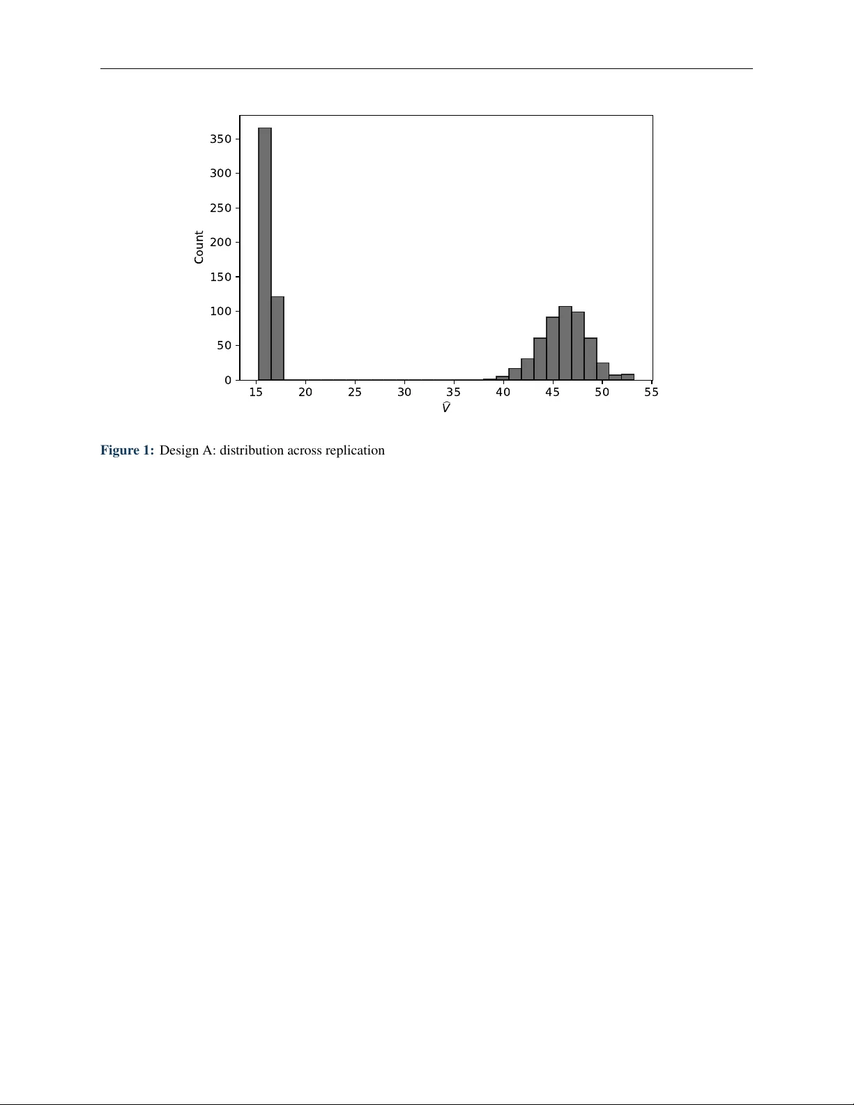
Fix ed-Horizon Self-N ormalized Inf erence f or A dap tiv e Experiments via Marting ale AIPW/DML with Logg ed Propensities Gabriel Saco U niver sidad del P acíﬁco OR CID : 0009-0009-8751-4154 Replica tion code : https:// github.com/gsaco/mar tingale- aipw- dml Abstract A daptive randomized experiments update treatment probabilities as data accrue, but still require an end-of-study interval f or the av erage treatment eﬀect (A TE) at a prespeciﬁed hor izon. U nder adaptiv e assignment, propensities can k eep changing, so the predictable quadratic variation of AIPW/DML score increments may remain random. When no deterministic v ar iance limit e xists, W ald statistics normalized b y a single long-r un v ar iance targ et can be conditionally miscalibrated given the realized v ar iance regime. W e assume no inter f erence, sequential randomization, i.i.d. ar r ivals, and e xecuted ov erlap on a prespeciﬁed scored set, and w e require two auditable pipeline conditions: the platf or m logs the e xecuted randomization probability f or each unit, and the nuisance regressions used to score unit 𝑡 are constructed predictably from pas t data only . These conditions make the centered AIPW/DML scores an e xact mar ting ale diﬀerence seq uence. Using self-normalized mar tingale limit theory , we show that the Studentized statistic, with variance estimated b y realized quadratic variation, is asymptotically N ( 0 , 1 ) at the prespeciﬁed horizon, e v en without v ar iance s tabilization. Simulations validate the theory and highlight when standard ﬁxed-v ar iance W ald repor ting f ails. 1 Gabriel Sa co Marting ale AIPW/DML Inf erence 1 Introduction A daptive randomized experiments—including response-adaptive clinical tr ials, contextual bandits, and larg e-scale platf or m experimentation sy stems—update assignment probabilities as data accr ue to balance learning and deployment ( Kasy and Sautmann , 2021 ). In practice, ho we ver , many platf orms still require con ventional end-of-study repor ting f or classical causal estimands such as the super population av erag e treatment eﬀect (A TE) computed once at a prespeciﬁed hor izon. Hereafter , w e denote b y 𝜋 𝑡 the ex ecuted assignment probability used to randomize unit 𝑡 after applying an y platform guardrails, as recorded in the e xper iment log. In this paper, we study ﬁx ed-hor izon W ald inference f or the standard logged-propensity AIPW/DML estimator , the sample av erag e of doubly robust pseudo-outcomes scored using these logged propensities. U nder adaptiv e assignment, the propensity process { 𝜋 𝑡 } is itself data-dependent, so the predictable quadratic variation of the AIPW/DML score increments can remain replication-random and need not conv erg e to a single deter ministic long-run v ariance targ et. Some end-of-study W ald arguments f or AIPW/A2IPW (and related DML estimators) under adaptivity proceed via Slutsky steps that rely on a deter ministic v ar iance targ et f or the predictable quadratic variation, often enf orced through stabilization-type or design-stability conditions on assignment probabilities and/or a verag e conditional v ar iances ( Hadad et al. , 2021 ; Zhan et al. , 2021 ; Kato et al. , 2020 ; Cook et al. , 2024 ; Li and Ow en , 2024 ; Sengupta et al. , 2025 ). On modern platf or ms, ho w ev er , the policy can keep reacting to noisy intermediate estimates. Clipping and guardrails can activate intermittently and batch updates can induce regime switches. When this happens, a W ald statis tic normalized using a single deter ministic v ar iance targ et can be systematicall y miscalibrated conditional on the realized variance regime, ev en if marginal co verag e appears close to nominal. W e treat the adaptiv e assignment policy as giv en but assume that the platform logs the e x ecuted propensity used to randomize each unit and that nuisance regressions used for AIPW/DML scoring are ﬁt predictably using only past data. Related w ork emphasizes that careful use of the logging policy and past-only ﬁtting is central for post-adaptiv e inf erence ( Bibaut et al. , 2021 ; Kato et al. , 2021 ; Cook et al. , 2024 ). U nder these auditable conditions, the centered score increments f or m an ex act mar tingale diﬀerence sequence, and we obtain ﬁxed-horizon W ald inf erence by studentizing with realized quadratic variation along the realized propensity path. This yields asymptotic N ( 0 , 1 ) calibration without requiring the predictable quadratic v ar iation to con ver ge to a deterministic long-r un variance target. 1 Contributions. • A udit able martingale scoring. W e formalize a logging/predictability contract, logged ex ecuted propensities and predictable nuisance ﬁtting, under which centered AIPW/DML score increments f orm an e xact mar tingale diﬀerence sequence (Lemma 5.3 ). • Fix ed-horizon self-normalized W ald inf erence. W e prov e that the usual Studentized statistic, with v ar iance estimated by realized quadratic v ar iation, is asymptoticall y N ( 0 , 1 ) at a prespeciﬁed hor izon e ven when no deter ministic long-r un variance limit e xists (Theorem 5.14 ). 1 W e do not claim an ytime-valid or optional-s topping guarantees. 2 Gabriel Sa co Marting ale AIPW/DML Inf erence • F easible studentization. W e sho w that the standard plug-in studentizer used in practice consistentl y estimates realized quadratic variation, so the f easible W ald inter val inher its the same ﬁxed-horizon v alidity (Proposition 4.11 ). • Oracle benchmar king and nuisance-learning eﬀects. W e pro vide a conditional second-moment decomposition yielding an oracle precision benchmark and isolate a nonnegativ e augmentation term capturing variance inﬂation from nuisance er ror (Proposition 5.8 ). Under w eighted 𝐿 2 con ver gence, the f easible statis tic is asymptoticall y oracle-equiv alent (Theorem C.4 ). The subsequent sections are structured as f ollo w s. Section 2 revie ws related w ork. Section 3 states the model and assumptions. Section 4 presents the estimator and auditable implementation details. Section 5 de velops the main theoretical results and Section 6 repor ts simulations. The appendices collect suppor ting limit-theory back g round, additional results and proofs, and an operational logging protocol. 2 R elated W ork Inf erence after adaptiv e dat a collection A growing literature studies inf erence with adaptivel y collected data, where obser vations are g enerated under an e vol ving inf or mation set and classical i.i.d. arguments do not directly appl y . Ear ly econometric w ork by Hahn et al. ( 2011 ) highlighted ho w propensity inf or mation can be le v eraged f or inf erence in sequential designs. More recent general frame works der iv e asymptotic representations f or seq uential decisions and adaptive e xper iments under broad conditions ( Hirano and P or ter , 2023 ). In the contextual-bandit and adaptiv e-e xper iment literature, ﬁx ed-hor izon inference has also been dev eloped via batc hed OLS/batchwise studentization arguments ( Zhang et al. , 2020 ). Our focus is narrow er but operationally central f or experimentation platf or ms: ﬁxed-horizon A TE reporting with logg ed e xecuted propensities and predictable AIPW/DML scor ing. In par ticular , w e tar g et settings where the predictable quadratic variation remains random across replications, so that deter ministic- v ariance nor malizations can be conditionally miscalibrated. General back g round on response-adaptiv e randomization and bandit-sty le designs can be f ound in Rosenber ger and Lachin ( 2015 ) and Villar et al. ( 2015 ). Stabilization, adaptiv e weighting and batching In adaptiv e e xper imentation and oﬀ-policy ev aluation, e v olving propensities can create hea vy tails and regime-dependent uncer tainty , motivating variance-control strategies. In policy ev aluation, Hadad et al. ( 2021 ) and Zhan et al. ( 2021 ) de velop adaptiv e weighting schemes f or augmented IPW/DR scores to obtain asymptoticall y nor mal 𝑡 -statis tics. For post-conte xtual-bandit inf erence, Bibaut et al. ( 2021 ) proposes stabilized doubly robust constructions that estimate conditional scale components using only past data. Another route restricts the data-collection design—f or e xample through batching—to reco v er classical CL T s f or bandit estimators ( Zhang et al. , 2020 ). In contras t, w e keep the standard logg ed-propensity AIPW/DML estimator unchang ed and do not require batching or adaptiv e re weighting. Instead, w e rely on a mar tingale score representation and studentization b y realized quadratic variation. 3 Gabriel Sa co Marting ale AIPW/DML Inf erence Design stability and deterministic variance-limit CL T s A fur ther line of work derives ﬁx ed-hor izon CL T s f or IPW/AIPW -type A TE estimators under e xplicit design stability conditions ensur ing that inv erse-propensity av erages and/or av erage conditional variances con v erg e to nonrandom limits, yielding con ventional deterministic asymptotic v ar iances f or W ald reporting ( Sengupta et al. , 2025 ). R elated perspectives arise when one engineers assignment r ules (or batchwise designs) to targ et eﬃciency or precision f or A2IPW/DML -sty le estimators ( Kato et al. , 2020 ; Li and Ow en , 2024 ; Cook et al. , 2024 ). More generall y , the adaptiv e-experiment literature emphasizes subtleties around what “the logging policy” means operationally when platforms implement clipping, guardrails, or algorithmic randomness ( Kato et al. , 2021 ). Our contribution is complementar y: w e assume the ex ecuted propensity actuall y used to randomize each unit is logged and we a v oid requiring con v erg ence of the predictable quadratic v ariation to a deterministic limit b y using realized quadratic variation as the nor malizer . Self-normalized martingale theory f or quadratic-v ariation studentization Our ﬁxed-horizon W ald statistic is a self-normalized mar tingale functional. Classic ref erences f or mar tingale CL T s and self-nor malized processes include Hall and He yde ( 1980 ) and de la P eña et al. ( 2009 ), as well as the surve y Shao and W ang ( 2013 ). Modern probability theor y pro vides reﬁned asymptotic and nonasymptotic control f or self-nor malized mar tingales, including Ber r y–Esseen bounds ( F an and Shao , 2017 ), Cramér -type moderate deviations ( F an et al. , 2019 ), and concentration inequalities ( Bercu and T ouati , 2019 ). W e appl y this theor y to AIPW/DML score increments under adaptive assignment, using realized quadratic variation to obtain a ﬁxed-horizon N ( 0 , 1 ) approximation without a deter ministic variance limit. An ytime-valid and time-unif orm alternatives The results in this paper are prespeciﬁed-hor izon and do not pro vide optional-stopping guarantees. When inf erence must remain valid under continuous monitor ing or data-dependent stopping, time-uniform methods based on test supermar tingales and conﬁdence sequences are appropr iate ( Ho ward et al. , 2021 ; W audb y -Smith et al. , 2024 ). R elated time-unif or m tools also appear alongside ﬁx ed-time inf erence in adaptiv e-e xper iment w ork ( Cook et al. , 2024 ; Kato et al. , 2020 ; W audby -Smith and Ramdas , 2023 ). W e f ocus ins tead on con ventional ﬁx ed-hor izon repor ting with realized quadratic-v ar iation studentization (see Remark 5.16 f or additional discussion). 3 Model and Assumptions 3.1 Propensities and Logged Assignment Rule Consider a stream of e xperimental units inde xed b y 𝑡 = 1 , . . . , 𝑛 . For eac h unit, cov ariates 𝑋 𝑡 are obser v ed bef ore assignment. The platform computes an assignment probability 𝜋 𝑡 ∈ ( 0 , 1 ) . Then, randomizes 𝐴 𝑡 ∈ { 0 , 1 } using 𝜋 𝑡 . Finall y , obser v es an outcome 𝑌 𝑡 . W e obser v e and store 𝑍 𝑡 : = ( 𝑋 𝑡 , 𝐴 𝑡 , 𝑌 𝑡 , 𝜋 𝑡 ) in time order . Let F 𝑡 : = 𝜎 ( 𝑍 1 , . . . , 𝑍 𝑡 ) , F 0 = { ∅ , Ω } , (3.1) 4 Gabriel Sa co Marting ale AIPW/DML Inf erence be the data ﬁltration. Let G 𝑡 : = 𝜎 ( F 𝑡 − 1 , 𝑋 𝑡 , 𝜋 𝑡 ) (3.2) be the 𝜎 -ﬁeld immediately bef ore randomization at time 𝑡 , after the platf or m has computed the e xecuted assignment probability 𝜋 𝑡 . The policy may be arbitrar il y adaptiv e or randomized. The ﬁx ed-hor izon v alidity results belo w require onl y that the realized e xecuted propensity used to randomize 𝐴 𝑡 is recorded in the log (Assumption 3.2 ). Deﬁnition 3.1 (A daptive logged ex ecuted propensity) . A t time 𝑡 , after observing ( F 𝑡 − 1 , 𝑋 𝑡 ) and an y algorithmic randomness used to f or m the propensity , the platf or m records the e xecuted assignment probability 𝜋 𝑡 ∈ ( 0 , 1 ) and dra ws treatment according to 𝐴 𝑡 | G 𝑡 ∼ Ber noulli ( 𝜋 𝑡 ) , where G 𝑡 is the pre-treatment 𝜎 -ﬁeld in ( 3.2 ) . If 𝜋 𝑡 is deter ministic giv en ( F 𝑡 − 1 , 𝑋 𝑡 ) , then 𝜋 𝑡 = P ( 𝐴 𝑡 = 1 | F 𝑡 − 1 , 𝑋 𝑡 ) . If 𝜋 𝑡 is produced using additional ex ogenous randomness, then P ( 𝐴 𝑡 = 1 | F 𝑡 − 1 , 𝑋 𝑡 ) = E [ 𝜋 𝑡 | F 𝑡 − 1 , 𝑋 𝑡 ] while still P ( 𝐴 𝑡 = 1 | G 𝑡 ) = 𝜋 𝑡 . W e treat any such platform-side randomness as ex ogenous, i.e., independent of ( 𝑌 𝑡 ( 0 ) , 𝑌 𝑡 ( 1 ) ) conditional on ( F 𝑡 − 1 , 𝑋 𝑡 ) . Assump tion 3.2 (Logging integr ity) . For each 𝑡 , the logg ed propensity 𝜋 𝑡 is G 𝑡 -measurable, takes values in ( 0 , 1 ) , and equals the probability passed to the randomization device that generated 𝐴 𝑡 , i.e., P ( 𝐴 𝑡 = 1 | G 𝑡 ) = 𝜋 𝑡 a.s. Equiv alently , 𝐴 𝑡 | G 𝑡 ∼ Ber noulli ( 𝜋 𝑡 ) with the logg ed 𝜋 𝑡 . 3.2 A udit diagnostics and data contract Remar k 3.3 (Auditing logg ed propensities) . Assumption 3.2 requires that, conditional on the platf or m history G 𝑡 (including the logged probability 𝜋 𝑡 ), the treatment assignment satisﬁes 𝐴 𝑡 | G 𝑡 ∼ Bernoulli ( 𝜋 𝑡 ) . This is a design-stag e proper ty . It holds only if the log records the probability that was actuall y passed to the randomization device. A basic diagnostic is calibration of 𝐴 𝑡 agains t 𝜋 𝑡 . For an y bin 𝐵 ⊂ ( 0 , 1 ) with many observations, let 𝑁 𝐵 : = 𝑛  𝑡 = 1 1 { 𝜋 𝑡 ∈ 𝐵 } , 𝐴 𝐵 : = 1 𝑁 𝐵  𝑡 : 𝜋 𝑡 ∈ 𝐵 𝐴 𝑡 , 𝜋 𝐵 : = 1 𝑁 𝐵  𝑡 : 𝜋 𝑡 ∈ 𝐵 𝜋 𝑡 . In practice, restrict attention to bins with 𝑁 𝐵 ≥ 𝑁 min f or a user -chosen 𝑁 min ≥ 1 (or merg e empty/small bins). U nder cor rect logging, 𝐴 𝐵 should be close to 𝜋 𝐵 up to mar tingale sampling variability ; under adaptivity , dependence can matter , so f or mal testing can be based on martingale concentration/self-nor malized methods f or the MDS ( 𝐴 𝑡 − 𝜋 𝑡 ) . These chec ks can detect se vere mis-logging or implementation bugs, but the y cannot cer tify cor rect logging or validate the causal assumptions in Assumptions 3.5 – 3.7 . Remar k 3.4 (Timing and measurability) . The experiment unf olds in the order (1) obser v e 𝑋 𝑡 ; (2) the platf or m computes and logs an e xecuted propensity 𝜋 𝑡 as a function of ( F 𝑡 − 1 , 𝑋 𝑡 ) ; (3) treatment is dra wn according to 𝐴 𝑡 | G 𝑡 ∼ Ber noulli ( 𝜋 𝑡 ) ; and (4) the outcome 𝑌 𝑡 is rev ealed and logged. In par ticular, 𝜋 𝑡 is G 𝑡 -measurable, 5 Gabriel Sa co Marting ale AIPW/DML Inf erence while ( 𝐴 𝑡 , 𝑌 𝑡 ) are F 𝑡 -measurable. This timing underlies the predictability requirement in Section 4 and the data-contract protocol in Appendix E . Step Object Measurability / check 1 Observe cov ar iates 𝑋 𝑡 observed at 𝑡 (pre-treatment) 2 Choose/log 𝜋 𝑡 𝜋 𝑡 must be G 𝑡 -measurable; log the e xecuted random-number generator (RNG) probability 3 Randomize 𝐴 𝑡 𝐴 𝑡 | G 𝑡 ∼ Ber noulli ( 𝜋 𝑡 ) (Assumption 3.2 ) 4 Observe outcome 𝑌 𝑡 realized after 𝐴 𝑡 5 Fit/update nuisances f or 𝑡 + 1 nuisance used at 𝑡 + 1 must be F 𝑡 -measurable T able 1: Timing and measurability . The key analytical requirement is that the nuisance used to score unit 𝑡 is F 𝑡 − 1 -measurable (Assumption 4.5 ). Symbol Meaning 𝑛 , 𝑡 ﬁx ed hor izon; unit index 𝑡 = 1 , . . . , 𝑛 𝑍 𝑡 logged record ( 𝑋 𝑡 , 𝐴 𝑡 , 𝑌 𝑡 , 𝜋 𝑡 ) F 𝑡 , G 𝑡 post-outcome history; pre-treatment info ( 3.1 )–( 3.2 ) 𝜋 𝑡 logged e xecuted propensity ; P ( 𝐴 𝑡 = 1 | G 𝑡 ) = 𝜋 𝑡 (Ass. 3.2 ) 𝑌 𝑡 ( 𝑎 ) , 𝑌 𝑡 potential outcomes; obser ved 𝑌 𝑡 = 𝐴 𝑡 𝑌 𝑡 ( 1 ) + ( 1 − 𝐴 𝑡 ) 𝑌 𝑡 ( 0 ) 𝑚 ★ 𝑎 true regression 𝑥 ↦→ E [ 𝑌 ( 𝑎 ) | 𝑋 = 𝑥 ] b 𝑚 𝑡 − 1 , 𝑎 predictable nuisance used at time 𝑡 (Ass. 4.5 ) 𝜙 𝑡 ( 𝑚 , 𝜋 ) AIPW/DR pseudo-outcome ev aluated at propensity 𝜋 ( 4.1 ) b 𝜙 𝑡 , b 𝜃 scored pseudo-outcome b 𝜙 𝑡 = 𝜙 𝑡 ( b 𝑚 𝑡 − 1 , 𝜋 𝑡 ) and estimator ( 4.3 ) 𝜃 0 , b 𝜃 A TE ( 3.3 ); estimator ( 4.3 ) 𝜉 𝑡 , 𝑆 T increment 𝜉 𝑡 = b 𝜙 𝑡 − 𝜃 0 ; sum 𝑆 T = Í 𝑡 ∈ T 𝜉 𝑡 T , 𝑛 eﬀ scored inde x set; 𝑛 eﬀ : = | T | 𝑄 T , 𝑉 2 T , b 𝑉 realized/predictable QV ( 5.3 ); studentizer ( 4.4 ) T able 2: Summar y of notation. 3.3 P otential Outcomes and T arget Parameter W e adopt the potential outcomes frame w ork with the usual no interference and consistency con ventions. Assump tion 3.5 (Consistency and no inter ference; SUTV A) . For each unit 𝑡 , there are well-deﬁned potential outcomes ( 𝑌 𝑡 ( 0 ) , 𝑌 𝑡 ( 1 ) ) that depend onl y on the assignment of unit 𝑡 itself (see R ubin , 1980 ). The obser v ed outcome satisﬁes 𝑌 𝑡 = 𝑌 𝑡 ( 𝐴 𝑡 ) = 𝐴 𝑡 𝑌 𝑡 ( 1 ) + ( 1 − 𝐴 𝑡 ) 𝑌 𝑡 ( 0 ) a.s. The targ et parameter is the a verag e treatment eﬀect (A TE) in the super population: 𝜃 0 : = E  𝑌 ( 1 ) − 𝑌 ( 0 )  , (3.3) where ( 𝑋 , 𝑌 ( 0 ) , 𝑌 ( 1 ) ) denotes a g ener ic dra w from the superpopulation descr ibed in Assumption 3.6 . Assumption 3.5 is standard. It r ules out spillov ers or network eﬀects, which require separate methods. 6 Gabriel Sa co Marting ale AIPW/DML Inf erence 3.4 Assump tions W e maintain the f ollo wing assumptions throughout. Assump tion 3.6 (Superpopulation ar r iv als; no selection) . The sequence { ( 𝑋 𝑡 , 𝑌 𝑡 ( 0 ) , 𝑌 𝑡 ( 1 ) ) } 𝑛 𝑡 = 1 is independent across 𝑡 and identically distributed with generic draw ( 𝑋 , 𝑌 ( 0 ) , 𝑌 ( 1 ) ) . In par ticular , the adaptiv e policy aﬀects only treatment assignment, not which units/co variates ar r iv e. W e wr ite all e xpectations with respect to this super population draw , so 𝜃 0 = E [ 𝑌 ( 1 ) − 𝑌 ( 0 ) ] and 𝜏 ( 𝑥 ) : = E [ 𝑌 ( 1 ) − 𝑌 ( 0 ) | 𝑋 = 𝑥 ] satisfy 𝜃 0 = E [ 𝜏 ( 𝑋 ) ] . As noted in Remark 5.7 , the proof s only require the conditional mean-stationarity condition E [ 𝜏 ( 𝑋 𝑡 ) | F 𝑡 − 1 ] = 𝜃 0 . Assump tion 3.7 (Sequential randomization/no anticipation) . 𝐴 𝑡 ⊥ ⊥ ( 𝑌 𝑡 ( 0 ) , 𝑌 𝑡 ( 1 ) ) | G 𝑡 , where G 𝑡 is the pre-treatment 𝜎 -ﬁeld in ( 3.2 ) . Equiv alently , conditional on the pre-treatment inf ormation (including the realized e x ecuted propensity 𝜋 𝑡 ), the treatment dra w is independent of the potential outcomes. Assump tion 3.8 (Ex ecuted o v erlap on scored units) . There exis ts 𝜀 > 0 such that f or ev ery time inde x whose score is included in the ﬁnal estimator (i.e., 𝑡 ∈ T in Section 4 ), 𝜀 ≤ 𝜋 𝑡 ≤ 1 − 𝜀 a.s. (3.4) A suﬃcient operational mechanism is to enforce clipping of the e xecuted propensity before randomization on all scored units. Assump tion 3.9 (Moment conditions) . For eac h 𝑎 ∈ { 0 , 1 } , E [ | 𝑌 ( 𝑎 ) | 4 ] < ∞ . Assump tion 3.10 (Nuisance stability) . There e xists a ﬁnite constant 𝐶 < ∞ such that f or each 𝑎 ∈ { 0 , 1 } , sup 𝑛 ≥ 1 sup 𝑡 ∈ T E [ | b 𝑚 𝑡 − 1 , 𝑎 ( 𝑋 𝑡 ) | 4 ] ≤ 𝐶 . In unbounded-outcome settings, a suﬃcient alternative is to tr uncate/clamp b 𝑚 𝑡 − 1 , 𝑎 ( 𝑋 𝑡 ) at a larg e threshold; see Remark 3.11 . Remar k 3.11 (Ho w to enf orce Assumption 3.10) . If outcomes are kno wn to be bounded, say 𝑌 𝑡 ∈ [ − 𝐵 , 𝐵 ] , w e can enf orce Assumption 3.10 by clipping b 𝑚 𝑡 − 1 , 𝑎 ( 𝑥 ) to [ − 𝐵 , 𝐵 ] (or slightly wider) f or each 𝑎 . For unbounded outcomes, one ma y instead tr uncate at a larg e threshold or use robust regression; this is a technical de vice to control moments and does not chang e the target estimand. Remar k 3.12 (W eaker moment conditions are possible but are not needed f or this paper) . Self-nor malized mar ting ale CL T s only require ﬁnite ( 2 + 𝛿 ) moments of the score increments. W e impose f our th moments to keep the quadratic-v ar iation equivalence proof fully transparent. Remar k 3.13 (Design-stag e, analy sis-stag e and auditable conditions) . Our validity results combine (i) substantiv e causal/model assumptions and (ii) pipeline conditions that can be check ed from logs and stored ar tif acts. 1. Substantiv e assumptions. SUTV A/no inter f erence (Assumption 3.5 ) and sequential randomization with a stable targ et estimand (Assumption 3.7 ), tog ether with i.i.d. ar r iv als/no selection (Assumption 3.6 ) or an e xplicit mean-stationarity alter nativ e (R emark 5.7 ). 7 Gabriel Sa co Marting ale AIPW/DML Inf erence 2. Auditable design-time requir ements. Logg ed ex ecuted propensities (Assumption 3.2 ) and e xecuted o v erlap on the scored units (Assumption 3.8 ), which must be enf orced at assignment time if needed (e.g., b y clipping 𝜋 𝑡 ). 3. Auditable analysis-time r equirements. A prespeciﬁed (deterministic) scored set T (Assumption 4.8 ) and predictable nuisance constr uction (Assumption 4.5 ), which rule out “peeking” when ﬁtting the regressions used to score each unit. 4. Regularity conditions. Moment and stability bounds (Assumptions 3.9 and 3.10 ) and variance growth (Assumption 5.11 ) needed to apply mar ting ale limit theor y . Finall y , all conﬁdence intervals are ﬁx ed-horizon: they should be repor ted only at the prespeciﬁed sample size and are g enerall y inv alid under optional stopping (R emark 5.16 and Appendix E ). 4 Predictable AIPW/DML Estimation 4.1 The Doubly Robust Score Let 𝑚 ★ 𝑎 ( 𝑥 ) : = E [ 𝑌 ( 𝑎 ) | 𝑋 = 𝑥 ] and write 𝑚 ★ : = ( 𝑚 ★ 0 , 𝑚 ★ 1 ) . F or an y candidate 𝑚 = ( 𝑚 0 , 𝑚 1 ) and an y 𝜋 ∈ ( 0 , 1 ) , deﬁne the usual augmented inv erse-propensity weighted (AIPW) / doubly robust (DR) score ( R obins et al. , 1994 ; Bang and Robins , 2005 ) (pseudo-outcome) 𝜙 𝑡 ( 𝑚 , 𝜋 ) : = 𝐴 𝑡 𝜋  𝑌 𝑡 − 𝑚 1 ( 𝑋 𝑡 )  − 1 − 𝐴 𝑡 1 − 𝜋  𝑌 𝑡 − 𝑚 0 ( 𝑋 𝑡 )  + 𝑚 1 ( 𝑋 𝑡 ) − 𝑚 0 ( 𝑋 𝑡 ) . (4.1) When ev aluating at the logged e xecuted propensity , w e wr ite 𝜙 𝑡 ( 𝑚 ) : = 𝜙 𝑡 ( 𝑚 , 𝜋 𝑡 ) f or brevity . The quantity 𝜙 𝑡 ( 𝑚 , 𝜋 𝑡 ) is obser vable giv en ( 𝑋 𝑡 , 𝐴 𝑡 , 𝑌 𝑡 , 𝜋 𝑡 ) and a supplied regression pair 𝑚 . For the oracle regression 𝑚 ★ , one can decompose 𝜙 𝑡 ( 𝑚 ★ ) = 𝜏 ( 𝑋 𝑡 ) + 𝐴 𝑡 𝜋 𝑡  𝑌 𝑡 ( 1 ) − 𝑚 ★ 1 ( 𝑋 𝑡 )  − 1 − 𝐴 𝑡 1 − 𝜋 𝑡  𝑌 𝑡 ( 0 ) − 𝑚 ★ 0 ( 𝑋 𝑡 )  . (4.2) The centered increment 𝜙 𝑡 ( 𝑚 ★ ) − 𝜃 0 has mean zero and is the object gov er ned by the mar tingale CL T . Remar k 4.1 (T er minology) . The estimating function 𝜙 𝑡 ( 𝑚 , 𝜋 𝑡 ) in ( 4.1 ) has the classical doubly robust/AIPW f or m. When e valuated at the tr ue reg ression functions 𝑚 ★ (and the e xecuted propensities), the centered score 𝜙 𝑡 ( 𝑚 ★ , 𝜋 𝑡 ) − 𝜃 0 coincides with the eﬃcient inﬂuence function f or the A TE in the cor responding i.i.d. model with kno wn propensity (see, e.g., Hahn ( 1998 ); T siatis ( 2006 )). For g eneral 𝑚 , it is simpl y an estimating function with the same doubl y robust f or m. In oﬀ-policy ev aluation and conte xtual-bandit settings, essentially the same form appears as a doubly robust score f or v alue estimation ( Dudik et al. , 2011 , 2014 ). Remar k 4.2 (Multi-ar m extensions) . The results e xtend directl y to 𝐾 > 2 arms by replacing the scalar propensity with a probability v ector and using the cor responding multivariate AIPW score. For simplicity , we present the binar y case. 8 Gabriel Sa co Marting ale AIPW/DML Inf erence 4.2 F orwar d Cross-Fitting Standard cross-ﬁtting par titions data into f olds and estimates nuisances on held-out f olds. Under adaptivity , w e must respect time: nuisance estimates used at time 𝑡 must be constructed from data str ictl y bef ore 𝑡 . Deﬁnition 4.3 (Forward cross-ﬁtting) . Par tition indices { 1 , . . . , 𝑛 } into 𝐾 contiguous blocks 𝐼 1 , . . . , 𝐼 𝐾 . The par tition is deter ministic and ﬁxed prior to data collection. F or each bloc k 𝑘 ≥ 2 : 1. Estimate nuisance functions ( b 𝑚 ( − 𝑘 ) 0 , b 𝑚 ( − 𝑘 ) 1 ) using only data from blocks 𝐼 1 , . . . , 𝐼 𝑘 − 1 . 2. For eac h 𝑡 ∈ 𝐼 𝑘 , ev aluate the score using these estimates and the logged propensity 𝜋 𝑡 . For 𝑡 ∈ 𝐼 1 , use a pilot estimate or ex clude 𝐼 1 from inf erence. Remar k 4.4 (Common pitf all) . A common pitfall is to use i.i.d.-sty le sample splitting or cross-ﬁtting patter ns that inadvertently allo w information from unit 𝑡 (or future units) to enter the nuisance reg ression used to score unit 𝑡 . In adaptive e xper iments, such “leakage ” violates Assumption 4.5 and can break the mar tingale diﬀerence property in Lemma 5.3 . As a result, the Studentized W ald statis tic built from leaky scores g enerally lacks the ﬁx ed-hor izon guarantee of Theorem 5.14 : it may still w ork in some ﬁnite-sample designs, but its v alidity is no long er ensured by the martingale argument. Appendix E giv es an auditable implementation pattern (f or w ard cross-ﬁtting) that enf orces predictability . Assump tion 4.5 (Predictable nuisance constr uction) . F or each scored time 𝑡 ∈ T and treatment arm 𝑎 ∈ { 0 , 1 } , the regression function b 𝑚 𝑡 − 1 , 𝑎 used in the score for unit 𝑡 is F 𝑡 − 1 -measurable. Equiv alently , conditional on the past F 𝑡 − 1 , the function b 𝑚 𝑡 − 1 , 𝑎 does not depend on ( 𝐴 𝑡 , 𝑌 𝑡 ) or on an y future data. Assumption 4.5 is the f or mal predictability requirement (“no-peeking”, i.e., no use of contemporaneous or future outcomes) that makes the scored pseudo-outcomes a mar tingale diﬀerence sequence, and predictable ﬁts are not based on non-predictable (“leaky”) scores (see Lemma 4.6 below). The measurability here ref ers to the ﬁtted function object b 𝑚 𝑡 − 1 , 𝑎 ; it may then be ev aluated at the cur rent cov ariate 𝑋 𝑡 to f or m b 𝑚 𝑡 − 1 , 𝑎 ( 𝑋 𝑡 ) . It r ules out i.i.d.-sty le cross-ﬁtting schemes that, ev en indirectly , use contemporaneous or future outcomes when constructing the nuisance for time 𝑡 . A simple wa y to enf orce predictability is f or w ard cross-ﬁtting (Deﬁnition 4.3 ): par tition the time axis into blocks 𝐼 1 , . . . , 𝐼 𝐾 , ﬁt each nuisance model once per block using onl y data from ∪ 𝑗 < 𝑘 𝐼 𝑗 , and hold the ﬁtted model ﬁxed while scor ing units in 𝐼 𝑘 . T o make this requirement auditable, an implementation should persist (i) the training indices used for eac h ﬁt, (ii) fold assignments if internal cross-v alidation is used, and (iii) all learner randomness. Lemma 4.6 (A suﬃcient operational condition for predictability) . U nder f or war d cross-ﬁtting (Deﬁnition 4.3 ), if for eac h block 𝐼 𝑘 the analys t ﬁts ( b 𝑚 ( − 𝑘 ) 0 , b 𝑚 ( − 𝑘 ) 1 ) using only data fr om bloc ks 𝐼 1 , . . . , 𝐼 𝑘 − 1 and then reuses these ﬁtted objects unchang ed for all 𝑡 ∈ 𝐼 𝑘 , then Assumption 4.5 holds. Pr oof. For 𝑡 ∈ 𝐼 𝑘 , the ﬁtted objects depend onl y on 𝜎 ( 𝑍 𝑠 : 𝑠 ∈ 𝐼 1 ∪ · · · ∪ 𝐼 𝑘 − 1 ) ⊆ F 𝑡 − 1 and are therefore F 𝑡 − 1 -measurable. Remar k 4.7 (Connection to A2IPW ter minology) . Our b 𝜙 𝑡 is the same AIPW/DR pseudo-outcome used in the adaptiv e-e xperiment literature under the name A2IPW (adaptive AIPW). A t time 𝑡 the score is computed using outcome reg ressions ﬁtted on past data onl y , together with the logg ed e xecuted propensity used to randomize 𝐴 𝑡 ( Kato et al. , 2020 ; Cook et al. , 2024 ). The present paper emphasizes that this predictability requirement is 9 Gabriel Sa co Marting ale AIPW/DML Inf erence not merely a conv enience: it is the condition that yields an e xact mar tingale diﬀerence sequence and enables ﬁx ed-hor izon Studentized inf erence without any stabilization of propensities or conditional variances. 4.3 The Estimator Let T ⊆ { 1 , . . . , 𝑛 } denote the set of indices f or which the nuisance used at time 𝑡 is predictable (i.e., b 𝑚 𝑡 − 1 is F 𝑡 − 1 -measurable). U nder f or ward cross-ﬁtting with a bur n-in block 𝐼 1 , one typically takes T : = { 1 , . . . , 𝑛 } \ 𝐼 1 . Let 𝑛 eﬀ : = Í 𝑛 𝑡 = 1 1 { 𝑡 ∈ T } = | T | . Throughout the asymptotic theor y we treat the scored index set T as deterministic, as is the case under the forw ard-block construction in Deﬁnition 4.3 . Assump tion 4.8 (Deter ministic scored set) . The scored inde x set T ⊆ { 1 , . . . , 𝑛 } is ﬁx ed pr ior to data collection (equiv alentl y , 𝑇 𝑡 : = 1 { 𝑡 ∈ T } is nonrandom f or each 𝑡 ). Remar k 4.9 (Predictable scored sets) . If 𝑇 𝑡 : = 1 { 𝑡 ∈ T } is allo wed to be F 𝑡 − 1 -measurable, the same proof strategy applies to ˜ 𝜉 𝑡 : = 𝑇 𝑡 ( b 𝜙 𝑡 − 𝜃 0 ) . In this case, inter pret 𝑛 eﬀ : = Í 𝑛 𝑡 = 1 𝑇 𝑡 and deﬁne 𝑄 T and 𝑉 2 T using ˜ 𝜉 𝑡 . W e omit fur ther details of the predictable- T e xtension to keep the note f ocused. Estimator and studentizing factor . The cross-ﬁtted pseudo-outcome is b 𝜙 𝑡 : = 𝜙 𝑡 ( b 𝑚 𝑡 − 1 , 𝜋 𝑡 ) , b 𝜃 : = 1 𝑛 eﬀ  𝑡 ∈ T b 𝜙 𝑡 . (4.3) where b 𝑚 𝑡 − 1 is the predictable nuisance estimate. b 𝑉 : = 1 𝑛 eﬀ − 1  𝑡 ∈ T ( b 𝜙 𝑡 − b 𝜃 ) 2 , deﬁned f or 𝑛 eﬀ ≥ 2 . (4.4) Remar k 4.10 (The studentizer as realized quadratic v ar iation) . Let 𝑛 eﬀ : = | T | and recall b 𝑉 in ( 4.4 ) and 𝑄 T in ( 5.3 ). A direct calculation giv es ( 𝑛 eﬀ − 1 ) b 𝑉 = 𝑄 T − 𝑛 eﬀ ( b 𝜃 − 𝜃 0 ) 2 . (4.5) Thus b 𝑉 is essentiall y the realized quadratic variation 𝑄 T up to the negligible center ing term 𝑛 eﬀ ( b 𝜃 − 𝜃 0 ) 2 / ( 𝑛 eﬀ − 1 ) . Proposition 4.11 records a minimal condition under which ( 𝑛 eﬀ − 1 ) b 𝑉 / 𝑄 T → 𝑝 1 . Proposition 4.11 (Feasibility of the studentizer) . Let 𝜉 𝑡 : = b 𝜙 𝑡 − 𝜃 0 and 𝑆 T : = Í 𝑡 ∈ T 𝜉 𝑡 , so that b 𝜃 − 𝜃 0 = 𝑆 T / 𝑛 eﬀ and 𝑄 T = Í 𝑡 ∈ T 𝜉 2 𝑡 . If 𝑛 eﬀ → ∞ and 𝑆 T / √ 𝑄 T = 𝑂 𝑝 ( 1 ) , then ( 𝑛 eﬀ − 1 ) b 𝑉 𝑄 T → 𝑝 1 . In particular , the condition 𝑆 T / √ 𝑄 T = 𝑂 𝑝 ( 1 ) holds whenev er 𝑆 T / √ 𝑄 T ⇒ N ( 0 , 1 ) . Pr oof. By ( 4.5 ), ( 𝑛 eﬀ − 1 ) b 𝑉 𝑄 T = 1 − 1 𝑛 eﬀ  𝑆 T √ 𝑄 T  2 , which con ver ges to 1 in probability under the stated conditions. 10 Gabriel Sa co Marting ale AIPW/DML Inf erence Score sum notation. Deﬁne the centered increments 𝜉 𝑡 : = b 𝜙 𝑡 − 𝜃 0 and the score sum 𝑆 T : = Í 𝑡 ∈ T 𝜉 𝑡 = 𝑛 eﬀ ( b 𝜃 − 𝜃 0 ) . c SE : =  b 𝑉 / 𝑛 eﬀ . (4.6) CI 1 − 𝛼 = h b 𝜃 ± 𝑧 1 − 𝛼 / 2 c SE i . (4.7) Remar k 4.12 (Finite- 𝑛 repor ting conv ention) . For small 𝑛 eﬀ , it is common as a pragmatic ﬁnite-sample con vention to also repor t a 𝑡 -critical v ariant using 𝑡 0 . 975 , 𝑛 eﬀ − 1 , namely 𝐶 𝐼 𝑡 : = b 𝜃 ± 𝑡 0 . 975 , 𝑛 eﬀ − 1  b 𝑉 / 𝑛 eﬀ , where b 𝑉 is the sample variance in ( 4.4 ) . This is a repor ting con v ention; we do not claim ﬁnite-sample Student- 𝑡 v alidity , and it is not co v ered b y Theorem 5.14 . 5 Main Theoretical Results Remar k 5.1 (T r iangular -ar ra y and uniformity con vention) . All objects may depend on the horizon 𝑛 (e.g. f or w ard blocks and nuisance ﬁts). W e suppress the inde x 𝑛 and assume ov erlap and moment constants are unif or m o ver 𝑛 . This section isolates the logic behind predictable AIPW/DML in adaptive experiments. First, under logg ed e xecuted propensities and predictable nuisance ﬁts, the centered score is an e xact martingale diﬀerence, yielding ﬁnite-sample conditional unbiasedness (Proposition 5.2 and Lemma 5.3 ). Second, ﬁxed-horizon inf erence f ollow s from a self-normalized mar tingale CL T applied to the mar tingale sum, with f easibility pro vided b y a sample-v ar iance appro ximation (Theorem 5.14 ). T able 10 in Appendix D maps each assumption to each statement, and Appendix A states the mar tingale limit theorem inv oked in the proofs. 5.1 The Martingale Structure The central insight of our anal ysis is that f orward cross-ﬁtting induces a mar tingale diﬀerence structure. W e ﬁrst establish an identiﬁcation result f or the pseudo-outcome. Proposition 5.2 (Identiﬁcation, including predictable random nuisances) . Let 𝑚 𝑡 − 1 = ( 𝑚 𝑡 − 1 , 0 , 𝑚 𝑡 − 1 , 1 ) be any (possibly r andom) pair of r egr ession functions that is F 𝑡 − 1 -measur able. Under Assumptions 3.6 , 3.2 , and 3.7 , for eac h 𝑡 , E  𝜙 𝑡 ( 𝑚 𝑡 − 1 ) | G 𝑡  = 𝜏 ( 𝑋 𝑡 ) . (5.1) Consequently , E [ 𝜙 𝑡 ( 𝑚 𝑡 − 1 ) ] = 𝜃 0 . Pr oof. Fix 𝑡 and condition on G 𝑡 = 𝜎 ( F 𝑡 − 1 , 𝑋 𝑡 , 𝜋 𝑡 ) . Since 𝑚 𝑡 − 1 is F 𝑡 − 1 -measurable and F 𝑡 − 1 ⊆ G 𝑡 , the function 𝑚 𝑡 − 1 is ﬁxed under this conditioning. By sequential randomization (Assumption 3.7 ), E [ 𝑌 𝑡 | G 𝑡 , 𝐴 𝑡 = 1 ] = E [ 𝑌 𝑡 ( 1 ) | G 𝑡 ] , E [ 𝑌 𝑡 | G 𝑡 , 𝐴 𝑡 = 0 ] = E [ 𝑌 𝑡 ( 0 ) | G 𝑡 ] . By i.i.d. ar r ivals (Assumption 3.6 ) and the e x ogeneity condition in Deﬁnition 3.1 , ( 𝑌 𝑡 ( 0 ) , 𝑌 𝑡 ( 1 ) ) ⊥ ⊥ ( F 𝑡 − 1 , 𝜋 𝑡 ) | 𝑋 𝑡 and thus E [ 𝑌 𝑡 ( 𝑎 ) | 𝑋 𝑡 , F 𝑡 − 1 , 𝜋 𝑡 ] = E [ 𝑌 𝑡 ( 𝑎 ) | 𝑋 𝑡 ] = 𝑚 ★ 𝑎 ( 𝑋 𝑡 ) f or 𝑎 ∈ { 0 , 1 } . 11 Gabriel Sa co Marting ale AIPW/DML Inf erence Using E [ 𝐴 𝑡 | G 𝑡 ] = 𝜋 𝑡 and the tow er proper ty , E  𝐴 𝑡 ( 𝑌 𝑡 − 𝑚 𝑡 − 1 , 1 ( 𝑋 𝑡 ) ) 𝜋 𝑡    G 𝑡  = E  𝐴 𝑡 𝜋 𝑡 E [ 𝑌 𝑡 − 𝑚 𝑡 − 1 , 1 ( 𝑋 𝑡 ) | G 𝑡 , 𝐴 𝑡 ]    G 𝑡  = E  𝐴 𝑡 𝜋 𝑡 ( 𝑚 ★ 1 ( 𝑋 𝑡 ) − 𝑚 𝑡 − 1 , 1 ( 𝑋 𝑡 ) )    G 𝑡  = 𝑚 ★ 1 ( 𝑋 𝑡 ) − 𝑚 𝑡 − 1 , 1 ( 𝑋 𝑡 ) , and similarl y E  ( 1 − 𝐴 𝑡 ) ( 𝑌 𝑡 − 𝑚 𝑡 − 1 , 0 ( 𝑋 𝑡 ) ) 1 − 𝜋 𝑡    G 𝑡  = 𝑚 ★ 0 ( 𝑋 𝑡 ) − 𝑚 𝑡 − 1 , 0 ( 𝑋 𝑡 ) . Plugging into the deﬁnition of 𝜙 𝑡 ( 𝑚 𝑡 − 1 ) in ( 4.1 ) yields E [ 𝜙 𝑡 ( 𝑚 𝑡 − 1 ) | G 𝑡 ] = ( 𝑚 𝑡 − 1 , 1 ( 𝑋 𝑡 ) − 𝑚 𝑡 − 1 , 0 ( 𝑋 𝑡 ) ) + ( 𝑚 ★ 1 ( 𝑋 𝑡 ) − 𝑚 𝑡 − 1 , 1 ( 𝑋 𝑡 ) ) − ( 𝑚 ★ 0 ( 𝑋 𝑡 ) − 𝑚 𝑡 − 1 , 0 ( 𝑋 𝑡 ) ) = 𝑚 ★ 1 ( 𝑋 𝑡 ) − 𝑚 ★ 0 ( 𝑋 𝑡 ) = 𝜏 ( 𝑋 𝑡 ) , which pro v es ( 5.1 ). T aking unconditional e xpectations gives E [ 𝜙 𝑡 ( 𝑚 𝑡 − 1 ) ] = E [ 𝜏 ( 𝑋 𝑡 ) ] = 𝜃 0 . The k ey consequence is that the pseudo-outcome, when e valuated with any predictable nuisance estimates, remains conditionally unbiased. Lemma 5.3 (Mar tingale diﬀerence structure) . Suppose Assumptions 3.6 , 3.2 , 3.7 , 3.9 , and 3.10 hold. Let { b 𝑚 𝑡 − 1 } satisfy Assumption 4.5 . F or each scor ed index 𝑡 ∈ T , deﬁne b 𝜙 𝑡 : = 𝜙 𝑡 ( b 𝑚 𝑡 − 1 ) and 𝜉 𝑡 : = b 𝜙 𝑡 − 𝜃 0 . Then E [ b 𝜙 𝑡 | F 𝑡 − 1 ] = 𝜃 0 , (5.2) and { 𝜉 𝑡 , F 𝑡 } is a marting ale diﬀer ence sequence o ver the scor ed indices. Pr oof. (A ﬁnite ﬁrst moment suﬃces here; this f ollo ws from Assumption 3.9 . Higher -moment bounds used later are provided b y Lemma 5.6 .) Using iterated e xpectations and Proposition 5.2 , E [ 𝜙 𝑡 ( b 𝑚 𝑡 − 1 ) | F 𝑡 − 1 ] = E  E [ 𝜙 𝑡 ( b 𝑚 𝑡 − 1 ) | G 𝑡 ] | F 𝑡 − 1  = E [ 𝜏 ( 𝑋 𝑡 ) | F 𝑡 − 1 ] . By Assumption 3.6 , 𝑋 𝑡 is independent of F 𝑡 − 1 , so E [ 𝜏 ( 𝑋 𝑡 ) | F 𝑡 − 1 ] = E [ 𝜏 ( 𝑋 ) ] = 𝜃 0 . Corollary 5.4 (Finite-sample unbiasedness) . Under Assumptions 3.6 , 3.2 , 3.7 , 4.8 , 3.9 , 3.10 , and pr edictable nuisances as in Assumption 4.5 , we hav e E [ b 𝜃 ] = 𝜃 0 . Pr oof. By linearity and Lemma 5.3 , E [ b 𝜃 ] = 1 𝑛 eﬀ  𝑡 ∈ T E [ 𝜙 𝑡 ( b 𝑚 𝑡 − 1 ) ] = 1 𝑛 eﬀ  𝑡 ∈ T 𝜃 0 = 𝜃 0 . 12 Gabriel Sa co Marting ale AIPW/DML Inf erence Remar k 5.5 (Inter pretation) . Lemma 5.3 is the conceptual replacement f or f old-wise independence in i.i.d. DML. Rather than requiring approximate independence betw een nuisance estimation and score ev aluation, w e e xploit ex act conditional unbiasedness given the past. This mar tingale s tr ucture holds f or any quality of nuisance estimates, pro vided the y are predictable. Lemma 5.6 (Moment bounds) . Suppose Assumptions 3.9 , 3.10 , and 3.8 hold. Then ther e exists a constant 𝐶 < ∞ such that sup 𝑛 ≥ 1 sup 𝑡 ∈ T E  | b 𝜙 𝑡 | 4  ≤ 𝐶 . Pr oof. Fix 𝑡 ∈ T . By o v erlap, 𝜋 𝑡 ∈ [ 𝜀 , 1 − 𝜀 ] almost surel y , so the inv erse-propensity w eights are unif or mly bounded on scored indices. Appl ying ( 𝑎 + 𝑏 + 𝑐 + 𝑑 ) 4 ≤ 4 3 ( 𝑎 4 + 𝑏 4 + 𝑐 4 + 𝑑 4 ) to the score f ormula ( 4.1 ) (and hence to ( 4.3 )) and using Assumptions 3.9 and 3.10 yields the claimed uniform bound. Remar k 5.7 (W eaker than i.i.d.) . Lemma 5.3 uses Assumption 3.6 only through the implication E [ 𝜏 ( 𝑋 𝑡 ) | F 𝑡 − 1 ] = 𝜃 0 . Thus the MDS argument e xtends to any ar r ival process satisfying this mean-s tationar ity condition. 5.2 The V ariance Structure Bef ore stating the CL T , we analyze the variance structure. Deﬁne the realized and predictable quadratic v ar iations: 𝑄 T : =  𝑡 ∈ T 𝜉 2 𝑡 , 𝑉 2 T : =  𝑡 ∈ T E [ 𝜉 2 𝑡 | F 𝑡 − 1 ] . (5.3) Proposition 5.8 (Conditional second-moment decomposition and oracle benchmark) . Suppose Assump- tions 3.6 , 3.2 , and 3.7 hold. Le t 𝜎 2 𝑎 ( 𝑋 𝑡 ) : = V ar ( 𝑌 𝑡 ( 𝑎 ) | 𝑋 𝑡 ) and deﬁne the reg ression bias terms 𝑏 𝑎 ( 𝑥 ) : = 𝑚 𝑎 ( 𝑥 ) − 𝑚 ★ 𝑎 ( 𝑥 ) . Then f or each 𝑡 ∈ T , E [ ( 𝜙 𝑡 ( 𝑚 ) − 𝜃 0 ) 2 | G 𝑡 ] = ( 𝜏 ( 𝑋 𝑡 ) − 𝜃 0 ) 2 + 𝜎 2 1 ( 𝑋 𝑡 ) 𝜋 𝑡 + 𝜎 2 0 ( 𝑋 𝑡 ) 1 − 𝜋 𝑡 + 𝜋 𝑡 ( 1 − 𝜋 𝑡 )  𝑏 1 ( 𝑋 𝑡 ) 𝜋 𝑡 + 𝑏 0 ( 𝑋 𝑡 ) 1 − 𝜋 𝑡  2 . (5.4) Mor eov er , since E [ 𝜙 𝑡 ( 𝑚 ) | G 𝑡 ] = 𝜏 ( 𝑋 𝑡 ) f or any 𝑚 that is F 𝑡 − 1 -measur able, the last thr ee terms in ( 5.4 ) equal V ar ( 𝜙 𝑡 ( 𝑚 ) | G 𝑡 ) . In par ticular , relativ e to the oracle scor e 𝜙 𝑡 ( 𝑚 ★ ) (f or whic h 𝑏 0 = 𝑏 1 ≡ 0 ), using a misspeciﬁed 𝑚 adds a nonneg ative augmentation term to the conditional second moment and conditional v ariance. Pr oof. Deﬁne 𝜀 𝑡 , 𝑎 : = 𝑌 𝑡 ( 𝑎 ) − 𝑚 ★ 𝑎 ( 𝑋 𝑡 ) , so that E [ 𝜀 𝑡 , 𝑎 | 𝑋 𝑡 ] = 0 and E [ 𝜀 2 𝑡 , 𝑎 | 𝑋 𝑡 ] = 𝜎 2 𝑎 ( 𝑋 𝑡 ) . A direct e xpansion using sequential randomization yields 𝜙 𝑡 ( 𝑚 ) − 𝜏 ( 𝑋 𝑡 ) = 𝐴 𝑡 𝜋 𝑡 𝜀 𝑡 , 1 − 1 − 𝐴 𝑡 1 − 𝜋 𝑡 𝜀 𝑡 , 0 − 𝐴 𝑡 − 𝜋 𝑡 𝜋 𝑡 𝑏 1 ( 𝑋 𝑡 ) − 𝐴 𝑡 − 𝜋 𝑡 1 − 𝜋 𝑡 𝑏 0 ( 𝑋 𝑡 ) , from which ( 5.4 ) f ollo ws b y taking conditional second moments giv en G 𝑡 and adding ( 𝜏 ( 𝑋 𝑡 ) − 𝜃 0 ) 2 . Finall y , since E [ 𝜙 𝑡 ( 𝑚 ) | G 𝑡 ] = 𝜏 ( 𝑋 𝑡 ) f or any 𝑚 that is F 𝑡 − 1 -measurable (in par ticular , an y predictable learner), the last three ter ms in ( 5.4 ) are all centered at the oracle benchmark 𝜏 ( 𝑋 𝑡 ) , and the proof is complete. Remar k 5.9 (Oracle case and variance inﬂation are immediate) . Setting 𝑚 = 𝑚 ★ in Proposition 5.8 remo ves the nonnegativ e augmentation ter m and yields the oracle conditional second moment. The f actors 1 / 𝜋 𝑡 and 13 Gabriel Sa co Marting ale AIPW/DML Inf erence 1 / ( 1 − 𝜋 𝑡 ) make e xplicit how e xtreme propensities inﬂate uncer tainty , motivating o v erlap enf orcement at the design stag e. Remar k 5.10 (Wh y learn 𝑚 without rates?) . Theorem 5.14 yields v alid prespeciﬁed-hor izon co verag e under predictability and logged propensities without requiring that b 𝑚 𝑡 − 1 , 𝑎 con ver ges to 𝑚 ★ 𝑎 at any particular rate. Learning 𝑚 is theref ore not needed f or v alidity; it is needed f or precision. Proposition 5.8 show s that the oracle score 𝜙 𝑡 ( 𝑚 ★ ) remo ves a nonnegativ e augmentation ter m from the conditional second moment, providing a natural benchmark f or how nuisance quality aﬀects the size of the studentizer . The oracle reg ression 𝑚 ★ minimizes the conditional v ar iance within the AIPW score f amily (Proposition 5.8 ), and the augmentation term shrinks as 𝑚 approaches 𝑚 ★ . This does not imply monotone tightening relativ e to an arbitrar y baseline across lear ning iterations. There is no monotonic guarantee relativ e to an arbitrary baseline. A poorl y chosen nuisance can increase or decrease v ar iance compared to another misspeciﬁed choice. 5.3 Studentized Asymp totic Normality W e no w state our main inf erential result. The k ey ingredient is that the realized quadratic variation 𝑄 T and its predictable counter par t 𝑉 2 T are asymptotically equiv alent under mild conditions, enabling studentization with the f easible sample variance b 𝑉 . R oadmap. Lemma 5.3 identiﬁes the scored sum 𝑆 T as a martingale sum with predictable quadratic variation 𝑉 2 T and realized quadratic v ariation 𝑄 T ; Assumption 4.8 ensures that the scored indicator 1 { 𝑡 ∈ T } is deterministic (hence predictable). T o apply the self-normalized mar tingale CL T in Theorem A.1 , w e v er ify : (i) 𝑉 2 T → ∞ (Assumption 5.11 ); (ii) 𝑄 T / 𝑉 2 T → 𝑝 1 via a standard martingale variance-ratio argument, using the unif or m f our th-moment bound from Lemma 5.6 ; and (iii) a L yapuno v condition, again by Lemma 5.6 together with Assumption 5.11 . Finall y , Proposition 4.11 justiﬁes replacing 𝑄 T b y ( 𝑛 eﬀ − 1 ) b 𝑉 in the Studentized statis tic. Assump tion 5.11 (V ar iance gro wth / nondegeneracy) . As 𝑛 → ∞ , 𝑛 eﬀ : = | T | → ∞ and there e xists 𝑣 − > 0 such that P  𝑉 2 T ≥ 𝑣 − 𝑛 eﬀ  → 1 . This is a nondeg eneracy lo wer bound ensuring the predictable quadratic variation g ro ws at least linearl y in 𝑛 eﬀ ; it does not impose v ar iance stabilization. A simple pr imitiv e suﬃcient condition for Assumption 5.11 is that outcome noise is nondeg enerate and o v erlap holds under the standing causal/sequential assumptions of Section 3 . The f ollo wing corollar y records a suﬃcient condition; see Appendix C.3 f or the proof. Corollary 5.12 (A suﬃcient condition f or v ar iance gro wth) . Suppose Assumptions 3.6 , 3.2 , 3.7 , 3.8 , and C.6 hold, where Assumption C.6 (Appendix) is the nondeg ener acy condition E [ 𝜎 2 1 ( 𝑋 ) + 𝜎 2 0 ( 𝑋 ) ] ≥ 𝜎 2 > 0 . Then Assumption 5.11 holds. Remar k 5.13 (Nondegeneracy and numerical guardrails) . Assumption 5.11 implies the quadratic variation gro ws, so b 𝑉 is bounded a wa y from zero with high probability asymptotically . In ﬁnite samples, if b 𝑉 = 0 (e.g. constant outcomes), inf erence is uninf or mativ e; repor t this as a design/measurement degeneracy . 14 Gabriel Sa co Marting ale AIPW/DML Inf erence Theorem 5.14 (Studentized ﬁx ed-hor izon inf erence without v ar iance s tabilization) . Suppose Assumptions 3.6 , 3.2 , 3.7 , 3.8 , 4.5 , 4.8 , 3.9 , 3.10 , and 5.11 hold. Let 𝑛 eﬀ : = | T | and recall 𝑆 T = Í 𝑡 ∈ T ( b 𝜙 𝑡 − 𝜃 0 ) and 𝑄 T = Í 𝑡 ∈ T ( b 𝜙 𝑡 − 𝜃 0 ) 2 . Then 𝑆 T √ 𝑄 T ⇒ N ( 0 , 1 ) , (5.5) and the practical Studentized statis tic satisﬁes √ 𝑛 eﬀ ( b 𝜃 − 𝜃 0 ) b 𝑉 1 / 2 ⇒ N ( 0 , 1 ) , (5.6) wher e b 𝑉 is deﬁned in ( 4.4 ) . Consequently , the W ald interval ( 4.7 ) has asymptotically correct cov erag e at the pr especiﬁed horizon, without req uiring v ariance stabilization (i.e., 𝑉 2 T / 𝑛 eﬀ → 𝑉 det er ministic; Assumption C.1 ). Pr oof. Let 𝜉 𝑡 : = 1 { 𝑡 ∈ T } ( b 𝜙 𝑡 − 𝜃 0 ) and 𝑆 T : = Í 𝑡 ∈ T 𝜉 𝑡 . U nder Assumptions 3.6 , 3.2 , 3.7 , 4.5 , and 4.8 , Lemma 5.3 implies that ( 𝜉 𝑡 , F 𝑡 ) is a mar tingale diﬀerence ar ray . Assumption 5.11 giv es 𝑉 2 T : = Í 𝑡 ∈ T E [ 𝜉 2 𝑡 | F 𝑡 − 1 ] → ∞ . Lemma 5.6 (which uses Assumptions 3.9 , 3.10 , and 3.8 ) pro vides a unif orm fourth-moment bound f or the scored increments; together with Assumption 5.11 , a standard mar tingale v ar iance-ratio calculation (see Appendix B ) v er iﬁes the v ar iance-ratio and L yapuno v conditions required by Theorem A.1 . Theref ore Theorem A.1 yields 𝑆 T / √ 𝑄 T ⇒ N ( 0 , 1 ) , i.e., ( 5.5 ) . Finall y , Proposition 4.11 implies ( 𝑛 eﬀ − 1 ) b 𝑉 / 𝑄 T → 𝑝 1 , and Slutsky’ s theorem yields ( 5.6 ). Remar k 5.15 (V alidity vs. precision and consistency) . The studentized CL T in Theorem 5.14 does not require b 𝑚 𝑡 − 1 to conv erg e to 𝑚 ★ f or v alidity . Predictability (Assumption 4.5 ) together with o v erlap and moment/stability conditions (Assumptions 3.8 – 3.10 ) and v ariance gro wth (Assumption 5.11 ) are suﬃcient. N uisance learning is nonetheless valuable: b y Proposition 5.8 the oracle reg ression 𝑚 ★ minimizes the conditional v ariance within the AIPW score f amily (Proposition 5.8 ), and the augmentation ter m shr inks as 𝑚 approaches 𝑚 ★ ; this does not imply monotone tightening relative to an arbitrar y baseline across learning iterations. In par ticular , b 𝜃 is consistent whene ver 𝑛 eﬀ → ∞ , and b 𝑉 is a f easible studentizer e ven when 𝑉 2 T / 𝑛 eﬀ does not stabilize. Remar k 5.16 (R elation to stabilization-based and an ytime-valid approac hes) . Some ﬁx ed-hor izon CL T s in the adaptiv e-e xperiment literature nor malize by a deter ministic asymptotic variance, imposing stabilization/design- stability conditions ensuring that an av erage conditional variance (or , equivalentl y , 𝑉 2 T / 𝑛 eﬀ ) conv erg es to a deterministic limit ( Hadad et al. , 2021 ; Zhan et al. , 2021 ; Kato et al. , 2021 ; Cook et al. , 2024 ; Sengupta et al. , 2025 ; Zenati et al. , 2025 ). Such assumptions are appropr iate when the deplo y ed policy stabilizes or when one e xplicitly engineers stability . Theorem 5.14 takes a diﬀerent route. W e normalize b y the realized quadratic variation, so validity does not require a deter ministic variance limit. This directly accommodates regimes where propensities oscillate, conv erge to random limits, or other wise f ail to stabilize, while still deliv er ing a conv entional ﬁx ed-hor izon W ald inter v al. F inall y , Theorem 5.14 is a prespeciﬁed-hor izon result. If the e xper iment is continuousl y monitored and potentially stopped earl y based on the data, time-uniform methods such as conﬁdence sequences and time-unif or m CL T s are needed ( Ho ward et al. , 2021 ; W audby -Smith and Ramdas , 15 Gabriel Sa co Marting ale AIPW/DML Inf erence 2023 ; W audby -Smith et al. , 2024 ). Because our score increments f or m an ex act MDS, the setup is compatible with standard time-unif or m mar tingale methods, but w e do not dev elop anytime-v alid inference here. Appendix C collects three extensions not needed f or the main methods-note claim: (i) a non-studentized CL T under variance stabilization; (ii) oracle equiv alence under 𝐿 2 nuisance consistency ; and (iii) a pr imitiv e suﬃcient condition for v ar iance g ro wth. 6 Simulation Study W e compare ﬁx ed-hor izon 95% W ald inter vals of the f or m ( 4.7 ) under diﬀerent nor malizations and nuisance- ﬁtting regimes, depending on the design: (CI1) SN (self-normalized): the proposed studentized W ald interval ( 4.7 ). (CI2) Fix ed- 𝑉 (stabilization-style baseline): a W ald inter val that replaces the (potentially random) long-r un v ar iance b y a ﬁx ed constant 𝑉 ﬁx , b 𝜃 ± 𝑧 1 − 𝛼 / 2  𝑉 ﬁx / 𝑛 eﬀ , thereb y beha ving as if Assumption C.1 held with deterministic limit. W e specify 𝑉 ﬁx e xplicitly in each design. (CI3) Leaky baselines (Designs C1 and D): nuisance ﬁts that violate predictability (Assumption 4.5 ) by using contemporaneous or future outcomes when scor ing unit 𝑡 . When computed, the score is still ( 4.1 ) and the CI is ( 4.7 ), but the ﬁx ed-hor izon guarantee of Theorem 5.14 does not appl y . (CI4) Regime-a war e Fixed- 𝑉 (Design A only): an inf easible regime-aw are ﬁxed-v ar iance benchmark that plugs in the cor rect regime-speciﬁc 𝑉 ﬁx based on the burn-in sign. For each design w e repor t: (i) tw o-sided 95% cov erage; (ii) a verag e CI length; and (iii) where inf or mativ e, mean bias and/or null rejection rates. Monte Carlo standard er rors f or cov erage are (  ˆ 𝑝 ( 1 − ˆ 𝑝 ) / 𝑅 ) . T ables repor t 𝑛 and 𝑛 eﬀ e xplicitly . Unless noted, w e use 𝑅 = 1000 replications and 𝑛 ∈ { 250 , 500 , 1000 , 2000 , 5000 } . 6.1 Design A: random long-run variance During burn-in, 𝜋 𝑡 = 0 . 5 f or 𝑡 ≤ 𝑛 0 = 50 , and w e compute the bur n-in estimate b 𝜏 burn : = 1 𝑛 0 𝑛 0  𝑡 = 1  𝐴 𝑡 𝑌 𝑡 𝜋 𝑡 − ( 1 − 𝐴 𝑡 ) 𝑌 𝑡 1 − 𝜋 𝑡  using only bur n-in units. After burn-in, if b 𝜏 burn ≥ 0 then 𝜋 𝑡 = 0 . 8 , else 𝜋 𝑡 = 0 . 2 . Outcomes: 𝑌 ( 0 ) ∼ N ( 0 , 1 ) and 𝑌 ( 1 ) = 𝜀 1 with 𝜀 1 ∼ N ( 0 , 9 ) . There are no co variates; with 𝑚 0 ≡ 𝑚 1 ≡ 0 , the AIPW score ( 4.1 ) reduces to the usual in verse-propensity w eighted (IPW) score. On T = { 𝑛 0 + 1 , . . . , 𝑛 } w e ha ve 𝑛 eﬀ = 𝑛 − 𝑛 0 and 𝜋 𝑡 is constant after bur n-in, so the oracle conditional v ar iance con v erg es to a random limit: 𝑉 2 T 𝑛 eﬀ →        9 / 0 . 8 + 1 / 0 . 2 = 16 . 25 , b 𝜏 burn ≥ 0 , 9 / 0 . 2 + 1 / 0 . 8 = 46 . 25 , b 𝜏 burn < 0 . 16 Gabriel Sa co Marting ale AIPW/DML Inf erence Thus Assumption C.1 fails (no deterministic variance limit). The SN CI remains valid under Theorem 5.14 because it self-nor malizes by realized quadratic variation. SN uses ( 4.7 ) . Fix ed- 𝑉 sets 𝑉 ﬁx : = 31 . 25 (the unconditional mean of the two v ar iance limits abo ve). R egime-aw are Fix ed- 𝑉 plugs in 𝑉 ﬁx = 16 . 25 or 46 . 25 depending on the realized bur n-in sign. T able 3: Design A: co v erage and length of 95% CIs. 𝑛 𝑛 eﬀ Method Co verag e MCSE A vg. length 250 200 Fix ed- V 0.944 (0.007) 1.549 250 200 Regime-F ixed 0.950 (0.007) 1.515 250 200 SN 0.955 (0.007) 1.506 500 450 Fix ed- V 0.939 (0.008) 1.033 500 450 Regime-F ixed 0.950 (0.007) 1.003 500 450 SN 0.957 (0.006) 1.002 1000 950 Fix ed- V 0.938 (0.008) 0.711 1000 950 Regime-F ixed 0.948 (0.007) 0.697 1000 950 SN 0.948 (0.007) 0.696 2000 1950 Fix ed- V 0.947 (0.007) 0.496 2000 1950 Regime-F ixed 0.941 (0.007) 0.477 2000 1950 SN 0.946 (0.007) 0.476 5000 4950 Fix ed- V 0.941 (0.007) 0.311 5000 4950 Regime-F ixed 0.960 (0.006) 0.303 5000 4950 SN 0.959 (0.006) 0.303 Notes: 𝑅 = 1000 replications; 𝑛 ∈ { 250 , 500 , 1000 , 2000 , 5000 } ; burn-in 𝑛 0 = 50 (so 𝑛 eﬀ = 𝑛 − 50 ). SN is the studentized inter val ( 4.7 ) . F ixed- 𝑉 uses 𝑉 ﬁx = 31 . 25 , the unconditional mean of the regime-speciﬁc variance limits. Regime-a ware Fixed- 𝑉 is an infeasible oracle benc hmark that plugs in the cor rect regime-speciﬁc variance ter m (i.e., 𝜎 2 1 = 9 and 𝜎 2 0 = 1 , so the regime-speciﬁc limits are 9 / 0 . 8 + 1 / 0 . 2 = 16 . 25 and 9 / 0 . 2 + 1 / 0 . 8 = 46 . 25 ), and uses 𝑧 -cr itical values. T able 3 repor ts marginal co v erage and a v erag e length f or Design A as 𝑛 increases. In this design, the studentized SN inter val remains close to the nominal 95% le vel across hor izons, consistent with Theorem 5.14 . The ﬁxed- 𝑉 interval nor malizes by a single deter ministic targ et 𝑉 that av erages o ver the two pos t–burn-in propensity regimes. As a consequence, its marginal cov erage can be close to nominal while still e xhibiting regime-dependent ov er/under co v erage (T able 4 ). The regime-a ware ﬁx ed- 𝑉 benchmark, which plugs in the cor rect regime-speciﬁc variance constant, illustrates that classical normalization w orks once one conditions on (and cor rectly accounts for) the realized variance regime. The SN inter v al achiev es this conditioning automaticall y via studentization. Design A illustrates the basic phenomenon targ eted b y Theorem 5.14 : the v ar iance pro xy 𝑉 2 T / 𝑛 eﬀ does not con ver ge to a single deterministic constant because it depends on the realized post–burn-in propensity regime. T able 4 sho ws that a ﬁxed- 𝑉 normalization can be conser vativ e when the realized regime has lo w variance ( 𝜋 𝑡 = 0 . 8 ) and anti-conser vativ e when the realized regime has high variance ( 𝜋 𝑡 = 0 . 2 ). In contrast, the SN interval studentizes b y the realized quadratic variation and maintains near -nominal conditional co verag e in both regimes. 17 Gabriel Sa co Marting ale AIPW/DML Inf erence Method P ost burn-in 𝜋 𝑛 = 250 𝑛 = 500 𝑛 = 1000 𝑛 = 2000 SN 0 . 8 0.96 0.97 0.95 0.95 SN 0 . 2 0.95 0.95 0.94 0.94 Fix ed- 𝑉 0 . 8 1.00 0.99 0.99 1.00 Fix ed- 𝑉 0 . 2 0.89 0.89 0.89 0.89 Notes: Each ro w conditions on the realized post–bur n-in propensity in Design A: if b 𝜏 burn ≥ 0 then 𝜋 𝑡 = 0 . 8 f or ( 𝑡 > 𝑛 0 ) , and if b 𝜏 burn < 0 then 𝜋 𝑡 = 0 . 2 for ( 𝑡 > 𝑛 0 ) . T able 4: Conditional co verag e b y realized propensity regime (Design A) 6.2 Design B: stabilization benchmar k Design B provides a benchmark setting in which the conditional variance stabilizes. W e adopt the outcome model from Design A with 𝜏 = 0 , 𝑌 ( 0 ) ∼ N ( 0 , 1 ) , and 𝑌 ( 1 ) = 𝜀 1 where 𝜀 1 ∼ N ( 0 , 9 ) . T reatment is assigned with a constant ex ecuted propensity 𝜋 𝑡 ≡ 0 . 6 f or all 𝑡 ≤ 𝑛 , so there is no burn-in and 𝑛 eﬀ = 𝑛 . Because there are no cov ar iates, the AIPW score coincides with the IPW score. In this setting, Assumption C.1 holds with a deterministic long-r un variance, 𝑉 ﬁx = 9 0 . 6 + 1 0 . 4 = 17 . 5 , and theref ore the SN and Fix ed- 𝑉 intervals are asymptotically equiv alent. T able 5: Design B (s tabilization benchmark): co verag e and length of 95% CIs. 𝑛 𝑛 eﬀ Method Co verag e MCSE A v g. length 250 250 Fix ed- V 0.954 (0.007) 1.037 250 250 SN 0.952 (0.007) 1.038 500 500 Fix ed- V 0.949 (0.007) 0.733 500 500 SN 0.953 (0.007) 0.733 1000 1000 Fix ed- V 0.957 (0.006) 0.519 1000 1000 SN 0.955 (0.007) 0.518 2000 2000 Fix ed- V 0.953 (0.007) 0.367 2000 2000 SN 0.953 (0.007) 0.366 5000 5000 Fix ed- V 0.947 (0.007) 0.232 5000 5000 SN 0.947 (0.007) 0.232 Notes: 𝑅 = 1000 replications; 𝑛 ∈ { 250 , 500 , 1000 , 2000 , 5000 } ; 𝑛 eﬀ = 𝑛 . SN is ( 4.7 ). Fixed- 𝑉 uses 𝑉 ﬁx = 17 . 5 . T able 5 sho ws that when the variance stabilizes, SN and Fix ed- 𝑉 giv e nearl y identical co v erage and length. Diﬀerences are within Monte Carlo er ror , consistent with the deter ministic 𝑉 ﬁx . 6.3 Design C1: leakage stress test Design C1 is a stress test f or Assumption 4.5 and Remark 4.4 . Co variates are 𝑋 𝑡 ∈ R 𝑝 with 𝑝 = 20 and i.i.d. 𝑋 𝑡 ∼ N ( 0 , 𝐼 𝑝 ) . P otential outcomes f ollo w 𝑌 𝑡 ( 0 ) = 𝑚 0 ( 𝑋 𝑡 ) + 𝜀 𝑡 0 , 𝑌 𝑡 ( 1 ) = 𝑚 0 ( 𝑋 𝑡 ) + 𝜏 ( 𝑋 𝑡 ) + 𝜀 𝑡 1 , 18 Gabriel Sa co Marting ale AIPW/DML Inf erence where 𝑚 0 ( 𝑥 ) is nonlinear and 𝜏 ( 𝑥 ) = 𝜏 0 + 𝛿 sin ( 𝑥 1 ) so the superpopulation A TE equals 𝜃 0 = E [ 𝜏 ( 𝑋 𝑡 ) ] = 𝜏 0 . W e repor t calibration at 𝜏 0 = 0 with 𝛿 = 0 . 2 ; er rors are independent 𝑡 30 dra ws rescaled to unit v ar iance (ﬁnite moments, but heavier tails than Gaussian). T o induce adaptiv e feedbac k, w e split { 1 , . . . , 𝑛 } into 𝐾 = 5 contiguous blocks and use the ﬁrst block as burn-in with 𝜋 𝑡 ≡ 0 . 5 . On subsequent blocks, the e xecuted propensity is 𝜋 𝑡 = 𝜀 + ( 1 − 2 𝜀 ) e xpit  𝜆 b 𝜏 𝑡 − 1 ( 𝑋 𝑡 )  , b 𝜏 𝑡 − 1 ( 𝑥 ) = b 𝑚 𝑡 − 1 , 1 ( 𝑥 ) − b 𝑚 𝑡 − 1 , 0 ( 𝑥 ) , with 𝜀 = 0 . 1 and 𝜆 = 2 . 5 . The predictable nuisance b 𝑚 𝑡 − 1 , 𝑎 is ﬁt by ridge regression on a lo w-dimensional f eature map using only pr ior blocks and held ﬁx ed within the cur rent block (f or w ard ﬁtting). The leaky baseline ﬁts a richer r idge model once on the full sample, violating predictability . T able 6: Design C1 (predictability / leakag e stress test, 𝜏 0 = 0 ): cov erage, length, and null rejection. 𝑛 𝑛 eﬀ Method Co verag e MCSE A vg. length Reject rate 250 200 SN-AIPW -Predictable 0.952 (0.007) 0.653 0.048 250 200 SN-AIPW -LeakyFull 0.821 (0.012) 1.864 0.179 250 200 SN-IPW 0.939 (0.008) 0.766 0.061 500 400 SN-AIPW -Predictable 0.953 (0.007) 0.429 0.047 500 400 SN-AIPW -LeakyFull 0.887 (0.010) 0.398 0.113 500 400 SN-IPW 0.958 (0.006) 0.525 0.042 1000 800 SN-AIPW -Predictable 0.948 (0.007) 0.290 0.052 1000 800 SN-AIPW -LeakyFull 0.928 (0.008) 0.274 0.072 1000 800 SN-IPW 0.947 (0.007) 0.360 0.053 2000 1600 SN-AIPW -Predictable 0.957 (0.006) 0.202 0.043 2000 1600 SN-AIPW -LeakyFull 0.944 (0.007) 0.195 0.056 2000 1600 SN-IPW 0.962 (0.006) 0.251 0.038 5000 4000 SN-AIPW -Predictable 0.944 (0.007) 0.126 0.056 5000 4000 SN-AIPW -LeakyFull 0.941 (0.007) 0.124 0.059 5000 4000 SN-IPW 0.951 (0.007) 0.157 0.049 Notes: 𝑅 = 1000 replications; 𝐾 = 5 contiguous blocks with the ﬁrst block omitted from scoring (so 𝑛 eﬀ = 4 𝑛 / 5 ). The e xecuted propensity is 𝜋 𝑡 = 𝜀 + ( 1 − 2 𝜀 ) expit ( 𝜆 b 𝜏 𝑡 − 1 ( 𝑋 𝑡 ) ) with 𝜀 = 0 . 1 and 𝜆 = 2 . 5 . “SN-AIPW -Predictable” uses forward (past-only) r idge nuisances; “SN-AIPW -LeakyFull” ﬁts a full-sample r idge nuisance on r icher f eatures and is not predictable. Reject rate is the two-sided rejection probability of 𝐻 0 : 𝜃 0 = 0 based on the cor responding 95% CI. T able 6 makes the predictability requirement operational: the predictable SN- AIPW procedure remains near nominal, while the leaky full-sample nuisance substantiall y underco vers and ov er -rejects at smaller horizons, consistent with the warning in Remark 4.4 . 6.4 Design C2: nuisance quality Design C2 isolates ho w nuisance quality aﬀects precision without confounding from adaptivity . Cov ar iates 𝑋 𝑡 ∈ R 5 f ollo w a cor related nor mal with AR(1) cor relation 𝜌 = 0 . 5 ; treatment is assigned with constant propensity 𝜋 𝑡 ≡ 0 . 5 . Potential outcomes are linear with homoskedastic noise: 𝑌 𝑡 ( 0 ) = 𝑋 𝑡 1 + 𝑋 𝑡 2 + 𝜀 𝑡 0 , 𝑌 𝑡 ( 1 ) = 𝑋 𝑡 1 + 𝑋 𝑡 2 + 𝜏 + 𝜀 𝑡 1 , 𝜀 𝑡 0 , 𝜀 𝑡 1 i.i.d. ∼ N ( 0 , 1 ) , 19 Gabriel Sa co Marting ale AIPW/DML Inf erence so the oracle regression remov es the augmentation ter m in Proposition 5.8 . W e use 𝐾 = 10 f or w ard blocks (ﬁrst bloc k omitted) and repor t results at 𝑛 = 5000 under 𝜏 = 0 . T able 7: Design C2 (precision vs nuisance quality , 𝑛 = 5000 ): co verag e and relativ e length/variance v s oracle. 𝑛 𝑛 eﬀ Method Co verag e MCSE A vg. length Rel. length R el. b 𝑉 5000 4500 SN-AIPW -Oracle 0.955 (0.007) 0.117 1.000 1.000 5000 4500 SN-AIPW - W ellSpec 0.951 (0.007) 0.117 1.002 1.004 5000 4500 SN-AIPW -Misspec 0.956 (0.006) 0.155 1.323 1.750 5000 4500 SN-IPW 0.937 (0.008) 0.234 1.999 3.997 Notes: 𝑅 = 1000 replications; 𝜋 𝑡 ≡ 0 . 5 ; 𝐾 = 10 f or ward blocks with the ﬁrst block omitted from scor ing (so 𝑛 eﬀ = 4500 ). “W ellSpec” ﬁts arm-speciﬁc linear regression on all cov ar iates; “Misspec” ﬁts on a restricted co variate set; “SN-IPW” sets 𝑚 ≡ 0 . Relativ e quantities are computed with respect to the oracle procedure within the same design. T able 7 show s the oracle benc hmarking messag e: co v erage remains near nominal across nuisance choices, while interval length (and b 𝑉 ) inﬂates as the nuisance becomes more misspeciﬁed, consistent with Proposition 5.8 and the “validity vs precision ” discussion f ollowing Theorem 5.14 . 6.5 Design D: adaptiv e policy and logging integrity Design D is a simple conte xtual-bandit-sty le adaptive experiment that highlights the design-time role of e xecuted propensity logging (Assumption 3.2 ). Co v ar iates are 𝑋 𝑡 ∈ R 10 with correlated normal 𝑋 𝑡 ∼ N ( 0 , Σ ) where Σ 𝑖 𝑗 = 𝜌 | 𝑖 − 𝑗 | and 𝜌 = 0 . 3 . The baseline outcome, heterogeneous treatment eﬀect, and heteroskedas tic noise are 𝑚 0 ( 𝑥 ) = 0 . 8 𝑥 1 + 0 . 5 𝑥 2 2 − 0 . 5 cos ( 𝑥 3 ) + 0 . 25 𝑥 4 , 𝜏 ( 𝑥 ) = 0 . 5 𝑥 1 + 0 . 5 sin ( 𝑥 2 ) + 0 . 25 1 { 𝑥 3 > 0 } − 0 . 25 𝑥 4 𝑥 5 , 𝜎 ( 𝑥 ) = 1 + 0 . 5 | 𝑥 1 | , 𝑌 𝑡 ( 𝑎 ) = 𝑚 𝑎 ( 𝑋 𝑡 ) + 𝜀 𝑡 𝑎 , 𝜀 𝑡 𝑎 | 𝑋 𝑡 ∼ N ( 0 , 𝜎 ( 𝑋 𝑡 ) 2 ) , so 𝜃 0 = E [ 𝜏 ( 𝑋 𝑡 ) ] is the A TE. W e use bur n-in 𝑛 0 = 100 with 𝜋 𝑡 ≡ 0 . 5 and then update in blocks of size 100: on each block w e ﬁt ar m-speciﬁc linear regressions on past data only and choose the e xecuted propensity by either an 𝜀 -greedy rule or a softmax rule, clipping to [ 0 . 05 , 0 . 95 ] to enf orce o v erlap. W e compare: (i) SN-AIPW with predictable (past-onl y) nuisance ﬁts; (ii) Naiv e-iid-DML using leaky 5-f old cross-ﬁtting that ignores time ordering; (iii) SN-IPW with 𝑚 ≡ 0 ; (iv) SN-Oracle using the true 𝑚 0 , 𝑚 1 ; and (v) SN-IPW -Assume0p5, an analy sis-time mis-logging baseline that computes the score using 𝜋 𝑡 ≡ 0 . 5 rather than the logg ed e x ecuted propensity 𝜋 𝑡 . T ables 8 – 9 sho w tw o complementar y messages: with the logged e xecuted propensities and predictable nuisance ﬁtting, the studentized intervals are close to nominal under both adaptiv e policies; in contrast, the mis-logg ed “ Assume0p5” baseline is se verel y biased and has catastrophic underco v erage, illustrating wh y Assumption 3.2 is design-critical. 20 Gabriel Sa co Marting ale AIPW/DML Inf erence T able 8: Design D (adaptiv e assignment, 𝜀 -g reedy policy): co verag e, length, and bias of 95% CIs. 𝑛 𝑛 eﬀ Method Co verag e MCSE A vg. length Bias 250 150 SN-Oracle 0.946 (0.007) 1.516 0.009 250 150 SN-AIPW 0.944 (0.007) 1.906 0.019 250 150 Naiv e-iid-DML 0.944 (0.007) 1.883 0.019 250 150 SN-IPW 0.934 (0.008) 2.083 0.003 250 150 SN-IPW -Assume0p5 0.433 (0.016) 1.296 0.703 500 400 SN-Oracle 0.950 (0.007) 0.940 -0.008 500 400 SN-AIPW 0.939 (0.008) 1.174 -0.012 500 400 Naiv e-iid-DML 0.943 (0.007) 1.166 -0.014 500 400 SN-IPW 0.951 (0.007) 1.304 -0.017 500 400 SN-IPW -Assume0p5 0.064 (0.008) 0.795 0.869 1000 900 SN-Oracle 0.948 (0.007) 0.629 0.003 1000 900 SN-AIPW 0.954 (0.007) 0.784 -0.006 1000 900 Naiv e-iid-DML 0.950 (0.007) 0.786 -0.006 1000 900 SN-IPW 0.947 (0.007) 0.864 -0.003 1000 900 SN-IPW -Assume0p5 0.005 (0.002) 0.528 0.943 2000 1900 SN-Oracle 0.953 (0.007) 0.433 0.001 2000 1900 SN-AIPW 0.955 (0.007) 0.543 0.001 2000 1900 Naiv e-iid-DML 0.948 (0.007) 0.548 0.001 2000 1900 SN-IPW 0.952 (0.007) 0.596 -0.003 2000 1900 SN-IPW -Assume0p5 0.001 (0.001) 0.363 0.979 5000 4900 SN-Oracle 0.958 (0.006) 0.271 -0.001 5000 4900 SN-AIPW 0.955 (0.007) 0.342 0.000 5000 4900 Naiv e-iid-DML 0.954 (0.007) 0.347 0.001 5000 4900 SN-IPW 0.955 (0.007) 0.372 -0.002 5000 4900 SN-IPW -Assume0p5 0.003 (0.002) 0.226 0.984 Notes: 𝑅 = 1000 replications; bur n-in 𝑛 0 = 100 so 𝑛 eﬀ = 𝑛 − 100 ; blocks of size 100. The e xecuted propensity is chosen by an 𝜀 -greedy rule with 𝜀 = 0 . 1 and then clipped to [ 0 . 05 , 0 . 95 ] . Bias is E [ b 𝜃 − 𝜃 0 ] (Monte Carlo mean), where 𝜃 0 = E [ 𝜏 ( 𝑋 ) ] is approximated by Monte Car lo integration under the cov ar iate distribution. 21 Gabriel Sa co Marting ale AIPW/DML Inf erence T able 9: Design D (adaptive assignment, softmax policy): co verag e, length, and bias of 95% CIs. 𝑛 𝑛 eﬀ Method Co verag e MCSE A vg. length Bias 250 150 SN-Oracle 0.953 (0.007) 1.509 -0.003 250 150 SN-AIPW 0.948 (0.007) 1.953 0.012 250 150 Naiv e-iid-DML 0.940 (0.008) 1.934 0.013 250 150 SN-IPW 0.916 (0.009) 2.115 0.002 250 150 SN-IPW -Assume0p5 0.395 (0.015) 1.298 0.731 500 400 SN-Oracle 0.960 (0.006) 0.937 0.004 500 400 SN-AIPW 0.958 (0.006) 1.255 0.002 500 400 Naiv e-iid-DML 0.959 (0.006) 1.250 0.006 500 400 SN-IPW 0.947 (0.007) 1.338 0.004 500 400 SN-IPW -Assume0p5 0.088 (0.009) 0.795 0.840 1000 900 SN-Oracle 0.952 (0.007) 0.637 -0.005 1000 900 SN-AIPW 0.958 (0.006) 0.881 -0.011 1000 900 Naiv e-iid-DML 0.950 (0.007) 0.896 -0.008 1000 900 SN-IPW 0.947 (0.007) 0.919 0.003 1000 900 SN-IPW -Assume0p5 0.009 (0.003) 0.530 0.930 2000 1900 SN-Oracle 0.957 (0.006) 0.452 0.007 2000 1900 SN-AIPW 0.951 (0.007) 0.636 0.001 2000 1900 Naiv e-iid-DML 0.954 (0.007) 0.654 0.001 2000 1900 SN-IPW 0.935 (0.008) 0.651 0.006 2000 1900 SN-IPW -Assume0p5 0.004 (0.002) 0.365 0.982 5000 4900 SN-Oracle 0.954 (0.007) 0.290 0.001 5000 4900 SN-AIPW 0.954 (0.007) 0.421 0.005 5000 4900 Naiv e-iid-DML 0.952 (0.007) 0.435 0.005 5000 4900 SN-IPW 0.944 (0.007) 0.417 0.009 5000 4900 SN-IPW -Assume0p5 0.001 (0.001) 0.227 1.015 Notes: Same design as T able 8 , but the ex ecuted propensity uses a softmax r ule 𝜋 𝑡 = e xpit ( b 𝜏 𝑡 − 1 ( 𝑋 𝑡 ) / 𝑇 ) with temperature 𝑇 = 0 . 5 and clipping to [ 0 . 05 , 0 . 95 ] . 22 Gabriel Sa co Marting ale AIPW/DML Inf erence 15 20 25 30 35 40 45 50 55 V 0 50 100 150 200 250 300 350 Count Figure 1: Design A: distr ibution across replications of the regime-dependent long-r un v ar iance pro xy . In this design, 𝑉 2 T / 𝑛 eﬀ con ver ges to 16 . 25 or 46 . 25 depending on the bur n-in sign, so there is no deterministic variance limit (Assumption C.1 fails). This motiv ates studentization b y realized q uadratic variation in the SN CI ( 4.7 ). 6.6 V ariance-ratio variability Figure 1 show s two distinct v ar iance modes f or 𝑉 2 T / 𝑛 eﬀ induced by the post–burn-in propensity regime in Design A. This bimodality explains the regime-dependent length and co verag e patter ns in T able 4 : inter vals that plug in a single deter ministic variance targ et are too short in the high-variance regime and too long in the lo w-v ar iance regime, ev en if their marginal co verag e can be closer to nominal by a veraging o v er regimes. The SN inter val uses the realized quadratic v ar iation (equiv alently b 𝑉 ) within each replication and theref ore adapts to the realized v ariance regime by construction. 7 Conclusion Modern adaptiv e e xper iments often retain a classical repor ting requirement: a single end-of-study conﬁdence interval f or the super population A TE 𝜃 0 at a prespeciﬁed hor izon. The diﬃculty is not estimation per se, but calibration. When assignment probabilities ev olv e, the predictable quadratic variation of AIPW/DML score increments can remain replication-random, so a W ald statis tic normalized b y a deter ministic v ar iance target can be w ell beha ved marginall y yet miscalibrated conditional on the realized propensity regime. Our anal ysis keeps the usual logged-propensity AIPW/DML estimator ﬁx ed and instead enf orces a mar tingale representation through an auditable scor ing contract. The contract is minimal but concrete: the e xper iment log must record, unit by unit, the ex ecuted propensity actually passed to the randomization device (Assumption 3.2 ), and the nuisance regressions used to score unit 𝑡 must be measurable with respect to the past histor y (Assumption 4.5 ). Forw ard cross-ﬁtting provides an implementation patter n that satisﬁes this predictability requirement while allo wing ﬂe xible lear ning. 23 Gabriel Sa co Marting ale AIPW/DML Inf erence U nder the standard causal model, i.i.d. ar rivals, and e x ecuted o v erlap on a prespeciﬁed scored set, these pipeline conditions imply that centered AIPW/DML score increments f or m an e xact mar tingale diﬀerence sequence (Lemma 5.3 ). This step replaces the f old-wise independence logic common in i.i.d. DML with e xact conditional unbiasedness giv en the past. With the mar tingale structure in place, inference f ollo ws b y studentization along the realized experiment path. Theorem 5.14 applies self-normalized mar ting ale limit theory to sho w that the Studentized score sum, nor malized by realized quadratic variation, con ver ges to N ( 0 , 1 ) at the prespeciﬁed horizon ev en when the variance does not stabilize to an y deter ministic limit. Proposition 4.11 justiﬁes the practical studentizer: the sample-v ar iance plug-in used in standard reporting is asymptoticall y equiv alent to realized quadratic variation under the stated conditions. N uisance learning enters only through precision. Proposition 5.8 decomposes the conditional second moment, yielding an oracle benc hmark and isolating a nonnegativ e augmentation term attributable to regression er ror; lear ning better outcome regressions reduces this ter m and shr inks the realized quadratic v ariation. Consistency is not needed for ﬁx ed-hor izon validity , but under 𝐿 2 con ver gence the feasible procedure is asymptotically equiv alent to the oracle AIPW/DML score (Theorem C.4 ). The simulation designs in Section 6 make the operational messages tangible: deterministic-v ariance normalizations can under - and ov er -co ver across realized variance regimes, predictable scoring a voids leakag e-induced failures, and analy sis based on mis-logged propensities can be sev erely biased. These e xamples motivate the logging-and-ﬁtting protocol and f or malized as a data-contract chec klist in Appendix E . In practice, this means persisting the e xecuted propensity and randomization metadata f or each unit, enf orcing o ver lap at assignment time on the scored set, recording the ex act training indices and randomness used f or each nuisance ﬁt, and producing inter vals only at the prespeciﬁed hor izon so that “peeking” and optional stopping are e xcluded b y design. The contract is auditable, but it is not a substitute f or causal assumptions. Logged propensities and predictable ﬁtting can be chec ked from stored ar tif acts, whereas no interference, sequential randomization, and the no-selection/i.i.d. ar rival condition (or its mean-stationarity alter nativ e) are substantiv e and not full y testable from logs (Remark 5.7 ). Like wise, our conclusions are strictly ﬁx ed-hor izon: the intervals are not anytime-v alid and should not be used under continuous monitor ing or data-dependent stopping. When time-unif or m guarantees are required, conﬁdence sequences and related martingale methods are the appropriate alternatives. Se veral extensions are immediate within the present framew ork. One is to dev elop time-uniform analogues that lev erage the same mar tingale score construction while changing onl y the inf erential targ et. A second is to f ormalize predictable scored-set r ules (Remark 4.9 ) and outcome-delay settings within the same audit contract. Fur ther work could relax the f our th-moment requirement to the ( 2 + 𝛿 ) -moment regime highlighted in Remark 3.12 , and broaden the ar rival model bey ond i.i.d. using the mean-stationar ity condition noted in R emark 5.7 . 24 Gabriel Sa co Marting ale AIPW/DML Inf erence A Martingale Limit Theory W e use a self-nor malized mar tingale CL T for (possibl y triangular-arra y) mar tingale diﬀerences. Background and related results on mar tingale CL T s and self-normalization can be f ound in Hall and He yde ( 1980 ), the monograph de la Peña et al. ( 2009 ), and the sur v ey Shao and W ang ( 2013 ); see also modern bounds and concentration results for self-normalized mar tingales in F an and Shao ( 2017 ); F an et al. ( 2019 ); Bercu and T ouati ( 2019 ). The statement belo w is a direct corollar y of Hall and Heyde ( 1980 , Theorem 3.10) combined with Slutsky; w e record it in the f or m used in our proof of Theorem 5.14 . Theorem A.1 (Self-normalized mar tingale CL T (L y apunov f or m)) . Let ( 𝜉 𝑛, 𝑡 , F 𝑛, 𝑡 ) be a marting ale diﬀer ence arr ay with partial sums 𝑆 𝑛 = Í 𝑘 𝑛 𝑡 = 1 𝜉 𝑛, 𝑡 . Deﬁne the predictable and realized quadr atic variations 𝑉 2 𝑛 : = 𝑘 𝑛  𝑡 = 1 E [ 𝜉 2 𝑛, 𝑡 | F 𝑛, 𝑡 − 1 ] and 𝑄 𝑛 : = 𝑘 𝑛  𝑡 = 1 𝜉 2 𝑛, 𝑡 . Assume: (i) 𝑉 2 𝑛 → 𝑝 ∞ ; (ii) P ( 𝑄 𝑛 > 0 ) → 1 and 𝑄 𝑛 / 𝑉 2 𝑛 → 𝑝 1 ; and (iii) f or some 𝛿 > 0 , 1 𝑉 2 + 𝛿 𝑛 𝑘 𝑛  𝑡 = 1 E [ | 𝜉 𝑛, 𝑡 | 2 + 𝛿 ] → 0 . Then 𝑆 𝑛 / √ 𝑄 𝑛 ⇒ N ( 0 , 1 ) . B Proofs B.1 Proof of Theorem 5.14 Pr oof of Theorem 5.14 . The proof proceeds in tw o steps. Indexing convention. T o match Theorem A.1 (s tated f or sums o ver 𝑡 = 1 , . . . , 𝑛 ), deﬁne the extended increments ˜ 𝜉 𝑡 : = 𝑇 𝑡 ( b 𝜙 𝑡 − 𝜃 0 ) , 𝑇 𝑡 : = 1 { 𝑡 ∈ T } , 𝑡 = 1 , . . . , 𝑛 . Since T is deter ministic, 𝑇 𝑡 is nonrandom and E [ ˜ 𝜉 𝑡 | F 𝑡 − 1 ] = 𝑇 𝑡 E [ b 𝜙 𝑡 − 𝜃 0 | F 𝑡 − 1 ] = 0 , so { ˜ 𝜉 𝑡 , F 𝑡 } is a mar ting ale diﬀerence ar ray . Í 𝑛 𝑡 = 1 ˜ 𝜉 𝑡 = 𝑆 T , Í 𝑛 𝑡 = 1 ˜ 𝜉 2 𝑡 = 𝑄 T , and Í 𝑛 𝑡 = 1 E [ ˜ 𝜉 2 𝑡 | F 𝑡 − 1 ] = 𝑉 2 T . For readability we drop the tilde notation below . Step 1: Self-normalized CL T for 𝑆 T / √ 𝑄 T . Let 𝑆 T = Í 𝑡 ∈ T 𝜉 𝑡 = 𝑛 eﬀ ( b 𝜃 − 𝜃 0 ) . W e apply Theorem A.1 (stated in Appendix A ). Assumption 5.11 implies 𝑉 2 T → ∞ in probability . T o sho w 𝑄 T / 𝑉 2 T 𝑝 − → 1 , deﬁne the mar tingale diﬀerences Δ 𝑡 : = 𝜉 2 𝑡 − E [ 𝜉 2 𝑡 | F 𝑡 − 1 ] and the partial sums 𝑀 𝑘 : = Í 𝑘 𝑡 = 1 Δ 𝑡 f or 𝑘 = 1 , . . . , 𝑛 . Then { 𝑀 𝑘 , F 𝑘 } is a martingale and 𝑀 𝑛 = 𝑄 T − 𝑉 2 T . By Lemma 5.6 , sup 𝑡 E [ 𝜉 4 𝑡 ] < ∞ , and Jensen implies E [ E [ 𝜉 2 𝑡 | F 𝑡 − 1 ] 2 ] ≤ E [ 𝜉 4 𝑡 ] , hence sup 𝑡 E [ Δ 2 𝑡 ] ≤ 4 sup 𝑡 E [ 𝜉 4 𝑡 ] < ∞ . By or thogonality of mar tingale diﬀerences, E [ 𝑀 2 𝑛 ] =  𝑡 ∈ T E [ Δ 2 𝑡 ] = 𝑂 ( 𝑛 eﬀ ) . 25 Gabriel Sa co Marting ale AIPW/DML Inf erence Let E T : = { 𝑉 2 T ≥ 𝑣 − 𝑛 eﬀ } , which satisﬁes P ( E T ) → 1 by Assumption 5.11 . On E T ,      𝑄 T 𝑉 2 T − 1      ≤ | 𝑀 𝑛 | 𝑣 − 𝑛 eﬀ . Theref ore, for an y 𝜂 > 0 , P      𝑄 T 𝑉 2 T − 1      > 𝜂 ! ≤ P ( E 𝑐 T ) + E [ 𝑀 2 𝑛 ] 𝜂 2 𝑣 2 − 𝑛 2 eﬀ → 0 , so 𝑄 T / 𝑉 2 T 𝑝 − → 1 . For the L yapuno v condition with 𝛿 = 2 , Lemma 5.6 gives sup 𝑡 ∈ T E [ | b 𝜙 𝑡 | 4 ] < ∞ ; since 𝜉 𝑡 = 𝑇 𝑡 ( b 𝜙 𝑡 − 𝜃 0 ) and 𝑇 𝑡 ∈ { 0 , 1 } , it f ollo ws that sup 𝑡 ≤ 𝑛 E [ | 𝜉 𝑡 | 4 ] < ∞ f or each 𝑛 . Jensen then implies sup 𝑡 ≤ 𝑛 E [ | 𝜉 𝑡 | 2 + 𝛿 ] < ∞ f or any 𝛿 ∈ ( 0 , 2 ] . Í 𝑡 ∈ T E | 𝜉 𝑡 | 4 𝑉 4 T ≤ 𝐶 𝑛 eﬀ ( 𝑣 − 𝑛 eﬀ ) 2 → 0 , hence condition (iii) of Theorem A.1 holds. By Theorem A.1 , 𝑆 T / √ 𝑄 T 𝑑 − → N ( 0 , 1 ) . Step 2: Replace 𝑄 T with ( 𝑛 eﬀ − 1 ) b 𝑉 . W e hav e ( 𝑛 eﬀ − 1 ) b 𝑉 =  𝑡 ∈ T ( b 𝜙 𝑡 − b 𝜃 ) 2 =  𝑡 ∈ T ( 𝜉 𝑡 − ( b 𝜃 − 𝜃 0 ) ) 2 = 𝑄 T − 𝑛 eﬀ ( b 𝜃 − 𝜃 0 ) 2 . Since 𝑆 T / √ 𝑄 T = 𝑂 P ( 1 ) , we ha ve 𝑆 2 T / 𝑄 T = 𝑂 P ( 1 ) , hence 𝑛 eﬀ ( b 𝜃 − 𝜃 0 ) 2 𝑄 T = 𝑆 2 T 𝑛 eﬀ 𝑄 T = 1 𝑛 eﬀ · 𝑆 2 T 𝑄 T = 𝑜 P ( 1 ) . Thus ( 𝑛 eﬀ − 1 ) b 𝑉 / 𝑄 T 𝑝 − → 1 , and by Slutsky’ s lemma: 𝑆 T  ( 𝑛 eﬀ − 1 ) b 𝑉 = 𝑆 T √ 𝑄 T ·  𝑄 T ( 𝑛 eﬀ − 1 ) b 𝑉 𝑑 − → N ( 0 , 1 ) . C A dditional results This appendix collects results on v ar iance stabilization, oracle equiv alence, and v ar iance-growth primitives. C.1 V ariance Consistency Under St abilization When the conditional v ariance stabilizes, w e obtain a conv entional CL T . 26 Gabriel Sa co Marting ale AIPW/DML Inf erence Assump tion C.1 (V ar iance stabilization) . There exis ts 𝑉 ∈ ( 0 , ∞) such that 𝑉 2 T / 𝑛 eﬀ 𝑝 − → 𝑉 . Corollary C.2 (Non-s tudentized CL T under variance stabilization) . Assume Assumptions 3.6 , 3.2 , 3.7 , 3.8 , 4.5 , 4.8 , 3.9 , 3.10 , 5.11 , and C.1 . Then √ 𝑛 eﬀ ( b 𝜃 − 𝜃 0 ) ⇒ N ( 0 , 𝑉 ) and b 𝑉 → 𝑝 𝑉 . Pr oof. By Theorem 5.14 , √ 𝑛 eﬀ ( b 𝜃 − 𝜃 0 )  b 𝑉 𝑑 − → N ( 0 , 1 ) . Moreo ver the proof of Theorem 5.14 sho ws both 𝑄 T / 𝑉 2 T 𝑝 − → 1 and ( 𝑛 eﬀ − 1 ) b 𝑉 / 𝑄 T 𝑝 − → 1 , hence b 𝑉 = ( 𝑉 2 T / 𝑛 eﬀ ) · ( 1 + 𝑜 P ( 1 ) ) . U nder Assumption C.1 , 𝑉 2 T / 𝑛 eﬀ 𝑝 − → 𝑉 , so b 𝑉 𝑝 − → 𝑉 and Slutsky yields √ 𝑛 eﬀ ( b 𝜃 − 𝜃 0 ) 𝑑 − → N ( 0 , 𝑉 ) . C.2 Oracle Equiv alence U nder additional nuisance consistency , the f easible estimator is asymptoticall y equiv alent to the oracle. Assump tion C.3 ( 𝐿 2 nuisance consistency) . Let 𝑚 ★ 𝑎 ( 𝑥 ) : = E [ 𝑌 ( 𝑎 ) | 𝑋 = 𝑥 ] . Then, for eac h 𝑎 ∈ { 0 , 1 } , we ha ve (where the expectation is o ver the full data stream and an y learner randomness used to construct b 𝑚 ) 1 𝑛 eﬀ  𝑡 ∈ T E h  b 𝑚 𝑡 − 1 , 𝑎 ( 𝑋 𝑡 ) − 𝑚 ★ 𝑎 ( 𝑋 𝑡 )  2 i → 0 . Theorem C.4 (Oracle equivalence) . Assume Assumptions 3.6 , 3.2 , 3.7 , 3.8 , 4.5 , and C.3 . Assume also the scor ed set T is det er ministic (Assumption 4.8 ). Let 𝑚 ★ : = ( 𝑚 ★ 0 , 𝑚 ★ 1 ) and deﬁne the or acle estimator b 𝜃 ★ : = 1 𝑛 eﬀ  𝑡 ∈ T 𝜙 𝑡 ( 𝑚 ★ ) . Then √ 𝑛 eﬀ ( b 𝜃 − b 𝜃 ★ ) 𝑝 − → 0 . Pr oof. Let 𝑒 𝑡 − 1 , 𝑎 ( 𝑥 ) : = b 𝑚 𝑡 − 1 , 𝑎 ( 𝑥 ) − 𝑚 ★ 𝑎 ( 𝑥 ) . A direct algebraic calculation giv es, f or each scored inde x 𝑡 ∈ T , 𝜙 𝑡 ( b 𝑚 𝑡 − 1 ) − 𝜙 𝑡 ( 𝑚 ★ ) = − ( 𝐴 𝑡 − 𝜋 𝑡 )  𝑒 𝑡 − 1 , 1 ( 𝑋 𝑡 ) 𝜋 𝑡 + 𝑒 𝑡 − 1 , 0 ( 𝑋 𝑡 ) 1 − 𝜋 𝑡  = : Δ 𝑡 . By predictability , ( 𝑒 𝑡 − 1 , 0 , 𝑒 𝑡 − 1 , 1 ) is F 𝑡 − 1 -measurable, and 𝜋 𝑡 is G 𝑡 -measurable. Using iterated e xpectations, E [ Δ 𝑡 | F 𝑡 − 1 ] = E [ E [ Δ 𝑡 | G 𝑡 ] | F 𝑡 − 1 ] = − E   𝑒 𝑡 − 1 , 1 ( 𝑋 𝑡 ) 𝜋 𝑡 + 𝑒 𝑡 − 1 , 0 ( 𝑋 𝑡 ) 1 − 𝜋 𝑡  E [ 𝐴 𝑡 − 𝜋 𝑡 | G 𝑡 ]    F 𝑡 − 1  = 0 , so { Δ 𝑡 , F 𝑡 } is a martingale diﬀerence sequence o v er 𝑡 ∈ T . No w √ 𝑛 eﬀ ( b 𝜃 − b 𝜃 ★ ) = 1 √ 𝑛 eﬀ  𝑡 ∈ T Δ 𝑡 . 27 Gabriel Sa co Marting ale AIPW/DML Inf erence By or thogonality of mar ting ale diﬀerences, E   √ 𝑛 eﬀ ( b 𝜃 − b 𝜃 ★ )  2  = 1 𝑛 eﬀ  𝑡 ∈ T E [ Δ 2 𝑡 ] . Conditional on G 𝑡 , E [ ( 𝐴 𝑡 − 𝜋 𝑡 ) 2 | G 𝑡 ] = 𝜋 𝑡 ( 1 − 𝜋 𝑡 ) , hence E [ Δ 2 𝑡 | G 𝑡 ] = 𝜋 𝑡 ( 1 − 𝜋 𝑡 )  𝑒 𝑡 − 1 , 1 ( 𝑋 𝑡 ) 𝜋 𝑡 + 𝑒 𝑡 − 1 , 0 ( 𝑋 𝑡 ) 1 − 𝜋 𝑡  2 ≤ 𝐶  𝑒 𝑡 − 1 , 1 ( 𝑋 𝑡 ) 2 + 𝑒 𝑡 − 1 , 0 ( 𝑋 𝑡 ) 2  f or a cons tant 𝐶 < ∞ depending onl y on the o v erlap cons tant 𝜀 . T aking e xpectations and a v eraging o ver 𝑡 ∈ T yields E   √ 𝑛 eﬀ ( b 𝜃 − b 𝜃 ★ )  2  ≤ 𝐶 𝑛 eﬀ  𝑡 ∈ T E  𝑒 𝑡 − 1 , 1 ( 𝑋 𝑡 ) 2 + 𝑒 𝑡 − 1 , 0 ( 𝑋 𝑡 ) 2  → 0 b y Assumption C.3 . Therefore √ 𝑛 eﬀ ( b 𝜃 − b 𝜃 ★ ) 𝑝 − → 0 . Remar k C.5 (Relation to i.i.d. DML rate conditions) . In i.i.d. DML analy ses of the A TE with unknown propensities, asymptotic linear ity typically requires a product-rate condition betw een the propensity-score er ror and the outcome-regression error (often enf orced via 𝑜 𝑃 ( 𝑛 − 1 / 4 ) -type rates f or each component); see, e.g., ( Cher nozhuk ov et al. , 2018 , 2022 ). In our setting, propensities are assumed kno wn and logg ed, so the remaining nuisance component enters onl y through predictable regression adjustments. As a result, nuisance con ver gence is not needed f or validity of the studentized CL T , and 𝐿 2 consistency is suﬃcient f or oracle equiv alence (Theorem C.4 ). C.3 A Suﬃcient Condition for V ariance Gro wth Assumption 5.11 is mild but abstract. The f ollo wing pro vides a pr imitiv e suﬃcient condition. Assump tion C.6 (Nontrivial noise) . E [ 𝜎 2 1 ( 𝑋 ) + 𝜎 2 0 ( 𝑋 ) ] ≥ 𝜎 2 > 0 . Lemma C.7 (A suﬃcient condition f or variance g ro wth) . Assume Assumptions 3.6 , 3.2 , 3.7 , 3.8 , and C.6 . Let 𝜉 𝑡 : = 𝜙 𝑡 ( b 𝑚 𝑡 − 1 ) − 𝜃 0 with b 𝑚 𝑡 − 1 satisfying Assumption 4.5 , and let 𝑉 2 T : = Í 𝑡 ∈ T E [ 𝜉 2 𝑡 | F 𝑡 − 1 ] as in ( 5.3 ) . Then ther e exists 𝑣 − > 0 such that f or every scor ed set T with 𝑛 eﬀ : = | T | → ∞ , P  𝑉 2 T ≥ 𝑣 − 𝑛 eﬀ  → 1 , so Assumption 5.11 holds. Pr oof. Fix 𝑡 ∈ T . By Proposition 5.8 and nonnegativity of the augmentation ter m, E [ 𝜉 2 𝑡 | G 𝑡 ] ≥ 𝜎 2 1 ( 𝑋 𝑡 ) 𝜋 𝑡 + 𝜎 2 0 ( 𝑋 𝑡 ) 1 − 𝜋 𝑡 . By o ver lap (Assumption 3.8 ), 𝜋 𝑡 ≤ 1 − 𝜀 and 1 − 𝜋 𝑡 ≤ 1 − 𝜀 (so 1 / 𝜋 𝑡 ≥ 1 / ( 1 − 𝜀 ) and 1 / ( 1 − 𝜋 𝑡 ) ≥ 1 / ( 1 − 𝜀 ) ), hence 𝜎 2 1 ( 𝑋 𝑡 ) 𝜋 𝑡 + 𝜎 2 0 ( 𝑋 𝑡 ) 1 − 𝜋 𝑡 ≥ 𝜎 2 1 ( 𝑋 𝑡 ) + 𝜎 2 0 ( 𝑋 𝑡 ) 1 − 𝜀 . 28 Gabriel Sa co Marting ale AIPW/DML Inf erence Assumption Inf or mal description Used in 3.5 SUTV A / no interf erence Identiﬁcation of 𝜃 0 (Section 3 ); standing through- out. 3.6 i.i.d. ar r iv als / no selection (or mean-stationarity alternative) Lem. 5.3 ; Prop. 5.8 ; Lem. C.7 (Appendix C.3 ); Thm. 5.14 via Lem. 5.3 . 3.2 logged e xecuted propensities Lem. 5.3 ; Prop. 5.8 ; Lem. C.7 . 3.7 sequential randomization / no unmeasured con- f ounding Lem. 5.3 ; Prop. 5.8 ; Lem. C.7 . 4.8 prespeciﬁed (deterministic) scored set T Thm. 5.14 (via predictable indicator 1 { 𝑡 ∈ T } ); Appendix B proof of Thm. 5.14 . 4.5 nuisances used for unit 𝑡 depend onl y on past Lem. 5.3 ; Thm. 5.14 . 3.8 e xecuted ov erlap on scored units Lem. 5.6 ; Lem. C.7 ; Thm. 5.14 via Lem. 5.6 . 3.9 bounded moments of potential outcomes Lem. 5.6 ; Thm. 5.14 . 3.10 stability of nuisance ﬁts (bounded moments) Lem. 5.6 ; Thm. 5.14 . 5.11 variance gro wth ( 𝑉 2 T → ∞ ) Thm. 5.14 (verifying conditions of Thm. A.1 ). C.6 nondegenerate outcome noise Cor . 5.12 ; Lem. C.7 . C.1 deterministic v ar iance limit (s tabilization) Cor . C.2 . T able 10: Assumption-to-result map T aking E [ · | F 𝑡 − 1 ] and using i.i.d. ar r ivals (Assumption 3.6 ) yields E [ 𝜉 2 𝑡 | F 𝑡 − 1 ] = E  E [ 𝜉 2 𝑡 | G 𝑡 ] | F 𝑡 − 1  ≥ 1 1 − 𝜀 E [ 𝜎 2 1 ( 𝑋 ) + 𝜎 2 0 ( 𝑋 ) ] ≥ 𝜎 2 1 − 𝜀 = : 𝑣 − , almost surely . Summing ov er 𝑡 ∈ T giv es 𝑉 2 T = Í 𝑡 ∈ T E [ 𝜉 2 𝑡 | F 𝑡 − 1 ] ≥ 𝑣 − 𝑛 eﬀ almost surely , hence the probability statement holds. D Assump tion-to-Result Map E Data contract and operational logging req uirements This appendix descr ibes a minimal “data contract” f or implementing Theorem 5.14 in an e xper imentation platf or m. The contract separates (i) auditable pipeline conditions (e xecuted-propensity logging and predictable nuisance construction) from (ii) substantiv e causal/model assumptions (e.g., SUTV A/no inter f erence, sequential randomization, and no selection) that are not fully v er iﬁable from logs alone. Design-time o ver lap vs anal ysis-time truncation. Over lap should be enf orced at the assignment stag e if needed (e.g., b y clipping 𝜋 𝑡 bef ore randomization). P ost-hoc tr uncation of in verse-propensity w eights in the anal ysis generall y chang es the estimand and can introduce bias; if units are dropped or trimmed based on realized propensities, the targ et estimand must be redeﬁned e xplicitly . Extension to multi-arm treatments. For 𝐾 > 2 arms with assignment probabilities 𝜋 𝑡 , 𝑎 , the same contract applies: log the e xecuted 𝜋 𝑡 , 𝑎 f or all ar ms, enf orce 𝜋 𝑡 , 𝑎 ≥ 𝜀 on scored units, and construct nuisance ﬁts predictabl y . The AIPW score and studentizer are obtained b y replacing binar y inv erse-propensity ter ms by their 𝐾 -ar m analogues. 29 Gabriel Sa co Marting ale AIPW/DML Inf erence Persis ted artifact A udit / v alidation check Ex ecuted propensity 𝜋 𝑡 and assignment record f or eac h unit 𝑡 (including an y clipping rule and RN G call meta- data) Ex ecuted propensity integrity . V er ify that the logged 𝜋 𝑡 is the probability passed to the randomization device. As a coarse calibration diagnostic, compare 𝐴 𝐵 to 𝜋 𝐵 within propensity bins 𝐵 ; this can catch se vere implementation er - rors, but it does not cer tify cor rect logging/randomization or v alidate the causal assumptions (Remark 3.3 ). Experiment-lev el o ver lap r ule (e.g., clipping threshold 𝜀 ) and the realized min/max of 𝜋 𝑡 on scored units Ex ecuted ov erlap. Check that 𝜋 𝑡 ∈ [ 𝜀 , 1 − 𝜀 ] f or all 𝑡 ∈ T . If ov erlap is enf orced by clipping, conﬁr m clipping occurred at assignment time. Scored-set deﬁnition and indicator 𝑇 𝑡 : = 1 { 𝑡 ∈ T } (or a documented predictable r ule) Scored-set integrity . Conﬁrm T is prespeciﬁed (As- sumption 4.8 ) or , if a predictable rule is used (e.g., due to outcome dela y), document the r ule and v erify it does not depend on future outcomes. Nuisance-ﬁt ar tifacts f or each scoring block (training indices, timestamps, lear ner conﬁguration, hyperparam- eters, and randomness/seeds) Predictability . V er ify that the nuisance ﬁt used to score unit 𝑡 was trained onl y on indices < 𝑡 , and that the nuisance is held ﬁxed while scor ing all units in its associated bloc k (Deﬁnition 4.3 and Assumption 4.5 ). Prespeciﬁed reporting hor izon 𝑛 (and, if applicable, an analy sis-query log) Fix ed horizon / no optional stopping. Conﬁr m that conﬁdence intervals are produced only at the prespeciﬁed horizon(s). If the e xper iment is continuously monitored or stopped adaptivel y , the ﬁx ed-hor izon interval is not guar - anteed; use time-unif or m methods instead (R emark 5.16 ). T able 11: Minimal logging contract and audit chec ks f or ﬁx ed-hor izon inf erence. R efer ences Bang, H., & R obins, J. M. (2005). Doubly R obust Estimation in Missing Data and Causal Inf erence Models. Biometrics, 61(4), 962–973. Portico. https://doi.org/10.1111/j.1541-0420.2005.00377.x Bercu, B., & T ouati, T . (2019). Ne w insights on concentration inequalities f or self-nor malized mar tingales. Electronic Communications in Probability , 24(none). https://doi.org/10.1214/19-ecp269 Bibaut, A., Dimak opoulou, M., Kallus, N., Chambaz, A., & van Der Laan, M. (2021). P ost-conte xtual-bandit inf erence. A dvances in neural information processing systems, 34, 28548-28559. Chernozhuko v , V ., Chetverik ov , D., Demirer , M., Duﬂo, E., Hansen, C., Ne w ey , W ., & Robins, J. (2018). Double/debiased machine learning f or treatment and structural parameters. The Econometrics Journal, 21(1), C1–C68. https://doi.org/10.1111/ectj.12097 Chernozhuko v , V ., Escanciano, J. C., Ichimura, H., Ne we y , W . K., & R obins, J. M. (2022). Locally R obust Semiparametric Estimation. Econometrica, 90(4), 1501–1535. https://doi.org/10.3982/ecta16294 Cook, T ., Mishler , A., & Ramdas, A. (2024, March). Semiparametric eﬃcient inf erence in adaptiv e e xper iments. In Causal Lear ning and Reasoning (pp. 1033-1064). PMLR. de la P eña, V . H., Lai, T . L., & Shao, Q.-M. (2009). Self-Normalized Processes. In Probability and its Applications. Spr inger Ber lin Heidelberg. https://doi.or g/10.1007/978-3-540-85636-8 30 Gabriel Sa co Marting ale AIPW/DML Inf erence Dudík, M., Langf ord, J., & Li, L. (2011). Doubly robust policy ev aluation and lear ning. arXiv prepr int Dudík, M., Erhan, D., Langf ord, J., & Li, L. (2014). Doubly R obust P olicy Evaluation and Optimization. Statis tical Science, 29(4). https://doi.org/10.1214/14-sts500 F an, X., & Shao, Q.-M. (2017). Ber r y–Esseen Bounds f or Self-Normalized Mar tingales. Communications in Mathematics and Statistics, 6(1), 13–27. https://doi.org/10.1007/s40304-017-0122-9 F an, X., Grama, I., Liu, Q., & Shao, Q.-M. (2019). Self-normalized Cramér type moderate deviations for mar ting ales. Ber noulli, 25(4A). https://doi.org/10.3150/18-bej1071 Hadad, V ., Hirshberg, D. A., Zhan, R., W ager , S., & Athe y , S. (2021). Conﬁdence inter v als f or policy ev aluation in adaptiv e e xper iments. Proceedings of the national academy of sciences, 118(15), e2014602118. Hahn, J. (1998). On the R ole of the Propensity Score in Eﬃcient Semiparametr ic Estimation of A verag e T reatment Eﬀects. Econometr ica, 66(2), 315. https://doi.org/10.2307/2998560 Hahn, J., Hirano, K., & Kar lan, D. (2011). Adaptiv e Exper imental Design Using the Propensity Score. Journal of Business & Economic Statistics, 29(1), 96–108. https://doi.org/10.1198/jbes.2009.08161 Hall, P . and He yde, C. C. (1980). Marting ale Limit Theor y and Its Application . Academic Press. Hirano, K., & Porter, J. R. (2023). Asymptotic representations f or sequential decisions, adaptiv e e xper iments, and batched bandits. arXiv preprint Ho ward, S. R., Ramdas, A., McAuliﬀe, J., & Sekhon, J. (2021). T ime-uniform, nonparametric, nonasymptotic conﬁdence sequences. The Annals of Statistics, 49(2). https://doi.org/10.1214/20-aos1991 Kasy , M., & Sautmann, A. (2021). A daptive T reatment Assignment in Exper iments f or Policy Choice. Econometrica, 89(1), 113–132. https://doi.org/10.3982/ecta17527 Kato, M., Ishihara, T ., Honda, J., & Narita, Y . (2020). Eﬃcient adaptiv e experimental design f or av erage treatment eﬀect estimation. arXiv preprint Kato, M., McAlinn, K., and Y asui, S. (2021). The adaptiv e doubly robust estimator and a parado x concerning logging policy . In Adv ances in N eur al Inf or mation Processing Sys tems 34 (NeurIPS 2021), 1351–1364. Li, H. H., & Ow en, A. B. (2024). Double machine lear ning and design in batch adaptiv e experiments. Jour nal of Causal Inference, 12(1). https://doi.org/10.1515/jci-2023-0068 R obins, J. M., R otnitzky , A., & Zhao, L. P . (1994). Estimation of R eg ression Coeﬃcients When Some R eg ressors are not Alw ay s Obser ved. Journal of the American Statis tical Association, 89(427), 846–866. https://doi.org/10.1080/01621459.1994.10476818 R osenberg er, W . F ., & Lachin, J. M. (2015). Randomization in clinical tr ials: theory and practice. John Wile y & Sons. 31 Gabriel Sa co Marting ale AIPW/DML Inf erence R ubin, D. B. (1980). Randomization anal ysis of experimental data: The Fisher randomization test comment. Journal of the Amer ican statis tical association, 75(371), 591-593. Sengupta, S., Khamar u, K., Ghosh, S., & Dasgupta, T . (2025). Design Stability in Adaptiv e Exper iments: Implications f or T reatment Eﬀect Estimation. arXiv prepr int Shao, Q.-M., & W ang, Q. (2013). Self-nor malized limit theorems: A surve y . Probability Sur v ey s, 10(none). https://doi.org/10.1214/13-ps216 T siatis, A. A. (2006). Semiparametric theory and missing data. Ne w Y ork, NY : Spr inger N e w Y ork. Villar , S. S., Bo wden, J., & W ason, J. (2015). Multi-armed Bandit Models f or the Optimal Design of Clinical T r ials: Beneﬁts and Challenges. Statis tical Science, 30(2). https://doi.org/10.1214/14-sts504 W audby -Smith, I., & Ramdas, A. (2023). Estimating means of bounded random v ariables by bet- ting. Journal of the R o yal Statistical Society Ser ies B: Statistical Methodology , 86(1), 1–27. https://doi.org/10.1093/jrsssb/qkad009 W audby -Smith, I., Arbour , D., Sinha, R., K ennedy , E. H., & Ramdas, A. (2024). T ime-uniform central limit theory and asymptotic conﬁdence sequences. The Annals of Statistics, 52(6). https://doi.org/10.1214/24- aos2408 Zenati, H., Bozkur t, B., & Gretton, A. (2025). Kernel T reatment Eﬀects with Adaptiv ely Collected Data. arXiv prepr int Zhan, R., Hadad, V ., Hirshberg, D. A., & Athe y , S. (2021, Augus t). Oﬀ-policy ev aluation via adaptiv e w eighting with data from contextual bandits. In Proceedings of the 27th A CM SIGKDD Conf erence on Kno wledg e Disco very & Data Mining (pp. 2125-2135). Zhang, K., Janson, L., & Murphy , S. (2020). Inference f or batched bandits. Adv ances in neural inf or mation processing sys tems, 33, 9818-9829. 32

Fixed-Horizon Self-Normalized Inference for Adaptive Experiments via Martingale AIPW/DML with Logged Propensities

Original Paper

Comments & Academic Discussion

Leave a Comment

Original Paper

Related Papers

Comments & Academic Discussion

Leave a Comment