The role of VSG parameters in shaping small-signal SG dynamics

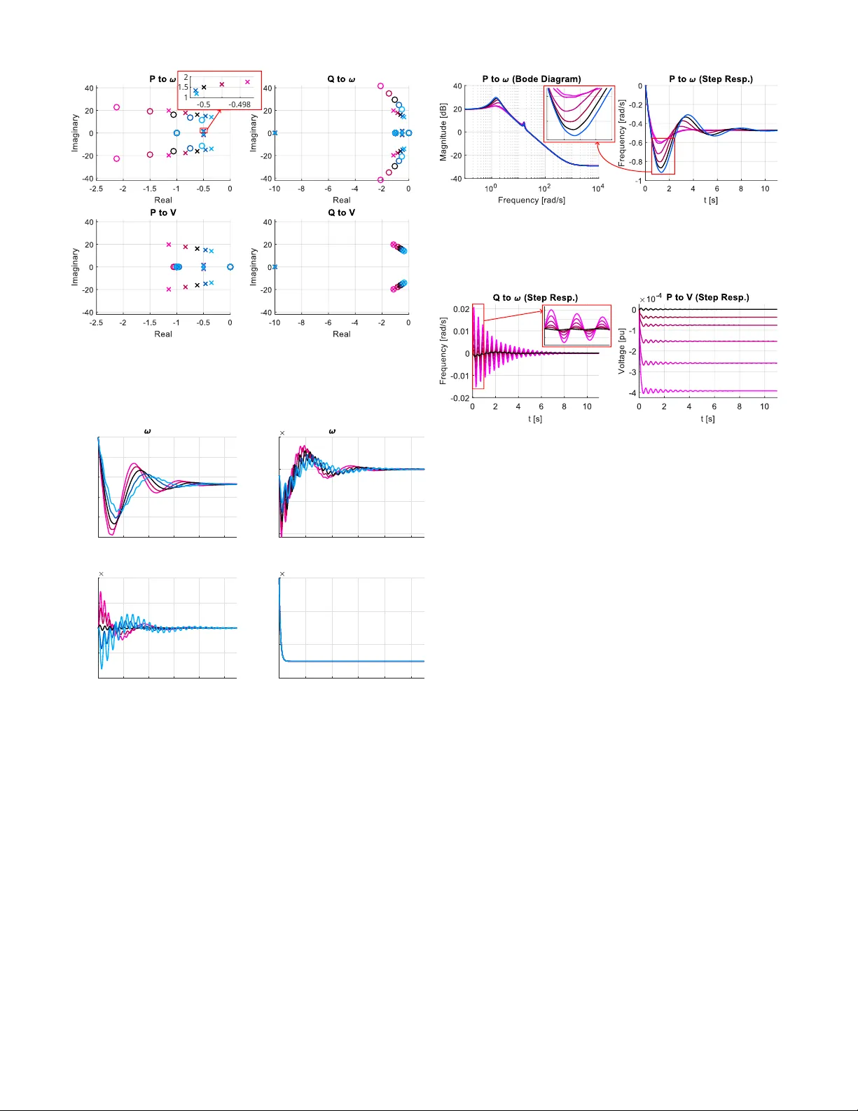
The role of VSG parameters in shaping small-signal SG dynamics Ferdinand Geuss University of Stuttgart Stuttgart, Germany ferdinand.geuss@isys.uni-stuttgart.de Orcun Karaca ABB Corporate Resear ch Baden-D ¨ attwil, Switzerland orcun.karaca@ch.abb .com Mario Schweizer ABB Corporate Resear ch Baden-D ¨ attwil, Switzerland mario.schweizer@ch.abb .com Ognjen Stanoje v ABB Corporate Resear ch Baden-D ¨ attwil, Switzerland ognjen.stanojev@ch.abb .com Abstract —W e derive a small-signal transfer function for a system comprising a virtual synchronous generator (VSG), a synchronous generator (SG), and a load, capturing v oltage and frequency dynamics. Using this model, we analyze the sensitivity of SG dynamics to VSG parameters, highlighting trade-offs in choosing virtual inertia and governor lag, the limited effect of damper -winding emulation, and several others. Index T erms —virtual synchronous generator , virtual inertia, grid-forming control I . I N T R O D U C T I O N As power electronic interf aces become more pre valent, particularly with the rene wable integration, the industry in- creasingly requires adv anced grid-forming (GFM) control. These controllers can form v oltage, emulate inertia, and realize droop behavior . For such controllers, small-signal methods are widely used especially in single grid-connected con- verter systems, e.g., with passi vity or Nyquist criteria [1]. In contrast, this paper studies the small-signal properties of an interconnected system comprising a con verter operated as a virtual synchronous generator (VSG) 1 , a synchronous generator (SG), and a load. Unlike the related studies in [2]– [5], the current control and the network dynamics are neglected to focus only on slower dynamics. Such simplified models can rev eal beha viors that more detailed models may obscure. This same motiv ation led to the foundational work in [6], which deliberately overlook ed network dynamics to deriv e a parallel VSG–SG model, unv eiling new facets of VSG parametriza- tion. Howe ver , that study omits voltage and reactiv e power dynamics, does not analyze zero locations or their impact, and primarily highlights the benefits of higher inertia/damping and reduced gov ernor delay . These limitations motiv ate our work, and we address each explicitly . Among more detailed models, [2] considers simulation studies for a nine-bus system, including the dc-link and current control dynamics, highlighting the interaction between fast GFM control and slow SG dynamics. A small-signal study of parallel VSGs in [3] determines their damping coefficients. In [4], a small-signal model of a VSG-SG interconnection with network dynamics is deri ved to study low-frequenc y oscillations using pole plots. They state that increasing the 1 Referring primarily to droop control, inertia, and damper winding emula- tion functionalities present in GFM. gov ernor lag and inductance could weaken the influence of the VSG. Related simplified models are found in [7]–[11]. For ex- ample, [7] analyzes instability with grid-follo wing (GFL) penetration; [8] sho ws damping v ersus penetration le vels; [9] deriv es a VSG small-signal model highlighting the coupling of QV and P ω dynamics; [10] studies a GFL conv erter connected to a VSG; and [11] examines inertia and damping effects in different time interv als during a frequency transient. The main contribution of this paper is the deriv ation of a small-signal transfer function mapping load power to inter- nal frequencies and voltages, which we use to analyze the interconnected system with respect to VSG parametrization, in particular, to study the sensiti vity of SG dynamics. Com- pared with [6], the transfer function also captures voltage and reactive po wer dynamics, and we giv e specific attention to the locations of its zeros. Section IV sho ws that these zero locations can significantly affect system behavior . In our analysis, we vary VSG parameters—inertia, damper winding constant, governor lag time constant, QV -droop gain and filter time constant, stator inductance, and XR-ratio—one at a time while keeping others at nominal values, to provide insights. These insights either confirm or extend prior findings. For example, we confirm the results of [4] (discussed abo ve), further distinguish oscillations on two distinct time scales, and examine the influence of zeros in both activ e and reactive power dynamics. Compared with [10], we also confirm the benefits of increased inertia, but we further highlight the advantages of inertia matching. Finally , we validate the trans- fer function and the main findings through simulation case studies. I I . P R E L I M I N A R I E S Parameters are denoted with upper-case, e.g., K . Bold cap- itals, e.g., K , refer to parameter matrices, and K ij describes the entry in the i th ro w and j th column of K . The identity is I . Functions in upper-case refer to transfer functions, e.g., G ( s ) , while transfer function matrices are bold, e.g., G ( s ) . Here, s is to be interpreted as the deri vati ve operator . Scalar v ariables are expressed by lower -case, such as v , and their vector versions are denoted bold, e.g., v . Phasors are marked by an arrow , e.g.,  v = v · e j φ = v  φ . Subscripts v , s , b are used to distinguish quantities belonging to the VSG, the SG, and Fig. 1. Diagram of the VSG model. the bus, respectively . Similarly , references are indicated by the subscript r . For example, the reference frequency is ω r . For bre vity , we often define quantities only for the VSG or only for the SG. Next, we describe the dynamics and the assumptions, and present the interconnected system. A. VSG Modeling The VSG dynamics follow [6], with the difference that we include v oltage dynamics (see Fig. 1). As in [6], the SG has the same structure as the VSG, with different parametrization. The VSG is modeled as a three-phase voltage source with magnitude v v and instantaneous phase angle φ v (i.e., with frequenc y ω v = sφ v ) in series with a virtual stator impedance Z v . In contrast to the pure inductances in [6], we hav e resistive-inducti ve impedances, i.e., Z v = R v + j ω r L v = R v + j X v . Small-signal changes in the reactance are similarly ignored. The VSG is connected to a bus with magnitude v b and instantaneous phase angle φ b (i.e., ω b = sφ b ), and the complex power at the line connecting to this bus is denoted by s v = [ p v q v ] ⊤ in vector-form, where p v and q v refer to active and reacti ve power , respecti vely . 1) F r equency Dynamics: The dynamics of ω v are gov erned by the swing equation, i.e., M v sω v = p v , r − K p , v ( ω v − ω r ) 1 + T p , v s − p v − D v ( ω v − ω b ) , (1) with angular momentum M v , assuming M v = J v ω r . J v = 2 H v ω 2 r S n refers to the moment of inertia, where H v and S n are the inertia time constant and the nominal power , respectively . The first term on the right-hand side of (1), including the power setpoint p v , r and the frequency droop with constant K p , v , describes the speed governor . T o model the typical delay of the prime mover , a low-pass filter with time constant T p , v is included. For a VSG, T p , v can be lower than that of a real SG. The third term approximates the ef fect of the damper windings. It is dependent on the dif ference between internal frequency and bus frequency through a damper winding constant D v . 2) V oltage Dynamics: The v oltage dynamics are gi ven by v v = v v , r + ( K q , v / (1 + T q , v s )) ( q v , r − q v ) . (2) The internal voltage magnitude v v is determined by QV -droop, i.e., linear around its setpoint v v , r based on the difference between q v and its setpoint q v , r via the droop constant K q , v . Similar to the speed gov ernor , the QV -droop is also subject to delays, modeled by a lo w-pass filter with time constant T q , v . Fig. 2. Diagram of the interconnected system model. 3) P ower Flow: The quasi-steady state output po wer sup- plied to the b us node with v oltage  v b is giv en by p v =Re {  v b  i ∗ v } = R v  v v v b cos( θ v ) − v 2 b  + X v v v v b sin( θ v ) R 2 v + X 2 v , (3) q v =Im {  v b  i ∗ v } = X v  v v v b cos( θ v ) − v 2 b  − R v v v v b sin( θ v ) R 2 v + X 2 v , (4) where θ v = φ v − φ b denotes the angle dif ference over the stator impedance, also satisfying sθ v = ω v − ω b . B. Setup of the Inter connected System The VSG, SG, and load are directly connected to a common bus (Fig. 2).The SG and VSG share the same dynamics with different parametrization, and the load power is s L = s v + s s . Line impedances between the VSG and SG are assumed negligible. Modeling them would require distinct bus nodes and additional equations, which we relegate to future work. I I I . S M A L L - S I G N A L D Y N A M I C S W e first deriv e a small-signal version of the VSG model, followed by its stand-alone operation and the complete system. For any x , let x = x 0 + ∆ x , where x 0 represents the steady-state value (i.e., operating point), while ∆ x denotes the perturbation variable. Small-signal representation of (1) is: M v s ∆ ω v = − ( K p , v / (1+ T p , v s ))∆ ω v − ∆ p v − D v (∆ ω v − ∆ ω b ) . (5) Similarly , the small-signal representation of (2) is ∆ v v = − ( K q , v / (1 + T q , v s )) ∆ q v . (6) Notice that (3) and (4) are nonlinear . T o this end, we linearize (3) and (4) with respect to θ v , v v , and v b . Separating operating points and perturbation v ariables, we get ∆ s v = [∆ p v ∆ q v ] ⊤ = K v [∆ θ v ∆ v v ∆ v b ] ⊤ , (7) with the power flo w matrix K v as in (8) (provided on top of the next page). Finally , we ha ve ∆ θ v = ∆ φ v − ∆ φ b , s ∆ θ v = ∆ ω v − ∆ ω b , (9) to describe the relati ve angle dif ference and its deriv ative. K v = " − R v v v , 0 v b , 0 sin( θ v , 0 )+ X v v v , 0 v b , 0 cos( θ v , 0 ) R 2 v + X 2 v R v v b , 0 cos( θ v , 0 )+ X v v b , 0 sin( θ v , 0 ) R 2 v + X 2 v R v ( v v , 0 cos( θ v , 0 ) − 2 v b , 0 )+ X v v v , 0 sin( θ v , 0 ) R 2 v + X 2 v − R v v v , 0 v b , 0 cos( θ v , 0 ) − X v v v , 0 v b , 0 sin( θ v , 0 ) R 2 v + X 2 v − R v v b , 0 sin( θ v , 0 )+ X v v b , 0 cos( θ v , 0 ) R 2 v + X 2 v − R v v v , 0 sin( θ v , 0 )+ X v ( v v , 0 cos( θ v , 0 ) − 2 v b , 0 ) R 2 v + X 2 v # (8) A. Stand-Alone VSG Dynamics W e obtain a small-signal transfer function for Figure 1 as [∆ ω v ∆ v v ] ⊤ = G v ( s )∆ s v . W e first need to eliminate ∆ v b from (7) and ∆ ω b from (5) to relate the internal VSG dynamics only to the perturbation variables of po wer: ∆ p v and ∆ q v . T o this end, the follo wing is obtained by solving each row of (7) for ∆ θ v and eliminating ∆ θ v : ∆ p v − K v , 12 ∆ v v − K v , 13 ∆ v b K v , 11 = ∆ q v − K v , 22 ∆ v v − K v , 23 ∆ v b K v , 21 . Solving for ∆ v b yields ∆ v b = [ A p , v A q , v A v , v ][∆ p v ∆ q v ∆ v v ] ⊤ , (10) A p , v = − K v , 21 K v , 11 K v , 23 − K v , 13 K v , 21 , A q , v = K v , 11 K v , 11 K v , 23 − K v , 13 K v , 21 , A v , v = K v , 12 K v , 21 − K v , 11 K v , 22 K v , 11 K v , 23 − K v , 13 K v , 21 . T o eliminate ∆ ω b from (5), bring in the following from (7): s ∆ p v = [ K v , 11 K v , 12 K v , 13 ] s [∆ θ v ∆ v v ∆ v b ] ⊤ . Inserting (9) and (10) into the equation above, we get s ∆ p v = K v , 11 (∆ ω v − ∆ ω b ) + K v , 12 s ∆ v v + K v , 13 ( A p , v s ∆ p v + A q , v s ∆ q v + A v , v s ∆ v v ) . By reorganizing the terms above, we obtain ∆ ω v − ∆ ω b = 1 − K v , 13 A p , v K v , 11 s ∆ p v − K v , 13 A q , v K v , 11 s ∆ q v − K v , 12 + K v , 13 A v , v K v , 11 s ∆ v v . (11) T owards our goal, we can no w substitute (11) into (5), yielding M v s ∆ ω v = −  1+ D v 1 − K v , 13 A p , v K v , 11 s  ∆ p v − K p , v 1+ T p , v s ∆ ω v + D v K v , 13 A q , v K v , 11 s ∆ q v + D v K v , 12 + K v , 13 A v , v K v , 11 s ∆ v v . Finally , in voking (6), we get the follo wing for ∆ ω v : ∆ ω v = − 1+ D v K v , 11 (1 − K v , 13 A p , v ) s M v s + K p , v 1+ T p , v s ∆ p v + D v K v , 11  K v , 13 A q , v − K q , v 1+ T q , v s ( K v , 12 + K v , 13 A v , v )  M v s + K p , v 1+ T p , v s s ∆ q v . The v oltage dynamics are governed by (6). Hence, the small-signal transfer function for stand-alone VSG operation is G v ( s )= " G v , 11 ( s ) G v , 12 ( s ) 0 − K q , v 1+ T q , v s # , G v , 11 ( s )= − 1+ D v K v , 11 (1 − K v , 13 A p , v ) s M v s + K p , v 1+ T p , v s , G v , 12 ( s )= D v K v , 11  K v , 13 A q , v − K q , v 1+ T q , v s ( K v , 12 + K v , 13 A v , v )  M v s + K p , v 1+ T p , v s s. Analogously , b ut with a dif ferent parametrization, G s ( s ) can be obtained for the SG, satisfying [∆ ω s ∆ v s ] ⊤ = G s ( s )∆ s s . This is omitted in the interest of space. B. Interconnected System Dynamics Next, we derive the small-signal transfer function for the complete interconnected system as depicted in Figure 2. These transfer functions are of the following form: ∆ y v = [∆ ω v ∆ v v ] ⊤ = H L → v ( s )∆ s L , ∆ y s = [∆ ω s ∆ v s ] ⊤ = H L → s ( s )∆ s L . Similar to the stand-alone operation, the deri vation steps for VSG and SG are analogous. Given the focus of our sensitivity analysis, we present H L → s ( s ) . Defining ∆ y b = [∆ ω b ∆ v b ] ⊤ , our approach relies on an intermediate step by deri ving ∆ s v = F b , v ( s )∆ y b , ∆ s s = F b , s ( s )∆ y b , to then isolate either of the VSG or SG dynamics via elimi- nation of certain terms by substitution. 1) Intermediate Step: Multiplying both sides of (7) by s , substituting (9), and separating terms dependent on ∆ ω v and ∆ v v from terms dependent on ∆ ω b and ∆ v b results in s ∆ s v = K v   ∆ ω v − ∆ ω b s ∆ v v s ∆ v b   = B v , v ( s )∆ y v + B b , v ( s )∆ y b , (12) B v , v ( s ) =  K v , 11 K v , 12 s K v , 21 K v , 22 s  , B b , v ( s ) =  − K v , 11 K v , 13 s − K v , 21 K v , 23 s  . For the SG, we have the following version of the abov e: s ∆ s s = K s   ∆ ω s − ∆ ω b s ∆ v s s ∆ v b   = B s , s ( s )∆ y s + B b , s ( s )∆ y b . (13) B s , s ( s ) and B b , s ( s ) are omitted in the interest of space. W e can no w obtain ∆ s v in terms of ∆ y b . Inserting ∆ y v = G v ( s )∆ s v into (12) and solving for ∆ s v yields ∆ s v = F b , v ( s )∆ y b , (14) where F b , v ( s ) = ( s I − B v , v ( s ) G v ( s )) − 1 B b , v ( s ) . A similar expression can also be obtained for the SG as follo ws: ∆ s s = F b , s ( s )∆ y b , (15) where F b , s ( s ) = ( s I − B s , s ( s ) G s ( s )) − 1 B b , s ( s ) . 2) Complete T ransfer Function for the SG: W e deri ve the small-signal transfer function H L → s ( s ) from ∆ s L to ∆ y s . Inserting in verse of (15) into (13) results in s ∆ s s = B s , s ( s )∆ y s + B b , s ( s ) F − 1 b , s ( s )∆ s s , and solving for ∆ s s giv es ∆ s s =  s I − B b , s ( s ) F − 1 b,s ( s )  − 1 B s , s ( s )∆ y s . (16) Notice that if we can relate ∆ s s to ∆ s L , the deri vation is complete. T o this end, insert (14) and (15) into ∆ s L = ∆ s v + ∆ s s , and then substitute in verse (15) to eliminate ∆ y b : ∆ s L = ( F b , v ( s ) + F b , s ( s )) F − 1 b , s ( s )∆ s s . (17) Combine (16) and (17) to obtain ∆ y s = H L → s ( s )∆ s L : H L → s ( s ) =  ( F b , v ( s ) + F b , s ( s )) F − 1 b , s ( s ) ×  s I − B b , s ( s ) F − 1 b , s ( s )  − 1 B s , s ( s )  − 1 . (18) Remark. The same method also applies when deriving the transfer function H L → v ( s ) for the VSG. The final result is H L → v ( s ) =  ( F b , v ( s ) + F b , s ( s )) F − 1 b , v ( s ) ×  s I − B b , v ( s ) F − 1 b , v ( s )  − 1 B v , v ( s )  − 1 . I V . S E N S I T I V I T Y A N A L Y S I S This section analyzes the sensitivity of SG dynamics in the interconnected system to variations of VSG parameters All quantities are per-unit except time, frequency , and angles. Bases are: nominal power of SG/VSG S n = 1 MV A, base voltage V n = 6 . 6 kV (phase-phase RMS), and nominal frequency ω n = 2 π 60 rad/s, ω r = ω n . Parameters largely follow [6], except we adopt a large SG delay T p , s to reflect typically slow SG governors and prime movers [4], [7]. This base case is listed in T able I. The VSG’ s default damper- winding constant is larger than the SG’ s, and all remaining parameters match. As in [6], the SG and VSG include no stator resistance in the base case. Later , we vary the VSG’ s XR-ratio. Power flow matrices K v and K s are dependent on the operating point v v , 0 , v s , 0 , v b , 0 , θ v , 0 , and θ s , 0 , obtained by solving the po wer flo w equations (3) and (4). W e set p v , 0 = p s , 0 = 0 . 5 pu, q v , 0 = q s , 0 = 0 . 5 pu, and v b , 0 = 1 pu. T ABLE I D E F AU LT PAR A M E TE R S F O R T HE S E N SI T I V IT Y A NA LYS E S . VSG SG Inertia constant H · 4 . 0 s 4 . 0 s Damper winding constant D · 17 pu 3 pu Frequency droop K p , · 20 pu 20 pu Governor lag T p , · 1 . 0 s 1 . 0 s QV droop K q , · 0 . 1 pu 0 . 1 pu QV droop lag T q , · 0 . 1 s 0 . 1 s Stator resistance R · 0 . 0 pu 0 . 0 pu Stator reactance X · 0 . 2 pu 0 . 2 pu T ABLE II O P ER ATI N G P O I N T F O R T H E S E N SI T I VI T Y A NA L Y S ES . v v , 0 1 . 1045 pu θ v , 0 0 . 0907 rad v s , 0 1 . 1045 pu θ s , 0 0 . 0907 rad v b , 0 1 . 0000 pu The resulting steady-state voltages and angles are in T able II. Sensitivity results hav e also been checked at other set points with similar observ ations. All transfer functions are stable with large mar gins, so further details are omitted. A. Sensitivity W ith Respect to H v The inertia constant is varied within [2 , 8] s. Fig. 3 shows poles and zeros for all four partial transfer functions of H L → s ( s ) in (18). These four transfer functions are always referred to as P → ω , Q → ω , P → V , and Q → V in the following, i.e., H L → s ( s ) =  P → ω Q → ω P → V Q → V  . The base case in T able I is plotted in black. Shades of red and blue denote smaller and larger inertia, respectiv ely . Step responses are shown in Fig. 4. Step responses use ∆ p L = ∆ q L = 0 . 05 pu. For visualizations, pole–zero pairs are canceled in plots using MA TLAB’ s minreal with tolerance 0 . 001 . 1) Observations on the Base Case: In the base case plotted in black, P → ω and Q → ω show a slow resonant pole pair (here referred to as the primary pole pair), resulting in a slow oscillatory behavior in the step response. All four transfer functions also exhibit a fast resonant pole pair (here called the secondary pole pair), which is partially canceled up to varying degree by accompanying zeros, except in P → V . Because of incomplete pole-zero cancellation, these faster oscillations are superimposed on the step response of P → ω and Q → ω . The cancellation is close to being perfect in Q → V . 2) Observations on Inertia: As Figs. 3 and 4 show , increas- ing H v leads to a better damping ratio and a decline of the nat- ural frequenc y of the primary pole pair for P → ω and Q → ω , reconfirming related observations in [6], [7], [10], [12]. For H v  = H s , the primary pole pair is also present in P → V . By contrast, the secondary poles shift to lo wer natural frequency and reduced damping for lar ger H v , consistent -0.5 -0.498 1 1.5 2 Fig. 3. Pole-zero plots for inertia constants in the range H v ∈ [2 , 8] s. ( Black : base case H v = 4 s, red : H v smaller than default, blue : H v larger than default. Darker shades refer to parameter values closer to the base case. Crosses refer to poles, circles indicate zeros.) 0 2 4 6 8 10 t [s] -1 -0.8 -0.6 -0.4 -0.2 0 Frequency [rad/s] P to (Step Resp.) 0 2 4 6 8 10 t [s] -2 -1 0 1 Frequency [rad/s] 10 -3 Q to (Step Resp.) 0 2 4 6 8 10 t [s] -1 -0.5 0 0.5 1 Voltage [pu] 10 -4 P to V (Step Resp.) 0 2 4 6 8 10 t [s] -3 -2 -1 0 Voltage [pu] 10 -3 Q to V (Step Resp.) Fig. 4. Step response plots for inertia constants in the range H v ∈ [2 , 8] s. ( Black : base case H v = 4 s, red : H v smaller than default, blue : H v larger than default. Darker shades refer to parameter values closer to the base case.) with transient damping observations for inertialess droop con- trollers [13]. Zero–pole cancellation is best (in terms of natural frequency) when H v = H s . Accordingly , the step response of P → ω shows the smallest superimposed secondary oscil- lations at H v = H s . Thus, changes in pole–zero cancellation with H v can affect dynamics as much as pole locations. Q → ω e xhibits primary oscillations that decrease with larger H v , similar to P → ω . Secondary oscillations are slo wer to decay as H v increases. P → V contains large real zeros for H v  = H s , which are omitted in Fig. 3 for clarity , and which grow in magnitude for increasing mismatch, yielding stronger primary and secondary oscillations. In Q → V , secondary resonant poles are ef fectiv ely can- Fig. 5. Bode magnitude plots and step responses of P → ω for T p , v ∈ [0 . 03 , 1 . 3] s. ( Black : base case T p , v = 1 s, red : T p , v smaller than default, blue : T p , v larger than default. Darker shades refer to parameter values closer to the base case.) Fig. 6. Step responses plots of Q → ω and P → V for various X v /R v - ratios. ( Black : base case X v /R v = ∞ , r ed : X v /R v ∈ [2 , 20] . Darker shades refer to larger ratios.) celed and the real pole is insensitiv e to H v . Q → ω and P → V are at least an order of magnitude smaller than P → ω and Q → V due to the base case not including stator resistances. B. Sensitivity W ith Respect to T p , v Bode diagrams and step responses of P → ω for VSG gov ernor-lag variations T p , v ∈ [0 . 03 , 1 . 3] s (nominal T p , v = 1 s) are shown in Fig. 5. Increasing T p , v strengthens primary oscillations, whereas small T p , v effecti vely damps them, consistent with [4, §3.C], [6]. Con versely , secondary oscillations decrease with larger T p , v , revealing a trade-off. Q → V is largely unaffected by T p , v , and is omitted. C. Sensitivity W ith Respect to the XR-ratio Fig. 6 shows step responses of Q → ω and P → V for X v /R v ∈ { 2 , 3 , 5 , 10 , 20 , ∞} ; X v is fixed at its default and R v is varied. P → ω is unaffected over this range. Although not plotted, Q → V shows stronger secondary oscillations for smaller X v /R v . In general, Q → ω and P → V oscillations grow as X v /R v decreases. For Q → ω , secondary oscil- lations become dominant at small X v /R v , making primary oscillations negligible. A similar observation has also been provided in [4, §3.C] showing that decreasing the XR-ratio of VSG weakens the damping of lo w frequency oscillations. For P → V , the XR-ratio also shifts the steady-state value and a smaller ratio yields slightly larger secondary oscillations. D. Additional Results In this section, we list studies relegated to the appendix. Some of the main findings are later highlighted in Section V. Appendix A provides Bode magnitude plots for sensitivity with respect to H v and an alternativ e base case with matched damper winding constants for the SG and VSG. It also includes sensiti vities to D v , K q , v , T q , v , and X v . Finally , Appendix B validates the analytical model of Section III and the major observations via simulation case studies. V . C O N C L U S I O N W e deriv ed a small-signal model to analyze how the VSG parameters influence the SG dynamics. Our main findings from the sensitivity analysis are: (i) F or inertia, there is a trade-off between suppressing primary oscillations by choosing larger values and increasing secondary oscillations when deviating from H v = H s . (ii) A larger damper winding constant reduces secondary oscillations but is not effecti ve in damping primary ones. (iii) Matched impedance for VSG and SG yields smaller secondary oscillations. (iv) Smaller gov ernor lag strongly reduces primary oscillations, ev en though this might induce slightly stronger secondary oscillations. (v) No negati ve ef fects from mismatch in QV -droop are observed. Stator impedance and QV -droop control together how the voltage reacts to a change in reactiv e power . (vi) The magnitude of oscillations grow with decreasing XR-ratio of VSG. R E F E R E N C E S [1] L. Harnefors, X. W ang, A. G. Y epes, and F . Blaabjerg, “Passi vity- based stability assessment of grid-connected vscs—an overvie w , ” IEEE JESTPE , vol. 4, no. 1, pp. 116–125, 2015. [2] A. T ayyebi, D. Groß, A. Anta, F . Kupzog, and F . D ¨ orfler , “Frequency stability of synchronous machines and grid-forming power converters, ” IEEE JESTPE , vol. 8, no. 2, pp. 1004–1018, 2020. [3] P . Sun, J. Y ao, Y . Zhao, X. F ang, and J. Cao, “Stability assessment and damping optimization control of multiple grid-connected virtual synchronous generators, ” IEEE T rans. on Ener gy Conver s. , vol. 36, no. 4, pp. 3555–3567, 2021. [4] H. Liu, D. Sun, P . Song, X. Cheng, F . Zhao, and Y . T ian, “Influence of virtual synchronous generators on low frequency oscillations, ” CSEE J. of P ower and Energy Sys. , vol. 8, no. 4, pp. 1029–1038, 2022. [5] N. Pogaku, M. Prodanovic, and T . C. Green, “Modeling, analysis and testing of autonomous operation of an inverter -based microgrid, ” IEEE T rans. on P ower Elec. , vol. 22, no. 2, pp. 613–625, 2007. [6] J. Liu, Y . Miura, and T . Ise, “Comparison of dynamic characteristics between virtual synchronous generator and droop control in in verter - based distributed generators, ” IEEE T rans. on P ower Elec. , vol. 31, no. 5, pp. 3600–3611, 2016. [7] Y . Lin, B. Johnson, V . Gev orgian, V . Purba, and S. Dhople, “Stability assessment of a system comprising a single machine and inv erter with scalable ratings, ” in N APS , 2017, pp. 1–6. [8] R. H. Lasseter, Z. Chen, and D. Pattabiraman, “Grid-forming inverters: A critical asset for the power grid, ” IEEE JESTPE , vol. 8, no. 2, pp. 925–935, 2019. [9] H. W u, X. Ruan, D. Y ang, X. Chen, W . Zhao, Z. Lv , and Q.-C. Zhong, “Small-signal modeling and parameters design for virtual synchronous generators, ” IEEE T rans. on Ind. Elec. , vol. 63, no. 7, pp. 4292–4303, 2016. [10] S. D’Arco and J. A. Suul, “Small-signal analysis of an isolated power system controlled by a virtual synchronous machine, ” in IEEE PEMC , 2016, pp. 462–469. [11] D. Li, Q. Zhu, S. Lin, and X. Bian, “ A self-adaptiv e inertia and damping combination control of vsg to support frequency stability , ” IEEE Tr ans. on Energy Conver s. , vol. 32, no. 1, pp. 397–398, 2016. [12] A. E. Leon and J. M. Mauricio, “V irtual synchronous generator design to improv e frequency support of converter -interfaced systems, ” IEEE T rans. on Energy Convers. , 2024. [13] X. He, S. Pan, and H. Geng, “T ransient stability of hybrid po wer systems dominated by different types of grid-forming devices, ” IEEE T rans. on Ener gy Conver s. , vol. 37, no. 2, pp. 868–879, 2021. 10 0 10 2 10 4 Frequency [rad/s] -40 -20 0 20 40 Magnitude [dB] P to (Bode Diagram) 10 0 10 2 10 4 Frequency [rad/s] -80 -60 -40 -20 Magnitude [dB] Q to (Bode Diagram) 10 0 10 2 10 4 Frequency [rad/s] -200 -150 -100 -50 0 Magnitude [dB] P to V (Bode Diagram) 10 0 10 2 10 4 Frequency [rad/s] -100 -80 -60 -40 -20 Magnitude [dB] Q to V (Bode Diagram) Fig. 7. Bode magnitude plots for inertia constants in the range H v ∈ [2 , 8] s. ( Black : base case H v = 4 s, red : H v smaller than default, blue : H v larger than default. Darker shades refer to parameter values closer to the base case.) A P P E N D I X A A D D I T I O NA L S E N S I T I V I T Y A NA LY S E S A. Sensitivity W ith Respect to H v Bode magnitude plots are provided in Fig. 7. B. Base Case W ith Matching Damper W inding Constants When all the parameters including the damper winding constant are matched between the VSG and the SG, the secondary poles and zeros completely vanish from all partial transfer functions and P → V fully reduces to 0 . The resulting pole-zero plots are provided in Fig. 8. The primary poles remain unaffected. Hence, the matched parameters case yields a less complex dynamics structure free from any secondary dynamics. C. Sensitivity W ith Respect to D v Fig. 4 shows that larger inertia yields stronger secondary oscillations. Hence, lar ger inertia H v = 2 H default v is chosen such that the effect of v ariations in D v is more pronounced. Q → V is insensitiv e to changes in D v . Thus, Fig. 9 provides only the Bode plots and step responses of P → ω for damper winding constants in [0 . 3 , 34] pu, where D v = 17 pu by default. D v has no ef fect on the primary resonant poles, and the primary oscillations remain intact. The secondary oscillations decrease for larger damper winding constants. While the degree of pole-zero cancellation does not change with D v , the pole damping increases with growing D v . D. Sensitivity W ith Respect to K q , v W e again use H v from T able I. V arying K q , v within [0 . 05 , 0 . 2] pu (default: K q , v = 0 . 1 pu) has virtually no ef fect on the dynamics of P → ω , Thus, Fig. 10 only shows Q → V . The dynamic behaviour of Q → V remains mostly unaffected by the changes in K q , v , and only the steady-state value dif fers. -2.5 -2 -1.5 -1 -0.5 0 Real -40 -20 0 20 40 Imaginary P to -10 -8 -6 -4 -2 0 Real -40 -20 0 20 40 Imaginary Q to -2.5 -2 -1.5 -1 -0.5 0 Real -40 -20 0 20 40 Imaginary P to V -10 -8 -6 -4 -2 0 Real -40 -20 0 20 40 Imaginary Q to V Fig. 8. Pole-zero plots for a modified base case when the VSG parameters perfectly match the SG parameters. ( Black : modified base case. Crosses refer to poles, circles indicate zeros.) Fig. 9. Bode magnitude plots and step responses of P → ω for D v ∈ [0 . 3 , 34] p.u with H v = 2 H default v for all. ( Black : base case D v = 17 pu, red : D v smaller than default, blue : D v larger than default. Darker shades refer to parameter values closer to the base case.) Thus, the choice of K q , v should depend on the desired droop lev el. E. Sensitivity W ith Respect to T q , v Fig. 11 sho ws the Bode plots and step responses of Q → V for changing QV -droop time constants in the range [0 . 05 , 0 . 2] s, where T q , v = 0 . 1 s by default. W e observe that T q , v has no effect on P → ω . While not easily observed in the figure, Q → V contains a second real pole for T q , v  = T q , s , and for smaller lag T q , v , a slightly faster con vergence of the step response is observ ed. F . Sensitivity W ith Respect to X v X v is varied within [0 . 1 , 0 . 4] pu, with the nominal value being X v = 0 . 2 pu. The choice of X v also af fects the oper- ating point of the system, and we recompute it accordingly . The Bode plots of P → ω and Q → V are shown in Fig. 12. While X v has no effect on the primary poles of P → ω , the location of its secondary poles and zeros changes, and the best pole-zero cancellation appears to be achie ved for X v = X s . Hence, matching impedances has significant importance. In the mismatched case, an additional fast real pole appears in 10 0 10 2 10 4 Frequency [rad/s] -100 -80 -60 -40 -20 Magnitude [dB] Q to V (Bode Diagram) 0 0.2 0.4 0.6 0.8 1 t [s] -3 -2 -1 0 Voltage [pu] 10 -3 Q to V (Step Resp.) Fig. 10. Bode magnitude plots and step responses of Q → V for K q , v ∈ [0 . 05 , 0 . 2] pu ( Black : base case K q , v = 0 . 1 pu, r ed : K q , v smaller than default, blue : K q , v larger than default. Darker shades refer to parameter values closer to the base case.) 10 0 10 2 10 4 Frequency [rad/s] -100 -80 -60 -40 -20 Magnitude [dB] Q to V (Bode Diagram) 0 0.2 0.4 0.6 0.8 1 t [s] -2.5 -2 -1.5 -1 -0.5 0 Voltage [pu] 10 -3 Q to V (Step Resp.) Fig. 11. Bode magnitude plots and step responses of Q → V for T q , v ∈ [0 . 05 , 0 . 2] s. ( Black : base case T q , v = 0 . 1 s, red : T q , v smaller than default, blue : T q , v larger than default. Darker shades refer to parameter values closer to the base case.) Q → V , and it becomes slower as X v increases. But ev en then, the main difference lies in this transfer function’ s steady- state v alue. As expected, the change in voltage magnitude in response to the same step is larger for bigger X v . G. T uning Guidelines Here, we provide a set of additional numerical tuning guide- lines for the VSG in the specific system under consideration based on the analytical models and previous observations: (i) Letting H v ∈ [4 , 5] s ensures a good trade-of f between the benefits of matching inertia and having slightly larger inertia. (ii) Setting D v ≥ 17 pu eliminates the secondary oscillations in P → ω . (iii) Matching X v = X s , and keeping the XR-ratio of the VSG high are both indispensable. (iv) Having a gov ernor lag T p , v ∈ [0 . 06 , 0 . 12] s is desirable, as much lower values could create further oscillations. (v) Finally , QV -droop lag can be lower for the VSG, e.g, T q , v = 0 . 05 s, to ha ve slightly faster con ver gence. A P P E N D I X B S I M U L A T I O N C A S E S T U D I E S This section verifies the analytical model deriv ed in Section III and some of the major observations with simulation case studies. W e first explain the simulation setup and implementation to then provide step responses for activ e and reactive po wer steps. W e vary H v , X v , XR-ratio, and the load impedance. 10 0 10 2 10 4 Frequency [rad/s] -40 -20 0 20 40 Magnitude [dB] P to (Bode Diagram) 10 0 10 2 10 4 Frequency [rad/s] -100 -80 -60 -40 -20 Magnitude [dB] Q to V (Bode Diagram) Fig. 12. Bode magnitude plots of P → ω and Q → V for X v ∈ [0 . 1 , 0 . 4] pu ( Black : base case X v = 0 . 2 pu, red : X v smaller than default, blue : X v larger than default. Darker shades refer to parameter values closer to the base case.) Fig. 13. Diagram of the simulation model. The system is implemented in MA TLAB/Simulink. Fig. 13 shows its diagram. The grid model includes resistive-inducti ve line impedances. Idealized controlled v oltage sources with input signals  v v and  v s provide the internal voltages, assum- ing av erage conv erter models. The load is modeled by the two impedances Z L , 0 and Z L , step , the val ues of which are determined to create the operating point and the power step. The step is performed by closing the switch sw step . Unless later mentioned otherwise, we use the parameters in T able I and the line impedances Z line = 0 . 0054 + 0 . 0076 j pu, matching [6]. The system is initialized to s v , r = s s , r = [0 . 5 0 . 5] ⊤ pu and the operating point described in T able II. The impedance Z L , step is set to ensure a load step of ∆ s L = [0 . 02 0 . 02] ⊤ pu. Power flow matrices K v and K s depend on the voltage and angle operating points, and due to the line impedances, the real operating points slightly deviate from the precomputed solution of (3) and (4). Hence, the analytical step responses are obtained using the actual operating points obtained from the simulations. Since p L and q L are perturbed simultaneously , these simulation studies do not identify P → ω and Q → ω separately . Hence, we focus on the signals ∆ ω s and ∆ v s . A. V erification of the Small-Signal Model Fig. 14 compares the step response computed from the small-signal model to the one obtained from the simulations. The parameters are as described abov e, and Z L , 0 = 0 . 5 + 0 . 5 j pu and Z L , step = 25 + 25 j pu accordingly . As Fig. 14 shows, despite a minor mismatch during the transient, the simulation plots closely follo w the predictions. 0 5 10 t [s] -0.3 -0.2 -0.1 0 s [rad/s] Frequency simulated analytical 0 5 10 t [s] -8 -6 -4 -2 0 v s [pu] 10 -4 Voltage Fig. 14. Comparison of simulated and analytical step responses (base case). Fig. 15. Comparison of step responses for H v = 2 H default v . B. Case Studies for Differ ent P arameter Realisations W e no w vary the parameters. First, Fig. 15 sho ws the case where H v = 2 H default v . Second, the step responses for X v = 1 . 4 X default v are presented in Fig. 16. Third, Fig. 17 includes a nonzero stator resistance for the VSG: X v /R v = 3 . Finally , we sho wcase the use of different load impedances in Fig. 18: s v ,r = s s ,r = [0 . 5 0 . 25] ⊤ pu is chosen, such that Z L , 0 = 0 . 8 + 0 . 4 j pu. Furthermore, ∆ s L = [0 . 04 0 . 04] ⊤ pu yields Z L , step = 12 . 5 + 12 . 5 j pu. Setpoints, system initialisation, and power flo w matrices are adjusted accordingly . In all cases, the simulations support the analytical results. Fig. 15 shows smaller primary oscillations and stronger sec- ondary oscillations in the frequency step response than in Fig. 14, matching the findings from Section IV -A. Also, stronger secondary oscillations that can be attrib uted to P → V can be observed in the combined voltage step response. Similarly , the slightly stronger oscillations in the frequency step response of Fig. 16 and the larger voltage drop in steady-state due X v > X s support the analytical results from Section A-F. As discussed in Section IV -C, due to a lo w XR- ratio, we can observe stronger secondary oscillations in both, the frequency and the voltage step response of Fig. 17 than in the base case. In addition to that, Fig. 18 illustrates that simulations and analytical results also match for different loads and power settings. W e observe larger perturbations in frequency and voltage due to the bigger load step size. Fig. 16. Comparison of step responses for X v = 1 . 4 X default v . 0 5 10 t [s] -0.3 -0.2 -0.1 0 s [rad/s] Frequency simulated analytical 0 2 4 6 8 10 t [s] -8 -6 -4 -2 0 v s [pu] 10 -4 Voltage Fig. 17. Comparison of step responses for R v  = 0 pu such that X v /R v = 3 . 0 5 10 t [s] -0.6 -0.4 -0.2 0 s [rad/s] Frequency simulated analytical 0 5 10 t [s] -20 -15 -10 -5 0 v s [pu] 10 -4 Voltage Fig. 18. Comparison of step responses for changed power lev els and loads: s v ,r = s s ,r = [0 . 5 0 . 25] ⊤ pu and ∆ s L = [0 . 04 0 . 04] ⊤ pu, yielding Z L , 0 = 0 . 8 + 0 . 4 j pu and Z L , step = 12 . 5 + 12 . 5 j pu