Confidence Distributions for FIC scores

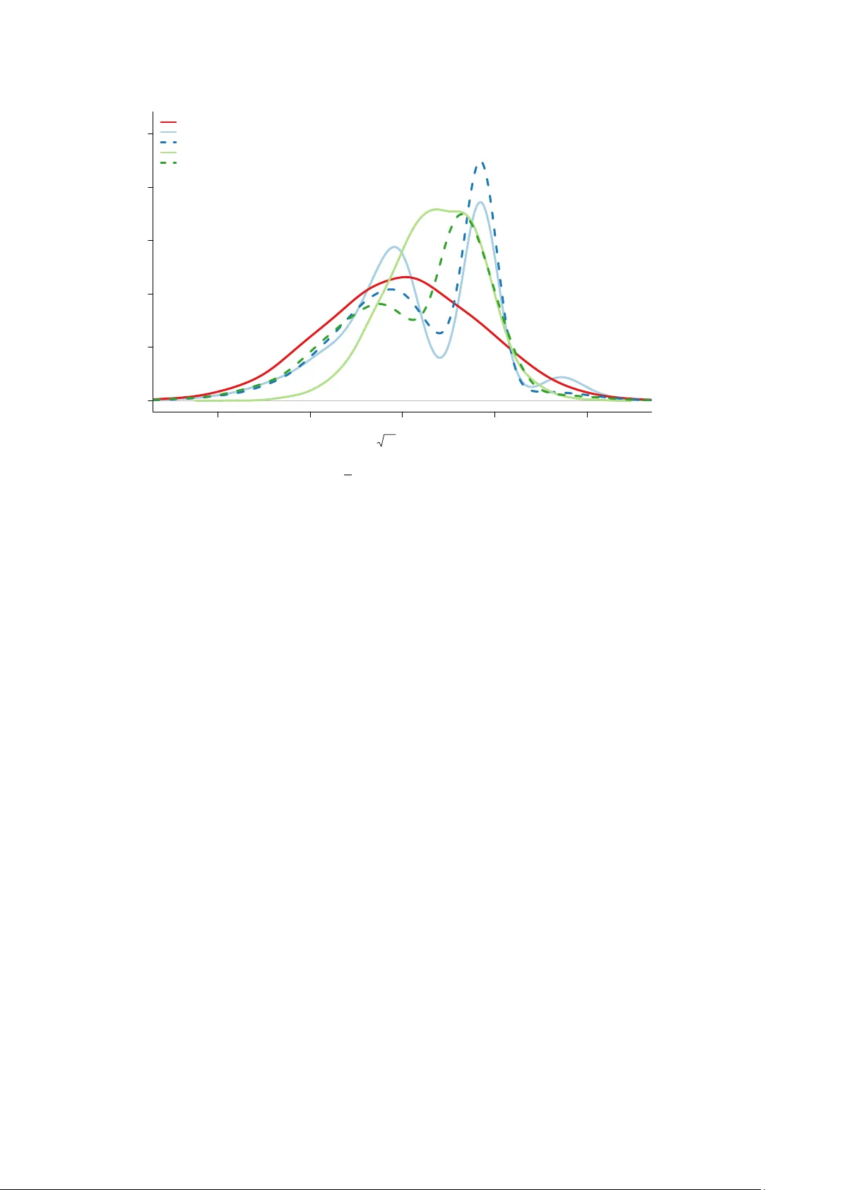
Confidence Distributions for FIC scores C ´ eline Cunen and Nils Lid Hjort Dep ar tment of Ma thema tics, University of Oslo December 2019 Abstract. When using the F o cused Information Criterion (FIC) for assessing and ranking candidate mo dels with respect to ho w well they do for a giv en estimation task, i t is customary to pro duce a so-called FIC plot. This plot has the differen t point estimates along the y-axis and the root-FIC scores on the x-axis, these b eing the estimated ro ot- mean-square scores. In this pap er we address the estimation uncertaint y inv olved in eac h of the p oints of such a FIC plot. This needs careful assessment of each of the estimators from the candidate mo dels, taking also mo delling bias into accoun t, along with the relativ e precision of the associated estimated mean squared error quantities. W e use confidence distributions for these endeav ours. This leads to fruitful CD-FIC plots, helping the statistician to judge to what extent the seemingly b est models really are better than other mo dels, etc. These efforts also lead to t wo further developmen ts. The first is a new tool for mo del selection, whic h we call the quantile-FIC, whic h helps ov ercome certain difficulties asso ciated with the usual FIC pro cedures, related to somewhat arbitrary sc hemes for handling estimated squared biases. A particular case is the median-FIC. The second dev elopment is to form model a veraged estimators with fruitful weigh ts determined b y the relative sizes of the median- and quantile-FIC scores. Key wor ds: FIC plots, fo cused information criteria, median-FIC and quantile-FIC, mo del av eraging, risk functions 1 Intr oduction and summar y Mrs. Jones is pregnan t. She’s white, 25 y ears old, a smok er, and of median weigh t 60 kg b efore pregnancy . What’s the c hance that her baby-to-come will b e small, with birth weigh t less than 2.50 kg (whic h would mean a case of neonatal medical worry)? Figure 1 gives a FIC plot , using the F ocused Information Criterion to displa y and rank in this case 2 3 = 8 estimates of this probability , computed via eight logistic regression mo dels, inside the class p = P { y = 1 | x 1 , x 2 , z 1 , z 2 , z 3 } = exp( β 0 + β 1 x 1 + β 2 x 2 + γ 1 z 1 + γ 2 z 2 + γ 3 z 3 ) 1 + exp( β 0 + β 1 x 1 + β 2 x 2 + γ 1 z 1 + γ 2 z 2 + γ 3 z 3 ) , where x 1 is age, x 2 is w eight before pregnancy , z 1 is an indicator for being a smok er, whereas z 2 and z 3 are indicators for b elonging to certain ethnic groups. The dataset in question comprises 189 mothers and babies, with these five cov ariates ha ving b een recorded (along with yet others; see Claeskens & Hjort (2008, Ch. 2) for further discussion). The eight mo dels corresp ond to pushing the ‘open’ cov ariates z 1 , z 2 , z 3 in and out of the logistic regression structure, while x 1 , x 2 are ‘protected’ cov ariates. The plot shows the p oint estimates b p for the 8 differen t submo dels on the v ertical axis and r o ot-FIC sc or es on the horizon tal axis. These are estimated risks, i.e. estimates of ro ot-mean-squared-errors. Crucially , the FIC scores do not merely assess the standard deviation of estimators, but also take the p otential biases on b oard, from using smaller models. Using the FIC ranking, as summarised both in the FIC table given in T able 1 and the FIC plot, therefore, we learn that submo dels 000 and 010 are the b est (where e.g. ‘010’ 1 indicates the mo del with z 2 on b oard but without z 1 and z 3 , etc.), associated with p oint estimates 0.282 and 0.259, whereas submo dels 100 and 011 are the ostensibly worst, with rather less precise p oin t estimates 0.368 and 0.226. Again, ‘best’ and ‘worst’ means as gauged b y precision of these 8 estimates of the same quantit y . Imp ortantly , the FIC machinery , as briefly explained here, with more details in later sections, can b e used for each new w oman, with different ‘b est mo dels’ for different strata of w omen, and it may be used for handling differen t and even quite complicated fo cus parameters. In particular, if Mrs. Jones had not b een a smok er, so that her z 1 = 1 w ould rather hav e b een a z 1 = 0, we run our programmes to pro duce a FIC table and a FIC plot for her, and learn that the submo del ranking is very differen t. Then 111 and 101 are the b est and 001 and 000 the worst; also, the b p estimates of her having a baby with small birth w eigh t are significantly smaller. 0.04 0.05 0.06 0.07 0.08 0.09 0.25 0.30 0.35 root−fic estimates of pr(small baby) f or Mrs Jones ● ● ● ● ● ● ● ● 000 100 010 001 110 101 011 111 Figure 1: FIC plot for the 2 3 = 8 models for estimating the probabilit y of having a small child, for Mrs. Jones (white, age 25, 60 kg, smok er). Here ‘101’ is the model where z 1 , z 3 in in and z 2 is out, etc. in-or-out b p stdev bias ro ot-FIC rank 1 0 0 0 0.282 0.039 0.000 0.039 1 2 1 0 0 0.368 0.055 0.061 0.082 7 3 0 1 0 0.259 0.042 0.000 0.042 2 4 0 0 1 0.267 0.048 0.000 0.048 3 5 1 1 0 0.342 0.057 0.037 0.068 5 6 1 0 1 0.351 0.056 0.045 0.072 6 7 0 1 1 0.226 0.054 0.063 0.083 8 8 1 1 1 0.303 0.060 0.000 0.060 4 T able 1: FIC table for Mrs. Jones: there are 2 3 = 8 submo dels, with absence-presence of z 1 , z 2 , z 3 indicated with 0 and 1 in column 2, follo w ed b y estimates b p , estimated standard deviation, estimated absolute bias, the ro ot-FIC score, which is also the Pythagorean combination of the stdev and the bias, and the mo del rank. The num bers are computed with formulae of Section 2. The FIC apparatus, initiated and dev elop ed in Claesk ens & Hjort (2003), Hjort & Claesk ens (2003a), Claeskens & Hjort (2008), has led to quite a rich literature; see com- men ts at the end of this section. FIC analyses ha ve differen t forms of output, qua FIC 2 tables (listing the b est candidate mo dels, along with estimates and ro ot-FIC scores, p erhaps supplemen ted with more information) and FIC plots. The general setup inv olves a selected quan tit y of particular in terest, say µ , called the fo cus parameter, and v arious candidate mo d- els, say S , leading to a collection of estimators b µ S . These carry ro ot-mean-squared-errors rmse S , and the ro ot-FIC scores are estimates of these ro ot-risks. The FIC plot displays (FIC 1 / 2 S , b µ S ) = ( d mse 1 / 2 S , b µ S ) for all candidate mo dels S, (1.1) as with Figure 1. The present pap er concerns going b eyond such FIC plots, inv estigating the precision of eac h display ed p oint. The p oin t estimates b µ S carry uncertaint y , as do the FIC scores. A more elab orate version of the FIC plot can therefore display the uncertaint y in volv ed, in b oth the v ertical and horizon tal directions. This aids the statistician in seeing whether go o d models are ‘clear winners’ or not, and whether the ostensibly b est estimates are gen uinely more accurate than others. In v arious concrete examples one also observ es that a few candidate mo dels app ear to be b etter than the rest. The metho dology of our paper makes it p ossible to assess to whic h extent the implied differences in FIC scores are significan t. Suc h insigh ts lead also to model av eraging strategies with w eigh ts giv en precisely to the b est mo dels for the giv en estimation purp ose. Our pap er pro ceeds as follows. In Section 2 we give the required mathematical back- ground, in v olving b oth the basic notation necessary and the k ey theorems ab out joint con- v ergence of classes of candidate model based estimators. These results also drive the devel- opmen t of confidence distributions for FIC scores, in Section 3. Flo wing from these results again is also a new v ariant for the FIC, which w e call the quan tile-FIC, where eac h ro ot mean squared error quantit y (rmse) is naturally estimated using an appropriate quan tile in the asso ciated confidence distribution. A special case is the median-FIC; details are given in Section 4. With such results on b oard, Section 5 then inv olves constructions of median-FIC driv en weigh ts for mo del a veraging op erations, where w e also give a precise large-sample description of the implied mo del av eraging estimators. In Section 6 we address p erformance and comparison issues, studying relev ant asp ects of ho w well different sc hemes b ehav e, from p ost-FIC to model a v eraging estimators. It is in particular seen that the p ost-median-FIC estimators ha ve certain adv antages o ver post-AIC sc hemes. T o displa y ho w our new CD-FIC based metho ds work in a s etup with considerably more candidate mo dels at play than with the 2 3 = 8 mo dels used for Mrs. Jones ab ov e, a multi-regression Poisson setup is work ed through in Section 7, inv olving abundance of bird sp ecies for 73 British and Irish islands. Then we sum up v arious salien t p oints in our discussion Section 8, and round off our pap er with a list of concluding remarks, some p ointing to further research, in Section 9. W e end our in tro duction section b y commen ting briefly on other relev ant w ork, first on the FIC front and then on model av eraging. Setting up FIC schemes inv olves finding go o d appro ximations to mse quan tities, and then constructing estimators for these. This pans out differen tly in differen t classes of models, and sometimes requires length y separate efforts, dep ending also on the type of interest parameter in fo cus. Claeskens & Hjort (2008) cov er a broad range of general i.i.d. and regression mo dels, using lo cal neighbourho o ds metho d- ology . Later extensions include Claesk ens et al. (2007) for time series mo dels, Gueuning & Claesk ens (2018) for highdimensional setups, Hjort & Claeskens (2006) and Hjort (2008) for semiparametric and nonparametric surviv al regression mo dels, Zhang & Liang (2011) for generalised additiv e mo dels, Zhang et al. (2012) for tobit mo dels, Ko, Hjort & Hobæk Haff 3 (2019) for copulae with tw o-stage estimation metho ds. Recent metho dological extensions and adv ances also include setups centred on a fixed wide mo del, with large-sample appro xi- mations not dep ending on the local asymptotics metho ds; see Jullum & Hjort (2017, 2019); Claesk ens, Cunen & Hjort (2019), along with ? for linear mixed mo dels. There is a growing list of application domains where FIC is finding practical and context-relev ant use, such as finance and economics (Brownlees & Gallo, 2008; Behl et al., 2012), peace researc h and p o- litical science (Cunen, Hjort & Nyg ˚ ard, 2020), so ciology (Zhang et al., 2012), marine science (Hermansen, Hjort & Kjesbu, 2016), etc. There is similarly a rapidly expanding literature on frequentist mo del av eraging pro cedures, as partly contrasted with Ba y esian versions; p ersp ectives for the latter are summarised in Ho eting et al. (1999). A broad framew ork for frequen tist a v eraging metho ds is dev elop ed in Hjort & Claesk ens (2003a); Claeskens & Hjort (2008), including precise large-sample descriptions for ho w such schemes actually p erform. W ang et al. (2009) give a broad review. In econometrics, Hansen (2007) studies mo del a v eraging for least squares pro cedures, and Magnus et al. (2009) compare frequen tist and Ba y esian av eraging metho ds. Optimal weigh ts are studied in Liang et al. (2011). The b o ok c hapter Chan et al. (2020) discusses optimal av eraging schemes for forecasting, where a cer- tain phenomenon is that simpler weigh ting metho ds sometimes p erform b etter than those in v olving extra lay ers of estimation to get closer to envisaged optimal weigh ts. 2 The basic setup and the FIC In this section we give the basic theoretical background and main results b ehind the FIC plots (1.1). It is conv enient to describe the i.i.d. setup first, and to describ e a canonical limit exp erimen t with the required basic quantities following from the relev ant assumptions. W e then briefly explain how the apparatus can b e extended also to general regression models, where it also turns out that the limit experiment is of exactly the same t yp e, only with somewhat more complex mechanisms lying b ehind the key ingredients. The key results describ ed in this section are behind the FIC plots and the FIC tables, such as Figure 1 and T able 1, and will also b e used in later sections to derive confidence distributions for risks. 2.1 The i.i.d. setup. Suppose we ha v e indep endent and identically distributed ob- serv ations, sa y y 1 , . . . , y n . Under study is a collection of candidate mo dels, ranging from a w ell-defined narro w mo del, parametrised as f narr ( y , θ ) with θ = ( θ 1 , . . . , θ p ) of dimension p , to a wide mo del, parametrised as f ( y , θ, γ ), with certain extra parameters γ = ( γ 1 , . . . , γ q ), signifying mo del extensions in different directions. The narrow mo del is assumed to be an inner p oint in the wider mo del, in the sense of f narr ( y , θ ) b eing equal to f ( y , θ, γ 0 ) for an in- ner parameter point γ 0 . There is consequently a total of 2 q candidate models, corresp onding to setting γ j parameters equal to or not equal to their n ull v alues γ 0 ,j , for j = 1 , . . . , q . In the regression framework studied b elow this w ould typically corresp ond to taking cov ariates in and out of the wide model. Assume now that a parameter µ is to b e estimated, with a clear statistical interpretation across candidate models. It ma y in particular be expressed as µ = µ ( θ , γ ) in the wide model. W e ma y then consider 2 q differen t candidate estimators, say b µ S based on the submo del S , with S a subset of { 1 , . . . , q } , corresp onding to the mo del having γ j as a parameter in the mo del when j ∈ S but with γ j set to their null v alues γ 0 ,j for j / ∈ S . Carrying out maximum lik eliho o d (ML) estimation in mo del S means maximising the log-likelihoo d 4 function ℓ n,S ( θ , γ S ) = P n i =1 log f ( y i , θ, γ S , γ 0 ,S c ), with γ S notation for the collection of γ j with j ∈ S , and similarly for γ 0 ,S c with the complemen t set. With ( b θ S , b γ S ) the ML estimators for submodel S , this leads to a collection of candidate estimators b µ S = µ ( b θ S , b γ S , γ 0 ,S c ) for S ∈ { 1 , . . . , q } . In particular w e ha v e b µ narr = µ ( b θ narr , γ 0 ) and b µ wide = µ ( b θ wide , b γ wide ), with ML estimation carried out in resp ectively the narrow p -dimensional and the wide ( p + q )-dimensional models. T o understand the b eha viour of all these candidate estimators, and to dev elop theory and metho ds for sorting them through, aiming at finding the b est, w e no w presen t a ‘mas- ter theorem’, from Hjort & Claeskens (2003a), Claesk ens & Hjort (2008, Chs. 5, 6). W e w ork inside a system of lo cal neigh b ourho o ds, where the real data-generating mechanism underlying our observ ations is f true ( y ) = f ( y , θ 0 , γ 0 + δ / √ n ) , (2.1) with some unknown δ = √ n ( γ − γ 0 ), seen as a lo cal model extension parameter; in particular, the true focus parameter b ecomes µ true = µ ( θ 0 , γ 0 + δ / √ n ). A few key quan tities now need prop er definition. W e start with the Fisher information matrix with inv erse, of the wide mo del, but computed at the n ull model: J = J 00 J 01 J 10 J 11 ! and J − 1 = J 00 J 01 J 10 J 11 ! . (2.2) Here blocks J 00 and J 00 are of size p × p , etc. The q × q matrix Q = J 11 = ( J 11 − J 10 J − 1 00 J 01 ) − 1 serv es a vital role. So do also ω = J 10 J − 1 00 ∂ µ ∂ θ − ∂ µ ∂ γ and τ 2 0 = ( ∂ µ ∂ θ ) t J − 1 00 ∂ µ ∂ θ , (2.3) with partial deriv atives ev aluated at the null mo del, and with these quantities v arying from fo cus parameter to fo cus parameter. Finally w e need to introduce the q × q matrices G S = π t S Q S π S Q − 1 , with Q S = ( π S Q − 1 π t S ) − 1 . W e ha v e G narr = 0 and G wide = I , the q × q identit y matrix, and note that T r( G S ) = | S | , the n um be r of elements in S . The master theorems driving muc h of the FIC and related theory are now as follo ws. First, D n = √ n ( b γ wide − γ 0 ) → d D ∼ N q ( δ, Q ) , (2.4) and, secondly , √ n ( b µ S − µ true ) → d Λ S = Λ 0 + ω t ( δ − G S D ) for eac h S ∈ { 1 , . . . , q } . (2.5) Here Λ 0 ∼ N(0 , τ 2 0 ), for the τ 0 giv en ab ov e, and Λ 0 and D are indep endent. This implies that the limit in (2.5) is normal, and w e can read off its bias ω t ( I − G S ) δ and v ariance τ 2 0 + ω t G S QG t S ω . The risk or mean squared error for this limit distribution is hence mse S = E Λ 2 S = τ 2 0 + ω t G S QG t S ω + { ω t ( I − G S ) δ } 2 = v ar S + bsq S , (2.6) 5 sa y , in the usual fashion a sum of a v ariance part v ar S and a squared bias part bsq S . With a slim S , there are many zeros in G S , leading to small v ariance but p otentially a bigger bias; with a fatter S , G S b ecomes closer to the identit y matrix I , yielding bigger v ariance but a smaller bias. The essence of the F o cused Information Criterion (FIC), dev elop ed in Claeskens & Hjort (2003, 2008) and later extended in v arious directions and to more general con texts and mo del classes, is to estimate each mse S from the data. This leads to a full ranking of all candidate mo dels, from the b est, meaning smallest estimate of risk, to the worst, meaning largest estimates of risk. Briefly , w e start by putting up FIC form ulae for the limit exp erimen t, where all quan tities τ 0 , Q, G S , ω are known (thanks to consistent estimators for these, see b elo w), but where δ is not, as we can only rely on the information D ∼ N q ( δ, Q ) from (2.4). Noting that E DD t = δ δ t + Q , whic h also means that using ( c t D ) 2 to estimate a squared linear combination parameter ( c t δ ) 2 means ov ersho oting with exp ected amount c t Qc , there are actually tw o natural versions here, namely FIC u = v ar S + d bsq S = τ 2 0 + ω t G S QG t S ω + ω t ( I − G S )( D D t − Q )( I − G S ) t ω , FIC t = v ar S + g bsq S = τ 2 0 + ω t G S QG t S ω + max { ω t ( I − G S )( D D t − Q )( I − G S ) t ω , 0 } , (2.7) corresp onding to a directly unbiased estimator and its truncated-to-zero version for the squared bias. That the first estimator for squared bias is negativ e means that the even t { ω t ( I − G S ) D } 2 < ω t ( I − G S ) Q ( I − G S ) t ω , is taking place, whic h happ ens quite frequently if δ is close to zero, in fact with probability up to P { χ 2 1 ≤ 1 } = 0 . 683, if δ = 0, but is growing less likely when δ is mo ving aw ay from zero. F or actual data one plugs in consisten t estimators b τ 0 , b Q, b G S , b ω for the relev an t quan tities, to be given b elow, and D n of (2.4) for δ . This leads to FIC scores FIC u = b τ 2 0 + b ω t b G S b Q b G t S b ω + { b ω t ( I − b G S ) D n } 2 − b ω t ( I − b G S ) b Q ( I − b G S ) t b ω, FIC t = b τ 2 0 + b ω t b G S b Q b G t S b ω + max  { b ω t ( I − b G S ) D n } 2 − b ω t ( I − b G S ) b Q ( I − b G S ) t b ω, 0  . (2.8) Note from (2.5) that these are estimators of the limiting risk, where b µ S − µ true has b een m ultiplied with √ n . Most often it is therefore b etter, regarding reading of tables and in terpretation of FIC plots, to transform the ab ov e scores to say ro otFIC u = (FIC u ) 1 / 2 / √ n and ro otFIC t = (FIC t ) 1 / 2 / √ n. (2.9) W e consider the truncated v ersion a go o d default c hoice, since it a voids ha ving negativ e estimates of squared biases, and this choice has indeed b een used for Mrs. Jones and her FIC plot in Figure 1 and FIC table in T able 1. The consistent estimators in question are computed as follows. F rom ML analysis in the wide mo del, maximising ℓ n, wide ( θ , γ ), we compute the normalised Hessian matrix at this ML p osition, say b η wide = ( b θ wide , b γ wide ), b J wide = − n − 1 ∂ 2 ℓ n, wide ( b η wide ) ∂ η ∂ η t , of size ( p + q ) × ( p + q ). This is a consistent estimator for J of (2.2) under the assumed sequence of data-generating mec hanisms (2.1), under mild conditions; see Claesk ens & Hjort (2008, Ch. 6). Inv erting this matrix and reading off its low er right blo ck leads to b Q = b J 11 , consisten t for Q . Finally b ω and b τ 0 are defined b y plugging in relev ant blo cks of b J wide in 6 (2.3), along with partial deriv atives of µ ( θ , γ ), computed at the ML p osition ( b θ wide , b γ wide ). There are in fact a few alternativ es here, regarding estimation of J and ω , but these do not affect the basic asymptotics; see Claesk ens & Hjort (2008, Ch. 6, 7) for further discussion. F or simplicity w e ha v e chosen not to ov erburden the notation here, with one name for FIC in the limit exp eriment, as in (2.7), and another for FIC with real data, as in (2.8); it is in each case clear from the context what is what. 2.2 Extension to regression mo dels. As demonstrated in Claeskens & Hjort (2003, 2008), the theory briefly review ed ab o ve for the i.i.d. setup can with the required extra efforts be lifted to the framework of regression mo dels. Data are then of the form ( x i , y i ), with x i a cov ariate v ector and y i the resp onse. The natural setup b ecomes that of a wide regression mo del with densities f ( y i | x i , θ, γ ), featuring a narro w mo del parameter θ of size p and an extra γ parameter of size q , and where a null v alue γ = γ 0 yields the narro w mo del. Again using γ = γ 0 + δ / √ n as the natural framework of lo cal asymptotics, there are under mild Lindeb erg conditions clear limiting normality results for all submodel based estimators, etc., though inv olving somewhat more complex notation than for the i.i.d. case when it comes to key quantities Q, ω, G S . It is how ever simplest to dev elop our extended CD-FIC theory for the i.i.d. case, which w e make our task b elow. F or each method and result reac hed b elow there is a natural extension to the case of regression mo dels. This is illustrated in Section 7 for a class of P oisson regression mo dels applied to a study of bird sp ecies abundance. 3 Confidence distributions for FIC scores The FIC scores of (2.7) are estimators of the mse S quan tities (2.6), defined in the limit exp erimen t where D ∼ N q ( δ, Q ) and the other k ey quantities are known. Similarly , the ro otFIC scores of (2.9) are estimating the genuine rmse S , the ro ot-mse for the real estimators b µ S . But the FIC scores carry their o wn uncertain ty , whic h w e address in this section through constructing confidence distributions for the estimated quan tities. As in Section 2 we start working out matters in the clear limit experiment, and then insert consistent estimators when engaged with real data. A brief prelude to explain what will tak e place is as follo ws: Supp ose a single X is observ ed from a N( η , 1), and that inference is needed for the parameter ϕ = η 2 . Since X 2 is a noncentral chi-squared, with 1 degree of freedom and noncen tralit y parameter η 2 , whic h we write as X 2 ∼ χ 2 1 ( η 2 ), w e can build the function C ( ϕ ) = C ( ϕ, x obs ) = P η { X 2 ≥ x 2 obs } = 1 − Γ 1 ( x 2 obs , ϕ ) , with Γ 1 ( · , ϕ ) the cum ulative distribution function for the χ 2 1 ( ϕ ). Here x obs is the observed v alue of the random X . The C ( ϕ, x obs ) is a cum ulativ e distribution function in ϕ , for the observ ed x obs , with the property that for eac h η , when X comes from the data model N( η , 1), then C ( ϕ, X ) has the uniform distribution: P η { C ( ϕ, X ) ≤ α } = α for each α. In other w ords, C ( ϕ, x ) defines a full and exact confidence distribution (CD), see Sc hw eder & Hjort (2016); Hjort & Sc hw eder (2018), and confidence in terv als can b e read off from 7 { ϕ : C ( ϕ, x obs ) ≤ α } . Note that this CD has a pointmass at zero, C (0 , x obs ) = 1 − Γ 1 ( x 2 obs ), in v olving the standard chi-squared cumulativ e Γ 1 ( · ) = Γ 1 ( · , 0). Thus confidence interv als for ϕ = η 2 could v ery well start at zero. This CD is the optimal one, in this situation, cf. Sc h w eder & Hjort (2016, Ch. 6). Going bac k to the mse S of (2.6), write mse S = τ 2 0 + ω t G S QG t S ω + { ω t ( I − G S ) δ } 2 = τ 2 S + σ 2 S n ω t ( I − G S ) δ σ S o 2 , with τ 2 S = τ 2 0 + ω t G S QG t S ω and σ 2 S = ω t ( I − G S ) Q ( I − G S ) t . Here τ 2 S is the limiting v ariance of √ n b µ S , whic h is smaller with few er elemen ts in S and corresp ondingly larger with more elements in S . Also, σ 2 S is the v ariance of ω t ( I − G S ) D , i.e. of the estimate of the bias ω t ( I − G S ) δ . W rite for clarit y X S = ω t ( I − G S ) D /σ S , which has a N( η S , 1) distribution, with η S = ω t ( I − G S ) δ /σ S . Since quantities τ 0 , ω, Q, G S are kno wn, in the limit exp eriment, the argumen ts abov e lead to the CD C S (mse S ) = P δ { τ 2 S + σ 2 S X 2 S ≥ τ 2 S + σ 2 S X 2 S, obs } = 1 − Γ 1  { ω t ( I − G S ) D obs } 2 σ 2 S , mse S − τ 2 S σ 2 S  for mse S ≥ τ 2 S . (3.1) It starts at p osition τ 2 S , the minimal p ossible v alue for mse S , with p ointmass there of size C S ( τ 2 S ) = 1 − Γ 1 ( { ω t ( I − G S ) D obs /σ S } 2 ). The narrow model, with S = ∅ and G narr = 0, has the smallest τ S , namely τ 0 , but also the largest σ S , with C narr (mse narr ) = 1 − Γ 1  ( ω t D obs ) 2 ω t Qω , mse narr − τ 2 0 ω t Qω  for mse narr ≥ τ 2 0 . On the other side of the sp ectrum of candidate mo dels, the widest mo del has G wide = I , the mse wide is the constant τ 2 0 + ω t Qω with no additional uncertaint y , in this framework of the limit exp eriment, and the C wide (mse wide ) is simply a full p oin tmass 1 at that p osition. F or a real dataset, we estimate the required quantities consisten tly , as p er Section 2, and with D n = √ n ( b γ wide − γ 0 ) of (2.4) for D . T ranslating and transforming also to the real ro ot-mse scale of ρ S = rmse S / √ n, for b µ S − µ true , w e reac h the real-data based CD C ∗ S ( ρ S ) = 1 − Γ 1  { b ω t ( I − b G S ) D n } 2 b σ 2 S , nρ 2 S − b τ 2 S b σ 2 S  for ρ S ≥ b τ S / √ n. (3.2) Here b τ 2 S = b τ 2 0 + b ω t b G S b Q b G t S b ω and b σ 2 S = b ω t ( I − b G S ) b Q ( I − b G S ) t b ω , and the CD starts with the p ointmass C ∗ S ( b τ S / √ n ) = 1 − Γ 1 ( { b ω t ( I − b G S ) D n / b σ S } 2 ) at its minimal position b τ S / √ n . The CD C ∗ S ( ρ S ) is large-sample correct, in the sense that for any giv en p osition in the parameter space, its distribution con v erges to that of the uniform as sample size increases. Th us { ρ S : C ∗ S ( ρ S ) ≤ α } defines a confidence in terv al for ρ S , with cov erage con v erging to α . In Figure 2 confidence distributions are display ed for the eight true ro ot-mse v alues p ertaining to the eight submo dels in the Mrs. Jones example of our introduction. Clearly , 8 0.00 0.02 0.04 0.06 0.08 0.10 0.12 0.14 0.0 0.2 0.4 0.6 0.8 1.0 true root−MSE confidence ● ● ● ● ● ● ● ● ● ● ● ● ● ● ● ● ● ● truncated unbiased median 000 010 001 111 100 011 110 101 Figure 2: Confidence distributions for the true ro ot-mse v alues of the eigh t submo dels in the Mrs. Jones example. sev eral of the CDs hav e p ointmasses w ell ab o ve zero. Also display ed in the figure are three root-FIC scores of different type: the already mentioned FIC u and FIC t , along with the median-FIC which w e come to in the next section. The un biased estimator FIC u can for some mo dels be considerably smaller than FIC t ; indeed it has the v alue zero for the narro w mo del 000. The mo dels with smaller FIC u than FIC t ha v e negative squared bias estimates, i.e. { b ω t ( I − b G S ) D n } 2 < b σ 2 S , then the ratio { b ω t ( I − b G S ) D n } 2 / b σ 2 S inside Γ 1 ( · ) will b e smaller than 1, whic h leads to the corresponding CDs starting with a p oin tmass higher than 0 . 3173 = 1 − Γ 1 (1). In our first exposition of the case of Mrs. Jones, Figure 1 gav e eight p oint estimates for the probabilit y of her child-to-come having small birth w eigh t, along with ro ot-FIC scores. F rom the CDs in Figure 2 w e can construct an updated and statistically more informative FIC plot, namely Figure 3, which provides accurate supplementary information regarding ho w precise these ro ot-FIC scores are. The figure provides confidence in terv als for b oth the ro ot-FIC scores and the fo cus estimates. In particular, we see that the FIC score for the winning mo del 000 app ears to be v ery precise, and we ma y then s elect this model without man y misgivings. The scores of the next b est mo dels 010 and 001 app ear to b e rather more uncertain, and their interv als indicate that their underlying true rmse v alues are p otentially m uc h larger than what their ro ot-FIC scores indicate. 4 The median-FIC and quantile-FIC As briefly pointed to in Section 2, there are often t w o v alid v ariations on the basic FIC, when it comes to estimating the precise rmse S quan tities, as in (2.7) and (2.8). The first utilises the unbiased risk estimator, in volving the p ossibilit y of having negative estimates for squared biases, whereas these are truncated up to zero for the second version. 9 0.04 0.06 0.08 0.10 0.15 0.20 0.25 0.30 0.35 0.40 0.45 root−fic estimates of pr(small baby) f or Mrs Jones ● ● ● ● ● ● ● ● 000 100 010 001 110 101 011 111 Figure 3: FIC plot with asso ciated uncertain t y for the 2 3 = 8 models for estimating the probabilit y of having a small child, for Mrs. Jones (white, age 25, 60 kg, smoker). The uncertain ty is represen ted b y 80% confidence interv als. The in terv als for the root-FIC score are read off from the confidence distributions in Figure 2. The interv als for the fo cus parameter are based on the ordinary normal approximation with estimated v ariances taken from the v ariance part of the FIC calculations (see e.g. T able 1). Note that the p oints here are the ‘ordinary’ truncated FIC scores. Since the most natural wa y of assessing uncertaint y of these risk estimators is via CDs, as in Section 3, with confidence pointmasses at the smallest v alues, etc., a third v ersion suggests itself, namely the median confidence estimators. Generally , these ha ve unbiasedness prop erties on the median scale, as opp osed to on the exp ectation scale, and are discussed in Sc h weder & Hjort (2016, Chs. 3, 4). Th us consider the median-FIC, FIC m S = C − 1 S ( 1 2 ) = min { mse S : C S (mse S ) ≥ 1 2 } , (4.1) defined for the limit exp erimen t, via (3.1), to b e viewed as an alternative to FIC u S and FIC t S of (2.7). F or actual data, having estimated the required bac kground quantities and also transformed to the scale of ρ S = rmse S / √ n , we use the CD C ∗ S ( ρ S ) of (3.2), and infer the median-FIC score FIC m ∗ S = ( C ∗ S ) − 1 ( 1 2 ) = min { ρ S : C ∗ S ( ρ S ) ≥ 1 2 } . (4.2) See Figure 2 where we displa y the 0.50 confidence line and read off the corresp onding me- dians. Considering the limit exp erimen t case (4.1) first, we know that the CD C S (mse S ) starts out at the minimal p oin t τ 2 S with the p ointmass 1 − Γ 1 ( { ω t ( I − G S ) D obs /σ S } 2 ). If this is already at least 1 2 , which inspection sho ws is equiv alent to r S = | ω t ( I − G S ) D /σ S | ≤ 0 . 6745, then the median-FIC is equal to τ 2 S . If that ratio is ab ov e 0.6745, how ever, then the median- FIC is the numerical solution to 1 − Γ 1  { ω t ( I − G S ) D obs } 2 σ 2 S , mse S − τ 2 S σ 2 S  = 1 2 , 10 view ed as an equation in mse S > τ 2 S . Similarly , when computing the median-FIC for a given dataset, w e see that if √ n | b ω t ( I − b G S )( b γ wide − γ 0 ) / b σ S | = √ n    b ω t ( I − b G S )( b γ wide − γ 0 ) { b ω ( I − b G S ) b Q ( I − b G S ) t b ω } 1 / 2    ≤ 0 . 6745 , then the median-FIC for C ∗ S ( ρ S ) is equal to the minimum v alue b τ S / √ n , and otherwise one solv es C ∗ S ( ρ S ) = 1 2 n umerically with a solution to the righ t of b τ S / √ n . Going back to the limit exp eriment framew ork again, with r S = | ω t ( I − G S ) D /σ S | the relativ e size of the estimated bias v ersus its uncertain t y , we ha ve the follo wing relations b et ween the three differen t FIC scores. (i) If r S ≤ 0 . 675, then FIC m S = FIC t S = τ 2 S > FIC u S ; (ii) if 0 . 675 < r S < 1, then FIC m S ≥ FIC t S = τ 2 S > FIC u S ; (iii) if r S ≥ 1, then FIC m S ≥ FIC t S = FIC u S ≥ τ 2 S . In particular, it is alwa ys the case that FIC m S ≥ FIC t S ≥ FIC u S . Since the three t yp es of FIC scores are identical for the wide mo del, the three strategies can b e understo o d as having increasing preference for selecting the wide mo del. The unbiased-FIC generally giv es smaller FIC scores to all mo dels except the wide mo del, so it will therefore hav e a smaller probabilit y of selecting the wide. The median-FIC, on the other hand, typically giv es larger FIC scores to the comp eting mo dels, and is then more lik ely to select the wide mo del. The truncated-FIC lies somewhere b etw een these tw o approac hes. W e will compare the three strategies in more detail in Section 6, where eac h strategy is studied also in terms of the risk of the estimator whic h the FIC score selects. In addition to the median confidence estimator asso ciated with the CDs it is also fruitful to consider the slightly more general quan tile-FIC, whic h is FIC q S = C − 1 S ( q ) = min { mse S : C S (mse S ) ≥ q } , (4.3) for an y given q ∈ (0 , 1). W e learn in Section 6 that quan tile v alues smaller than 0.50 may b e beneficial for estimating the squared bias parts when these are small to mo derate. Similarly to our brief commen ts ab out the median-FIC score ab o v e, we ma y work out some of the relations b etw een the previously existing FIC scores and the quantile-FIC score. W e ma y for example study the sp ecific c hoice of q = 0 . 25. This score, denoted by FIC 0 . 25 , will b e equal to τ 2 S when r S ≤ 1 . 1503. F or larger r S v alues one needs to find the numerical solution of C S (mse S ) = 0 . 25. Naturally , FIC m S ≥ FIC 0 . 25 S . F urther, if r S ≤ 1, then FIC 0 . 25 S = FIC t S > FIC u S , but if r S > 1, then FIC t S = FIC u S ≥ FIC 0 . 25 S . The lo w er-quartile-FIC will th us often b e smaller than the previously existing FIC scores, as opp osed to the median-FIC whic h will alwa ys b e larger or equal, as we saw ab o v e. Since all the FIC scores are identical for the wide mo del, this entails that FIC 0 . 25 S will exhibit a preference for selecting smaller mo dels. W e will come back to these insights in the discussion section. 5 Model a vera ging Our FIC refinemen t in v estigations also in vite new and fo cused mo del a veraging schemes, where the w eigh ts attac hed to the differen t candidate mo dels are allo w ed to depend on the sp ecific fo cus parameter under consideration. Consider model av eraging estimators of the general form b µ ∗ = X S v n ( S | D n ) b µ S , (5.1) 11 with w eights dep ending on D n = √ n ( b γ wide − γ 0 ) of (2.4), assumed to sum to 1, and with limits v n ( S | D n ) → d v ( S | D ). Coupling D n → d D with √ n ( b µ S − µ true ) → d Λ S = Λ 0 + ω t ( δ − G S D ) for eac h S ∈ { 1 , . . . , q } of (2.5), and utilising the joint limit distribution for the 2 q + 1 v ariables in v olv ed, a master theorem is reached in Claeskens & Hjort (2008, Ch.7) of the form √ n ( b µ ∗ − µ true ) → d Λ 0 + ω t { δ − b δ ( D ) } , where b δ ( D ) = X S v ( S | D ) G S D . (5.2) This result is generalised to yet larger classes of mo del a v eraging strategies, including bagging pro cedures, in Hjort (2014), In the present context, a natural av eraging estimator is as ab ov e, with weigh ts of the form v n ( S | D ) = exp( − λ FIC m S ) . X S ′ exp( − λ FIC m S ′ ) . (5.3) The master theorem applies, which means we can read off the accurate limit distribution for the median-FIC based mo del av eraging scheme in question. W e may also use different tuning parameters for different mo dels, i.e. with weigh ts prop ortional to exp( − λ S FIC m S ), with appropriately selected λ S . A general ven ue is to use the CDs for eac h model in order to set suc h mo del-sp ecific λ S v alues. One possibility is to ev aluate all the CDs at the estimated rmse v alue of the widest mo del and then let λ S = 1 /C ∗ S (FIC 1 / 2 wide / √ n ) , (5.4) see (3.2). F or the wide mo del we ha v e λ wide = 1 but for the other mo dels the λ S will hav e v alues ab ov e 1. The intuition is that dividing the FIC score with the confidence, ev aluated at this specific p oint, will give higher weigh ts to mo dels where the FIC scores are more certain. This is the method w e ha v e employ ed for Figure 4, for the mo del av eraging scheme there denoted ‘CD-FIC weigh ts’. There are clearly sev eral other mo del a veraging sc hemes that may b e considered based on the CDs for the FIC scores. One may e.g. wish to use only mo dels which ha v e a high probabilit y of ha ving a rmse low er than a certain threshold, and then use a similar w eigh ting sc heme as ab ov e among the mo dels with scores falling b elow this threshold. Again our master theorem (5.2) applies, with a precise description of the large-sample distributions of the ensuing mo del av eraging estimators. In Figure 4 we presen t a brief illustration of differen t mo del selection and a v eraging sc hemes. The figure displays the limiting distribution densities of √ n ( b µ ∗ − µ true ), from (5.2), for fiv e differen t strategies. The densities are pro duced not b y simulating from some giv en model with a high sample size, but from the exact limit distributions, by drawing from Λ 0 and D . A sharp er density around zero indicates that the strategy pro duces a more precise estimator than the others. The sharpness around zero ma y b e assessed b y computing the limiting mse of each √ n ( b µ ∗ − µ true ), by simply summing the squared draws from the limiting distributions. F or this illustration we hav e used q = 3, with 2 q = 8 submo dels, Q equal to the identit y matrix, τ 0 equal to 0.1357, and the δ set to (0 . 3 , − 0 . 1 , 1 . 5) t . The red line represen ts the sc heme where one alw ays c ho oses the widest model. In that case the focus estimator is unbiased and its distribution is a p erfect normal (as we see). The tw o blue lines 12 −4 −2 0 2 4 0.0 0.1 0.2 0.3 0.4 0.5 n ( µ ^ * − µ ) densities alwa ys wide best AIC best median−FIC av eraging, median−FIC weights av eraging, CD−FIC weights Figure 4: Densities for limit distributions of √ n ( b µ ∗ − µ true ), for v arious choices of p ost-selection and mo del av eraging b µ ∗ . are mo del sele ction strategies, where a single mo del is chosen, either using the classic AIC (ligh t blue), or using our new median-FIC score (dark blue). W e see that b oth strategies induce some bias in the final estimator, and that the distribution of b µ ∗ is a complicated nonlinear mixture of normals. The tw o green lines are mo del aver aging strategies. The light green one is the sc heme with w eights as in (5.3), with λ = 1. The dark one is a strategy making use of the confidence distributions for the FIC score, with λ S as in (5.4). F or this particular p osition in the δ parameter space the tw o model a veraging strategies pro duce the most precise estimators, obtaining limiting root-mse v alues of about 1.26 and 1.58 for the a verage of median-FIC and av erage with CD-FIC weigh ts. The limiting ro ot- mse v alues for the metho d selecting the b est estimator according to the b est median-FIC score or b est AIC scores are resp ectively 1.60 and 1.67. The strategy of alw a ys s electing the wide mo del has a limiting rmse of 1.74, and is thus the least precise strategy among the fiv e for this p osition in the parameter space. 6 Perf ormance aspects for the different versions of FIC Our FIC pro cedures use estimates of ro ot mean squared errors to compare and rank candi- date mo dels, and as w e ha v e demonstrated also le ad to informativ e FIC plots and CD-FIC plots. There are several issues and asp ects regarding p erformance, including these: (a) How go o d is the root-FIC score, as an estimator of the rmse? (b) How w ell-working is the implied FIC scheme for finding the underlying b est mo del, e.g. as a function of increasing sample size? (c) Ho w precise is the final estimator, whic h would b e the after-selection estimator b µ final of (5.1) or more generally the model a v erage estimator b µ ∗ of (5.2)? W e note that themes (b) and (c) are quite related, ev en though different specialised questions might b e p osed and work ed with to address particularities. Also, in v arious contexts, theme (c) is 13 ‘the proof of the pudding’ issue. Metho ds to b e compared are the unbiased FIC u , the truncated FIC t , the median-FIC FIC m , and also its more general v arian t the quantile-FIC FIC q . Themes (a), (b), (c) can of course be studied for finite sample sizes, in differen t setups and with many v ariations. It is again illuminating and indeed simplest to trav el to the limit exp eriment setup of Sections 2-3, ho w ever, where complexities are stripp ed down to the basics, with certain basis parameters giv en and the crucial relative distance parameter δ = √ n ( γ − γ 0 ) estimated via a single D ∼ N q ( δ, Q ). Below we rep ort on relatively brief inv estigations into themes (a), (b), (c). 6.1 FIC for estimating mse. The limiting mse expressions are of the form τ 2 S + ( a S δ ) 2 , say , as p er (2.6), with τ S and a S kno wn quantities. The different FIC schemes differ with respect to how the squared bias term is estimated. In the reduced protot yp e form work ed with at the start of Section 3, the comparison b oils do wn to inv estigating four methods for estimating ϕ = η 2 in the setup with a single X ∼ N( η , 1). The unbiased and truncated FIC are asso ciated with the estimation schemes b ϕ u = X 2 − 1 and b ϕ t = max( X 2 − 1 , 0), where as the median-FIC corresponds to setting b ϕ m equal to the median of the confidence distribution C ( ϕ, x ) = 1 − Γ 1 ( x 2 , ϕ ). Risk functions risk( ϕ ) = E ϕ ( b ϕ − ϕ ) 2 can now b e n umerically computed and compared, for the different estimators, yielding say risk u ( ϕ ) , risk t ( ϕ ) , risk m ( ϕ ) , risk q ( ϕ ); the first is inciden tally equal to 2 + 4 ϕ . Figure 5 displa ys four root-risk functions, i.e. risk( ϕ ) 1 / 2 . W e learn that the tw o ‘usual’ FIC based metho ds, the unbiased and truncated, are rather similar, though the truncated v ersion is uniformly b etter for this particular task. The quartile-FIC is significan tly better for a relatively large windo w of squared bias v alues, whereas the median-FIC is better when suc h v alues are large. 0 5 10 15 2 4 6 8 φ root−risk FIC u FIC t FIC 0.50 FIC 0.25 Figure 5: Ro ot-mse risk functions risk( ϕ ) 1 / 2 , for four estimators of ϕ = η 2 is the setup where X ∼ N( η , 1). These corresp ond to the unbiased FIC u , the truncated FIC t , and tw o version of the quantile-FIC FIC q , with q = 0 . 50 and q = 0 . 25. 6.2 Narrow vs. wide. W e no w consider a relativ ely simple set-up, where we only wish to c ho ose b etw een t w o mo dels, the narro w (with p parameters) and the wide (with 14 p + q parameters). The limiting mean squared errors are mse narr = τ 2 0 + ( ω t δ ) 2 and mse wide = τ 2 0 + ω t Qω , from which it also follows that the narrow model is b etter than the wide in the infinite band | ω t δ | ≤ ( ω t Qω ) 1 / 2 . The FIC in effect attempts to use data to see whether δ is inside this band or not. W e hav e FIC u narr = τ 2 0 + ( ω t D ) 2 − ω t Qω , FIC t narr = τ 2 0 + max { ( ω t D ) 2 − ω t Qω , 0 } . Th us the unbiased FIC u sa ys that the narrow is b est if and only if | ω t D | ≤ √ 2( ω t Qω ) 1 / 2 , and a bit of analysis reveals that the truncated FIC t in this case is in full agreemen t. In the limit exp erimen t of this tw o-mo dels setup, ψ = ω t δ has the estimators b ψ narr = 0 and b ψ wide = ω t D , and the final estimator used is b ψ final =    b ψ narr if | t ( D ) | ≤ √ 2 , b ψ wide if | t ( D ) | > √ 2 . Here t ( D ) = ω t D ( ω t Qω ) 1 / 2 , whic h has distribution N( η , 1) with η = ω t δ ( ω t Qω ) 1 / 2 . (6.1) This FIC strategy is then to b e contrasted with that of the median-FIC. The question is when FIC m narr = min { mse narr : C narr (mse narr ) ≥ 1 2 } ≤ τ 2 0 + ω t Qω , where C narr (mse narr ) = 1 − Γ 1  ( ω t D ) 2 ω t Qω , mse narr − τ 2 0 ω t Qω  for mse narr ≥ τ 2 0 . This means finding when the function 1 − Γ 1 ( t ( D ) 2 , 1) crosses 0.50, and a simple inv estigation sho ws that FIC m prefers the narrow to the wide mo del if and only if | t ( D ) | ≤ 1 . 0505. The limiting risk functions for the three FIC metho ds of reaching a final estimator b µ final are therefore of the form risk( δ ) = τ 2 0 + ω t Qω R ( η ) , with R ( η ) = E η [ I {| t ( D ) | > t 0 } t ( D ) − η ] 2 , using (6.1), with cut-off v alue t 0 = √ 2 for FIC u and FIC t , and with t 0 = 1 . 0505 for FIC m . More generally , the quantile-FIC method of (4.3) can b e seen to hav e such a cut-off v alue t 0 = Γ − 1 1 (1 − q , 1) 1 / 2 , whic h is e.g. t 0 = 1 . 6859 for q = 0 . 25. The conserv ativ e strategy , c ho osing the wide mo del regardless of the observ ed D , corresp onds to cut-off v alue t 0 = 0. Let us also briefly p oin t to the classic AIC metho d, in this setup. As shown in Claeskens & Hjort (2008, Chs. 5, 6), in the limit AIC prefers the narrow ov er the wide model if and only if D t Q − 1 D ≤ 2 q . With notation as in Sections 2 – 3, the limit distribution of the AIC selected estimator b ecomes √ n ( b µ aic − µ true ) → d Λ 0 + ( ω t Qω ) 1 / 2  η − I { D t Q − 1 D > 2 q } t ( D )  . When there is only q = 1 extra parameter in the wide mo del, this is the very same as for the t w o first FIC metho ds, with cut-off v alue t 0 = √ 2. 15 −4 −2 0 2 4 0.6 0.8 1.0 1.2 1.4 1.6 η root−risk FIC u / FIC t FIC 0.50 FIC 0.25 Figure 6: F or the one-dimensional case q = 1, root-risk function curv es for estimators coming from three different FIC selection schemes, as functions of η = ω t δ / ( ω t Qω ) 1 / 2 : the usual FIC (black full), here also equiv alent to the AIC; the median-FIC (dotted, blue, and with low est maximum); and the quantile-FIC with q = 0 . 25 (dotdashed, blue, and with highest maximum). Also shown is the benchmark wide pro cedure (grey , constant). Inside the tw o vertical grey lines the narrow mo del is truly b etter than the wide. Figure 6 displa ys ro ot-risk functions R ( η ) 1 / 2 for the usual FIC (with t 0 = √ 2, full curv e), for the median-FIC (with t 0 = 1 . 0505, dotted curv e, low max v alue), and the quan tile-FIC with q = 0 . 25 (with t 0 = 1 . 6959, dotdashed curv e, high max v alue). W e see that the median- FIC often wins ov er the standard FIC, and its maximum risk is considerably lo w er. More precisely , median-FIC has the low est risk in the parts of the parameter space where the wide mo del is truly the best mo del, but where η only has mo derately large v alues, i.e. the parts of the parameter space where the true mo del is at some moderate distance from the narro w model. This fits well with some of our insigh ts from Section 4, where we saw that median-FIC will select the wide mo del with a higher probabilit y than ordinary FIC. F or mo derate η v alues, the prop ensity of the median-FIC to select the wide model turns out to b e go o d in terms of risk; for η v alues farther a w ay from zero all strategies alwa ys select the wide model and they therefore ha v e identical risk. F or η v alues closer to zero, in the part of the parameter space where the narrow model is truly more precise than the wide, we see that median-FIC has a higher risk than the other strategies and that quantile-FIC with q = 0 . 25 is the b est strategy . Again this is related to our commen ts in Section 4, with q = 0 . 25 quantile FIC tending to give low er FIC scores to the non-wide mo dels, compared to the other strategies. In this scenario, this giv es FIC 0 . 25 a prop ensity to select the narrow model. This prop erty is adv an tageous for η v alues around zero, but gives FIC 0 . 25 a higher risk for mo derately large η v alues. 6.3 Three FIC schemes with q = 2. W e contin ue with the somewhat more complex case where we hav e q = 2 extra parameters in the wide mo del, and four submo dels under consideration, here denoted by 0, 1, 2, 12. W e let Q = diag( κ 2 1 , κ 2 2 ) b e diagonal, in order to hav e simpler expressions than otherwise. This in particular means that b γ 1 and 16 b γ 2 b ecome indep endent in the limit. The mse expressions for the four different candidate mo dels are then mse 0 = τ 2 0 + ( ω 1 δ 1 + ω 2 δ 2 ) 2 , mse 1 = τ 2 0 + ω 2 1 κ 2 1 + ω 2 2 δ 2 2 , mse 2 = τ 2 0 + ω 2 2 κ 2 2 + ω 2 1 δ 2 1 , mse 12 = τ 2 0 + ω 2 1 κ 2 1 + ω 2 2 κ 2 2 , where τ 0 , ω 1 , ω 2 , κ 1 , κ 2 are considered known parameters, whereas what one can know about δ = ( δ 1 , δ 2 ) is limited to the indep enden t observ ations D 1 ∼ N( δ 1 , κ 2 1 ) and D 2 ∼ N( δ 2 , κ 2 2 ). The FIC scores FIC u , FIC t , FIC m will dep end on these kno wn parameters and on D = ( D 1 , D 2 ) t , and the asso ciated limiting risks will b e functions of δ = ( δ 1 , δ 2 ), risk( δ ) = E δ | Λ 0 + ω t { δ − b δ ( D ) }| 2 = τ 2 0 + E δ { ω t b δ ( D ) − ω t δ } 2 for the three different versions of b δ ( D ) = v 0 ( D ) 0 0 ! + v 1 ( D ) D 1 0 ! + v 2 ( D ) 0 D 2 ! + v 12 ( D ) D 1 D 2 ! , with v 0 ( D ) , v 1 ( D ) , v 2 ( D ) , v 12 ( D ) the asso ciated indicator functions for where submo dels 0, 1, 2, 12 are selected. unbiased truncated median −6 −4 −2 0 2 4 6 −6 −4 −2 0 2 4 6 δ 1 δ 2 0.8 1.0 1.2 1.4 1.6 −6 −4 −2 0 2 4 6 −6 −4 −2 0 2 4 6 δ 1 δ 2 Figure 7: Contour plots for the risk dep ending on the true v alue of δ 1 and δ 2 . Left: showing which of the three FIC scores giv es the estimator with the smallest risk; median-FIC is the winner in the red area. Righ t: the median-FIC risk divided by the minim um risk among the two competing strategies. W e can no w compute and compare these risk functions in the tw o-dimensional δ space, for eac h choice of τ 0 , ω 1 , ω 2 , κ 1 , κ 2 . Since the mse expressions, as w ell as the risk functions, all ha v e the same τ 2 0 term, we disregard that contribution, and in effect set τ 0 = 0. In Figure 7 we show the results of such +an exercise, with ω = (1 , 1) t and κ = (1 , 1) t . On the left hand side, we see that for this set-up median-FIC gives lo wer risk than the tw o other strategies for a relativ ely large part of the parameter space. The righ t side shows the ratio b etw een the risk of median-FIC and the b est comp eting strategy . The panels indicate that median-FIC b eats the tw o other strategies for mo derate v alues of b oth δ 1 and δ 2 , but loses when one or b oth of these quan tities are close to zero, and also when b oth are large in absolute size. 17 This is consisten t with our observ ations in Section 4; the median-FIC has go o d p er- formance in the parts of the parameter space where the wide mo del is truly the b est. If quan tile-FIC with q = 0 . 25 had b een included in this comparison, we would ha v e discov ered that FIC 0 . 25 b eats the other strategies in the areas w ere the wide model is not the best, particularly in the narrow diagonal band from ( − 6 , 6) to (6 , − 6). 1 2 3 4 5 6 7 8 0 1 2 3 4 5 models root−FIC Figure 8: Simulation results for finite-sample p erformance in an ordinary linear mo del. The red line indicates the true rmse v alues, the grey crosses are the ro ot-FIC scores from 10 3 simulated datasets and the black dashed lines are the av erage ro ot-FIC scores. 6.4 Finite-sample p erformance ev aluations. W e hav e also conducted v ar- ious inv estigations of the performance of the FIC scores and of the CDs in finite-sample settings. In these exp eriments we sample data from a kno wn wide mo del and with a par- ticular c hoice of fo cus parameter, for which we then kno w the true v alue. Our illustration here is for the linear normal mo del, sa y y i = x t i β + z t i γ + ε i with errors being independent from the N(0 , σ 2 ), and with fo cus parameter of the type µ 0 = x t 0 β + z t 0 γ . W e may then w ork out exact formulae for the ro ot-mse of the different candidate mo del based estimators b µ S = x t 0 b β S + z 0 ,S b γ S . W e generate a high num b er of datasets from this model, and compute FIC scores and CDs for eac h of these. F rom this w e can inv estigate aspects (a) and (b) men tioned in the b eginning of the section. Do the ro ot-FIC scores succeed in estimating the true rmse? And do the FIC scores pro vide a correct ranking of the mo dels? F urther, we can inv estigate the co v erage prop erties of our CDs: do the confidence interv als we obtain from the CD, say the 80% interv als, co v er the true rmse v alues for approximately 80% of the rounds? In Figure 8 w e display results of such an inv estigation for suc h a linear normal regression mo del with in tercept parameter β protected and three extra parameters γ 1 , γ 2 , γ 3 asso ciated with three cov ariates considered for ex- or inclusion. In the figure M 1 is the narrow mo del, with only the intercept, and M 8 is the wide mo del with the intercept term and all three 18 co v ariates. The other candidate mo dels correspond to including or excluding the three co v ariates. W e hav e used n = 100, β = 0, γ = (2 . 0 , − 1 . 0 , 0 . 5) t , and residual standard deviation σ = 2. The cov ariates are drawn from a multiv ariate normal distribution with zero means and relatively high lev els of correlation; corr( X 1 , X 2 ) = − 0 . 7, corr( X 1 , X 3 ) = − 0 . 7, corr( X 2 , X 3 ) = 0 . 9. The fo cus parameter is µ 0 = x t 0 β + z t 0 γ with x 0 = 0 and γ = ( − 0 . 1 , 1 . 0 , − 0 . 5) t . The red line indicates the true rmse v alues for the eigh t mo dels. The grey crosses are the ro ot-median-FIC scores ev aluated in 10 3 datasets. The black dashed line gives the av erage scores from these 10 3 datasets. The realised cov erage of the computed 80% confidence in terv als are giv en in T able 2. That table also reports the p ercentage of rounds where each mo del has the lo w est FIC score (i.e. the winning mo del). In this setup, mo del 3 had the low est true rmse (as we see in the figure). T able 2: Simulation results for the linear mo del. The realised coverage of 80% confidence interv als for mse and the p ercentage of rounds where each mo del has the low est FIC score (i.e. the winning mo del). M 1 M 2 M 3 M 4 M 5 M 6 M 7 M 8 80% CI 80.0 80.1 80.6 80.1 78.4 80.1 55.4 – winning % 4.1 9.8 53.9 0.1 24.3 0.5 0.0 7.3 F rom the figure w e see that a v erage ro ot-FIC scores are close to the true rmse v alues. Mo dels 3, 5, 8 w ere truly the b est mo dels for this fo cus parameter, and they were also selected most of the time (see the table). The realised cov erage for the 80% confidence interv als for the mse w as generally go o d, except for mo dels 7 and 8. The wide mo del 8 has by construction no uncertain ty . The CDs for M 7 w ere t ypically very steep, whic h then leads to o verly narro w confidence in terv als. W e hav e conducted similar inv estigations for other classes of regression mo dels, the logistic and the P oisson, again examining the extent to which CDs for root-mse quan tities w ork w ell and whether the resulting FIC sc hemes find the b est mo dels. In such mo dels there is no form ula for the exact ro ot-mse, but such v alues are easily found numerically via sim ulation. A more pertinent difference is how ever the follo wing, when comparing the linear mo del with e.g. P oisson regression. Our mse S expressions (2.6), used repeatedly in our paper as consequences of the ∥ γ − γ 0 ∥ = O ( q / √ n ) lo cal neighbourho o d model framew ork of (2.1), ar e exact for linear functions of means in the linear model (see Claeskens & Hjort (2008, Section 6.7)), but are otherwise to b e seen as go o d appro ximations v alid when the models are within a reasonable vicinity of each other. F or logistic and Poisson regression mo dels, therefore, we arriv e at tables and figures resembling those ab ov e, but only if mo dels are in the territory of O ( q / √ n ) around the narrow mo del. See in this connection Remark C in Section 9. It is ten tatively comforting that the FIC schemes tend to pick the righ t mo dels, ev en outside that framework, i.e. ev en if the ro ot-FIC scores themselves do not aim at the real root-mse quantities. 7 Illustra tion: Birds on 73 British and Irish Islands Reed (1981) analysed the abundance of landbirds on 73 British and Irish islands. In the dataset, characteristics of each island w ere recorded: the distance from mainland ( x 1 ), the 19 log area ( x 2 ), the num b er of different habitats ( z 1 ), an indicator of whether the islands is Irish or British ( z 2 ), latitude ( z 3 ), and longitude ( z 4 ). As the notation indicates, we do take x 1 , x 2 as protected cov ariates, to be included in all candidate mo dels, whereas z 1 , z 2 , z 3 , z 4 are op en. Based on general ecological theory and study of similar questions w e also include t w o p otential interaction terms, viz. z 5 = x 2 z 1 and z 6 = x 1 x 2 . Of the 2 6 = 64 candidate mo dels, corresp onding to inclusion and exclusion of z 1 , . . . , z 6 , w e only allow the interaction term z 5 = x 2 z 1 in a mo del if z 1 is also inside; this leav es us with 64 − 18 = 48 candidate mo dels below. Supp ose we take an interest in predicting the num b er of sp ecies y i on the Irish island of Cap e Clear. In Reed’s dataset w e ha ve the following information ab out this island: it is lo cated at 6.44 km from the mainland, at 51.26 degrees north and − 9 . 37 degrees east, with an area of 639.11 hectares. At the time of study it had 20 different habitats ( z 1 ), and 40 differen t bird sp ecies ( y i ) were observed. Assume that we know that the num b er of habitats has decreased to 15 – which mo del gives the most precise estimate of the current num b er of sp ecies? (Naturally , all other cov ariates are unchanged.) As the required wide mo del w e choose the P oisson regression mo del, with y i ∼ P ois( λ i ), where λ i = exp( β 0 + β 1 x i, 1 + β 2 x i, 2 + γ 1 z i, 1 + γ 2 z i, 2 + γ 3 z i, 3 + γ 4 z i, 4 + γ 5 z i, 5 + γ 6 z i, 6 ) . The wide mo del thus has nine parameters to estimate, while the smallest, narro w one only has three. W e conduct our FIC analysis, and using our confidence distribution apparatus w e obtain our extended FIC plot with uncertain ty bands in Figure 9. Some mo dels indicate a clear improv emen t compared to the wide mo del, with v ery lo w uncertaint y around their FIC scores. The winning mo del is similar to the narrow mo del, but includes the habitat co v ariate. Most of the mo dels with lo w FIC scores contain this cov ariate, and one or b oth in teraction terms or the longitude cov ariate (Cape Clear lies quite far w est compared to most of the islands in the dataset). The predicted n um b er of sp ecies on Cap e Clear among the fa v oured mo dels is around 29, a decrease from the 40 sp ecies in the dataset. Brief numerical inv estigations indicate that the cov erage prop erties for the confidence in terv als for the FIC score are adequate when datasets of similar size are generated from the fitted wide mo del abov e. The uncertaint y assessmen t in Figure 9 can therefore b e trusted (ev en though they are only v alid in the limit exp eriment). The p oint to conv ey with this application is also that an y other fo cused statistical ques- tion of interest can b e work ed with in the same fashion. Natural fo cus parameters could b e the probabilit y that y falls b elow a threshold y 0 , giv en a set of presen t or en visaged island characteristics, or the mean function E ( y | x 1 , x 2 , z 1 , z 2 , z 3 , z 4 ) itself, for a given set of co v ariate com binations. F or each such fo cused question, a FIC analysis can b e run, leading to FIC plots and finessed CD-FIC plots as in Figure 9, p erhaps eac h time with a new mo del ranking and a new mo del winner. 8 Discussion Our pap er has extended and finessed the theory of FIC, through the construction of confi- dence distributions asso ciated with each p oint (FIC 1 / 2 S , b µ S ) in the traditional FIC plots and FIC tables. The resulting CD-FIC plots enable the statistician to delv e deeper in to ho w w ell some candidate mo dels compare to others; not only do some parameter estimates ha v e 20 2 4 6 8 24 26 28 30 32 34 36 root−fic f ocus estimates ● ● ● Figure 9: FIC plot with asso ciated uncertaint y for the 48 candidate mo dels for estimating the num b er of bird sp ecies on the Irish island Cap e Clear. In red the wide mo del, in blue the narro w mo del, and in green the winning mo del. The uncertainty is represented by 80% confidence interv als. The points plotted are the usual truncated FIC scores, on the FIC t / √ n scale. less v ariance than others, but some estimates of the underlying ro ot-mse quantities, i.e. the ro ot-FIC scores, are more precise than others. The extra programming and computational cost is mo derate, if one already has computed the usual FIC scores. Check in this regard the R pac k age fic , which co vers classes of traditional regression models; see Jackson & Claesk ens (2019). Differences in AIC scores hav e well-kno wn limiting distributions, under certain condi- tions, which helps users to judge whether the AIC scores of tw o mo dels are sufficiently differen t as to prefer one ov er the other. Aided by results of our pap er one may similarly address differences in FIC scores, test whether tw o suc h scores are significantly different, etc.; see Remark B in the follo wing section. W e trust w e ha v e demonstrated the usefulness of our methodology in our pap er, but no w point to a few issues and perhaps mo derate shortcomings. Some of these might b e addressed in future w ork; see also Section 9. One concern is that our CDs for root-mse are constructed using a lo cal neigh b ourho o d framework for candidate mo dels, leading to certain mse appro ximations where the squared bias terms are put on the same general O (1 /n ) fo oting as v ariances. First, this is not alwa ys a go o d op erating assumption, and p oints to the necessity of setting up such FIC sc hemes with care, when it comes to deciding on the narro w and the wide model, e.g. whic h co v ariates should b e protected and whic h open in the mo del selection setup. Second, the mse appro ximations, of t yp e (2.6), hav e led to clear CDs, but where these in essence stem from accurate analysis of estimated squared biases, not fully taking in to accoun t the v ariance parts. There is in other w ords a certain extra la yer of second order v ariability not brough t on board in this pap er’s CDs. F or any finite dataset, therefore, our CDs will to some extent underestimate the true v ariability present in the ro ot-mse 21 estimation. Still, w e ha ve seen in sim ulation studies that the co v erage can be quite reasonable with mo derate sample sizes, i.e. that interv als of the type { rmse S : C S (rmse S ) ≤ 0 . 75 } hav e real co v erage close to 0.75, etc. These issues also mean that the bias asso ciated with submo del S will hav e a strong influence on the app earance of the CD for submo del S . The CD for rmse S will start at a p osition corresp onding to the estimated v ariance of that mo del’s fo cus parameter estimator b µ S , but the heigh t of the CD at this p oint will b e determined by the relative size of the bias, viz. the bias estimate squared divided by the v ariance of the bias. F urther, the steepness of the CD will mostly b e determined b y the v ariance of the estimated bias, with a steep er CD when the v ariance of the bias estimate is small. Th us a particular submo del S will obtain a narrow confidence in terv al around its root-FIC score if it leads to a fo cus estimator with small relativ e bias, or small v ariance in its bias estimate, or b oth. This paper also in tro duces a new v ersion of the FIC score, the quan tile-FIC, and its natural sp ecial case, the median-FIC. One of the b enefits of this latter FIC score is that it falls directly out of the CD, and av oids the need to explicitly decide whether one w an ts to truncate the squared bias or not. W e hav e also indicated that the quantile-FIC scores can ha v e go o d p erformance in large parts of the parameter space. More careful examination rev eals that the adv antageous p erformance of median-FIC is primarily found in the parts of the parameter space where the wide mo del really is the most precise. These are not the most interesting parameter regions when it comes to mo del selection with FIC, because mo del selection is typically conducted in situations where one hop es to find simpler effective mo dels than the wide mo del. Our performance inv estigations reveal that other quan tile-FIC v ersions, e.g. the low er-quartile-FIC with q = 0 . 25, app ears to b e a fa v ourable strategy in the more crucial parts of the parameter space where the wide mo del is outp erformed b y smaller models. 9 Concluding remarks W e round off our pap er by offering a list of concluding remarks, some p ointing to further researc h. A. More accurate finite-sample FIC scores. W e ha ve extended the FIC apparatus to include confidence distributions for the underlying ro ot-mse quantities. Our formulae ha v e b een developed via the limit exp eriment, where there are clear and concise expressions b oth for the mse parameters and the precision of relev ant estimators. F or real data there remain of course differences betw een the actual finite-sample FIC scores, as with (2.8), and the large-sample appro ximations, as with (2.7). As discussed in Section 8 the CDs we construct, based on accurate analysis of limit distributions, miss part of the real-data v ariability for finite samples. It w ould hence b e useful to dev elop relev ant finite-sample corrections to our CDs. See in this connection also the second-order asymptotics section of Hjort & Claeskens (2003b). B. Differences and ratios of FIC scores. F or tw o candidate models, say S and T subsets of { 1 , . . . , q } , our CDs giv e accurate assessmen t of their associated rmse S and rmse T . It w ould b e practical to ha v e to ols for also assessing the degree to which these quantities are differen t. It is not easy to construct a simple test for the hypothesis that rmse S = rmse T , 22 but a conserv ative confidence approach for addressing the mse difference d ( δ ) = mse T − mse S = τ 2 T − τ 2 S + { ω t ( I − G T ) δ } 2 − { ω t ( I − G S ) δ } 2 , for any fixed pair of candidate mo dels, is as follows. F or each confidence lev el α of in terest, consider the natural confidence ellipsoid E α = { δ : ( δ − D ) t Q − 1 ( δ − D ) ≤ Γ − 1 q ( α ) } , with Γ − 1 q the quantile function for the χ 2 q . Then sample a high num b er of δ ∈ E q , to read off the range [ l α , u α ] or v alues attained by d ( δ ). Then the confidence of the interv al is at least α . This may in particular b e used to construct a conserv ativ e test for d ( δ ) = 0. Similar reasoning applies to other relev ant quantities, like using ratios of FIC scores to build tests and confidence schemes for the underlying mse T / mse S ratios. C. The fixed wide mo del framework for FIC. The setup of our pap er has b een that of lo cal neigh b ourho o d mo dels, with these b eing inside a common O (1 / √ n ) distance of eac h other. This framew ork, having started with Hjort & Claesk ens (2003a) and Claeskens & Hjort (2003), has b een demonstrated to b e v ery useful, leading to v arious FIC pro cedures in the literature, and now also to the extended and finessed FIC procedures of the present pap er. A different and in some situations more satisfactory framework in volv es starting with a fixed wide model, and with no ‘lo cal asymptotics’ inv olved; see the review pap er Claesk ens, Cunen & Hjort (2019) for general regression mo dels and ? for classes of linear mixed mo dels. The key results in volv e different approximations to mse quantities, along the lines of mse M = σ 2 M /n + { µ true − µ M ( θ 0 ,M ) } 2 , for each candidate mo del M . Here µ true is defined through the real data generating mech- anism of the wide mo del, whereas µ ( θ 0 ,M ) is the least false parmaeter in candidate mo del, and with µ ( θ M ) the fo cus parameter expressed in terms of that mo dels’s parameter v ector. It would b e very useful to lift the present pap er’s metho dology to suc h setups. This would en tail setting up appro ximate CDs, sa y C M (rmse M ), for each candidate model. This in volv es differen t appro ximation metho ds and indeed different CD form ulae than those work ed out in the present pap er. D. F rom FIC to AFIC. The FIC mac hinery is geared tow ards optimal estimation and p erformance for eac h giv en focus parameter. Sometimes there are several parameters of primary in terest, how ev er, as with all high quan tiles, or the regression function for a stratum of co v ariates. The FIC apparatus can with certain efforts b e lifted to suc h cases, where there is a string of fo cus parameters, along with measures of relative imp ortance; see Claeskens & Hjort (2008, Ch. 6) for suc h av erage-FIC, or AFIC. The present p oint is that all metho ds of this pap er can b e lifted to the setting of such AFIC scores as well. E. Post-selection and p ost-av eraging issues. The distribution of p ost-selection and p ost- a v eraging estimators are complicated, as seen in Section 5, with limits b eing nonlinear mixtures of normals. Supplementing such estimators with accurate confidence analysis is a c hallenging affair, see e.g. Efron (2014); Hjort (2014); Kabaila et al. (2019). Partial solutions are considered in Claeskens & Hjort (2008, Ch. 7), Fletcher et al. (2019). A ckno wledgments The authors are grateful for partial supp ort from the Norw egian Researc h Council for the fiv e-y ear research group F ocuStat (F ocused Statistical Inference with Complex Data, led b y 23 Hjort), and they ha v e b enefitted from man y FIC and CD long-term discussions inside that group. References Behl, P. , Dette, H. , Frondel, M. & T a uchmann, H. (2012). Choice is suffering: a fo cused information criterion for mo del selection. Ec onomic Mo del ling 29 , 817–822. Bro wnlees, C. T. & Gallo, G. M. (2008). On v ariable selection for v olatilit y forecasting: The role of fo cused selection criteria. Journal of Financial Ec onometrics 6 , 513–539. Chan, F. , P auweis, L. & Sol tyk, S. (2020). F requentist a veraging. In Macr o e c onomic F or e c asting in the Er a of Big Data . Berlin: Springer V erlag, pp. 329–257. Claeskens, G. , Croux, C. & V an Kerckho ven, J. (2007). Prediction fo cused mo del selection for autoregressiv e mo dels. The Austr alian and New Ze aland Journal of Statistics 49 , 359–379. Claeskens, G. , Cunen, C. & Hjor t, N. L. (2019). Mo del selection via F o cused In- formation Criteria for complex data in ecology and evolution. F r ontiers in Ec olo gy and Evolution 7 , 415–428. Claeskens, G. & Hjor t, N. L. (2003). The fo cused information criterion [with discussion and a rejoinder]. Journal of the A meric an Statistic al Asso ciation 98 , 900–916. Claeskens, G. & Hjor t, N. L. (2008). Mo del Sele ction and Mo del Aver aging . Cambridge: Cam bridge Univ ersit y Press. Cunen, C. , Hjor t, N. L. & Nyg ˚ ard, H. M. (2020). Statistical sigh tings of b etter angels. Journal of Pe ac e R ese ar ch 57 , 221–234. Efron, B. (2014). Estimation and accuracy after mo del selection [with discussion con tri- butions and a rejoinder]. Journal of the Americ an Statistic al Asso ciation 110 , 991–1007. Fletcher, D. , Dillingham, P. W. & Zeng, J. (2019). Model-av eraged confidence dis- tributions. Envir onmental and Ec olo gic al Statistics 46 , 367–384. Gueuning, T. & Claeskens, G. (2018). A high-dimensional focused information criterion. Sc andinavian Journal of Statistics 45 , 34–61. Hansen, B. E. (2007). Least squares model av eraging. Ec onometric a 75 , 1175–1189. Hermansen, G. H. , Hjor t, N. L. & Kjesbu, O. S. (2016). Recent adv ances in statisti- cal metho dology applied to the Hjort liver index time series (1859-2012) and asso ciated influen tial factors. Canadian Journal of Fisheries and A quatic Scienc es 73 , 279–295. Hjor t, N. L. (2008). F o cused information criteria for the linear hazard regression mo del. In Statistic al Mo dels and Metho ds for Biome dic al and T e chnic al Systems , F. V onta, M. Nikulin, N. Limnios & C. Huber-Carol, eds. Boston: Birkh¨ auser, pp. 487–502. Hjor t, N. L. (2014). Discussion of Efron’s ‘Estimation and accuracy after model selection’. Journal of the Americ an Statistic al Asso ciation 110 , 1017–1020. 24 Hjor t, N. L. & Claeskens, G. (2003a). F requentist mo del av erage estimators [with discussion and a rejoinder]. Journal of the A meric an Statistic al Asso ciation 98 , 879–899. Hjor t, N. L. & Claeskens, G. (2003b). Rejoinder to the discussion of ‘frequen tist mo del a v erage estimators’ and ‘the fo cused information criterion’. Journal of the A meric an Statistic al Asso ciation 98 , 938–945. Hjor t, N. L. & Claeskens, G. (2006). F o cused information criteria and mo del av eraging for the Co x hazard regression model. Journal of the Americ an Statistic al Asso ciation 101 , 1449–1464. Hjor t, N. L. & Schweder, T. (2018). Confidence distributions and related themes: in tro duction to the sp ecial issue. Journal of Statistic al Planning and Infer enc e 195 , 1–13. Hoeting, J. A. , Madigan, D. , Rafter y, A. E. & V olinsky, C. T. (1999). Bay esian mo del a v eraging: a tutorial. Statistic al Scienc e 14 , 382–401. Jackson, C. & Claeskens, G. (2019). fic: F o cuse d Information Criteria for Mo del Com- p arison . R pac k age v ersion 1.0.0. Jullum, M. & Hjor t, N. L. (2017). Parametric of nonparametric: The FIC approach. Statitic a Sinic a 27 , 951–981. Jullum, M. & Hjor t, N. L. (2019). What price semiparametric Cox regression? Lifetime Data Analysis 25 , 406–438. Kabaila, P. , Welsh, A. H. & Wijethunga, C. (2019). Finite sample prop erties of con- fidence interv als centered on a mo del av eraged estimator. Journal of Statistic al Planning and Infer enc e 207 , 10–26. K o, V. , Hjor t, N. L. & Hobæk Haff, I. (2019). F o cused information criteria for copulae. Sc andinavian Journal of Statistics 46 , 1117–1140. Liang, H. , Zou, G. , W an, A. T. K. & Zhang, X. (2011). Optimal w eight choice for frequen tist mo del av erage estimators. Journal of the A meric an Statistic al Asso ciation 106 , 1053–1066. Magnus, J. R. , Powell, O. & Pr ¨ ufer, P. (2009). A comparison of t w o mo del av eraging tec hniques with an application to gro wth empirics. Journal of Ec onometrics 154 , 139–153. Reed, T. (1981). The num b er of breeding landbird sp ecies on British islands. The Journal of Animal Ec olo gy 50 , 613–624. Schweder, T. & Hjor t, N. L. (2016). Confidenc e, Likeliho o d, Pr ob ability: Statistic al Infer enc e with Confidenc e Distributions . Cambridge: Cambridge Universit y Press. W ang, H. , Zhang, X. & Zou, G. (2009). F requen tist mo del av eraging estimation: a review. Journal of Systems Scienc e and Complexity 22 , 732–748. Zhang, X. & Liang, H. (2011). F o cused information criterion and mo del a v eraging for generalized additiv e partial linear mo dels. Annals of Statistics 39 , 174–200. Zhang, X. , W an, A. T. K. & Zhou, S. Z. (2012). F ocused information criteria, model selection, and mo del a veraging in a tobit model with a nonzero threshold. Journal of Business & Ec onomic Statistics 30 , 131–142. 25