From Chain-Ladder to Individual Claims Reserving

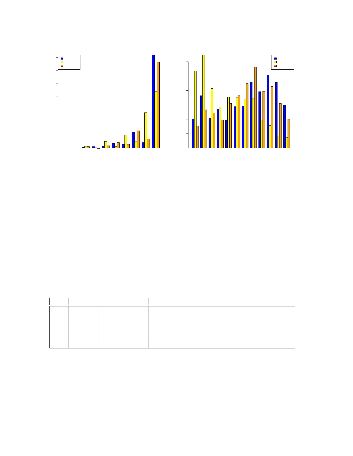
F rom Chain-Ladder to Individual Claims Reserving Ronald Ric hman ∗ Mario V. W ¨ uthric h † Revised V ersion of F ebruary 19, 2026 Abstract The chain-ladder (CL) method is the most widely used claims reserving technique in non-life insurance. This man uscript introduces a nov el approac h to computing the CL reserves based on a fundamen tal restructuring of the data utilization for the CL prediction pro cedure. Instead of rolling forw ard the cumulativ e claims with estimated CL factors, we estimate m ulti-p erio d factors that pro ject the latest observ ations directly to the ultimate claims. This alternativ e persp ective on CL reserving creates a natural path wa y for the application of machine learning techniques to individual claims reserving. As a pro of of concept, we presen t a small-scale real data application emplo ying neural net works for individual claims reserving. Keyw ords. Claims reserving, c hain-ladder metho d, individual claims reserving, micro-level reserving, granular reserving, neural netw orks, Mack’s metho d. 0 Addendum After uploading the first version of this man uscript to arXiv , Florian Gerhardt (thank y ou v ery muc h!) p oin ted out that our main result had already b een established on page 130 of Lorenz–Sc hmidt [13], where the approach is referred to as the grossing up metho d. F ollo wing the theorem in that reference, the authors remark that “..., the grossing up metho d is irrelev ant in practice.” W e believe that this assessment is to o p essimistic in the era of mac hine learning. In our view, precisely this structural p ersp ective may pro vide the k ey to bringing individual claims reserving into practical application. F or this reason, we ha ve c hosen to leav e the pap er essen tially unc hanged, in the hope of con vincing the reader that this approac h offers a promising direction for future researc h. 1 In tro duction Ab out a decade ago, research of individual claims reserving utilizing mac hine learning (ML) tec hniques b egan to emerge. Since then, numerous methods and mo dels ha v e b een prop osed, including regression trees, gradient bo osting machines, and neural netw orks. Nevertheless, the area of individual claims reserving remains predominantly a research domain and has not y et ac hiev ed a widespread adoption in industry practice. Schneider–Sc hw ab [18] write: “Typically , ∗ insureAI, ronaldric hman@gmail.com † Departmen t of Mathematics, ETH Zurich, mario.wuethric h@math.ethz.ch 1 new er models which consider ric her data on individual claims are either parametric or use mac hine learning tec hniques. Ho w ever, none ha ve b ecome a gold standard, and adv ances are still needed.” W e attribute this fact to v arious challenges. First, it is difficult to find publicly av ailable individual claims data. This clearly hinders researc h in this area of actuarial science. Second, individual claims data is censored, lo w-frequency and of a complex time-series structure. It is generally difficult to build goo d predictiv e models for suc h problems. Third, the claims reserving problem is a multi-perio d forecasting problem. Ho w ev er, often, the underlying algorithms are only trained for performing one-p erio d ahead forecasts. Naturally , a t weak is required to work around this problem going from one- to multi-perio d forecasts. F ourth, the implemen tation and structure of the prop osed individual claims reserving metho ds is rather complex and often sp ecific to a certain claims reserving situation, for instance, every insurance compan y collects historic data of a sligh tly differen t nature (and format). This mak es it difficult to benchmark the differen t methods. Moreov er, the proposed approac hes often need extended h yp er-parameter tuning, e.g., to a void biases, this leav es the question op en whether the prop osed method easily generalizes to other claims reserving situations (in a broader sense). This pap er introduces a fundamentally nov el approac h whic h w e en vision as a transformative step tow ard the widespread adoption of individual claims reserving across the insurance indus- try . This transformative step is not ab out a sp ecific ML arc hitecture, but our core idea is to reorganize historical individual claims data for direct m ulti-p erio d forecasting. The main step is to reformulate the foundational chain-ladder (CL) reserving algorithm so that one can p erform m ulti-p erio d model fitting and forecasting. Once this step is fully understo o d, adapting this idea to ML metho ds is straigh tforward. W e will explain this in detail, after outlining the presen t state of the field of individual claims reserving using ML metho ds. W e observ e four main techniques to cope with the multi-perio d forecasting problem in individual claims reserving: (1) The m ulti-p erio d forecasting is p erformed b y a recursive one-perio d forecast pro cedure using past observ ations as inputs. Rolling this recursive procedure into the future, missing observ ed inputs are replaced b y their forecasts. This is the first and most p opular metho d used for m ulti- p erio d forecasting; for literature in individual claims reserving see, e.g., De F elice–Moriconi [5] and Chaoubi et al. [4]. W e briefly explain why this pro cedure may b e problematic. Consider observ ations ( Y 1 , . . . , Y t ) to forecast a next resp onse Y t +1 at time t ≥ 1. The natural forecast is giv en by ( Y 1 , . . . , Y t ) 7→ b Y t +1 := E [ Y t +1 | Y 1 , . . . , Y t ] . One p eriod later, at time t + 1, we hav e collected observ ations ( Y 1 , . . . , Y t +1 ) and w e build the next forecast of resp onse Y t +1 b y ( Y 1 , . . . , Y t +1 ) 7→ b Y t +2 = E [ Y t +2 | Y 1 , . . . , Y t +1 ] . (1.1) This gives a natural recursive one-p erio d ahead forecast algorithm. The main difficult y in applying it in practice is that the observ ation Y t +1 is not av ailable at time t , and we cannot roll this algorithm into the future. The simple solution to this problem is to impute the prediction b Y t +1 for the missing observ ation Y t +1 , that is, w e set ( Y 1 , . . . , Y t , b Y t +1 ) 7→ b Y † t +2 := E h Y t +2    Y 1 , . . . , Y t , b Y t +1 i . (1.2) 2 Ho w ev er, in general, this prop osal of m ulti-p erio d forecasting is inappropriate. W e giv e an example. Assume that all resp onses are binary , Y t ∈ { 0 , 1 } , t ≥ 1. Thus, the conditional exp ectation in (1.1) is based on binary observ ations ( Y 1 , . . . , Y t , Y t +1 ) ∈ { 0 , 1 } t +1 , and so is the ML mo del that is trained to approximate the forecast (1.1). Ho w ev er, the forecast b Y t +1 ∈ [0 , 1] imputed in (1.2) can take any value in the unit interv al, e.g., b Y t +1 = 0 . 46, and the forecast mo del (1.1) do es not kno w how to deal with this input v alue, because it has never seen a v alue differen t from zero or one before (because it only learned to deal with binary inputs). (2) A w ork around of the problem discussed in item (1) is to learn a full simulation model from whic h one can sim ulate Y t +1 , giv en Y 1 , . . . , Y t . This then allo ws one to p erform a Mon te Carlo sim ulation extrap olation. This is the solution applied, e.g., in W ¨ uthric h [21] and Delong et al. [6]. The main disadv an tage of this approac h clearly is that w e need an accurate simulation mo del. If the responses Y t con tain, e.g., claims paymen ts, claims incurred and other sto c hastic pro cesses, this is clearly b eyond our mo deling capabilities. (3) The works of Kuo [9, 10] present sequence-to-sequence forecasting methods, and the approac h presen ted b y Gabrielli [7] uses a rather similar tec hnique. These approac hes mask missing obser- v ations, and the predictive mo del learns to p erform forecasting under incomplete information, e.g., it tries to directly predict Y t +2 , giv en ( Y 1 , . . . , Y t ), b y learning from all available information. This is a very suitable proposal. In practical applications, the main difficulty of this approac h lies in controlling and mitigating p otential biases during mo del training. Our prop osal p ossesses this problem too, but w e will see that exp ert in terven tion is rather easy in our approach. (4) Finally , an other option is to directly predict the ultimate claims from the av ailable infor- mation. There are t w o approaches in the literature that consider this option. The first one is related to surviv al analysis that properly accounts for censored information. This has b een considered, e.g., in Lop ez et al. [12, 11], Bladt–Pittarello [2], Hiabu et al. [8] or T urcotte–Shi [20]. The second metho d of a direct ultimate claim prediction uses reinforcement learning to optimally up date the forecast based on the incoming information; see Av anzi et al. [1] Our prop osal aligns with option (4) of directly forecasting the ultimate claims, but the con- struction of our ultimate claim predictor is rather differen t from the tw o prop osals ab ov e. Our starting p oin t is the classic CL metho d. Usually , the CL method is rather accurate on aggregate claims – verified by its successful use o v er man y decades – and the CL metho d is v ery simple in its use, not very prone to biases, easy to handle and easy to manipulate by exp ert knowl- edge. Our main con tribution is to restructure the estimation of the CL factors. This reshap es the estimation procedure such that it can naturally be extended to ML metho ds on individual claims. Thus, our contribution is this nov el representation of the CL estimation and not the ML metho d itself. In fact, to k eep things simple w e select an elementary neural net work architecture in our example. W e b elieve that our prop osal widely op ens the do or for a natural pathw ay of ML applications to individual claims reserving. A few immediate adv an tageous o v er the exist- ing methods are the following: (i) Our prop osal can deal with any sort of stochastic dynamic co v ariates suc h as claims incurred or m ultiple pa yment pro cesses of sev eral injured people. (ii) It is a natural next step b ey ond the CL algorithm. This means that the basis is the CL metho d and our approac h can easily b e regularized using the CL predictor to con trol for biases. (iii) It can easily be extended to cash-flo w forecasting in the sense of sequence-to-sequence metho ds as stated in item (3) ab ov e. In summary , the main adv antage of starting from a CL structure is 3 that the CL results give the guardrails for the ML predictions. A limitation that we should men tion is that our prop osal only considers rep orted but not settled (RBNS) claims. This is common to most researc h in individual claims reserving, i.e., claims need to b e rep orted so that their individual claims history is a v ailable for the use of the prediction of their further developmen t. Incurred but not rep orted (IBNR) claims need to b e forecast in addition, e.g., b y a suitable frequency-severit y reserving mo del. Organization of the man uscript. In Section 2, w e revisit Mack’s CL mo del [14], and we presen t our main tec hnical results that giv es an alternative v ersion of estimating the CL reserves. Section 3 takes this alternative version to present a natural extension to individual claims re- serving. In Section 4, w e study tw o small-scale real data examples that serve as pro of of concept of our prop osal. Finally , in Section 5 we conclude and w e give a list of next steps to lift this prop osal to its full p o w er for individual claims reserving. The mathematical pro ofs are given in the app endix. 2 Chain-ladder metho d 2.1 Mac k’s distribution-free c hain-ladder mo del W e start b y revisiting Mac k’s distribution-free CL mo del [14]. Denote cum ulativ e pa ymen ts for claims in accident perio d i ∈ { 1 , . . . , I } and with dev elopmen t delay j ∈ { 0 , . . . , J } by C i,j , and assume that these cum ulative pa yments are strictly positive for all pairs ( i, j ). Assume I > J , i.e., at least one accident p erio d is fully observ ed (dev elop ed), and the goal is to predict the ultimate claims C i,J of accident p eriods i > I − J at time I . Mo del Assumptions 2.1 (CL mo del) The cumulative p ayment pr o c esses ( C i,j ) 0 ≤ j ≤ J of dif- fer ent ac cident p erio ds i ∈ { 1 , . . . , I } ar e indep endent. Ther e exist p ositive p ar ameters ( f j ) J − 1 j =0 and ( σ 2 j ) J − 1 j =0 such that for al l i ∈ { 1 , . . . , I } and j ∈ { 0 , . . . , J − 1 } the fol lowing holds E [ C i,j +1 | C i, 0 , . . . , C i,j ] = f j C i,j , V ar ( C i,j +1 | C i, 0 , . . . , C i,j ) = σ 2 j C i,j . An easy consequence of these assumptions is that one can compute the conditionally exp ected ultimate claims C i,J of accident p eriods i > I − J at time I as follows E [ C i,J | C i, 0 , . . . , C i,I − i ] = C i,I − i J − 1 Y l = I − i f l , (2.1) where C i, 0 , . . . , C i,I − i are the cum ulativ e pa yments of accident p erio d i that are observ ed at time I , i.e., the cumulativ e pa ymen ts C i,j with indices i + j ≤ I . This reflects the observed upp er triangle 1 at time I . 1 The shap e of the observed cumulativ e pa yments ( C i,j ) i + j ≤ I , is a triangle for I = J + 1 and it is a trap ezoid for I > J + 1. T o simplify language we generally speak ab out triangles, ev en if the shape is a trap ezoid. This is common practice in claims reserving. 4 T o apply the CL method for reserving, there remains the estimation of the (unknown) CL factors ( f j ) J − 1 j =0 . A t time I , these CL factors are commonly estimated by b f j = P I − j − 1 i =1 C i,j +1 P I − j − 1 i =1 C i,j . (2.2) This motiv ates the CL pr e dictors for acciden t perio ds i > I − J at time I b C i,J = C i,I − i J − 1 Y l = I − i b f l . (2.3) This is the classic CL predictor. It is unbiased for the (conditionally) exp ected ultimate claim; see Mack [14] and W ¨ uthrich–Merz [23, Lemma 3.3]. W e next give a different representation of the CL predictor b C i,J , i > I − J , and this will pav e the w ay to individual claims reserving utilizing ML tec hniques. 2.2 Recursiv e chain-ladder factor estimation W e can in terpret the prediction in (2.3) as a forw ard-path estimation of the conditionally ex- p ected ultimate claim (2.1). This can b e seen as follows b C i,J = C i,I − i J − 1 Y l = I − i b f l = C i,I − i · b f I − i | {z } I − i → I − i +1 · b f I − i +1 | {z } I − i → I − i +2 · . . . · b f J − 1 . Th us, this is a step-wise (one-p erio d ahead) roll forw ard extrap olation of C i,I − i using the CL factor estimates ( b f l ) J − 1 l = I − i – this is precisely the meaning of chain-ladder extrap olation, see Figure 1. Figure 1: Step-wise roll forw ard (chain-ladder) extrap olation to predict the ultimate claims C i,J using observ ations C i,I − i , i > I − J , at time I (for I = 7 and J = 6). W e no w giv e a differen t, recursiv e v ersion that pro vides us with the same CL predictor by p erforming a one-shot ultimate pr e diction . Define the pr oje ction-to-ultimate (PtU) factors as follo ws F j := J − 1 Y l = j f l for j ∈ { 0 , . . . , J − 1 } . 5 Naturally , the follo wing iden tity holds E [ C i,J | C i, 0 , . . . , C i,I − i ] = C i,I − i J − 1 Y l = I − i f l = C i,I − i F I − i . The no vel approach that we prop ose is to directly estimate these PtU factors ( F j ) J − 1 j =0 . F or this, w e b egin b y in tro ducing a new notation for the ultimate claims that are fully observed at time I , this will simplify the notation in the recursion b elow. Set b C ∗ i,J = C i,J for all i ∈ { 1 , . . . , I − J } . W e emphasize that these v ariables are all observ ed at time I ; they corresp ond to the fully dev elop ed accident p eriods at time I . (a) Initialization. W e p erform the estimation pro cedure of the PtU factors ( F j ) J − 1 j =0 recursiv ely starting from the upper-right corner of the claims reserving triangle. W e estimate the PtU factor of the last dev elopmen t p erio d j = J − 1 b y b F J − 1 = b f J − 1 = P I − J i =1 b C ∗ i,J P I − J i =1 C i,J − 1 and b C ∗ I − J +1 ,J = C I − J +1 ,J − 1 b F J − 1 . (2.4) (b) Iter ation. The estimation is extrap olated recursively from j + 1 → j by setting b F j = P I − j − 1 i =1 b C ∗ i,J P I − j − 1 i =1 C i,j and b C ∗ I − j,J = C I − j,j b F j , (2.5) for j ∈ { 0 , . . . , J − 2 } . Figure 2: Bac kward extrap olation to predict the ultimate claims C i,J , i > I − J , using the estimated PtU factor estimates ( b F j ) J − 1 j =0 : (left-middle-righ t) corresp ond to j = J − 1 = 5, j = 4 and j = 3. The estimation of the forecast pro cess (2.4)-(2.5) starts in the upp er-righ t corner of the claims reserving triangle j = J − 1, see Figure 2. Then it mov es recursiv ely j + 1 → j along the last observ ed diagonal to the most recent accident perio d i = I ( j = 0) by dir e ctly predicting the ultimate claims using (2.5). Prop osition 2.2 b C ∗ i,J = b C i,J for al l ac cident p erio ds i ∈ { I − J + 1 , . . . , I } . 6 The pro of of this prop osition is given in the app endix, and this is the result pro ved in Lorenz– Sc hmidt [13]. The exciting fact stated in Prop osition 2.2 is that b oth algorithms – the step-wise roll forw ard CL extrapolation of Figure 1 and the backw ard extrapolation of Figure 2 – lead to the iden tical CL reserves. W e giv e some remarks. • Both algorithms shown in Figures 1 and 2 use the identical information and they provide the iden tical forecasts. W e can view this as an optimal use of triangular information b e- cause every observed cum ulativ e paymen t C i,j , i + j ≤ I , is used whenev er it is appropriate. This is differen t, e.g., from the bo otstrap of individual claims histories of Rosenlund [17] who bases his mo del learning pro cedure only on claims with fully observed tra jectories. • The claims reserving problem is a t ypical situation of censored observ ations, with the additional difficulty that differen t (censored) observ ations hav e differen t maturity . This giv es the close connection to surviv al analysis. W e mention the Kaplan–Meier weigh ting metho d considered in Lop ez et al. [12, 11] to correct for censored claims information, although the method in these references is not directly applicable to claims reserving b ecause cum ulative claims pa yments are assumed to b e prop ortional to time to settlemen t. Other surviv al analysis pap ers of a similar nature are Hiabu et al. [8] – this paper considers surviv al analysis for IBNR prediction using a CL forw ard path – and Bladt–Pittarello [2] use the Aalen–Johansen estimator in a m ulti-state pro cess on a finite state space. 2.3 Chain-ladder RBNS reserving The ultimate claim predictions b C i,J of the CL algorithm co ver b oth the RBNS and the IBNR claims. Our first mo dification is to only predict ultimates of RBNS claims at time I ; by RBNS claim w e denote an y rep orted claim at time I which can either be a closed or an open one (i.e., w e allo w for re-openings in this definition). W e lab el individual claims by ν , separately for each o ccurrence p erio d i ∈ { 1 , . . . , I } . Let C i,j | ν denote the cum ulativ e pa yments of the ν -th claim of occurrence p erio d i after developmen t perio d j (since o ccurrence). W e can then write for the aggregate cumulativ e paymen ts C i,j = X ν : T i | ν ≤ j C i,j | ν , where the sum runs ov er all claims ν of accident p erio d i that are rep orted at time i + j , and T i | ν ∈ { 0 , . . . , J } denotes the rep orting delay of the ν -th claim of accident p erio d i . The rep orted claims at time I are c haracterized by i + T i | ν ≤ I and the IBNR claims b y i + T i | ν > I . W e no w fo cus on RBNS reserves that only inv olve rep orted claims. F or this w e define a version of the PtU factor estimates ( b F ( r ) j ) J − 1 j =0 that only consider the rep orted claims in the corresp onding p erio ds. (a) Initialization. W e set b C ( r ) i,J | ν = C i,J | ν for all claims ν with acciden t dates i ≤ I − J ; these claims are fully dev elop ed. W e then initialize for j = J − 1 b F ( r ) J − 1 = P I − J i =1 P ν : T i | ν ≤ J − 1 b C ( r ) i,J | ν P I − J i =1 P ν : T i | ν ≤ J − 1 C i,J − 1 | ν and b C ( r ) I − J +1 ,J | ν = C I − J +1 ,J − 1 | ν b F ( r ) J − 1 , (2.6) 7 for all rep orted claims ν of acciden t p erio d I − J + 1, i.e., with reporting delay T I − J +1 | ν ≤ J − 1. The PtU factor estimate b F ( r ) J − 1 only considers claims that hav e a reporting dela y less or equal to J − 1, th us, in the n umerator and the nominator of the PtU factor estimate b F ( r ) J − 1 w e consider the identic al c ohort of rep orted claims. Thus, this is a consisten t consideration of rep orted claims extrap olation. (b) Iter ation. This is recursiv ely extended from j + 1 → j ∈ { 0 , . . . , J − 2 } by setting b F ( r ) j = P I − j − 1 i =1 P ν : T i | ν ≤ j b C ( r ) i,J | ν P I − j − 1 i =1 P ν : T i | ν ≤ j C i,j | ν and b C ( r ) I − j,J | ν = C I − j,j | ν b F ( r ) j , (2.7) for all rep orted claims ν of acciden t p erio d I − j , i.e., with rep orting dela y T I − j | ν ≤ j . Again, in the numerator and the nominator of the PtU factor estimate b F ( r ) J − 1 w e consider the identic al c ohort of rep orted claims ν , i.e., with T i | ν ≤ j . W e can also interpret this of having a moving target X ν : T i | ν ≤ j b C ( r ) i,J | ν , in the numerators of (2.7) as this claims cohort is decreasing for decreasing j due increasingly man y IBNR claims T i | ν > j for decreasing j . W e would like to highlight the similarity of our proposal to Schnieper’s mo del [19], although the estimation procedures differ. Schnieper’s mo del separates RBNS from IBNR claims similarly to our PtU estimation, but Sc hniep er’s estimation of the dev elopment factors contains reserves for IBNR claims (once they are rep orted), whereas our estimation pro cedure (2.7) fixes the claims cohort and pro jects it directly to its ultimates b C ( r ) i,J | ν without including reserves for additional late rep orted claims. 3 Individual ultimate prediction using mac hine learning The recursiv e form ulas (2.6)-(2.7) give the intuition for ho w the CL metho d can b e extended to an individual claims ML metho d using any a v ailable input information. Denote the settlement pro cess of claim ν of acciden t p erio d i b y C i | ν := ( C i,l | ν , X i,l | ν ) J l =0 , where ( X i,l | ν ) J l =0 can b e any claims feature process that ma y inv olve static c ovariates that are known at rep orting (like claim t yp e or business line), deterministic dynamic c ovariates (like settlement dela y) and sto chastic dynamic c ovariates (like claims incurred pro cess or claim status pro cess for op en/closed claims). W e emphasize that this latter information typically is not fully kno wn at time I for RBNS claims with accident dates i > I − J as it sto chastically ev olves in to the future, and one may wan t to consider its sto chastic mo deling and prediction as w ell. The exciting fact ab out our metho d presen ted b elow is that extrap olation of the claims feature pro cess is not necessary! 3.1 Recursiv e individual claims reserving Assumption. W e assume that the individual claims pro cesses C i | ν are indep endent, and that they are conditionally i.i.d., given the static cov ariates kno wn at reporting. T o comply with the previous assumption it may require to adjust some of the dynamic quantities with inflation indices (e.g., pa yments, incurred and case reserves). F or late rep orted RBNS 8 claims, we mask the co v ariate pro cess part of ( X i,l | ν ) J l =0 that refers to time p erio ds j < T i | ν b efore rep orting. W e no w presen t a recursiv e forecast pro cedure for individual claims that in its metho dology is equiv alen t to (2.6)-(2.7). (a) Initialization. W e start with acciden t p erio d I − J + 1 or, equiv alen tly , dev elopment perio d j = J − 1. F or all claims ν that ha ve o ccurred in accident p erio ds i ≤ I − J , the sto chastic pro cesses C i | ν = ( C i,l | ν , X i,l | ν ) J l =0 are fully observed, and we aim at predicting the ultimates C I − ( J − 1) ,J | ν of all claims in the next accident p erio d I − J + 1. These claims are reported at time I , th us, they ha v e rep orting delay T I − ( J − 1) | ν ≤ J − 1, and we ha ve observ ed their claims histories ( C I − ( J − 1) ,l | ν , X I − ( J − 1) ,l | ν ) J − 1 l =0 . T o bring the learning data into the same shap e, we are only allow ed to consider those claims that ha ve been rep orted b efore settlemen t delay J . This giv es us the learning data to perform the initial learning step L J − 1 = n C i,J | ν , ( C i,l | ν , X i,l | ν ) J − 1 l =0  ; i ≤ I − J and T i | ν ≤ J − 1 o . Based on this learning data L J − 1 , we build the regression function ( C i,l | ν , X i,l | ν ) J − 1 l =0 7→ µ J − 1  ( C i,l | ν , X i,l | ν ) J − 1 l =0  = E h C i,J | ν    ( C i,l | ν , X i,l | ν ) J − 1 l =0 i . (3.1) This regression function µ J − 1 ( · ) describes the forecast step J − 1 → J , and it allows us to predict the ultimates for the claims ν of accident p erio d i = I − J + 1, with observed claims histories ( C I − J +1 ,l | ν , X I − J +1 ,l | ν ) J − 1 l =0 . In particular, we can compute the forecast (assuming stationary along the occurrence perio d axis i ) b C I − ( J − 1) ,J | ν := µ J − 1  ( C I − ( J − 1) ,l | ν , X I − ( J − 1) ,l | ν ) J − 1 l =0  = E h C I − ( J − 1) ,J | ν    ( C I − ( J − 1) ,l | ν , X I − ( J − 1) ,l | ν ) J − 1 l =0 i . W e app end these predictions to the observ ed claims histories for accident p erio d I − J + 1 b C I − ( J − 1) | ν :=  ( C I − ( J − 1) ,l | ν , X I − ( J − 1) ,l | ν ) J − 1 l =0 , b C I − ( J − 1) ,J | ν  . (3.2) This initializes the recursion, and it reflects the figure on the left-hand side of Figure 2. (b) Iter ation. W e recursively extend this from j + 1 → j ∈ { 0 , . . . , J − 2 } or, equiv alently , to acciden t p eriod I − j . The sto chastic pro cesses C i | ν are fully observ ed for accident p erio ds i ≤ I − J , and for acciden t p erio ds I − ( J − 1) ≤ i ≤ I − ( j + 1), w e hav e partially observ ed claims histories b C i | ν including an app ended ultimate claim forecast b C i,J | ν . The goal is to extend this to the claims ν of acciden t perio d I − j , whic h ha v e a rep orting dela y T I − j | ν ≤ j and observed claims histories ( C I − j,l | ν , X I − j,l | ν ) j l =0 at time I . W e select the learning dataset suc h that it aligns with the maximal reporting lag of the RBNS claims of acciden t perio d I − j at time I to build consisten t claims cohorts L j = n C i,J | ν , ( C i,l | ν , X i,l | ν ) j l =0  ; i ≤ I − J and T i | ν ≤ j o ∪ n b C i,J | ν , ( C i,l | ν , X i,l | ν ) j l =0  ; I − ( J − 1) ≤ i ≤ I − ( j + 1) and T i | ν ≤ j o . (3.3) 9 Based on this learning data L J − 1 , we build the regression function, whic h for the fully dev elop ed claims of acciden t perio ds i ≤ I − J considers ( C i,l | ν , X i,l | ν ) j l =0 7→ µ j  ( C i,l | ν , X i,l | ν ) j l =0  = E h C i,J | ν    ( C i,l | ν , X i,l | ν ) j l =0 i , (3.4) this predicts from developmen t p erio d j → J . F or the claims of acciden t p erio ds I − ( J − 1) ≤ i ≤ I − ( j + 1) we use the mo dified v ersion ( C i,l | ν , X i,l | ν ) j l =0 7→ µ j  ( C i,l | ν , X i,l | ν ) j l =0  = E h C i,J | ν    ( C i,l | ν , X i,l | ν ) j l =0 i = E h b C i,J | ν    ( C i,l | ν , X i,l | ν ) j l =0 i , (3.5) the last step uses the to w er property of conditional exp ectation. The latter can b e learned from the second line of the learning sample L j giv en in (3.3). Using this learned regression function µ j ( · ), given in (3.4)-(3.5), we forecast the ultimate claims of acciden t perio d I − j b y b C I − j,J | ν := µ j  ( C I − j,l | ν , X I − j,l | ν ) j l =0  = E h C I − j,J | ν    ( C I − j,l | ν , X I − j,l | ν ) j l =0 i . This ultimate claim forecast is appended to the av ailable claims histories b C I − j | ν :=  ( C I − j,l | ν , X I − j,l | ν ) j l =0 , b C I − j,J | ν  . (3.6) Recursiv e iteration completes the ultimate claim forecasting, precisely reflecting the philosophy of Section 2.2. This is illustrated by the middle and the right-hand side figures of Figure 2. Remarks 3.1 • Crucially , the ab o ve algorithm can deal with any dynamic sto c hastic co v ariates without their extrap olation. • The abov e algorithm is not ab out a certain ML arc hitecture, but it is rather ab out ho w the data is organized to p erform the one-shot ultimate prediction. The input ( X i,l | ν ) j l =0 can b e of any (reasonable) form, it can include sto c hastic dynamic cov ariates, it can inv olve textual data lik e medical rep orts, but it can also include information at a higher time frequency , i.e., the forecasting frequency p erio ds j ≥ 0 can also deal with contin uously arriving information ( X i,l | ν ) l ∈ [0 ,j ] . At this stage the choice of the ML architecture will b ecome imp ortant as it needs to b e able to deal with the formats of the inputs. • In practical applications, the only critical item of this algorithm is its recursive nature. In (3.2) and (3.6) we app end the estimated ultimate claim of a giv en acciden t p erio d i = I − ( j + 1) to the observ ations, in order to b e able to learn the one of the next accident p erio d i + 1 = I − j . This recursiv e nature has the disadv antage that if one accident p erio d has a biased estimate, this bias will propagate through the follo wing acciden t perio d estimates. Therefore, it is v ery imp ortant to correct for biases whenev er p ossible. • This recursive algorithm uses the observed data in the same efficien t wa y as the CL metho d, this is motiv ated by the result of Prop osition 2.2. In particular, w e simultaneously learn from fully developed but also from non-settled claims, such that alw ays all relev an t infor- mation is considered for prediction. The trade-off of this optimal use of information is the bias-con trol mentioned in the previous item. 10 4 Real data examples W e presen t t w o small scale real data examples. The first one considers acciden t insurance and the second one liability insurance. These t wo examples serv e as a pro of of concept, and they are neither mean t to solve the most complex claims reserving problem, nor do they use the latest most fancy ML techniques, see second item of Remarks 3.1. As mentioned, our main con tribution is the optimal use of triangular data for one-shot ultimate claim prediction which leads to our key result of Prop osition 2.2. This widely op ens the do or for individual claims reserving, and in our final Section 5, b elow, w e highligh t potential next steps. T o further strengthen our prop osal, w e select t w o examples for which also the low er triangle is kno wn. This allo ws us to b enc hmark our forecasts against the true outcomes. Naturally , this requires that w e restrict ourselv es to older acciden t p erio ds as the most recent accident perio d considered needs to b e fully developed to b e able to b enc hmark it against the ground truth. 4.1 Description of data 4.1.1 Acciden t insurance data W e use an acciden t insurance dataset on an annual scale with 5 fully observed acciden t y ears, i.e., w e hav e a fully observed 5 × 5 square. F or mo del fitting and forecasting, w e only use the upp er triangle , as in Figure 2, and w e benchmark the forecasts against the true ultimates whic h are av ailable here (having also observ ed the lo wer triangle). Characteristic Time scale calendar y ears Num b er of accident years 5 Num b er of developmen t years 5 Num b er of rep orted claims 66,639 Data description Ann ual individual cumulativ e paymen ts C i,j | ν Claim status O i,j | ν ∈ { 0 , 1 } for closed/op en Binary static cov ariate for work or leisure acciden t Calendar mon th of accident Rep orting delay in daily units T able 1: Characteristics of acciden t dataset. T able 1 shows the av ailable data of the accident insurance dataset. There are 66,639 rep orted claims with a fully observed developmen t history ov er the 5 × 5 square. Besides the individ- ual cumulativ e pa ymen t pro cess ( C i,j | ν ) j , there is information ab out the claim status pro cess ( O i,j | ν ) j , with O i,j | ν = 1 meaning that the ν -th claim of accident year i is op en at the end of settlemen t dela y j , and closed otherwise. Then, there is static information ab out: w ork or leisure related accident, the calendar month of the accident and the rep orting delay in daily units. W e collect all this static and dynamic co v ariate information in the claims feature pro cess ( X i,j | ν ) j , see Section 3. W e giv e some remarks on the a v ailable co v ariates. The claim status pro cess ( O i,j | ν ) j is stochastic dynamic. T ypically , for closed claims O i,j | ν = 0 we do not exp ect further pa ymen ts b eyond settlemen t dela y j and the cumulativ e pa yment pro cess should remain constant in these further 11 p erio ds. Ho w ever, claims can b e re-op ened for further (unexp ected) claims developmen ts. Our metho d also reserves for these (potential) pa ymen ts. Typically , work or leisure related acciden ts are differen t, e.g., a bank employ ee cannot ha ve a skiing accident during work hours. The calendar mon th will distinguish summer from win ter activities (biking vs. skiing acciden ts). Finally , the rep orting delay is imp ortan t to infer the w aiting perio d of the insurance contract, e.g., if the con tract has a waiting perio d of 3 months, then daily allow ance is only paid after this w aiting p erio d. Typically , the waiting perio d is p ositiv ely correlated with the rep orting delay . 4.1.2 Liabilit y insurance data The second dataset considers liability insurance (excluding motor liability). W e again ha ve a fully observed 5 × 5 square and for mo del fitting w e only use the upp er triangle. Characteristic Time scale calendar years Num b er of accident years 5 Num b er of developmen t years 5 Num b er of rep orted claims 21,991 Data description Ann ual individual cumulativ e paymen ts C i,j | ν Claim status O i,j | ν ∈ { 0 , 1 } for closed/op en Claim incurred I i,j | ν ≥ 0 Binary static cov ariate for priv ate vs. commercial liability Calendar month of accident Rep orting delay in daily units T able 2: Characteristics of liabilit y dataset. T able 2 shows the a v ailable data of the liability insurance dataset. The main difference to the previous example is that for this dataset there is also a claims incurred pro cess ( I i,j | ν ) j a v ailable. The claims incurred pro cess is a claims adjuster’s prediction of the individual ultimate claim that is constantly up dated when new information b ecomes av ailable, i.e., this is a sto chastic pro cess driv en by the claims adjuster’s assessmen ts. Additionally , there is the case reserv e pro cess ( R i,j | ν ) j a v ailable by computing R i,j | ν = I i,j | ν − C i,j | ν . 4.2 F orecast mo del 4.2.1 Net work architecture Next, we select the regression functions ( µ j ) J − 1 j =0 ; w e refer to (3.1) and (3.4)-(3.5). In our t wo small scale examples w e hav e I = 5 and J = 4, th us, w e only need 4 regression functions ( µ j ) 3 j =0 in each of the tw o examples. W e giv e a crude prop osal that clearly allows for mo dification and impro v emen t for bigger and refined datasets, see also Remarks 3.1 and the discussion in Section 5. Namely , we mo del all 4 regression functions ( µ j ) 3 j =0 b y separate net w orks. Hence, we ha v e to learn 4 differen t net works for eac h of the t wo examples. Another simplification that w e mak e is the follo wing Mark ov assumption µ j  ( C i,l | ν , X i,l | ν ) j l =0  = µ j  C i,j | ν , X i,j | ν  . (4.1) 12 That is, w e do not consider the entire individual claims history ( C i,l | ν , X i,l | ν ) j l =0 , but w e assume that it is sufficien t to kno w the last state ( C i,j | ν , X i,j | ν ). A natural choice for µ j under the Marko v assumption (4.1) is a feed-forw ard neural net work (FNN) architecture; w e will use the FNN notation and terminology of W ¨ uthric h–Merz [24], and for a broader introduction to net works we also refer to that reference. If the Mark ov assumption (4.1) fails to hold, then a natural candidate for µ j is a T ransformer arc hitecture with an in tegrated CLS tok en for input enco ding; see Ric hman et al. [15]. Mo dule Dimension # W eights Activ ation Input la yer 5 – – 1st hidden lay er 20 120 tanh 2nd hidden lay er 15 315 tanh 3rd hidden lay er 10 160 tanh Output la yer 1 11 exp T able 3: Selected FNN arc hitecture µ FNN j , for 1 ≤ j ≤ J − 1, in the accident insurance example. W e select iden tical plain-v anilla FNN architectures ( C i,j | ν , X i,j | ν ) 7→ µ FNN j ( C i,j | ν , X i,j | ν ) = exp  z (3:1) j ( C i,j | ν , X i,j | ν )  , for all dev elopment p erio ds j = 0 , . . . , 3. These FNN arc hitectures µ FNN j consider FNNs z (3:1) j with 3 hidden lay ers with n umber of neurons giv en b y (20 , 15 , 10) in the 3 hidden lay ers. The explicit sp ecifications are shown in T able 3, and this results in FNNs with 606 weigh ts to b e fitted in the case of the accident insurance dataset for ev ery j = 0 , . . . , 3. Since under the Mark o v assumption (4.1), the input has alwa ys the same dimension, w e use the iden tical FNN arc hitecture for all regression functions ( µ FNN j ) 3 j =0 , only their w eigh ts will differ (after mo del fitting). F or an explicit implementation of this architecture we refer to W ¨ uthric h–Merz [24, Listing 7.1], only the part inv olving the volume in that reference needs to b e dropp ed b ecause here we only hav e unit exposures. W e select the same FNN arc hitecture also for the liabilit y insurance dataset. In this second dataset we ha v e an input dimension of 7 (additionally considering claims incurred and case reserv es). This results in 160 w eigh ts in the first hidden lay er and a FNN arc hitecture of totally ha ving 646 w eights. 4.2.2 Data pre-pro cessing and mo del fitting W e are almost ready now to fit these four FNNs ( µ FNN j ) 3 j =0 for b oth examples. There remains the input pre-pro cessing and the selection of the fitting pro cedure. T ypically , inputs ( C i,j | ν , X i,j | ν ) should b e standardized to receive an efficient sto chastic gradien t descent (SGD) fitting pro cedure. The individual cumulativ e pa ymen ts are considered on the log-scale and they are standardized b y e C i,j | ν ← log  max { 1 , C i,j | ν }  − b m b s . where b m and b s are the empirical mean and standard deviation of log (max { 1 , C i,j | ν } ) ov er all available cumulativ e pa ymen ts C i,j | ν sim ultaneously in all acciden t y ears i , for all claims ν and in all dev elopment p eriods j . 13 In the case of the liability dataset, we apply the same transformation to claims incurred I i,j | ν , and we apply the standardization to the case reserv es R i,j | ν without going to the log-scale. F urthermore, the claim status O i,j | ν ∈ { 0 , 1 } does not require pre-pro cessing. The binary static co v ariates are mapp ed to { 0 , 1 } , the calendar mon th cm ∈ { 1 , . . . , 12 } is scaled to [0 , 1] b y transforming it to ( cm − 1) / 11, and the rep orting delay is censored at 365 da ys, mapp ed to the log-scale and b eing scaled to [0 , 1] as for the calender month. This provides us with the pre-pro cessed input ( e C i,j | ν , f X i,j | ν ) which is used to forecast the corresp onding ultimate claim ( e C i,j | ν , f X i,j | ν ) 7→ b C FNN i,J | ν = µ FNN j  e C i,j | ν , f X i,j | ν  . These FNN regression functions are learned recursiv ely as describ ed in Section 3, see also Figure 2. F or fitting, w e apply the SGD algorithm with early stopping using the hyper-parameter sp ecification as rep orted in T able 4. Comp onen t Setting Loss function mean squared error (MSE) Optimizer Adam with learning rate 10 − 3 Batc h size and ep ochs 4,096 and 1,000 Learning-v alidation split 9 : 1 Early stopping reduce learning rate on plateau, factor 0.9, patience 5 Ensem bling 10 netw ork fits with different seeds T able 4: Key implemen tation h yp er-parameters for FNN fitting. 4.2.3 Bias con trol In the forecast pro cedure, we install one sp ecial feature that is very crucial in bias control. Assuming stationarit y along the acciden t y ear axis for given static features, there should not be an y trend in the ultimate claim predictions, of course, this also means that inflation-adjusted quan tities are considered. It is a well-kno wn fact that SGD fitting with early stopping leads to biased mo dels, see, e.g., W ¨ uthric h [22]. W e fix this b y ensuring that the balance prop ert y holds, by shifting the prediction b y the size of the observed in-sample bias. That is, w e fit the FNN arc hitecture on the learning data L j using an early stopp ed SGD pro viding us with the fitted FNN architecture b µ FNN j ( · ). A balance corrected predictiv e v ersion thereof is obtained b y setting b µ bc − FNN j ( · ) = P i ≤ I − J P ν C i,J | ν + P I − ( J − 1) ≤ i ≤ I − ( j +1) P ν b C i,J | ν P i ≤ I − ( j +1) P ν b µ FNN j  ( C i,l | ν , X i,l | ν ) j l =0  b µ FNN j ( · ) . (4.2) This gives a m ultiplicative correction to align the av erage in-sample prediction with the a v erage observ ed (estimated) response; note that this is again of a recursiv e nature. W e give t w o further features that may help to impro ve the predictive models. • Because net work fitting inv olves man y elemen ts of randomness, e.g., the initialization of the SGD algorithm, w e alwa ys ensemble o ver 10 balance corrected predictors (4.2) b eing received from the same SGD algorithm but with differen t seeds for initialization; see Ric hman–W ¨ uthric h [16]. 14 • The fitting procedure can b e regularized using exp ert knowledge, e.g., if w e ha v e a strong prediction from the CL or the Bornh uetter–F erguson [3] metho d, w e can use this prediction to regularize the learned FNN predictor b µ FNN j ( · ). This can be done on an individual claims lev el, but also for more coarse claims cohorts. 4.3 Results 4.3.1 Chain-ladder results W e start by rep orting the classic CL results of Mack [14] on cum ulative paymen ts. This will set the b enchmark for all subsequent metho ds. T rue OLL CL reserves RMSEP Error in % Acciden t Mac k’s CL mo del [14] 24,212 23,064 1,663 -1,148 69% RBNS CL metho d 19,733 18,959 -774 Liabilit y Mac k’s CL mo del [14] 15,730 11,526 1,977 -4,204 213% RBNS CL metho d 11,494 8,601 -2,893 T able 5: Mack’s CL results on cum ulativ e paymen ts and CL RBNS reserves for b oth datasets of accident and liability insurance. In T able 5 w e rep ort Mack’s CL reserv es and Mack’s ro oted mean squared error of prediction (RMSEP), which is a measure of the prediction uncertaint y of the CL reserves. In case of acciden t insurance the CL reserves are 23,064 and the RMSEP is 1,663. Since in these examples w e also know the low er triangle, w e can b enchmark these results against the true outstanding loss liabilities (OLL), i.e., the difference b etw een the true ultimate claims C i,J | ν and the pa yments C i,I − i | ν already done at time I . In the case of accident insurance, the true OLL are 24,212 and the CL reserves underestimate the true liabilities by -1,148, whic h amounts to 69% of the RMSEP . Thus, this underestimation is b elo w one RMSEP , and it can well b e explained by irreducible risk and parameter estimation uncertaint y . W e conclude that the CL metho d seems to work w ell for the accident insurance dataset. F or the liability insurance example, the situation is differen t. F rom T able 5 w e note that the CL metho d underestimates the true OLL b y 213% of Mack’s RMSEP , in statistical terms one w ould reject the CL mo del in this case b ecause the true outcome is not within tw o standard deviations (RMSEPs) of the prediction. Mac k’s CL mo del [14] gives a prediction for RBNS and IBNR claims b ecause it do es not dis- tinguish w.r.t. the claims rep orting pattern. Using the metho d presented in Section 2.3, we compute the RBNS reserv es, we coin it ‘RBNS CL metho d’ in T able 5. W e observe that the prediction errors generally decrease (o ver-proportionally) compared to the decline in reserv es, whic h indicates that part of the underestimation problem is due to IBNR claims. W e will use these ‘RBNS CL metho d’ results of T able 5 to b enc hmark all further individual claims reserving methods (whic h only consider RBNS claims at time I ). 15 4.3.2 Acciden t insurance: Individual claims reserving results W e now perform individual claims reserving using the FNN architectures ( µ FNN j ) 3 j =0 b eing fitted as describ ed ab ov e. The results are rep orted in T able 6. i T rue OLL RBNS CL FNN CL Error FNN Error CL Ind RMSE FNN Ind RMSE 1 0 0 0 0 0 0 0 2 353 339 173 -14 -180 1.499 2.575 3 1,017 1,305 1,262 288 246 2.956 2.954 4 3,102 3,099 3,290 -2 189 4.263 4.248 5 15,263 14,216 14,712 -1,046 -551 8.240 8.177 T otal 19,735 18,959 19,437 -774 -296 T able 6: Accident insurance: Results of individual claims prediction using the fitted FNN arc hitectures ( µ FNN j ) 3 j =0 . The column ‘FNN’ sho ws the individual claims prediction results using the fitted and balance- corrected FNN architectures ( b µ bc − FNN j ) 3 j =0 and the inputs as describ ed in T able 1. Generally , w e observ e that these FNN predictions are closer to the true OLL than the RBNS CL forecasts (columns ‘CL Error’ vs. ’FNN Error’), indicating that indeed one can effectiv ely learn by in- cluding the additional features giv en in T able 1. The total prediction error is -296 which is only 1.5% of the total true OLL; this should also b e compared to the RMSEP of 1,663 in Mack’s mo del [14], see T able 5, indicating that w e ha ve an excellent forecast from the individual claims mo del. The last tw o columns of T able 6 report the ro oted mean squared errors (RMSE) b et w een the forecasts (RBNS CL/FNN) and the true OLL on an individual claims lev el. W e generally , observ e a decreasing individual prediction error, except for acciden t year i = 2, where we only predict one single p eriod ahead. Thus, this individual claims reserving metho d leads to more accurate reserves on an individual claims level. The decreased v alues still ha ve a similar magnitude, which indicates that the dominating uncertain ty comp onen t is irreducible risk (pure randomness) and the systematic effects that w e can learn from the cov ariates live on a smaller scale – low signal-to-noise ratio based on the av ailable information – whic h is common in man y actuarial applications. This will further b e discussed w.r.t. the results of T able 7, b elo w. The critical part of recursiv e claims reserving metho ds is that suc h metho ds are prone to biases. E.g., if we ov erestimate acciden t p erio d i = 2, then this ov erestimation will propagate (in an alleviated manner) through the subsequen t acciden t p eriods i ≥ 3 through the recursive structure of the estimation pro cedure. F or this reason, p otential biases need careful consideration, and the fitting pro cedure ma y require regularization, as describ ed in Section 4.2.3. Our next goal is to chec k whether the bias control (balance correction) presen ted in (4.2) is effectiv e. Because in our example w e know the true low er triangle, w e can directly bac ktest for the bias problem – note that in any reasonable real-world application this is not p ossible b ecause the lo w er triangle is unknown (otherwise we would not need to predict it), but we p erform this analysis here to v erify that our prop osal indeed works. The propagated bias problem comes from the fact that later p erio ds use estimates of earlier p erio ds in their fitting pro cedure, see (3.6), or more generally in the learning data L j w e hav e resp onses and inputs, see (3.3),  b C i,J | ν , ( C i,l | ν , X i,l | ν ) j l =0  , (4.3) 16 for I − ( J − 1) ≤ i ≤ I − ( j + 1) and T i | ν ≤ j . This reflects the recursive estimation nature that has been used to compute the FNN results of T able 6. T o verify the effectiveness of our prop osal (4.2) of the bias control, we use in a second fitting attempt the true ultimate claims whic h are a v ailable in our un usual set-up of kno wing the lo wer triangle. That is, w e replace in the learning data L j the items (4.3) during the fitting pro cedure by  C i,J | ν , ( C i,l | ν , X i,l | ν ) j l =0  . (4.4) Because this no longer leads to a recursiv e estimation pro cedure (the responses are fully observ ed in this training pro cedure), this forecast pro cess cannot lead to a propagating bias problem. W e use the identical FNN architecture as ab o ve and w e fit these FNNs using the learning data comp osed of (4.4). The results are rep orted in T able 7, and b ecause (4.4) is not a v ailable in an y real-w orld application, w e set the corresp onding results in square brac kets. i T rue OLL RBNS CL FNN CL Error FNN Error CL Ind RMSE FNN Ind RMSE 1 0 0 0 0 0 0 0 2 353 339 [173] -14 [-180] 1.499 [2.575] 3 1,017 1,305 [1,421] 288 [404] 2.956 [3.006] 4 3,102 3,099 [3,183] -2 [81] 4.263 [4.223] 5 15,263 14,216 [14,581] -1,046 [-682] 8.240 [8.212] T otal 19,735 18,959 [19,358] -774 [-377] T able 7: Accident insurance: Results of individual claims prediction using the true ultimate claims for model fitting. Comparing the individual claims reserving FNN results of T ables 6 and 7, we observ e a h uge similarit y , meaning that the information with estimated responses (4.3) and the one with true resp onses (4.4) lead to almost the identical results, b oth concerning the total estimation error ‘FNN Error’ against the true OLL as w ell as the errors on individual claims levels (last column ‘FNN Ind RMSE’ of T ables 6 and 7). This also verifies that the main uncertaint y driver is irreducible risk (lo w signal-to-noise ratio based on the av ailable information), and not missing precision of the ultimate claims prediction in (4.3). Of course, in a next step one ma y try to in tegrate the en tire individual claims histories, collect more individual claims information, e.g., medical rep orts in acciden t insurance, and this may further decrease prediction error on an individual claims lev el. As a concluding analysis on the accident insurance dataset, we discuss the tw o plots sho wn in Figure 3. The graph on the left-hand side sho ws the partition of the reserv es w.r.t. accident y ear 1 ≤ i ≤ I = 5 and separated by closed and op en claims at time I . The blue bars show the true OLLs, the yello w bars the CL predictions, and the orange bars the individual claims FNN forecasts. The individual FNN forecasts closely follo w the true OLLs, thus, we seem to accurately capture the true OLLs, and w e also correctly distinguish closed from open claims. It is also nice to see that indeed, there are quite some pa ymen ts on closed claims (re-op enings). The CL metho d, of course, cannot discriminate b et ween closed and open claims, as the CL metho d do es not consider a claim status lab el. The righ t-hand side of Figure 3 shows the reserv es split by the acciden t month label. Also here w e see a close alignmen t of individual claims FNN forecasts and true OLLs, generally having 17 i=1: closed i=1: open i=2: closed i=2: open i=3: closed i=3: open i=4: closed i=4: open i=5: closed i=5: open reserves per accident year 0 2000 4000 6000 8000 10000 12000 14000 true OLL RBNS CL Ind FNN 1 2 3 4 5 6 7 8 9 10 11 12 reserves per accident month accident month 0 500 1000 1500 2000 2500 3000 true OLL RBNS CL Ind FNN Figure 3: (lhs) Reserves per accident y ear i = 1 , . . . , 5 and separated b y closed and op en claims at time I , (rhs) p er acciden t calendar month cm ∈ { 1 , . . . , 12 } . increasing reserv es p er accident month. This is explained by the fact that the pa ymen t data is considered on a calendar y ear grid, a January claim b eing more mature than a December claim, leading to generally lo w er reserves for early calendar months, but to receive the full picture, and should still complete this analysis by the different claim t yp es in the differen t seasons; this information is not a v ailable here. 4.3.3 General insurance: Individual claims reserving results T able 8 sho ws our second example of the liabilit y insurance dataset. The in terpretation of the results is rather similar to the acciden t insurance example. i T rue OLL RBNS CL FNN CL Error FNN Error CL Ind RMSE FNN Ind RMSE 1 0 0 0 0 0 0 0 2 361 635 761 274 400 2.717 4.483 3 3,233 1,497 1,743 -1,736 -1,491 19.988 18.574 4 3,287 2,488 2,963 -799 -324 12.400 11.704 5 4,613 3,982 4,038 -631 -575 14.901 13.907 T otal 11,494 8,602 9,505 -2,892 -1,894 T able 8: Liabilit y insurance: Results of individual claims prediction using the fitted FNN arc hi- tectures ( µ FNN j ) 3 j =0 . The reason for giving this second example is that additionally there is claims incurred I i,j | ν a v ailable here. W e use this claim incurred information as input in X i,j | ν , together with the resulting case reserves R i,j | ν = I i,j | ν − C i,j | ν . In terestingly , this has a v ery p ositive effect on the individual claims prediction error (last column of T able 8), esp ecially in the most recen t acciden t 18 y ear i = 5. In tuitively it is clear that after the first developmen t p erio d j = 0, the cumulativ e pa ymen ts C i, 0 | ν ma y not b e v ery predictiv e for the ultimate claims prediction in this long-tailed business line. In this example the claims incurred estimates of the claims’ adjusters are of goo d qualit y to improv e individual claim prediction. Interestingly , for more mature accident y ears, there is less adv an tage in possessing claims incurred information. The reason ma y b e t wo fold, either cumulativ e pa ymen ts and claim status carry sufficien t information in more dev elop ed y ears, or the quality of claims incurred is insufficien t in more developed acciden t y ears (maybe due to a lac k of con tinuous impro v emen ts/up dates by claims’ adjusters). T able 9 sho ws the results if w e remo ve the claims incurred information from the inputs X i,j | ν . The biggest c hange in ‘FNN Ind RMSE’ is indeed observed for the most recent accident y ear i = 5, which supp orts that claims incurred is imp ortant information for the least developed claims. i T rue OLL RBNS CL FNN CL Error FNN Error CL Ind Err FNN Ind Error 1 0 0 0 0 0 0 0 2 361 635 503 274 142 2.717 5.072 3 3,233 1,497 1,664 -1,736 -1,569 19.988 20.079 4 3,287 2,488 2,644 -799 -643 12.400 12.026 5 4,613 3,982 5,028 -631 415 14.901 14.282 T otal 11,494 8,602 9,839 -2,892 -1,655 T able 9: Liability insurance: Results of individual claims prediction where we drop the claims incurred information from the inputs. In view of T ables 8 and 9, the bad p erformance of the RBNS CL metho d and partly of the individual claims reserving metho d can b e traced bac k to accident y ear i = 3. Analyzing this acciden t year in more detail, w e find tw o individual claims that caused paymen ts of 1,874 in developmen t p eriods j = 3 , 4, th us, tw o claims evolv e to severe ones, which could not b e an ticipated by the systematic structure (co v ariates), but whic h needs to b e attributed to the irreducible risk part. This also explains the large v alues in the tw o columns ‘Ind RSME’ in T able 8. Note that we considered all claims in our analysis – in some literature large losses are discarded for a more stable fitting, see, e.g., Sc hneider–Sc h wab [18, Section 3.1]; this remov al simplifies mo deling and analysis, but it is incorrect from a material p oin t of view b ecause these large claims are cost drivers that need to b e b orne b y the insurer. Naturally , this large idiosyncratic part is not co vered b y the loss reserves (exp ected v alues), and it will trigger the solv ency capital in a stand-alone view. 5 Summary and next steps W e presen ted a no v el w ay of computing the CL reserv es b y a recursiv e direct one-shot estimation and prediction pro cedure. This w as achiev ed by restructuring the data and estimation pro cedure. This nov el representation widely opens the door the ML applications on more granular individual claims data. In fact, this representation is suitable for an y kind of input data, and due to the one- shot prediction approach it do es not require to extrap olate the sto c hastic dynamic cov ariates, the latter b eing the main obstacle in most of the individual claims reserving metho ds. This barrier is no w remo ved and we expect fast ma jor developmen ts in this field. 19 Another ma jor adv antage of our prop osal o v er most other ML prop osals is that we start from the familiar, w ell-prov en c hain-ladder metho d, the reserving actuaries are v ery familiar with. This allo ws one to easily use the chain-ladder predictions as guardrails to regularize the individual claims predictions sta ying close to the c hain-ladder reserv es. The main weakness of our prop osal is the fact that it is a recursiv e procedure. Recursive metho ds are prone to propagating biases, whic h needs careful control in eac h step of the recursion. W e presen ted the (simple) balance prop ert y approac h for bias con trol, but b eing within a chain- ladder framework w e can also envisage to control biases by classical chain-ladder predictions. • Our main con tribution is the recursive one-shot es timation and prediction procedure that enables the step from going from the classic chain-ladder metho d to individual claims reserving. Our (simple) example was rather meant as a pro of of concept on a small data example using plain-v anilla neural netw orks. Naturally , there is huge potential (but also w ork to b e done) to refine the mac hine learning metho d used to the sp ecific individual claims reserving data selected, b e it a neural netw ork, a gradient b o osting mac hine or other machine learning to ols. • Naturally , the c hoice of the loss function pla ys a crucial role in model fitting. Our choice of the mean squared error can clearly b e impro ved so that the predictive mo del is impro ved o v er all ranges of the claim sizes, aiming at ha ving accurate predictions both on large and small claims. • W e ha v e encountered some difficulties in mo deling so-called zero claims, i.e., claims that can b e closed without any pa yments. Our output activ ation function in the net work arc hitecture w as the exp onen tial one. This constrains predictions to strictly p ositive v alues. This p oint clearly needs more engineering to able to capture more effectiv ely zero claims, esp ecially those that ha ve b een closed already o ver sev eral perio ds. • F or our small scale example w e imposed a Marko v mo deling assumption on the individual claims history , which implies that only the latest observ ation is relev an t for prediction. Clearly this should b e lifted to a mo del that includes the en tire claims history . The straigh tforw ard next step is to employ a T ransformer arc hitecture including a CLS tok en for time-series data enco ding. This allows for a data-driven decision ab out the v alidit y of the Marko v assumption. • F or bias control w e used probably the simplest metho d of balance correction. Clearly , there is more research necessary to pro v e its effectiveness and one should explore other metho ds. • A t the moment, we fit a differen t netw ork for ev ery accident p erio d considered. Clearly , w e should ask for a more economic mo deling, and hopefully different accident p erio ds can share parts of the machine learning structure. How ever, it is not immediately clear how this can b e ac hiev ed b ecause of the fact that the algorithm is of a recursiv e nature that needs a careful bias control. • Our prop osal considers a one-shot prediction of the ultimate claim. Naturally the same tec hnology can also be used for a one-shot prediction of the entire future claim pa yment 20 pro cess. In machine learning jargon, this will require a sequence-to-sequence forecasting approac h. • W e only consider closed and rep orted but not settled (RBNS) claims. W e still need to tak e care of incurred but not rep orted (IBNR) claims. This will require a do wnstream mo del lik ely b eing based on a frequency-sev erity decomp osition. F or the frequency forecasting the same one-shot prediction approac h could w ork, ho w ever, rather in a sequence-to-sequence forecasting structure because w e care ab out the specific reporting pattern. References [1] Av anzi, B., Ric hman, R., W ong, B., W ¨ uthric h, M.V., Xie, Y. (2026). Reinforcement learning for micro-lev el claims reserving. arXiv :2601.07637. [2] Bladt, M., Pittarello, G. (2025). Individual claims reserving using the Aalen–Johansen estimator. ASTIN Bul letin - The Journal of the IAA 55/1 , 29-49. [3] Bornh uetter, R.L., F erguson, R.E. (1972). The actuary and IBNR. Pr o c e e dings CAS 59 , 181-195. [4] Chaoubi, I., Besse, C., Cossette, H., Cˆ ot ´ e, M.-P . (2023). Micro-level reserving for general insurance claims using a long short-term memory netw ork. Applie d Sto chastic Mo dels in Business and Industry 39/3 , 382-407. [5] De F elice, M., Moriconi, F. (2019). Claim watc hing and individual claims reserving using classifi- cation and regression trees. Risks 7/4 , 102. [6] Delong, L., Lindholm, M., W ¨ uthric h, M.V. (2022). Collective reserving using individual claims data. Sc andinavian A ctuarial Journal 2022/1 , 1-28. [7] Gabrielli, A. (2021). An individual claims reserving model for rep orted claims. Eur op e an A ctuarial Journal 11/2 , 541-577. [8] Hiabu, M., Hofman, E.D., Pitarello, G. (2023). A machine learning approac h based on surviv al analysis for IBNR frequencies in non-life reserving. arXiv :2312.14549. [9] Kuo, K. (2019). DeepT riangle: a deep learning approac h to loss reserving. R isks 7/3 , article 97. [10] Kuo, K. (2020). Individual claims forecasting with Ba yesian mixture densit y net works. arXiv :2003.02453v1. [11] Lopez, O., Milhaud, X. (2021). Individual reserving and nonparametric estimation of claim amoun ts sub ject to large rep orting dela ys. Sc andinavian A ctuarial Journal 2021/1 , 34-53. [12] Lopez, O., Milhaud, X., Th ´ erond, P .-E. (2019). A tree-based algorithm adapted to microlev el reserving and long dev elopment claims. ASTIN Bul letin - The Journal of the IAA 49/3 , 741-762. [13] Lorenz, H., Schmidt, K.D. (2016). Grossing up metho d. In: Handb o ok on L oss R eserving , Radtk e, M., Schmidt, K.D., Sc hnaus, A. (eds.), Springer, 127-131. [14] Mac k, T. (1993). Distribution-free calculation of the standard error of c hain ladder reserv e esti- mates. ASTIN Bul letin - The Journal of the IAA 23/2 , 213-225. [15] Ric hman, R., Scognamiglio, S., W ¨ uthrich, M.V. (2025). The credibilit y transformer. Eur op e an A ctuarial Journal 15/2 , 345-379. [16] Ric hman, R., W ¨ uthrich, M.V. (2020). Nagging predictors. Risks 8/3 , article 83. 21 [17] Rosenlund, S. (2012). Bo otstrapping individual claim histories. ASTIN Bul letin - The Journal of the IAA 42/1 , 291-324. [18] Sc hneider, J.C., Sch wab, B. (2025). Adv ancing loss reserving: a hybrid neural netw ork approach for individual claim dev elopment prediction. Journal of Risk and Insur anc e 92/2 , 389-423. [19] Sc hniep er, R. (1991). Separating true IBNR from IBNER claims. ASTIN Bul letin - The Journal of the IAA 21/1 , 111-127. [20] T urcotte, R., Shi, P . (2026). Individual loss reserving for m ulti-cov erage insurance. ASTIN Bul letin - The Journal of the IAA 56/2 , to app ear. [21] W¨ uthrich, M.V. (2018). Machine learning in individual claims reserving. Sc andinavian A ctuarial Journal 2018/6 , 465-480. [22] W¨ uthrich, M.V. (2020). Bias regularization in neural netw ork mo dels for general insurance pricing. Eur op e an A ctuarial Journal 10/1 , 179-202. [23] W¨ uthrich, M.V., Merz, M. (2008). Sto chastic Claims R eserving Metho ds in Insur anc e . Wiley . [24] W¨ uthrich, M.V., Merz, M. (2023). Statistic al F oundations of A ctuarial L e arning and its Applic a- tions. Springer. 22 A Pro of Pro of of Prop osition 2.2. It suffices to prov e that b F j = Q J − 1 l = j b f l for all j ∈ { 0 , . . . , J − 1 } . The pro of go es by induction. Initialization. F or J − 1, the claim follows from (2.4). Induction step. Now we consider the step j + 1 → j ∈ { 0 , . . . , J − 2 } . Assume b F k = Q J − 1 l = k b f l holds for all k ∈ { j + 1 , . . . , J − 1 } . W e hav e b F j = P I − j − 1 i =1 b C ∗ i,J P I − j − 1 i =1 C i,j = P I − j − 1 i =1 C i,j +1 P I − j − 1 i =1 C i,j P I − j − 1 i =1 b C ∗ i,J P I − j − 1 i =1 C i,j +1 = b f j P I − j − 2 i =1 b C ∗ i,J + b C ∗ I − j − 1 ,J P I − j − 2 i =1 C i,j +1 + C I − j − 1 ,j +1 = b f j " P I − j − 2 i =1 b C ∗ i,J P I − j − 2 i =1 C i,j +1 + C I − j − 1 ,j +1 + b C ∗ I − j − 1 ,J P I − j − 2 i =1 C i,j +1 + C I − j − 1 ,j +1 # = b f j " P I − j − 2 i =1 C i,j +1 P I − j − 2 i =1 C i,j +1 + C I − j − 1 ,j +1 P I − j − 2 i =1 b C ∗ i,J P I − j − 2 i =1 C i,j +1 + C I − j − 1 ,j +1 P I − j − 2 i =1 C i,j +1 + C I − j − 1 ,j +1 b C ∗ I − j − 1 ,J C I − j − 1 ,j +1 # = b f j " P I − j − 2 i =1 C i,j +1 P I − j − 2 i =1 C i,j +1 + C I − j − 1 ,j +1 b F j +1 + C I − j − 1 ,j +1 P I − j − 2 i =1 C i,j +1 + C I − j − 1 ,j +1 b F j +1 # = b f j b F j +1 = J − 1 Y l = j b f l . This completes the pro of. 2 23