Joint Modeling of Longitudinal EHR Data with Shared Random Effects for Informative Visiting and Observation Processes

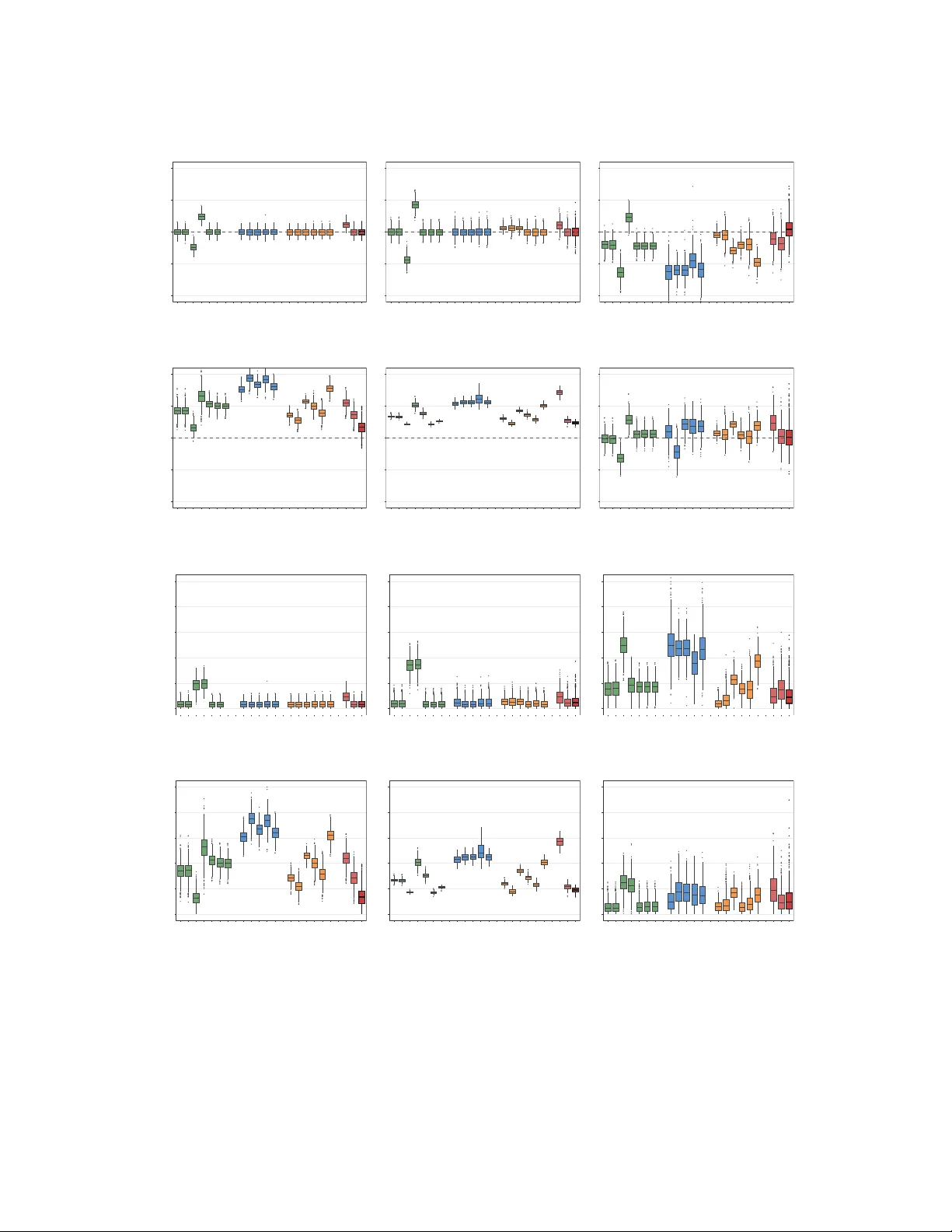
Join t Mo deling of Longitudinal EHR Data with Shared Random Eﬀects for Informativ e Visiting and Observ ation Pro cesses Cheng-Han Y ang 1 , Xu Shi 2 , and Bhramar Mukherjee ∗ 1 1 Departmen t of Biostatistics, Y ale Univ ersity 2 Departmen t of Biostatistics, Universit y of Michigan Abstract Longitudinal electronic health record data oﬀer unpreceden ted opportunities to study biomark er tra jectories in asso ciation with genetic, en vironmen tal, and social determinan ts of health. Ho wev er, asso ciation estimates from standard longitudinal models designed for regu- lar observ ation times ma y b e biased by a tw o-stage hierarchical missingness mechanism. The ﬁrst stage is the visiting proc ess, where encounters o ccur at irregular times largely driv en by patien t health status; it in tro duces a bias known as informativ e presence. The second stage is the observ ation pro cess: conditional on a visit occurring, biomarkers—the longitudinal outcomes of in terest—are selectively measured mostly based on clinical judgment and the underlying health tra jectory of the patient. This observ ation process induces a second source of bias termed informative observ ation. T wo critical gaps remain in this ﬁeld. First, the joint inﬂuence of these mec hanisms on statistical inference has not b een systematically ev aluated. Second, models accommodating both mec hanisms remain limited. T o address these gaps, we conduct extensiv e benchmarking studies and prop ose a uniﬁed semiparametric joint mo deling framew ork that sim ultaneously c haracterizes the visiting, biomark er observ ation, and longi- tudinal outcome processes. Cen tral to this framework is a shared sub ject-speciﬁc Gaussian laten t v ariable that captures unmeasured frailty and induces dep endence across all three comp onen ts. W e also introduce a sequential pro cedure that imputes missing biomarkers prior to adjusting for irregular visiting, and examine its p erformance. T o ensure computa- tional tractability for large-scale studies, we develop a three-stage estimation pro cedure and establish the consistency and asymptotic normalit y of our estimators. Sim ulation results demonstrate that our metho d yields un biased estimates under the t wo-stage hierarc hical mec hanism, whereas existing approac hes can b e substantially biased. In particular, metho ds that adjust only for irregular visiting ma y exhibit ev en greater bias than approac hes that ig- nore b oth mechanisms. W e further apply our framew ork—particularly suited for outpatient visiting settings—to data from the All of Us Researc h Program to in vestigate the asso ciation ∗ Corresp onding author: bhramar.mukherjee@y ale.edu 1 b et w een tw o neigh b orho od-level socio economic status indicators and the tra jectories of six biomark ers measured through blo od tests. Keyw ords: All of Us; Electronic health record; Informativ e observ ation pro cess; Informativ e visiting pro cess; Join t mo deling; Missing not at random. 1 In tro duction Longitudinal data collected in routine clinical care p ose inferential c hallenges that diﬀer funda- men tally from those in prosp ectiv e cohort studies or clinical trials. In designed studies, a protocol go verns b oth the sc hedule of patien t encoun ters and the panel of measuremen ts obtained at eac h encoun ter. In routine care, neither is predetermined; instead, b oth the timing of a visit and whether a particular biomark er is measured arise from a complex interpla y of disease severit y , clinical judgmen t, and patien t characteristics and b eha vior ( Hrip csak and Alb ers , 2013 ; Goldstein et al. , 2016 ). When these clinically driven mechanisms dep end on the latent health tra jectory under study , analyses that treat the data collection pro cess as ﬁxed or exogenous yield system- atically biased estimates of exp osure–biomark er asso ciations ( Lin et al. , 2004 ; Pullenay egum and Lim , 2016 ). These issues are of gro wing imp ortance as electronic health record (EHR) data are no w widely used in large-scale biomedical initiativ es suc h as the All of Us Researc h Program in the United States ( All of Us Researc h Program In vestigators , 2019 ) and the UK Biobank ( Bycroft et al. , 2018 ), where routinely collected lab oratory measuremen ts serv e as longitudinal outcomes for studying associations with clinical, demographic, genetic, en vironmen tal, b eha v- ioral, and so cial determinan ts of health. A prominent example is the laboratory-wide asso ciation study (LabW AS; Goldstein et al. , 2020 ; Dennis et al. , 2021 ), in which rep eated biomark er mea- suremen ts are link ed to genetic risk factors on a phenome-wide scale. Although LabW AS has yielded empirical insights, collapsing rep eated measurements into simple summaries neglects within-sub ject v ariability and fails to accoun t for the informative nature of the data collection pro cess. Sp eciﬁcally , tw o clinically driv en mechanisms—the timing of visits and the decision to measure a particular biomarker—distort the av ailable data in wa ys that standard metho ds do not address. These tw o mec hanisms reﬂect a t wo-stage hierarch y inherent in EHR data collection (Fig- ure 1 ). The ﬁrst stage is the visiting pro cess, which generates patien t encounters at irregular, clinically driven times. When patien ts with greater disease burden visit more frequen tly , the resulting o v errepresen tation of adv erse health states introduces a bias known as informativ e presence (IP; Lin et al. , 2004 ; Sun et al. , 2007 ). Ho wev er, the direction of bias under IP is not deﬁnitiv e: limited access to care may reduce visit frequency among the sic kest patients ( Ob ermey er et al. , 2019 ), while heterogeneities in diagnostic testing rates may inﬂate encoun ter frequency ( Ellen b ogen et al. , 2024 ), making the magnitude and sign of bias under IP diﬃcult to determine a priori . The second stage is the observ ation process: conditional on a visit o ccurring, a clinician decides whether to measure the biomark er of in terest—which serv es as the longi- 2 tudinal outcome in our mo deling framework—based on the patient’s current symptoms, prior test results, and clinical judgment. When this decision dep ends on factors related to the health tra jectory that are not fully captured by observ ed cov ariates, it giv es rise to a second source of bias that we term informativ e observ ation (IO; W ells et al. , 2013 ; Haneuse and Daniels , 2016 ). Consider patien t 2 in the left panel of Figure 1 as an illustration of this hierarch y . A t the ﬁrst visit, denoted by an op en circle, no lab oratory measuremen t is taken, reﬂecting the absence of clinical indication. At the second visit, a measuremen t is observed (solid dot) in resp onse to an adv erse condition. Finally , at the third visit, a follo w-up measurement is obtained to conﬁrm reco very; notably , this decision is conditional on b oth the patient’s curren t condition and clin- ical history . In the All of Us data, biomarker measuremen ts are observ ed only at a fraction of outpatien t visits; for example, even among patien ts with at least one glucose record, the median p er-patien t measurement rate is only 9.1%. The extent of missingness v aries substan tially across biomark ers (T able 4 ). Moreov er, this missingness is unlikely to b e ignorable: the unmeasured factors driving b oth the frequency of visits and the decision to measure—including laten t health status, access to care, and heterogeneit y in clinical decision-making—are often correlated with the biomark er tra jectory under study , so that b oth stages constitute a missing not at random (MNAR) mechanism that cannot be resolv ed by addressing either stage in isolation. Patien t 1 X V 1 X O 1 ( t ) X Y 1 ( t ) t 11 t 12 t 13 t 14 Y 1 ( t 11 ) NA Y 1 ( t 13 ) NA Patien t 2 X V 2 X O 2 ( t ) X Y 2 ( t ) t 21 t 22 t 23 NA Y 2 ( t 22 ) Y 2 ( t 23 ) Patien t 3 X V 3 X O 3 ( t ) X Y 3 ( t ) t 31 NA ID t X V X O ( t ) X Y ( t ) R Y i ( t ) Y i ( t ) 1 t 11 X V 1 X O 1 ( t 11 ) X Y 1 ( t 11 ) 1 Y 1 ( t 11 ) 1 t 12 X V 1 X O 1 ( t 12 ) X Y 1 ( t 12 ) 0 NA 1 t 13 X V 1 X O 1 ( t 13 ) X Y 1 ( t 13 ) 1 Y 1 ( t 13 ) 1 t 14 X V 1 X O 1 ( t 14 ) X Y 1 ( t 14 ) 0 NA 2 t 21 X V 2 X O 2 ( t 21 ) X Y 2 ( t 21 ) 0 NA 2 t 22 X V 2 X O 2 ( t 22 ) X Y 2 ( t 22 ) 1 Y 2 ( t 22 ) 2 t 23 X V 2 X O 2 ( t 23 ) X Y 2 ( t 23 ) 1 Y 2 ( t 23 ) 3 t 31 X V 3 X O 3 ( t 31 ) X Y 3 ( t 31 ) 0 NA . . . . . . . . . . . . . . . . . . . . . Figure 1: Illustration of the hierarchical data generation pro cess in volving Informative Presence (IP) and Informative Observ ation (IO). Left panel: Patien t timelines where clinic visits (ticks) are generated by the visiting pro cess driven b y cov ariates X V i . At each visit, the observ ation pro cess (driven by X O i ( t ) ) determines whether the biomarker outcome Y i ( t ) is measured (solid dots, R Y i ( t ) = 1 ) or unmeasured (hollow circles, R Y i ( t ) = 0 ), while the underlying longitudinal biomark er tra jectory is driven b y X Y i ( t ) . Right panel: The resulting long-format dataset used for analysis, where “NA” in the Y i ( t ) column indicates an unmeasured outcome ( R Y i ( t ) = 0 ) despite the patient’s presence at the clinic. The statistical literature on longitudinal EHR analysis (e.g., Gasparini et al. , 2020 ) has fo- cused predominan tly on the IP mechanism, the ﬁrst stage of the hierarc hy , when estimating outcome biomarker tra jectories. Such approac hes include in v erse intensit y w eigh ting ( Robins 3 et al. , 2000 ; Lin and Ying , 2001 ; Burvzko v a and Lumley , 2007 ; Yiu and Su , 2025 ), pairwise lik eliho o d ( Chen et al. , 2015 ; Shen et al. , 2019 ), and joint mo deling of the visiting and longitu- dinal pro cesses through shared frailties ( Liang et al. , 2009 ; Dai and Pan , 2018 ; W eav er et al. , 2023 ). While these approaches hav e substan tially adv anced the analysis of irregularly observ ed longitudinal data, they share a common limitation: each implicitly assumes that a clinic visit guaran tees measurement of the biomark er of interest—that is, they address IP while treating the observ ation stage as nonexistent. Although the Bay esian framework prop osed by Anthopolos et al. ( 2021 ) considers b oth IP and IO, the approach remains computationally in tractable for large-scale EHR data. A recent contribution, EHRJoint ( Du et al. , 2025 ), ac kno wledges the t wo-stage structure b y sp ecifying separate mo dels for the visiting, observ ation, and longitudinal outcome pro cesses. How ever, its observ ation mo del is form ulated as an indep enden t regression on observ ed cov ariates. This formulation fails to capture unmeasured heterogeneit y—such as pa- tien t health a w areness, access to care, or unrecorded clinical intuition—that join tly determines the timing of encounters, the necessity of testing, and the biomarker tra jectories. This restriction is equiv alen t to treating the observ ation mechanism as missing at random (MAR) conditional on observ ed co v ariates, limiting its ability to accommo date the MNAR mechanism iden tiﬁed ab o v e. T o address these challenges, w e make tw o main contributions. First, w e prop ose GIVEHR (Gaussian Informative Visiting and observ ation pro cesses in Electronic Health Records), a semi- parametric joint mo deling framework. P articularly well-suited to outpatien t settings, it explic- itly accommo dates the tw o-stage hierarch y of EHR data collection. Unlike existing metho ds, GIVEHR links visit in tensity , observ ation mechanisms, and biomarker tra jectories through a shared Gaussian latent v ariable. This structure captures unmeasured heterogeneit y while yield- ing closed-form marginal likelihoo ds, enabling a computationally eﬃcien t estimation pro cedure that scales to large EHR databases. In contrast to the Ba yesian framew ork of Anthopolos et al. ( 2021 ), which requires time discretization, GIVEHR operates in con tin uous time, preserving the irregular visit structure characteristic of EHR data. In eﬀect, GIVEHR enables v alid infer- ence b y accommo dating the MNAR mec hanisms inherent in b oth the visiting and observ ation pro cesses—a c hallenge that existing methods leav e unresolved. W e establish the consistency and asymptotic normalit y of the prop osed estimators under regularity conditions. Second, we provide the ﬁrst systematic ev aluation of 20 existing approaches under joint IP and IO mechanisms. These approaches can b e broadly categorized into four classes: outcome- only metho ds, whic h ignore b oth IP and IO; IP-only adjustmen ts, whic h correct for irregular visiting but assume the biomarker is measured at ev ery visit; imputation-based pip elines, which impute missing biomarkers b efore applying an IP correction; and joint IP+IO framew orks, which mo del both stages sim ultaneously . Since no prior work has combined imputation with IP correc- tion as describ ed ab o v e, w e introduce and ev aluate this pip eline against the other approac hes. A k ey ﬁnding of this ev aluation is that partial corrections can b e coun terpro ductiv e: adjusting for IP while ignoring IO can amplify bias relative to naïve analyses that ignore b oth stages en- tirely , b ecause IP-only metho ds implicitly assume that every clinic visit yields a measurement, 4 forcing the model to misattribute unmo deled observ ation bias to the visiting pro cess itself— thereb y amplifying, rather than removing, the underlying distortion. Simulatio ns demonstrate that, when the joint MNAR mechanism is correctly sp eciﬁed, GIVEHR yields appro ximately un biased estimates, whereas existing metho ds exhibit substantial bias. Under departures from this sp eciﬁcation, GIVEHR still considerably reduces bias relative to all comp eting approac hes. W e further apply GIVEHR to the All of Us Researc h Program to inv estigate the asso ciation b e- t ween tw o neigh b orho od-level so cioeconomic status indicators and longitudinal tra jectories of six clinical biomark ers. Because the visiting pro cess is shared across biomarkers for a giv en patien t, this design allows us to con trast v arying observ ation mec hanisms—ranging from routine to highly targeted tests—under a common IP structure. This application demonstrates the scalabilit y of GIVEHR to large-scale EHR data and illustrates how accounting for the MNAR mec hanisms in b oth the visiting and observ ation pro cesses can substantially change the magnitude of estimated so cioeconomic–biomarker associations. The remainder of this pap er is organized as follows: Sections 2 and 3 detail the GIVEHR mo del sp eciﬁcation and estimation pro cedure, resp ectiv ely; Section 4 establishes the asymptotic theory; Section 5 reviews existing metho ds; Section 6 presents the sim ulation study; Section 7 describ es the application to the All of Us data; and Section 8 concludes with a discussion. 2 Metho d 2.1 Mo del Sp eciﬁcation In a study comprising n patients, let m i denote the total n umber of visits for sub ject i , and let Y i ( t ) represen t the longitudinal biomark er pro cess observ ed o ver the windo w t ∈ [0 , τ ] . The follo w-up time for each patient is restricted to this interv al and is further limited by a random censoring time C i . The collection of biomark er measurements in the EHR system can b e char- acterized by three pro cesses: the visiting pro cess, the observ ation pro cess, and the longitudinal pro cess. T o account for the MNAR mec hanisms that arise when all three pro cesses are driv en by unmeasured clinical heterogeneit y , we p osit a shared, sub ject-level latent v ariable U i ∼ N (0 , 1) that captures unmeasured patient tendencies and induces dependence among all three processes. The Gaussian sp eciﬁcation places the laten t v ariable on the same scale as the random comp o- nen ts in all three submodels, yielding transparen t cross-pro cess dep endence, closed-form marginal lik eliho o ds, and a scalable estimation pro cedure, as w e detail below. Eac h pro cess may dep end on distinct but p ossibly o verlapping observ ed cov ariate sets. Let X V i denote baseline cov ariates for the visiting pro cess, X O i ( t ) time-v arying cov ariates for the observ ation pro cess, and X Y i ( t ) co v ariates for the longitudinal outcome. In the observ ation and outcome mo dels, sub vectors Z O i ( t ) ⊆ X O i ( t ) and Z Y i ( t ) ⊆ X Y i ( t ) are asso ciated with sub ject- sp eciﬁc random co eﬃcien ts linked to U i . The visiting pro cess dep ends solely on a scalar frailty , as visit in tensit y is primarily driven b y aggregate health burden rather than co v ariate-sp eciﬁc 5 random eﬀects. The visiting pro cess captures the temp oral pattern of patients’ clinical visits. Let N i ( t ) b e the visit counting pro cess with jumps d N i ( t ) ∈ { 0 , 1 } at visit times. Conditional on U i and X V i , w e assume a m ultiplicative in tensity mo del for the visiting pro cess: E  d N i ( t ) | U i , X V i  = I ( t ≤ C i ) η i exp( γ ⊤ X V i )dΛ 0 ( t ) (1) where dΛ 0 ( t ) = λ 0 ( t ) d t is an unspeciﬁed baseline in tensity function, γ denotes the v ector of regression coeﬃcients, and I ( t ≤ C i ) is an indicator function, taking the v alue 1 if the patient is at risk at time t , and 0 otherwise. The term η i represen ts a sub ject-sp eciﬁc multiplicativ e frailt y that accoun ts for unmeasured heterogeneit y in visit in tensity . Unlike Liang et al. ( 2009 ) and Du et al. ( 2025 ), who adopt a gamma frailty for its conjugacy with the P oisson-type visit lik eliho od, w e specify η i = exp( µ 0 + σ U i ) as lognormal. The lognormal sp eciﬁcation ensures that the full v ector of laten t v ariables is join tly Gaussian, preserving closed-form conditional distributions throughout the estimation procedure. A gamma frailt y w ould break this joint normalit y , requiring numerical integration ov er the full random eﬀects v ector whose dimension grows with the n umber of random co eﬃcien ts in the observ ation and outcome pro cesses. W e constrain µ 0 = − σ 2 / 2 so that E( η i ) = 1 , ensuring iden tiﬁability ( Co ok et al. , 2007 ). A dditionally , the observ ation pro cess determines whether the biomark er of interest, Y i ( t ) , is observ ed at a giv en visit time t . Let R Y i ( t ) ∈ { 0 , 1 } b e the observ ation indicator, conditional on a visit o ccurring (i.e., d N i ( t ) = 1 ). W e form ulate the probability of observ ation using a probit mixed eﬀects mo del, as the normal cum ulative distribution function (CDF) comp osed with normally distributed random eﬀects admits a closed-form marginal probability—a prop ert y not shared by the logit link—thereby maintaining the analytical tractabilit y of the Gaussian laten t structure: pr  R Y i ( t ) = 1 | d N i ( t ) = 1 , U i , X O i ( t ) , Z O i ( t )  = Φ n α ⊤ X O i ( t ) + q ⊤ i Z O i ( t ) o (2) where Φ( · ) denotes the standard normal CDF. The v ector q i represen ts sub ject-speciﬁc random co eﬃcien ts that capture unmeasured factors driving the observ ation decision b ey ond what is explained b y observ ed co v ariates. T o capture the dep endency on the shared latent structure, w e assume q i | U i ∼ N ( δ U i , Σ q ) where δ go verns the dep endence betw een the shared laten t v ariable and the propensity to observ e. 6 When δ  = 0 , the observ ation pro cess dep ends on the latent v ariable that also driv es the biomark er tra jectory , inducing the MNAR mechanism discussed ab o ve; setting δ = 0 reduces the observ a- tion mo del to MAR. F or brevit y , we deﬁne ω i ( t ; α , δ , Σ q , U i ) = pr  R Y i ( t ) = 1 | d N i ( t ) = 1 , U i , X O i ( t ) , Z O i ( t )  . The longitudinal pro cess characterizes the biomarker tra jectory ov er time. The biomarker v alue, Y i ( t ) , is observ ed only when a visit occurs and the biomark er is measured (i.e., d N i ( t ) = 1 and R Y i ( t ) = 1 ). W e assume a semiparametric mo del with random eﬀects for the tra jectory: Y i ( t ) = β 0 ( t ) + β ⊤ X Y i ( t ) + b ⊤ i Z Y i ( t ) + ε i ( t ) (3) where β denotes the ﬁxed-eﬀect co eﬃcien ts corresp onding to X Y i ( t ) and ε i ( t ) ∼ N (0 , σ 2 ε ) repre- sen ts the random error. The baseline mean function β 0 ( t ) is left unsp eciﬁed, a voiding the need to select a parametric form for the temporal trend and providing robustness against missp eciﬁcation of the time eﬀect. The random eﬀects b i are linked to the shared factor U i via b i | U i ∼ N ( θ U i , Σ b ) , where θ pla ys an analogous role to δ in the observ ation pro cess: it go verns ho w the shared latent v ariable shifts the biomarker tra jectory . F or instance, when σ > 0 and θ > 0 , patien ts who visit more frequently also tend to ha ve higher biomark er v alues, capturing the p ositiv e confounding structure commonly encountered in clinical data. On the other hand, setting θ = 0 remo ves the dep endence b et ween the longitudinal pro cess and the latent v ariable, reducing the outcome mo del to a standard linear mixed mo del. The shared laten t v ariable U i induces a coheren t dep endence structure across the three sub- mo dels. Deﬁne ζ i = µ 0 + σ U i and rewrite b i = θ U i + e b i and q i = δ U i + e q i , where ( e b i , e q i ) are indep enden t of U i . Then ( ζ i , b ⊤ i , q ⊤ i ) ⊤ is multiv ariate normal with co v ariance matrix v ar    ζ i b i q i    =     σ 2 σ θ ⊤ σ δ ⊤ σ θ θ θ ⊤ + Σ b θ δ ⊤ σ δ δ θ ⊤ δ δ ⊤ + Σ q     . The oﬀ-diagonal blo c ks rev eal the cross-pro cess dep endence implied by the model. F or example, σ θ ⊤ quan tiﬁes the co v ariance b et ween visit intensit y and the biomarker tra jectory , while θ δ ⊤ captures the association b et ween the biomark er tra jectory and the prop ensit y to b e observed. This explicit, interpretable dep endence structure is the central adv an tage of the Gaussian laten t sp eciﬁcation—it is precisely this structure that allows GIVEHR to correct for the join t MNAR mec hanism induced b y IP and IO. The parameters to b e estimated are organized according to the three submo dels. F or the visiting pro cess, these include the regression coeﬃcients γ , the frailty parameter σ , and the non-parametric baseline intensit y Λ 0 ( t ) . The observ ation pro cess in volv es the ﬁxed eﬀects α , the dep endence vector δ , and the co v ariance matrix Σ q . Finally , the longitudinal pro cess en- 7 compasses the ﬁxed eﬀects β , the dep endence vector θ , and the cov ariance matrix Σ b . The comprehensiv e estimation pro cedure for these components is detailed in Section 3 . 2.2 Assumptions These assumptions serve distinct functions within the GIVEHR framew ork, bridging theoretical rigor with computational eﬃciency . Assumptions 2.1 and 2.2 establish the indep endence struc- tures necessary for un biased parameter estimation, while Assumption 2.3 speciﬁes the parametric forms that enable closed-form represen tations of the empirical Ba yes p osterior and marginalized observ ation probabilities. Assumption 2.1 (Noninformativ e censoring) . The c ensoring time C i is assume d to b e noninfor- mative. Sp e ciﬁc al ly, c onditional on the c ovariates { X V i , X O i ( t ) , X Y i ( t ) } , C i is indep endent of the visiting pr o c ess N i ( · ) , the observation pr o c ess R Y i ( · ) , and the longitudinal outc ome Y i ( · ) . This assumption ensur es that the c ensoring me chanism do es not intr o duc e additional bias in mo del estimation. Assumption 2.2 (Conditional indep endence of data collection and outcome errors) . Given the shar e d latent variable U i and al l observe d c ovariates, the visiting, observation, and longitudinal outc ome pr o c esses ar e c onditional ly indep endent:  N i ( t ) , R Y i ( t )  ⊥ { ε i ( t ) }    U i , X V i , X O i ( t ) , X Y i ( t )  . This c ondition p ermits the factorization of the joint likeliho o d, justifying the sep ar ability of the estimation pr o c e dur e. Assumption 2.3 (latent v ariable and random-eﬀect distributions) . Conditional on U i , the r an- dom slop es in the observation submo del fol low a multivariate normal distribution, q i | U i ∼ N ( δ U i , Σ q ) . In the longitudinal submo del, the r andom eﬀe cts satisfy the c onditional me an link b i | U i ∼ N ( θ U i , Σ b ) . This Gaussian sp e ciﬁc ation, c ombine d with the pr obit link in ( 2 ) , enables a close d-form mar ginal- ization of the latent variable and avoids the ne e d for high-dimensional numeric al inte gr ation. 8 Visiting Process Observ ation Proce ss Outcome Process Stage 1 Stage 2 Stage 3 γ , Λ 0 ( t ) , σ 2 α , δ , Σ q β , θ Empirical Ba y es Posterior: µ U i , s 2 U i Marginal Probabilit y: ω i ( t ) Stage P arameter Description 1 (Visiting) γ Co v ariate eﬀects on visit intensit y Λ 0 ( t ) Baseline cum ulativ e intensit y σ 2 F railty v ariance ( µ U i , s 2 U i ) Empirical Ba yes p osterior of laten t v ariable U i | ( C i , m i ) 2 (Observ ation) α Fixed eﬀects on observ ation probability δ Eﬀect of latent U i on observ ation Σ q Random slop e cov ariance ω i ( t ) Marginalized observ ation probability 3 (Outcome) β Co v ariate eﬀects on biomarker Y θ Eﬀect of laten t U i on Y Figure 2: Three-stage estimation procedure. Gra y shaded b o xes indicate laten t information transmitted across stages. Stages 1 and 2 estimate nuisance parameters to estimate the empirical Ba yes p osterior and marginalized observ ation probabilities, respectively; these quantities are subsequen tly incorporated in to Stage 3 to correct for clinically informed bias. 3 Three-Stage Estimation 3.1 Ov erview W e prop ose a three-stage estimation pro cedure summarized in Figure 2 . In the ﬁrst stage, w e estimate nuisance parameters gov erning the visiting pro cess and deriv e an empirical Bay es p osterior for the latent v ariable U i . In the second stage, we estimate the observ ation pro cess parameters and obtain the marginalized observ ation probabilit y ω i ( t ) . In the third stage, these quan tities are used to construct a comp ensation co v ariate that corrects for bias in the weigh ted least squares (WLS) estimation of the target longitudinal outcome parameters ( β , θ ) . 9 3.2 Stage 1: Visiting Pro cess W e estimate γ by maximizing the partial lik eliho o d for the m ultiplicative intensit y mo del ( 1 ). The corresp onding score equation tak es the form n X i =1 Z τ 0 n X V i − X V ( t ) o d N i ( t ) = 0 , (4) where X V ( t ) = P n j =1 I ( t ≤ C j ) exp  γ ⊤ X V j  X V j  P n j =1 I ( t ≤ C j ) exp  γ ⊤ X V j  is the risk-set a verage at time t . This is the Andersen–Gill extension ( Andersen and Gill , 1982 ) of the Co x partial likelihoo d score equation to recurren t even ts, treating each visit as a recurrent ev ent within a counting pro cess framew ork. Given b γ , the baseline cumulativ e intensit y is estimated via the Breslow estimator ( Breslo w , 1974 ): b Λ 0 ( t ) = n X i =1 Z t 0 d N i ( s ) P n j =1 I ( s ≤ C j ) exp( b γ ⊤ X V j ) . (5) Deﬁne the estimated exp ected cum ulative in tensity b y b ν i := exp  b γ ⊤ X V i  b Λ 0 ( C i ) . Let σ 2 η := v ar( η i ) denote the common frailt y v ariance. This v ariance is estimated using the metho d of momen ts based on the observ ed visit coun ts m i for patient i : b σ 2 η = max ( 0 , P n i =1  m 2 i − m i − b ν 2 i  P n i =1 b ν 2 i ) . (6) Assuming log η i ∼ N ( µ 0 , σ 2 ) sub ject to E( η i ) = 1 , we obtain b σ 2 = log { 1 + c v ar( η i ) } and b µ 0 = − b σ 2 / 2 . Subsequen tly , w e approximate the empirical Ba yes p osterior b y a normal distribution via a Laplace approximation ( Tierney and Kadane , 1986 ) (Lemma S1 ), U i | ( C i , m i ) ≈ N ( µ U i , s 2 U i ) , where µ U i is the p osterior mo de and s 2 U i is the negative inv erse Hessian of the log-p osterior of U i ev aluated at µ U i . Lemma S1 further demonstrates that the p osterior is strictly log-concav e in U i , which guaran tees a unique p osterior mo de µ U i and a uniquely determined s 2 U i . 3.3 Stage 2: Observ ation Pro cess T o construct the lik eliho o d for the observ ation indicators R Y i ( t ) , we require the observ ation probabilit y a veraged ov er uncertaint y in U i . Using the empirical Bay es p osterior from Stage 1, 10 w e deﬁne the marginalized observ ation probabilit y ω i ( t ) := E { ω i ( t ; U i ) | C i , m i } . By probit–normal conjugacy (Lemma S3 ), this admits a closed-form representation: ω i ( t ) = Φ { k i ( t ) } , where k i ( t ) := α ⊤ X O i ( t ) +  δ ⊤ Z O i ( t )  µ U i q 1 +  Z O i ( t )  ⊤ Σ q Z O i ( t ) +  δ ⊤ Z O i ( t )  2 s 2 U i . With the marginalized observ ation probabilit y ω i ( t ) deﬁned for each visit, the parameters ( α , δ , Σ q ) are estimated b y maximizing the comp osite Bernoulli log-likelihoo d function, summed ov er all visit times in [0 , τ ] for all sub jects: ℓ IO ( α , δ , Σ q ) = n X i =1 Z τ 0 h R Y i ( t ) log  ω i ( t )  +  1 − R Y i ( t )  log  1 − ω i ( t )  i d N i ( t ) . (7) The resulting estimators ( b α , b δ , b Σ q ) are the v alues that maximize this function, sub ject to b Σ q b eing p ositiv e semi-deﬁnite. F or notational brevity , we denote the plug-in estimate as b ω i ( t ) := ω i  t ; b α , b δ , b Σ q  . 3.4 Stage 3: Longitudinal Outcome Mo del Conditional on the follow-up time C i and the n umber of visits m i , estimation of the outcome parameters relies on a mean-zero pro cess M i ( t ) . F ollowing Liang et al. ( 2009 ), the conditional exp ectation of the outcome incremen t is corrected for IP and IO mechanisms driv en b y U i . W e deﬁne the observ ation-weigh ted p osterior mean ratio as κ i ( t ) := E { U i ω i ( t ; U i ) | C i , m i } ω i ( t ) = µ U i +  δ ⊤ Z O i ( t )  s 2 U i q 1 +  Z O i ( t )  ⊤ Σ q Z O i ( t ) +  δ ⊤ Z O i ( t )  2 s 2 U i ϕ { k i ( t ) } Φ { k i ( t ) } , where ϕ ( · ) denotes the probability densit y function of the standard normal distribution. As demonstrated in Lemma S3 , κ i ( t ) admits a closed-form represen tation, which simpliﬁes the sub- sequen t computation of the marginal lik eliho o d. A compensation co v ariate is then constructed as B i ( t ) := Z Y i ( t ) κ i ( t ) . Deﬁne the weigh t function for sub ject i at time t as p i ( t ) = ω i ( t ) I ( t ≤ C i ) m i Λ 0 ( C i ) , (8) 11 whic h corrects for t wo distinct sources of clinically informative sampling. The marginalized observ ation probability ω i ( t ) adjusts for the informative observ ation pro cess, whereas the factor I ( t ≤ C i ) m i / Λ 0 ( C i ) adjusts for the informative visiting pro cess. This latter term arises from Lemma S1 , which establishes that, conditional on the follow-up window C i and the total num b er of visits m i , each visit is equally lik ely to o ccur at any p oin t along the baseline in tensity scale, i.e., E { d N i ( t ) | C i , m i } = I ( t ≤ C i ) m i dΛ 0 ( t ) / Λ 0 ( C i ) . The estimating equations for the cum ulative baseline function A ( t ) = R t 0 β 0 ( s ) dΛ 0 ( s ) and the regression parameters ( β , θ ) are deriv ed from the comp ensated process: M i ( t ) = Z t 0  Y i ( s ) − β ⊤ X Y i ( s ) − θ ⊤ B i ( s )  R Y i ( s ) d N i ( s ) − Z t 0 p i ( s ) d A ( s ) . (9) By Lemma S1 and the martingale comp ensation result in Lemma S2 , M i ( t ) is a zero-mean martingale at the true parameter v alues. W e solve these equations using a proﬁling approach. Summing the martingale represen tation o ver sub jects yields a Breslow-t yp e estimator for the baseline increment: d b A ( t ) = P n i =1  Y i ( t ) − β ⊤ X Y i ( t ) − θ ⊤ b B i ( t )  R Y i ( t ) d N i ( t ) P n i =1 b p i ( t ) , where b p i ( t ) is the plug-in estimate of ( 8 ). Substituting this back into the martingale represen ta- tion and rearranging yields a risk-set cen tered estimating equation for ( β , θ ) : n X i =1 Z τ 0 X Y i ( t ) − X Y ( t ) b B i ( t ) − b B ( t ) !  Y i ( t ) − β ⊤ X Y i ( t ) − θ ⊤ b B i ( t )  R Y i ( t ) d N i ( t ) = 0 , (10) where the centering terms are w eighted a verages o ver all sub jects at each time t : X Y ( t ) = P n i =1 X Y i ( t ) b p i ( t ) P n i =1 b p i ( t ) , b B ( t ) = P n i =1 b B i ( t ) b p i ( t ) P n i =1 b p i ( t ) . Solving this equation yields the estimators ( b β , b θ ) . The complete three-stage pro cedure is summarized in Algorithm 1 . Remark 3.1. The pr op ose d fr amework c an further ac c ommo date dep endenc e on the subje ct’s own observation p ast history. F or example, an abnormal biomarker value may pr ompt r ep e at testing. However, including history R Y i ( t − ) in the observation mo del intr o duc es endo geneity, sinc e p ast observation indic ators involve the same p atient-sp e ciﬁc latent variable that drives curr ent observation. Mor e over, c onditioning on the prior history br e aks the c onditional indep endenc e acr oss observation history, substantial ly incr e asing c omputational c ost. A mo diﬁe d estimation algorithm and additional simulation addr essing this issue ar e pr ovide d in Se ctions S7 and S8 of the Supplementary Material, r esp e ctively. 12 Algorithm 1 Three-stage estimation pro cedure for GIVEHR. 1: Step 1. Visiting pro cess estimation. 2: (a) Estimate ( γ , Λ 0 ( t ) , σ 2 ) using ( 4 )–( 6 ). 3: (b) Compute the empirical Bay es p osterior ( b µ U i , b s 2 U i ) via Laplace approximation (Lemma S1 ). 4: Step 2. Observ ation pro cess estimation. 5: Estimate ( α , δ , Σ q ) by maximizing ( 7 ), treating ( b µ U i , b s 2 U i ) from Step 1 as kno wn. 6: Step 3. Outcome pro cess estimation. 7: (a) Construct the comp ensation co v ariate b B i ( t ) = Z Y i ( t ) b κ i ( t ) and w eigh ts b p i ( t ) using estimates from Steps 1–2. 8: (b) Obtain ( b β , b θ ) from the closed-form w eigh ted least squares solution ( 10 ). 4 Asymptotic Prop erties of ( b β , b θ ) W e establish the large-sample b eha vior of the joint estimator ( b β , b θ ) , deﬁned as the solution to ( 10 ). Theorem 4.1 (Consistency) . Under Assumptions 2.1 – 2.3 and r e gularity c onditions (C1) – (C6) , let ( b β , b θ ) b e the solution to the estimating e quations ( 10 ) , wher e the c onditional exp e ctations involving U i ar e evaluate d using the L aplac e appr oximation. Then, as n → ∞ , b β b θ ! p − → β 0 θ 0 ! . Consistency holds pro vided that the appro ximation error in tro duced b y the Laplace metho d is asymptotically negligible under standard regularit y conditions. The pro of is detailed in Sup- plemen tary Section S6.3 . The asymptotic distribution of the estimator follo ws from standard martingale central limit theory , extending the results of Liang et al. ( 2009 ) and Du et al. ( 2025 ). Theorem 4.2 (Asymptotic normalit y) . Under Assumptions 2.1 – 2.3 and r e gularity c onditions (C1) – (C6) , if σ 2 > 0 , then as n → ∞ , √ n ( b β b θ ! − β 0 θ 0 !) d − → N  0 , W − 1 Γ  W − 1  , wher e the matric es W and Γ ar e deﬁne d in Supplementary Se ction S6.4 . The asymptotic v ariance W − 1 Γ W − 1 can be estimated via the plug-in method using the inﬂuence function decomp osition detailed in Section S6.4 of the Supplemen tary Material. The nonparametric b o otstrap oﬀers an alternative that av oids analytic deriv ations ( Liang et al. , 2009 ; 13 Du et al. , 2025 ), though at the cost of additional computational burden from repeated estimation across resampled datasets. 5 Existing Metho ds W e classify existing approaches for analyzing longitudinal EHR data into four broad categories based on the assumptions they make regarding the data generation mechanisms: (i) outcome- only methods that ignore the IP and IO mechanisms; (ii) IP-only methods that expli citly model the visiting process but assume complete observ ation at visits; (iii) imputation+IP metho ds that ﬁrst impute missing outcomes conditional on the visiting pro cess and then apply an IP-only mo del; and (iv) IP- and IO-aw are metho ds (IP+IO) that address b oth informative visiting and observ ation. T able 1 pro vides a summary of these approaches. 5.1 Outcome-Only Metho ds The simplest method, frequen tly emplo yed in high-throughput phenot yping studies, inv olves re- ducing the longitudinal tra jectory to a single cross-sectional summary statistic, such as the mean, median, or maxim um of the observ ed measurements. This derived outcome is then regressed on co v ariates. While computationally con venien t, this approac h discards temporal information and yields biased estimates when the frequency of measuremen t is correlated with disease severit y . The other standard statistical framework for analyzing such longitudinal data is the linear mixed-eﬀects mo del (LMM). This approac h models the outcome tra jectory Y i ( t ) as: Y i ( t ) = β 0 ( t ) + β ⊤ X Y i ( t ) + b ⊤ i Z Y i ( t ) + ε i ( t ) , where β 0 ( t ) is a baseline mean function, b i ∼ N ( 0 , Σ b ) are sub ject-sp eciﬁc random eﬀects, and ε i ( t ) ∼ N (0 , σ 2 ε ) . Estimation is typically performed via restricted maximum lik eliho od (REML) conditional on the realized observ ation times. T o mitigate clinically informed bias within the LMM framew ork without fully mo deling the visiting process, augmented sp eciﬁcations in tro duce constructed v ariables to serv e as pro xies for the unobserv ed health status. The Visit-A ware LMM (V A-LMM) assumes that the cum ulative n umber of visits up to time t , denoted H N i ( t ) = R t 0 d N i ( s ) , acts as a surrogate for disease sev erity (or frailty) and includes it as an additional time-v arying cov ariate ( Goldstein et al. , 2016 ): Y i ( t ) = β 0 ( t ) + β ⊤ X Y i ( t ) + γ N H N i ( t ) + b ⊤ i Z Y i ( t ) + ε i ( t ) . Similarly , the Observ ation-A ware LMM (O A-LMM) emplo ys the historical coun t of actual biomark er measuremen ts, H R i ( t ) = R t 0 R Y i ( s )d N i ( s ) , as a proxy to capture the IP and IO mechanism. 14 5.2 IP-Only Metho ds Metho ds in this class explicitly account for the visiting pro cess N i ( t ) to correct for IP , but generally assume that the observ ation pro cess is noninformativ e, implying that if a patient visits, the biomarker is observ ed with probability one (i.e., R Y i ( t ) ≡ 1 ). One widely used approach in volv es Inv erse Intensit y Rate Ratio (I IRR-W eighting) ( Lin and Ying , 2001 ; Burvzko v a and Lumley , 2007 ). These methods adopt a marginal mo deling persp ec- tiv e, specifying a proportional rates mo del for the visiting pro cess, λ i ( t ) = λ 0 ( t ) exp  γ ⊤ X V i ( t )  , and estimating regression parameters β b y solving a w eighted estimating equation: n X i =1 Z τ 0 1 b V i ( t ) D i ( t ) n Y i ( t ) − β ⊤ X Y i ( t ) o d N i ( t ) = 0 , where b V i ( t ) is the estimated relativ e visit intensit y . W e refer to this approac h as IIRR weigh ting. The v alidity of IIRR hinges on the Visiting-at-Random (V AR) assumption: d N i ( t ) ⊥ Y i ( t ) | H i ( t − ) , where H i represen ts observ ed history . Extensions using balancing weigh ts ( Yiu and Su , 2025 ) hav e b een prop osed to robustify estimation against misspeciﬁcation of the visiting intensit y λ i ( t ) ; we refer to this approac h as IIRR-Balanced. Alternativ ely , pairwise comp osite lik eliho o d metho ds ( Chen et al. , 2015 ; Shen et al. , 2019 ), denoted as P airLik, a void full sp eciﬁcation of the visiting pro cess by constructing an ob jective function based on pairs of observ ations conditioned on their order. Under the assumption that the visiting pro cess satisﬁes a separabilit y condition (factorizing in to outcome-dependent and co v ariate-dep enden t components), n uisance parameters gov erning the visiting process cancel out. The estimator for β is obtained b y maximizing the pairwise ob jective function: ℓ p ( β ) = X i 0 , deﬁne Y = a + bX + dU . Then Y ∼ N ( a + bµ X , b 2 σ 2 X + d 2 ) . L et k = a + bµ X q b 2 σ 2 X + d 2 . Then E  Φ  a + bX d  = Φ( k ) , (S2) E  X Φ  a + bX d  = µ X Φ( k ) + bσ 2 X q b 2 σ 2 X + d 2 ϕ ( k ) , (S3) E  X Φ  a + bX d  E  Φ  a + bX d  = µ X + bσ 2 X q b 2 σ 2 X + d 2 ϕ ( k ) Φ( k ) . (S4) Pr o of. Note that Φ(( a + bX ) /d ) = pr { U ≤ ( a + bX ) /d | X } . By the la w of total exp ectation, E  Φ  a + bX d  = E  pr  U ≤ a + bX d     X  = pr( dU ≤ a + bX ) = pr( Y ≥ 0) . Since Y is normal with mean a + bµ X and v ariance b 2 σ 2 X + d 2 , standardization yields pr( Y ≥ 0) = pr( Z ≥ − k ) = Φ( k ) for Z ∼ N (0 , 1) , proving ( S2 ). F or ( S3 ), write E { X Φ(( a + bX ) /d ) } = E { X 1 { Y ≥ 0 }} . Because ( X , Y ) is jointly normal, w e can express X in terms of the standardized v ariable Z = ( Y − E( Y )) / p v ar( Y ) : E( X | Z = z ) = µ X + cov( X , Z ) z . Computing the cov ariance: Z = b ( X − µ X ) + dU q b 2 σ 2 X + d 2 , so co v ( X, Z ) = bσ 2 X q b 2 σ 2 X + d 2 . No w in tegrate ov er z in the region where Y ≥ 0 , i.e., Z ≥ − k : E { X 1 { Y ≥ 0 }} = Z ∞ − k E( X | Z = z ) ϕ ( z ) dz = Z ∞ − k   µ X + bσ 2 X q b 2 σ 2 X + d 2 z   ϕ ( z ) dz = µ X Z ∞ − k ϕ ( z ) dz + bσ 2 X q b 2 σ 2 X + d 2 Z ∞ − k z ϕ ( z ) dz . S4 Using R ∞ − k ϕ ( z ) dz = Φ( k ) and R ∞ − k z ϕ ( z ) dz = ϕ ( k ) , we obtain ( S3 ). Dividing ( S3 ) b y ( S2 ) yields ( S4 ). Corollary S2.1 (Closed-form approximation for κ i ( t ) ) . Under the mo del sp e ciﬁc ation, the observation- weighte d p osterior me an r atio κ i ( t ) has the close d form: κ i ( t ) = E { U i ω i ( t ; U i ) | C i , m i } E { ω i ( t ; U i ) | C i , m i } = µ U i + ( δ ⊤ Z O i ) s 2 U i q 1 + ( Z O i ) ⊤ Σ q Z O i + ( δ ⊤ Z O i ) 2 s 2 U i ϕ { k i ( t ) } Φ { k i ( t ) } , wher e ( µ U i , s 2 U i ) ar e the EB p osterior me an and varianc e of U i | ( C i , m i ) , and k i ( t ) = α ⊤ X O i + ( δ ⊤ Z O i ) µ U i q 1 + ( Z O i ) ⊤ Σ q Z O i + ( δ ⊤ Z O i ) 2 s 2 U i . Pr o of. Apply Lemma S3 with X = U i | ( C i , m i ) ∼ N ( µ U i , s 2 U i ) , a = α ⊤ X O i , b = δ ⊤ Z O i , and d = q 1 + ( Z O i ) ⊤ Σ q Z O i . Then ( S4 ) giv es the stated formu la. S3 Mean-Zero Prop ert y of the Comp ensated Pro cess This section establishes that the comp ensated pro cess M i ( t ) deﬁned in the man uscript satisﬁes E { M i ( t ) | C i , m i } = 0 at the true parameter v alues. This is the foundational result enabling consisten t estimation. Prop osition S3.1 (Conditional mean-zero prop ert y) . Under the mo del sp e ciﬁc ation in Se c- tion S6.1 , deﬁne the c omp ensate d pr o c ess M i ( t ) = Z t 0  Y i ( s ) − β ⊤ 0 X Y i ( s ) − θ ⊤ 0 B i, 0 ( s )  R Y i ( s ) d N i ( s ) − Z t 0 p i, 0 ( s ) d A 0 ( s ) , (S5) wher e B i, 0 ( s ) = κ i, 0 ( s ) Z Y i ( s ) , p i, 0 ( s ) = ω i, 0 ( s ) 1 ( s ≤ C i ) m i / Λ 0 ( C i ) , and the subscript “ 0 ” denotes evaluation at the true p ar ameter values. Then E  M i ( t ) | C i , m i  = 0 for al l t ∈ [0 , τ ] . Pr o of. The pro of proceeds by decomposing the outcome residual and computing each term’s conditional exp ectation separately . Step 1: Decomp osition of the outcome residual. Under the true mo del: Y i ( s ) = β 0 ( s ) + β ⊤ 0 X Y i ( s ) + b ⊤ i Z Y i ( s ) + ε i ( s ) , S5 where b i = θ 0 U i + e b i , and e b i ∼ N ( 0 , Σ b ) is the residual outcome random eﬀect. Substituting in to the residual: Y i ( s ) − β ⊤ 0 X Y i ( s ) − θ ⊤ 0 B i, 0 ( s ) = β 0 ( s ) + θ ⊤ 0 U i Z Y i ( s ) + e b ⊤ i Z Y i ( s ) + ε i ( s ) − θ ⊤ 0 κ i, 0 ( s ) Z Y i ( s ) = β 0 ( s ) | {z } (I) + θ ⊤ 0 { U i − κ i, 0 ( s ) } Z Y i ( s ) | {z } (II) + e b ⊤ i Z Y i ( s ) | {z } (II I) + ε i ( s ) | {z } (IV) . (S6) W e analyze each of the four terms separately . Step 2: Joint conditional exp ectation structure. By Lemma S1 , giv en ( C i , m i , U i ) , the visit times are order statistics from the densit y λ 0 ( t ) / Λ 0 ( C i ) on [0 , C i ] . The observ ation indicator R Y i ( s ) at each visit is conditionally Bernoulli with E  R Y i ( s ) | C i , m i , U i  = ω i ( s ; U i ) . Here, ω i ( s ; U i ) is obtained by integrating out the random eﬀects q i conditional on U i . Due to the law of iterated expectations, for an y function g ( U i , s ) : E  g ( U i , s ) R Y i ( s ) d N i ( s ) | C i , m i , U i  = g ( U i , s ) ω i ( s ; U i ) 1 ( s ≤ C i ) m i Λ 0 ( C i ) dΛ 0 ( s ) . (S7) Step 3: T erm (I) — The baseline term. T aking g ( U i , s ) as a deterministic function of s in ( S7 ) and then av eraging ov er U i | ( C i , m i ) : E  β 0 ( s ) R Y i ( s ) d N i ( s ) | C i , m i  = β 0 ( s ) E  ω i ( s ; U i ) | C i , m i  1 ( s ≤ C i ) m i Λ 0 ( C i ) dΛ 0 ( s ) = β 0 ( s ) ω i, 0 ( s ) 1 ( s ≤ C i ) m i Λ 0 ( C i ) dΛ 0 ( s ) = p i, 0 ( s ) d A 0 ( s ) , where we recognized p i, 0 ( s ) = ω i, 0 ( s ) 1 ( s ≤ C i ) m i / Λ 0 ( C i ) and used d A 0 ( s ) = β 0 ( s ) dΛ 0 ( s ) . Step 4: T erm (I I) — The comp ensation term (k ey identit y). This step sho ws that the comp ensation co v ariate B i, 0 ( s ) = κ i, 0 ( s ) Z Y i ( s ) exactly cancels the laten t eﬀect. W e apply the to wer prop ert y b y ﬁrst conditioning on U i and then av eraging ov er U i | ( C i , m i ) . By ( S7 ) with g ( U i , s ) = U i , the inner conditional exp ectation giv en ( C i , m i , U i ) is: E  U i R Y i ( s ) d N i ( s ) | C i , m i , U i  = U i ω i ( s ; U i ) 1 ( s ≤ C i ) m i Λ 0 ( C i ) dΛ 0 ( s ) . S6 T aking exp ectation o ver U i | ( C i , m i ) and applying the tow er prop ert y: E  U i R Y i ( s ) d N i ( s ) | C i , m i  = E  U i ω i ( s ; U i ) | C i , m i  1 ( s ≤ C i ) m i Λ 0 ( C i ) dΛ 0 ( s ) . Recall from the deﬁnition of κ i, 0 ( s ) in Corollary S2.1 that κ i, 0 ( s ) = E  U i ω i ( s ; U i ) | C i , m i  ω i, 0 ( s ) . Hence, E  U i R Y i ( s ) d N i ( s ) | C i , m i  = κ i, 0 ( s ) ω i, 0 ( s ) 1 ( s ≤ C i ) m i Λ 0 ( C i ) dΛ 0 ( s ) = κ i, 0 ( s ) p i, 0 ( s ) dΛ 0 ( s ) . Similarly , taking g ( U i , s ) = κ i, 0 ( s ) (which is a deterministic function of s giv en ( C i , m i ) ) in ( S7 ): E  κ i, 0 ( s ) R Y i ( s ) d N i ( s ) | C i , m i  = κ i, 0 ( s ) E  ω i ( s ; U i ) | C i , m i  1 ( s ≤ C i ) m i Λ 0 ( C i ) dΛ 0 ( s ) = κ i, 0 ( s ) ω i, 0 ( s ) 1 ( s ≤ C i ) m i Λ 0 ( C i ) dΛ 0 ( s ) = κ i, 0 ( s ) p i, 0 ( s ) dΛ 0 ( s ) . Subtracting, the contribution from T erm (I I) v anishes: E  { U i − κ i, 0 ( s ) } R Y i ( s ) d N i ( s ) | C i , m i  = 0 . Step 5: T erm (I I I) — The residual outcome random eﬀect. This term in volv es e b i . By Assumption 2 (Conditional Indep endence), giv en U i , the longitudinal pro cess Y i (and thus its random comp onen t e b i ) is indep enden t of the observ ation pro cess R Y i . Therefore, w e can factor the exp ectation conditional on U i : E  e b i R Y i ( s ) d N i ( s ) | C i , m i , U i  = E  e b i | C i , m i , U i  E  R Y i ( s ) d N i ( s ) | C i , m i , U i  = E  e b i | U i  E  R Y i ( s ) d N i ( s ) | C i , m i , U i  . Since e b i is the residual random eﬀect with E( e b i | U i ) = 0 (by construction in the outcome mo del), the pro duct is zero. T aking the outer exp ectation o ver U i yields: E  e b ⊤ i Z Y i ( s ) R Y i ( s ) d N i ( s ) | C i , m i  = 0 . (S8) Step 6: T erm (IV) — The random error term. The random error ε i ( s ) is indep enden t of all other random v ariables, so: E  ε i ( s ) R Y i ( s ) d N i ( s ) | C i , m i  = E { ε i ( s ) } E  R Y i ( s ) d N i ( s ) | C i , m i  = 0 . (S9) S7 Step 7: Combining all terms. Summing the contributions from Steps 3–6: E  M i ( t ) | C i , m i  = Z t 0 { p i, 0 ( s ) d A 0 ( s ) + 0 + 0 + 0 } − Z t 0 p i, 0 ( s ) d A 0 ( s ) = 0 . Remark S3.1 (In tuition for the comp ensation cov ariate) . The c omp ensation c ovariate B i ( t ) = κ i ( t ) Z Y i ( t ) is c onstructe d pr e cisely so that the term θ ⊤ 0 { U i − κ i, 0 ( t ) } Z Y i ( t ) has c onditional me an zer o when weighte d by R Y i ( t ) d N i ( t ) . The key observation is that κ i, 0 ( t ) e quals the observation-weighte d p osterior me an of U i : κ i, 0 ( t ) = E { U i ω i ( t ; U i ) | C i , m i } E { ω i ( t ; U i ) | C i , m i } = E { U i ω i ( t ; U i ) | C i , m i } ω i, 0 ( t ) , wher e the weights ω i ( t ; U i ) = pr  R Y i ( t ) = 1 | d N i ( t ) = 1 , U i  r eﬂe ct the pr ob ability of observa- tion. This weighting ac c ounts for the fact that subje cts with diﬀer ent latent fr ailties U i have diﬀer ent pr op ensities to b e observe d; by using the observation-weighte d me an r ather than the or dinary p osterior me an µ U i = E { U i | C i , m i } , the c omp ensation c ovariate achieves exact c an- c el lation of the latent eﬀe ct under the informative observation me chanism. S4 Laplace Appro ximation for empirical Ba y es P osterior Lemma S1 (Laplace appro ximation for EB posterior) . Consider the lo gnormal fr ailty sp e ciﬁc a- tion η i = exp( µ 0 + σU i ) with U i ∼ N (0 , 1) and µ 0 = − σ 2 / 2 . F or a given subje ct i , let ℓ i ( u ; Ω V ) denote the lo g-p osterior of U i given ( C i , m i ) , viewe d as a function of u ∈ R and visiting-pr o c ess nuisanc e p ar ameters Ω V = ( γ , Λ 0 ( · ) , σ 2 ) : ℓ i ( u ; Ω V ) = m i ( µ 0 + σ u ) − ν i exp( µ 0 + σ u ) − 1 2 u 2 + const , ν i = exp( γ ⊤ X V i ) Λ 0 ( C i ) . (S10) L et µ U i (Ω V ) denote the unique maximizer (p osterior mo de) and deﬁne s 2 U i (Ω V ) := h − ℓ ′′ i  µ U i (Ω V ); Ω V  i − 1 . Assume Ω V r anges over a c omp act set G V and that ther e exist c onstants 0 < ν min ≤ ν max < ∞ such that ν i ∈ [ ν min , ν max ] almost sur ely. (a) (L aplac e appr oximation). The se c ond derivative satisﬁes ℓ ′′ i ( u ; Ω V ) = − σ 2 ν i exp( µ 0 + σ u ) − 1 ≤ − 1 for al l u , which ensur es existenc e and uniqueness of µ U i (Ω V ) and the b ound s 2 U i (Ω V ) ∈ (0 , 1] . Mor e over, for ﬁxe d Ω V ∈ G V , a se c ond-or der L aplac e exp ansion yields Z ∞ −∞ exp { ℓ i ( u ; Ω V ) } du = q 2 π s 2 U i (Ω V ) exp [ ℓ i { µ U i (Ω V ); Ω V } ] h 1 + O  s 2 U i (Ω V )  i . (S11) S8 Conse quently, the p osterior U i | ( C i , m i ) is wel l appr oximate d by N ( µ U i (Ω V ) , s 2 U i (Ω V )) in the sense that its ﬁrst two moments satisfy    E( U i | C i , m i ; Ω V ) − µ U i (Ω V )    = O  s 2 U i (Ω V )  ,    v ar( U i | C i , m i ; Ω V ) − s 2 U i (Ω V )    = O  s 4 U i (Ω V )  , (S12) wher e the big- O b ounds ar e uniform over Ω V ∈ G V . (b) (Plug-in c onsistency). Supp ose the visiting-pr o c ess estimators b Ω V = ( b γ , b Λ 0 , b σ 2 ζ ) ar e c onsistent for Ω V , 0 and satisfy ∥ b Ω V − Ω V , 0 ∥ = O p ( n − 1 / 2 ) . L et b µ U i = µ U i ( b Ω V ) and b s 2 U i = s 2 U i ( b Ω V ) denote the plug-in L aplac e p osterior me an and varianc e. Then the plug-in L aplac e moments ar e a veragely consisten t for their p opulation (L aplac e-deﬁne d) tar gets: 1 n n X i =1   b µ U i − µ U i (Ω V , 0 )   p − → 0 , 1 n n X i =1   b s 2 U i − s 2 U i (Ω V , 0 )   p − → 0 . (S13) In addition, if the subje ct-level p osterior c onc entr ates in the sense that 1 n n X i =1 s 2 U i (Ω V , 0 ) p − → 0 and 1 n n X i =1 s 4 U i (Ω V , 0 ) p − → 0 , (S14) then the plug-in L aplac e moments ar e also aver agely c onsistent for the exact p osterior moments: 1 n n X i =1   b µ U i − E( U i | C i , m i ; Ω V , 0 )   p − → 0 , 1 n n X i =1   b s 2 U i − v ar( U i | C i , m i ; Ω V , 0)   p − → 0 . (S15) Pr o of. Part (a). Diﬀeren tiate ( S10 ): ℓ ′ i ( u ; Ω V ) = σ  m i − ν i exp( µ 0 + σ u )  − u, ℓ ′′ i ( u ; Ω V ) = − σ 2 ν i exp( µ 0 + σ u ) − 1 ≤ − 1 . Hence ℓ i ( · ; Ω V ) is strictly concav e, so µ U i (Ω V ) exists and is unique, and s 2 U i (Ω V ) = [ − ℓ ′′ i { µ U i (Ω V ); Ω V } ] − 1 ≤ 1 . F or ( S11 ) and ( S12 ), expand ℓ i ( u ; Ω V ) around the mo de µ := µ U i (Ω V ) and set σ 2 := s 2 U i (Ω V ) : ℓ i ( µ + σ z ; Ω V ) = ℓ i ( µ ; Ω V ) − z 2 2 + σ a 3 (Ω V ) z 3 + σ 2 a 4 (Ω V ) z 4 + O ( σ 3 | z | 5 ) , where a 3 (Ω V ) = ℓ (3) i ( µ ; Ω V ) / 6 and a 4 (Ω V ) = ℓ (4) i ( µ ; Ω V ) / 24 . Under comp actness of G V and ν i ∈ [ ν min , ν max ] , the deriv ativ es ℓ (3) i and ℓ (4) i are uniformly b ounded in a neighborho od of µ , so the remainder term is uniform in Ω V . Standard one-dimensional Laplace expansions for ratios of in tegrals (e.g., Tierney and Kadane , 1986 ; Ogden , 2021 ) then yield the normalization expansion ( S11 ) with relative error O ( s 2 U i ) , and the momen t b ounds in ( S12 ): the p osterior mean diﬀers from the mo de b y O ( σ 2 ) and the p osterior v ariance diﬀers from σ 2 b y O ( σ 4 ) , uniformly ov er S9 Ω V ∈ G V . P art (b). W e ﬁrst pro ve ( S13 ). By the mean-v alue theorem, for each i there exists e Ω V on the line segment betw een b Ω V and Ω V , 0 suc h that   b µ U i − µ U i (Ω V , 0 )   ≤   ∇ Ω V µ U i ( e Ω V )     b Ω V − Ω V , 0   . By the implicit-function theorem applied to ℓ ′ i { µ U i (Ω V ); Ω V } = 0 , ∇ Ω V µ U i (Ω V ) exists and equals − [ ℓ ′′ i { µ U i (Ω V ); Ω V } ] − 1 ∇ Ω V ℓ ′ i { µ U i (Ω V ); Ω V } . Since | ℓ ′′ i | ≥ 1 and ν i and σ are b ounded on G V , there exists a measurable en velope G i (with E( G i ) < ∞ under E( m 2 i ) < ∞ ) such that sup Ω V ∈G V ∥∇ Ω V µ U i (Ω V ) ∥ ≤ G i . Therefore, 1 n n X i =1   b µ U i − µ U i (Ω V , 0 )   ≤  1 n n X i =1 G i    b Ω V − Ω V , 0   = o p (1) , since n − 1 P i G i p − → E( G 1 ) < ∞ and ∥ b Ω V − Ω V , 0 ∥ = O p ( n − 1 / 2 ) . The argument for b s 2 U i is iden- tical, using diﬀeren tiability of Ω V 7→ s 2 U i (Ω V ) = [ − ℓ ′′ i { µ U i (Ω V ); Ω V } ] − 1 and another integrable en velope. T o obtain ( S15 ), apply the triangle inequality and ( S12 ) at Ω V = Ω V , 0 :   b µ U i − E( U i | C i , m i ; Ω V , 0 )   ≤   b µ U i − µ U i (Ω V , 0 )   +   µ U i (Ω V , 0 ) − E( U i | C i , m i ; Ω V , 0 )   ≤   b µ U i − µ U i (Ω V , 0 )   + C s 2 U i (Ω V , 0 ) , for a constan t C uniform in i . A v eraging o ver i , the ﬁrst term v anishes b y ( S13 ) and the second v anishes by ( S14 ). The v ariance statement follows similarly using the O ( s 4 U i (Ω V , 0 )) b ound in ( S12 ) and the second condition in ( S14 ). S5 Assumptions and First-Step Regularit y Throughout the pro ofs of Theorems 1 and 2 w e work under the following assumptions. W e assume the v alidity of the structural mo del deﬁned in the manuscript, including Assumptions 1–3 (Noninformativ e censoring, Conditional indep endence, and Latent factor distributions). In addition, the asymptotic analysis requires the follo wing regularity conditions (C1)–(C6). (C1) Indep enden t Sampling. The sub ject-lev el pro cesses { ( N i ( t ) , R Y i ( t ) , X Y i ( t ) , Z Y i ( t ) , Y i ( t )) } n i =1 are indep enden t and identically distributed. (C2) Boundedness and p ositivit y . All co v ariates are uniformly b ounded: there exists C X < ∞ suc h that ∥ X Y i ( t ) ∥ ≤ C X and ∥ Z Y i ( t ) ∥ ≤ C X for all i and t ∈ [0 , τ ] . There exists ε ∈ (0 , 1 / 2) suc h that, at an y realized visit time, the observ ation probability satisﬁes ε ≤ ω i ( t ; U i ) ≤ 1 − ε almost surely . The at-risk indicator satisﬁes pr { 1 ( t ≤ C i ) = 1 } > 0 on an y sub-interv al of [0 , τ ] . (C3) Consistency of Visiting Pro cess Estimators. The visiting pro cess parameters ( γ , Λ 0 ( · ) , σ 2 ) S10 are estimated b y the partial-lik eliho o d score ( 4 ), Aalen–Breslow estimator ( 5 ), and metho d-of- momen ts v ariance estimator ( 6 ). These satisfy b γ p − → γ 0 , sup c ∈ [0 ,τ ] | b Λ 0 ( c ) − Λ 0 ( c ) | p − → 0 , b σ 2 ζ p − → σ 2 . (C4) Observ ation pro cess regularit y . The observ ation process satisﬁes the regularity condi- tions (R1)–(R4) in Lemma S1 , ensuring consistency and asymptotic normality of the estimator ( b α , b δ , b Σ q ) . (C5) Empirical Ba yes p osterior regularity . The log-p osterior of the latent factor satisﬁes the smo othness and curv ature conditions required for the Laplace appro ximation in Lemma S1 . (C6) Iden tiﬁcation. Let W := E  Z τ 0 H 1 , 0 ( t ) V 1 , 0 ( t ) ⊤ R Y 1 ( t ) dΛ 1 ( t )  , where V i, 0 ( t ) = [ X Y i ( t ) ⊤ , κ i, 0 ( t ) Z Y i ( t ) ⊤ ] ⊤ is the uncen tered design vector at the true nuisance parameters, H i, 0 ( t ) = V i, 0 ( t ) − V ⋆ ( t ) is its cen tered version with p opulation risk-set av erage V ⋆ ( t ) = E { V 1 , 0 ( t ) p 1 , 0 ( t ) } / E { p 1 , 0 ( t ) } , and Λ i ( t ) is the comp ensator of the coun ting process N i ( t ) . Then W is ﬁnite and p ositiv e deﬁnite. Assumption (C6) is an explicit iden tiﬁcation condition: it ensures that the p opulation system of estimating equations has a unique solution and that the WLS design matrix has a well-behav ed in verse. The remaining regularit y prop erties used in the pro ofs concern the IO M-estimator. W e state it as a lemma rather than an assumption. Lemma S1 (Observ ation pro cess M-estimator) . L et ℓ IO ( α , δ , Σ q ) denote the c omp osite Bernoul li lo g-likeliho o d in ( 7 ) for the observation pr o c ess. Assume: (R1) The p ar ameter sp ac e for ( α , δ , Σ q ) is c omp act, with Σ q r estricte d to a close d, p ositive semi- deﬁnite c one. (R2) ℓ IO ( · ) is almost sur ely c ontinuous and twic e c ontinuously diﬀer entiable in a neighb orho o d of the true p ar ameter ( α 0 , δ 0 , Σ q , 0 ) . (R3) The mo del is identiﬁable: the exp e ctation E { ℓ IO ( α , δ , Σ q ) } has a unique maximizer at ( α 0 , δ 0 , Σ q , 0 ) . (R4) The sc or e and Hessian satisfy suitable moment and non-de gener acy c onditions (ﬁnite se c ond moments; ne gative deﬁnite exp e ctation of the Hessian at the truth). Then the maximizer ( b α , b δ , b Σ q ) of ℓ IO is c onsistent and asymptotic al ly normal. Sp e ciﬁc al ly, let S11 ˙ ℓ O ,i (Ω O ) denote the sc or e c ontribution fr om subje ct i , and let J O = E  − ∂ 2 ℓ O , 1 (Ω O , 0 ) ∂ Ω O ∂ Ω ⊤ O  b e the c omp osite information matrix. Deﬁne the inﬂuenc e function ψ ( O ) i = −J − 1 O ˙ ℓ O ,i (Ω O , 0 ) . Then E[ ψ ( O ) i ] = 0 , v ar( ψ ( O ) i ) < ∞ , and n 1 2     b α − α 0 b δ − δ 0 b Σ q − Σ q , 0     = n − 1 2 n X i =1 ψ ( O ) i + o p (1) . Pr o of. The estimator is an M-estimator obtained by maximizing the comp osite log-lik eliho o d n − 1 ℓ IO (Ω O ) , where Ω O = ( α ⊤ , δ ⊤ , v ec( Σ q ) ⊤ ) ⊤ . Under (R1)–(R3), the ob jectiv e function con- v erges uniformly in probabilit y to its exp ectation, which has a unique maximizer at Ω O , 0 . By the argmax contin uous mapping theorem ( V an Der V aart and W ellner , 1996 ), b Ω O p − → Ω O , 0 . F or asymptotic normality , let S n (Ω O ) = P n i =1 ˙ ℓ O ,i (Ω O ) denote the score v ector and H n (Ω O ) = P n i =1 ∂ 2 ℓ O ,i (Ω O ) /∂ Ω O ∂ Ω ⊤ O the Hessian matrix. The score equation S n ( b Ω O ) = 0 and a T aylor expansion around Ω O , 0 yield 0 = S n (Ω O , 0 ) + H n ( e Ω O )( b Ω O − Ω O , 0 ) , for some e Ω O b et w een b Ω O and Ω O , 0 . Rearranging: n 1 2 ( b Ω O − Ω O , 0 ) = − ( H n ( e Ω O ) n ) − 1 S n (Ω O , 0 ) n 1 2 . By (R4) and the la w of large n um b ers, n − 1 H n ( e Ω O ) p − → −J O , where the comp osite information matrix J O = E {− ∂ 2 ℓ O , 1 (Ω O , 0 ) /∂ Ω O ∂ Ω ⊤ O } is p ositiv e deﬁnite. Since { ˙ ℓ O ,i (Ω O , 0 ) } n i =1 are i.i.d. with mean zero and ﬁnite v ariance, the m ultiv ariate central limit theorem gives n − 1 / 2 S n (Ω O , 0 ) d − → N ( 0 , Σ S ) for some p ositiv e deﬁnite Σ S . By Slutsky’s lemma: n 1 2 ( b Ω O − Ω O , 0 ) = n − 1 2 n X i =1 J − 1 O ˙ ℓ O ,i (Ω O , 0 ) + o p (1) = n − 1 2 n X i =1 ψ ( O ) i + o p (1) , where ψ ( O ) i = −J − 1 O ˙ ℓ O ,i (Ω O , 0 ) satisﬁes E n ψ ( O ) i o = 0 and v ar n ψ ( O ) i o < ∞ . S12 S6 Pro ofs of Main Theorems This section provides complete pro ofs of Theorems 1 and 2. W e ﬁrst establish uniﬁed nota- tion (Section S6.1 ), then prov e auxiliary lemmas (Section S6.2 ), and ﬁnally prov e consistency (Section S6.3 ) and asymptotic normality (Section S6.4 ). S6.1 Notation and Setup P arameter spaces. Let ψ = ( β ⊤ , θ ⊤ ) ⊤ ∈ R p denote the target parameter with true v alue ψ 0 = ( β ⊤ 0 , θ ⊤ 0 ) ⊤ . The n uisance parameter is partitioned as Ω = (Ω V , Ω O , Ω EB ) , where: Ω V = ( γ , Λ 0 ( · ) , σ 2 ) (visiting pro cess) , Ω O = ( α , δ , Σ q ) (observ ation pro cess) , Ω EB = { ( µ U i , s 2 U i ) } n i =1 (empirical Bay es posteriors) . Let Ω 0 = (Ω V , 0 , Ω O , 0 , Ω EB , 0 ) denote the true n uisance v alue and b Ω = ( b Ω V , b Ω O , b Ω EB ) the estimator from Algorithm 1. Oracle and plug-in quantities. F or any n uisance v alue Ω , deﬁne: • W eight function: p i ( t ; Ω) = ω i ( t ; Ω) 1 ( t ≤ C i ) m i / Λ 0 ( C i ) • Comp ensation co v ariate: B i ( t ; Ω) = κ i ( t ; Ω) Z Y i ( t ) , where κ i ( t ; Ω) = E { U i ω i ( t ; U i ) | C i , m i ; Ω } E { ω i ( t ; U i ) | C i , m i ; Ω } • Uncentered design v ector: V i ( t ; Ω) =  X Y i ( t ) ⊤ , B i ( t ; Ω) ⊤  ⊤ • Risk-set av erages: V ( t ; Ω) = P n j =1 V j ( t ; Ω) p j ( t ; Ω) P n j =1 p j ( t ; Ω) • Centered design v ector: H i ( t ; Ω) = V i ( t ; Ω) − V ( t ; Ω) F or brevity , w e write p i, 0 ( t ) = p i ( t ; Ω 0 ) , B i, 0 ( t ) = B i ( t ; Ω 0 ) , etc. for oracle quantities, and b p i ( t ) = p i ( t ; b Ω) , b B i ( t ) = B i ( t ; b Ω) , etc. for plug-in quantities. P opulation risk-set cen ter. Deﬁne the p opulation-lev el cen ter: V ⋆ ( t ) = E { V 1 , 0 ( t ) p 1 , 0 ( t ) } E { p 1 , 0 ( t ) } . By the i.i.d. assumption (C1), this equals lim n →∞ V ( t ; Ω 0 ) in probability . S13 Estimating function and estimator. The outcome estimating function is: U n ( ψ ; Ω) = 1 n n X i =1 Z τ 0 H i ( t ; Ω)  Y i ( t ) − ψ ⊤ V i ( t ; Ω)  R Y i ( t ) d N i ( t ) . (S16) The estimator b ψ solves U n ( b ψ ; b Ω) = 0 . Since U n ( ψ ; Ω) is aﬃne in ψ , the solution admits the closed form: b ψ = S − 1 n T n , (S17) where S n = 1 n n X i =1 Z τ 0 c H i ( t ) b V i ( t ) ⊤ R Y i ( t ) d N i ( t ) , (S18) T n = 1 n n X i =1 Z τ 0 c H i ( t ) Y i ( t ) R Y i ( t ) d N i ( t ) . (S19) Limiting matrix. Deﬁne the “bread” matrix: W = E  Z τ 0 H 1 , 0 ( t ) V 1 , 0 ( t ) ⊤ R Y 1 ( t ) dΛ 1 ( t )  , (S20) where Λ i ( t ) = R t 0 η i 1 ( s ≤ C i ) exp( γ ⊤ 0 X V i ) dΛ 0 ( s ) is the comp ensator of N i ( t ) . S6.2 Auxiliary Lemmas W e establish four lemmas that form the foundation for both theorems. Lemma S1 (Centering iden tity) . F or any t ∈ [0 , τ ] , E  H i, 0 ( t ) p i, 0 ( t )  = 0 . Pr o of. By deﬁnition, E  H i, 0 ( t ) p i, 0 ( t )  = E  V i, 0 ( t ) − V ⋆ ( t )  p i, 0 ( t )  = E  V i, 0 ( t ) p i, 0 ( t )  − V ⋆ ( t ) E  p i, 0 ( t )  . By the deﬁnition of V ⋆ ( t ) : E  V i, 0 ( t ) p i, 0 ( t )  = V ⋆ ( t ) E  p i, 0 ( t )  , whic h yields the result. S14 Lemma S2 (Equiv alence of W forms) . The matrix W in ( S20 ) satisﬁes: W = E  Z τ 0 H 1 , 0 ( t ) H 1 , 0 ( t ) ⊤ R Y 1 ( t ) dΛ 1 ( t )  . Pr o of. Since H i, 0 ( t ) = V i, 0 ( t ) − V ⋆ ( t ) : H i, 0 ( t ) V i, 0 ( t ) ⊤ = H i, 0 ( t )  H i, 0 ( t ) + V ⋆ ( t )  ⊤ = H i, 0 ( t ) H i, 0 ( t ) ⊤ + H i, 0 ( t ) V ⋆ ( t ) ⊤ . T aking exp ectations: E  Z τ 0 H i, 0 ( t ) V ⋆ ( t ) ⊤ R Y i ( t ) dΛ i ( t )  = Z τ 0 E  H i, 0 ( t ) R Y i ( t ) dΛ i ( t )  V ⋆ ( t ) ⊤ . By the tow er prop ert y and Lemma S2 : E  H i, 0 ( t ) R Y i ( t ) dΛ i ( t ) | C i , m i  = H i, 0 ( t ) p i, 0 ( t ) dΛ 0 ( t ) . T aking the outer expectation and applying Lemma S1 : E  H i, 0 ( t ) p i, 0 ( t )  dΛ 0 ( t ) = 0 , whic h completes the pro of. Lemma S3 (Baseline cancellation) . Deﬁne ε i ( t ) = Y i ( t ) − β 0 ( t ) − β ⊤ 0 X Y i ( t ) − b ⊤ i Z Y i ( t ) . Then: E  Z τ 0 H i, 0 ( t )  β 0 ( t ) + ε i ( t )  R Y i ( t ) d N i ( t )  = 0 . Pr o of. By Prop osition S3.1 , the comp ensated pro cess M i ( t ) satisﬁes E { M i ( t ) | C i , m i } = 0 . In particular, the conditional exp ectation of the outcome residual times the observ ation indicator equals: E  { Y i ( t ) − β ⊤ 0 X Y i ( t ) − θ ⊤ 0 B i, 0 ( t ) } R Y i ( t ) d N i ( t ) | C i , m i  = p i, 0 ( t ) β 0 ( t ) dΛ 0 ( t ) . This follows from the decomp osition in Prop osition S3.1 : T erms (I I)–(IV) v anish, leaving only T erm (I). Deﬁne A 0 ( t ) = R t 0 β 0 ( s ) dΛ 0 ( s ) . Then: E  { β 0 ( t ) + ε i ( t ) } R Y i ( t ) d N i ( t ) | C i , m i  = p i, 0 ( t ) d A 0 ( t ) . S15 T aking the outer expectation and in tegrating: E  Z τ 0 H i, 0 ( t ) { β 0 ( t ) + ε i ( t ) } R Y i ( t ) d N i ( t )  = E  Z τ 0 H i, 0 ( t ) p i, 0 ( t ) d A 0 ( t )  . By F ubini’s theorem and Lemma S1 : E  Z τ 0 H i, 0 ( t ) p i, 0 ( t ) d A 0 ( t )  = Z τ 0 E  H i, 0 ( t ) p i, 0 ( t )  d A 0 ( t ) = 0 . Lemma S4 (Uniform conv ergence of plug-in quantities) . Under assumptions (C1)–(C5) and the c onsistency r esults in L emmas S1 and S1 : (a) sup t ≤ τ   b V ( t ) − V ⋆ ( t )   p − → 0 ; (b) 1 n n X i =1 Z τ 0   b B i ( t ) − B i, 0 ( t )   R Y i ( t ) d N i ( t ) p − → 0 . Pr o of. Pr o of of (a). Deﬁne the sample oracle cen ter V n, 0 ( t ) = P j V j, 0 ( t ) p j, 0 ( t ) / P j p j, 0 ( t ) . Decomp ose: b V ( t ) − V ⋆ ( t ) = n b V ( t ) − V n, 0 ( t ) o | {z } =:∆ 1 ( t ) +  ( V n, 0 ( t ) − V ⋆ ( t )  | {z } =:∆ 2 ( t ) . A nalysis of ∆ 2 ( t ) : By (C1)–(C2) and the uniform law of large num b ers (ULLN), the numer- ator and denominator of V n, 0 ( t ) conv erge uniformly: sup t ≤ τ       1 n n X j =1 V j, 0 ( t ) p j, 0 ( t ) − E { V 1 , 0 ( t ) p 1 , 0 ( t ) }       p − → 0 , and similarly for n − 1 P j p j, 0 ( t ) → E { p 1 , 0 ( t ) } . The b oundedness condition (C2) ensures V j, 0 ( t ) p j, 0 ( t ) forms a uniformly b ounded class of functions indexed by t . The p ositivit y condition inf t ≤ τ E { p 1 , 0 ( t ) } ≥ c 0 > 0 from (C2) ensures that the denominator is b ounded a wa y from zero. By the con tinuous mapping theorem applied to the ratio, sup t ≤ τ ∥ ∆ 2 ( t ) ∥ p − → 0 . A nalysis of ∆ 1 ( t ) : W rite: b V ( t ) = P j b V j ( t ) b p j ( t ) P j b p j ( t ) , V n, 0 ( t ) = P j V j, 0 ( t ) p j, 0 ( t ) P j p j, 0 ( t ) . A standard ratio identit y gives: b V ( t ) − V n, 0 ( t ) = P j { V j, 0 ( t ) − V n, 0 ( t ) }{ b p j ( t ) − p j, 0 ( t ) } P j b p j ( t ) + P j { b V j ( t ) − V j, 0 ( t ) } b p j ( t ) P j b p j ( t ) . S16 F or the ﬁrst term: By b oundedness (C2), ∥ V j, 0 ( t ) − V n, 0 ( t ) ∥ ≤ 2 C X . W e need to sho w sup t ≤ τ | b p j ( t ) − p j, 0 ( t ) | p − → 0 . Since p i ( t ; Ω) = ω i ( t ; Ω) 1 ( t ≤ C i ) m i / Λ 0 ( C i ) , this follows from: • Consistency of b Λ 0 ( C i ) → Λ 0 ( C i ) uniformly (C3); • Lipschitz con tinuit y of ω i ( t ; Ω) in ( α , δ , Σ q , µ U i , s 2 U i ) : the probit function Φ( · ) is Lipschitz with constan t 1 / √ 2 π , and the argument k i ( t ) is smo oth in all parameters b y Corollary S2.1 ; • Consistency of ( b α , b δ , b Σ q ) from Lemma S1 ; • A v erage consistency of ( b µ U i , b s 2 U i ) from Lemma S1 (b). F or the second term: W e need sup t ≤ τ ∥ b V j ( t ) − V j, 0 ( t ) ∥ p − → 0 . Since V j ( t ) = [ X Y j ( t ) ⊤ , B j ( t ) ⊤ ] ⊤ and X Y j ( t ) do es not dep end on Ω , this reduces to showing sup t ≤ τ ∥ b B j ( t ) − B j, 0 ( t ) ∥ p − → 0 , which is addressed b elo w in part (b). Com bining: The denominator P j b p j ( t ) /n p − → E { p 1 , 0 ( t ) } > 0 uniformly by the same ULLN argumen t. Hence b oth terms v anish uniformly , yielding sup t ≤ τ ∥ ∆ 1 ( t ) ∥ p − → 0 . Pr o of of (b). By Corollary S2.1 , κ i ( t ; Ω) dep ends on Ω through ( α , δ , Σ q , µ U i , s 2 U i ) . The explicit form ula shows that κ i ( t ; Ω) is a comp osition of: • The linear function α ⊤ X O i ( t ) + ( δ ⊤ Z O i ( t )) µ U i ; • The square ro ot function q 1 +  Z O i ( t )  ⊤ Σ q Z O i ( t ) +  δ ⊤ Z O i ( t )  2 s 2 U i ; • The Mills ratio ϕ ( k ) / Φ( k ) , whic h is Lipschitz on compact sets b ounded aw ay from −∞ (ensured by the positivity condition in (C2)). Under b oundedness of co v ariates (C2), each comp onen t is Lipschitz in its argumen ts. By the c hain rule for Lipsc hitz functions, there exists L < ∞ such that: sup t ≤ τ | b κ i ( t ) − κ i, 0 ( t ) | ≤ L n ∥ b α − α 0 ∥ + ∥ b δ − δ 0 ∥ + ∥ b Σ q − Σ q , 0 ∥ F + | b µ U i − µ U i , 0 | + | b s 2 U i − s 2 U i , 0 | o Since B i ( t ) = κ i ( t ) Z Y i ( t ) and ∥ Z Y i ( t ) ∥ ≤ C X : sup t ≤ τ ∥ b B i ( t ) − B i, 0 ( t ) ∥ ≤ C X L  ∥ b Ω O − Ω O , 0 ∥ + | b µ U i − µ U i , 0 | + | b s 2 U i − s 2 U i , 0 |  . No w consider the a verage: 1 n n X i =1 Z τ 0 ∥ b B i ( t ) − B i, 0 ( t ) ∥ R Y i ( t ) d N i ( t ) ≤ 1 n n X i =1 sup t ≤ τ ∥ b B i ( t ) − B i, 0 ( t ) ∥ N i ( τ ) . Using R Y i ( t ) ≤ 1 and applying Cauch y–Sc hw arz: ≤ 1 n n X i =1 sup t ≤ τ ∥ b B i ( t ) − B i, 0 ( t ) ∥ 2 ! 1 / 2 1 n n X i =1 N i ( τ ) 2 ! 1 / 2 . S17 The second factor is O p (1) since E[ N 1 ( τ ) 2 ] < ∞ under (C2). F or the ﬁrst factor: 1 n n X i =1 sup t ≤ τ ∥ b B i ( t ) − B i, 0 ( t ) ∥ 2 ≤ 2 C 2 X L 2 ( ∥ b Ω O − Ω O , 0 ∥ 2 + 1 n n X i =1 ( | b µ U i − µ U i , 0 | 2 + | b s 2 U i − s 2 U i , 0 | 2 ) ) . By Lemma S1 , ∥ b Ω O − Ω O , 0 ∥ = O p ( n − 1 / 2 ) , so ∥ b Ω O − Ω O , 0 ∥ 2 = O p ( n − 1 ) . By Lemma S1 (b), we ha ve: 1 n n X i =1 | b µ U i − µ U i , 0 | 2 ≤ 1 n n X i =1 | b µ U i − µ U i , 0 | ! 2 + v ar n ( | b µ U i − µ U i , 0 | ) = o p (1) , where the ﬁrst term v anishes b y ( S13 ) and the v ariance term is b ounded by the a verage squared deviation. The same argumen t applies to b s 2 U i . Therefore, n − 1 P i sup t ≤ τ ∥ b B i ( t ) − B i, 0 ( t ) ∥ 2 = o p (1) , which implies the result. S6.3 Pro of of Theorem 1 (Consistency) W e prov e b ψ p − → ψ 0 b y sho wing S n p − → W and T n p − → W ψ 0 . Lemma S5 (LLN for WLS arra ys) . Under (C1)–(C6) : S n p − → W , T n p − → W ψ 0 . Pr o of. Deﬁne oracle versions: S 0 n = 1 n n X i =1 Z τ 0 H i, 0 ( t ) V i, 0 ( t ) ⊤ R Y i ( t ) d N i ( t ) , T 0 n = 1 n n X i =1 Z τ 0 H i, 0 ( t ) Y i ( t ) R Y i ( t ) d N i ( t ) . Step 1: Or acle c onver genc e of S 0 n . By the martingale decomp osition d N i ( t ) = dΛ i ( t )+ d M i ( t ) , where M i ( t ) = N i ( t ) − Λ i ( t ) is a martingale: S 0 n = 1 n n X i =1 Z τ 0 H i, 0 ( t ) V i, 0 ( t ) ⊤ R Y i ( t ) dΛ i ( t ) | {z } =: S 0 , Λ n + 1 n n X i =1 Z τ 0 H i, 0 ( t ) V i, 0 ( t ) ⊤ R Y i ( t ) d M i ( t ) | {z } =: S 0 ,M n . F or the martingale term S 0 ,M n : By Lemma S2 , E[ S 0 ,M n ] = 0 . The v ariance satisﬁes: v ar( S 0 ,M n ) = 1 n 2 n X i =1 E  Z τ 0 H i, 0 ( t ) V i, 0 ( t ) ⊤ R Y i ( t ) V i, 0 ( t ) H i, 0 ( t ) ⊤ dΛ i ( t )  = O (1 /n ) S18 where b oundedness of cov ariates (C2) ensures the integrand is uniformly b ounded. Hence S 0 ,M n p − → 0 . F or the comp ensator term S 0 , Λ n : This is an av erage of i.i.d. b ounded random v ariables. By the law of large n umbers: S 0 , Λ n p − → E  Z τ 0 H 1 , 0 ( t ) V 1 , 0 ( t ) ⊤ R Y 1 ( t )dΛ 1 ( t )  = W . Step 2: Or acle c onver genc e of T 0 n . W rite Y i ( t ) = β 0 ( t ) + ε i ( t ) + β ⊤ 0 X Y i ( t ) + θ ⊤ 0 B i, 0 ( t ) + θ ⊤ 0 { U i − κ i, 0 ( t ) } Z Y i ( t ) + e b ⊤ i Z Y i ( t ) By Lemma S3 , the con tribution from β 0 ( t )+ ε i ( t ) v anishes in exp ectation. The terms inv olving ( U i − κ i, 0 ( t )) and e b i also v anish b y Prop osition S3.1 . The remaining terms give: E  Z τ 0 H i, 0 ( t ) Y i ( t ) R Y i ( t )dΛ i ( t )  = E  Z τ 0 H i, 0 ( t ) n β ⊤ 0 X Y i ( t ) + θ ⊤ 0 B i, 0 ( t ) o R Y i ( t )dΛ i ( t )  = E  Z τ 0 H i, 0 ( t ) V i, 0 ( t ) ⊤ R Y i ( t )dΛ i ( t )  ψ 0 = W ψ 0 . By the LLN, T 0 n p − → W ψ 0 . Step 3: Plug-in c onver genc e. W rite: S n − S 0 n = 1 n n X i =1 Z τ 0 n ( c H i − H i, 0 ) b V ⊤ i + H i, 0 ( b V i − V i, 0 ) ⊤ o R Y i ( t )d N i ( t ) By b oundedness of co v ariates (C2): ∥ c H i ( t ) − H i, 0 ( t ) ∥ ≤ ∥ b V i ( t ) − V i, 0 ( t ) ∥ + ∥ b V ( t ) − V ⋆ ( t ) ∥ + ∥ V ⋆ ( t ) − V n, 0 ( t ) ∥ . Similarly , ∥ b V i ( t ) − V i, 0 ( t ) ∥ = ∥ b B i ( t ) − B i, 0 ( t ) ∥ . Com bining with the b oundedness of b V i ( t ) , H i, 0 ( t ) , and the triangle inequality: ∥ S n − S 0 n ∥ ≤ C ( sup t ≤ τ ∥ b V ( t ) − V ⋆ ( t ) ∥ · 1 n n X i =1 N i ( τ ) + 1 n n X i =1 Z τ 0 ∥ b B i ( t ) − B i, 0 ( t ) ∥ R Y i ( t )d N i ( t ) ) . Both terms v anish by Lemma S4 , so ∥ S n − S 0 n ∥ p − → 0 . The argument for T n − T 0 n is analogous, using the b oundedness of Y i ( t ) implied by the momen t conditions. Pr o of of The or em 1. By Lemma S5 , S n p − → W and T n p − → W ψ 0 . Assumption (C6) ensures W is S19 p ositiv e deﬁnite, so S − 1 n p − → W − 1 b y the con tinuous mapping theorem. Therefore: b ψ = S − 1 n T n p − → W − 1 W ψ 0 = ψ 0 . S6.4 Pro of of Theorem 2 (Asymptotic Normalit y) W e establish the asymptotic distribution of n 1 / 2 ( b ψ − ψ 0 ) via M-estimation theory . S6.4.1 Jacobian Analysis Lemma S6 (Jacobian with resp ect to ψ ) . F or ﬁxe d Ω , the estimating function ( S16 ) satisﬁes: ∂ U n ( ψ ; Ω) ∂ ψ ⊤ = − S n (Ω) , wher e S n (Ω) = n − 1 P n i =1 R τ 0 H i ( t ; Ω) V i ( t ; Ω) ⊤ R Y i ( t ) d N i ( t ) . Conse quently: ∂ U n ( ψ ; b Ω) ∂ ψ ⊤     ψ = ψ 0 p − → − W . Pr o of. Since U n ( ψ ; Ω) = n − 1 P i R H i ( t ; Ω) { Y i ( t ) − ψ ⊤ V i ( t ; Ω) } R Y i ( t ) d N i ( t ) is aﬃne in ψ : ∂ ∂ ψ ⊤  H i ( t ) { Y i ( t ) − ψ ⊤ V i ( t ) }  = − H i ( t ) V i ( t ) ⊤ . The conv ergence follo ws from Lemma S5 . S6.4.2 Inﬂuence F unction Representations for Nuisance Estimators W e establish asymptotically linear represen tations for eac h nuisance blo c k. Prop osition S6.1 (Nuisance inﬂuence functions) . Under (C1)–(C5) : (a) Visiting blo ck: n 1 / 2 ( b Ω V − Ω V , 0 ) = n − 1 / 2 n X i =1 ψ ( V ) i + o p (1) , (S21) wher e ψ ( V ) i = ( ψ ( γ ) ⊤ i , ψ (Λ) i ( · ) , ψ ( σ 2 ) i ) ⊤ with E[ ψ ( V ) i ] = 0 . (b) Observation blo ck: n 1 / 2 ( b Ω O − Ω O , 0 ) = n − 1 / 2 n X i =1 ψ ( O ) i + o p (1) , (S22) wher e ψ ( O ) i = −J − 1 O ˙ ℓ O ,i (Ω O , 0 ) with J O the c omp osite information matrix. S20 (c) EB blo ck: The mapping ( µ U i , s 2 U i ) = g i (Ω V ) yields: n − 1 n X i =1 ∥ ( b µ U i , b s 2 U i ) − ( µ U i , 0 , s 2 U i , 0 ) ∥ = O p ( n − 1 / 2 ) , (S23) with inﬂuenc e r epr esentation ψ (EB) i = ∇ Ω V g i (Ω V , 0 ) · ψ ( V ) i . Pr o of. Part (a) follo ws from standard coun ting-pro cess theory for partial lik eliho o d estimators ( Andersen et al. , 2012 ). The estimating equation for γ is a partial lik eliho o d score, and the Aalen–Breslo w estimator admits an asymptotically linear represen tation. P art (b) is established in Lemma S1 . P art (c) combines the chain rule with Lemma S1 (b): the implicit function theorem giv es diﬀerentiabilit y of g i , and the inﬂuence function for comp osite quan tities follows by the delta metho d. S6.4.3 First-Order Expansion of the Estimating F unction Prop osition S6.2 (Asymptotic linearity of U n ( ψ 0 ; b Ω) ) . Under (C1)–(C5) : n 1 / 2 U n ( ψ 0 ; b Ω) = n − 1 / 2 n X i =1 ϕ i + o p (1) , (S24) wher e ϕ i = ϕ ( M ) i + ϕ ( V ) i + ϕ ( O ) i + ϕ (EB) i with: ϕ ( M ) i = Z τ 0 H i, 0 ( t ) d M i ( t ) , (S25) ϕ ( V ) i = D V U n ( ψ 0 ; Ω 0 )[ ψ ( V ) i ] , (S26) ϕ ( O ) i = D O U n ( ψ 0 ; Ω 0 )[ ψ ( O ) i ] , (S27) ϕ (EB) i = D EB U n ( ψ 0 ; Ω 0 )[ ψ (EB) i ] . (S28) Her e M i ( t ) = R t 0 { Y i ( s ) − β ⊤ 0 X Y i ( s ) − θ ⊤ 0 B i, 0 ( s ) } R Y i ( s ) d N i ( s ) − R t 0 p i, 0 ( s ) d A 0 ( s ) is a me an-zer o martingale, and D • denotes the F r é chet derivative with r esp e ct to blo ck Ω • . Pr o of. Step 1: Martingale r epr esentation at Ω 0 . A t the true nuisance Ω 0 , by Prop osition S3.1 and the centering property: U n ( ψ 0 ; Ω 0 ) = 1 n n X i =1 Z τ 0 H i, 0 ( t ) d M i ( t ) . Since { M i ( t ) } is a martingale with E[ M i ( t ) | C i , m i ] = 0 , w e hav e E[ U n ( ψ 0 ; Ω 0 )] = 0 . Step 2: T aylor exp ansion in Ω . The map Ω 7→ U n ( ψ 0 ; Ω) is F réchet diﬀerentiable under (C2)–(C5). The k ey quantities κ i ( t ; Ω) , ω i ( t ; Ω) , and the risk-set cen ters V ( t ; Ω) are all smo oth functions of Ω b y the c hain rule applied to the probit function and the explicit form ulas in S21 Corollary S2.1 . A ﬁrst-order expansion yields: U n ( ψ 0 ; b Ω) = U n ( ψ 0 ; Ω 0 ) + D V U n ( ψ 0 ; Ω 0 ) n b Ω V − Ω V , 0 o + D O U n ( ψ 0 ; Ω 0 ) n b Ω O − Ω O , 0 o + D EB U n ( ψ 0 ; Ω 0 ) n b Ω EB − Ω EB , 0 o + R n . where the remainder satisﬁes ∥ R n ∥ ≤ C ∥ b Ω − Ω 0 ∥ 2 . Since each n uisance blo c k is estimated at rate O p ( n − 1 / 2 ) , we ha v e ∥ R n ∥ = O p ( n − 1 ) . Step 3: Substitution of inﬂuenc e functions. Substituting ( S21 )–( S23 ) and using linearity of F réchet deriv ativ es: n 1 / 2 U n ( ψ 0 ; b Ω) = n − 1 / 2 n X i =1 ϕ ( M ) i + n − 1 / 2 n X i =1 n ϕ ( V ) i + ϕ ( O ) i + ϕ (EB) i o + o p (1) . Step 4: Indep endenc e of summands. Although b Ω V aﬀects all sub jects’ EB p osteriors, the con- tribution decomp oses into i.i.d. terms by a pro jection argument. Deﬁne L = E {D EB , 1 U n ( ψ 0 ; Ω 0 ) ◦ ∇ Ω V g 1 } . Then: n − 1 / 2 n X i =1 ϕ (EB) i = n − 1 / 2 n X i =1 L n ψ ( V ) i o + o p (1) , where L n ψ ( V ) i o dep ends only on sub ject i ’s data. This “av eraging out” argument is v alid b ecause the inﬂuence of sub ject j ’s data on sub ject i ’s EB posterior (through b Ω V ) is O ( n − 1 ) , con tributing O ( n − 1 / 2 ) to the sum, which is absorb ed in the o p (1) term. S6.4.4 Completion of Pro of Pr o of of The or em 2. Step 1: T aylor exp ansion in ψ . Since U n ( b ψ ; b Ω) = 0 and U n ( ψ ; b Ω) is aﬃne in ψ : 0 = U n ( ψ 0 ; b Ω) + ∂ U n ( ψ ; b Ω) ∂ ψ ⊤     ψ 0 ( b ψ − ψ 0 ) . There is no remainder since U n is linear in ψ . Step 2: R e arr angement. Multiplying by n 1 / 2 and rearranging: n 1 / 2 ( b ψ − ψ 0 ) = −    ∂ U n ( ψ ; b Ω) ∂ ψ ⊤      ψ 0    − 1 n 1 / 2 U n ( ψ 0 ; b Ω) Step 3: Applic ation of Slutsky’s lemma. By Lemma S6 : ∂ U n /∂ ψ ⊤ | ψ 0 p − → − W . By Prop osition S6.2 : n 1 / 2 U n ( ψ 0 ; b Ω) = n − 1 / 2 P i ϕ i + o p (1) . S22 The { ϕ i } are i.i.d. with E[ ϕ i ] = 0 and v ar( ϕ i ) = Γ < ∞ . By the m ultiv ariate CL T: n − 1 / 2 n X i =1 ϕ i d − → N ( 0 , Γ ) . Slutsky’s lemma yields: n 1 / 2 ( b ψ − ψ 0 ) d − → N ( 0 , W − 1 Γ W − 1 ) . S6.5 Explicit F orms of V ariance Comp onen ts Corollary S6.1 (V ariance comp onen ts) . The asymptotic varianc e W − 1 Γ W − 1 has c omp onents: W = E  Z τ 0 H 1 , 0 ( t ) H 1 , 0 ( t ) ⊤ R Y 1 ( t )dΛ 1 ( t )  , (S29) Γ = v ar( ϕ 1 ) = v ar n ϕ ( M ) 1 + ϕ ( V ) 1 + ϕ ( O ) 1 + ϕ (EB) 1 o . (S30) The “me at” matrix Γ includes the varianc e of the primary martingale term and al l cr oss-c ovarianc es among the four c omp onents. Pr o of. Equation ( S29 ) follows from Lemma S2 . Equation ( S30 ) follo ws from the deﬁnition ϕ i = ϕ ( M ) i + ϕ ( V ) i + ϕ ( O ) i + ϕ (EB) i and indep endence across sub jects. S7 Extension: Time-V arying Observ ation Pro cess with Lagged Recording F eedbac k This section extends the prop osed framew ork to accommo date a time-v arying observ ation pro- cess in whic h the recording probabilit y dep e nds on the lagged recording indicator R Y i ( t − ) . Suc h feedbac k captures clinically plausible scenarios where historical recording patterns inﬂuence sub- sequen t testing decisions. S7.1 Time-v arying observ ation mo del Let t i 1 < · · · < t im i denote the visit times for sub ject i and let R ij ≡ R Y i ( t ij ) b e the recording indicator at visit j . Deﬁne the lagged recording indicator as R Y i ( t − ) with initial condition R Y i ( t − i 1 ) = 0 . Conditional on a visit o ccurring, w e mo del the recording probabilit y via a probit mixed model with lagged feedback: pr  R Y i ( t ) = 1 | d N i ( t ) = 1 , U i , q i , F i,t −  = Φ n α ⊤ X O i ( t ) + q ⊤ i Z O i ( t ) + λR Y i ( t − ) o , (S31) where α are ﬁxed-eﬀect coeﬃcients, q i are sub ject-sp eciﬁc random slop es drawn once per patien t, S23 and λ captures the eﬀect of the lagged recording indicator. As in the manuscript, q i | U i ∼ N ( δ U i , Σ q ) . The sub ject-level sp eciﬁcation of q i reﬂects p ersisten t patien t characteristics—suc h as health literacy , provider relationships, or care proto cols—that induce correlation in recording decisions across visits b ey ond what U i and the lag term capture. S7.2 Reparameterization via laten t inno v ations T o facilitate join t inference, we reparameterize the random eﬀects. W rite q i = δ U i + e q i where e q i ∼ N ( 0 , Σ q ) is indep enden t of U i . Deﬁne the augmen ted laten t vector w i = ( U i , e q ⊤ i ) ⊤ ∈ R 1+ d , where d = dim( q i ) . The prior distribution given Stage 1 is w i | ( C i , m i ) ∼ N ( m i, 0 , V i, 0 ) , with m i, 0 = ( µ U i , 0 ⊤ ) ⊤ and V i, 0 = diag( s 2 U i , Σ q ) . Under this reparameterization, the linear predictor in ( S31 ) b ecomes η i ( t ) = a i ( t − ) + a ⊤ i w i , where a i ( t − ) = α ⊤ X O i ( t )+ λR Y i ( t − ) contains the history-dependent terms and a i =  δ ⊤ Z O i ( t )  ,  Z O i ( t ) ⊤  ⊤ collects the loadings on w i . S7.3 Estimation pro cedure The three-stage structure is retained, with mo diﬁcations to Stages 2–3 necessitated b y ( S31 ). S7.3.1 Stage 1: Visiting pro cess (unchanged) Stage 1 pro ceeds as in Section 3 : we estimate ( b γ , b Λ 0 ( t ) , b σ 2 ζ ) and obtain the empirical Bay es appro ximation U i | ( C i , m i ) ≈ N ( µ U i , s 2 U i ) via Laplace approximation. S7.3.2 Stage 2: Observ ation pro cess via sub ject-level marginal lik eliho o d Because q i is drawn once per patien t, the recording indicators { R Y i ( t ij ) } m i j =1 are correlated through the shared realization of q i . A visit-wise comp osite lik eliho o d that marginalizes q i separately at eac h visit w ould incorrectly treat the q i ’s as indep enden t across visits: Z pr( q | U ) m i Y j =1 p n R ij | U, q , R Y i ( t − ij ) o d q  = m i Y j =1 Z pr n R ij | U, q , R Y i ( t − ij ) o p ( q | U )d q . S24 T o resp ect this dependence, we maximize the sub ject-lev el marginal likelihoo d for the entire recording sequence. Let Ω O = ( α , δ , Σ q , λ ) . The sub ject-level marginal lik eliho od is L i (Ω O ) = Z Z m i Y j =1 pr ij ( u, q ) R ij { 1 − pr ij ( u, q ) } 1 − R ij ϕ ( q ; δ u, Σ q ) ϕ ( u ; µ U i , s 2 U i ) d q d u, (S32) where pr ij ( u, q ) = Φ n α ⊤ X O i ( t ij ) + q ⊤ Z O i ( t ij ) + λR Y i ( t − ij ) o . W e estimate b Ω O b y maximizing P n i =1 log L i (Ω O ) via tensor-pro duct Gauss–Hermite quadrature. S7.3.3 Stage 3: Outcome estimation with join t ﬁltering Stage 3 retains the weigh ted least squares structure, but the construction of the w eight and comp ensation terms requires joint ﬁltering on the augmented latent v ector w i = ( U i , ε ⊤ i ) ⊤ to correctly trac k the p osterior uncertain ty in b oth components. Join t ﬁltering. Let F i,t − denote the σ -ﬁeld generated b y { C i , m i } and the observ ation history up to time t − . W e approximate the history-updated p osterior by a Gaussian w i | F i,t − ≈ N  m i ( t − ) , V i ( t − )  initialized at ( m i, 0 , V i, 0 ) and updated sequen tially via Laplace appro ximation as eac h R Y i ( t ij ) is observ ed. Predictiv e quantities. Under the join t Gaussian approximation, the linear predictor L i ( t ) = a i ( t − ) + a ⊤ i w i is univ ariate normal conditional on F i,t − : L i ( t ) | F i,t − ∼ N  µ L i ( t − ) , σ 2 L i ( t − )  with µ L i ( t − ) = a i ( t − ) + a ⊤ i m i ( t − ) , σ 2 L i ( t − ) = a ⊤ i V i ( t − ) a i . The predictiv e observ ation probabilit y is ω i ( t − ) = E  Φ( L i ( t )) | F i,t −  = Φ    µ L i ( t − ) q 1 + σ 2 L i ( t − )    ≡ Φ  k i ( t − )  . (S33) F or the observ ation-weigh ted posterior mean ratio, since ( U i , L i ( t )) are join tly Gaussian given F i,t − with Cov( U i , L i ( t ) | F i,t − ) = e ⊤ 1 V i ( t − ) a i where e 1 = (1 , 0 , . . . , 0) ⊤ , Lemma S2.3 yields κ i ( t − ) = µ U i ( t − ) + e ⊤ 1 V i ( t − ) a i q 1 + σ 2 L i ( t − ) · φ { k i ( t − ) } Φ { k i ( t − ) } , (S34) S25 where µ U i ( t − ) = { m i ( t − ) } 1 is the ﬁrst comp onen t of the p osterior mean. Wh y joint ﬁltering is necessary . The co v ariance term e ⊤ 1 V i ( t − ) a i captures how the history of observ ations up dates the join t uncertaint y b et ween U i and ε i . A one-dimensional ﬁlter that marginalizes ε i b efore ﬁltering would incorrectly reset this cross-co v ariance to zero at each step, leading to biased κ i ( t − ) and inconsistent estimation of θ . The deﬁnitions ( S33 )–( S34 ) ensure the k ey cancellation holds: E  { U i − κ i ( t − ) } R Y i ( t ) d N i ( t ) | F i,t −  = 0 . W eigh t function and risk-set cen tering. Deﬁne the time-v arying weigh t function b p i ( t − ) = ω i ( t − ) 1 ( t ≤ C i ) m i b Λ 0 ( C i ) , and the comp ensated outcome co v ariate b B i ( t − ) = κ i ( t − ) e Z Y i ( t ) . The risk-set a verages X Y ( t − ) = P n i =1 b p i ( t − ) X Y i ( t ) P n i =1 b p i ( t − ) , b B ( t − ) = P n i =1 b p i ( t − ) b B i ( t − ) P n i =1 b p i ( t − ) are computed on the visit-time grid, and ( b β , b θ ) is obtained from the WLS normal equations ( 10 ). S8 Sim ulation Study for Time-V arying Observ ation Pro cess This section presents sim ulation studies ev aluating the prop osed extension for time-v arying ob- serv ation pro cesses with lagged recording feedback, as describ ed in Section S8. W e generate data from a mo del where the observ ation process depends on the lagged record- ing indicator R Y i ( t − ) . F or eac h of n = 1 , 000 sub jects, w e generate baseline co v ariates Z i ∼ Bernoulli (0 . 5) and X i ∼ N (0 , 1) , and a shared latent factor U i ∼ N (0 , 1) . Visiting Pro cess. The visit in tensity follo ws a m ultiplicative frailt y mo del: λ i ( t ) = η i exp( − 2 . 2 + Z i + X i ) λ 0 ( t ) , where η i = exp( µ 0 + σ U i ) with σ = 1 and µ 0 = − 0 . 5 . Observ ation Pro cess. Conditional on a visit at time t ij , the recording indicator R ij is gen- erated from: P ( R ij = 1 | U i , q i , R i,j − 1 ) = Φ  0 . 5 Z i − 0 . 5 X i + 0 . 5 R i,j − 1 + q ⊤ i Z O ij  , S26 where R i, 0 = 0 , Z O ij = (1 , Z i ) ⊤ , and the sub ject-speciﬁc random co eﬃcien ts satisfy: q 0 i q 1 i ! | U i ∼ N ( 0 . 2 0 . 6 ! U i , 0 . 2 0 0 0 . 1 !) Longitudinal Outcome. The biomarker tra jectory follo ws: Y i ( t ) = − 2 − 0 . 5 Z i + 0 . 5 X i + 0 . 1 t + b 0 i + b 1 i Z i + ε i ( t ) , where ε i ( t ) ∼ N (0 , 1) , and the random eﬀects satisfy: b 0 i b 1 i !     U i ∼ N ( 0 . 5 0 . 2 ! U i , 1 0 0 2 !) Under this simulation setting, w e demonstrate that this modiﬁed procedure yields accurate esti- mation, with a bias of − 0 . 002 and an RMSE of 0 . 301 . S9 In v ariance to Co v ariate-Dep enden t Laten t V ariables The GIVEHR estimation pro cedure assumes that the shared latent factor U i is indep enden t of measured co v ariates X U i , with U i ∼ N (0 , 1) . In practice, ho w ever, the true data-generating pro cess ma y exhibit a dep endence E( U i | X U i )  = 0 (the red dotted arro w in Figure 7 ). W e sho w here that this dep endence is non-identiﬁabl e from the observed data and is absorb ed in to the ﬁxed-eﬀect co eﬃcien ts, leaving the estimation pro cedure and all v ariance-comp onen t estimates unc hanged. Supp ose the true conditional distribution for the unmeasured factor is U i | X U i ∼ N ( a ⊤ X U i , 1) for some co eﬃcien t vector a . Deﬁne the residual e U i = U i − a ⊤ X U i , so that e U i ∼ N (0 , 1) with e U i ⊥  X V i , X O i ( t ) , X Y i ( t )  . Substituting U i = a ⊤ X U i + e U i in to eac h comp onen t of the join t mo del sho ws that a is absorbed in to the ﬁxed eﬀects, as we no w demonstrate. Consider ﬁrst the visiting pro cess. The true in tensit y is λ i ( t ) = λ 0 ( t ) exp( γ ⊤ X U i + µ 0 + σ U i ) . After substitution, λ i ( t ) = λ 0 ( t ) exp  ( γ + σ a ) ⊤ X U i + µ 0 + σ e U i  . The reparametrized mo del has iden tical form with γ ∗ = γ + σ a and frailt y e η i = exp( µ 0 + σ e U i ) , where e U i ⊥  X V i , X O i ( t ) , X Y i ( t )  . Since the partial lik eliho o d conditions on the frailties, and the metho d-of-momen ts estimator for σ 2 and the Laplace approximation for the p osterior of e U i dep end only on the functional form of the frailt y distribution, all three steps of the visiting- pro cess estimation are exactly in v ariant to a . S27 T urning to the observ ation process, the mo del sp eciﬁes q i | U i ∼ N ( δ U i , Σ q ) , so the numera- tor of the observ ation k ernel k i ( t ) inside Φ( · ) in v olves the linear predictor α ⊤ X O i + δ ⊤ Z O i ( t ) U i . After substitution, the linear predictor b ecomes pr  R Y i = 1 | d N i ( t ) = 1 , U i , X O i ( t ) , Z O i ( t )  = α ⊤ X O i + δ ⊤ Z O i ( t ) ( a ⊤ X U i + e U i ) = α ⊤ X O i + δ ⊤ Z O i ( t ) a ⊤ X U i + δ ⊤ Z O i ( t ) e U i . When the random-eﬀect design matrix reduces to an intercept ( Z O i = 1 ), this simpliﬁes to ( α + δ 0 a ) ⊤ X O i + δ 0 e U i , whic h yields the exact redeﬁnition α ∗ = α + δ 0 a . When Z O i con tains additional cov ariates, suc h as a time-v arying comp onen t F i with Z O i = (1 , F i ) ⊤ , the absorption term expands to δ ⊤ Z O i ( t ) a ⊤ X U i = ( δ 0 + δ 1 F i ) a ⊤ X U i = δ 0 a ⊤ X U i + δ 1 F i a ⊤ X U i , generating in teractions not spanned by the original ﬁxed-eﬀect sp eciﬁcation. This in teraction term can b e eliminated b y including the appropriate cross-pro duct terms in the ﬁxed-eﬀect design matrix. The same reasoning applies to the outcome process. The longitudinal outcome is Y i ( t ) = β 0 ( t ) + β ⊤ X Y i ( t ) + b ⊤ i Z Y i ( t ) + ε i ( t ) , where the random eﬀects satisfy b i | U i ∼ N ( θ U i , Σ b ) . W riting b i = θ U i + e b i with e b i ∼ N ( 0 , Σ b ) and substituting U i = a ⊤ X U i + e U i , the outcome b ecomes Y i ( t ) = β 0 ( t ) + β ⊤ X Y i ( t ) +  θ ( a ⊤ X U i + e U i ) + e b i  ⊤ Z Y i ( t ) + ε i ( t ) = β 0 ( t ) + β ⊤ X Y i ( t ) + θ ⊤ Z Y i ( t ) a ⊤ X U i + θ ⊤ Z Y i ( t ) e U i + e b ⊤ i Z Y i ( t ) + ε i ( t ) . When Z Y i = 1 , this reduces to Y i ( t ) = β 0 ( t ) + ( β + θ 0 a ) ⊤ X Y i ( t ) + θ 0 e U i + e b 0 i + ε i ( t ) , yielding the exact redeﬁnition β ∗ = β + θ 0 a . When Z Y i includes co v ariates F i with Z Y i = (1 , F i ) ⊤ , the absorption term expands to θ ⊤ Z Y i ( t ) a ⊤ X U i = ( θ 0 + θ 1 · F i ) a ⊤ X U i = θ 0 a ⊤ X U i + θ 1 F i · a ⊤ X U i . If needed, the in teraction terms can be accommo dated by including the corresp onding co v ariate in teractions in the ﬁxed-eﬀect sp eciﬁcation. As a result, across all three submo dels the vector a is fully absorb ed in to the ﬁxed-eﬀect co eﬃcien ts, and the residual latent factor e U i satisﬁes the indep endence and distributional as- S28 sumptions of the ﬁtted model. The observed-data lik eliho o d under the true data-generating pro cess with E( U i | X U i ) = a ⊤ X U i is therefore identical to that under the ﬁtted model with U i ⊥ X U i , up to a relab eling of ﬁxed-eﬀect parameters. This equiv alence implies that a is not iden tiﬁable from the data, and that the estimated ﬁxed-eﬀect co eﬃcien ts b γ ∗ , b α ∗ , and b β ∗ cap- ture the total asso ciation b et ween co v ariates and the outcome—encompassing b oth the direct path wa y and the indirect pathw ay mediated through the laten t v ariable—rather than the direct causal eﬀect alone. S29

Joint Modeling of Longitudinal EHR Data with Shared Random Effects for Informative Visiting and Observation Processes

Original Paper

Comments & Academic Discussion

Leave a Comment

Original Paper

Related Papers

Comments & Academic Discussion

Leave a Comment