Bayesian Inference for Joint Tail Risk in Paired Biomarkers via Archimedean Copulas with Restricted Jeffreys Priors

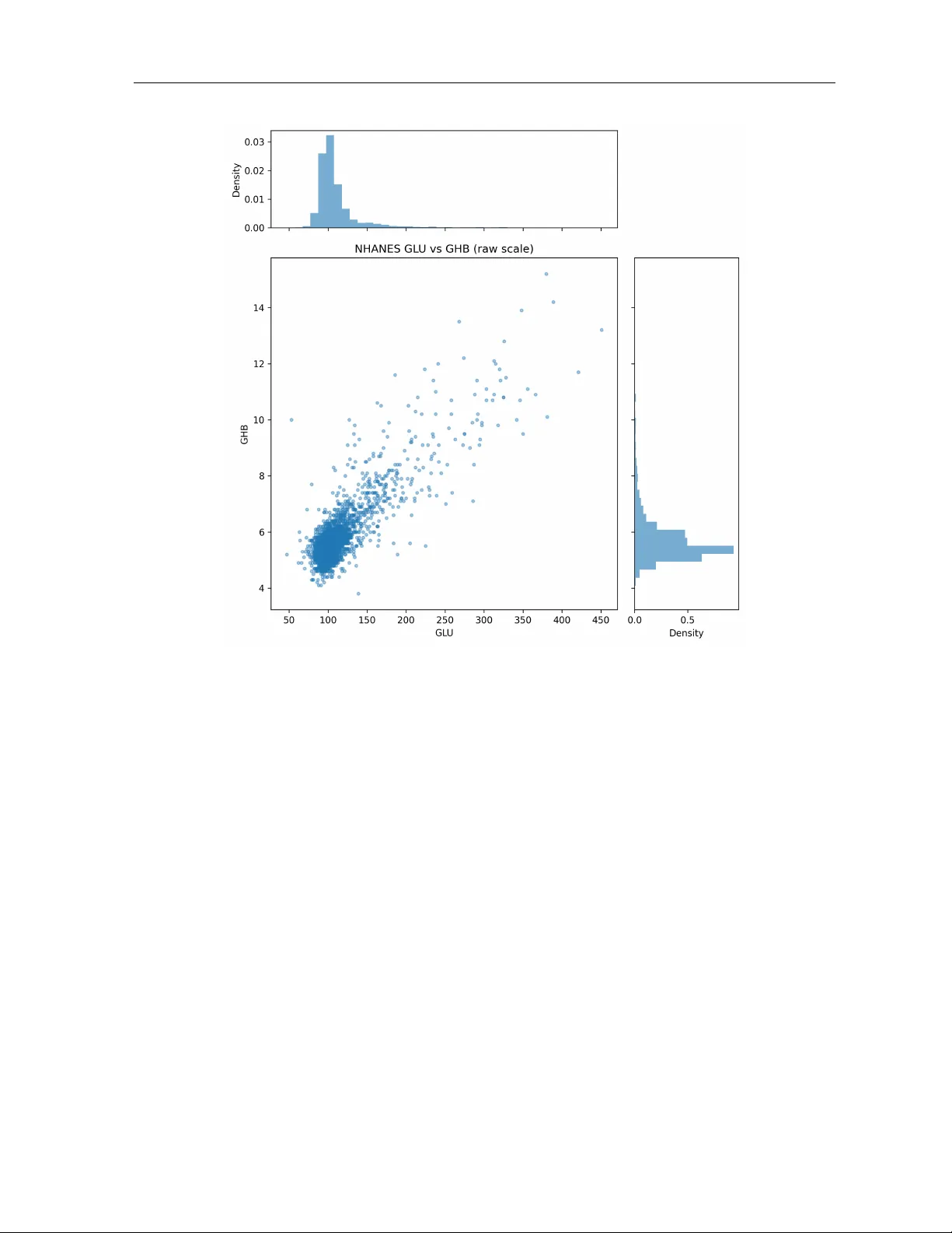
Ba y esian Inference for Join t T ail Risk in P aired Biomark ers via Arc himedean Copulas with Restricted Jeffreys Priors Agnideep Aic h 1 ∗ , Md Monzur Murshed 2 , Sameera Hew age 3 and Ashit Baran Aic h 4 1 Departmen t of Mathematics, Universit y of Louisiana at Lafa y ette, Lafa yette, LA, USA. 2 Departmen t of Mathematics and Statistics, Minnesota State Universit y , Mank ato, MN, USA 3 Departmen t of Physical Sciences & Mathematics, W est Lib ert y Universit y , W est Lib ert y , WV, USA 4 Departmen t of Statistics, F ormerly of Presidency College, Kolk ata, India Abstract W e prop ose a Ba y esian copula-based framew ork to quan tify clinically in terpretable joint tail risks from paired con tinuous biomarkers. After conv erting eac h biomark er margin to rank-based pseudo-observ ations, we mo del dep endence using one-parameter Arc himedean copulas and fo cus on three probabilit y-scale summaries at tail level α : the low er-tail joint risk R L ( θ ) = C θ ( α, α ), the upp er-tail joint risk R U ( θ ) = 2 α − 1 + C θ (1 − α, 1 − α ), and the conditional low er-tail risk R C ( θ ) = R L ( θ ) /α . Uncertain ty is quantified via a restricted Jeffreys prior on the copula parameter and grid-based posterior approximation, which in- duces an exact posterior for eac h tail-risk functional. In sim ulations from Cla yton and Gum b el copulas across m ultiple dep endence strengths, posterior credible interv als achiev e near-nominal cov erage for R L , R U , and R C . W e then analyze NHANES 2017–2018 fast- ing glucose (GLU) and HbA1c (GHB) ( n = 2887) at α = 0 . 05, obtaining tight p osterior credible interv als for b oth the dep endence parameter and induced tail risks. The results re- v eal mark edly elev ated extremal co-mov emen t relativ e to indep endence; under the Gumbel mo del, the posterior mean join t upper-tail risk is R U ( α ) = 0 . 0286, appro ximately 11 . 46 × the indep endence b enc hmark α 2 = 0 . 0025. Ov erall, the prop osed approac h provides a princi- pled, dep endence-a ware method for rep orting join t and conditional extremal-risk summaries with Bay esian uncertain ty quantification in biomedical applications. 1. In tro duction The join t b eha viour of paired contin uous biomarkers is of great in terest in medicine, reliability engineering and the so cial sciences. In a stress–strength mo del one measures the reliability of a comp onen t with strength X sub ject to a random stress Y through R = Pr( X > Y ); early w ork by Birnbaum formalised this quan tity and connected it with the Mann–Whitney statistic for t wo indep enden t samples [ Birnbaum , 1956 ]. The literature on estimating R is extensiv e and includes classical confidence b ounds [ Nandi and Aic h , 1994 ] as well as Bay esian tests based on a restricted parameter space[ Nandi and Aic h , 1996 ]. In biomedical applications one often wishes to assess join t abnormalit y risk for t wo biomarkers measured on the same individuals; for example, the probabilit y that b oth fasting glucose and HbA1c fall simultaneously in their ∗ Corresp onding author: Agnideep Aic h, agnideep.aich1@louisiana.edu , ORCID: 0000-0003-4432-1140 1 extremal regions is clinically meaningful. A direct interpretation of such extremal co-mov emen t is afforded by tail-risk functionals of the form R T ( θ ) = Pr θ { ( U, V ) ∈ T } for an appropriate tail region T and a dep endence parameter θ . When T corresponds to joint lo wer tails ( U ≤ α , V ≤ α ), join t upp er tails ( U ≥ 1 − α , V ≥ 1 − α ) or conditional lo wer tails ( U ≤ α giv en V ≤ α ), the resulting probabilities R L , R U and R C pro vide clinically interpretable summaries that are in v ariant to marginal transformations. T raditional correlation coefficients do not isolate b eha viour in the extremes and therefore ma y mask clinically relev an t tail dep endence. Copula models offer a principled w ay to separate marginal b eha viour from dep endence. Sklar’s theorem [ Sklar , 1959 ] states that ev ery m ultiv ariate distribution with contin uous margins can b e expressed as a copula applied to its marginal cum ulative distribution functions[ Nelsen , 2006 ]. The second edition of Nelsen’s monograph pro vides a comp endium of parametric copula families and discusses their properties and applications. T ail dep endence and measures of as- so ciation are treated systematically in that text; see also Jo e’s monograph for a comprehensive accoun t of multiv ariate dep endence structures[ Jo e , 1997 ]. In practice one often restricts atten- tion to one-parameter Archimedean copulas b ecause of their analytical tractability and ability to mo del either low er or upper tail dep endence. Among these, the Cla yton family exhibits strong low er-tail asso ciation whereas the Gumbel–Hougaard family captures positive upp er-tail dep endence. Go o dness-of-fit pro cedures and diagnostic to ols for copula mo dels are survey ed by Genest et al. [ 2009 ], who emphasise that common families such as Clayton, Gumbel, F rank and F arlie–Gumbel–Morgenstern are widely used in actuarial science, surviv al analysis and finance. Despite their suitabilit y for mo delling extremal co-mo vemen t, copulas hav e b een under-utilised in the stress–strength literature. Classical analyses assume either indep endence of X and Y or imp ose a specific biv ariate normal distribution; for example, Nandi and Aich [ 1994 ] deriv ed t wo-sided confidence b ounds for Pr( X > Y ) in biv ariate normal samples. Nandi and Aich [ 1996 ] prop osed a Bay esian h yp othesis test for reliability under a p ositiv e quadrant restric- tion, again assuming a particular parametric form. More recen t work has introduced sp ecific parametric biv ariate distributions via copulas: Kundu and Gupta [ 2011 ] constructed an abso- lutely contin uous biv ariate generalized exp onen tial distribution using the Clayton copula, while Domma and Giordano [ 2012 ] modelled the joint distribution of household income and consump- tion via a F rank copula to measure financial fragility . P atil et al. [ 2022 ] examined the impact of dep endence on R = Pr( Y < X ) when the margins are exp onen tial and compared estimation metho ds for sev eral copula families, including F arlie–Gumbel–Morgenstern, Ali–Mikhail–Haq and Gum b el–Hougaard. Outside of reliability , there is growing interest in expanding the class of Archimedean generators and developing robust estimators. Aic h et al. [ 2025a ] prop osed tw o new generator functions yielding copulas with flexible dep endence prop erties, and Aic h [ 2026 ] in tro duced a neural netw ork estimator that accurately reco vers copula parameters when classical lik eliho od metho ds b ecome unstable. In this paper, we develop a Ba yesian framew ork for clinically in terpretable tail-risk inference using Arc himedean copulas. By transforming eac h biomark er to the copula scale via rank-based pseudo-observ ations, our approac h isolates the dep endence structure from the margins. W e deriv e general generator-based iden tities for the copula densit y and its deriv atives, whic h are necessary for lik eliho od ev aluation and p osterior computation. A restricted Jeffreys prior is prop osed to mitigate impropriety at the b oundaries of the parameter space. Posterior summaries for θ are propagated through the tail-risk functionals R L , R U and R C to obtain Ba yesian credible in terv als that are easy to interpret in clinical terms. W e sp ecialise the metho dology to the Cla yton and Gumbel families to illustrate complemen tary low er- and upp er-tail b eha viour, v alidate the pro cedure in a simulation study , and apply it to NHANES data on fasting glucose 2 and HbA1c. Compared with existing reliability analyses, our contribution lies in (i) fo cusing on join t tail probabilities rather than Pr( X > Y ) alone; (ii) providing a general likelihoo d–based Ba yesian treatmen t for Archimedean copulas; and (iii) demonstrating how to quantify extremal co-mo vemen t in real data. Section 2 reviews related w ork. Section 3 presents the prop osed Ba yesian Arc himedean copula framework and the tail-risk functionals. Section 4 pro vides the clinical interpretation and the practical inference w orkflow. Section 5 rep orts sim ulation results. Section 6 presen ts the NHANES case study . Finally , Section 7 concludes and outlines future research directions. 2. Related w ork The probabilit y that a strength v ariable exceeds a stress v ariable, R = Pr( X > Y ), has long b een the cornerstone of reliabilit y analysis. The earliest con tributions assumed independence and normality , leading to closed-form expressions and asymptotic tests. Nandi and Aich [ 1994 ] constructed tw o-sided confidence b ounds for R under a biv ariate normal mo del. In a Bay esian setting, Nandi and Aich [ 1996 ] deriv ed a highest p osterior density credible set for R when X and Y follow indep enden t Gaussian distributions and the mean parameters are restricted to the positive quadrant. These early studies did not attempt to mo del dependence b ey ond the normal paradigm. Later w ork relaxed the distributional assumptions and introduced new parametric families to b etter capture dep endence. The absolutely contin uous biv ariate generalized exponential dis- tribution of Kundu and Gupta [ 2011 ] is an example; it is constructed using a Clayton copula to link marginal generalized exp onen tial distributions. Estimation of R under this mo del pro ceeds via classical lik eliho o d tec hniques. Domma and Giordano [ 2012 ] considered a F rank copula with Dagum marginal distributions to measure household financial fragilit y , sho wing that ne- glecting dep endence can ov erestimate risk. Both pap ers emphasise the flexibility of copulas for joining differen t marginal families. P atil et al. [ 2022 ] focused on the effect of dep endence when X and Y hav e exp onen tial margins. They deriv ed closed-form expressions for R for sev- eral p opular copulas and estimated the dep endence parameter using conditional lik eliho od and metho d-of-momen ts techniques. Their analysis remains within a frequen tist framework and do es not address tail-sp ecific risks. Copula theory itself has matured considerably . Comprehensiv e treatmen ts app ear in the monographs of Nelsen [ 2006 ] and Joe [ 1997 ], while Genest et al. [ 2009 ] surv ey go odness-of-fit tests and remark on the prev alence of Archimedean families in applied work. Researc hers con tinue to enrich the class of av ailable copulas and to develop improv ed estimators. F or example, the new Archimedean generators proposed b y Aic h et al. [ 2025a ] extend the range of tail dep endence beyond classical Clayton and Gum b el forms, and Aich [ 2026 ] demonstrate that neural net work estimators can outp erform maximum lik eliho od in difficult settings. Our w ork is complementary to these dev elopmen ts: w e pro vide general inference tools for tail-risk summaries that remain v alid regardless of the sp ecific Arc himedean generator and that can b e applied to newly prop osed families. Bey ond the classical stress–strength setting, copulas hav e recently been applied to super- vised learning tasks. Aic h et al. [ 2025d ] in tro duced a sup ervised filter that ranks predictors b y the Gum b el copula’s upp er-tail dep endence co efficien t and demonstrated impro ved feature selection for diab etes risk prediction. Aich et al. [ 2025b ] used Gaussian, Cla yton and Gumbel copulas to mo del the joint distribution of clinical and genomic risk scores in breast cancer and sho wed that a copula-based fusion of risk mo dels b etter stratifies patien t subgroups than linear 3 com binations. Neural copula densities underpin the deep copula classifier of Aich and Aich [ 2025 ], whic h ac hiev es Ba y es-consistent classification b y separating marginal estimation from dep endence mo delling. Finally , Aic h et al. [ 2025c ] prop osed CopulaSMOTE, using the A2 cop- ula to generate synthetic minority-class observ ations that preserve dependence in im balanced diab etes data. These studies highlight the v ersatility of copula metho ds in mac hine learning and data augmen tation, but they address feature selection, mo del fusion, classification and o versampling rather than inference for joint tail probabilities. Our fo cus is instead on Ba yesian quan tification of extremal co-mo vemen t via clinically interpretable tail-risk functionals. In summary , existing researc h on stress–strength mo dels and reliability has largely fo cused on estimating R = Pr( X > Y ) under sp ecific parametric assumptions and, more recently , on quan tifying the effect of dependence through particular copulas. None of the aforemen tioned w orks consider Ba yesian inference for joint tail probabilities R L , R U and R C or derive general lik eliho od identities for Arc himedean copulas. The present pap er fills this gap by developing a unified Ba yesian framew ork that conv erts rank-based pseudo-observ ations into clinically in ter- pretable tail-risk summaries, thereby extending the scop e of reliability analysis to applications where extremal co-mov ement is of primary concern. With this bac kground in place, w e next presen t our metho dological con tribution and the complete inference pip eline in Section 3 . 3. Metho dology This section presents the full metho dological pip eline used throughout the pap er: we in tro duce the copula-based dep endence model for paired con tin uous outcomes, define the clinically mo- tiv ated tail-risk functionals, derive the k ey Archimedean identities needed for likelihoo d-based inference, sp ecify the Bay esian mo del (Jeffreys and restricted Jeffreys priors) and the resulting p osterior for b oth θ and R T ( θ ), and then sp ecialize the general expressions to the Cla yton and Gum b el families used in our n umerical studies. 3.1 Setup, Notation, and T arget T ail-Risk F unctionals Let ( X i , Y i ) n i =1 b e i.i.d. observ ations from a contin uous biv ariate distribution. Let F X and F Y denote the marginal CDFs (known, or treated via pseudo-observ ations). Define the probability in tegral transforms U i = F X ( X i ) , V i = F Y ( Y i ) , so that ( U i , V i ) lie in (0 , 1) 2 and hav e uniform margins. Assume the dep endence is mo deled by a one-parameter copula family { C θ : θ ∈ Θ } with densit y c θ : P ( U ≤ u, V ≤ v ) = C θ ( u, v ) , c θ ( u, v ) = ∂ 2 ∂ u ∂ v C θ ( u, v ) . 3.1.1 T arget T ail-risk F unctionals W e consider tail-risk functionals of the copula parameter θ . R T ( θ ) = E θ [ g T ( U, V )] = Z 1 0 Z 1 0 g T ( u, v ) c θ ( u, v ) du dv , where ( U, V ) ∼ C θ and T ∈ { L, U, C } indexes the tail-risk functional: T = L (lo wer-tail join t risk), T = U (upp er-tail joint risk), and T = C (conditional lo wer-tail risk). 4 T ail-risk F unctionals Used in This W ork. Fix a tail level α ∈ (0 , 1) (e.g., α = 0 . 05). W e consider: R L ( θ ) = Pr θ ( U ≤ α, V ≤ α ) = C θ ( α, α ) , R U ( θ ) = Pr θ ( U ≥ 1 − α, V ≥ 1 − α ) = 1 − 2(1 − α ) + C θ (1 − α, 1 − α ) = 2 α − 1 + C θ (1 − α, 1 − α ) , R C ( θ ) = Pr θ ( U ≤ α | V ≤ α ) = Pr θ ( U ≤ α, V ≤ α ) Pr( V ≤ α ) = C θ ( α, α ) α . 3.2 Arc himedean Copulas, Key Iden tities, and Lik eliho o d 3.2.1 Arc himedean F orm A biv ariate Archimedean copula has the form C θ ( u, v ) = φ − 1 θ  φ θ ( u ) + φ θ ( v )  , where φ θ : (0 , 1] → [0 , ∞ ) is a gener ator satisfying: 1. φ θ (1) = 0, 2. φ θ is strictly decreasing and conv ex, 3. φ θ is twice contin uously differen tiable on (0 , 1) (for densities/deriv atives b elo w). W rite s θ ( u, v ) = φ θ ( u ) + φ θ ( v ) , t θ ( u, v ) = C θ ( u, v ) = φ − 1 θ ( s θ ( u, v )) . Then φ θ ( t θ ( u, v )) = s θ ( u, v ). 3.2.2 Deriv ation of ∂ C θ /∂ v W e differentiate the identit y φ θ ( t θ ( u, v )) = φ θ ( u ) + φ θ ( v ) with resp ect to v . Since u is constan t in this differentiation, ∂ ∂ v φ θ  t θ ( u, v )  = ∂ ∂ v φ θ ( v ) . Apply the chain rule to the left-hand side: φ ′ θ  t θ ( u, v )  · ∂ ∂ v t θ ( u, v ) = φ ′ θ ( v ) . Therefore, ∂ ∂ v C θ ( u, v ) = ∂ ∂ v t θ ( u, v ) = φ ′ θ ( v ) φ ′ θ  C θ ( u, v )  . (1) This is the fundamen tal identit y that generalizes the Cla yton-only deriv ative in the original draft. 5 3.2.3 Deriv ation of the Copula Density c θ ( u, v ) W e next derive c θ ( u, v ) = ∂ 2 C θ ( u, v ) / ( ∂ u ∂ v ). F rom the previous step, w e already ha ve ∂ ∂ u C θ ( u, v ) = φ ′ θ ( u ) φ ′ θ  C θ ( u, v )  . Differen tiate this with resp ect to v : ∂ 2 ∂ v ∂ u C θ ( u, v ) = ∂ ∂ v φ ′ θ ( u ) φ ′ θ  C θ ( u, v )  ! . Since φ ′ θ ( u ) do es not dep end on v , it is a constan t in this differentiation : ∂ 2 ∂ v ∂ u C θ ( u, v ) = φ ′ θ ( u ) · ∂ ∂ v 1 φ ′ θ  C θ ( u, v )  ! . Let h ( x ) = 1 /φ ′ θ ( x ). Then h ′ ( x ) = − φ ′′ θ ( x ) / ( φ ′ θ ( x )) 2 . By the chain rule, ∂ ∂ v h  C θ ( u, v )  = h ′  C θ ( u, v )  · ∂ ∂ v C θ ( u, v ) = − φ ′′ θ  C θ ( u, v )   φ ′ θ  C θ ( u, v )  2 · ∂ ∂ v C θ ( u, v ) . No w substitute ( 1 ): ∂ ∂ v h  C θ ( u, v )  = − φ ′′ θ  C θ ( u, v )   φ ′ θ  C θ ( u, v )  2 · φ ′ θ ( v ) φ ′ θ  C θ ( u, v )  . Th us, c θ ( u, v ) = ∂ 2 ∂ u ∂ v C θ ( u, v ) = − φ ′′ θ  C θ ( u, v )  φ ′ θ ( u ) φ ′ θ ( v )  φ ′ θ  C θ ( u, v )  3 . (2) Under the standard Archimedean conditions (decreasing φ ′ θ and conv ex φ θ ), c θ ( u, v ) ≥ 0. 3.2.4 Lik eliho o d for θ In practice, when F X and F Y are unkno wn, we use pseudo-observ ations b U i = r i n +1 and b V i = s i n +1 , where r i and s i are the ranks of X i and Y i among ( X 1 , . . . , X n ) and ( Y 1 , . . . , Y n ), resp ectiv ely , and we ev aluate the copula likelihoo d b y replacing ( U i , V i ) with ( b U i , b V i ). Giv en pseudo-observ ations ( U i , V i ) n i =1 , the copula likelihoo d is L ( θ ) = n Y i =1 c θ ( U i , V i ) , ℓ ( θ ) = log L ( θ ) = n X i =1 log c θ ( U i , V i ) , (3) where c θ can b e ev aluated using ( 2 ) (and simplified for particular families). 6 3.3 Ba y esian Specification 3.4 Fisher Information Define the p er-observ ation Fisher information [ W ang and Merkle , 2018 ] for θ b y I ( θ ) = E θ "  ∂ ∂ θ log c θ ( U, V )  2 # = − E θ  ∂ 2 ∂ θ 2 log c θ ( U, V )  , pro vided standard regularity conditions p ermit exchanging differentiation and in tegration. F or n i.i.d. observ ations, the Fisher information is I n ( θ ) = n I ( θ ). Practical computation of I ( θ ) for Cla yton and Gum b el. F or b oth copula families con- sidered in this pap er, we compute the Fisher information I ( θ ) n umerically on a grid of θ v alues, whic h is sufficien t for constructing the (restricted) Jeffreys prior. Recall I ( θ ) = E θ "  ∂ ∂ θ log c θ ( U, V )  2 # , ( U, V ) ∼ C θ . F or a given θ , we appro ximate the score function b y a finite difference, s θ ( u, v ) ≈ log c θ + h ( u, v ) − log c θ − h ( u, v ) 2 h , with a small step size h > 0, and then estimate the exp ectation b y Monte Carlo: I ( θ ) ≈ 1 M M X m =1 s θ ( U m , V m ) 2 , ( U m , V m ) M m =1 i.i.d. ∼ C θ . In the Clayton case, c θ ( u, v ) is ev aluated using the closed-form densit y in ( 10 ). In the Gum b el case, c θ ( u, v ) is ev aluated via the general Archimedean density formula ( 2 ) together with the Gum b el generator deriv ativ es φ ′ θ ( t ) and φ ′′ θ ( t ) given in ( 14 ). Finally , we set π J ( θ ) ∝ p I ( θ ) and apply the family-sp ecific truncations used throughout (Clayton: θ ∈ [ θ min , θ max ] with θ min > 0; Gum b el: θ ∈ [1 + ε, θ max ] with ε > 0), yielding the restricted Jeffreys prior in ( 4 ). 3.4.1 Jeffreys Prior and Restricted Jeffreys Prior The Jeffreys prior [ F raser et al. , 2010 ] is π J ( θ ) ∝ p I ( θ ) . If domain kno wledge or iden tifiability imp oses θ ∈ [ θ min , θ max ] ⊂ Θ, define the restricted Jeffreys prior [ Lartillot et al. , 2016 ] as π J R ( θ ) = p I ( θ ) 1 { θ min ≤ θ ≤ θ max } R θ max θ min p I ( t ) dt . (4) 7 3.5 P osterior Inference for T ail-Risk F unctionals 3.5.1 P osterior for θ F rom Bay es’ theorem, π ( θ | U , V ) = L ( θ ) π J R ( θ ) R θ max θ min L ( t ) π J R ( t ) dt ∝ L ( θ ) π J R ( θ ) , (5) where L ( θ ) is giv en by ( 3 ). 3.5.2 P osterior for a T ail-risk F unctional R T ( θ ) and Ba y es Estimator Under Squared Loss Since R T ( θ ) is a deterministic function of θ (e.g., R T ∈ { R L , R U , R C } ), its p osterior is induced b y π ( θ | data ). The Ba yes estimator under squared-error loss is the p osterior mean: b R T ,B = E  R T ( θ ) | U , V  = Z θ max θ min R T ( θ ) π ( θ | U , V ) dθ. The p osterior v ariance is V ar  R T ( θ ) | U , V  = Z θ max θ min R T ( θ ) 2 π ( θ | U , V ) dθ − b R 2 T ,B . 3.5.3 Large-sample Appro ximation The original draft attempted to b ound a Ba y es-risk quantit y using Fisher information for θ alone. The mathematically correct route for a functional R ( θ ) is: (i) p osterior normalit y for θ (Bernstein–v on Mises) [ Le Cam , 1953 , v an der V aart , 1998 ] and (ii) a delta-metho d transfer from θ to R ( θ ). Theorem 3.1 (Posterior delta-metho d for R T ( θ ) ) Assume: 1. The true p ar ameter θ 0 ∈ ( θ min , θ max ) lies in the interior (so trunc ation is asymptotic al ly ne gligible). 2. The lo g-likeliho o d is twic e differ entiable and satisfies standar d r e gularity c onditions for p osterior normality. 3. I ( θ 0 ) > 0 and R T ( θ ) is differ entiable at θ 0 . Then, c onditional ly on the data, √ n ( θ − b θ ) | U , V ⇒ N  0 , I ( b θ ) − 1  . (6) and c onse quently, √ n  R T ( θ ) − R T ( b θ )  | U , V ⇒ N  0 ,  R ′ T ( b θ )  2 I ( b θ ) − 1  . (7) wher e b θ c an b e taken as the MLE (or p osterior mo de; they c oincide asymptotic al ly). Her e, I ( b θ ) serves as a c onsistent asymptotic plug-in for the true information I ( θ 0 ) . In p articular, V ar  R T ( θ ) | U , V  =  R ′ T ( b θ )  2 n I ( b θ ) + o P ( n − 1 ) . (8) 8 Justification of Theorem 3.1 . W e outline the steps explicitly: 1. Under regularit y and θ 0 in terior, the p osterior for θ satisfies a Bernstein–v on Mises ap- pro ximation [ Le Cam , 1953 , v an der V aart , 1998 ]: √ n ( θ − b θ ) | data ⇒ N  0 , I ( b θ ) − 1  , whic h implies ( 6 ). 2. Apply a first-order T aylor expansion of R T ( θ ) ab out b θ : R T ( θ ) = R T ( b θ ) + R ′ T ( b θ ) ( θ − b θ ) + remainder . 3. The remainder is o P ( n − 1 / 2 ) under differentiabilit y and concen tration of θ around b θ . 4. Therefore, conditional on data, √ n  R T ( θ ) − R T ( b θ )  ≈ R ′ T ( b θ ) · √ n ( θ − b θ ) ⇒ N  0 ,  R ′ T ( b θ )  2 I ( b θ ) − 1  , whic h yields ( 7 ) and ( 8 ). 3.5.4 Credible In terv al for R T ( θ ) A conv enient asymptotic (1 − γ ) credible in terv al follo ws from ( 7 ): CI 1 − γ ( R T ) : R T ( b θ ) ± z 1 − γ / 2 | R ′ T ( b θ ) | q n I ( b θ ) , where z 1 − γ / 2 is the standard normal quan tile. (Exact highest p osterior densit y interv al (HPD) in terv als can b e computed b y numerically ev aluating the induced p osterior of R T ( θ ) using ( 5 ).) 3.6 Sp ecialization 1: Cla yton Copula (Lo wer-T ail Dep endence) 3.6.1 Generator, Copula, and Deriv ativ es The Clayton generator [ Clayton , 1978 ] is φ θ ( t ) = t − θ − 1 θ , θ > 0 . Compute deriv atives (step-by-step): φ ′ θ ( t ) = 1 θ · ( − θ ) t − θ − 1 = − t − θ − 1 , φ ′′ θ ( t ) = ( θ + 1) t − θ − 2 . The copula is C θ ( u, v ) =  u − θ + v − θ − 1  − 1 /θ . (9) Using ( 1 ), we derive ∂ C θ /∂ v explicitly . Let S ( u, v ) = u − θ + v − θ − 1 so C θ ( u, v ) = S ( u, v ) − 1 /θ . Differen tiate directly: ∂ ∂ v C θ ( u, v ) = ∂ ∂ v  S ( u, v ) − 1 /θ  = − 1 θ S ( u, v ) − 1 /θ − 1 · ∂ S ∂ v . 9 No w ∂ S ∂ v = ∂ ∂ v  v − θ  = − θ v − θ − 1 . Substitute: ∂ ∂ v C θ ( u, v ) = − 1 θ S ( u, v ) − 1 /θ − 1 ·  − θ v − θ − 1  = S ( u, v ) − 1 /θ − 1 v − θ − 1 . This matches the general iden tity ( 1 ). 3.6.2 Copula Densit y via The Archimedean Densit y Apply ( 2 ) with t = C θ ( u, v ): c θ ( u, v ) = − φ ′′ θ ( t ) φ ′ θ ( u ) φ ′ θ ( v ) ( φ ′ θ ( t )) 3 . Substitute φ ′ θ ( x ) = − x − θ − 1 and φ ′′ θ ( x ) = ( θ + 1) x − θ − 2 : c θ ( u, v ) = − ( θ + 1) t − θ − 2 · ( − u − θ − 1 ) · ( − v − θ − 1 ) ( − t − θ − 1 ) 3 . Compute signs: ( − u − θ − 1 )( − v − θ − 1 ) = u − θ − 1 v − θ − 1 , and ( − t − θ − 1 ) 3 = − t − 3 θ − 3 . Hence c θ ( u, v ) = − ( θ + 1) t − θ − 2 u − θ − 1 v − θ − 1 − t − 3 θ − 3 = ( θ + 1) u − θ − 1 v − θ − 1 t ( − θ − 2)+(3 θ +3) . Simplify the p o wer of t : ( − θ − 2) + (3 θ + 3) = 2 θ + 1 . Th us c θ ( u, v ) = ( θ + 1) u − θ − 1 v − θ − 1 t 2 θ +1 . Finally substitute t = C θ ( u, v ) = S ( u, v ) − 1 /θ : t 2 θ +1 =  S ( u, v ) − 1 /θ  2 θ +1 = S ( u, v ) − (2+1 /θ ) . Therefore, c θ ( u, v ) = ( θ + 1) ( uv ) − θ − 1  u − θ + v − θ − 1  − (2+1 /θ ) . (10) 3.6.3 T ail-risk F unctionals for Clayton F or the Clayton copula ( 9 ), the joint tail risks are R L ( θ ) = C θ ( α, α ) =  2 α − θ − 1  − 1 /θ , R U ( θ ) = 1 − 2(1 − α ) + C θ (1 − α, 1 − α ) = 2 α − 1 +  2(1 − α ) − θ − 1  − 1 /θ , R C ( θ ) = R L ( θ ) α . 10 3.7 Sp ecialization 2: Gum b el Copula (Upp er-T ail Dependence) 3.7.1 Generator and Copula The Gumbel generator [ Gumbel , 1960 ] is φ θ ( t ) = ( − log t ) θ , θ ≥ 1 . Let a ( u ) = ( − log u ) θ , b ( v ) = ( − log v ) θ , s ( u, v ) = a ( u ) + b ( v ) , t ( u, v ) = s ( u, v ) 1 /θ . Then the Gumbel copula is C θ ( u, v ) = exp  − t ( u, v )  = exp  −  ( − log u ) θ + ( − log v ) θ  1 /θ  . (11) 3.7.2 Deriv ativ e ∂ C θ ( u, v ) /∂ v via the Arc himedean Iden t it y F or an Archimedean copula C θ ( u, v ) = φ − 1 θ ( φ θ ( u ) + φ θ ( v )), ∂ ∂ v C θ ( u, v ) = φ ′ θ ( v ) φ ′ θ  C θ ( u, v )  . (12) F or the Gumbel family , φ θ ( t ) = ( − log t ) θ ( θ ≥ 1), so φ ′ θ ( t ) = θ ( − log t ) θ − 1 ·  − 1 t  = − θ ( − log t ) θ − 1 t . Substituting into ( 12 ) gives ∂ ∂ v C θ ( u, v ) = − θ ( − log v ) θ − 1 v − θ ( − log C θ ( u,v )) θ − 1 C θ ( u,v ) = C θ ( u, v ) v  − log v − log C θ ( u, v )  θ − 1 . (13) Since C θ ( u, v ) = exp  − (( − log u ) θ + ( − log v ) θ ) 1 /θ  , w e hav e − log C θ ( u, v ) =  ( − log u ) θ + ( − log v ) θ  1 /θ , and therefore ( 13 ) is equiv alent to ∂ ∂ v C θ ( u, v ) = C θ ( u, v ) s ( u, v ) 1 /θ − 1 ( − log v ) θ − 1 v , s ( u, v ) = ( − log u ) θ + ( − log v ) θ . 3.7.3 Densit y via the General Arc himedean F orm ula T o keep the deriv ations correct and readable, w e use ( 2 ): c θ ( u, v ) = − φ ′′ θ ( C θ ( u, v )) φ ′ θ ( u ) φ ′ θ ( v ) ( φ ′ θ ( C θ ( u, v ))) 3 . Compute φ ′ θ ( t ) and φ ′′ θ ( t ) (step-by-step). First, φ θ ( t ) = ( − log t ) θ ⇒ φ ′ θ ( t ) = θ ( − log t ) θ − 1 ·  − 1 t  = − θ ( − log t ) θ − 1 t . 11 No w differentiate again: φ ′′ θ ( t ) = − θ · d dt  ( − log t ) θ − 1 t  . Let A ( t ) = ( − log t ) θ − 1 and B ( t ) = 1 /t . Then ( AB ) ′ = A ′ B + AB ′ . Compute A ′ ( t ) = ( θ − 1)( − log t ) θ − 2 ·  − 1 t  = − ( θ − 1)( − log t ) θ − 2 t , B ′ ( t ) = − 1 t 2 . Therefore, d dt  ( − log t ) θ − 1 t  = A ′ B + AB ′ =  − ( θ − 1)( − log t ) θ − 2 t  · 1 t + ( − log t ) θ − 1 ·  − 1 t 2  . So d dt  ( − log t ) θ − 1 t  = − ( θ − 1)( − log t ) θ − 2 t 2 − ( − log t ) θ − 1 t 2 . Multiply by − θ : φ ′′ θ ( t ) = θ  ( θ − 1)( − log t ) θ − 2 t 2 + ( − log t ) θ − 1 t 2  = θ ( − log t ) θ − 2 t 2  ( θ − 1) + ( − log t )  . (14) Substitute ( 14 ) and φ ′ θ in to ( 2 ) to obtain an explicit (algebraic) closed form for c θ ( u, v ). 3.7.4 T ail-risk F unctionals for Gumbel F or the Gumbel copula ( 11 ), the joint tail risks are R L ( θ ) = C θ ( α, α ) = exp  − 2 1 /θ ( − log α )  = α 2 1 /θ , R U ( θ ) = 1 − 2(1 − α ) + C θ (1 − α, 1 − α ) = 2 α − 1 + exp  − 2 1 /θ  − log (1 − α )   = 2 α − 1 + (1 − α ) 2 1 /θ , R C ( θ ) = R L ( θ ) α . The next section pro vides a clinical in terpretation of the target tail-risk summaries and explains ho w the estimation-and-bo otstrap workflo w is applied in practice. 4. Clinical Application F ramew ork This section describ es ho w a copula-based dep endence model yields clinically interpretable sum- maries of joint abnormality risk for tw o contin uous biomarkers measured on the same individ- uals. W e quan tify uncertain ty using a Bay esian approach with a restricted Jeffreys prior, then v alidate the same pip eline in a con trolled simulation study (Section 5 ) and apply it to NHANES fasting glucose and HbA1c (Section 6 ). 12 4.1 F rom Biomark ers to Dep endence-only Data Let { ( X i , Y i ) } n i =1 b e paired biomark er measuremen ts. Because clinical units and marginal distri- butions differ across biomarkers, w e isolate dep endence by conv erting eac h margin to rank-based pseudo-observ ations: b U i = r i n + 1 , b V i = s i n + 1 , where r i and s i are the ranks of X i and Y i among ( X 1 , . . . , X n ) and ( Y 1 , . . . , Y n ), resp ectiv ely . This pro duces data on (0 , 1) 2 suitable for copula likelihoo d-based inference. 4.2 Clinically Meaningful T ail-risk Summaries Fix a tail level α ∈ (0 , 1); throughout we use α = 0 . 05. F or a fitted copula C θ , we summarize extremal co-mov ement via: R L ( θ ) = Pr θ ( U ≤ α, V ≤ α ) = C θ ( α, α ) , R U ( θ ) = Pr θ ( U ≥ 1 − α, V ≥ 1 − α ) = 2 α − 1 + C θ (1 − α, 1 − α ) , R C ( θ ) = Pr θ ( U ≤ α | V ≤ α ) = R L ( θ ) α . Here R L measures simultane ous extr eme-low risk, R U measures simultane ous extr eme-high risk, and R C is the conditional clinical risk of one biomarker b eing extreme-lo w giv en the other is extreme-lo w. 4.3 Ba y esian Model Fitting and Uncertain ty Quan tification W e consider t wo one-parameter Arc himedean copulas with complementary tail b eha vior: Cla y- ton (low er-tail dep endence) and Gumbel (upp er-tail dep endence). Let c θ ( · , · ) denote the copula densit y implied b y C θ . Using pseudo-observ ations ( b U i , b V i ), we form the copula log-lik eliho od ℓ ( θ ) = n X i =1 log c θ ( b U i , b V i ) . T o quantify uncertain ty in ( R L , R U , R C ), we adopt a Ba yesian p osterior π ( θ | b U , b V ) ∝ exp { ℓ ( θ ) } π ( θ ) , where π ( θ ) is a r estricte d Jeffr eys prior on a truncated parameter space: π ( θ ) ∝ p I ( θ ) I { θ ∈ [ θ min , θ max ] } , with I ( θ ) denoting Fisher information for θ and truncation c hosen to a void pathological tails while remaining asymptotically negligible. Sp ecifically , w e use a restricted Jeffreys prior with family-sp ecific support: for Clayton, θ ∈ [ θ min , θ max ] with θ min = 10 − 4 and θ max = 50; for Gum b el, θ ∈ [1 + ε, θ max ] with ε = 10 − 6 and θ max = 50. P osterior summaries for θ and the induced clinical risks ( R L ( θ ) , R U ( θ ) , R C ( θ )) are computed b y ev aluating the p osterior on a fine θ -grid and sampling from the resulting discrete approximation. 13 T able 1: Bay esian simulation results for the Clayton copula ( n = 500, R = 50, α = 0 . 05). Rep orted are the true tail-risk summaries, the av erage posterior mean across replicates, and empirical cov erage of 95% p osterior credible in terv als. θ true R L true R L p ost. mean R U true R U p ost. mean R C true R C p ost. mean 2 0.035377 0.035270 0.006821 0.006806 0.707549 0.705394 5 0.043528 0.043455 0.012032 0.011962 0.870551 0.869101 10 0.046652 0.046655 0.018484 0.018519 0.933033 0.933099 Co verage of 95% p osterior CIs: ( R L , R U , R C ) = (0.94, 0.94, 0.94), (1.00, 1.00, 1.00), (0.96, 0.96, 0.96). 4.4 Ho w to Read the Results A natural reference is the indep endence baseline: under indep endence, Pr( U ≤ α, V ≤ α ) = α 2 , Pr( U ≥ 1 − α, V ≥ 1 − α ) = α 2 . With α = 0 . 05, this baseline equals α 2 = 0 . 0025. V alues substantially larger than α 2 indicate elev ated join t-tail risk; posterior credible interv als quantify the uncertaint y in these clinically in terpretable summaries. Ha ving established the interpretation and Bay esian workflo w, the next section ev aluates finite- sample p erformance under con trolled data ge n erated from kno wn copula models. 5. Sim ulation Study W e v alidate the Bay esian estimation-and-inference pip eline under known ground truth: (i) sim- ulate i.i.d. samples from a sp ecified copula with parameter θ , (ii) compute the copula likelihoo d on pseudo-observ ations, (iii) form the restricted-Jeffreys p osterior for θ , (iv) induce posterior summaries for ( R L , R U , R C ) at α = 0 . 05, and (v) ev aluate frequentist co verage of 95% p osterior credible interv als across rep eated datasets. 5.1 Design F or eac h copula family (Clayton and Gumbel) and each parameter v alue θ ∈ { 2 , 5 , 10 } , w e generated R = 50 indep enden t datasets of size n = 500 from the target copula using a sampling algorithm from Genest and Rivest [ 1993 ]. In each replicate, since the data are generated directly on the copula scale ( U, V ) ∈ (0 , 1) 2 with uniform margins, w e apply the copula likelihoo d directly to ( U, V ) and compute the restricted-Jeffreys p osterior o ver θ on a grid. W e then propagated p osterior uncertaint y to obtain the p osterior mean and 95% credible interv al for each tail- risk summary R L ( θ ), R U ( θ ), and R C ( θ ) at α = 0 . 05. Cov erage is rep orted as the fraction of replicates in which the 95% credible interv al con tains the corresp onding true v alue. 5.2 Results Across b oth copula families, the p osterior concen trates around the true parameter v alues and the induced p osterior means for ( R L , R U , R C ) closely match their ground truth. Empirical co verage of 95% credible interv als is near nominal across the full grid, supp orting the prop osed Ba yesian uncertaint y quantification for clinically meaningful tail-risk summaries. Ov erall, these sim ulations supp ort tw o tak eaw ays. First, restricted-Jeffreys Bay esian inference reco vers θ accurately under correct mo del sp ecification. Second, p osterior credible in terv als 14 T able 2: Bay esian simulation results for the Gumbel copula ( n = 500, R = 50, α = 0 . 05). Rep orted are the true tail-risk summaries, the av erage posterior mean across replicates, and empirical cov erage of 95% p osterior credible in terv als. θ true R L true R L p ost. mean R U true R U p ost. mean R C true R C p ost. mean 2 0.014457 0.014411 0.030029 0.029935 0.289132 0.288220 5 0.032026 0.032038 0.042782 0.042783 0.640529 0.640751 10 0.040327 0.040325 0.046509 0.046507 0.806530 0.806494 Co verage of 95% p osterior CIs: ( R L , R U , R C ) = (1.00, 1.00, 1.00), (1.00, 1.00, 1.00), (0.92, 0.92, 0.92). pro vide near-nominal uncertain ty quan tification for clinically in terpretable tail risks in b oth tails, including the conditional risk R C . W e no w apply the iden tical Ba yesian procedure to NHANES biomarkers to quantify extremal co-mo vemen t in a p opulation sample. 6. NHANES Case Study: F asting Glucose and HbA1c In this section, w e apply the Bay esian copula-lik eliho od pro cedure with a restricted Jeffreys prior to NHANES 2017–2018 fasting glucose (GLU) and HbA1c (GHB), obtaining p osterior summaries and credible interv als for clinically interpretable tail-risk measures. 6.1 Data Construction and Exploratory Visualization W e analyzed publicly av ailable NHANES 2017–2018 lab oratory data for fasting plasma glucose and glycohemoglobin (HbA1c). W e obtained the fasting glucose file (GLU J) and the glycohe- moglobin file (GHB J), retained the v ariables SEQN , LBXGLU (glucose), and LBXGH (HbA1c), and merged the t w o files by SEQN to k eep participan ts with b oth measurements. After remo ving missing v alues, the final paired sample size was n = 2887. Figure 1 visualizes the raw-scale relationship b et ween GLU and GHB along with marginal histograms. The scatterplot sho ws a clear p ositiv e association, motiv ating dep endence mo deling b ey ond an indep endence assumption. 6.2 Ba y esian Copula Inference and T ail-risk Summaries at α = 0 . 05 W e con verted eac h biomarker margin to rank-based pseudo-observ ations ( b U i , b V i ) and fit Clayton and Gum b el copulas using the copula likelihoo d and the restricted Jeffreys prior. F or Gumbel, w e use a restricted Jeffreys prior on θ ∈ [1 + ε, θ max ] with θ max = 50. F or reference, the corresp onding lik eliho o d maximizers (MLEs) w ere ˆ θ MLE = 0 . 6636 (Cla yton) and ˆ θ MLE = 1 . 8904 (Gum b el); the Bay esian p osterior concentrates near these v alues. T able 3 rep orts the NHANES sample size and inference settings. T able 4 rep orts p osterior means and 95% credible interv als for the induced clinical tail risks at α = 0 . 05. Clinical interpretation of NHANES GLU–GHB results. With α = 0 . 05, the inde- p endence b enc hmark is α 2 = 0 . 0025. Under the Gumbel mo del, the p osterior mean joint upp er-tail risk is R U ( α ) = 0 . 02864 with a tight 95% credible interv al [0.02786, 0.02938], imply- ing that the probabilit y of simultaneously b eing in the top 5% of b oth GLU and GHB is ab out 0 . 02864 / 0 . 0025 ≈ 11 . 46 times larger than under indep endence. In contrast, Cla yton assigns comparativ ely small joint upp er-tail risk ( R U ( α ) ≈ 0 . 00402) but a larger joint lo w er-tail risk 15 Figure 1: NHANES GLU vs. GHB on the raw scale with marginal histograms. ( R L ( α ) ≈ 0 . 01953), reflecting the complementary tail behavior encoded by the t wo copula fami- lies. Finally , the conditional low er-tail risk R C ( α ) quantifies the probability that one biomarker is in its b ottom 5% given the other is in its b ottom 5%; p osterior uncertain ty for R C is rep orted in T able 4 . 6.3 P osterior Visualization of Clinical T ail Risks Figure 2 sho ws p osterior distributions of R L ( α ) and R U ( α ) at α = 0 . 05 under b oth copula mo dels, with v ertical lines indicating p osterior means and shaded regions indicating 95% credible in terv als. The t wo mo dels emphasize different extremal b eha viors: Clayton concentrates mass on larger R L (lo wer-tail co-mo vemen t), whereas Gum b el concentrates mass on larger R U (upp er- tail co-mov ement), consiste n t with T able 4 . In the next section, w e conclude by summarizing the main metho dological and empirical findings and outline promising directions for extending copula-based Ba y esian tail-risk inference to ric her dep endence mo dels and broader clinical settings. 16 T able 3: NHANES GLU–GHB analysis summary and Bay esian inference settings. Quan tity V alue Biomark er pair GLU–GHB Sample size n 2887 T ail level α 0.05 Indep endence baseline α 2 0.0025 Restricted Jeffreys truncation θ max 50 Cla yton MLE ˆ θ MLE (diagnostic) 0.6636 Gum b el MLE ˆ θ MLE (diagnostic) 1.8904 T able 4: NHANES GLU–GHB Bay esian p osterior summaries at α = 0 . 05 under Clayton and Gum b el copulas. Rep orted are p osterior means and 95% credible interv als (CrI) for θ and induced tail risks. Quan tity Cla yton Gum b el θ (p osterior mean) 0.6622 1.8893 θ (95% CrI) [0.5971, 0.7271] [1.8327, 1.9463] R L ( α ) mean 0.019533 0.013252 R L ( α ) 95% CrI [0.018127, 0.020883] [0.012616, 0.013880] R U ( α ) mean 0.004022 0.028640 R U ( α ) 95% CrI [0.003877, 0.004166] [0.027862, 0.029381] R C ( α ) mean 0.390661 0.265034 R C ( α ) 95% CrI [0.362542, 0.417653] [0.252313, 0.277604] 7. Conclusion and F uture W ork This pap er developed a Bay esian pip eline for clinically interpretable join t tail-risk assessment from paired contin uous biomark ers using one-parameter Arc himedean copulas. By transforming the data to rank-based pseudo-observ ations, the approac h isolates dep endence from marginal effects and yields inference that is comparable across biomarkers measured on different clinical scales. W e fo cused on three clinically motiv ated tail-risk summaries at a fixed tail lev el α : the lo wer-tail joint risk R L ( θ ) = C θ ( α, α ), the upp er-tail join t risk R U ( θ ) = 2 α − 1 + C θ (1 − α, 1 − α ), and the conditional lo wer-tail risk R C ( θ ) = R L ( θ ) /α . These functionals translate dependence mo deling in to probability-scale summaries that quan tify simultaneous and conditional extremal co-mo vemen t in a wa y that is directly interpretable in clinical terms. Metho dologically , w e derived the key Arc himedean iden tities needed for likelihoo d-based inference and expressed the copula densit y c θ ( u, v ) in a general generator-based form. W e then adopted a restricted Jeffreys prior to quantify uncertain ty in θ , and propagated posterior uncer- tain ty to obtain induced posterior summaries and credible interv als for the tail-risk quantities R T ( θ ). In addition, we clarified the correct large-sample appro ximation for tail-risk functionals through p osterior normality for θ and a delta-method transfer to R T ( θ ), providing a principled asymptotic v ariance expression that complemen ts the exact grid-based p osterior calculations. Empirically , the sim ulation study show ed that the restricted-Jeffreys Ba yesian pro cedure reco vers the dep endence parameter accurately under correct mo del sp ecification and yields near-nominal uncertain ty quan tification for the induced tail-risk summaries across a range of dep endence strengths for b oth Cla yton and Gumbel copulas. In the NHANES 2017–2018 case 17 Figure 2: Posterior distributions of R L ( α ) (left) and R U ( α ) (righ t) for NHANES GLU–GHB with α = 0 . 05 under Cla yton and Gumbel copulas. V ertical lines denote p osterior means; shaded regions denote 95% credible in terv als. study of fasting glucose (GLU) and HbA1c (GHB), the Ba y esian p osterior concentrated near the likelihoo d maximizers and produced tigh t credible in terv als for θ and the clinically mean- ingful tail risks. The results highlighted complemen tary extremal b eha viors consisten t with the kno wn tail prop erties of the tw o families: the Gum b el mo del emphasized joint upp er-tail co-mo vemen t, whereas the Clayton mo del emphasized joint low er-tail co-mov ement. T ogether, these results illustrate ho w copula-based Bay esian tail-risk inference can yield stable and clin- ically interpretable summaries of extremal dep endence, offering an informativ e alternative to indep endence baselines and correlation-based measures. Sev eral directions can strengthen and extend the prop osed framework. First, while we fo cused on tw o standard one-parameter Arc himedean families, the same inference pip eline can b e applied to other copula families (including additional Archimedean and rotated v arian ts) to capture a wider range of dep endence patterns that may arise across biomarker pairs. In particular, future w ork can in vestigate the use of more flexible copulas that can represent dep endence in b oth tails simultaneously , suc h as A 1 and A 2 copulas [ Aich et al. , 2025a , Aic h , 2026 ], within the same Bay esian tail-risk framework. Second, b ecause copula choice is rarely kno wn a priori, future work can incorp orate princi- pled mo del comparison and mo del a veraging across candidate copulas, rep orting tail-risk sum- maries that accoun t for uncertain ty in the copula family as w ell as uncertain ty in the dependence parameter. Relatedly , it is useful to develop and report dep endence-fo cused diagnostic c hecks that emphasize the tail regions most relev ant to the clinical question, ensuring that tail-risk conclusions remain well supp orted by the data. Third, many clinical applications in v olve more than tw o biomarkers measured jointly . Ex- tending from the biv ariate setting to d > 2 biomarkers can b e pursued using multiv ariate copula constructions such as vine copulas, enabling multiv ariate analogs of joint-tail probabilities (e.g., Pr( U 1 ≤ α, . . . , U d ≤ α ) or Pr( U 1 ≥ 1 − α, . . . , U d ≥ 1 − α )) and corresp onding Bay esian uncertain ty quantification. Finally , dep endence may v ary across subp opulations or o ver time, esp ecially in longitudinal biomark er studies. F uture work can allo w the copula parameter to dep end on cov ariates and/or time through regression-st yle or dynamic copula models, leading to subgroup-sp ecific or time- v arying tail-risk summaries. Additional practical extensions include sensitivit y analysis o v er the tail lev el α and linking join t tail-risk summaries to do wnstream clinical outcomes to ev aluate 18 their prognostic v alue and p oten tial role in decision supp ort. Ov erall, the prop osed Ba yesian copula framew ork pro vides a principled foundation for dep endence-a ware, clinically interpretable tail-risk summaries from paired biomarkers. Broad- ening the copula class, scaling to multiv ariate and longitudinal settings, and integrating mo del uncertain ty and clinically guided diagnostics are promising steps tow ard wider deploymen t in biomedical and public-health applications. Data Av ailabilit y The NHANES 2017–2018 data used in this study are publicly a v ailable from the U.S. Centers for Disease Con trol and Prev en tion (CDC). The biomark er measurements analyzed here, fasting plasma glucose (GLU) and glycohemoglobin/HbA1c (GHB), are provided as lab oratory data files for the 2017–2018 cycle and can be do wnloaded from the NHANES data p ortal (Laboratory comp onen t): h ttps ://w wwn. cdc. gov/ nchs /nha nes/ sear ch/d atap age. aspx ?Co m pone nt= L a boratory&Cycle=2017- 2018 . Co de Av ailabilit y All co de used in this w ork is av ailable at: https: //github.com/ag nivibes/bayesi an- copul a- tail- risk- biomarkers . Author Con tributions A.A. conceived the study , led the metho dological dev elopment, implemen ted the computational w orkflow, p erformed the simulation study and data analyses, and drafted the manuscript. M.M.M. contributed to clinical/biomark er interpretation and man uscript revision. S.H. con- tributed to the literature review and manuscript preparation. A.B.A. con tributed to the the- oretical developmen t of the prop osed metho dology and sup ervised the pro ject. All authors review ed and appro ved the final v ersion of the man uscript. References Agnideep Aic h. A robust neural net work framework for constrained parameter estimation in arc himedean copulas. Communic ations in Statistics – Simulation and Computation , 2026. doi: 10.48550/arXiv.2505.22518. Accepted. Agnideep Aic h and Ashit Baran Aich. Deep copula classifier: Theory , consistency , and empirical ev aluation. arXiv pr eprint , 2025. doi: 10.48550/arXiv.2505.22997. Agnideep Aich, Ashit Baran Aich, and Bruce W ade. Tw o new generators of archimedean copulas with their properties. Communic ations in Statistics – The ory and Metho ds , 54(17):5566–5575, 2025a. doi: 10.1080/03610926.2024.2440577. Agnideep Aich, Sameera Hewage, and Md Monzur Murshed. Copula based fusion of clinical and genomic machine learning risk scores for breast cancer risk stratification. arXiv pr eprint , 2025b. doi: 10.48550/arXiv.2511.17605. 19 Agnideep Aic h, Md Monzur Murshed, Sameera Hewage, and Amanda May eaux. Copulasmote: A copula-based o versampling approac h for imbalanced classification in diabetes prediction. arXiv pr eprint , 2025c. doi: 10.48550/arXiv .2506.17326. Agnideep Aic h, Md Monzur Murshed, Sameera Hew age, and Amanda Ma y eaux. A copula based sup ervised filter for feature selection in machine learning driven diab etes risk prediction. arXiv pr eprint , 2025d. doi: 10.48550/arXiv .2505.22554. Z. W. Birn baum. On a use of the mann–whitney statistic. In Jerzy Neyman, editor, Pr o c e e dings of the Thir d Berkeley Symp osium on Mathematic al Statistics and Pr ob ability , volume 1, pages 13–18. Universit y of California Press, Berkeley , 1956. Da vid G. Cla yton. A mo del for asso ciation in biv ariate life tables and its application in epidemi- ological studies of familial tendency in chronic disease incidence. Biometrika , 65(1):141–151, 1978. doi: 10.1093/biomet/65.1.141. Filipp o Domma and Sabrina Giordano. A stress–strength mo del with dep enden t v ariables to measure household financial fragility . Statistic al Metho ds & Applic ations , 21(3):375–389, 2012. doi: 10.1007/s10260- 012- 0192- 5. D. A. S. F raser, N. Reid, E. Marras, and G. Y. Yi. Default priors for ba yesian and frequentist inference. Journal of the R oyal Statistic al So ciety: Series B (Statistic al Metho dolo gy) , 72(5): 631–654, 2010. doi: 10.1111/j.1467- 9868.2010.00750.x. Christian Genest and Louis-P aul Riv est. Statistical inference pro cedures for biv ariate arc himedean copulas. Journal of the A meric an Statistic al Asso ciation , 88(423):1034–1043, 1993. Christian Genest, Bruno R ´ emillard, and David Beaudoin. Go o dness-of-fit tests for copulas: a review and a p o wer study . Insur anc e: Mathematics and Ec onomics , 44(2):199–213, 2009. doi: 10.1016/j.insmatheco.2007.10.005. Emil Julius Gum b el. Biv ariate exponential distributions. Journal of the Americ an Statistic al Asso ciation , 55(292):698–707, 1960. Harry Jo e. Multivariate Mo dels and Dep endenc e Conc epts . Chapman and Hall, London, 1997. doi: 10.1201/b13150. Debasis Kundu and Rameshw ar Gupta. Absolute con tinuous biv ariate generalized exp onen tial distribution. AStA A dvanc es in Statistic al Analysis , 95(2):169–185, 2011. doi: 10.1007 /s101 82- 010- 0151- 0. Nicolas Lartillot, Matthew J. Phillips, and F redrik Ronquist. A mixed relaxed clock mo del. Philosophic al T r ansactions of the R oyal So ciety B: Biolo gic al Scienc es , 371(1699):20150132, 2016. doi: 10.1098/rstb.2015.0132. Lucien Le Cam. On some asymptotic prop erties of maximum likelihoo d estimates and related ba yes’ estimates. University of California Public ations in Statistics , 1(11):277–330, 1953. S. B. Nandi and A. B. Aich. A note on confidence bounds for P ( X > Y ) in biv ariate normal samples. Sankhy¯ a: The Indian Journal of Statistics, Series B , 56:129–136, 1994. 20 S. B. Nandi and A. B. Aic h. Hyp othesis-test for reliabilit y in a stress–strength mo del, with prior information. IEEE T r ansactions on R eliability , 45(1):129–131, 1996. Roger B. Nelsen. An Intr o duction to Copulas . Springer Series in Statistics. Springer, New Y ork, second edition, 2006. doi: 10.1007/0- 387- 28678- 0. Dipak Patil, U. V. Naik-Nimbalk ar, and M. M. Kale. Effect of dep endency on the estimation of P [ Y < X ]. Austrian Journal of Statistics , 51(4):10–34, 2022. doi: 10.17713/ajs.v51i4.1293. Ab e Sklar. F onctions de r´ epartition ` a n dimensions et leurs marges. Public ations de l’Institut de Statistique de l’Universit ´ e de Paris , 8:229–231, 1959. A. W. v an der V aart. Asymptotic Statistics . Cambridge Series in Statistical and Probabilistic Mathematics. Cambridge Universit y Press, Cam bridge, 1998. ISBN 978-0-521-49603-2. Ting W ang and Edgar C. Merkle. merderiv: Deriv ative computations for linear mixed effects mo dels with application to robust standard errors. Journal of Statistic al Softwar e , 87(13): 1–16, 2018. doi: 10.18637/jss.v087.c13. 21