Structural grouping of extreme value models via graph fused lasso

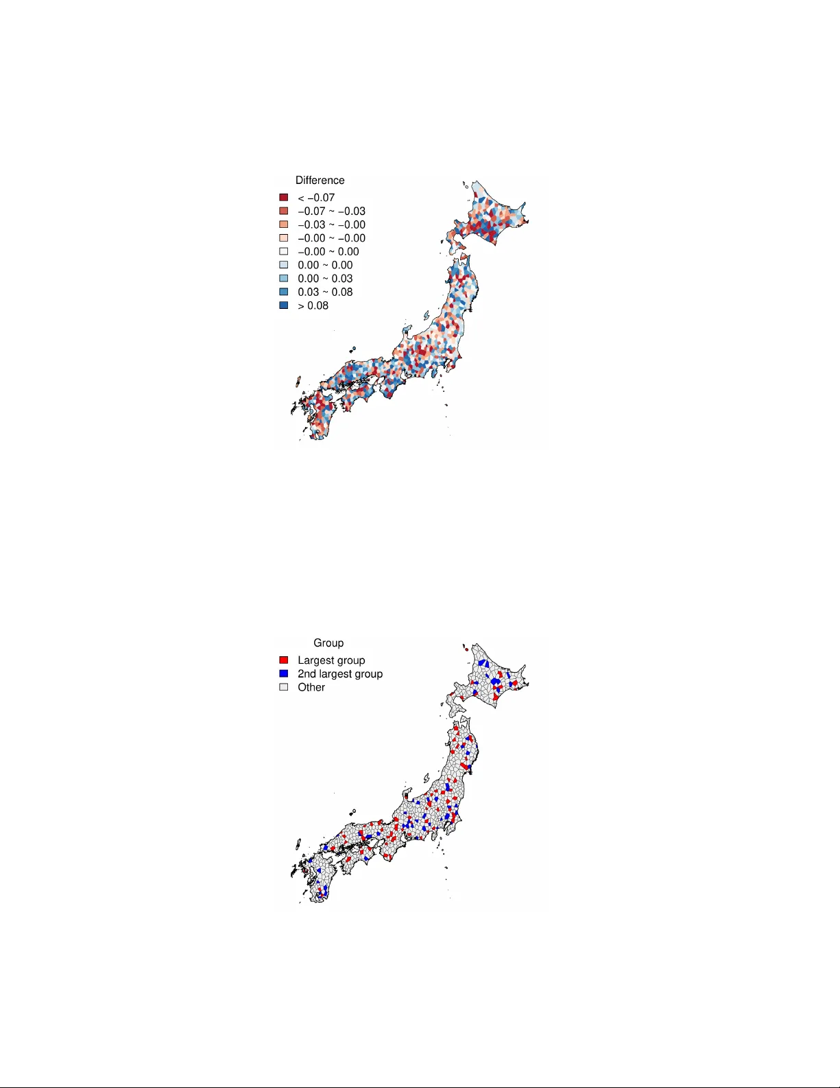
Structural grouping of extreme v alue mo dels via graph fused lasso T akuma Yoshid a 1 , 3 , K oki Momoki 2 , Shuichi Ka w ano 4 1 , 2 Gr aduate Scho ol of Scienc e and Engine ering, Kagoshima University 3 Data Scienc e and AI Innovation R ese ar ch Pr omotion Center, Shiga University 4 F aculty of Mathematics, Kyushu University Abstract The generalized P areto distribution (GPD) is a fundamental mo del for analyzing the tail b eha vior of a distribution. In particular, the shap e parameter of the GPD characterizes the extremal prop erties of the distribution. As describ ed in this pap er, w e prop ose a method for grouping shap e parameters in the GPD for clustered data via graph fused lasso. The prop osed metho d sim ultaneously estimates the model parameters and identiﬁes which clusters can b e grouped together. W e establish the asymptotic theory of the prop osed estimator and demonstrate that its v ariance is low er than that of the cluster-wise estimator. This v ariance reduction not only enhances estimation stabilit y but also pro vides a principled basis for iden tifying homogeneit y and heterogeneit y among clusters in terms of their tail b eha vior. W e assess the p erformance of the prop osed estimator through Monte Carlo simulations. As an illustrative example, our metho d is applied to rainfall data from 996 clustered sites across Japan. Keyw ords: Extreme v alue analysis; Generalized P areto distribution; Graph fused lasso; Clustered data; SCAD 1 INTR ODUCTION In man y ﬁelds of risk assessmen t, interest lies in predicting the tail b eha vior of a distribution rather than its mean or cen tral c haracteristics. Ho w ever, tail prediction is inherently diﬃcult and unstable b ecause of the inherent data sparsit y in extreme regions. T o construct eﬃcient esti- mators and prediction mo dels for tail b eha vior, we primarily examine the tail of the distribution rather than mo deling the en tire distribution. Extreme v alue theory (EVT) pro vides a theoretical foundation and statistical tools for mo deling tail b eha vior. As a commonly used EVT model, the generalized Pareto distribution (GPD) is ﬁtted to data exceeding a sp eciﬁed threshold and serv es as a mo del for extreme v alues. The GPD is characterized by t wo parameters: a shap e parameter and a scale parameter. The shap e parameter, also known as the extreme v alue index, determines the heaviness of the tail and the domain of attraction, whereas the scale parameter describ es the magnitude of threshold exceedance (de Haan and F erreira 2006). Estimation of shap e and scale parameters is t ypically conducted using the maxim um lik elihoo d method (e.g., Coles 2001). The fundamen tal theories of the maximum likelihoo d estimator were presen ted b y Smith (1987) and Drees et al. (2004). A typical example of a statistical problem using extreme v alue analysis is risk mo deling of climate data (e.g., Bousquet and Bernardara 2021). In general, climate data are a v ailable as clustered data b ecause these are observed daily at multiple observ ation sites. Then, the in teresting purp ose is the prediction of marginal distribution of eac h cluster and dep endence b et ween clusters. As describ ed herein, w e sp eciﬁcally examine the estimation of the marginal 1 distribution of each cluster. Then, the cluster-wise estimation of the parameters included in GPD is a classical approac h. Ho w ev er, for example, in climate data, one might consider that nearb y clusters (sites) tend to hav e similar features of the data. This tendency motiv ates us to explore the p ossibility of constructing more accurate estimators of the parameters of GPD b y incorp orating mutual information b et w een clusters. Actually , Hosking and W allis (1997) pro vided regional frequency analysis, whic h are p ooling data observ ed at sev eral clusters where the statistical b eha vior of the data is assumed to b e similar. Casson and Coles (1999) also studied the p o oling metho d of information of clusters in spatial extreme v alue mo dels. Einmahl et al. (2020) developed the nov el extreme v alue theory for p o oling clusters (and time dep endence). Ho w e v er, with those approac hes ab ov e, it is diﬃcult to choose the clusters to b e grouping when the n um b er of sites is v ery large. Dupuis et al. (2023) and Rohrbeck and T a wn (2023) ha v e also prop osed metho ds for clustering in the context of extreme v alue analysis. Dupuis et al. (2023) sp eciﬁcally examined blo ck maxima using the generalized extreme v alue distribution and prop osed a heuristic grouping metho d based on marginal similarity , selecting the b est mo del b y BIC. Their metho d migh t presen t scalability issues when the num b er of clusters is large b ecause of the exp onen tial gro wth in candidate mo dels. Rohrb ec k and T a wn (2023) considered clustering sites with extreme v alue inference. Their Bay esian approach join tly estimates marginal eﬀect, dependence structure, and cluster assignments, incorporating similarity in shap e and scale parameters as well as extreme dep endence. Details of other grouping methods in extreme v alue mo deling are presen ted by Rohrbeck and T a wn (2023). Consequen tly , extreme v alue mo deling with cluster grouping constitutes a useful framew ork for structurally c haracterizing tail b ehavior across clusters. As describ ed herein, w e provide the nov el metho d for simultaneous construction of accurate estimators of the parameters of the GPD in each cluster and grouping shape parameters in some clusters. Then, we aim to group the shap e parameter b etw een clusters b ecause it aﬀects the tail b eha vior and domain of attraction directly . Ho w ev er, grouping of scale parameters should b e treated carefully because the scale parameter b eha vior is closely related to b oth the threshold and the shap e parameter (de Haan and F erreira 2006, theorem 1.2.5). Consequen tly , when the scale parameter is group ed, w e should consider a grouping threshold in addition to the shape parameter (Section 3.2 herein). Ho w ever, it is diﬃcult b ecause the determination of a threshold is b ey ond the framework of estimation of parameters in GPD. Therefore, we will try to group only shap e parameters; not scale parameters. F rom this, the scale parameter represen ts the sp eciﬁc information of extreme v alue mo del for eac h cluster. Our prop osed metho d is conducted using a p enalized maxim um likelihoo d method. The lik elihoo d part consists of the lik eliho od based on GPD for each cluster. In the part of the p enalt y , we use the fused lasso p enalt y for the shap e parameters across clusters (Tibshirani et al. 2005). Then, if some of the shap e parameters can be regarded as equal, then the diﬀerence b et ween them is reduced to zero. In this situation, w e use the fused lasso on the graph of some connections b et ween eac h pair of clusters. Statistical methods using the idea of graph fused lasso ha ve b een dev elop ed b y She et al. (2010), Ke et al. (2015), W ang et al. (2016), T ang and Song (2016), W ang et al. (2018), and Hui et al. (2024). Ho w ever, a study examining a grouping method of the extreme v alue feature using graph fused lasso has not b een rep orted to date. By the sparsit y of the fused lasso p enalt y , the shap e parameters in m ultiple clusters are equal when these shap e parameters are inherently similar. If the shap e parameters in multiple clusters are detected to b e equal, then such clusters are said to hav e common extreme v alue distribution. One imp ortan t issue for applying the graph fused lasso is determination of which clusters are linked. If the num b er of clusters is J > 2, then the maxim um n umber of p ossible connections (i.e., edges on the graph) betw een clusters is J C 2 = J ( J − 1) / 2. F or example, if J = 1000, then w e ha ve J ( J − 1) / 2 ≈ 500 , 000, 2 whic h represents to o many connections to optimize the estimation. She (2010) p oin ted out that to o many p enalties engender unstable estimation or infeasible computation in graph fused lasso problem. Therefore, for application, it is necessary to reduce the num b er of edges of the graph appropriately . F or that reason, in our approac h, we use a user-sp eciﬁed graph of the connections b et ween clusters by prior analysis or information of data. F or example, for the climate data or spatial data, w e can consider the connection based on the distance betw een the lo cations of clusters. F or time series observed data, some dependence measure is also useful to decide the graph. After constructing the graph, we estimate the parameters using a p enalized maximum likeli- ho od approac h with a graph fused lasso p enalty . T o calibrate the p enalt y strength for eac h pair of clusters, we incorp orate the adaptiv e lasso framew ork prop osed by Zou (2006). Sp eciﬁcally , cluster-wise estimators are used as initial v alues for the shap e parameters. Subsequently , w e emplo y the ﬁrst deriv ativ e of a non-concav e penalty , such as SCAD (F an and Li 2001) or MCP (Zhang 2010), to construct adaptive weigh ts. This weigh ting mec hanism eﬀectively remov es the p enalt y for pairs of clusters for whic h initial estimates diﬀer considerably , even if they are con- nected in the sp eciﬁed graph. Consequen tly , b y adaptively reﬁning the graph structure through these weigh ts, the proposed join t estimation and clustering pro cedure impro v es computational eﬃciency and decreases estimation bias arising from inappropriate p enalization b et w een hetero- geneous clusters. F or this study , we establish the asymptotic theory of the prop osed adaptive graph fused lasso estimator and demonstrate that its v ariance is lo w compared to that of the cluster-wise estimator. This v ariance reduction not only enhances estimation stabilit y but also facilitates a principled iden tiﬁcation of homogeneit y and heterogeneit y among clusters in terms of their tail b eha vior. This paper is organized as explained b elo w. Section 2 presen ts reviews of the EVT and GPD. The prop osed grouping method of clusters is described in Section 3. Theoretical prop erties of the prop osed metho d are revealed in Section 4. A sim ulation study is conducted in Section 5, whereas a real data example is demonstrated in Section 6. Section 7 presents the salien t conclusions. In the Appendix, the technical lemmas and the pro of of theorems in Section 4 are presen ted. Additional studies of simulation and real data example are presented as supplemen tary materials. 2 GENERALIZED P ARETO DISTRIBUTION Let X 1 , . . . , X n ∈ R b e i.i.d. random v ariables with a distribution function F ( x ) = P ( X i < x ). First we deﬁne the domain of attraction of F . If there exists a constan t γ ∈ R and sequences a n ∈ R and b n > 0 , n ∈ N suc h that lim n →∞ P  max i X i − a n b n < z  = G γ ( z ) = exp[ − (1 + γ z ) − 1 /γ + ] , z > 0 , then the distribution function F is said to belong to the maxim um domain of attraction of G γ , as denoted b y F ∈ D ( G γ ), where ( x ) + = max { x, 0 } . The distribution function G γ is the so-called generalized extreme v alue distribution. W e next introduce the GPD. Let H ( x | γ ) = (1 + γ x ) − 1 /γ + . If γ = 0, then w e deﬁne H ( x | 0) = lim γ → 0 H ( x | γ ) = 1 − e − y . The function H ( x | γ ) is kno wn as the surviv al function of the GPD. According to Chapter 4 of Coles (2001), F ∈ D ( G γ ) if and only if lim w → x ∗ P ( X i > w + ξ w x | X i > w ) = lim w → x ∗ 1 − F ( w + ξ w x ) 1 − F ( w ) = H ( x | γ ) (1) 3 with some sequence ξ w > 0 of w ∈ R and x ∗ = sup { x : F ( x ) < 1 } . In fact, ξ w is not unique b ecause its b eha vior is determined only b y the limiting prop erty (de Haan and F erreira 2006, theorem 1.2.5). F rom (1), it is apparen t that for the random v ariable Y i = X i − w giv en some large w ∈ R , P ( Y i > y | Y i > 0) ≈ H  y ξ w     γ  . F rom the ab o ve, γ and ξ w resp ectiv ely represent the so-called shap e parameter and scale pa- rameter. Consequently , the tail b eha vior of the distribution function F can be dominated b y H ( y /ξ w | γ ). F or our analyses, we let h o ( y | γ , ξ w ) = ∂ 1 − H ( y /ξ w | γ ) ∂ y = 1 ξ w  1 + γ ξ w y  − 1 /γ − 1 + b e the densit y function asso ciated with H ( y /ξ w | γ ). Therefore, the log-likelihoo d function of ( γ , ξ w ) is deﬁned as n X i =1 I ( Y i > 0) log h o ( Y i | γ , ξ w ) . In fact, the samples with Y i < 0 are remo ved from the log-lik eliho o d function via the indica- tor function I ( · ) as non-extreme v alue data. By maximizing the log-lik eliho o d, w e obtain the maxim um likelihoo d estimator of ( γ , ξ w ). According to Drees et al. (2004), in the metho d presented ab o ve, the estimators of γ and ξ w are dep endent. Cha v ez-Demoulin and Davison (2005) examined reparameterization of the mo del to orthogonalize the maxim um lik eliho od estimators of shap e and scale parameters. Deﬁning σ w = ξ w ( γ + 1), we consider the pair ( γ , σ w ). Then, the surviv al function of the GPD is H  y ξ w | γ  = H  ( γ + 1) y σ w     γ  . Therefore, the densit y function of 1 − H with parameters ( γ , σ w ) b ecomes h ( y | γ , σ w ) = γ + 1 σ w  1 + γ ( γ + 1) σ w y  − 1 /γ − 1 + . (2) The log-likelihoo d function of ( γ , σ w ) is ℓ ( γ , σ w ) = n X i =1 I ( Y i > 0) log h ( Y i | γ , σ w ) . The maxim um likelihoo d estimator of ( γ , σ w ) is denoted by (˜ γ , ˜ σ w ). By similar argumen ts to those presen ted b y Smith (1987) and Drees et al. (2004), we can sho w that ( ˜ γ , ˜ σ w ) is distributed asymptotically as a normal distribution. Then, by reparameterization of the scale parameter, one can sho w that E  ∂ 2 log h ( Y i | γ , σ w ) ∂ γ ∂ σ w     Y i > 0  = 0 . Sho wing this implies that the asymptotic co v ariance matrix of ( ˜ γ , ˜ σ w ), which is obtained as the in v erse of Fisher-information matrix, is diagonal. Consequently , ˜ γ and ˜ σ w are asymptotically indep enden t. Throughout this pap er, GPD is parameterized using ( γ , σ w ) instead of ( γ , ξ w ). Finally , w e review the limiting b ehavior of σ w . When γ < 0, x ∗ is ﬁnite. The x ∗ can b e ﬁnite or inﬁnite for γ = 0. Ho w ev er, for the analyses presented in this paper, w e assume that 4 H ( x ) = 1 − e − x/σ with σ > 0 if γ = 0. Then, x ∗ = ∞ for also γ = 0. Under such a condition, according to Theorem 1.2.5 of de Haan and F erreira (2006), we ha v e        lim w →∞ σ w w = γ ( γ + 1) , γ > 0 , lim w → x ∗ σ w x ∗ − w = − γ ( γ + 1) , γ < 0 , lim w →∞ σ w = σ, γ = 0 . (3) The formula (3) sho ws that σ w is not unique, but the behavior dep ends on the γ and threshold w . 3 PR OPOSED METHOD 3.1 Clustered data W e let { ( X i 1 , . . . , X iJ ) : i = 1 , . . . , n } be J -v ariate random v ariables from the join t distribution F ( x 1 , . . . , x J ) = P ( X i 1 < x 1 , . . . , X iJ < x J ). Here, X ij , i = 1 , . . . , n, j = 1 , . . . , J is the i -th observ ation of j -th cluster. That is, the i -th ev ents for all clusters o ccur sim ultaneously . F or example, X ij is the observ ation at i -th day of j -th lo cation or site. Next, w e assume that X 1 j , . . . , X n,j are marginally distributed indep enden tly and iden tically as F j ( x j ) = P ( X ij < x j ) for j = 1 , . . . , J . In addition, w e presume that F j ∈ D ( G γ j ) , j = 1 , . . . , J . Similarly to Section 2, w e can establish the tail mo del of X ij using the GPD for eac h cluster j . That is, for each j , giv en threshold w j ∈ R , Y ij = X ij − w j is assumed to b e distributed as the GPD P ( Y ij > y | Y ij > 0) ≈ H (( γ j + 1) y /σ j,w j | γ j ) with auxiliary sequence σ j,w j > 0. As describ ed in this pap er, w e are interested in the extreme v alue inference of the marginal distributions for all clusters. Of course, it migh t b e suﬃcien t to ﬁt the GPD separately for eac h cluster. Ho wev er, for clustered data, constructing a mo del that incorp orates or shares information across clusters is an imp ortan t topic (Hosking and W allis 1997; Rohrb ec k and T awn 2023). In EVT, if the shap e parameters are equal across clusters, i.e., γ j = γ k = γ for j  = k , then b oth F j and F k b elong to the same domain of attraction, D ( G γ ). This sameness of domain implies p ooling information across clusters, which can lead to more stable estimates of the shape parameter and impro ve prediction of extreme v alue model. Therefore, w e intend to group the clusters based on the similarity of their shap e parameters γ 1 , . . . , γ J , which aims to improv e the marginal extreme v alue mo del for each cluster by incorp orating information from other clusters. In extreme v alue analysis for clustered data, the extreme dep endence betw een clusters is also in teresting topic. How ever, from copula theory , estimation of the dep endence structure and the marginal eﬀects are separable (Nelsen 2006; Genest and Segers 2009). Under this separability , the present study focuses on marginal inference for eac h cluster indep enden tly , without explicitly mo deling the extreme dep endence b et ween clusters. 3.2 Graph fused lasso p enalization T o group the shap e parameters ha ving common information, we use the graph fused lasso-t yp e p enalized (negativ e) log-likelihoo d metho d. Deﬁne γ = ( γ 1 , . . . , γ J ) ⊤ , σ = ( σ 1 , . . . , σ J ) ⊤ and the negative log-likelihoo d function as ℓ ( γ , σ ) = − J X j =1 n X i =1 I ( Y ij > 0) log h ( Y ij | γ j , σ j ) . 5 W e next deﬁne the graph fused lasso p enalt y . W e let G = ( V , E ) be a graph with the vertices V = { 1 , . . . , J } and unordered edges E = { e 1 , . . . , e M } for M > 0. The v ertices corresp ond to the index of clusters. Edges hav e the role of connection b y whic h clusters are linked. F or an y 1 ≤ m ≤ M , there exists k , j ∈ V suc h that e m = ( j, k ). The loss function of graph fused lasso (e.g., W ang et al. 2016) is deﬁned as ℓ F ( γ , σ ) = ℓ ( γ , σ ) + λ X ( j,k ) ∈ E v j,k | γ j − γ k | , (4) where λ > 0 is the tuning parameter and v j,k s are weigh ts. As describ ed in this pap er, the graph G is user-sp eciﬁed. As the weigh t, the typical choice is v j,k = 1, which indicates the original fused lasso p enalt y (Tibshirani et al. 2005). The weigh t type of adaptiv e lasso (Zou 2006) uses v j,k = 1 / | ˜ γ j − ˜ γ k | , where ˜ γ j and ˜ γ k represen t the cluster-wise estimates. As describ ed herein, we mainly use the deriv ative of folded-concav e type p enalt y . The w eigh t is deﬁned as v j,k = ρ λ,a ( | ˜ γ j − ˜ γ k | ) where ρ λ,a ( t ) , a > 0 is con tin uous except for the ﬁnite num b er of t and satisﬁes ρ λ,a ( t ) = 0 for | t | > aλ and lim t → 0+ ρ λ,a ( t ) = 1. As an example, the deriv atives of SCAD (F an and Li 2001) and MCP (Zhang 2010) are useful. The SCAD-t yp e ρ λ , whic h is the deriv ativ e of the original deﬁnition of the SCAD p enalty , is deﬁned as ρ λ,a ( t ) = sgn( t ) I ( | t | < λ ) + ( aλ − | t | ) a − 1 sgn( t ) I ( λ < | t | < aλ ) for the constant a > 0. Here, sgn( x ) is the signature of x . When | t | > aλ , w e obtain ρ λ,a ( t ) = 0, whic h implies that if | ˜ γ j − ˜ γ k | > aλ , then v j,k = 0. Then, the p enalt y of j -th and k -th cluster is remo v e d. Therefore, these cannot b e group ed as same v alue. Consequen tly , b y our metho d, the graph G is ﬁrst set b y users from pilot study or prior information of data. Secondly , the graph v alidit y is c heck ed b y the weigh t ρ λ,a ( · ). The prop osed metho d is fundamentally similar to the one-step lo cal linear approximation metho d (Zou and Li 2008) using cluster-wise estimator as the initial estimator. Similarly to the original method of SCAD and that presen ted b y Ke et al. (2015), w e can consider the SCAD p enalt y and can update the p enalt y along with the estimator. Ho w ev er, for our experiments, the results obtained using iterative metho d were quite similar to those obtained using one-step optimization. Sharing information across clusters may stablize the extreme v alue mo del. How ever, in the prop osed method, we do not consider grouping the scale parameters ( σ 1 , . . . , σ J ). F rom this, the diﬀerence b et w een clusters can also b e incorp orated. In other words, if scale parameter also group ed, it loses the sp eciﬁc information of extreme v alue mo del for each cluster. Moreo ver, in tro ducing an additional penalty for scale parameters complicates optimization of the ob jectiv e function. F or these reasons, we do not p erform grouping of the scale parameters when using the prop osed metho d. In that sense, our method is related to the model work ed b y Einmahl et al. (2020). 3.3 T uning parameter selection W e denote { ( ˆ γ j , ˆ σ j ) : j = 1 , . . . , J } as the minimizer of (4). Using the prop osed method (4), the selection of the tuning parameter λ is crucially important. F or this study , we use BIC-type criteria as BIC( λ ) = − 2 J X j =1 n X i =1 I ( Y ij > 0) log h ( Y ij | ˆ γ j , ˆ σ j ) + ( J + K ( λ )) log   J X j =1 n j   , 6 where for eac h j = 1 , . . . , J , n j = P n i =1 I ( Y ij > 0) denotes the eﬀective sample size for the j -th cluster, and K ( λ ) represents the n um ber of groups conducted by the shap e parameters. When λ = 0, the grouping does not proceeded. Therefore, K (0) = J . If λ → ∞ , then all γ j ’s are group ed as one parameter, which indicates K ( ∞ ) = κ ( G ), where κ ( G ) is the n um ber of connected comp onen ts from initial graph G . Ho wev er, when λ is very large, some clusters will b e forced to be group ed irrespective of the goo dness of ﬁt to the lik eliho o d. In that sense, the BIC ab o ve balances the go odness of ﬁt and the mo del complexity . In fact, in the BIC ab o v e, the term J log  P J j =1 n j  is related to the n umber of scale parameters. It is meaningless to select λ . A similar type of BIC w as used also b y Dupius et al. (2023). 3.4 Implemen tation T o solv e (4), w e use the alternating direction metho d of multipliers (ADMM). The general prop erties of ADMM are describ ed b y Bo yd et al. (2011). Letting D be M × J orien ted incidence matrix of the graph G with elemen ts {− 1 , 0 , 1 } , where M is the num b er of edge E , then for m = 1 , . . . , M , if e m = ( j, k ), the m -th ro w vector of D consists 1 for j -th element, - for the k -th element, and 0 otherwise, where the orientations of signs are arbitrary . W e next deﬁne the M -diagonal matrix V with ( m, m )-elemen ts ˜ v m = v j,k for e m = ( j, k ). That is, w e obtain V D γ = ( v j,k ( γ j − γ k ) , ( j, k ) ∈ E ) . Let ∥ · ∥ 1 b e L 1 -norm. Then, the loss function of (4) can be written as ℓ F ( γ , σ ) = ℓ ( γ , σ ) + λ ∥ V D γ ∥ 1 . The equality-constrained optimization problem is minimize ℓ ( γ , σ ) + λ ∥ V u ∥ 1 sub ject to D γ = u . Its augmented Lagrangian function is obtainable as ℓ F ( γ , σ , u , s ) = ℓ ( γ , σ ) + λ ∥ V u ∥ 1 + s ⊤ ( D γ − u ) + ρ 2 ∥ D γ − u ∥ 2 with the unkno wn v ector u , s ∈ R M and the additional tuning parameter (step size) ρ > 0. The optimization problem of ADMM can b e established as sho wn b elow. Letting ( γ (0) , σ (0) ) b e the initial estimator of ( γ , σ ), then the estimators ( γ ( t ) , σ ( t ) , u ( t ) , s ( t ) ) of parameters for t -step iteration are u ( t ) = argmin u { s ( t − 1) } ⊤ ( D γ ( t − 1) − u ) + ρ 2 ∥ D γ ( t − 1) − u ∥ 2 + λ ∥ V u ∥ 1 , s ( t ) = s ( t − 1) + ρ ( D γ ( t − 1) − u ( t ) ) , ( γ ( t ) , σ ( t ) ) = argmin ( γ , σ ) ℓ ( γ , σ ) + { s ( t ) } ⊤ ( D γ − u ( t ) ) + ρ 2 ∥ D γ − u ( t ) ∥ 2 . (5) Eac h element of u ( t ) : u ( t ) m is obtainable b y closed form as u ( t ) m = sgn ( D γ ( t − 1) ) m + s ( t − 1) m ρ !      ( D γ ( t − 1) ) m + s ( t − 1) m ρ      − λw m ρ ! + , m = 1 , . . . , M , 7 where ( D γ ( t − 1) ) m and s ( t − 1) m resp ectiv ely represen t the m -th elemen t of ( D γ ( t − 1) ) and s ( t − 1) . In our metho d, step size ρ is v aried in eac h iteration as ρ = ρ ( t ) b ecause the estimator is hea vily dep enden t on the choice of ρ . The step size ρ ( t ) is deﬁned b y the method of He et al. (2000) and W ang and Liao (2001), deﬁned as ρ ( t ) =    2 ρ ( t − 1) , ∥ η ( t − 1) ∥ > µ ∥ ξ ( t − 1) ∥ , 2 − 1 ρ ( t − 1) , ∥ ξ ( t − 1) ∥ > µ ∥ η ( t − 1) ∥ , ρ ( t − 1) , otherwise , where η ( t ) = D γ ( t ) − u ( t ) , ξ ( t ) = ρ ( t − 1) D ( γ ( t ) − γ ( t − 1) ) and µ > 0. F or Sections 5 and 6, w e used µ = 5. Roughly sp eaking, if the norm ∥ η ( t − 1) ∥ is large, then the constrain t D γ = u is not w ell satisﬁed, implying insuﬃcient sparsity in D γ . Therefore, the last term of (5) is emphasized b y increasing ρ ( t ) . How ever, a large norm ∥ ξ ( t − 1) ∥ implies p o or go o dness-of-ﬁt to the mo del. In this case, decreasing ρ ( t ) reduces the inﬂuence of the last term of (5). Consequently , dynamically up dating the step size ρ ( t ) balances the sparsit y of D γ and the go odness-of-ﬁt of the model. If the algorithm is stopp ed for t -th iteration, then w e deﬁne the estimator ( ˆ γ , ˆ σ ) = ( γ ( t ) , σ ( t ) ). The group ed clusters are identiﬁable by the zero elemen ts of ˆ u = D ˆ γ . 4 ASYMPTOTIC THEOR Y 4.1 General conditions T o in v estigate the theoretical prop erties of the prop osed estimator, some technical conditions m ust b e established. The general conditions are listed as follows to establish the asymptotic theory of the estimator. (C1) There exist constants γ ∗ , γ ∗ ∈ ( − 1 / 2 , ∞ ) such that γ ∗ < min j γ j < max j γ j < γ ∗ . (C2) F or j = 1 , . . . , J , w j → x ∗ j , n j → ∞ and n j /n P → 0 as n → ∞ . (C1) is the standard condition of the GPD. If the shape parameter is less than − 1 / 2, then the Fisher information matrix based on GPD is w ell kno wn not to b e p ositiv e deﬁnite, whic h implies that the shap e parameter estimator is unstable. Consequently , γ ∗ > − 1 / 2 is important. (C2) is also standard in the asymptotic analysis in the EVT. Actually from (C2), the eﬀective sample size n j can be regarded as the in termediate order sequence in the EVT (de Haan and F erreira 2006, c hap. 2). In addition, we state the conv ergence rate of the distribution function conv erges to GPD. for F j ∈ D ( G γ j ), w e no w assume that, for the sequence of threshold w j , there exists an auxiliary function α j ( w j ) satisfying α j ( w j ) → 0 as w j → x ∗ j := sup { x : F j ( x ) < 1 } such that for any x > 0, lim w j → x ∗ j       1 − F j ( w j + x ) 1 − F j ( w j ) − H (( γ j + 1) x/σ j,w j | γ j ) α j ( w j )       = O (1) . (6) The condition (6) is detailed as (A1) given in App endix. This condition is closely related to the second-order condition in Extreme V alue Theory (EVT) (e.g., de Haan and F e rreira, 2006, Chapter 2) and is essential for characterizing the asymptotic bias of estimators in extreme v alue mo dels. How ever, since the primary fo cus of this study is not bias reduction, we emplo y the simpliﬁed notation ab o v e. Sp eciﬁcally , in Theorems 1 and 2, we adopt a v ariance-dominated assumption, where the term α j ( w j ) is assumed to v anish at a suﬃcien tly fast rate. 8 4.2 Oracle estimator T o clarify b eneﬁts of the prop osed grouping shap e parameter metho d, w e ﬁrst show the asymp- totic result of the estimator of shap e parameter under the condition that grouping is already done. Let A b e the index set of one of the true groups. F or simplicity , we write γ = γ j , j ∈ A . That is, for all j ∈ A , F j ∈ D ( G γ ). Without loss of generality , w e can assume that A = { 1 , . . . , J } . W e then construct the estimator { ˆ γ , ˆ σ j : j ∈ A} as the maximizer of ℓ A ( γ , σ 1 , . . . , σ J ) = X j ∈A n X i =1 I ( Y ij > ω j ) log h ( Y ij | γ , σ j ) . Letting n A = P j ∈A n j , we can then obtain the follo wing theorem. Theorem 1. Supp ose that (C1) and (C2) , and n 1 / 2 A max j ∈A α j ( w j ) → 0 . Then, as n → ∞ , { n A } 1 / 2 ( ˆ γ − γ ) D − → N (0 , ( γ + 1) 2 ) and n 1 / 2 j  ˆ σ j σ j,w j − 1  D − → N (0 , 2 γ + 1) , j ∈ A . F urthermor e, for any j ∈ A , { n A } 1 / 2 C ov (ˆ γ , ˆ σ j ) → 0 as n → ∞ . F rom Theorem 1, is readily apparent that the rate of conv ergence of the estimator ˆ γ is higher than that of eac h ˜ γ j , j ∈ A if A con tains at least t wo indices of clusters. Consequently , by grouping shap e parameters among clusters, the accuracy of the estimator of the shape parameter is increasing drastically . W e also ﬁnd that the grouping shap e parameter do es not aﬀect to the asymptotic rate of the scale parameter. How ever, to obtain the conﬁdence in terv al of σ j , it is necessary to estimate γ , which app ear as the standard deviation of ˆ σ j . Therefore, the accurate estimation of γ also has a go od inﬂuence on prediction of the scale parameter. W e brieﬂy describe the relation b et ween the group ed estimator ˆ γ and the cluster-wise esti- mators ˜ γ j , j ∈ A . The likelihoo d function of the GPD is well kno wn to b e asymmetric with resp ect to the shap e parameter (and also with respect to the scale parameter). Sp eciﬁcally , for eac h j , the lik eliho od decreases muc h more rapidly when the shap e parameter mov es tow ard smaller v alues than when it mov es to ward larger v alues around the MLE ˜ γ j . As a consequence, when shap e parameters are group ed across clusters, the group ed estimator tends to b e shifted to ward larger v alues to a void a great loss in likelihoo d. In other words, the set { j ∈ A : ˆ γ > ˜ γ j } tends to be large. This mec hanism leads to a more conserv ativ e model for man y clusters. In application, it is interesting to in vestigate the probabilit y of a rare ev ent o ccurring, P ( X ij > x ) for x > w j , instead of the estimator of parameters itself. F rom GPD mo deling, w e hav e P ( X ij > x ) = P ( X ij > x | X ij > w j ) P ( X ij > w j ) ≈ H ( x − w j | γ j , σ j ) P ( X ij > w j ). Therefore, we can ev aluate P ( X ij > x ) by replacing ( γ , σ j ) with its estimator. W e are also in terested in ev aluating the quantile of X ij at region of extreme v alue, which is called the return lev el. F or an y τ ∈ (0 , 1), the τ -th return lev el of X ij is deﬁned as R ( τ ) = inf { t : P ( X ij > t ) < τ } . If τ < P ( X ij > w j ), then the contin uity of H yields that R ( τ ) = R ( τ | γ , σ j ) ≈ { t : H ( y | γ , σ j ) P ( X ij > w j ) = τ } = w j + σ j γ ( γ + 1) (  τ P ( X ij > w j )  − γ − 1 ) . 9 W e write ξ j = P ( X ij > w j ). Then, w e obtain ˆ ξ j = n j /n and √ n ( ˆ ξ j − ξ j ) D → N (0 , ξ (1 − ξ )). Because R dep ends on ( γ , σ j , ξ j ), the return lev el can b e estimated b y replacing unknown parameters with these estimators. By the delta metho d, w e obtain R ( τ | ˆ γ , ˆ σ j , ˆ ξ j ) ≈ R ( τ | γ , σ j , ξ j ) + R γ ( τ | γ , σ j , ξ j )( ˆ γ − γ ) + R σ ( τ | γ , σ j , ξ j )( ˆ σ j − σ j ) + R ξ ( τ | γ , σ j , ξ j )( ˆ ξ j − ξ j ) , where R γ ( τ | γ , σ j , ξ j ) = ∂ R ( τ | γ , σ j , ξ ) /∂ γ , R σ ( τ | γ , σ j , ξ j ) = ∂ R ( τ | γ , σ j , ξ j ) /∂ σ j , and R ξ ( τ | γ , σ j , ξ j ) = ∂ R ( τ | γ , σ j , ξ ) /∂ ξ j (see Section 4.3.3 of Coles 2001). Letting z p b e the 100(1 − p )% quantile of standard normal distribution such that P ( Z > z p ) = p for Z ∼ N (0 , 1), then from Theorem 1, the 100(1 − p )% conﬁdence interv al of R ( τ | ˆ γ , ˆ σ j ) is obtained as R ( τ | ˆ γ , ˆ σ j ) ± z p/ 2 s ˆ R 2 γ ( ˆ γ j + 1) 2 n A + ˆ R 2 σ ˆ σ 2 j (2 ˆ γ + 1) n j + ˆ R 2 ξ ˆ ξ j (1 − ˆ ξ j ) n , (7) where ˆ R γ = R γ ( τ | ˆ γ , ˆ σ j , ˆ ξ j ), and deﬁnitions of ˆ R σ , ˆ R ξ are similar. When the shap e parameters are not group ed, the term n A in (7) is replaced by n j . Consequently , the conﬁdence interv al obtained from the grouped estimator b ecomes shorter than that from the cluster-wise estimator, indicating that the estimation error of the return level is reduced. Actually , the return level R ( τ | γ , σ ) dep ends exp onen tially on the shap e parameter γ , whereas it dep ends linearly on the scale parameter σ . As a result, the sensitivit y of R ( τ | γ , σ j ) to γ is muc h greater than to σ j . In (7), the rate of ˆ γ , n A , which is larger than n j (rate of cluster-wise estimator), helps stabilize the b ehavior of R γ . Theorem 1 is useful if grouping is correct. How ever, Theorem 1 is only a theoretical result b ecause w e are unable to detect A completely in practice. As explained in the following section, w e establish the asymptotic results obtained using the proposed estimator that creates a new group of clusters by graph fused lasso. 4.3 Graph fused lasso estimator Let A 1 , . . . , A K b e the index sets of true groups of shap e parameters such that for k = 1 , . . . , K , if α, β ∈ A k , w e obtain γ α = γ β =: γ and F α , F β ∈ D ( G γ ). When A j = { j } and K = J , the distributions for all c lusters belong to a domain of attraction with diﬀeren t shap e parameters. The cluster-wise estimator is obtained under this condition. As describ ed in this pap er, w e generally assume that K < J . The penalty in (4) can b e expressed as λ X ( j,k ) ∈ E v j,k | γ j − γ k | = λ 2 J X j,k =1 c j,k v j,k | γ j − γ k | where c j,k = 1 if there exists m such that e m = ( j, k ), and c j,k = 0 if there is no edge b et w een indices j and k . Therefore, w e obtain c j,k = c k,j and c j,j = 0 for j, k = 1 , . . . , J . The term 1/2 ab o ve is absorbed in the tuning parameter λ . Let G k = {A k , E k } b e the subgraph induced by the set of no des A k , where E k = { ( i, j ) ∈ A k × A k : c i,j = 1 } . Here, G and G k are undirected graphs. Then the sets B k,ℓ for ℓ = 1 , . . . , L k are deﬁned as presented b elo w. 1. B k, 1 , . . . , B k,L k are the distinct connected components of the subgraph G k . 10 2. B k, 1 , . . . , B k,L k satisfy L k [ ℓ =1 B k,ℓ = A k and B k,s ∩ B k,t = ∅ for s  = t. F or example, w e assume that A 1 = { 1 , 2 , 3 , 4 , 5 , 6 } and c 1 , 2 = c 2 , 3 = 1, c 1 , 3 = 0, c 4 , 5 = 1, c j, 4 = c j, 5 = 0 for j = 1 , 2 , 3, and c i, 6 = 0 for i = 1 , . . . , 5. Then, the graph is G 1 = ( A 1 , E 1 ) with E 1 = { (1 , 2) , (2 , 3) , (4 , 5) } . Subsequently , we can construct B 1 , 1 = { 1 , 2 , 3 } , B 1 , 2 = { 4 , 5 } and B 1 , 3 = { 6 } . It is notew orthy in this case that γ 1 = · · · = γ 6 although B 1 ,i ∩ B 1 ,j = ∅ for i, j = 1 , 2 , 3 ( i  = j ). The ob jectiv e loss function (4) can be written as ℓ F ( γ , σ ) = ℓ ( γ , σ ) + λ K X k =1 L k X ℓ =1 X i,j ∈B k,ℓ c i,j v j,k | γ i − γ j | + λ X ( i,j ) ∈A ∗ c i,j v j,k | γ i − γ j | , (8) where A ∗ = { ( α, β ) | ∃ k , h ( k  = h ) s . t . α ∈ A k and β ∈ A h } . F or ( i, j ) ∈ A ∗ if c i,j = 1, meaning that the link of γ i and γ j is mis-speciﬁed. Because the graph is user-sp eciﬁed, it do es not guaran tee that clusters sharing the same v alue of shap e parameter are link ed correctly . In other words, it is diﬃcult to pro duce a graph to connect all clusters in A k for k = 1 , . . . , K . Therefore, the set A ∗ , whic h indicates the misconnection, is generally non-empty . If w e w an t to mak e the graph so that L k = 1 and B k, 1 = A k for k = 1 , . . . , K , then w e hav e no c hoice but to consider a complete graph that includes all p ossible pairs of clusters. How ever, the complete graph engenders hea vy tasks of computation (She 2010), rendering its use unrealistic in practice. W e further let γ oracle = ( γ B k,ℓ , ℓ = 1 , . . . , L k , k = 1 , . . . , K ). Then, the loss function for oracle situation is ℓ oracle ( γ oracle , σ ) = − K X k =1 L k X ℓ =1 X j ∈B k,ℓ n j X i =1 log h ( Y ij | γ B k,ℓ , σ j ) . (9) Then, the estimator obtained b y minimizing ℓ oracle is deﬁned as ˆ γ oracle = ( ˆ γ B k,ℓ , ℓ = 1 , . . . , L k , k = 1 , . . . , K ) and ˆ σ oracle = ( ˆ σ B k,ℓ ,j , j ∈ B k,ℓ , ℓ = 1 , . . . , L k , k = 1 , . . . , K ) The asymptotic property of ( ˆ γ B k,ℓ , ˆ σ B k,ℓ ,j ) is obtained using theorem 1 with the true set B k,ℓ . Whether the prop osed estimator attains the oracle estimator or not is important. The follo wing theorem shows suc h an eﬃcient property of the estimator. Before stating the theorem, w e consider the following conditions. (C3) There exists δ > 0 suc h that min j  = k min α ∈A j ,β ∈A k | γ α − γ β | > δ . (C4) The weigh t function p λ,a ( · ) is a monotonically decreasing function, lim t → +0 p λ,a ( t ) = 1 and p λ,a ( t ) = 0 for t ≥ aλ with λ, a > 0. W e deﬁne n B k,ℓ = P j ∈B k,ℓ n j for ℓ = 1 , . . . , L k , k = 1 , . . . , K . 11 Theorem 2. Supp ose that (C1) – (C4) , and for ℓ = 1 , . . . , L k , k = 1 , . . . , K , n 1 / 2 B k,ℓ max j ∈B k,ℓ α j ( w j ) → 0 as n → ∞ . F urthermor e, supp ose that λ satisﬁes nλ → ∞ and max k,ℓ |B k,ℓ | / ( nλ ) → 0 . Then, ℓ F ( γ , σ ) has a strictly lo c al minimizer ( ˆ γ , ˆ σ ) such that ˆ γ = ˆ γ oracle , ˆ σ = ˆ σ oracle with pr ob ability tending to one. F rom Theorems 1 and 2, it is readily apparen t that the asymptotic rate of the v ariance of the prop osed estimator is faster than that of the cluster-wise estimator. This result is aﬀected strongly b y the condition that n 1 / 2 B k,ℓ max j ∈B k,ℓ α j ( w j ) → 0 in Theorem 2. This assumption indicates that the asymptotic bias of the es timator is suﬃcien tly small. One migh t think that this condition is strong, but this is justiﬁed in the con text of our grouping metho d. In practice, if the large v alue of the threshold is used, then the bias b ecomes small. F or the cluster-wise estimator, the very large v alue of threshold leads to a large v ariance b ecause the eﬀectiv e sample size becomes small. By contrast, using our method, such a diﬃcult y of the small eﬀective sample size would be co v ered b y grouping clusters. F or example, the conﬁdence in terv al of the parameters in GPD and return lev el is constructed traditionally under the condition that the bias is assumed to b e zero (Coles 2001, sect. 3). The grouping of clusters in our metho d helps to construct the accurate conﬁdence interv al. 5 SIMULA TION W e conducted the Monte Carlo sim ulation to inv estigate the ﬁnite sample p erformance of the prop osed estimator. The adv an tage of the proposed grouping metho d is reducing the v ariance of the estimator compared with cluster-wise estimator. T o conﬁrm this b eneﬁt, in this simulation, w e generate data from each cluster using the GPD with some dep endence b et w een clusters. The data were generated according to the following pro cedure. First, we indep enden tly obtained Z 1 , 1 , . . . , Z n, 1 ∼ N (0 , 1), which are used to create the data for the ﬁrst cluster. Next, the j - th random v ector ( Z 1 ,j , . . . , Z n,j ) w as determined dep ending on the ( j − 1)-th random vector ( Z 1 ,j , . . . , Z n,j ) as Z i,j = ρZ i,j − 1 + p 1 − ρ 2 V i , where ρ = 0 . 999 and V i i.i.d. ∼ N (0 , 1). Using { Z ij , i = 1 , . . . , n, j = 1 , . . . , J } , ﬁnally , we made U i,j = Φ( Z i,j ) and X i,j = F − 1 j ( U i,j ), where Φ( · ) is the distribution function of a standard normal, and F j is deﬁned as F j ( x ) =    1 −  1 + γ j ( γ j +1) x σ j  − 1 /γ j + , γ j  = 0 , 1 − e − x/σ j , γ j = 0 with γ j = 0 . 3 − 0 . 05  j 100  − 1  j = 1 , . . . , J, and σ j =        40 − 5 j ( j − 1) mo d 100 20 k , j = 1 , . . . , 600 , 40 , j = 601 , . . . , 700 , 200 + 50 j ( j − 1) mo d 100 20 k , j = 701 , . . . , J. F or this study , we set n = 120 and J = 1100 respectively as the sample size and the num b er of clusters. F or j = 1 , . . . , J , X 1 ,j , . . . , X n,j w ere indep enden tly distributed as GPD with parameter 12 γ j and σ j . The true structures of parameters are detailed b elo w. Roughly sp eaking, in the mo del ab ov e, the true shap e parameters w ere constructed by assigning blo c ks of 100 v alues, eac h decreasing by 0.05 starting from 0.3. F or example, the ﬁrst 100 v alues ( j = 1 , . . . , 100) are 0.3. The next 100 ( j = 101 , . . . , 200) are 0.25. Also, j ∈ [501 , 600] corresp onds to γ j = 0, j ∈ [601 , 700] corresp onds to γ j = − 0 . 05, and the ﬁnal 100 v alues ( j = 1001 , . . . , 1100) corresp ond to γ j = − 0 . 2. Consequently , 100 clusters share the same shap e parameter. Ho w ev er, within eac h group of clusters sharing the same shape parameter, the scale parameters σ j v aried ev ery 20 clusters. The correlation b et ween X i,j and X i,k is appro ximately ρ | j − k | . The pair of Gaussian random v ariables is well known to ha ve no extremal dep endence unless correlation ρ is close to one (Coles 2001). Thus, the extreme dep endence of X i,j and X i,k is not strong from a theoretical p erspective. Ho w ev er, since ρ = 0 . 999, large dep endence can b e found when | j − k | is small as the ﬁnite sample p erformance. Because the true mo del is GPD, the threshold selection is no longer needed. Therefore, the appro ximation bias, denoted as α j ( w j ) in Section 4.1, is zero. In other w ords, we set zero as the threshold for all clusters. Under this, we ﬁtted the GPD to the clustered data. W e denote ˜ γ j as the cluster-wise estimator of γ j for j = 1 , . . . , J . The cluster-wise estimator is apparent as the baseline estimator. T o apply our method, we m ust set the initial graph to add the fused lasso p enalt y . F or this study , the graph edge is set as ( j, j + 1) , ( j, j + 2) , ( j, j + 3), and ( j, j + 4) for j = 1 , . . . , J − 4. The total n umber of initial edges was 4384. F or example, for 1 ≤ j ≤ 96, the connection of the edge is correct because γ 1 = · · · = γ 100 . How ever, for 98 ≤ j ≤ 101, there is the mis-speciﬁed edge b ecause γ 100  = γ 101 . Consequently , there are 4284 correct edges and 100 incorrect edges in this graph. Under this setting, we applied the prop osed metho d to the data. The prop osed estimator of the shape parameter is denoted as ˆ γ j . W e ev aluated the accuracy of the estimators for each cluster b y the ratio of the mean squared error ratio of MSE = E [( ˆ γ j − γ j ) 2 ] E [( ˜ γ j − γ j ) 2 ] Hereinafter, w e designate GFL as the prop osed method using graph fused lasso. The left panel of Figure 1 depicts the b eha viors of the cluster-wise estimator and the GFL for j = 1 , . . . , J . The solid and dashed lines resp ectiv ely represent median and low er/upp er 5% quan tiles calculated based on 1000 Monte Carlo iterations. It is readily apparen t that the performances of the median of t w o estimators are similar. W e see that the bias remains for all clusters, but this is natural for not large sample size in extreme v alue analysis. How ev er, the lo wer quantiles of the GFL are close to the true v alue compared with the cluster-wise estimator. This implies that the proposed metho d impro v es the stabilit y of the estimator. The righ t panel of Figure 1 presents the ratio of MSE for all clusters. One can say that the GFL performed b etter than the cluster-wise metho d if this ratio is less than 1. F or many clusters, the GFL improv ed the p erformance. While both estimators exhibit some bias appered in left panel, the results in the right panel demonstrate that the GFL eﬀectively reduces v ariance compared to the cluster-wise estimator. Next, w e speciﬁcally examine the return lev el. The return level of GPD for the probabilit y τ ∈ (0 , 1) is given as R ( τ | γ , σ ) =  σ γ ( γ +1) { τ − γ − 1 } , γ  = 0 , − σ log ( τ ) , γ = 0 . Note that the parameter ( γ , σ ) is deﬁned as orthogonally transformed versions of shap e and scale parameters (Chav ez-Demoulin and Davison 2005). Here, w e set τ = 1 / 2 n . Then, after constructing the 95%-conﬁdence interv al (CI) of return level for all clusters (see Section 4.2), w e 13 −0.3 0.0 0.3 0.6 0 300 600 900 ID of Cluster Shape parameter cluster−wise proposed true Estimator of shape parameter ● ● ● ● ● ● ● ● ● ● ● ● ● ● ● ● ● ● ● ● ● ● ● ● ● ● ● ● ● ● ● ● ● ● ● ● ● ● ● ● ● ● ● ● ● ● ● ● ● ● ● ● ● ● ● ● ● ● ● ● ● ● ● ● ● ● ● ● ● ● ● ● ● ● ● ● ● ● ● ● ● ● ● ● ● ● ● ● ● ● ● ● ● ● ● ● ● ● ● ● ● ● ● ● ● ● ● ● ● ● ● ● ● ● ● ● ● ● ● ● ● ● ● ● ● ● ● ● ● ● ● ● ● ● ● ● ● ● ● ● ● ● ● ● ● ● ● ● ● ● ● ● ● ● ● ● ● ● ● ● ● ● ● ● ● ● ● ● ● ● ● ● ● ● ● ● ● ● ● ● ● ● ● ● ● ● ● ● ● ● ● ● ● ● ● ● ● ● ● ● ● ● ● ● ● ● ● ● ● ● ● ● ● ● ● ● ● ● ● ● ● ● ● ● ● ● ● ● ● ● ● ● ● ● ● ● ● ● ● ● ● ● ● ● ● ● ● ● ● ● ● ● ● ● ● ● ● ● ● ● ● ● ● ● ● ● ● ● ● ● ● ● ● ● ● ● ● ● ● ● ● ● ● ● ● ● ● ● ● ● ● ● ● ● ● ● ● ● ● ● ● ● ● ● ● ● ● ● ● ● ● ● ● ● ● ● ● ● ● ● ● ● ● ● ● ● ● ● ● ● ● ● ● ● ● ● ● ● ● ● ● ● ● ● ● ● ● ● ● ● ● ● ● ● ● ● ● ● ● ● ● ● ● ● ● ● ● ● ● ● ● ● ● ● ● ● ● ● ● ● ● ● ● ● ● ● ● ● ● ● ● ● ● ● ● ● ● ● ● ● ● ● ● ● ● ● ● ● ● ● ● ● ● ● ● ● ● ● ● ● ● ● ● ● ● ● ● ● ● ● ● ● ● ● ● ● ● ● ● ● ● ● ● ● ● ● ● ● ● ● ● ● ● ● ● ● ● ● ● ● ● ● ● ● ● ● ● ● ● ● ● ● ● ● ● ● ● ● ● ● ● ● ● ● ● ● ● ● ● ● ● ● ● ● ● ● ● ● ● ● ● ● ● ● ● ● ● ● ● ● ● ● ● ● ● ● ● ● ● ● ● ● ● ● ● ● ● ● ● ● ● ● ● ● ● ● ● ● ● ● ● ● ● ● ● ● ● ● ● ● ● ● ● ● ● ● ● ● ● ● ● ● ● ● ● ● ● ● ● ● ● ● ● ● ● ● ● ● ● ● ● ● ● ● ● ● ● ● ● ● ● ● ● ● ● ● ● ● ● ● ● ● ● ● ● ● ● ● ● ● ● ● ● ● ● ● ● ● ● ● ● ● ● ● ● ● ● ● ● ● ● ● ● ● ● ● ● ● ● ● ● ● ● ● ● ● ● ● ● ● ● ● ● ● ● ● ● ● ● ● ● ● ● ● ● ● ● ● ● ● ● ● ● ● ● ● ● ● ● ● ● ● ● ● ● ● ● ● ● ● ● ● ● ● ● ● ● ● ● ● ● ● ● ● ● ● ● ● ● ● ● ● ● ● ● ● ● ● ● ● ● ● ● ● ● ● ● ● ● ● ● ● ● ● ● ● ● ● ● ● ● ● ● ● ● ● ● ● ● ● ● ● ● ● ● ● ● ● ● ● ● ● ● ● ● ● ● ● ● ● ● ● ● ● ● ● ● ● ● ● ● ● ● ● ● ● ● ● ● ● ● ● ● ● ● ● ● ● ● ● ● ● ● ● ● ● ● ● ● ● ● ● ● ● ● ● ● ● ● ● ● ● ● ● ● ● ● ● ● ● ● ● ● ● ● ● ● ● ● ● ● ● ● ● ● ● ● ● ● ● ● ● ● ● ● ● ● ● ● ● ● ● ● ● ● ● ● ● ● ● ● ● ● ● ● ● ● ● ● ● ● ● ● ● ● ● ● ● ● ● ● ● ● ● ● ● ● ● ● ● ● ● ● ● ● ● ● ● ● ● ● ● ● ● ● ● ● ● ● ● ● ● ● ● ● ● ● ● ● ● ● ● ● ● ● ● ● ● ● ● ● ● ● ● ● ● ● ● ● ● ● ● ● ● ● ● ● ● ● ● ● ● ● ● ● ● ● ● ● ● ● ● ● ● ● ● ● ● ● ● ● ● ● ● ● ● ● ● ● ● ● ● ● ● ● ● ● ● ● ● ● ● ● ● ● ● ● ● ● ● ● ● ● ● ● ● ● ● ● ● ● ● ● ● ● ● ● ● ● ● ● ● ● ● ● ● ● ● ● ● ● ● ● ● ● ● ● ● ● ● ● ● ● ● ● ● ● ● ● ● ● ● ● ● ● ● ● ● ● ● ● ● ● ● ● ● ● ● ● ● ● ● ● ● ● ● ● ● ● ● ● ● ● ● ● ● ● ● ● ● 0.990 0.995 1.000 1.005 1.010 0 300 600 900 ID of Cluster Ratio of MSE Ratio of MSE Figure 1: Left: The cluster-wise estimator (blac k), the proposed estimator (red), and the true shap e parameter (blue) for all clusters. The solid lines are medians. Dashed lines are low er/upp er 2.5% quantiles. Right: ratio of MSE for all clusters j = 1 , . . . , J . calculate the cov erage probability of CI and the a v erage of ratio of length of CI of GFL ov er the cluster-wise estimator among 1000 Monte Carlo iterations. The results are presented in Figure 2. The left panel sho ws the co v erage probability of CI whereas the ratios of lengths of CI are presen ted in the right panel. It is w ell kno wn that the accuracy of conﬁdence in terv als for the return lev el tends not to be go o d in extreme v alue mo dels. Therefore the co verage probabilit y not ac hieving the nominal signiﬁcance level is not unexpecte d. Consequently , for almost all clusters, the cov erage probabilities constructed b y GFL w ere similar to those from cluster-wise metho d. Ho w ev er, from right panel, for several clusters, the length of CI from GFL was shorter than that from cluster-wise method. This outcome might arise b ecause GFL impro ves the bias (Figure 1). F urthermore, in our metho d, the scale parameter is estimated separately for eac h cluster rather than b eing group ed. This helps a v oid ov erly narrow conﬁdence in terv als, particularly for clusters w ith a negativ e shape parameter. Consequently , although the shorter CI generally engenders reduced co v erage, the bias reduction ac hiev ed by the GFL estimator allo ws the cov erage probability to improv e for several clusters. As shown in the right panel, spik e-lik e b ehaviors are observed for some clusters. These clusters corresp ond to indices around i × 100 , i = 0 , . . . , 10, where the true shap e parameter changes and grouping with neigh b oring clusters is less likely to occur. Supplemen tary materials presen t additional simulation results obtained under larger sample sizes, diﬀerent graph structures used in the GFL, and alternativ e true mo dels that deviate from the fully speciﬁed GPD. 14 ● ● ● ● ● ● ● ● ● ● ● ● ● ● ● ● ● ● ● ● ● ● ● ● ● ● ● ● ● ● ● ● ● ● ● ● ● ● ● ● ● ● ● ● ● ● ● ● ● ● ● ● ● ● ● ● ● ● ● ● ● ● ● ● ● ● ● ● ● ● ● ● ● ● ● ● ● ● ● ● ● ● ● ● ● ● ● ● ● ● ● ● ● ● ● ● ● ● ● ● ● ● ● ● ● ● ● ● ● ● ● ● ● ● ● ● ● ● ● ● ● ● ● ● ● ● ● ● ● ● ● ● ● ● ● ● ● ● ● ● ● ● ● ● ● ● ● ● ● ● ● ● ● ● ● ● ● ● ● ● ● ● ● ● ● ● ● ● ● ● ● ● ● ● ● ● ● ● ● ● ● ● ● ● ● ● ● ● ● ● ● ● ● ● ● ● ● ● ● ● ● ● ● ● ● ● ● ● ● ● ● ● ● ● ● ● ● ● ● ● ● ● ● ● ● ● ● ● ● ● ● ● ● ● ● ● ● ● ● ● ● ● ● ● ● ● ● ● ● ● ● ● ● ● ● ● ● ● ● ● ● ● ● ● ● ● ● ● ● ● ● ● ● ● ● ● ● ● ● ● ● ● ● ● ● ● ● ● ● ● ● ● ● ● ● ● ● ● ● ● ● ● ● ● ● ● ● ● ● ● ● ● ● ● ● ● ● ● ● ● ● ● ● ● ● ● ● ● ● ● ● ● ● ● ● ● ● ● ● ● ● ● ● ● ● ● ● ● ● ● ● ● ● ● ● ● ● ● ● ● ● ● ● ● ● ● ● ● ● ● ● ● ● ● ● ● ● ● ● ● ● ● ● ● ● ● ● ● ● ● ● ● ● ● ● ● ● ● ● ● ● ● ● ● ● ● ● ● ● ● ● ● ● ● ● ● ● ● ● ● ● ● ● ● ● ● ● ● ● ● ● ● ● ● ● ● ● ● ● ● ● ● ● ● ● ● ● ● ● ● ● ● ● ● ● ● ● ● ● ● ● ● ● ● ● ● ● ● ● ● ● ● ● ● ● ● ● ● ● ● ● ● ● ● ● ● ● ● ● ● ● ● ● ● ● ● ● ● ● ● ● ● ● ● ● ● ● ● ● ● ● ● ● ● ● ● ● ● ● ● ● ● ● ● ● ● ● ● ● ● ● ● ● ● ● ● ● ● ● ● ● ● ● ● ● ● ● ● ● ● ● ● ● ● ● ● ● ● ● ● ● ● ● ● ● ● ● ● ● ● ● ● ● ● ● ● ● ● ● ● ● ● ● ● ● ● ● ● ● ● ● ● ● ● ● ● ● ● ● ● ● ● ● ● ● ● ● ● ● ● ● ● ● ● ● ● ● ● ● ● ● ● ● ● ● ● ● ● ● ● ● ● ● ● ● ● ● ● ● ● ● ● ● ● ● ● ● ● ● ● ● ● ● ● ● ● ● ● ● ● ● ● ● ● ● ● ● ● ● ● ● ● ● ● ● ● ● ● ● ● ● ● ● ● ● ● ● ● ● ● ● ● ● ● ● ● ● ● ● ● ● ● ● ● ● ● ● ● ● ● ● ● ● ● ● ● ● ● ● ● ● ● ● ● ● ● ● ● ● ● ● ● ● ● ● ● ● ● ● ● ● ● ● ● ● ● ● ● ● ● ● ● ● ● ● ● ● ● ● ● ● ● ● ● ● ● ● ● ● ● ● ● ● ● ● ● ● ● ● ● ● ● ● ● ● ● ● ● ● ● ● ● ● ● ● ● ● ● ● ● ● ● ● ● ● ● ● ● ● ● ● ● ● ● ● ● ● ● ● ● ● ● ● ● ● ● ● ● ● ● ● ● ● ● ● ● ● ● ● ● ● ● ● ● ● ● ● ● ● ● ● ● ● ● ● ● ● ● ● ● ● ● ● ● ● ● ● ● ● ● ● ● ● ● ● ● ● ● ● ● ● ● ● ● ● ● ● ● ● ● ● ● ● ● ● ● ● ● ● ● ● ● ● ● ● ● ● ● ● ● ● ● ● ● ● ● ● ● ● ● ● ● ● ● ● ● ● ● ● ● ● ● ● ● ● ● ● ● ● ● ● ● ● ● ● ● ● ● ● ● ● ● ● ● ● ● ● ● ● ● ● ● ● ● ● ● ● ● ● ● ● ● ● ● ● ● ● ● ● ● ● ● ● ● ● ● ● ● ● ● ● ● ● ● ● ● ● ● ● ● ● ● ● ● ● ● ● ● ● ● ● ● ● ● ● ● ● ● ● ● ● ● ● ● ● ● ● ● ● ● ● ● ● ● ● ● ● ● ● ● ● ● ● ● ● ● ● ● ● ● ● ● ● ● ● ● ● ● ● ● ● ● ● ● ● ● ● ● ● ● ● ● ● ● ● ● ● ● ● ● ● ● ● ● ● ● ● ● ● ● ● ● ● ● ● ● ● ● ● ● ● ● ● ● ● ● ● ● ● ● ● ● ● ● ● ● ● ● ● ● ● ● ● ● ● ● ● ● ● ● ● ● ● ● ● ● ● ● ● ● ● ● ● ● ● ● ● ● ● ● ● ● ● ● ● ● ● ● ● ● ● ● ● ● ● ● ● ● ● ● ● ● ● ● ● ● ● ● ● ● ● ● ● ● ● ● ● ● ● ● ● ● ● ● ● ● ● ● ● ● ● ● ● ● ● ● ● ● ● ● ● ● ● ● ● ● ● ● ● ● ● ● ● ● ● ● ● ● ● ● ● ● ● ● ● ● ● ● ● ● ● ● ● ● ● ● ● ● ● ● ● ● ● ● ● ● ● ● ● ● ● ● ● ● ● ● ● ● ● ● ● ● ● ● ● ● ● ● ● ● ● ● ● ● ● ● ● ● ● ● ● ● ● ● ● ● ● ● ● ● ● ● ● ● ● ● ● ● ● ● ● ● ● ● ● ● ● ● ● ● ● ● ● ● ● ● ● ● ● ● ● ● ● ● ● ● ● ● ● ● ● ● ● ● ● ● ● ● ● ● ● ● ● ● ● ● ● ● ● ● ● ● ● ● ● ● ● ● ● ● ● ● ● ● ● ● ● ● ● ● ● ● ● ● ● ● ● ● ● ● ● ● ● ● ● ● ● ● ● ● ● ● ● ● ● ● ● ● ● ● ● ● ● ● ● ● ● ● ● ● ● ● ● ● ● ● ● ● ● ● ● ● ● ● ● ● ● ● ● ● ● ● ● ● ● ● ● ● ● ● ● ● ● ● ● ● ● ● ● ● ● ● ● ● ● ● ● ● ● ● ● ● ● ● ● ● ● ● ● ● ● ● ● ● ● ● ● ● ● ● ● ● ● ● ● ● ● ● ● ● ● ● ● ● ● ● ● ● ● ● ● ● ● ● ● ● ● ● ● ● ● ● ● ● ● ● ● ● ● ● ● ● ● ● ● ● ● ● ● ● ● ● ● ● ● ● ● ● ● ● ● ● ● ● ● ● ● ● ● ● ● ● ● ● ● ● ● ● ● ● ● ● ● ● ● ● ● ● ● ● ● ● ● ● ● ● ● ● ● ● ● ● ● ● ● ● ● ● ● ● ● ● ● ● ● ● ● ● ● ● ● ● ● ● ● ● ● ● ● ● ● ● ● ● ● ● ● ● ● ● ● ● ● ● ● ● ● ● ● ● ● ● ● ● ● ● ● ● ● ● ● ● ● ● ● ● ● ● ● ● ● ● ● ● ● ● ● ● ● ● ● ● ● ● ● ● ● ● ● ● ● ● ● ● ● ● ● ● ● ● ● ● ● ● ● ● ● ● ● ● ● ● ● ● ● ● ● ● ● ● ● ● ● ● ● ● ● ● ● ● ● ● ● ● ● ● ● ● ● ● ● ● ● ● ● ● ● ● ● ● ● ● ● ● ● ● ● ● ● ● ● ● ● ● ● ● ● ● ● ● ● ● ● ● ● ● ● ● ● ● ● ● ● ● ● ● ● ● ● ● ● ● ● ● ● ● ● ● ● ● ● ● ● ● ● ● ● ● ● ● ● ● ● ● ● ● ● ● ● ● ● ● ● ● ● ● ● ● ● ● ● ● ● ● ● ● ● ● ● ● ● ● ● ● ● ● ● ● ● ● ● ● ● ● ● ● ● ● ● ● ● ● ● ● ● ● ● ● ● ● ● ● ● ● ● ● ● ● ● ● ● ● ● ● ● ● ● ● ● ● ● ● ● ● ● ● ● ● ● ● ● ● ● ● ● ● ● ● ● ● ● ● ● ● ● ● ● ● ● ● ● ● ● ● ● ● ● ● ● ● ● ● ● ● ● ● ● ● ● ● ● ● ● ● ● ● ● ● ● ● ● ● ● ● ● ● ● ● ● ● ● ● ● ● ● ● ● ● ● ● ● ● ● ● ● ● ● ● ● ● ● ● ● ● ● ● ● ● ● ● ● ● ● ● ● ● ● ● ● ● ● ● ● ● ● ● ● ● ● ● ● ● ● ● ● ● ● ● ● ● ● ● ● ● ● ● ● ● ● ● ● ● ● ● ● ● ● ● ● ● ● ● ● ● ● ● ● ● ● ● ● ● ● ● ● ● ● ● ● ● ● ● ● ● ● ● ● ● ● ● ● ● ● ● ● ● ● ● ● ● ● ● ● ● ● ● ● ● ● ● ● ● ● ● ● ● ● ● ● ● ● ● ● ● ● ● ● ● ● ● ● ● ● ● ● ● ● ● ● ● ● ● ● ● ● ● ● ● ● ● ● ● ● ● ● ● ● ● ● ● ● ● ● ● ● ● ● ● ● ● ● ● ● ● ● ● ● ● ● ● ● ● ● ● ● ● ● ● ● ● ● ● ● ● ● ● ● ● ● ● ● ● ● ● ● ● ● ● ● ● ● ● ● ● ● ● ● ● ● ● ● ● ● ● ● ● ● ● ● ● 0.80 0.85 0.90 0.95 0 300 600 900 ID of cluster Cover age Probability Coverage Pr obability of CI ● ● ● ● ● ● ● ● ● ● ● ● ● ● ● ● ● ● ● ● ● ● ● ● ● ● ● ● ● ● ● ● ● ● ● ● ● ● ● ● ● ● ● ● ● ● ● ● ● ● ● ● ● ● ● ● ● ● ● ● ● ● ● ● ● ● ● ● ● ● ● ● ● ● ● ● ● ● ● ● ● ● ● ● ● ● ● ● ● ● ● ● ● ● ● ● ● ● ● ● ● ● ● ● ● ● ● ● ● ● ● ● ● ● ● ● ● ● ● ● ● ● ● ● ● ● ● ● ● ● ● ● ● ● ● ● ● ● ● ● ● ● ● ● ● ● ● ● ● ● ● ● ● ● ● ● ● ● ● ● ● ● ● ● ● ● ● ● ● ● ● ● ● ● ● ● ● ● ● ● ● ● ● ● ● ● ● ● ● ● ● ● ● ● ● ● ● ● ● ● ● ● ● ● ● ● ● ● ● ● ● ● ● ● ● ● ● ● ● ● ● ● ● ● ● ● ● ● ● ● ● ● ● ● ● ● ● ● ● ● ● ● ● ● ● ● ● ● ● ● ● ● ● ● ● ● ● ● ● ● ● ● ● ● ● ● ● ● ● ● ● ● ● ● ● ● ● ● ● ● ● ● ● ● ● ● ● ● ● ● ● ● ● ● ● ● ● ● ● ● ● ● ● ● ● ● ● ● ● ● ● ● ● ● ● ● ● ● ● ● ● ● ● ● ● ● ● ● ● ● ● ● ● ● ● ● ● ● ● ● ● ● ● ● ● ● ● ● ● ● ● ● ● ● ● ● ● ● ● ● ● ● ● ● ● ● ● ● ● ● ● ● ● ● ● ● ● ● ● ● ● ● ● ● ● ● ● ● ● ● ● ● ● ● ● ● ● ● ● ● ● ● ● ● ● ● ● ● ● ● ● ● ● ● ● ● ● ● ● ● ● ● ● ● ● ● ● ● ● ● ● ● ● ● ● ● ● ● ● ● ● ● ● ● ● ● ● ● ● ● ● ● ● ● ● ● ● ● ● ● ● ● ● ● ● ● ● ● ● ● ● ● ● ● ● ● ● ● ● ● ● ● ● ● ● ● ● ● ● ● ● ● ● ● ● ● ● ● ● ● ● ● ● ● ● ● ● ● ● ● ● ● ● ● ● ● ● ● ● ● ● ● ● ● ● ● ● ● ● ● ● ● ● ● ● ● ● ● ● ● ● ● ● ● ● ● ● ● ● ● ● ● ● ● ● ● ● ● ● ● ● ● ● ● ● ● ● ● ● ● ● ● ● ● ● ● ● ● ● ● ● ● ● ● ● ● ● ● ● ● ● ● ● ● ● ● ● ● ● ● ● ● ● ● ● ● ● ● ● ● ● ● ● ● ● ● ● ● ● ● ● ● ● ● ● ● ● ● ● ● ● ● ● ● ● ● ● ● ● ● ● ● ● ● ● ● ● ● ● ● ● ● ● ● ● ● ● ● ● ● ● ● ● ● ● ● ● ● ● ● ● ● ● ● ● ● ● ● ● ● ● ● ● ● ● ● ● ● ● ● ● ● ● ● ● ● ● ● ● ● ● ● ● ● ● ● ● ● ● ● ● ● ● ● ● ● ● ● ● ● ● ● ● ● ● ● ● ● ● ● ● ● ● ● ● ● ● ● ● ● ● ● ● ● ● ● ● ● ● ● ● ● ● ● ● ● ● ● ● ● ● ● ● ● ● ● ● ● ● ● ● ● ● ● ● ● ● ● ● ● ● ● ● ● ● ● ● ● ● ● ● ● ● ● ● ● ● ● ● ● ● ● ● ● ● ● ● ● ● ● ● ● ● ● ● ● ● ● ● ● ● ● ● ● ● ● ● ● ● ● ● ● ● ● ● ● ● ● ● ● ● ● ● ● ● ● ● ● ● ● ● ● ● ● ● ● ● ● ● ● ● ● ● ● ● ● ● ● ● ● ● ● ● ● ● ● ● ● ● ● ● ● ● ● ● ● ● ● ● ● ● ● ● ● ● ● ● ● ● ● ● ● ● ● ● ● ● ● ● ● ● ● ● ● ● ● ● ● ● ● ● ● ● ● ● ● ● ● ● ● ● ● ● ● ● ● ● ● ● ● ● ● ● ● ● ● ● ● ● ● ● ● ● ● ● ● ● ● ● ● ● ● ● ● ● ● ● ● ● ● ● ● ● ● ● ● ● ● ● ● ● ● ● ● ● ● ● ● ● ● ● ● ● ● ● ● ● ● ● ● ● ● ● ● ● ● ● ● ● ● ● ● ● ● ● ● ● ● ● ● ● ● ● ● ● ● ● ● ● ● ● ● ● ● ● ● ● ● ● ● ● ● ● ● ● ● ● ● ● ● ● ● ● ● ● ● ● ● ● ● ● ● ● ● ● ● ● ● ● ● ● ● ● ● ● ● ● ● ● ● ● ● ● ● ● ● ● ● ● ● ● ● ● ● ● ● ● ● ● ● 0.96 0.98 1.00 1.02 0 300 600 900 ID of cluster Ratio of length of CI Ratio of Length of CI Figure 2: Results for 95%-CI of return level for j = 1 , . . . , J . Left: Cov erage probabilities of CI from the prop osed method (red) and the cluster-wise metho d (blac k). Right: Average of the ratio of length of CI of the prop osed estimator o ver the cluster-wise estimator. 6 APPLICA TION 6.1 Dataset As presen ted in this section, we applied the prop osed graph fused lasso metho d to data of daily precipitation in Japan. Japan has o ver 1300 sites for recording of several meteorological data. The original dataset is a v ailable at the website of Japan Meteorological Agency 1 . F or this analysis, w e considered 996 sites located on the main island of Japan (see Figure 3). Remote islands such as Okina wa w ere excluded b ecause they are geographically distant from the main island and b ecause they ha v e distinct c haracteristics. W e recorded daily precipitation of 996 sites from January 1, 2000 to December 31, 2022. F rom prior knowledge of climate information of Japan, w e observ ed that high precipitation tended to o ccur during Ma y–Octob er, whic h result is consisten t with expectations b ecause these da ys are the rain y and typhoon season in Japan. Consequen tly , it is natural to consider that there is a seasonal eﬀect in heavy precipitation phenomena in Japan. T o remo v e suc h an eﬀect, w e analyzed data of Ma y 1 to October 31 for eac h y ear at 996 sites. Therefore, we used 3520 observ ations of daily precipitation for each site. When analyzing heavy rainfall risk across m ultiple sites, nearby sites often exhibit similar meteorological patterns. Using this geographical structure, our goal is to impro v e the stability of marginal estimations at eac h site b y incorporating spatial information. T o this end, we applied our prop osed method to rainfall data in Japan. Before applying our method, to ﬁt the GPD, w e m ust choose the threshold v alue or num- b er of eﬀectiv e sample sizes n j for all sites. Although details are describ ed in Section S2 of Supplemen tary ﬁle, here we use n j = 116 for all sites. 1 h ttps://www.jma.go.jp/jma/indexe.html 15 Figure 3: Lo cations of 996 sites of the main island of Japan. 6.2 Construction of graph F or our method, the choice of the graph in the fused lasso path is imp ortan t, whic h is deter- ministic as user-speciﬁed. T o in vestigate the pair of clusters having similar marginal eﬀect, we ﬁrst considered the tail dep endence (see Coles et al. 1999). F or data with j -th and k -th clusters (sites), we deﬁne the asymptotic dependence as χ k,j = lim u → 1 χ k,j ( u ), where χ k,j ( u ) = P ( F k ( X i,k ) > u | F j ( X i,j ) > u ) = P ( F k ( X i,k ) > u, F j ( X i,j ) > u ) 1 − u . The asymptotic dep endence ev aluates the even t b y which the uniform-transformed data of j -th and k -th exceed a given threshold u simultaneously . If χ k,j = 0, it is well known that data with k -th and j -th clusters are asymptotic independent, but are asymptotic dep enden t for χ k,j > 0. In particular, χ k,j = 1 signiﬁes full tail dep endence. If χ k,j tak es the large v alue, then data in the k -th and j -th clusters are highly dep endent in the tail region of their join t distribution, whic h implies that the marginal tail eﬀects of these clusters migh t b e similar, i.e., γ k migh t be close to γ j . As describ ed herein, the edge of the graph c j,k w as determined as c j,k = I ( χ j,k > c ∗ ) , where I is the indicator function and the cut-oﬀ c ∗ ∈ (0 , 1) is a sp eciﬁed constan t. That is, w e added edges with a sparse penalty only to pairs ha ving high asymptotic dep endence. Also, w e set c ∗ = 0 . 76. The n um b er of edges connecting sites by graph fused lasso was X j c ∗ ) = 849 . Therefore, we can understand that tw o sites connected by an edge tend to exp erience hea vy rainfall sim ultaneously . Section S2 of Supplemen tary ﬁle describes the sensitivity of the choice of the ab o ve cut-oﬀ. In this setting of c ∗ = 0 . 76, the n um ber of single no des for whic h the sites ha v e no connection with any other site was 293. As single sites, they tend to b e lo cated at high 16 elev ations, in geographically isolated areas, or in places with little human activit y . The model of these 293 sites was reduced to the standard GPD approac h. These are excluded from our prop osed grouping method. In real data application, of course χ k,j is unkno wn. The estimator of χ k,j w as obtained by replacing F j , F k and P with these empirical distributions and ﬁxed u ≈ 1. F or this analysis, w e set u = 0 . 98. The asymptotic dep endence χ k,j is used only to detect the pairs of clusters connecting b y graph fused lasso. Its (estimated) v alue is not used to the w eight of the graph fused lasso. 6.3 Results The tuning parameter is selected using BIC. Then w e obtain λ = 0 . 368 and K = K ( λ ) = 293. The n umber of sites ha ving a single node w as 476. Actually , 293 sites had been single b efore application of our metho d. Consequently , 183 sites w ere decided b y single, although grouping w as considered from the method presented in Section 6.2. The remaining 520 sites were grouped with other sites. Details of results of tuning parameter selection are described in Section S2 of Supplemen tary ﬁle. Estimators of shap e parameters for eac h site are presented in Figure 4. The left panel shows the estimated shap e parameter obtained from the cluster-wise metho d. The estimator with the prop osed metho d is plotted in the righ t panel. F rom this result, it is apparent that the distribution of shap e parameters in the right panel is smo other than that in the left panel. In particular, for sites where the shap e parameter was estimated as smaller than -0.17 by the cluster- wise method (mark ed b y y ellow rather than red), the proposed estimator pro vided sligh tly larger estimates. These larger estimates suggest that neigh b oring sites of those with small estimated shap e parameters tend to sho w higher shap e v alues and greater rainfall risk, leading the prop osed estimator to yield more conserv ative predictions. Cluster-wise Graph fused lasso Figure 4: Estimator of shap e parameter for each site. Left: Cluster-wise estimator. Righ t: Prop osed estimator. Lastly , we conﬁrm the estimator of shap e parameter, 50-year return level (RL) with 95% conﬁdence in terv al, and the group size for selected sites. The results are sho wn in T able 1. The 17 T able 1: Results for eigh t selected sites. Estimated shap e parameter, 50-y ear return level (RL) and 95% conﬁdence in terv al (CI) for selected sites. GS: Num b er of sites belonging to the same group as the selected site. site γ 50-y ear RL 95% CI of RL γ 50-y ear RL 95% CI of RL GS Cluster-wise estimation Grouping estimation Kagoshima -0.014 301.115 (231.27, 370.96) -0.038 297.175 (273.29, 321.06) 8 F ukuok a -0.042 244.119 (190.11, 298.12) 0.099 321.405 (292.60, 350.21) 20 Hiroshima 0.043 230.800 (163.82, 297.78) 0.121 259.042 (242.38, 275.70) 68 Osak a 0.222 235.139 (124.95, 345.32) 0.251 254.950 (189.15, 320.75) 4 Nago y a 0.317 311.586 (133.11, 490.07) 0.206 299.500 (257.93, 341.07) 13 T oky o 0.040 256.071 (180.09, 332.05) 0.040 256.105 (201.91, 310.31) 2 Sendai 0.113 246.266 (154.52, 338.01) 0.138 222.859 (193.40, 252.32) 10 Asahik a w a 0.093 156.416 (102.15, 210.68) 0.092 141.053 (112.89, 169.22) 3 lo cations of selected sites are presented in Figure 3. A t sites where the estimated γ increased (or decreased) b ecause of shap e parameter grouping, the return levels sho w ed a corresponding increase (or decrease) since the return level is highly sensitive to the shap e parameter. Because of the grouping eﬀect, the prop osed method yields shorter length of conﬁdence in terv als than the cluster-wise metho d does. These results were observ ed for all sites. In Hiroshima, Osak a and T oky o, the upp er b ound of the conﬁdence interv al with prop osed metho d remains similar to that obtained from cluster-wise estimator. This similarity led to a more conﬁdent and accurate estimation of the return levels without increasing the risk of underestimation. F or sites at whic h the estimator of the shape parameter decreases (e.g. Nagoy a, Sendai), b oth the return lev el and the upper bound of the conﬁdence interv al also decrease. This decrease of b oth implies that, for s uc h sites, the risk migh t be underestimated. The results should therefore b e in terpreted carefully in subsequent discussions. Consequently , the prop osed metho d is useful for summarizing information across sites b y incorp orating neighborho od information. How ever, when assessing site-sp eciﬁc risks, additional information and careful in terpretation are e xpected to b e necessary . The last column denotes the group size (GS) of the new group to which the selected site b elongs. F or example, Kagoshima is group ed with ﬁve other (nearb y) sites. The clusters grouped with eigh t clusters in T able 1 are presented in Figure 5. The selected clusters are apparen tly group ed with nearb y clusters. How ever, not all adjacent clusters are grouped together, probably b ecause of geographic factors such as elev ation and other complex climate conditions. 7 DISCUSSION W e ha v e studied the structural grouping metho d of the marginal inference of the extreme v alue distribution for the clustered data. Sp eciﬁcally , w e ha v e examined the estimation of the gener- alized Pareto distribution (GPD) and grouping the shap e parameter within the clusters having similar structure. As the grouping metho d of the shap e parameter, we hav e used the graph fused lasso metho d. By setting the graph structure b y domain kno wledge, prior information or pilot study , we ha v e estimated the shap e and the scale parameter in GPD and hav e group ed the shap e parameters simultaneously using the p enalized maximum likelihoo d with graph fused 18 Figure 5: Clusters grouped with selected clusters in T able 1. lasso p enalt y . In our method, the graph structure b et w een clusters is treated as user-speciﬁed arbitrary . This arbitrariness is sometimes incon v enien t but it would b e helpful in cases where the user has knowledge of the data. Actually , for climate data, sites that are geographically close tend to hav e similar features. W e ha v e rep orted that suc h features app eared through high v alue of the tail dependence in Section 6. W e no w discuss further dev elopments related to the prop osed metho d. First, our prop osed metho d is useful for the generalized extreme v alue distribution (GEV) of the blo c k maxima data. By applying graph fused lasso penalty on the shape parameters in GEV betw een clusters, the estimation of parameters and grouping shap e parameters could b e achiev ed. A second direction is the transfer learning of the extreme v alue mo deling for the target cluster. T ransfer learning ac hieves accurate estimation of the target cluster incorporating the information of other clusters having a related structure to that of the target cluster. In this metho d, the choice of source clusters is crucially imp ortan t to obtain the estimator for the target cluster. Using sparse metho d, it might b e p ossible to estimate the parameters and the choice of source clusters sim ultaneously . Actually , Chen et al. (2015), T ak ada and F ujisa wa (2020), and Li et al. (2022) studied transfer learning with a sparse p enalt y in linear regression. Also in our prop osed metho d, developing transfer learning is imp ortan t work. Finally , w e can consider extension to the mo del v arying asso ciation with cov ariates. In Section 6, we applied the prop osed method to daily precipitation data. How ever, the statisti- calprop erties of daily precipitation w ould c hange according to the time or season. Although w e analyzed the daily precipitation data b y the GPD with stationary shap e and scale parameters, the time dep enden t shap e and scale parameters w ould b e regarded as revealing the statistical inference of the climate data. In this con text, grouping shape parameter function as a function of time presents an in teresing direction. Similarly to a description in a rep ort b y Da vison and Smith (1990), we also exp ect the GPD with constan t shap e parameter and time dep enden t s cale parameter to be useful. Our prop osed metho d could then b e directly applied to group shape parameters, while the scale functions are nonparametrically estimated for eac h cluster. 19 APPENDIX In this app endix, w e describ e the tec hnical lemmas and these pro ofs for theorems. W e denote Y ∼ GP ( γ , σ ) if the random v ariable Y has densit y function h ( y | γ , σ ) = γ + 1 σ  1 + γ ( γ + 1) y σ  − 1 /γ − 1 , y > 0 with γ > − 1 / 2 and σ > 0. Lemma 1. If Y ∼ GP ( γ , σ ) , then E  ∂ 2 log h ( Y | γ , σ ) ∂ γ 2  = − 1 ( γ + 1) 2 , E  ∂ 2 log h ( Y | γ , σ ) ∂ γ ∂ σ  = 0 and E  ∂ 2 log h ( Y | γ , σ ) ∂ σ 2  = − σ 2 2 γ + 1 . Pr o of of L emma 1. The log lik eliho od function is log h ( y | γ , σ ) = − log σ + log (1 + γ ) −  1 γ + 1  log  1 + γ ( γ + 1) y σ  . W e then obtain ∂ 2 log h ( Y | γ , σ ) ∂ γ 2 = 1 (1 + γ ) 2 + 2 γ 3 log  1 + γ ( γ + 1) Y σ  − 1 γ 2 (2 γ +1) Y σ 1 + γ ( γ +1) Y σ − 1 γ 2 (2 γ +1) Y σ 1 + γ ( γ +1) Y σ +  1 γ + 1  2 Y σ  1 + γ ( γ +1) Y σ  − (2 γ +1) 2 Y 2 σ 2  1 + γ ( γ +1) Y σ  2 , ∂ 2 log h ( Y | γ , σ ) ∂ γ ∂ σ = − 1 γ 2 − γ ( γ +1) Y σ 2 1 + γ ( γ +1) Y σ +  1 γ + 1  − (2 γ +1) Y σ 2  1 + γ ( γ +1) Y σ  − (2 γ +1) Y σ γ ( γ +1) Y σ 2  1 + γ ( γ +1) Y σ  2 = 1 γ 2 γ ( γ +1) Y σ 2 1 + γ ( γ +1) Y σ −  1 γ + 1  (2 γ +1) Y σ 2  1 + γ ( γ +1) Y σ  2 , and ∂ 2 log h ( Y | γ , σ ) ∂ σ 2 =  1 γ + 1  σ 2 γ ( γ +1) Y σ  1 + γ ( γ +1) Y σ  2 . T o calculate the exp ectation of the ab o v e, we use the results as E  log  1 + γ ( γ + 1) Y σ  = γ , E "  1 + γ ( γ + 1) Y σ  − 1 # = 1 ( γ + 1) , E "  1 + γ ( γ + 1) Y σ  − 2 # = 1 2 γ + 1 , E " (2 γ +1) Y σ 1 + γ ( γ +1) Y σ # = 2 γ + 1 ( γ + 1) 2 , E    (2 γ +1) Y σ  1 + γ ( γ +1) Y σ  2    = 1 ( γ + 1) 2 , 20 and E    (2 γ +1) 2 Y 2 σ 2  1 + γ ( γ +1) Y σ  2    = 2(2 γ + 1) ( γ + 1) 3 . Then, we obtain E  ∂ 2 log h ( Y | γ , σ ) ∂ γ 2  = − 1 ( γ + 1) 2 , E  ∂ 2 log h ( Y | γ , σ ) ∂ γ ∂ σ  = 0 and E  ∂ 2 log h ( Y | γ , σ ) ∂ σ 2  = − σ 2 2 γ + 1 . Before describing proof of Theorem 1, w e state the second-order condition of EVT of eac h F j ( j = 1 , . . . , J ). F or τ ∈ (0 , 1), let H − 1 ( τ | γ ) is the inv erse function of H ( y | γ ), i.e., H − 1 ( τ | γ ) = { t : H ( t | γ ) = τ } . W e further deﬁne Q ( x | γ , ρ ) = H ( x | γ ) 1+ γ 1 ρ  { H − 1 ( x | γ ) } γ + ρ − 1 γ + ρ − { H − 1 ( x | γ ) } γ − 1 γ  with parameter γ ∈ R and ρ ≤ 0 for x > 0. W e can deﬁne Q ( x | 0 , ρ ) = lim γ → 0 Q ( x | γ , ρ ) for ρ < 0, Q ( x | γ , 0) = lim ρ → 0 Q ( x | γ , ρ ) for γ  = 0 and Q ( x | 0 , 0) = lim γ ,ρ → 0 Q ( x | γ , ρ ). Then, the condition (6) is detailed here. F or F j ∈ D ( G γ j ), w e no w assume that, for the sequence of threshold w j , there exists a parameter ρ j , a sequence σ j,w j , and an auxiliary function α j ( w j ) satisfying α j ( w j ) → 0 as w j → x ∗ j := sup { x : F j ( x ) < 1 } suc h that for an y x > 0, lim w j → x ∗ j       1 − F j ( w j + x ) 1 − F j ( w j ) − H (( γ j + 1) x/σ j,w j | γ j ) α j ( w j ) − Q  ( γ j + 1) x σ j,w j     γ j , ρ j        → 0 . (A1) The condition (A1) is addressed sp eciﬁcally in Theorem 2.3.8 of rep orted work by de Haan and F erreira (2006). F or γ j > 0, α j ( w j ) satisﬁes α j ( z w j ) /α j ( w j ) → z ρ j /γ j as w j → ∞ . Let f j,w j ( y ij ) b e the densit y function of Y ij = X ij − w j under X ij > w j , for X ij ∼ F j , where F j ∈ D ( G γ j ). According to (A1), the density function f j,w j ( y ) = dP ( Y ij < y | Y ij > 0) /dy satisﬁes the follo wing. f j,w j ( y ) = h  y σ j,w j     γ j  − α j ( w j ) Q ′  ( γ + 1) y σ j,w j     γ j , ρ j  (1 + o (1)) (A2) for y = x − w j > 0 as w j → x ∗ j , where Q ′ (( γ + 1) y /σ j,w j | γ j , ρ j ) = d dy Q (( γ + 1) y /σ j,w j | γ j , ρ j ) . In fact, h ( y /σ j,w j | γ j ) = dH (( γ + 1) y /σ j,w j | γ j ) /dy from (2). This detailed notation of second order condition of EVT helps to understand the pro of of Theorem 1. 21 Pr o of of The or em 1. Consequen tly , w e ha ve ℓ A ( γ , σ 1 , . . . , σ J ) = J X j =1 n X i =1 I ( Y ij > 0) log h ( Y ij | γ , σ j ) . Then, the maximizer of ℓ A is ( ˆ γ , ˆ σ 1 , . . . , ˆ σ J ). Next we calculate the gradient and Hessian of ℓ . First, we obtain ∂ ℓ A ( γ , σ 1 , . . . , σ J ) ∂ γ = J X j =1 n X i =1 I ( Y ij > 0) ∂ log h ( Y ij | γ , σ j ) ∂ γ . F rom (A2), E  ∂ log h ( y | γ , σ j ) ∂ γ  = Z ∂ log h ( y | γ , σ j ) ∂ γ h ( y | γ , σ j ) dy + α j ( w j ) Z ∂ log h ( y | γ , σ j ) ∂ γ Q ′ (( γ + 1) y /σ j | γ , ρ j ) dy (1 + o (1)) . By the deﬁnition of deriv ative of log-lik eliho o d function, we hav e Z ∂ log h ( y | γ , σ j ) ∂ γ h ( y | γ , σ j ) dy = 0 . In addition, b y the straightforw ard calculation, it is readily apparen t that     Z ∂ log h ( y | γ , σ j ) ∂ γ Q ′ (( γ + 1) y /σ j | γ , ρ j ) dy     < ∞ . Therefore, we hav e E  log h ( Y ij | γ , σ j ) ∂ γ  = o ( n − 1 / 2 A ) , whic h indicates that 1 n 1 / 2 A     E  ∂ ℓ A ( γ , σ 1 , . . . , σ J ) ∂ γ      ≤ O ( n 1 / 2 A max j α j ( w j )) = o (1) . (A3) Next, from Lemma 1, it is apparen t that V  ∂ log h ( Y ij | γ , σ j ) ∂ γ  = n A ( γ + 1) 2 (1 + o (1)) . Therefore, we obtain V " 1 n 1 / 2 A ∂ ℓ A ( γ , σ 1 , . . . , σ J ) ∂ γ # = 1 ( γ + 1) 2 (1 + o (1)) . W e see from central limit theorem and the Cramer–W old device that ( n − 1 / 2 1 n X i =1 I ( Y i 1 > 0) ∂ log h ( Y i 1 | γ , σ 1 ) ∂ γ , . . . , n − 1 / 2 J n X i =1 I ( Y iJ > 0) ∂ log h ( Y iJ | γ , σ J ) ∂ γ ) 22 is asymptotically distributed as normal with cov ariance matrix ( γ + 1) 2 I J , where I J is the J -identit y matrix. This outcome implies that ∂ ℓ A ( γ , σ 1 , . . . , σ J ) ∂ γ = 1 n 1 / 2 A J X j =1 n 1 / 2 j 1 n 1 / 2 j n X i =1 I ( Y ij > 0) ∂ log h ( Y ij | γ , σ j ) ∂ γ is asymptotically distributed as normal with mean 0 and v ariance ( γ + 1) 2 . Consequently , n 1 / 2 A ( ˆ γ − γ ) D − → N (0 , ( γ + 1) 2 ) holds. Next, for j = 1 , . . . , J , we hav e ∂ 2 ℓ A ( γ , σ 1 , . . . , σ J ) ∂ γ ∂ σ j = n X i =1 I ( Y ij > 0) ∂ 2 log h ( Y ij | γ , σ j ) ∂ γ ∂ σ j and we hav e Z ∂ 2 log h ( y | γ , σ j ) ∂ γ ∂ σ j h ( y | γ , σ j ) dy = 0 from Lemma 1. T edious but straightforw ard calculation implies 1 σ j     Z ∂ 2 log h ( y | γ , σ j ) ∂ γ ∂ σ j Q ′ (( γ + 1) y /σ j | γ , ρ j ) dy     < ∞ . Consequen tly , the cov ariance b et ween ˆ γ and ˆ σ j /σ j con v erges to zero. Similarly to the calcula- tions ab ov e, w e obtain n 1 / 2 j  ˆ σ j σ j − 1  D − → N (0 , 2 γ + 1) , j = 1 , . . . , J. Pr o of of The or em 2. Let ( γ 0 , B k,ℓ , σ 0 ,j , j ∈ B k,ℓ ) = argmin γ ,σ j ,j ∈B k,ℓ X j ∈B k,ℓ n j E [ − log h ( Y ij | γ , σ j )] , ℓ = 1 , . . . , L k , k = 1 , . . . , K. W e then deﬁne M =  ( γ , σ ) : √ n B ℓ | γ j − γ 0 , B k,ℓ | < C, √ n j     σ j σ 0 ,j − 1     < C , j ∈ B k,ℓ , ℓ = 1 , . . . , L k , k = 1 , . . . , K  and M n = M n ( t n ) = M ∩  ( γ , σ ) : | γ j − ˆ γ B k,ℓ | < t n ,     σ j ˆ σ B k,ℓ ,j − 1     < t n , j ∈ B k,ℓ , ℓ = 1 , . . . , L k , k = 1 , . . . , K  for sequence t n > 0. Because the Hessian matrix of ℓ F is p ositive deﬁnite, ℓ F has a unique minimizer. Therefore, if we show ℓ F ( γ , σ ) ≥ ℓ F ( ˆ γ oracle , ˆ σ oracle ) for an y ( γ , σ ) ∈ M n , 23 ( ˆ γ oracle , ˆ σ oracle ) is a strictly local minimizer of ℓ F . F or ( γ , σ ) ∈ M , γ ∗ = ( γ ∗ 1 , . . . , γ ∗ J ) denotes the orthogonal pro jection on to the oracle space: Γ oracle = { γ : γ i = γ j , i, j ∈ B k,ℓ , ℓ = 1 , . . . , L k , k = 1 , . . . , K } . Also, ( γ ∗ , σ ) ∈ M is satisﬁed. T o sho w (A4), w e in vestigate the follo wing t wo inequalities: ℓ F ( γ , σ ) ≥ ℓ F ( γ ∗ , σ ) ≥ ℓ F ( ˆ γ oracle , ˆ σ oracle ) . (A4) W e ﬁrst sho w ℓ F ( γ ∗ , σ ) ≥ ℓ F ( ˆ γ oracle , ˆ σ oracle ) (A5) for any ( γ ∗ , σ ) ∈ M . F rom Theorem 1, it is readily apparen t that ( ˆ γ oracle , ˆ σ oracle ) ∈ M with probabilit y tends to one. Therefore, the p enalt y term of ℓ F ( ˆ γ oracle , ˆ σ oracle ) is nλ X i,j c i,j v j,k | ˆ γ i − ˆ γ j | = nλ X i,j ∈B ∗ c i,j v j,k | ˆ γ i − ˆ γ j | . (A6) F or i, j ∈ B ∗ , there exist k , h with k  = h such that ˆ γ i = ˆ γ A k and ˆ γ j = ˆ γ A h . F or any j = 1 , . . . , J , the cluster-wise estimator satisﬁes ˜ γ j = γ j + O ( n − 1 / 2 j ). Therefore, under (A3), for i, j ∈ B ∗ , we ha v e | ˜ γ i − ˜ γ j | = δ + O (max j n − 1 / 2 j ) as n → ∞ , whic h implies that, for i, j ∈ B ∗ , v j,k = p λ ( | ˜ γ i − ˆ γ j | ) ≤ p λ ( aλ ) = 0 b ecause | ˜ γ i − ˜ γ j | > δ / 2 > aλ for suﬃciently large n . Consequently , (A6) con v erges to zero as n → ∞ . By a similar argument, b ecause ( γ ∗ , σ ) ∈ M , the p enalt y term of ℓ F ( γ ∗ , σ ) also con v erges to zero as n → ∞ . By the deﬁnition of ( ˆ γ oracle , ˆ σ oracle ), we hav e ℓ ( γ ∗ , σ ) ≥ ℓ ( ˆ γ oracle , ˆ σ oracle ) for any ( γ , σ ) ∈ R J × R J . Consequently , with probabilit y tends to one, (A5) holds. W e next presen t the ﬁrst inequalit y of (A4), i.e., ℓ F ( γ , σ ) − ℓ F ( γ ∗ , σ ) ≥ 0 . (A7) Similarly to the inequalit y presented abov e, the p enalt y term of ℓ F ( γ ∗ , σ ) b ecomes zero with probabilit y tending to one. Next w e consider the penalty term of ℓ F ( γ , σ ). F or j, k ∈ B ∗ , with probabilit y tends to one, we ha v e | ˜ γ j − ˜ γ k | > δ / 2, which implies that v j,k = ρ λ ( | ˜ γ j − ˜ γ k | ) ≤ p λ ( aλ ) = 0. F or i, j ∈ B k,ℓ , we hav e | ˜ γ j − ˜ γ k | ≤ O (max { n − 1 / 2 j , n − 1 / 2 k } ) < λ . Therefore, v j,k = p λ ( | ˜ γ i − ˜ γ j | ) ≥ | ρ λ ( λ ) | > a 0 . This result implies that, for suﬃciently large n , the p enalt y term of ℓ F ( γ , σ ) is nλ K X k =1 L k X ℓ =1 X i,j ∈B k,ℓ v j,k c i,j | γ i − γ j | + λ X j,k ∈A ∗ v j,k c j,k | γ j − γ k | = nλ K X k =1 L k X ℓ =1 X i,j ∈B k,ℓ v j,k c i,j | γ i − γ j | ≥ nλa 0 K X k =1 L k X ℓ =1 X i,j ∈B k,ℓ c i,j | γ i − γ j | ≥ nλa 0 K X k =1 L k X ℓ =1 max i,j ∈B k,ℓ | γ i − γ j | . 24 F or γ ∗ ∈ Γ oracle , w e write γ ∗ j = γ ∗ B k,ℓ for j ∈ B k,ℓ for ℓ = 1 , . . . , L k , k = 1 , . . . , K . Then we consider the log-lik eliho o d part as ℓ ( γ , σ ) − ℓ ( γ ∗ , σ ) = K X k =1 L k X ℓ =1 X j ∈B k,ℓ n X i =1 I ( Y ij > 0) n log h ( Y ij | γ j , σ j ) − log h ( Y ij | γ ∗ B k,ℓ , σ j ) o . F or any ( k , ℓ ), b y the T aylor expansion, we obtain X j ∈B k,ℓ n X i =1 I ( Y ij > 0) n log h ( Y ij | γ j , σ j ) − log h ( Y ij | γ ∗ B k,ℓ , σ j ) o = X j ∈B k,ℓ ( γ j − γ ∗ B ℓ,k ) n X i =1 I ( Y ij > 0) ∂ log h ( Y ij | γ † j , σ j ) ∂ γ j , (A8) where γ † j ∈ R satisﬁes | γ j − γ † j | < | γ j − γ ∗ B k,ℓ | for j ∈ B k,ℓ . W e further take the T aylor expansion to ∂ log h ( Y i,j | γ † j , σ j ) /∂ γ j around ( γ j , σ j ) = ( γ 0 ,j , σ 0 ,j ) as ∂ log h ( Y ij | γ † j , σ j ) ∂ γ j = ∂ log h ( Y ij | γ 0 ,j , σ 0 ,j ) ∂ γ j +  ∂ 2 log h ( Y ij | γ 0 ,j , σ 0 ,j ) ∂ 2 γ j ( γ † j − γ 0 ,j ) + ∂ 2 log h ( Y ij | γ 0 ,j , σ 0 ,j ) ∂ γ j ∂ σ j ( σ j − σ 0 ,j )  (1 + o P (1)) . F rom Lemma 1, we hav e 1 √ n j n X i =1 I ( Y ij > 0) ∂ log h ( Y ij | γ 0 ,j , σ 0 ,j ) ∂ γ j = O P (1) . Because E  ∂ 2 log h ( Y ij | γ 0 ,j , σ 0 ,j ) ∂ γ j ∂ σ j  = 0 and | σ j /σ 0 ,j − 1 | < O ( n − 1 / 2 j ), we hav e      1 √ n j n X i =1 I ( Y ij > 0) ∂ 2 log h ( Y ij | γ 0 ,j , σ 0 ,j ) ∂ γ j ∂ σ j ( σ j − σ 0 ,j )      = o P (1) . Consequen tly , there exists the constant C ∗ > 0 suc h that for any j ∈ B k,ℓ with ℓ = 1 , . . . , L k , k = 1 , . . . , K ,      n X i =1 I ( Y ij > 0) ∂ log h ( Y ij | γ † j , σ j ) ∂ γ j      ≤ C ∗ n − 1 / 2 j | γ † j − γ 0 ,j | . with probability tending to one. In fact, γ 0 ,j = γ 0 , B k,ℓ for j ∈ B k,ℓ . Then, by the deﬁnition of γ ∗ j , w e obtain | γ ∗ j − γ j | ≤ | γ ∗ j − ˆ γ B k,ℓ | ≤ t n . F rom this and the deﬁnition of γ † j , it is readily apparent that for an y j ∈ B k,ℓ , | γ † j − γ 0 j | ≤ | γ † j − γ ∗ j | + | γ ∗ j − γ 0 ,j | ≤ | γ j − γ ∗ j | + | γ j − γ 0 ,j | ≤ t n + C n − 1 / 2 B k,ℓ . (A9) 25 Therefore, we obtain that for j ∈ B ℓ,k ,      n X i =1 I ( Y ij > 0) ∂ log h ( Y ij | γ † j , σ j ) ∂ γ j      ≤ C 1 n 1 / 2 j t n + C 2 ( n j /n B k,ℓ ) 1 / 2 for some constan t C 1 , C 2 > 0, with probability tending to one. Because γ ∗ B k,ℓ is the orthogonal pro jection of γ j , j ∈ B k,ℓ on to Γ oracle , we can express γ ∗ B k,ℓ = 1 |B k,ℓ | X j ∈B k,ℓ γ j . Therefore, we obtain X j ∈B k,ℓ ( γ j − γ ∗ B ℓ,k ) ≤ 1 |B k,ℓ | X i,j ∈B k,ℓ | γ i − γ j | ≤ |B k,ℓ | max i,j ∈B k,ℓ | γ i − γ j | . (A10) F rom (A8), (A9), and (A10), we obtain | ℓ ( γ , σ ) − ℓ ( γ ∗ , σ ) | ≤ K X k =1 L k X ℓ =1    C 1 t n max j ∈B k,ℓ n 1 / 2 j + C 2 max j ∈B k,ℓ n 1 / 2 j n 1 / 2 B k,ℓ    |B k,ℓ | max i,j ∈B k,ℓ | γ i − γ j | . Therefore, we hav e ℓ F ( γ , σ ) − ℓ F ( γ ∗ , σ ) ≥ nλa 0 K X k =1 L k X ℓ =1    1 − |B k,ℓ | nλa 0    C 1 t n max j ∈B k,ℓ n 1 / 2 j + C 2 max j ∈B k,ℓ n 1 / 2 j n 1 / 2 B k,ℓ       max i,j ∈B k,ℓ | γ i − γ j | . F rom the deﬁnition of n j , it is readily apparen t that max j ∈B k,ℓ n 1 / 2 j n 1 / 2 B k,ℓ → 0 as n → ∞ . Next, b y taking t n = (max 1 ≤ j ≤ J n j ) − 1 / 2 (max ℓ,k |B k,ℓ | ) − 1 a 0 ( nλ ) η for some η ∈ (0 , 1), w e hav e 1 a 0 nλ C 1 t n max j ∈B k,ℓ n 1 / 2 j → 0 , as n → ∞ , whic h indicates that ℓ F ( γ , σ ) − ℓ F ( γ ∗ , σ ) > 0 . This completes the pro of. SUPPLEMENT AR Y The Supplemen tary ﬁle provides additional simulation study . The preliminary and supplemen- tary analyses of the rainfall application are related to Section 6 to supp ort our main ﬁndings. 26 A CKNOWLEDGEMENTS T. Y. w as supported b y Institute of Mathematics for Industry , Join t Usage/Researc h Cen ter in Kyush u Univ ersit y (FY2024, Reference No. 2024a004). T. Y. was also ﬁnancially supported by JSPS KAKENHI (Grant Nos. JP22K11935 and JP23K28043). S. K. w as ﬁnancially supp orted b y JSPS KAKENHI (Grant Nos. JP23K11008, JP23H03352, JP23H00809, and JP25H01107). References [1] Beirlant, J., Y. Go egeb eur, J. Segers, and J. T eugels, (2004), Statistics of extr emes: The ory and applic ations . John Wiley & Sons. [2] Bousquet, N. and Bernardara, P . (Eds.) (2021). Extr eme V alue The ory with Applic ations to Natur al Hazar ds: F r om Statistic al The ory to Industrial Pr actic e . Springer, New-Y ork. [3] Boyd, S., P arikh, N., Ch u, E., P eleato, B. and Eckstein, J. (2011). “Distributed optimization and statistical learning via the alternating direction metho d of m ultipliers,” F oundations and T r ends in Machine L e arning . 3 , 1–122. [4] Chav ez-Demoulin,V. and Davison, A. C. (2005). “Generalized additive mo deling of sample extremes,” Journal of the R oyal Statistic al So ciety Series C . 54 207–222. [5] Chen, A., Owen, A. B. and Shi, M. (2015). “Data enric hed linear regression,” Ele ctr onic Journal of Statistics . 9 , 1078–1112. [6] Coles, S., Heﬀernan, J. and T awn. J. A. (1999). “Dep endence measures for extreme v alue analyses,” Journal of R oyal Statistic al So ciety: Series B . 61 373–390. [7] Coles, S. (2001). An Intr o duction to Statistic al Mo deling of Extr eme V alues . Springer Series in Statistics, Springer, London. [8] Davison, A. C. and Smith, R. L. (1990). “Mo dels for exceedances ov er high thresholds,” Journal of the R oyal Statistic al So ciety: Series B , 52 , 393–442. [9] De Haan, L. and A. F erreira, (2006). Extr eme value the ory: An intr o duction . New Y ork: Springer-V erlag. [10] Drees, H., (2001). “Minimax risk b ounds in extreme v alue theory ,” Annals of Statistics , 29 , 266-294. [11] Dupuis, D.J., Engelke, S. and T rapin, L. (2023). “Mo deling panels of extremes. A nnals of Applie d Statistics . 17 498–517. [12] Einmahl, J.H.J., F erreira, A., De Haan, L., Nev es, C. and Zhou, C. (2020). “Spatial dep en- dence and space–time trend in extreme ev ents,” Annals of Statistics . 50 , 30–52. [13] F an, J., and Li, R. (2001). “V ariable selection via nonconcav e p enalized lik eliho o d and its oracle prop erties,” Journal of the A meric an Statistic al Asso ciation . 96 1348–1360. [14] Genest, C. and Segers, J. (2009). “Rank-based inference for biv ariate extreme-v alue copu- las,” Annals of Statistics . 37 2990–3022. 27 [15] He, B. S., Y ang, H. and W ang, S. L. (2000). “Alternating direction metho d with self adaptiv e p enalt y parameters for monotone v ariational inequalities,” Journal of Optimization The ory and Applic ations . 106 , 337–356. [16] Hill, B. M., (1975). “A simple general approach to inference about the tail of a distribution,” A nnals of Statistics , 13 , 331-341. [17] Hui, F. K. C., Maestrini, L. and W elsh, A. H. (2024). “Homogeneity pursuit and v ariable selection in regression models for m ultiv ariate abandance data,” Biometrics . 80 , ujad001. doi: doi.org/10.1093/biomtc/ujad001 [18] Ke, Z. T., F an, J., and W u, Y. (2015). “Homogeneit y pursuit,” Journal of the Americ an Statistic al Asso ciation . 110 , 175–194. [19] Hosking, J. R. M., and W allis, J. R. (1997). Regional F requency Analysis: An Approac h Based on L-Momen ts. Cambridge University Pr ess , Cambridge. [20] Li, S., Cai, T. and Li, H. (2022). “T ransfer learning for high-dimensional linear regression: Prediction, estimation and minimax optimality ,” Journal of R oyal Statistic al So ciety Series B . 84 149–173. [21] Nelsen, R. B. (2006). An intr o duction to c opulas (2nd e d.) . Springer. New-Y ork. [22] Rohrb ec k, C. and T awn, J. A. (2021). “Bay esian spatial clustering of extremal b eha vior for h ydrological v ariables,” Journal of Computational and Gr aphic al Statistics . 30 91–105. [23] She, Y. (2010). “Sparse regression with exact clustering,” Ele ctr onic Journal of Statistics . 4 1055–1096. [24] Smith, R. L. (1987). “Estimating tails of probabilit y distributions,” The Annals of Statistics . 15 1174–1207. [25] T ak ada, M. and F ujisa w a, H. (2020). “T ransfer Learning via ℓ 1 Regularization,” A dvanc es in Neur al Information Pr o c essing Systems (NeurIPS). 33. [26] T ang, L. and Song, P . X. K. (2016). “F used lasso approach in regression co eﬃcien ts cluster- ing – Learning parameter heterogeneity in data integration,” Journal of Machine L e arning R ese ar ch . 17 , 1–23. [27] Tibshirani, R., Saunders, M., Rosset, S., Zhu, J. and Knigh t, K. (2005). “Sparsity and smo othness via the fused lasso,” Journal of the R oyal Statistic al So ciety: Series B . 67 , 91–108. [28] W ang, S. L. and Liao, L. Z. (2001). “Decomp osition metho d with a v ariable parameter for a class of m onotone v ariational inequalit y problems,” Journal of Optimization The ory and Applic ations . 109 , 415–429. [29] W ang, H. and C. L. Tsai, (2009). “T ail index regression,” Journal of the Americ an Statistic al Asso ciation , 104 , 1233–1240. [30] W ang, W. W., Phillips, P . C. B. and Su, L. (2018). “Homogeneit y pursuit in panel data mo dels: Theory and application,” Journal of Applie d Ec onometrics . 33 797–815. 28 [31] W ang, Y.X., Sharpnac k, J., Smola, A.J. and Tibshirani, R. J. (2016). “T rend ﬁltering on graphs,” Journal of Machine L e arning R ese ar ch . 17 1–41. [32] Y oungman. B., (2019). “Generalized additive mo dels for exceedances of high thresholds with an application to return level estimation for U.S. wind gusts,” Journal of Americ an Statistic al Asso ciation , 114 , 1865-1879. [33] Y oungman, B. D., (2022). “evgam: An R pac k age for generalized additiv e extreme v alue mo dels,” Journal of Statistic al Softwar e , 103 , 1–26. [34] Zhang, C. H. (2010). “Nearly unbiased v ariable selection under minimax concav e p enalty ,” The A nnals of Statistics . 38 894–942. [35] Zou, H. (2006). “The adaptive lasso and its oracle prop erties,” Journal of the A meric an Statistic al Asso ciation . 101 , 1418–1429. [36] Zou, H. and Li, R. (2008). “One-step sparse estimates in nonconcav e p enalized likelihoo d mo dels,” Annals of Statistics . 36 , 1509–1533. 29 Supplemen tary ﬁle for “Structural grouping of extreme v alue mo dels via graph fused lasso” T akuma Y oshida 1 , 3 , Koki Momoki 2 , and Sh uic hi Kaw ano 4 1 , 2 Gr aduate Scho ol of Scienc e and Engine ering, Kagoshima University 3 Data Scienc e and AI Innovation R ese ar ch Pr omotion Center, Shiga University 4 F aculty of Mathematics, Kyushu University S1 Additional Sim ulation Study In this section, we designate GFL as the prop osed grouping estimator constructed b y graph fused lasso. S1.1 Large sample size W e consider a similar mo del to that presented in the main article. How ever, the sample size is n = 600. Roughly speaking, in this setting, the cluster-wise estimator already has goo d p erformance. Figure 6 shows the o v erall behavior and MSE ratio of the GFL and cluster-wise estimator. F rom the left panel, it is readily apparent that the diﬀerence b et ween tw o estimators w as quite small. The biases of the estimators w ere also small. In addition, the ratio of MSE app eared in right panel w as close to one for all clusters. Consequently , when the sample size is large, the GFL has similar p erformance as cluster-wise estimator, whic h implies that the prop osed metho d is useful as summarization metho d of clusters. −0.3 0.0 0.3 0.6 0 300 600 900 ID of Cluster Shape parameter cluster−wise proposed true Estimator of shape parameter ● ● ● ● ● ● ● ● ● ● ● ● ● ● ● ● ● ● ● ● ● ● ● ● ● ● ● ● ● ● ● ● ● ● ● ● ● ● ● ● ● ● ● ● ● ● ● ● ● ● ● ● ● ● ● ● ● ● ● ● ● ● ● ● ● ● ● ● ● ● ● ● ● ● ● ● ● ● ● ● ● ● ● ● ● ● ● ● ● ● ● ● ● ● ● ● ● ● ● ● ● ● ● ● ● ● ● ● ● ● ● ● ● ● ● ● ● ● ● ● ● ● ● ● ● ● ● ● ● ● ● ● ● ● ● ● ● ● ● ● ● ● ● ● ● ● ● ● ● ● ● ● ● ● ● ● ● ● ● ● ● ● ● ● ● ● ● ● ● ● ● ● ● ● ● ● ● ● ● ● ● ● ● ● ● ● ● ● ● ● ● ● ● ● ● ● ● ● ● ● ● ● ● ● ● ● ● ● ● ● ● ● ● ● ● ● ● ● ● ● ● ● ● ● ● ● ● ● ● ● ● ● ● ● ● ● ● ● ● ● ● ● ● ● ● ● ● ● ● ● ● ● ● ● ● ● ● ● ● ● ● ● ● ● ● ● ● ● ● ● ● ● ● ● ● ● ● ● ● ● ● ● ● ● ● ● ● ● ● ● ● ● ● ● ● ● ● ● ● ● ● ● ● ● ● ● ● ● ● ● ● ● ● ● ● ● ● ● ● ● ● ● ● ● ● ● ● ● ● ● ● ● ● ● ● ● ● ● ● ● ● ● ● ● ● ● ● ● ● ● ● ● ● ● ● ● ● ● ● ● ● ● ● ● ● ● ● ● ● ● ● ● ● ● ● ● ● ● ● ● ● ● ● ● ● ● ● ● ● ● ● ● ● ● ● ● ● ● ● ● ● ● ● ● ● ● ● ● ● ● ● ● ● ● ● ● ● ● ● ● ● ● ● ● ● ● ● ● ● ● ● ● ● ● ● ● ● ● ● ● ● ● ● ● ● ● ● ● ● ● ● ● ● ● ● ● ● ● ● ● ● ● ● ● ● ● ● ● ● ● ● ● ● ● ● ● ● ● ● ● ● ● ● ● ● ● ● ● ● ● ● ● ● ● ● ● ● ● ● ● ● ● ● ● ● ● ● ● ● ● ● ● ● ● ● ● ● ● ● ● ● ● ● ● ● ● ● ● ● ● ● ● ● ● ● ● ● ● ● ● ● ● ● ● ● ● ● ● ● ● ● ● ● ● ● ● ● ● ● ● ● ● ● ● ● ● ● ● ● ● ● ● ● ● ● ● ● ● ● ● ● ● ● ● ● ● ● ● ● ● ● ● ● ● ● ● ● ● ● ● ● ● ● ● ● ● ● ● ● ● ● ● ● ● ● ● ● ● ● ● ● ● ● ● ● ● ● ● ● ● ● ● ● ● ● ● ● ● ● ● ● ● ● ● ● ● ● ● ● ● ● ● ● ● ● ● ● ● ● ● ● ● ● ● ● ● ● ● ● ● ● ● ● ● ● ● ● ● ● ● ● ● ● ● ● ● ● ● ● ● ● ● ● ● ● ● ● ● ● ● ● ● ● ● ● ● ● ● ● ● ● ● ● ● ● ● ● ● ● ● ● ● ● ● ● ● ● ● ● ● ● ● ● ● ● ● ● ● ● ● ● ● ● ● ● ● ● ● ● ● ● ● ● ● ● ● ● ● ● ● ● ● ● ● ● ● ● ● ● ● ● ● ● ● ● ● ● ● ● ● ● ● ● ● ● ● ● ● ● ● ● ● ● ● ● ● ● ● ● ● ● ● ● ● ● ● ● ● ● ● ● ● ● ● ● ● ● ● ● ● ● ● ● ● ● ● ● ● ● ● ● ● ● ● ● ● ● ● ● ● ● ● ● ● ● ● ● ● ● ● ● ● ● ● ● ● ● ● ● ● ● ● ● ● ● ● ● ● ● ● ● ● ● ● ● ● ● ● ● ● ● ● ● ● ● ● ● ● ● ● ● ● ● ● ● ● ● ● ● ● ● ● ● ● ● ● ● ● ● ● ● ● ● ● ● ● ● ● ● ● ● ● ● ● ● ● ● ● ● ● ● ● ● ● ● ● ● ● ● ● ● ● ● ● ● ● ● ● ● ● ● ● ● ● ● ● ● ● ● ● ● ● ● ● ● ● ● ● ● ● ● ● ● ● ● ● ● ● ● ● ● ● ● ● ● ● ● ● ● ● ● ● ● ● ● ● ● ● ● ● ● ● ● ● ● ● ● ● ● ● ● ● ● ● ● ● ● ● ● ● ● ● ● ● ● ● ● ● ● ● ● ● ● ● ● ● ● ● ● ● ● ● ● ● ● ● ● ● ● ● ● ● ● ● ● ● ● ● ● ● ● ● ● ● ● ● ● ● ● ● ● ● ● ● ● ● ● ● ● ● ● ● ● ● ● ● ● ● ● ● ● ● ● ● ● ● ● ● ● ● 0.97 0.98 0.99 1.00 0 300 600 900 ID of Cluster Ratio of MSE Ratio of MSE Figure 6: Results of prop osed estimator for each cluster n = 600. Left: The cluster-wise estimator (black), the prop osed estimator (red), and the true shap e parameter (blue) for all clusters. The solid lines are medians. Dashed lines are lo wer/upper 5% quan tile. Right: ratio of MSE for all clusters j = 1 , . . . , J . 30 ● ● ● ● ● ● ● ● ● ● ● ● ● ● ● ● ● ● ● ● ● ● ● ● ● ● ● ● ● ● ● ● ● ● ● ● ● ● ● ● ● ● ● ● ● ● ● ● ● ● ● ● ● ● ● ● ● ● ● ● ● ● ● ● ● ● ● ● ● ● ● ● ● ● ● ● ● ● ● ● ● ● ● ● ● ● ● ● ● ● ● ● ● ● ● ● ● ● ● ● ● ● ● ● ● ● ● ● ● ● ● ● ● ● ● ● ● ● ● ● ● ● ● ● ● ● ● ● ● ● ● ● ● ● ● ● ● ● ● ● ● ● ● ● ● ● ● ● ● ● ● ● ● ● ● ● ● ● ● ● ● ● ● ● ● ● ● ● ● ● ● ● ● ● ● ● ● ● ● ● ● ● ● ● ● ● ● ● ● ● ● ● ● ● ● ● ● ● ● ● ● ● ● ● ● ● ● ● ● ● ● ● ● ● ● ● ● ● ● ● ● ● ● ● ● ● ● ● ● ● ● ● ● ● ● ● ● ● ● ● ● ● ● ● ● ● ● ● ● ● ● ● ● ● ● ● ● ● ● ● ● ● ● ● ● ● ● ● ● ● ● ● ● ● ● ● ● ● ● ● ● ● ● ● ● ● ● ● ● ● ● ● ● ● ● ● ● ● ● ● ● ● ● ● ● ● ● ● ● ● ● ● ● ● ● ● ● ● ● ● ● ● ● ● ● ● ● ● ● ● ● ● ● ● ● ● ● ● ● ● ● ● ● ● ● ● ● ● ● ● ● ● ● ● ● ● ● ● ● ● ● ● ● ● ● ● ● ● ● ● ● ● ● ● ● ● ● ● ● ● ● ● ● ● ● ● ● ● ● ● ● ● ● ● ● ● ● ● ● ● ● ● ● ● ● ● ● ● ● ● ● ● ● ● ● ● ● ● ● ● ● ● ● ● ● ● ● ● ● ● ● ● ● ● ● ● ● ● ● ● ● ● ● ● ● ● ● ● ● ● ● ● ● ● ● ● ● ● ● ● ● ● ● ● ● ● ● ● ● ● ● ● ● ● ● ● ● ● ● ● ● ● ● ● ● ● ● ● ● ● ● ● ● ● ● ● ● ● ● ● ● ● ● ● ● ● ● ● ● ● ● ● ● ● ● ● ● ● ● ● ● ● ● ● ● ● ● ● ● ● ● ● ● ● ● ● ● ● ● ● ● ● ● ● ● ● ● ● ● ● ● ● ● ● ● ● ● ● ● ● ● ● ● ● ● ● ● ● ● ● ● ● ● ● ● ● ● ● ● ● ● ● ● ● ● ● ● ● ● ● ● ● ● ● ● ● ● ● ● ● ● ● ● ● ● ● ● ● ● ● ● ● ● ● ● ● ● ● ● ● ● ● ● ● ● ● ● ● ● ● ● ● ● ● ● ● ● ● ● ● ● ● ● ● ● ● ● ● ● ● ● ● ● ● ● ● ● ● ● ● ● ● ● ● ● ● ● ● ● ● ● ● ● ● ● ● ● ● ● ● ● ● ● ● ● ● ● ● ● ● ● ● ● ● ● ● ● ● ● ● ● ● ● ● ● ● ● ● ● ● ● ● ● ● ● ● ● ● ● ● ● ● ● ● ● ● ● ● ● ● ● ● ● ● ● ● ● ● ● ● ● ● ● ● ● ● ● ● ● ● ● ● ● ● ● ● ● ● ● ● ● ● ● ● ● ● ● ● ● ● ● ● ● ● ● ● ● ● ● ● ● ● ● ● ● ● ● ● ● ● ● ● ● ● ● ● ● ● ● ● ● ● ● ● ● ● ● ● ● ● ● ● ● ● ● ● ● ● ● ● ● ● ● ● ● ● ● ● ● ● ● ● ● ● ● ● ● ● ● ● ● ● ● ● ● ● ● ● ● ● ● ● ● ● ● ● ● ● ● ● ● ● ● ● ● ● ● ● ● ● ● ● ● ● ● ● ● ● ● ● ● ● ● ● ● ● ● ● ● ● ● ● ● ● ● ● ● ● ● ● ● ● ● ● ● ● ● ● ● ● ● ● ● ● ● ● ● ● ● ● ● ● ● ● ● ● ● ● ● ● ● ● ● ● ● ● ● ● ● ● ● ● ● ● ● ● ● ● ● ● ● ● ● ● ● ● ● ● ● ● ● ● ● ● ● ● ● ● ● ● ● ● ● ● ● ● ● ● ● ● ● ● ● ● ● ● ● ● ● ● ● ● ● ● ● ● ● ● ● ● ● ● ● ● ● ● ● ● ● ● ● ● ● ● ● ● ● ● ● ● ● ● ● ● ● ● ● ● ● ● ● ● ● ● ● ● ● ● ● ● ● ● ● ● ● ● ● ● ● ● ● ● ● ● ● ● ● ● ● ● ● ● ● ● ● ● ● ● ● ● ● ● ● ● ● ● ● ● ● ● ● ● ● ● ● ● ● ● ● ● ● ● ● ● ● ● ● ● ● ● ● ● ● ● ● ● ● ● ● ● ● ● ● ● ● ● ● ● ● ● ● ● ● ● ● ● ● ● ● ● ● ● ● ● ● ● ● ● ● ● ● ● ● ● ● ● ● ● ● ● ● ● ● ● ● ● ● ● ● ● ● ● ● ● ● ● ● ● ● ● ● ● ● ● ● ● ● ● ● ● ● ● ● ● ● ● ● ● ● ● ● ● ● ● ● ● ● ● ● ● ● ● ● ● ● ● ● ● ● ● ● ● ● ● ● ● ● ● ● ● ● ● ● ● ● ● ● ● ● ● ● ● ● ● ● ● ● ● ● ● ● ● ● ● ● ● ● ● ● ● ● ● ● ● ● ● ● ● ● ● ● ● ● ● ● ● ● ● ● ● ● ● ● ● ● ● ● ● ● ● ● ● ● ● ● ● ● ● ● ● ● ● ● ● ● ● ● ● ● ● ● ● ● ● ● ● ● ● ● ● ● ● ● ● ● ● ● ● ● ● ● ● ● ● ● ● ● ● ● ● ● ● ● ● ● ● ● ● ● ● ● ● ● ● ● ● ● ● ● ● ● ● ● ● ● ● ● ● ● ● ● ● ● ● ● ● ● ● ● ● ● ● ● ● ● ● ● ● ● ● ● ● ● ● ● ● ● ● ● ● ● ● ● ● ● ● ● ● ● ● ● ● ● ● ● ● ● ● ● ● ● ● ● ● ● ● ● ● ● ● ● ● ● ● ● ● ● ● ● ● ● ● ● ● ● ● ● ● ● ● ● ● ● ● ● ● ● ● ● ● ● ● ● ● ● ● ● ● ● ● ● ● ● ● ● ● ● ● ● ● ● ● ● ● ● ● ● ● ● ● ● ● ● ● ● ● ● ● ● ● ● ● ● ● ● ● ● ● ● ● ● ● ● ● ● ● ● ● ● ● ● ● ● ● ● ● ● ● ● ● ● ● ● ● ● ● ● ● ● ● ● ● ● ● ● ● ● ● ● ● ● ● ● ● ● ● ● ● ● ● ● ● ● ● ● ● ● ● ● ● ● ● ● ● ● ● ● ● ● ● ● ● ● ● ● ● ● ● ● ● ● ● ● ● ● ● ● ● ● ● ● ● ● ● ● ● ● ● ● ● ● ● ● ● ● ● ● ● ● ● ● ● ● ● ● ● ● ● ● ● ● ● ● ● ● ● ● ● ● ● ● ● ● ● ● ● ● ● ● ● ● ● ● ● ● ● ● ● ● ● ● ● ● ● ● ● ● ● ● ● ● ● ● ● ● ● ● ● ● ● ● ● ● ● ● ● ● ● ● ● ● ● ● ● ● ● ● ● ● ● ● ● ● ● ● ● ● ● ● ● ● ● ● ● ● ● ● ● ● ● ● ● ● ● ● ● ● ● ● ● ● ● ● ● ● ● ● ● ● ● ● ● ● ● ● ● ● ● ● ● ● ● ● ● ● ● ● ● ● ● ● ● ● ● ● ● ● ● ● ● ● ● ● ● ● ● ● ● ● ● ● ● ● ● ● ● ● ● ● ● ● ● ● ● ● ● ● ● ● ● ● ● ● ● ● ● ● ● ● ● ● ● ● ● ● ● ● ● ● ● ● ● ● ● ● ● ● ● ● ● ● ● ● ● ● ● ● ● ● ● ● ● ● ● ● ● ● ● ● ● ● ● ● ● ● ● ● ● ● ● ● ● ● ● ● ● ● ● ● ● ● ● ● ● ● ● ● ● ● ● ● ● ● ● ● ● ● ● ● ● ● ● ● ● ● ● ● ● ● ● ● ● ● ● ● ● ● ● ● ● ● ● ● ● ● ● ● ● ● ● ● ● ● ● ● ● ● ● ● ● ● ● ● ● ● ● ● ● ● ● ● ● ● ● ● ● ● ● ● ● ● ● ● ● ● ● ● ● ● ● ● ● ● ● ● ● ● ● ● ● ● ● ● ● ● ● ● ● ● ● ● ● ● ● ● ● ● ● ● ● ● ● ● ● ● ● ● ● ● ● ● ● ● ● ● ● ● ● ● ● ● ● ● ● ● ● ● ● ● ● ● ● ● ● ● ● ● ● ● ● ● ● ● ● ● ● ● ● ● ● ● ● ● ● ● ● ● ● ● ● ● ● ● ● ● ● ● ● ● ● ● ● ● ● ● ● ● ● ● ● ● ● ● ● ● ● ● ● ● ● ● ● ● ● ● ● ● ● ● ● ● ● ● ● ● ● ● ● ● ● ● ● ● ● ● ● ● ● ● ● ● ● ● ● ● ● ● ● ● ● ● ● ● ● ● ● ● ● ● ● ● ● ● ● ● ● ● ● ● ● ● ● ● ● ● ● ● ● ● ● ● ● ● ● ● ● ● ● ● ● ● ● ● ● ● ● ● ● ● ● ● ● ● ● ● ● ● ● ● ● ● ● ● ● ● ● ● ● ● ● ● ● ● ● ● ● ● ● ● ● ● ● ● ● ● ● ● ● ● ● 0.84 0.87 0.90 0.93 0 300 600 900 ID of cluster Cover age Probability Coverage Probability of CI ● ● ● ● ● ● ● ● ● ● ● ● ● ● ● ● ● ● ● ● ● ● ● ● ● ● ● ● ● ● ● ● ● ● ● ● ● ● ● ● ● ● ● ● ● ● ● ● ● ● ● ● ● ● ● ● ● ● ● ● ● ● ● ● ● ● ● ● ● ● ● ● ● ● ● ● ● ● ● ● ● ● ● ● ● ● ● ● ● ● ● ● ● ● ● ● ● ● ● ● ● ● ● ● ● ● ● ● ● ● ● ● ● ● ● ● ● ● ● ● ● ● ● ● ● ● ● ● ● ● ● ● ● ● ● ● ● ● ● ● ● ● ● ● ● ● ● ● ● ● ● ● ● ● ● ● ● ● ● ● ● ● ● ● ● ● ● ● ● ● ● ● ● ● ● ● ● ● ● ● ● ● ● ● ● ● ● ● ● ● ● ● ● ● ● ● ● ● ● ● ● ● ● ● ● ● ● ● ● ● ● ● ● ● ● ● ● ● ● ● ● ● ● ● ● ● ● ● ● ● ● ● ● ● ● ● ● ● ● ● ● ● ● ● ● ● ● ● ● ● ● ● ● ● ● ● ● ● ● ● ● ● ● ● ● ● ● ● ● ● ● ● ● ● ● ● ● ● ● ● ● ● ● ● ● ● ● ● ● ● ● ● ● ● ● ● ● ● ● ● ● ● ● ● ● ● ● ● ● ● ● ● ● ● ● ● ● ● ● ● ● ● ● ● ● ● ● ● ● ● ● ● ● ● ● ● ● ● ● ● ● ● ● ● ● ● ● ● ● ● ● ● ● ● ● ● ● ● ● ● ● ● ● ● ● ● ● ● ● ● ● ● ● ● ● ● ● ● ● ● ● ● ● ● ● ● ● ● ● ● ● ● ● ● ● ● ● ● ● ● ● ● ● ● ● ● ● ● ● ● ● ● ● ● ● ● ● ● ● ● ● ● ● ● ● ● ● ● ● ● ● ● ● ● ● ● ● ● ● ● ● ● ● ● ● ● ● ● ● ● ● ● ● ● ● ● ● ● ● ● ● ● ● ● ● ● ● ● ● ● ● ● ● ● ● ● ● ● ● ● ● ● ● ● ● ● ● ● ● ● ● ● ● ● ● ● ● ● ● ● ● ● ● ● ● ● ● ● ● ● ● ● ● ● ● ● ● ● ● ● ● ● ● ● ● ● ● ● ● ● ● ● ● ● ● ● ● ● ● ● ● ● ● ● ● ● ● ● ● ● ● ● ● ● ● ● ● ● ● ● ● ● ● ● ● ● ● ● ● ● ● ● ● ● ● ● ● ● ● ● ● ● ● ● ● ● ● ● ● ● ● ● ● ● ● ● ● ● ● ● ● ● ● ● ● ● ● ● ● ● ● ● ● ● ● ● ● ● ● ● ● ● ● ● ● ● ● ● ● ● ● ● ● ● ● ● ● ● ● ● ● ● ● ● ● ● ● ● ● ● ● ● ● ● ● ● ● ● ● ● ● ● ● ● ● ● ● ● ● ● ● ● ● ● ● ● ● ● ● ● ● ● ● ● ● ● ● ● ● ● ● ● ● ● ● ● ● ● ● ● ● ● ● ● ● ● ● ● ● ● ● ● ● ● ● ● ● ● ● ● ● ● ● ● ● ● ● ● ● ● ● ● ● ● ● ● ● ● ● ● ● ● ● ● ● ● ● ● ● ● ● ● ● ● ● ● ● ● ● ● ● ● ● ● ● ● ● ● ● ● ● ● ● ● ● ● ● ● ● ● ● ● ● ● ● ● ● ● ● ● ● ● ● ● ● ● ● ● ● ● ● ● ● ● ● ● ● ● ● ● ● ● ● ● ● ● ● ● ● ● ● ● ● ● ● ● ● ● ● ● ● ● ● ● ● ● ● ● ● ● ● ● ● ● ● ● ● ● ● ● ● ● ● ● ● ● ● ● ● ● ● ● ● ● ● ● ● ● ● ● ● ● ● ● ● ● ● ● ● ● ● ● ● ● ● ● ● ● ● ● ● ● ● ● ● ● ● ● ● ● ● ● ● ● ● ● ● ● ● ● ● ● ● ● ● ● ● ● ● ● ● ● ● ● ● ● ● ● ● ● ● ● ● ● ● ● ● ● ● ● ● ● ● ● ● ● ● ● ● ● ● ● ● ● ● ● ● ● ● ● ● ● ● ● ● ● ● ● ● ● ● ● ● ● ● ● ● ● ● ● ● ● ● ● ● ● ● ● ● ● ● ● ● ● ● ● ● ● ● ● ● ● ● ● ● ● ● ● ● ● ● ● ● ● ● ● ● ● ● ● ● ● ● ● ● ● ● ● ● ● ● ● ● ● ● ● ● ● ● ● ● ● ● ● ● ● ● ● ● ● ● ● ● ● ● ● ● ● ● ● ● ● ● ● ● ● ● ● ● ● ● ● ● ● ● ● ● ● ● ● ● ● ● ● ● ● ● ● ● ● ● ● ● ● ● ● ● ● ● ● 0.85 0.90 0.95 1.00 0 300 600 900 ID of cluster Ratio of length of CI Ratio of Length of CI Figure 7: Results for 95% conﬁdence in terv al (CI) of return level for j = 1 , . . . , J for n = 500. Left: Co v erage probabilities from GFL (red) and cluster-wise method (black). Right: Average of ratio of length of CI of GFL o ver cluster-wise estimator. In Figure 7, we presented the co verage probabilities and ratio of length of 95% conﬁdence in terv al (CI) of return level with p erio d τ = 1 / (2 n ). F rom the left panel, the cov erage proba- bilities constructed b y GFL were low er than those b y cluster-wise estimator for j ≤ 700. These clusters hav e p ositiv e or zero shap e parameters. On the other hand, for j ≥ 701, where the shap e parameter is negativ e, the GFL was not inferior to cluster-wise estimator In particular, for j ≥ 901 ( γ j ≤ − 0 . 1), the GFL outperformed cluster-wise estimator on co v erage probabilit y . W e can also conﬁrm from righ t panel that the length of CI constructed rom GFL is short. Con- sequen tly , for large n , which is the case in whic h the estimation bias is small, the eﬃciency of the GFL w as fully observ ed for clusters ha ving negative shape parameters. W e lastly note ab out the co verage probabilities for 601 ≤ j ≤ 700, which are small compared with other clusters. In these clusters, the true shap e parameters are zero. Ho w ev er, since the estimates do not obtain exactly to zero, they tend to oscillate betw een p ositiv e and negativ e v alues. This oscillation is lik ely a primary factor in the reduction of cov erage probabilities. S1.2 Homogeneit y graph W e considered a similar mo del to that giv en in the main article. The sample size was n = 120. Ho w e v er, the graph structure of GFL w as changed. In the main article, w e used the graph under the situation that prior kno wledge is useful. How ever, if we hav e no prior information b et ween clusters, then the graph structure of GFL can only b e constructed using the distance betw een cluster-wise estimators for each pair of clusters. W e deﬁned the edge of the graph as c j,k = I ( | ˜ γ j − ˜ γ k | < δ ) for some threshold δ > 0. F or discussion in this section, δ is deﬁned as the maximum v alue satisfying X j w j ) = k opt ( j = 1 , . . . , J ). The top left panel of Figure 12 illustrates the path of R ( k ). The red v ertical line sho ws stable point, whic h w as k opt = 116. This corresp onds to ab out the 0.967th quantile of data for 35 Figure 13: Threshold v alue for all clusters. eac h cluster. W e next chec k the v alidity of the threshold using a mean residual life plot (MRL), as describ ed in Chapter 4 of Coles (2001). W e now speciﬁcally examine the eight sites presented in Figure 1 of the main text: Kagoshima, F ukuok a, Hiroshima, Osak a, Nago y a, T oky o, Sendai, and Asahik a w a. P anels other than that at the top left in Figure 12 present the MRL plot and the 95% conﬁdence interv al for these eight sites. F or all eight sites, the MRL remains stable around the threshold shown b y the red vertical line. Figure 13 presents the spatial distribution of threshold v alues across all clusters, rev ealing that these v alues are highly sensitiv e to geometric c haracteristics. S2.2 Information of graph In our metho d, making the graph of the fused lasso is imp ortan t. In Section 6 of the main article, the graph is constructed b y the asymptotic dep endence measure of eac h pair of the clusters. W e no w conﬁrm whic h pairs of clusters are connected b y graph fused lasso. The left panel of Figure 14 shows the asymptotic dep endence b et ween the precipitation of Kagoshima and other sites (left) and Sendai and other sites (right). It is readily apparent that the strength of the asymptotic dependence captures the distance betw een clusters. Although it was not sho wn here, for any site, the magnitude of the asymptotic dep endence is strongly related to the distance b etw een sites, with closer sites showing greater asymptotic dep endence. In the main article, the edge is added to the pairs that the asymptotic dep endence ov er cut- oﬀ c ∗ = 0 . 76. Then, the total num b er of edges was 849. W e next conﬁrm the sensitivit y of the cut-oﬀ. The left panel of Figure 15 shows the v alue of c ∗ and the num b er of edges. F or example, when the cut-oﬀ v alue is 0 . 65, the num b er of edges is greater than 6000, whereas the num b er of edges is smaller than 5 when the cut-oﬀ is larger than 0.85. Consequen tly , c ∗ is crucial to the graph size for grouping clusters. In the righ t panel, w e presen t the BIC v alue v ersus cut-oﬀ of the asymptotic dep endence using the graph of the fused lasso. The v alue c ∗ = 0 . 76 attained the minim um v alue of BIC in this example. The left panel of Figure 16 shows the BIC v alue against with the num b er of new group K = K ( λ ) with c ∗ = 0 . 76. The minim um BIC is attained when λ = 0 . 368 and K = K ( λ ) = 293. W e can see from the right panel of Figure 16 how many sites were accumulated within each new 36 Kagoshima and other sites Sendai and other sites Figure 14: Asymptotic dep endence for each pair of Kagoshima and other sites (left) and Sendai and other sites (right). group. The largest group included 68 sites, and this group contains Hiroshima. The second, third and fourth largest included 36, 22 and 20. F ukuok a b elongs to the fourth largest group. Among the resulting groups, the case in which tw o sites were merged was the most frequent; 54 new groups w ere formed in this manner. S2.3 Additional results of return level Figure 17 shows a map of 50-y ear return lev els for all clusters. Left and right panels resp ectiv ely corresp ond to the cluster-wise and prop osed metho d. Overall, the return lev els increased across man y sites. This can b e in terpreted as the estimates at man y sites b eing pulled upw ard due to the inﬂuence of neighboring high-risk sites and incorp olates these features. Figure 18 depicts the image map of the diﬀerence b et ween estimator of shap e parameter constructed b y cluster-wise metho d and prop osed grouping metho d for all clusters. Clusters sho wn in red or blue correspond to locations at which grouping is applied, whereas white clusters denote no grouping. The colors reﬂect the direction and magnitude of diﬀerences b et ween estimators. Ov erall, the results exhibit a sparse pattern, suggesting that the prop osed method tends to induce grouping across sites, leading to increased homogeneit y . S2.4 Prop osed metho d with homogeneity graph Here, w e consider the homogeneity based graph as the other type of graph (Ke et al. 2015). That is, the edge is added to j -th and k -th clusters if | ˜ γ j − ˜ γ k | < δ for some δ > 0. F or analyses in this section, we set δ = 0 . 005. Then, the total num b er of edges is 5043. In this setting, we apply the prop osed method to the same data as used in Section 6. As a result, the resp ectiv e sizes of the largest and the second largest groups are 60 and 43. In Figure 19, clusters b elonging to these tw o groups are indicated. Clusters marked with the same color (red or blue) are grouped as having the same shap e parameter. 37 0 1000 2000 3000 4000 5000 6000 7000 8000 9000 10000 0.60 0.65 0.70 0.75 0.80 0.85 cut−off Size of edges Graph size 1035 1036 1037 1038 0.60 0.65 0.70 0.75 0.80 0.85 cut−off BIC Sensitivity of BIC to cut−off Figure 15: Left: Number of edges for eac h cut-oﬀ v alue. Right: BIC versus cut-oﬀ. 1035 1036 1037 200 400 600 Number of group BIC Sensitivity of BIC to tuning parameter 68 36 22 20 17 13 12 11 10 9 8 7 6 5 4 3 2 0 30 60 90 group id (unordered) Group size Size of each new gr oup Figure 16: Result of prop osed grouping metho d. Left: The BIC v alue against with n umber of new group. The vertical line sho ws estimated num b er of new group. Right: The num b er of clusters within eac h new group. 38 Cluster-wise Graph fused lasso Figure 17: 50-year return level for all clusters constructed by cluster-wise estimator (left) and prop osed estimator (righ t) The results show ed that the obtained grouping did not reﬂect the spatial structure of sites. Consequen tly , the tail b eha vior of each cluster b ecomes diﬃcult to interpret. Moreov er, the resulting grouping appears to b e inﬂuenced b y estimation error. These ﬁndings suggest that incorporating a user-sp eciﬁed graph based on prior information is important for obtaining a reasonable interpretation. A t least in cases where prior knowledge suc h as tail dep endence or spatial distance b et ween clusters is av ailable, suc h information would b e useful to construct the graph structure of the fused lasso. References [1] Coles, S. (2001). An Intr o duction to Statistic al Mo deling of Extr eme V alues . Springer Series in Statistics, Springer, London. [2] Ke, Z. T., F an, J., and W u, Y. (2015). “Homogeneit y pursuit,” Journal of the Americ an Statistic al Asso ciation . 110 , 175–194. 39 Figure 18: Diﬀerence b et ween shape parameter constructed using the cluster-wise estimator and the prop osed estimator for all clusters. Figure 19: Clusters grouped using the proposed method with the homogeneit y graph. 40

Structural grouping of extreme value models via graph fused lasso

Original Paper

Comments & Academic Discussion

Leave a Comment

Original Paper

Related Papers

Comments & Academic Discussion

Leave a Comment