Embedding Economic Input-Output Models in Systems of Systems: An MBSE and Hetero-functional Graph Theory Approach

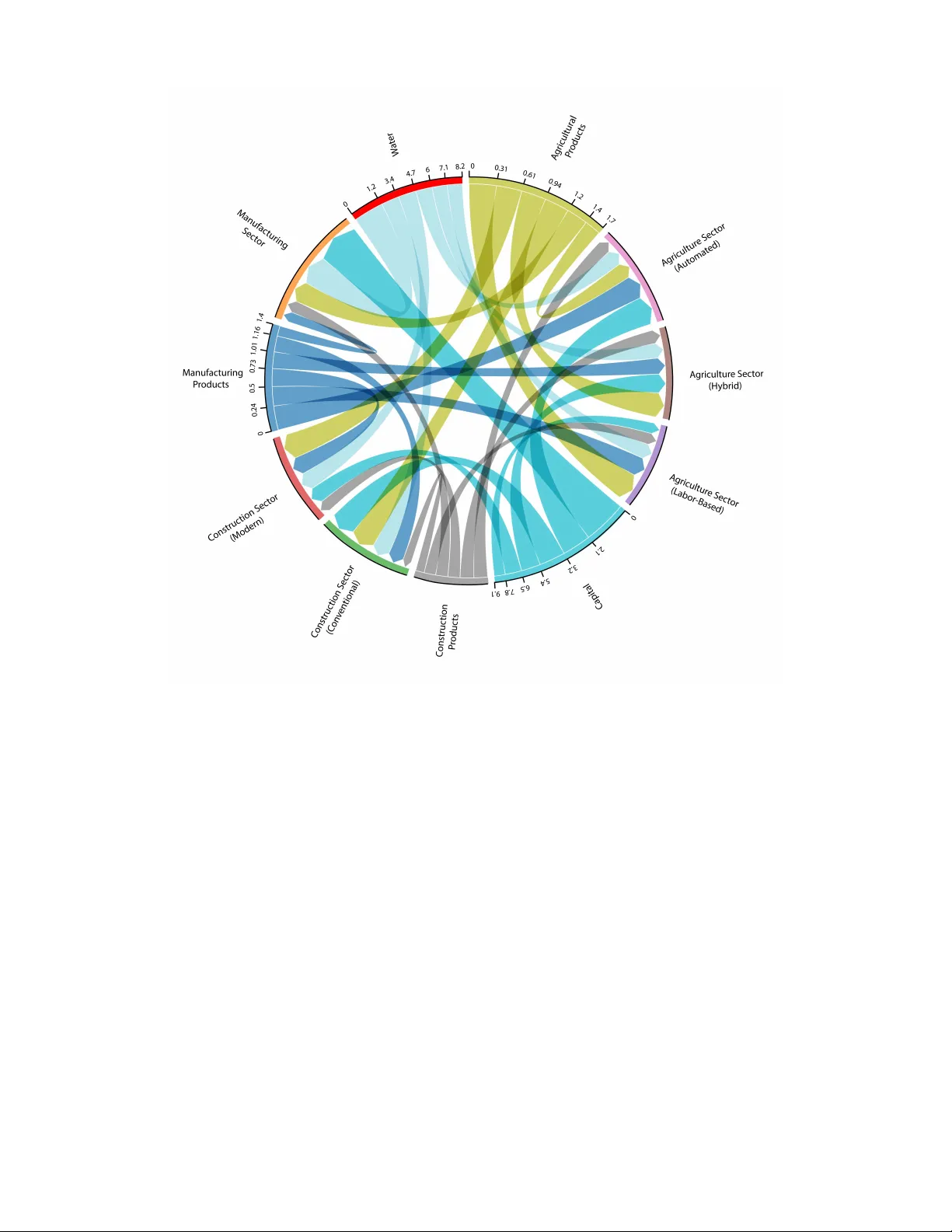
1 Embedding Economic Input–Output Models in Systems of Systems: An MBSE and Hetero-functional Graph Theory Approach Mohammad Mahdi Naderi * 1 , Megan S. Harris 1 , J ohn C. Little 1 , and Amro M. F arid 2 1 Department of Civil and Environmen tal Engineering, Virginia T ech, Blacksburg, Virginia 24061, United Sta tes 2 School of Systems and Enterprises, Stev ens Institute of T echnology , Hoboken, New J ersey , 07030, United Sta tes Abstract Characterizing the interdependent nature of Anthropocene systems of systems is fundamental to making in- formed decisions to address challenges across complex ecological, environmen tal and coupled human-natural systems. This paper presents the ﬁrst application of Model-Based Systems Engineering (MBSE) and Hetero-functional Graph Theory (HFGT) to economic systems, establishing a scalable and extensible methodology for integrating economic input–output (EIO) models within a uniﬁed system-of -systems modeling framework. Integrating EIO models into the MBSE–HFGT workﬂ ow demonstrates how the structural form and function of economic systems can be expressed through SysML ’ s graphical ontology and subsequently translated into the computa tional structure of HFGT . Using a synthetic Rectangular Choice of T echnology (RCOT) example as a pedagogical foundation, the study conﬁrms that the dynamics captured by basic EIO models, as well as other complex economic models grounded in EIO theory , can be equivalentl y reproduced within the MBSE-HFGT framewor k. The integra tion with MBSE and HFGT thus preserves analytical precision while o ﬀ ering enhanced graphical clarity and system-level insight through a shared ontological structure. By integrating modeling languag es and mathematical frameworks, the proposed methodology establishes a foundation for knowledge co-production and integrated decision-making to address the mul tifaceted sustainability challenges associated with Anthropocene systems of systems. I. Introduction Humans are the primary drivers of profound changes in Earth ’ s systems, giving rise to myriad interconnected societal challenges that characterize the Anthropocene [ 1 ]–[ 3 ]. The concept of the Anthropocene describes the current stage of Earth system change in which human activities hav e emerged as a dominant driving force [ 4 ]–[ 8 ], inﬂuencing geophysical, biophysical, socioeconomic, sociocultural, and socio-technical processes [ 1 ]. Rapid popula- tion growth, widespread urbanization, and intensiﬁed resource exploitation are among human-induced pressures [ 9 ] that reshape the Earth ’ s system trajectories and exacerbate intertwined social, ecological, and technological challenges [ 10 ], [ 11 ]. These challenges are inherently interconnected, as disturbances in one system can cascade across the entire system of systems (SoS), generating complex feedback and interactions [ 12 ]–[ 14 ]. For example, rapid economic growth contributes to climate chang e by requiring mass production, destabilizing local hydrological cycles, and changing energy-use regimes [ 15 ], [ 16 ]. The spectrum of Anthropocene challenges is extensive, encompassing global warming, overexpl oitation of natural resources, freshwater scarcity , habitat degradation, and widespread environmental pollution [ 6 ], [ 17 ]. These pressures threaten numerous endangered species and compromise human well-being [ 18 ]. Nonetheless, these challenges are frequently addressed in isolation, with relatively few studies adopting integrativ e approaches that explicitly account for their interdependencies [ 1 ], [ 18 ]–[ 21 ]. Although recent research acknowledges the interconnected nature of Anthropocene challeng es [ 5 ], [ 22 ], [ 23 ], capturing synergies and trade-o ﬀ s across systems remains complicated due to limited understanding [ 24 ], [ 25 ] and the absence of analytical framewor ks capable of quantifying these complex relationships [ 1 ], [ 23 ]. The economic system constitutes a founda tional and inseparable element of the Anthropocene SoS [ 26 ], [ 27 ]. It functions as a primary driver of global change while remaining intrinsically interwoven with and biophysically constrained by social and natural systems [ 28 ], [ 29 ]. This relationship is bidirectional [ 30 ], as the economic system exerts profound impacts on and is signiﬁcantly inﬂuenced by the natural and social spheres, constituting a coupled social–economic–natural SoS [ 31 ], [ 32 ]. One manifesta tion of this is economic growth in the Anthropocene, partic- ularly fossil-fuel-driv en growth, which is responsible for the deterioration of Earth systems and the transgression of planetary boundaries [ 33 ], [ 34 ]. For example, studies indicate that projected biodiversity loss exceeds safe 2 thresholds globally and rises signiﬁcantly with GDP per capita, suggesting that continued economic expansion beyond planetary boundaries undermines the planet ’ s carrying capacity [ 35 ]. In con trast, the economic system is signiﬁcantly inﬂuenced by the other systems through feedback mechanisms [ 2 ], [ 36 ]. For example, resulting environmental changes—such as global warming and extreme events—can suppress economic growth by inducing climate-related damages that compromise water resources, food production, and human health [ 37 ], [ 38 ]. Successfully anticipating the consequences of these interactions between the economic system and other interlinked systems, and e ﬀ ectivel y addressing sustainability challenges, requires models that go beyond traditional approaches, which often treat anthropogenic driv ers as exogenous to the economic system [ 26 ], [ 39 ], [ 40 ]. Consequently , there is a critical need to devel op SoS models that explicitly capture nonlinear , complex dynamics and interdependencies among the economic system and other interconnected systems [ 32 ]. Numerous studies have examined unidirectional and bidirectional causal relationships between the economy and hydrological [ 41 ]–[ 44 ], energy [ 45 ]–[ 48 ], food [ 49 ], and other interconnected systems [ 50 ]–[ 53 ] to assess trade- o ﬀ s and synergies. However , only a limited body of research explicitly conceptualizes the econom y as an integral component of the broader complex SoS in the Anthropocene, in which multidirectional causalities link economic dynamics to other interwoven systems. In most of these studies, this lack of explicit integration is reﬂected in prevailing modeling practices [ 54 ], [ 55 ]. This highlights a predominant reliance on exog enously deﬁned driv ers, constraining the ability to capture the full complexity of cross-system interdependencies. Such limitations arise because modeling approaches for coupling the economic system with other entangled systems often: (i) lack the ca- pacity to represent the full detail of multiple interacting domains, including econom y [ 2 ], (ii) require simpliﬁcation of key elements to reduce complexity [ 56 ], and (iii) face technical and interoperability barriers, as linking distinct models typically demands specialized interfaces [ 23 ]. E ﬀ ective coupling strategies must balance complexity , func- tionality , and computational e ﬃ ciency while sim ultaneously maximizing cross-disciplinary knowledg e integration [ 57 ] through a shared common languag e [ 58 ] and ensuring the internal consistency of the integrated SoS [ 59 ]. A. Objective and Original C ontribution This paper presents the ﬁrst application of Model-Based Systems Engineering (MBSE) and Hetero-functional Graph Theory (HFGT) to economic I-O (EIO) systems, and demonstrates that MBSE-HFGT is well-suited to fully internalize EIO models while capturing the heterogeneous dynamics among economic systems and other interwov en Anthropocene SoS. The paper develops a framewor k for embedding EIO models as key components of complex SoS in the Anthropocene, and demonstrates how these models can be systematically integrated into an MBSE–HFGT workﬂ ow . MBSE provides a formal, ontology -driven environment capable of capturing form, function and heteroge- neous interactions of SoS, enabling all systems—including the economic system—to be represented within a shared common language. The workﬂ ow begins by graphically representing the EIO model in the Systems Modeling Language (SysML) to capture the form and function of the economic system. HFGT is then applied to translate these SysML models into a rigorous computational framewor k. While MBSE can be used as a standalone methodology , this paper shows how coupling MBSE with HFGT provides a powerful quantiﬁcation tool that preserv es the analytical insights of basic EIO models. The MBSE–HFGT framework, therefore, overcomes limitations identiﬁed in prior studies by ensuring ontological consistency between the economic system and other heterogeneous systems, preserving the analytical rigor of EIO models, and extending them to an SoS context as endogenous components, without requiring external interfaces or simplifying assumptions. T o illustra te this integration, the methodology is demonstrated using a synthetic EIO model commonly used in the literature by modelers across disciplines to eval uate sectoral economic dynamics. This example conﬁrms that MBSE–HFGT not only can reproduce the analytical insights of economic modeling within an integrated SoS platform but also o ﬀ ers greater graphical clarity and system-level insight through a shared ontol ogy that facilitates the co-production of knowledge and cross-disciplinary understanding. In doing so, the paper bridges a critical gap between economic modeling and systems engineering, establishing a uniﬁed ontological and mathematical foundation for integra ted decision-making in complex socio-economic–environmental Anthropocene SoS. B. Paper Outline The remainder of the paper is organized as follows. Sec. II- A introduces the fundamentals of EIO models. Sec. II-B elaborates on MBSE and graphical models of system form and function in SysML. Sec. II-C presents essential background on HFGT , and Sec. III provides a synthetic, motivational RCOT example and demonstrates how MBSE- HFGT can be applied to internalize it. Sec. IV discusses the implications of these results for simulating EIO models and for addressing societal challenges that cascade through interconnected systems. Sec. V brings the paper to a conclusion. 3 II. Conceptual and Theoretical B ackground A. Economic Input–Output (EIO) Model EIO modeling, originally developed by Leontief (1936) [ 60 ], captures the interdependencies of production and consumption within an economic system [ 61 ]. Over time, EIO models have been increasingly utilized in eco- nomic–environmental analyses to eval uate environmental sustainability [ 62 ]–[ 64 ], energy management [ 65 ], [ 66 ], risk assessment [ 67 ], [ 68 ], and complex nexus systems [ 69 ]–[ 71 ]. EIO models evaluate direct, indirect , and ind uced impacts, which together provide a more comprehensive view of the dynamics of an economic system [ 72 ], [ 73 ]. The scientiﬁc literature identiﬁes three main types of EIO models: basic (monetary) EIO, physical EIO, and hybrid EIO models [ 61 ]. The basic EIO model accounts for intersectoral ﬂows in monetary units (e.g., euros), the physical EIO model in physical units (e.g., tons), and the hybrid EIO model in a mixed-unit framework, combining monetary and ph ysical units as needed [ 61 ], [ 74 ]–[ 76 ]. These models share the common foundation of EIO accounting, which captures the balance between the supply and use of products across sectors. EIO models are based on the product supply–use equilibrium published in EIO tables. The equilibrium can be expressed as: x = Z 1 + y (1) where x is a column vector of economic output with n rows corresponding to industries, Z is an n × n matrix of intermediate sales, y is a column vector of ﬁnal demand with n rows, and 1 is a column vector of ones. The technical coe ﬃ cients matrix A represents the share of goods and services required for production. Its elements a i j = z i j / x j where z i j denotes the quantity of intermediate goods i sold by industry j , and x j represents the total economic output of industry j . The model assumes that the matrix of technical coe ﬃ cients is constant , reﬂecting the model’ s linearity . Finally , Eq. 2 is obtained by substituting the technical coe ﬃ cients matrix A into Eq. 1 and performing factorization. x = ( I − A ) − 1 y = By (2) where B = ( I − A ) − 1 is the Leontief inv erse matrix. Its elements b i j quantify the total, direct and indirect, e ﬀ ect on the output of industry j due to a one-unit change in ﬁnal demand for product i . Additionally , to compute the factor use vector φ , the ﬁnal output vector x is multiplied by the factor requirement matrix F : φ = F x (3) Building on this foundation, basic EIO modeling can be extended to economic input -output life-cycle assessment (EIO-L C A) [ 77 ], [ 78 ], multi-region input–output (MRIO) [ 79 ], [ 80 ], rectangular choice of technology (RCOT) [ 81 ], [ 82 ], environmentall y-extended input -output (EEIO) [ 83 ]–[ 85 ] and ecologically -extended input -output (ECEIO) [ 86 ], among others. The RCOT model, as an extension of the basic EIO formulation, endows each sector with the capacity to select among multiple alternative technologies [ 82 ], [ 87 ], [ 88 ]. T o do this, the basic EIO model can be reformulated to accommodate alternativ e technologies by expanding the matrices I, A, and F with additional columns representing these technological options, thereby inducing a corresponding augmentation of the ﬁnal output vector , x [ 81 ]. T o demonstrate this, each sector i can choose from among T alternativ e technologies. The resulting model can be expressed accordingly as a generalization of Eq. 2 : ( I ∗ − A ∗ ) x ∗ ≥ y (4) f ≤ F ∗ x ∗ , (5) where x ∗ is a T × 1 vector , I ∗ and A ∗ are n × t matrices, y remains n × 1, F ∗ is a k × t matrix, and f remains k × 1. In general, k increases relative to the basic model if some technology -speciﬁc factors are included for the new options. The objective is formulated as the minimization of total factor use. Individual factors are weighted in accordance with their respective prices, represented by the inner product π ′ f . The resulting optimization problem can therefore be expressed as a linear program of the form: min Z = π ′ F ∗ x ∗ (6a) subject to ( I ∗ − A ∗ ) x ∗ ≥ y (6b) In this formulation: • I ∗ ( n × t ) denotes an incidence matrix, representing each sector’ s self -requirements across all alternative tech- nologies. • A ∗ ( n × t ) is the augmented inter -industry transaction matrix, capturing the input requirements of each sector for every technology choice. • x ∗ ( t × 1) is the vector of total outputs associated with each technology option. 4 • y ( t × 1) represents the ﬁnal demand, remaining unchanged from the basic EIO model. • F ∗ ( k × t ) speciﬁes factor requirement per unit of output. • π ( k × 1) is the v ector of factor prices used to weight these intensities in the objective function. • and f ( k × 1) is the factor availability vector . T ogether , these augmented matrices and vectors allow the RC OT model to systematically represent both sectoral interdependencies and technology-speciﬁc factor requirements, enabling the optimization of total factor use while accounting for alternativ e technological options. B. Model-Based Systems Engineering (MBSE) In systems engineering, models serve as indispensable tools for understanding complex systems, enabling experi- ments, operations, and stakeholder negotiations by representing key aspects of the world from a speciﬁc perspective while simplifying it through abstractions that omit irrelevant details [ 89 ]–[ 91 ]. MBSE builds on this foundation as a standard, ﬂexible modeling approach that uses a broad set of abstractions for the design and analysis of complex systems, including economic systems [ 59 ], [ 92 ]. Rather than treating economic, hydrologic, social, and other interlinked systems as isolated entities, MBSE provides a uniﬁed framework that integrates these domains, capturing both form (the physical or logical elements) and function (the processes that transform inputs into outputs) within a common modeling languag e [ 93 ], [ 94 ]. In the context of economic modeling, MBSE act as a bridge between historically fragmen ted modeling approaches. For example, while economic models estimate changes in supply and demand, MBSE can facilitate their integration with land-use, hydrol ogic, ecosystem, energy , and other interconnected systems [ 95 ]. This holistic perspective enables detailed graphical representations and simulations of economic processes within a common ontological framewor k and provides insight into their interactions within a larger SoS. SysML provides a standardized set of diagrams for representing system architecture within MBSE. SysML diagrams exhibit three broad categories of systems thinking abstractions to graphically describe a system: 1) system boundary , 2) system form, and 3) system function. This generic pattern constitutes a reference architecture (RA) [ 96 ], which can signiﬁcantly reduce the cognitive complexity associated with understanding these systems. Among the SysML diagrams, the Block Deﬁnition Diagram (BDD) captures the system form by specifying the hierarch y of its structural elements, their constituents and attributes, and how they are connected and/or related. In economic systems, these might represent physical elements like industrial sectors and production facilities. Relationships among these physical elements can be represented by a broad set of interconnection abstractions, such as encapsulation, decomposition, ag gregation, g eneralization, and classiﬁcation [ 59 ], [ 97 ]. Instan tiation relationships are also important, as they describe connections at a generic level rather than specifying them for each and every instance [ 98 ]. For example, in economic systems, the agricultural sector generall y sells its products to speciﬁc industrial sectors. Similarly , the Activity Diagram (A CT) describes what a system does and how it behav es [ 97 ], [ 99 ]. A CT diagrams explicitly illustra te the ﬂow of processes showing how activities transform inputs into outputs. For example, the transfer of energy from its source to the sectors that consume it to genera te speciﬁc industrial products [ 100 ], [ 101 ]. In A CT diagrams, no restrictions are imposed on the type of system state; for instance, Lagrangian, power , and Hamiltonian variables ma y be deﬁned over real numbers, complex n umbers, integ ers, or even booleans. Moreover , continuous- time, discrete-time, discrete-event, and hybrid state evolutions can be straightforwardly simulated within A CT diagrams. These capabilities enable modelers to capture details of economic systems with enhanced accuracy , thereby reducing uncertainty and facilitating more rigorous analyses of complex interdependencies and dynamic beha viors. It should be noted that functional interactions in A CT and formal interfaces (i.e., associations) in BDD are equivalent only when the allocation of function to form is one-to-one [ 96 ], [ 99 ]. In BDD and A CT diagrams, the system boundary delineates between the system itself and everything else (in the system context) [ 96 ]. In SysML, the system boundary is alwa ys explicitly depicted by the diagram boundary , regardless of the diagram type. This boundary is labeled in the top left corner of each diagram with four pieces of information, presented in order: 1) the type of diagram (e.g., BDD, A CT), 2) the type of model element (e.g., block, activity), 3) the name of the model element, and 4) the name of the diagram [ 59 ], [ 97 ]. Whether a system boundary is open or closed is made explicit in SysML. If a block in BDD has a connecting arrow , it is considered an open system in its own right. Likewise, any activity in A CT with a connecting arrow is treated as an open system activity . In contrast, the lack of connecting arrows signiﬁes a closed system. Explicitly deﬁning the system boundary allows economic modelers to clearly distinguish between endogenous and exogenous factors, improving model structure, interpretation, and the reliability of scenario analyses. Ultimatel y , SysML diagrams enhance shared understanding and support the co-production of knowledge when practitioners from diverse disciplines—including economics, hydrol ogy , energy , and land use—conduct modeling within a common ontology [ 102 ]. This interdisciplinary coherence contributes to a modeling process that is more legitimate, credible, and salient [ 103 ], [ 104 ]. 5 C. Hetero-Functional Graph Theory (HFGT) While MBSE, and speciﬁcally SysML, o ﬀ ers a uniﬁed modeling language [ 1 ] for complex SoS, it inherently lacks the tools necessary for robust, larg e-scale quantitativ e analyses. Fortunately , HFGT [ 105 ]–[ 107 ] provides an analytical framewor k for converting graphical SysML representations into formal mathematical and computational models. HFGT has been applied to single-domain systems such as electric power [ 108 ], [ 109 ], potable water [ 110 ], transportation [ 111 ], and mass-customized production systems [ 112 ]–[ 115 ]. Its applica tion extends to SoS, including mul ti-modal electriﬁed transportation [ 116 ]–[ 118 ], microgrid-enabled production systems [ 119 ], hydrol ogic mod- eling [ 120 ], personalized healthcare delivery [ 121 ]–[ 123 ], hydrog en-natural gas systems [ 124 ], the energy-wa ter nexus [ 125 ], and the American multi-modal energy system [ 126 ]. Notably , several of these SoS applications of HFGT integrate both time-driv en and discrete-event dynamics. Additionally , recent studies have shown that MBSE-HFGT can formall y generalize and extend process-based life- cycle assessment (LC A) [ 127 ], [ 128 ], whose conceptual founda tions closel y align with EIO systems. These studies hav e reconciled LC A with the shared language of MBSE-HFGT and have demonstrated that MBSE-HFGT is a formal generaliza tion of process-based LC A. They also show how MBSE-HFGT can enhance the spatio-tem poral resol ution of L CA to align it with system design objectiv es [ 127 ] and adopt dynamic, data-driv en approaches—such as real-time carbon intensity , operational adaptation, and cost ﬂuctuations—to more accuratel y quantify environmental burdens. T ogether , these advances reﬂect the same underlying principles that support other extensions of EIO models—such as MRIO, EEIO, and ECEIO—which capture spatio-temporal dynamics of interdependent ﬂows [ 129 ] to characterize system-wide sustainability outcomes. 1) Essential Deﬁnitions: Hetero-functional graphs (HFGs) are f ormal graphical models that represent the in tercon- nectedness of complex SoS. HFGT is conceptually rooted in the universal structural principles of human languag e, particularly subjects and predicates, where predicates consist of verbs and objects [ 105 ], [ 106 ]. This reliance on the structure of human language provides the basis for a discipline-agnostic ontology that facilitates cross-disciplinary applications [ 58 ]. In HFGT , a system is deﬁned by a set of resources R , which act as the subjects; a set of processes P , which serve as predicates; and a set of operands L , which constitute the objects involv ed in these processes. Deﬁnition 1 – System Operand [ 130 ]: An asset or object l i ∈ L that is operated on or utilized in the course of a process execution. ■ Deﬁnition 2 – System Process [ 130 ], [ 131 ]: An activity p ∈ P that converts or transf ers a speciﬁed set of input operands into a designated set of outputs. ■ Deﬁnition 3 – System Resource [ 130 ]: An asset or object r v ∈ R that enables the execution of a process. ■ The system resources R = M ∪ B ∪ H are categorized into transformation resources M , independent bu ﬀ ers B , and transportation resources H . The set of “bu ﬀ ers” B S = M ∪ B is introduced to support the discussion, and the system processes P = P µ ∪ P ¯ η are classiﬁed into transf ormation processes P µ and reﬁned transportation processes P η . This occurs from the concurrent execution of a transportation process and a holding process. HFGT further highlights that resources can perform one or more system processes, thereby genera ting a set of “capabilities” [ 105 ]. Deﬁnition 4 – Bu ﬀ er [ 105 ], [ 106 ]: A resource r v ∈ R is a bu ﬀ er b s ∈ B S if and only if it has the capacity to store or transform one or more operands at a speciﬁc spatial location. ■ Deﬁnition 5 – Capability [ 105 ]–[ 107 ]: An action e wv ∈ E S (in the SysML sense) deﬁned by a system process p w ∈ P being executed by a resource r v ∈ R . It constitutes a subject + verb + operand sentence of the form: “Resource r v does process p w ” . ■ In HFGT , the engineering system meta- architecture must be instantiated and eventually translated into corre- sponding P etri net model(s) [ 106 ]. T o facilitate this, the positive and negativ e hetero-functional incidence tensors are introduced to characterize the ﬂow of operands through bu ﬀ ers and capabilities. Deﬁnition 6 – The Negative 3 r d Order Hetero-functional Incidence T ensor (HFIT f M − ρ [ 106 ]): The negative hetero-functional incidence tensor g M ρ − ∈ { 0 , 1 } | L |×| B S |×|E S | is a third-order tensor whose element f M − ρ ( i , y , ψ ) = 1 when the system capability ϵ ψ ∈ E S pulls operand l i ∈ L from bu ﬀ er b s y ∈ B S . ■ Deﬁnition 7 – The P ositive 3 r d Order Hetero-functional Incidence T ensor (HFIT f M + ρ [ 106 ]): The positive hetero-functional incidence tensor f M + ρ ∈ { 0 , 1 } | L |×| B S |×|E S | is a third-order tensor whose element f M + ρ ( i , y , ψ ) = 1 when the system capability ϵ ψ ∈ E S injects operand l i ∈ L into bu ﬀ er b s y ∈ B S . ■ These incidence tensors are straightforwardly “matricized” to form second-order Hetero-functional Incidence Ma- trices M = M + − M − with dimensions | L || B S | × |E | . Consequently , the supply , demand, transportation, storage, trans- formation, assembly , and disassembly of multiple operands in distinct loca tions over time can be described by an Engineering System Net and its associated State T ransition Function [ 124 ]. 6 Deﬁnition 8 – Engineering System Net [ 124 ]: An elementary P etri net N = { S , E S , M , W , Q } , where: • S is the set of places with size: | L || B S | , • E S is the set of transitions with size: |E | , • M is the set of arcs, with the associated incidence matrices: M = M + − M − , • W is the set of w eights on the arcs, as captured in the incidence matrices, • Q = [ Q B ; Q E ] is the marking vector for both the set of places and the set of transitions. ■ Deﬁnition 9 – Engineering System Net State T ransition Function [ 124 ]: The state transition function of the engineering system net Φ () is: Q [ k + 1] = Φ ( Q [ k ] , U − [ k ] , U + [ k ]) ∀ k ∈ { 1 , . . . , K } (7) where k is the discrete time index, K is the simulation horizon, Q = [ Q B ; Q E ], Q B has size | L || B S | × 1, Q E has size |E S | × 1, the input ﬁring vector U − [ k ] has size |E S | × 1, and the output ﬁring v ector U + [ k ] has size |E S | × 1. Q B [ k + 1] = Q B [ k ] + M + U + [ k ] ∆ T − M − U − [ k ] ∆ T (8a) Q E [ k + 1] = Q E [ k ] − U + [ k ] ∆ T + U − [ k ] ∆ T (8b) where ∆ T is the duration of the simulation time step. ■ It is crucial to mention that the engineering system net’ s state transition function explicitly embodies continuity laws, allowing both the Eulerian and Lagrangian perspectiv es depending on the required modeling application. In addition to the engineering system net, each operand in HFGT can hav e its own state and evolution. This behavior is described by an Operand Net and its associated S tate T ransition Function for each operand. Deﬁnition 10 – Operand Net [ 105 ], [ 114 ], [ 119 ], [ 122 ]: Given operand l i , an elementary P etri net N l i = { S l i , E l i , M l i , W l i , Q l i } where: • S l i is the set of places describing the operand’ s state. • E l i is the set of transitions describing the evol ution of the operand’ s state. • M l i ⊆ ( S l i × E l i ) ∪ ( E l i × S l i ) is the set of arcs, with the associated incidence matrices: M l i = M + l i − M − l i ∀ l i ∈ L . • W l i : M l i is the set of weights on the arcs, as captured in the incidence matrices M + l i , M − l i ∀ l i ∈ L . • Q l i = [ Q S l i ; Q E l i ] is the marking vector for both the set of places and the set of transitions. ■ Deﬁnition 11 – Operand Net Sta te T ransition Function [ 105 ], [ 114 ], [ 119 ], [ 122 ]: The state transition function of each operand net Φ l i () is: Q l i [ k + 1] = Φ l i ( Q l i [ k ] , U − l i [ k ] , U + l i [ k ]) ∀ k ∈ { 1 , . . . , K } i ∈ { 1 , . . . , L } (9) where Q l i = [ Q S l i ; Q E l i ], Q S l i has size | S l i | × 1, Q E l i has size |E l i | × 1, the input ﬁring vector U − l i [ k ] has size |E l i | × 1, and the output ﬁring vector U + [ k ] has size |E l i | × 1. Q S l i [ k + 1] = Q S l i [ k ] + M l i + U + l i [ k ] ∆ T − M l i − U − l i [ k ] ∆ T (10a) Q E l i [ k + 1] = Q E l i [ k ] − U + l i [ k ] ∆ T + U − l i [ k ] ∆ T (10b) ■ 2) The Hetero-functional Network Minimum Cost Flow (HFNMCF) Problem: HFGT simulates the behavior of an engineering system using the Hetero-Functional Network Minimum Cost Flow (HFNMCF) problem [ 124 ]. The HFNMCF problem extends the classical network minimum-cost ﬂow problem to account for the heterogeneity of functions observed in Anthropocene SoS. It optimizes the time-dependent ﬂow and storage of mul tiple operands among bu ﬀ ers, enables transformation from one operand to another , and tracks the state of these operands. In this regard, it is a highly ﬂexible optimization problem applicable to a wide range of complex engineering systems. For the purposes of this paper , the HFNMCF problem is a type of discrete-time-dependent, time-inv ariant , convex optimization program [ 124 ]. Z = K − 1 X k =1 x T [ k ] F QP x [ k ] + f T QP x [ k ] (11a) s.t. − Q B [ k + 1] + Q B [ k ] + M + U + [ k ] ∆ T − M − U − [ k ] ∆ T =0 ∀ k ∈ { 1 , . . . , K } (11b) 7 − Q E [ k + 1] + Q E [ k ] − U + [ k ] ∆ T + U − [ k ] ∆ T =0 ∀ k ∈ { 1 , . . . , K } (11c) − U + ψ [ k + k d ψ ] + U − ψ [ k ] =0 ∀ k ∈ { 1 , . . . , K } ψ ∈ { 1 , . . . , E S } (11d) − Q S l i [ k + 1] + Q S l i [ k ] + M + l i U + l i [ k ] ∆ T − M − l i U − l i [ k ] ∆ T =0 ∀ k ∈ { 1 , . . . , K } i ∈ { 1 , . . . , | L |} (11e) − Q E l i [ k + 1] + Q E l i [ k ] − U + l i [ k ] ∆ T + U − l i [ k ] ∆ T =0 ∀ k ∈ { 1 , . . . , K } i ∈ { 1 , . . . , | L |} (11f) − U + xl i [ k + k d xl i ] + U − xl i [ k ] =0 ∀ k ∈ { 1 , . . . , K } , ∀ x ∈ { 1 , . . . , |E l i }| , l i ∈ { 1 , . . . , | L |} (11g) U + L [ k ] − b Λ + U + [ k ] =0 ∀ k ∈ { 1 , . . . , K } (11h) U − L [ k ] − b Λ − U − [ k ] =0 ∀ k ∈ { 1 , . . . , K } (11i) " D U p 0 0 D U n # " U + U − # [ k ] = " C U p C U n # [ k ] ∀ k ∈ { 1 , . . . , K } (11j) " E Lp 0 0 E Ln # " U + l i U − l i # [ k ] = " F Lpi F Lni # [ k ] ∀ k ∈ { 1 , . . . , K } i ∈ { 1 , . . . , | L |} (11k) h Q B ; Q E ; Q S L i [1] = h C B 1 ; C E 1 ; C S L 1 i (11l) h Q B ; Q E ; Q S L ; U − ; U − L i [ K + 1] = h C BK ; C E K ; C S LK ; 0 ; 0 i (11m) E C P ≤ D ( X ) ≤ E C P (11n) g ( X , Y ) =0 (11o) h ( Y ) ≤ 0 (11p) where X = [ x [1]; . . . ; x [ K ] ] is the v ector of primary decision variables, and Y = [ y [1]; . . . ; y [ K ] ] is the v ector of auxiliary decision variables at time k . III. A Motiv ational Example: Appl ying MBSE-HFGT to an EIO model T o support the remainder of the paper’ s contribution, this section introduces a motiv ational example to compare and contrast EIO models with MBSE and HFGT . Subsection III- A describes the RCOT model example. Subsection III-B presents the dev elopment of the economic system RA under the HFGT meta- architecture to represent the form and the function of the RCOT example. F inally , Subsection III-C derives a system of equations in accordance with the HFNMCF problem outlined in Subsection II-C2 to quantitatively show how MBSE-HFGT reproduces the same results as the traditional RCOT model. This provides an instructive foundation, illustrating the methodology in a scenario that is both tractable and conceptually rich. A. Economic Input Output (EIO) Model This section describes an example economic system using the Rectangular Choice of T echnology (RCOT) model described by Duchin [ 81 ]. The synthetic economy example is illustr ated in Fig 1 . It is speciﬁed by the following matrices and vectors that constitute the RCOT formulation. I ∗ =         1 0 0 0 0 0 0 1 1 0 0 0 0 0 0 1 1 1         3 × 6 , A ∗ =         0 . 35 0 . 15 0 . 23 0 . 26 0 . 28 0 . 24 0 . 25 0 . 22 0 . 16 0 . 22 0 . 21 0 . 25 0 . 20 0 . 26 0 . 30 0 . 31 0 . 33 0 . 30         3 × 6 F ∗ = " 2 . 1 3 . 2 1 . 9 1 . 2 0 . 8 1 . 4 1 . 2 2 . 2 1 . 3 1 . 3 1 . 1 1 . 1 # 2 × 6 , y =         20 25 22         3 × 1 , f = " 540 342 # 2 × 1 , π = " 1 0 . 9 # 2 × 1 . As quantiﬁed in the matrices above, the economic system comprises n = 3 sectors and k = 2 primary factors of production. The sectors di ﬀ er in the number of technological alternativ es available to them. For clarity , technolog- ical options are conventionally assigned to the foll owing sectors. Sector 1 (manuf acturing) is limited to a single technology ( t 1 = 1). Sector 2 (construction) has access to two al ternative technologies ( t 2 = 2). Sector 3 (agriculture) can operate with three technological options ( t 3 = 3). This conﬁguration yields a total of T = 6 distinct technologies for the economy as a whole. The factors of production are restricted to two essential inputs: water and capital. T ogether , they span the system ’ s resource requirements. 8 Fig. 1: Inter -industrial relationships of economic sectors in terms of technical coe ﬃ cients Solving the RCOT optimization problem yields the optimal value Z, the ﬁnal output vector , x , and the corre- sponding factor use vector , φ . Z = 805 . 724 , x =                      99 . 7883 0 87 . 5364 0 26 . 6400 71 . 9500                      6 × 1 , φ = " 498 . 92 342 . 00 # 2 × 1 . B. Model-Based Systems Engineering (MBSE) Next, the EIO example introduced in the previous subsection is modeled as a SysML RA (as described previously in Sec. II-B ). By situating the EIO model within a SysML RA, the form and function of the economic system ’ s architecture is elucidated. T o that end, a domain-speciﬁc economic system RA is dev eloped as a special case of the (domain-independent) HFGT meta-architecture. Fig. 2 shows the form of the economic system as a BDD. Importantly , core HFGT concepts — such as resources, processes, and operands — are mapped to their counterparts in the EIO model. Fig. 3 shows the function of the economic system as an A CT . It graphically depicts intersectoral transactions, factor -use allocations, and ﬁnal-demand ﬂows. It is important to recognize that the reference architec- ture of the economic system can be readily extended, either within the A CT by adding new functions (e.g., economic activities) or within the BDD by incorporating new regional economies or entirely di ﬀ erent (non-economic) systems. C. Hetero-functional Graph Theory (HFGT) The domain-independent HFGT deﬁnitions introduced in Section II-C acquire domain-speciﬁc signiﬁcance in the context of the EIO system model introduced in Sec. III- A . More speciﬁcally , the system operands L (Def . 1 ) 9 are water , capital, and the outputs from the manufacturing, construction, and agricultural sectors. The system processes P (Def. 2 ) appear as the six operations in “The Economy” block in Fig. 2 . Collectively , they correspond to the economic mechanisms responsible for the production of agricultural, manufacturing, and construction products. The system resources R (Def . 3 ) carry out the system processes. In the context of the EIO model, the whole econom y is a transformation resource ( M ) that realizes all the processes. Because the EIO model focuses on functions, their inputs, and their outputs, there are no other system resources. The capabilities E S (Def. 5 ) combined the resources and processes into subject + predicate sentences. For example, the economy produces agricul tural products with automated technologies. Fig. 2: Block Deﬁnition Diagram that deﬁnes the EIO model form. T o internalize the objective function and the constraint of the RCOT model (i.e., Eqs. 4 and 5 ) within HFGT , we reformula te them as the following equation:  I ∗ − A ∗ − F  x ≥  y − f  (12) The right -hand side represents a vertically concatenated vector composed of the ﬁnal demand ( y ) and factor av ailability ( f ), giv en by: " y − f # =                 Manuf acturing products Construction products Agricultur al products Capital W ater                 (13) The ﬁnal output vector x is also expressed as: x =                      Economy produces manufactured products Economy produces construction products with conventional technology Economy produces construction products with modern technology Economy produces agricultural products with labor -based technology Economy produces agricultural products with hybrid technology Economy produces agricultural products with automated technology                      (14) Each element of the vector x represents a distinct capability associated with the economic system, characterizing a speciﬁc process undertaken to produce inter -industry outputs (see Fig. 2 and 3 ). In other words, each entry in this vector adheres to the “Subject + V erb + Object” construct of the HFGT framework described in Sec. II-C . The conﬁguration of the engineering system net, represented by Q B , is designed to capture the heterog eneity of system bu ﬀ ers and operands. Accordingly , Q B is organized as a composite structure consisting of ﬁve vertically concatenated v ectors: 10 Fig. 3: Activity Diagram that deﬁnes the EIO model function. Q B = h Q Economy -ManProd , Q Economy -ConsProd , Q Economy - AgProd , Q Economy - W ater , Q Economy -Capital i (15) The notation Q Economy is introduced to represent the ﬁve elements of Q B corresponding to the set of ﬁve operands, expressed in million-dollar units except for wa ter , which is giv en in million-gallon units. Subsequently , the tran- sitions of the engineering system network, U , are structured to capture the distinct capabilities of the economic system. Accordingly , U is organized as a composite entity comprising six vertically concatenated vectors. U = h U ProduceManProd , U ProduseConsProd-ConvT ech , U ProduseConsProd-ModT ech , U ProduceAgProd-LaborT ech , U ProduceAgProd-HybridT ech , U ProduceAgProd- AutoT ech i Owing to the inherent structural regularities and simplifying characteristics of the EIO model, the general formula tion of the HFNMCF optimization problem presented in Eqs. 11a to 11p reduces to the following specialized form: minimize Z = π ′ F ∗ U (16) M U ≥ C (17) • The objective function in Eq. 11a simpliﬁes to Eq. 16 , conveying the same formula tion, with the distinction that , as discussed above, x = U in this instance. • Eq. 11b simpliﬁes to Eq. 17 , where C =  y − f  represents the vector encompassing all operands within the economic system. The equality constraint in Eq. 11b was reformula ted as the inequality in Eq. 17 because the basic EIO formulation omits the marking vector Q at both the current and future time steps. In e ﬀ ect , if the inequality in the EIO model 11 were conv erted into an equality with its associated surplus variable [ 132 ]–[ 134 ], it would represent the surplus found in the marking vector Q . The elimination of storage in a surplus variable removes the need for temporal modeling in the EIO model. The original rationale for using an inequality in EIO formula tions is not clearly documented. Howev er , this paper h ypothesizes that this relaxation was introduced to accommodate empirical data limitations. Historically , EIO tables were compiled from surveys and self -reported statistics, which often contained measurement errors, rounding inconsistencies, or incomplete entries. By expressing ﬂow balances as inequalities rather than strict equalities, modelers could obtain feasible solutions even when the reported data violated perfect conserva tion, thereby tolerating uncertainty and structural inconsistencies [ 135 ]. T o demonstrate the methodology introduced in III , this section instantiates a canonical EIO conﬁguration, de- scribed in Subsection III- A . T o decipher the mechanism of the engineering system net incidence matrix, the system is ﬁrst represented as a colored P etri net in Fig 4 . This P etri net is the instantiated version of the example system described in Subsection III- A within the economic system RA (Sec. III-B ) which captures the dynamics of operands (i.e. both factors of production and inter -industry products) as they ﬂow through the economic system. In the P etri net, operands are contained within discrete places (circles). W ater (blue), capital (gray), agricultural products (green), man ufacturing products (brown), and construction prod ucts (or ange) are represented as tokens that undergo transformation processes through transitions—equivalent to the system ’ s capabilities—which encode the production and exchange mechanisms gov erning the ﬂow of operands within the system. Fig. 4: Colored P etri Net representation of the EIO model The P etri net, along with its underlying architectural schema, is encoded in an XML ﬁle and processed using the HFGT toolbox [ 136 ]. This toolbox generates the hetero-functional incidence tensors and their associated metadata in JSON format. Therefore, the engineering system net incidence matrix takes a block matrix form: M + =                 1 0 0 0 0 0 0 1 1 0 0 0 0 0 0 1 1 1 0 0 0 0 0 0 0 0 0 0 0 0                 , M − =                 0 . 35 0 . 15 0 . 23 0 . 26 0 . 28 0 . 24 0 . 25 0 . 22 0 . 16 0 . 22 0 . 21 0 . 25 0 . 20 0 . 26 0 . 30 0 . 31 0 . 33 0 . 30 2 . 1 3 . 2 1 . 9 1 . 2 0 . 8 1 . 4 1 . 2 2 . 2 1 . 3 1 . 3 1 . 1 1 . 1                 , M = M + − M − =                 0 . 65 − 0 . 15 − 0 . 23 − 0 . 26 − 0 . 28 − 0 . 24 − 0 . 25 0 . 78 0 . 84 − 0 . 16 − 0 . 22 − 0 . 25 − 0 . 20 − 0 . 26 − 0 . 30 0 . 69 0 . 67 0 . 70 − 2 . 1 − 3 . 2 − 1 . 9 − 1 . 2 − 0 . 8 − 1 . 4 − 1 . 2 − 2 . 2 − 1 . 3 − 1 . 3 − 1 . 1 − 1 . 1                 The JSON output from the HFGT toolbox is then imported into a Julia-based simulation environment where the HFNMCF problem is solved. The simulation results for the synthetic EIO model show complete agreement between 12 the RCOT model and the HFNMCF problem (T able I ). The solution of the HFNMCF problem demonstrates how the MBSE-HFGT framework can capture the dynamics of an RCOT model. More importantly , these results indicate that the RCOT model can be regarded as a special case of the MBSE-HFGT framework, suggesting that more complex versions of the EIO model—such as MRIO and EEIO—can also be represented within the MBSE-HFGT framework. T ABLE I: Optimized val ues for capabilities ( U ) (i.e., ﬁnal output ( x ) in RC OT), objective v alue ( Z ), and f actor use ( φ ∗ ). Capability V alue P ercentage of total Economy produces manufactured products 99.7883 33.0% Economy produces construction products with conventional technology 0.0000 0.0% Economy produces construction products with modern technology 87.5364 29.0% Economy produces agricultural products with labor -based technology 0.0000 0.0% Economy produces agricultural products with hybrid technology 26.6439 8.8% Economy produces agricultural products with automated technology 71.9531 23.8% T otal 286 Objective Z 805.7241 F actor use φ ∗ Capital 498.92 (Million $) W ater 342.00 (Million gallons) IV . Discussion Internalizing EIO models within the MBSE–HFGT framework demonstrates the scalability , extensibility , and integrativ e capacity of this framewor k for modeling economic systems. The RC OT synthetic example serv ed as a pedagogical foundation, conﬁrming that modeling multi-domain economic systems with detailed representation of heterogeneous system entities, variables, interdependencies, and structural dynamics can be addressed using the broad set of abstractions and a common language in SysML ’ s rich graphical ontology . MBSE expressed in SysML provides a n uanced means of deﬁning system boundaries, form, and function, while capturing the inherent nature of diverse entities and their interdependencies within EIO models. A key novelty of this wor k lies in the graphical representation of the economic system ’ s structural form and function within SysML, presented here for the ﬁrst time. Moreover , the RCOT example conﬁrms that the core inter -industrial dynamics of an EIO model can be represented through the uniﬁed mathematical structure of HFGT , reproducing results equivalent to those obtained from the standard EIO approach. Extending the approach to other economic models with considerabl y greater complexity that are rooted in EIO fundamentals should be achievable through the framewor k’ s extensibility . In such cases, system-speciﬁc tensors are a utomatically generated via the HFGT toolbox, enabling more complex dynamics to be incorporated without altering the underlying ontology . T ogether , these results highlight the broader val ue of MBSE–HFGT in supporting the simulation of complex, heterogeneous EIO systems. Such heterogeneity includes algebraic, di ﬀ erential, and di ﬀ erential- algebraic equations, whether linear or nonlinear , as well as deterministic and stochastic models with continuous and discrete variables. In this uniﬁed modeling framework, the many features of SysML and HFGT provide an e ﬀ ective computational approach capable of handling the diverse characteristics of Anthropocene SoS, including economic systems. Rep- resenting all models within a common ontology also enables knowledge co-production, o ﬀ ering a pathway to address the complex challenges of contemporary sustainability more e ﬀ ectiv ely than traditional approaches [ 137 ], [ 138 ]. Applying this comprehensive approach aligns with the National Science Foundation ’ s Growing Converg ence Research (GCR) initiative, which aims for deep integration across disciplines to address pressing societal challenges [ 139 ]. V . Conclusion and future work T o integrativ ely address the interdependent societal challeng es of the An thropocene, an SoS con vergence paradigm that includes a computational framework, decision-support system, and educational pedagogy is required [ 1 ]. Howev er , the v ast number of interacting systems and the heterogeneity of their discipline-speciﬁc ontologies make the direct integration of their models practically infeasible. The MBSE–HFGT framework provides researchers and practitioners across diverse domains—such as hydrology , land use, economics, energy , and healthcare—with a pragmatic and systematic tool for integrativel y modeling and addressing complex problems that propagate across interconnected systems with a uniﬁed modeling languag e. This study presents the ﬁrst application of the MBSE–HFGT framework to internalize EIO models within a consistent ontological structure and demonstrates that it can be treated as an interconnected system within a 13 broader complex SoS. By facilitating cross-domain representation and integration, this framework also supports progress toward achieving the diverse United Nations Sustainable Devel opment Goals (SDGs) [ 140 ]. The SoS converg ence paradigm is currentl y being implemented and validated for three interdependent societal challenges—eutrophication, agricultural impacts, and economic growth—within the Chesapeake Bay W atershed. The Chesapeake Bay Program (CBP) operates a sophisticated watershed management system that balances compet - ing priorities across mul tiple f ederal, state, and private institutions. Building on decades of CBP research that has advanced modeling of land-use, watershed and estuarine systems [ 141 ], this work extends the existing framework by incorporating a model of an economic system. Acknowledgments This research is based on work supported by the Growing Converg ence Research Program of the National Science Foundation under Grant Numbers OIA 2317874 and OIA 2317877. Softw are and Da t a A v ailability All the codes and data used in this research are publicly a v ailable a t the GitHub repository: https://github.com/michaelnaderi /MonoLake.git CRediT author sta tement Mohammad Mahdi Naderi : Conceptualization, Data curation, Investiga tion, Methodology , Resources, Software, V alidation, Visualization, W riting – original draft, W riting – review & editing, Formal analysis. Megan S. Harris : Methodology , Software, V alidation, W riting – review & editing. John C. Little : Methodology , Funding acquisition, Supervision, W riting – review & editing. Amro M. Farid : Conceptualization, Funding acquisition, Supervision, V alidation, W riting – review & editing. References [1] J. C. Little, R. O. Kaaronen, J. I. Hukkinen, S. Xiao, T . Sharpee, A. M. Farid, R. Nilchiani, and C. M. Barton, “Earth systems to anthropocene systems: An evol utionary , system-of -systems, conv ergence paradigm for interdependent societal challeng es,” Environmental Science & T echnology , vol. 57, no. 14, pp. 5504–5520, 2023. [2] P . H. V erburg, J. A. Dearing, J. G. Dyke, S. V an Der Leeuw , S. Seitzinger , W . Ste ﬀ en, and J. Syvitski, “Methods and approaches to modelling the anthropocene,” Global Environmental Change , vol. 39, pp. 328–340, 2016. [3] W . Ste ﬀ en, J. Rockstr ¨ om, K. Richardson, T . M. Lenton, C. Folke, D. Liverman, C. P . Summerhayes, A. D. Barnosky , S. E. Cornell, M. Cruciﬁx et al. , “T rajectories of the earth system in the anthropocene,” Proceedings of the National A cademy of Sciences , v ol. 115, no. 33, pp. 8252–8259, 2018. [4] J. Zalasiewicz, C. W aters, and M. Williams, “The anthropocene,” in Geologic time scale 2020 . Elsevier , 2020, pp. 1257–1280. [5] J. Liu, T . Dietz, S. R. Carpenter , C. Folke, M. Alberti, C. L. Redman, S. H. Schneider , E. Ostrom, A. N. P ell, J. Lubchenco et al. , “Coupled human and natural systems,” AMBIO: a journal of the human environment , vol. 36, no. 8, pp. 639–649, 2007. [6] W . Ste ﬀ en, P . J. Crutzen, J. R. McNeill et al. , “The anthropocene: are humans now overwhelming the great forces of nature,” Ambio-Journal of Human Environment Research and Management , vol. 36, no. 8, pp. 614–621, 2007. [7] A. S. Goudie, Human impact on the natural environment . John Wiley & Sons, 2018. [8] S. L. Lewis and M. A. Maslin, The human planet: How we created the Anthropocene . Y ale University Press, 2018. [9] S. Mondal and D. P alit, “Challenges in natural resource managemen t for ecological sustainability ,” in Natur al resources conservation and advances for sustainability . Elsevier , 2022, pp. 29–59. [10] L. J. Kotz ´ e, “Earth system law for the anthropocene,” Sustainability , vol. 11, no. 23, p. 6796, 2019. [11] R. Mazac and H. L. T uomisto, “The post -anthropocene diet: navigating future diets for sustainable food systems,” Sustainability , vol. 12, no. 6, p. 2355, 2020. [12] C. Folke, S. P olasky , J. Rockstr ¨ om, V . Galaz, F . W estley , M. Lamont, M. Sche ﬀ er , H. ¨ Osterblom, S. R. Carpenter , F . S. Chapin et al. , “Our future in the anthropocene biosphere,” Ambio , vol. 50, pp. 834–869, 2021. [13] M. Williams, J. Zalasiewicz, P . K. Ha ﬀ , C. Schw ¨ agerl, A. D. Barnosky , and E. C. Ellis, “The anthropocene biosphere,” The Anthropocene Review , vol. 2, no. 3, pp. 196–219, 2015. [14] Y . Malhi, “The concept of the anthropocene,” Annual Review of Environment and Resources , vol. 42, no. 1, pp. 77–104, 2017. [15] S. F ankhauser and R. S. T ol, “On climate change and economic growth,” Resource and Energy Economics , vol. 27, no. 1, pp. 1–17, 2005. [16] M. A. Nasir , T . L. D. Huynh, and H. T . X. T ram, “Role of ﬁnancial development , economic growth & foreign direct investmen t in driving climate change: A case of emerging asean,” Journal of environmental management , vol. 242, pp. 131–141, 2019. [17] T . T oivanen, K. L ummaa, A. Majav a, P . J ¨ arvensivu, V . L ¨ ahde, T . V aden, and J. T . Eronen, “The many anthropocenes: A transdisciplinary challenge for the anthropocene research,” The Anthropocene Review , vol. 4, no. 3, pp. 183–198, 2017. [18] W . Ste ﬀ en, J. Grinevald, P . Crutzen, and J. McNeill, “The anthropocene: conceptual and historical perspectives,” Philosophical T ransactions of the Royal Society A: Mathematical, Physical and Engineering Sciences , vol. 369, no. 1938, pp. 842–867, 2011. [19] L. An, A. Z vole ﬀ , J. Liu, and W . Axinn, “ Agent -based modeling in coupled human and natural systems (chans): lessons from a comparativ e analysis,” Annals of the Association of American Geographers , vol. 104, no. 4, pp. 723–745, 2014. [20] B. Reyers, C. Folke, M.-L. Moore, R. Biggs, and V . Galaz, “Social-ecological systems insights for navigating the dynamics of the anthropocene,” Annual Review of Environment and Resources , vol. 43, no. 1, pp. 267–289, 2018. [21] U. G. Assembly , “T ransforming our world: the agenda for sustainable devel opment,” 2015. [22] F . Xiaoming, L. Qinglong, Y . Lichang, B. Fu, and C. Y ongzhe, “Linking water research with the sustainability of the human–natural system,” Curr ent Opinion in Environmental Sustainability , vol. 33, pp. 99–103, 2018. [23] Y . Li, S. Sang, S. Mote, J. Rivas, and E. Kalnay , “Challenges and opportunities for modeling coupled human and natural systems,” National Science Review , vol. 10, no. 7, p. nwad054, 2023. [24] F . Berkes, J. Colding, and C. Folke, Navigating social-ecological systems: building resilience for complexity and change . Cambridge university press, 2008. 14 [25] D. T . Robinson, A. Di Vittorio, P . Alexander , A. Arneth, C. M. Barton, D. G. Brown, A. K ettner , C. Lemmen, B. C. O’neill, M. Janssen et al. , “Modelling feedbacks between human and natural processes in the land system,” Earth System Dynamics , vol. 9, no. 2, pp. 895–914, 2018. [26] J. Liu, T . Dietz, S. R. Carpenter , M. Alberti, C. Folke, E. Moran, A. N. P ell, P . Deadman, T . Kratz, J. Lubchenco et al. , “Complexity of coupled human and natural systems,” science , vol. 317, no. 5844, pp. 1513–1516, 2007. [27] M. Leach, B. Reyers, X. Bai, E. S. Brondizio, C. Cook, S. D ´ ıaz, G. Espindola, M. Scobie, M. Sta ﬀ ord-Smith, and S. M. Subramanian, “Equity and sustainability in the anthropocene: A social–ecological systems perspective on their intertwined futures,” Global Sustainability , vol. 1, p. e13, 2018. [28] M. B. Wironen and J. D. Erickson, “ A critically modern ecological economics for the anthropocene,” The Anthropocene Review , vol. 7, no. 1, pp. 62–76, 2020. [29] R. Costanza, L. W ainger , C. Folke, and K.-G. M ¨ aler , “Modeling complex ecological economic systems: toward an evolutionary , dynamic understanding of people and nature,” BioScience , vol. 43, no. 8, pp. 545–555, 1993. [30] C. Bot ¸a-A vram, A. Gros ¸ anu, P .-R. R ˘ achis ¸ an, and M. D. Gavriletea, “The bidirectional causality between country -level gov ernance, economic growth and sustainable devel opment: A cross-country data analysis,” Sustainability , vol. 10, no. 2, p. 502, 2018. [31] S. W ang, B. Fu, W . Zhao, Y . Liu, and F . W ei, “Structure, function, and dynamic mechanisms of coupled human–natural systems,” C urrent Opinion in Environmental Sustainability , vol. 33, pp. 87–91, 2018. [32] C. S. Holling, “Understanding the complexity of economic, ecological, and social systems,” Ecosystems , vol. 4, no. 5, pp. 390–405, 2001. [33] K. W . Knight and J. B. Schor , “Economic growth and climate change: a cross-national analysis of territorial and consumption-based carbon emissions in high-income countries,” Sustainability , vol. 6, no. 6, pp. 3722–3731, 2014. [34] B. O. Abidoye and A. F . Odusola, “Climate change and economic growth in africa: an econometric analysis,” Journal of African Economies , vol. 24, no. 2, pp. 277–301, 2015. [35] J. Sol, “Economics in the anthropocene: species extinction or steady state economics,” Ecological Economics , vol. 165, p. 106392, 2019. [36] O. K ellie-Smith and P . M. Cox, “Emergent dynamics of the climate–economy system in the anthropocene,” Philosophical T ransactions of the Royal Society A: Mathematical, Physical and Engineering Sciences , vol. 369, no. 1938, pp. 868–886, 2011. [37] N. Stern, “The economics of climate change,” American economic review , vol. 98, no. 2, pp. 1–37, 2008. [38] R. S. T ol, “The economic impacts of climate change,” Review of environmental economics and policy , 2018. [39] R. Boumans, J. Roman, I. Altman, and L. Kaufman, “The mul tiscale integrated model of ecosystem services (mimes): Simulating the interactions of coupled human and natural systems,” Ecosystem services , vol. 12, pp. 30–41, 2015. [40] J. Sherwood, M. Carbajales-Dale, and B. R. Haney , “Putting the biophysical (back) in economics: A taxonomic review of modeling the earth-bound economy ,” Biophysical Economics and Sustainability , vol. 5, no. 1, p. 4, 2020. [41] J. S. Baker, G. V an Houtven, Y . Cai, F . Moreda, C. W ade, C. Henry , J. H. Redmon, and A. Kondash, “ A h ydro-economic methodology for the food-energy-w ater nexus: valuation and optimization of water resources,” RTI Press , 2021. [42] J. J. Harou, M. Pulido- V elazquez, D. E. Rosenberg, J. Medell ´ ın- Azuara, J. R. L und, and R. E. Howitt, “Hydro-economic models: Concepts, design, applications, and future prospects,” Journal of Hydrology , vol. 375, no. 3-4, pp. 627–643, 2009. [43] P . Esteve, C. V arela-Ortega, I. Blanco-Guti ´ errez, and T . E. Downing, “ A hydro-economic model for the assessment of climate change impacts and adaptation in irrigated agriculture,” Ecological Economics , vol. 120, pp. 49–58, 2015. [44] I. Heinz, M. Pulido- V elazquez, J. L und, and J. Andreu, “Hydro-economic modeling in river basin management: implications and applications for the european water framework directive,” W ater resources management , vol. 21, no. 7, pp. 1103–1125, 2007. [45] T . Nakata, “Energy-economic models and the environment,” Progress in energy and combustion science , vol. 30, no. 4, pp. 417–475, 2004. [46] P . C. Del Granado, R. H. V an Nieuwkoop, E. G. Kardakos, and C. Scha ﬀ ner, “Modelling the energy transition: A nexus of energy system and economic models,” Energy strategy reviews , vol. 20, pp. 229–235, 2018. [47] J. Morris, J. Farrell, H. Kheshgi, H. Thomann, H. Chen, S. P altsev , and H. Herzog, “Representing the costs of low-carbon power generation in multi-region multi-sector energy-economic models,” International J ournal of Greenhouse Gas Contr ol , vol. 87, pp. 170–187, 2019. [48] A. Gemelli, A. Mancini, and S. Longhi, “Gis-based energy-economic model of low temperature geothermal resources: A case study in the italian marche region,” Renewable energy , vol. 36, no. 9, pp. 2474–2483, 2011. [49] M. Hamam, G. Chinnici, G. Di Vita, G. P appalardo, B. P ecorino, G. Maesano, and M. D’ Amico, “Circular economy models in agro-food systems: A review ,” Sustainability , vol. 13, no. 6, p. 3453, 2021. [50] J. Chai, H. Shi, Q. L u, and Y . Hu, “Quantifying and predicting the water -energy-food-econom y-society -environment nexus based on bay esian networks- a case study of china,” Journal of Cleaner Production , vol. 256, p. 120266, 2020. [51] K. Chen, G. Tian, Z. Tian, Y . Ren, and W . Liang, “Eval uation of the coupled and coordinated relationship between agricultural modernization and regional economic developmen t under the rural revitalization strategy ,” Agronomy , vol. 12, no. 5, p. 990, 2022. [52] X. Sun, B. Zhu, S. Zhang, H. Zeng, K. Li, B. W ang, Z. Dong, and C. Zhou, “New indices system for quantifying the nexus between economic-social development, natural resources consumption, and environmental pollution in china during 1978–2018,” Science of the T otal Environment , vol. 804, p. 150180, 2022. [53] M. K. Akhtar , J. Wibe, S. P . Simonovic, and J. MacGee, “Integrated assessment model of society -biosphere-climate-econom y-energy system,” Environmental Modelling & Software , vol. 49, pp. 1–21, 2013. [54] J. F . Donges, W . Lucht , J. Heitzig, W . Barfuss, S. E. Cornell, S. J. Lade, and M. Schl ¨ uter , “T axonomies for structuring models for worl d- earth system analysis of the anthropocene: subsystems, their interactions and social-ecological feedback loops,” Earth System Dynamics Discussions , vol. 2018, pp. 1–30, 2018. [55] X. Pan, D. Chen, B. P an, X. Huang, K. Y ang, S. Piao, T . Zhou, Y . Dai, F . Chen, and X. Li, “Evolution and prospects of earth system models: Challenges and opportunities,” Earth-Science Reviews , vol. 260, p. 104986, 2025. [56] M. Amaya, A. Baran, C. Lopez-Morales, and J. C. Little, “ A coupled hydrologic-economic modeling framework for scenario analysis,” Fr ontiers in W ater , vol. 3, p. 681553, 2021. [57] S. Punjabi, S. Misra, M. A. Rippy , S. B. Grant, E. Galappaththi, T . Lim, and T . A. Birkland, “ A conceptual framework for knowledge integration in cross-disciplinary collaborations,” Environmental Science & P olicy , vol. 172, p. 104197, 2025. [58] L. Y ang, K. Cormican, and M. Y u, “Ontology -based systems engineering: A state-of -the- art review ,” Computers in Industry , vol. 111, pp. 148–171, 2019. [59] M. M. Naderi, M. Harris, E. Ghorbanichemazkati, J. C. Little, and A. M. Farid, “Converg ent anthropocene systems-of-systems: Overcoming the limitations of system dynamics with hetero-functional graph theory ,” arXiv preprint , 2025. [60] W . W . Leontief, “Quantitative input and output relations in the economic systems of the united states,” The review of economic statistics , pp. 105–125, 1936. [61] R. E. Miller and P . D. Blair, Input-output analysis: foundations and extensions . Cambridg e university press, 2009. [62] T . J. Mattila, S. P akarinen, and L. Sokka, “Quantifying the total environmental impacts of an industrial symbiosis-a comparison of process-, hybrid and input - output life cycle assessment ,” Environmental science & technology , vol. 44, no. 11, pp. 4309–4314, 2010. [63] S. Liang, T . Zhang, and Y . X u, “Comparisons of four categories of waste recycling in china ’ s paper industry based on physical input –output life-cycle assessment model,” W aste management , vol. 32, no. 3, pp. 603–612, 2012. 15 [64] T . O. Wiedmann, M. Lenzen, and J. R. Barrett, “Companies on the scale: Comparing and benchmarking the sustainability performance of businesses,” Journal of Industrial Ecology , vol. 13, no. 3, pp. 361–383, 2009. [65] X. Li, Y . Li, G. Huang, J. Lv , Y . Ma, and Y . Li, “ A multi-scenario input -output economy-energy -environment nexus management model for pearl river delta urban agglomeration,” Journal of Cleaner Production , vol. 317, p. 128402, 2021. [66] Z. Guevara and T . Domingos, “The multi-f actor energy input –output model,” Energy Economics , vol. 61, pp. 261–269, 2017. [67] H.-w . Ma, H.-C. Shih, M.-L. Hung, C.- W . Chao, and P .-C. Li, “Integrating input output analysis with risk assessment to evaluate the population risk of arsenic,” Environmental science & technology , vol. 46, no. 2, pp. 1104–1110, 2012. [68] C. W . Anderson, J. R. Santos, and Y . Y . Haimes, “ A risk -based input –output methodology for measuring the e ﬀ ects of the august 2003 northeast blackout,” Economic Systems Research , vol. 19, no. 2, pp. 183–204, 2007. [69] P . W ang, Y . Li, G. Huang, and S. W ang, “ A multiv ariate statistical input –output model for analyzing water -carbon nexus system from multiple perspectives-jing-jin-ji region,” Applied Energy , vol. 310, p. 118560, 2022. [70] X. Chen, Y . Li, P . Gao, J. Liu, and H. Zhang, “ A multi-scenario bp-neural-network ecologically-extended input -output model for synergetic management of water -electricity nexus system–a case study of fujian province,” Journal of Cleaner Production , vol. 399, p. 136581, 2023. [71] S. W ang, B. Fa th, and B. Chen, “Energy–w ater nexus under energy mix scenarios using input–output and ecological network analyses,” Applied Energy , vol. 233, pp. 827–839, 2019. [72] M. Lenzen, S. A. Murray , B. Korte, and C. J. Dey , “Environmental impact assessment including indirect e ﬀ ects—a case study using input –output analysis,” Environmental Impact Assessment Review , vol. 23, no. 3, pp. 263–282, 2003. [73] T . Wiedmann, M. Lenzen, K. T urner, and J. Barrett, “Examining the global environmental impact of regional consumption activities—part 2: Review of input–output models for the assessment of environmental impacts embodied in trade,” Ecological economics , vol. 61, no. 1, pp. 15–26, 2007. [74] S. Liang, Y . W ang, T . Zhang, and Z. Y ang, “Structural analysis of material ﬂows in china based on physical and monetary input -output models,” Journal of Cleaner Production , vol. 158, pp. 209–217, 2017. [75] R. Hoekstra, Economic growth, material ﬂows and the environment: new applications of structural decomposition analysis and physical input- output tables . Edward Elgar Publishing, 2005. [76] E. Dietzenbacher , S. Giljum, K. Hubacek, and S. Suh, “Physical input -output analysis and disposals to nature,” in Handbook of input -output economics in industrial ecology . Spring er , 2009, pp. 123–137. [77] G. Egilmez, S. Gumus, M. K ucukvar , and O. T atari, “ A fuzzy data envel opment analysis framework for dealing with uncertainty impacts of input –output life cycle assessment models on eco-e ﬃ ciency assessment,” Journal of cleaner production , vol. 129, pp. 622–636, 2016. [78] X. Shi, A. Mukhopadh yay , D. Zollinger , and Z. Grasley , “Economic input -output life cycle assessment of concrete pav ement containing recycled concrete aggregate,” Journal of cleaner production , vol. 225, pp. 414–425, 2019. [79] T . Wiedmann, “ A review of recent multi-region input –output models used for consumption-based emission and resource accounting,” Ecological economics , vol. 69, no. 2, pp. 211–222, 2009. [80] M. Lenzen, D. Moran, K. Kanemoto, and A. Geschke, “Building eora: a global multi-region input –output database at high country and sector resolution,” Economic Systems Research , vol. 25, no. 1, pp. 20–49, 2013. [81] F . Duchin and S. H. Levine, “Sectors may use mul tiple technologies simultaneousl y: The rectangular choice-of -technology model with binding factor constraints,” Economic Systems Research , vol. 23, no. 3, pp. 281–302, 2011. [82] N. P . Springer and J. Schmitt, “The price of byproducts: Distinguishing co-prod ucts from waste using the rectangular choice-of -technologies model,” Resources, Conservation and Recycling , vol. 138, pp. 231–237, 2018. [83] B. Chen, J. S. Li, X. F . W u, M. Y . Han, L. Zeng, Z. Li, and G. Q. Chen, “Global energy ﬂows embodied in international trade: A combination of environmentally extended input –output analysis and complex network analysis,” Applied energy , vol. 210, pp. 98–107, 2018. [84] J. Kitzes, “ An introduction to environmentally-extended input -output analysis,” Resources , vol. 2, no. 4, pp. 489–503, 2013. [85] Y . Y ang, W . W . Ingwersen, T . R. Hawkins, M. Srocka, and D. E. Meyer , “Useeio: A new and transparent united states environmentally- extended input -output model,” Journal of cleaner production , vol. 158, pp. 308–318, 2017. [86] L. Liu, G. Huang, B. Baetz, C. Z. Huang, and K. Zhang, “Integrated ghg emissions and emission relationships analysis through a disaggregated ecologically-extended input -output model; a case study for saskatchewan, canada,” Renewable and Sustainable Energy Reviews , vol. 106, pp. 97–109, 2019. [87] Y . J u and K. Fujikawa, “Revealing the impact of a projected emission trading scheme on the production technology upgrading in the cement industry in china: An lca-rcot model,” Resources, Conservation & Recycling: X , vol. 4, p. 100019, 2019. [88] M. Amaya, F . Duchin, E. Hester , and J. C. Little, “ Applying a coupled h ydrologic-economic modeling framework: eval uating alternative options for reducing impacts for downstream locations in response to upstream development,” Sustainability , vol. 14, no. 11, p. 6630, 2022. [89] C. E. Hmelo-Silver and R. Azevedo, “Understanding complex systems: Some core challenges,” The Journal of the learning sciences , vol. 15, no. 1, pp. 53–61, 2006. [90] J. D. Sterman, “Learning in and about complex systems,” System dynamics review , vol. 10, no. 2-3, pp. 291–330, 1994. [91] A. L. Ramos, J. V . Ferreira, and J. Barcel ´ o, “Model-based systems engineering: An emerging approach for modern systems,” IEEE T ransactions on Systems, Man, and Cybernetics, Part C (Applications and Reviews) , vol. 42, no. 1, pp. 101–111, 2011. [92] M. Harris, J. C. Little, and A. M. Farid, “ An agile modeling approach to couple land use, hydrologic, and economic systems using hetero- functional graph theory ,” in 1st W orkshop of Systems of Systems Applications of Hetero-functional Graph Theory , Annapolis, MA, USA, August 16 2024. [93] P . De Saqui-Sannes, R. A. Vingerhoeds, C. Garion, and X. Thirioux, “ A taxonomy of mbse approaches by languages, tools and methods,” IEEE Access , vol. 10, pp. 120 936–120 950, 2022. [94] K. Henderson and A. Salado, “V alue and beneﬁts of model-based systems engineering (mbse): Evidence from the literature,” Systems Engineering , vol. 24, no. 1, pp. 51–66, 2021. [95] A. M. Farid and J. C. Little, “Converg ent anthropocene systems: T owards an agile, system-of -systems engineering approach,” in 2022 17th Annual System of Systems Engineering Conference (SOSE) . IEEE, 2022, pp. 396–401. [96] E. Crawley , B. Cameron, and D. Selva, System architecture: strategy and product development for complex systems . Prentice Hall Press, 2015. [97] L. Delligatti, SysML distilled: A brief guide to the systems modeling language . Addison- W esley , 2014. [98] J. Holt and S. P erry , SysML for systems engineering . IET , 2008, vol. 7. [99] S. Friedenthal, A. Moore, and R. Steiner , A practical guide to SysML: the systems modeling language . Morgan Kaufmann, 2014. [100] A. M. Farid, D. J. Thompson, and W . Schoonenberg, “ A tensor -based formulation of hetero-functional graph theory ,” Scientiﬁc Reports , vol. 12, no. 1, p. 18805, 2022. [101] W . C. Schoonenberg, I. S. Khayal, and A. M. Farid, A Hetero-functional graph theory for modeling interdependent smart City infrastructure . Springer , 2019. [102] E. A. Moallemi, F . Zare, A. Hebinck, K. Szetey , E. Molina-P erez, R. L. Zyngier , M. Hadjikakou, J. Kwakkel, M. Haasnoot, K. K. Miller et al. , “Knowledge co-production for decision-making in human-natural systems under uncertainty ,” Global Environmental Change , vol. 82, p. 102727, 2023. 16 [103] D. W . Cash and P . G. Belloy , “Salience, credibility and legitimacy in a rapidly shifting world of knowledge and action,” Sustainability , vol. 12, no. 18, p. 7376, 2020. [104] E.-M. K unseler, W . T uinstra, E. V asileiadou, and A. C. P etersen, “The reﬂective futures practitioner: Balancing salience, credibility and legitimacy in generating foresight knowledge with stakeholders,” F utures , vol. 66, pp. 1–12, 2015. [105] W . C. Schoonenberg, I. S. Khayal, and A. M. Farid, A Hetero-functional Graph Theory for Modeling Interdependent Smart City Infrastructure . Berlin, Heidelberg: Springer , 2019. [Online]. A vailable: http://dx.doi.org/10.1007/978- 3- 319- 99301- 0 [106] A. M. Farid, D. Thompson, and W . C. Schoonenberg, “A T ensor -Based Formulation of Hetero-functional Graph Theory,” Nature Scientiﬁc Reports , vol. 12, no. 18805, pp. 1–22, 2022. [Online]. A vailable: https://doi.org/10.1038/s41598- 022- 19333- y [107] A. M. Farid, “ An engineering systems introduction to axiomatic design,” in Axiomatic Design in Large Systems: Complex Products, Buildings & Manufacturing Systems , A. M. Farid and N. P . Suh, Eds. Berlin, Heidelberg: Springer , 2016, ch. 1, pp. 1–47. [Online]. A vailable: http://dx.doi.org/10.1007/978- 3- 319- 32388- 6 [108] ——, “Multi- Agen t System Design Principles for Resilient Coordination and Control of Future P ower Systems,” Intelligent Industrial Systems , vol. 1, no. 3, pp. 255–269, 2015. [Online]. A vailable: http://dx.doi.org/10.1007/s40903- 015- 0013- x [109] D. Thompson, W . C. Schoonenberg, and A. M. Farid, “A Hetero-functional Graph Resilience Analysis of the Future American Electric P ower System,” IEEE Access , vol. 9, pp. 68 837–68 848, 2021. [Online]. A vailable: https://doi.org/10.1109/A CCESS.2021.3077856 [110] A. M. F arid, “Static Resilience of Large Flexible Engineering Systems: Axiomatic Design Model and Measures,” IEEE Systems Journal , vol. PP , no. 99, pp. 1–12, 2015. [Online]. A vailable: http://dx.doi.org/10.1109/JSYST .2015.2428284 [111] A. Viswanath, E. E. S. Baca, and A. M. Farid, “An Axiomatic Design Approach to P assenger Itinerary Enumeration in Reconﬁgurable T ransportation Systems,” IEEE T ransactions on Intelligent T ransportation Systems , vol. 15, no. 3, pp. 915 – 924, 2014. [Online]. A vailable: http://dx.doi.org/10.1109/TITS.2013.2293340 [112] A. M. Farid and L. Ribeiro, “An Axiomatic Design of a Multi-A gent Reconﬁgurable Mechatronic System Architecture,” IEEE T ransactions on Industrial Informatics , vol. 11, no. 5, pp. 1142–1155, 2015. [Online]. A vailable: http://dx.doi.org/10.1109/TII.2015.2470528 [113] A. M. Farid and D. C. McFarlane, “Production degrees of freedom as manufacturing system reconﬁguration potential measures,” Proceedings of the Institution of Mechanical Engineers, Part B (Journal of Engineering Manufacture) – invited paper , vol. 222, no. B10, pp. 1301–1314, 2008. [Online]. A vailable: http://dx.doi.org/10.1243/09544054JEM1056 [114] A. M. Farid, “Prod uct Degrees of Freedom as Manufacturing System Reconﬁguration P otential Measures,” International T ransactions on Systems Science and Applications – invited paper , vol. 4, no. 3, pp. 227–242, 2008. [Online]. A vailable: http://liines.net/resources/Journals/IEM- J04.pdf [115] ——, “Measures of Reconﬁgurability and Its Key Characteristics in Intelligent Manufacturing Systems,” Journal of Intelligent Manufacturing , vol. 28, no. 2, pp. 353–369, 2017. [Online]. A vailable: http://dx.doi.org/10.1007/s10845- 014- 0983- 7 [116] ——, “A Hybrid Dynamic System Model for Multi-Modal T ransportation Electriﬁcation,” IEEE T ransactions on Control System T echnology , vol. PP , no. 99, pp. 1–12, 2016. [Online]. A vailable: http://dx.doi.org/10.1109/TCST .2016.2579602 [117] T . J. van der W ardt and A. M. Farid, “ A hybrid dynamic system assessment methodology for multi-modal transportation-electriﬁcation,” Energies , vol. 10, no. 5, p. 653, 2017. [Online]. A vailable: http://dx.doi.org/10.3390/en10050653 [118] A. M. Farid, “Electriﬁed transportation system performance: Conv entional vs. online electric vehicles,” in The On-line Electric V ehicle: Wir eless Electric Ground T ransportation Systems , N. P . Suh and D. H. Cho, Eds. Berlin, Heidelberg: Springer , 2017, ch. 20, pp. 279–313. [Online]. A vailable: https://doi.org/10.1007/978- 3- 319- 51183- 2 20 [119] W . C. Schoonenberg and A. M. Farid, “A Dynamic Model for the Energy Management of Microgrid-Enabled Production Systems,” Journal of Cleaner Production , vol. 1, no. 1, pp. 1–10, 2017. [Online]. A vailable: https://dx.doi.org/10.1016/j.jclepro.2017.06.119 [120] M. Harris, E. Ghorbanichemazkati, M. M. Naderi, J. C. Little, and A. M. Farid, “Integrative, scalable modeling of hydrological systems with mbse and hfgt ,” arXiv preprint , 2025. [121] I. S. Khayal and A. M. F arid, “Axiomatic Design Based V olatility Assessment of the Abu Dhabi Healthcare Labor Market,” Journal of Enterprise T ransformation , vol. 5, no. 3, pp. 162–191, 2015. [Online]. A vailable: http://dx.doi.org/10.1080/19488289.2015.1056449 [122] ——, “Architecting a System Model for P ersonalized Healthcare Delivery and Managed Individual Health Outcomes,” Complexity , vol. 1, no. 1, pp. 1–25, 2018. [Online]. A vailable: https://doi.org/10.1155/2018/8457231 [123] ——, “A Dynamic System Model for P ersonalized Healthcare Delivery and Managed Individual Health Outcomes,” IEEE Access , vol. 9, pp. 138 267–138 282, 2021. [Online]. A vailable: https://dx.doi.org/10.1109/A CCESS.2021.3118010 [124] W . C. Schoonenberg and A. M. Farid, “Hetero-functional Network Minimum Cost Flow Optimization,” Sustainable Energy Grids and Networks , vol. 31, no. 100749, pp. 1–18, 2022. [Online]. A vailable: https://doi.org/10.1016/j.segan.2022.100749 [125] A. M. F arid, “A Hetero-functional Graph Resilience Analysis f or Convergent Systems-of -Systems,” A vailable at: https://arxiv .org/abs/2409.04936 , 2024. [Online]. A vailable: https://arxiv .org/abs/2409.04936 [126] D. Thompson and A. M. Farid, “ A hetero-functional graph structural analysis of the american multi-modal energy system,” Sustainable Energy , Grids, and Networks , vol. 38, no. 1, pp. 101 254–101 269, 2024. [127] N. Gohil, A. Franke, N. Haque, and A. M. F arid, “Spatio-temporal life cycle analysis of electrolytic h2 production in a ustralia under time-v arying co2 management schemes,” arXiv preprint , 2025. [128] N. Gohil, N. Haque, A. Elg owainy , and A. M. F arid, “Enhancing spatio-temporal resolution of process-based lif e cycle analysis with model-based systems engineering \ & hetero-functional graph theory ,” arXiv preprint , 2025. [129] H. Zhao, T . R. Miller , N. Ishii, and A. Kaw asaki, “Global spatio-temporal change assessment in interregional water stress footprint in china by a high resolution mrio model,” Science of the T otal Environment , vol. 841, p. 156682, 2022. [130] SE Handbook W orking Group, Systems Engineering Handbook: A Guide for System Life C ycle Processes and Activities . International Council on Systems Engineering (INCOSE), 2015. [131] D. Hoyle, ISO 9000 pocket guide . Oxford ; Boston: Butterworth-Heinemann, 1998. [Online]. A vailable: http://www .loc.gov/catdir/toc/ els033/99163006.html [132] S. P . Boyd and L. V andenberghe, Convex optimization . Cambridge university press, 2004. [133] R. M. Freund, “P olynomial-time algorithms for linear programming based only on primal scaling and projected gradients of a potential function,” Mathematical Programming , vol. 51, no. 1, pp. 203–222, 1991. [134] V . Picheny , R. B. Gramacy , S. Wild, and S. Le Digabel, “Bayesian optimization under mixed constraints with a slack -variable augmented lagrangian,” Advances in neural information processing systems , vol. 29, 2016. [135] V . P . P alamodov and A. A. Brown, Linear di ﬀ erential operators with constant coe ﬃ cients . Springer , 1970, vol. 16. [136] D. Thompson, P . Hegde, W . C. Schoonenberg, I. Khayal, and A. M. F arid, “The hetero-functional graph theory toolbox,” arXiv preprint arXiv:2005.10006 , 2020. [137] A. V . Norstr ¨ om, C. Cvitanovic, M. F . L ¨ of, S. W est, C. Wyborn, P . Balvanera, A. T . Bednarek, E. M. Bennett, R. Biggs, A. de Bremond et al. , “Principles for knowledge co-production in sustainability research,” Nature sustainability , vol. 3, no. 3, pp. 182–190, 2020. [138] E. A. Moallemi, J. Kwakkel, F . J. de Haan, and B. A. Bryan, “Exploratory modeling for analyzing coupled human-natural systems under uncertainty ,” Global Environmental Change , vol. 65, p. 102186, 2020. [139] National Science Foundation. Growing converg ence research (gcr). [Online]. Av ailable: https://www .nsf.gov/funding/opportunities/ gcr - growing- conv ergence- research 17 [140] United Nations Department of Economic and Social A ﬀ airs, “The sustainable development goals report 2025,” New Y ork, 2025, revision August 2025. [141] R. R. Hood, G. W . Shenk, R. L. Dixon, S. M. Smith, W . P . Ball, J. O. Bash, R. Batiuk, K. Boomer , D. C. Brady , C. Cerco et al. , “The chesapeake ba y program modeling system: Overview and recommendations for future developmen t,” Ecological modelling , vol. 456, p. 109635, 2021.

Embedding Economic Input-Output Models in Systems of Systems: An MBSE and Hetero-functional Graph Theory Approach

Original Paper

Comments & Academic Discussion

Leave a Comment

Original Paper

Related Papers

Comments & Academic Discussion

Leave a Comment