Sample size and power determination for assessing overall SNP effects in joint modeling of longitudinal and time-to-event data

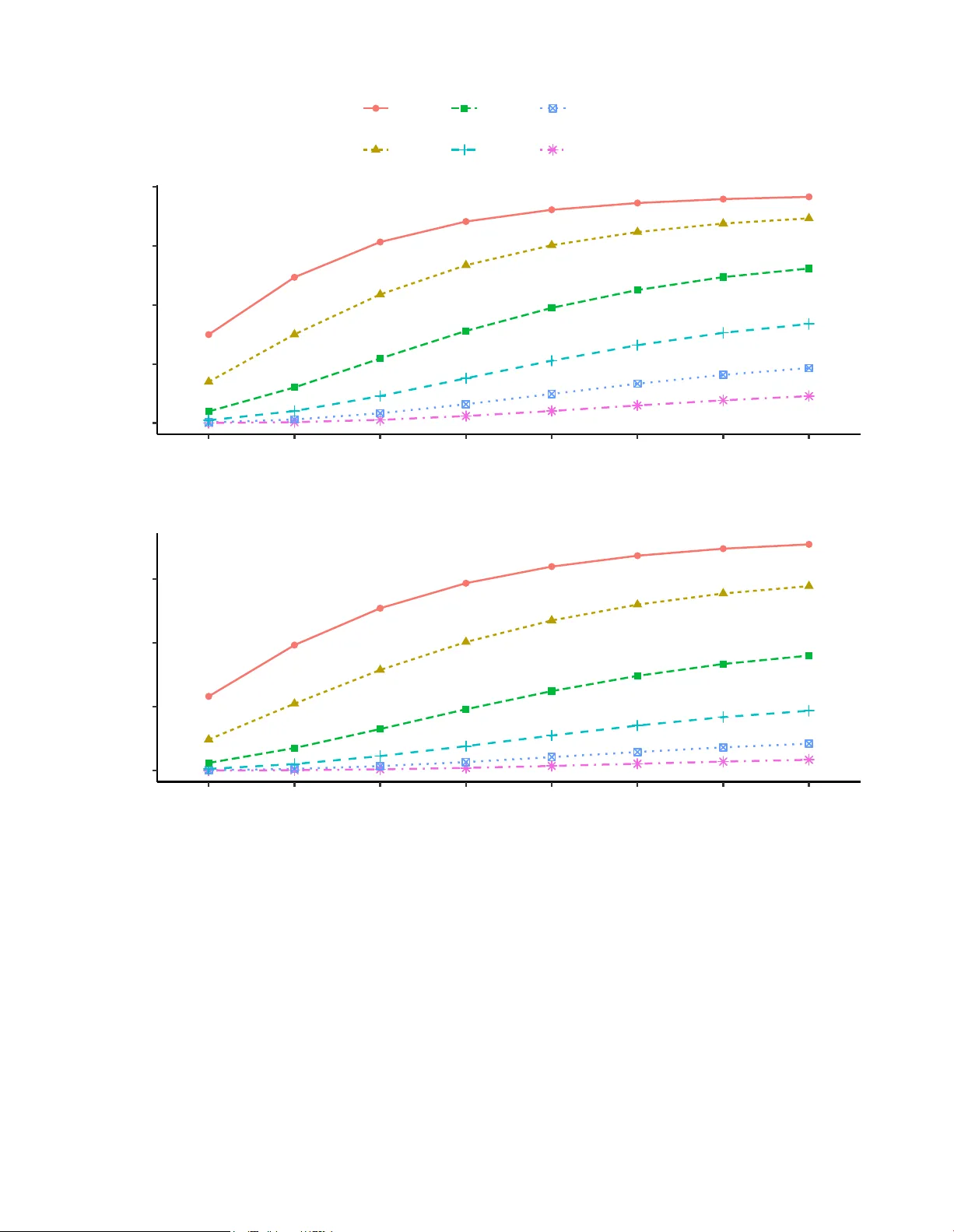
Sample size and p o w er determination for assessing o v erall SNP effects in join t mo deling of longitudinal and time-to-ev en t data Y uan Bian 1,2,3 and Shelley B. Bull 2,3 1 Dep artment of Biostatistics, Columbia University, Unite d States 2 Division of Biostatistics, Dal la L ana Scho ol of Public He alth, University of T or onto, Canada 3 Lunenfeld-T anenb aum R ese ar ch Institute, Sinai He alth, Canada Abstract Longitudinal biomarkers are frequen tly collected in clinical studies due to their strong asso- ciation with time-to-even t outcomes. While considerable progress has b een made in metho ds for jointly mo deling longitudinal and surviv al data, comparativ ely little attention has b een paid to statistical design considerations, particularly sample size and p o wer calculations, in ge- netic studies. Y et, appropriate sample size estimation is essen tial for ensuring adequate p o w er and v alid inference. Genetic v ariants ma y influence ev en t risk through b oth direct effects and indirect effects mediated b y longitudinal biomarkers. In this pap er, w e derive a closed-form sample size form ula for testing the ov erall effect of a single nucleotide p olymorphism within a join t modeling framew ork. Sim ulation studies demonstrate that the proposed form ula yields accurate and robust performance in finite samples. W e illustrate the practical utility of our metho d using data from the Diab etes Control and Complications T rial. Keywor ds: Genetic association; Joint mo deling; Longitudinal data; P ow er determination; Sample size; Surviv al analysis 1 1 In tro duction Diab etes, characterized b y chronically elev ated bloo d glucose lev els, is among the most prev alen t and rapidly increasing c hronic diseases w orldwide. In 2021, an estimated 38 . 4 million Americans, appro ximately 11 . 6% of the U.S. population, w ere living with diab etes (Cen ters for Disease Con trol and Preven tion, 2021). Globally , the num b er of adults with diab etes is pro jected to reach 693 million b y 2045, a more than 50% increase from 2017 levels (Cho et al., 2018). As a leading cause of death, diab etes is asso ciated with a wide range of long-term complications, including microv ascular conditions (e.g., nephropathy , retinopa- th y , and neuropathy) and macrov ascular diseases (e.g., cardiov ascular disease and stroke) (Papatheodorou et al., 2018). These complications con tribute substantially to increased mortalit y , blindness, kidney fail- ure, and reduced quality of life (Morrish et al., 2001). T yp e 1 diab etes, also known as insulin-dep endent diab etes mellitus, results from the pancreas’s inabilit y to pro duce sufficien t insulin. Individuals with t yp e 1 diabetes require lifelong insulin therapy to main tain normoglycemia (Chiang et al., 2014). Although its precise etiology remains unclear, it is widely b eliev ed to in volv e complex in teractions b etw een genetic and en vironmen tal factors (Cole and Florez, 2020). Because p o or glycemic con trol is a ma jor risk factor for diab etes-related complications (Kn uiman et al., 1986), a key scien tific question is whether genetic v ariants influence the timing of these complications through glycemic path w a ys, typically measured via hemoglobin A1c (HbA1c), or through alternativ e mech- anisms. Addressing this question requires a study design with adequate statistical p ow er, as sample size directly impacts the precision of parameter estimates and the ability to detect meaningful genetic effects. Ho w ev er, practical constraints often limit data collection, making rigorous sample size estimation a critical comp onen t of study design. Sev eral statistical approaches ha v e b een developed for sample size estimation in surviv al analysis. Sc ho enfeld (1983) introduced a widely used form ula based on the Cox prop ortional hazards mo del for comparing tw o randomized groups. Other contributions include log-rank test–based approac hes (F reed- man, 1982; Lak atos, 1988), and metho ds for non-binary co v ariates under exp onential surviv al assumptions (Zhen and Murphy, 1994). Hsieh and Lav ori (2000) extended Schoenfeld’s form ula to accommo date con- tin uous and categorical cov ariates without assuming an exp onential surviv al distribution. More recently , Chen et al. (2011) prop osed sample size formulas for the asso ciations b et ween longitudinal biomarkers and surviv al outcomes, as well as ov erall treatment effect. W ang et al. (2014) developed sample size form ula to incorp orate time-dep endent cov ariates in proportional hazards mo dels. 2 In genetic studies, the exp osure v ariable is often a single nucleotide p olymorphism (SNP), typically co ded as a dosage v ariable with three levels (e.g., 0, 1, or 2 copies of a risk allele). Dep ending on the minor allele frequency , genotype distribution may b e highly un balanced, p otentially reducing statistical efficiency and affecting the v alidity of asymptotic approximations. Moreo v er, unlike treatment effects, which are generally assumed to b e directional (b eneficial or harmful), genetic effects can increase or decrease the risk or timing of an ev ent, necessitating tw o-sided hypothesis testing. In this pap er, we derive a closed-form sample size form ula for testing the o v erall SNP effect within a join t modeling framew ork for longitudinal and surviv al data. W e further dev elop ed an in teractiv e Shin y app to determine sample size and p o w er, av ailable at https://krisyuanbian.shinyapps.io/PowerSNP/ . Our metho d extends the approach developed by Chen et al. (2011) to accommo date non-binary cov ariates such as SNPs. W e illustrate the utility of our approach using data from the Diab etes Con trol and Complications T rial (DCCT; The DCCT Researc h Group, 1986, 1990), a m ulticenter randomized con trolled clinical trial initiated in 1983 that enrolled 1,441 individuals with t yp e 1 diab etes. P articipan ts were randomized to receiv e either in tensiv e insulin therapy or conv entional treatmen t and were follo w ed for an av erage of 6.5 y ears. The study collected ric h longitudinal data on glycemic con trol (e.g., quarterly HbA1c measuremen ts) and detailed time-to-even t data on diab etic complications such as retinopathy . A genome-wide asso ciation study (GW AS) b y P aterson et al. (2010) iden tified sev eral SNPs asso ciated with these complications in both treatmen t arms. Our analysis suggests that for either treatment arm, the DCCT sample size is insufficient to achiev e adequate p ow er at conv entional GW AS significance levels. The remainder of this pap er is organized as follows. Section 2 introduces the join t mo deling framework and presen ts our new sample size form ula for assessing o v erall SNP effects. Section 3 ev aluates the accuracy and robustness of the prop osed form ula under v arying parameter settings and visit sc hedules. In Section 4, w e apply the metho dology to the DCCT data and demonstrate its practical utility . W e conclude with a discussion in Section 5. 2 Metho ds 2.1 Preliminaries and Notation F or sub ject i = 1 , . . . , n , let ˜ T i and C i denote the even t and censoring times, resp ectiv ely . Define the observ ed time as T i = min( ˜ T i , C i ) and the even t indicator as ∆ i = 1 ( ˜ T i ≤ C i ). Let SNP i represen t the 3 genot yp e for a selected single n ucleotide polymorphism (SNP), co ded as { 0 , 1 , 2 } , corresp onding to homozy- gous reference, heterozygous, and homozygous minor genot yp es. Under the assumption of Hardy–W ein b erg equilibrium, the genot yp e frequencies follo w ( q 2 , 2 pq , p 2 ), where p and q = (1 − p ) denote the minor and ma- jor allele frequencies, resp ectively . Let Y i ( t ) denote the observed longitudinal measuremen t at time t ≥ 0, recorded intermitten tly up to T i . This pro cess is sub ject to measurement error, with η i ( t ) representing the unobserv ed true underlying tra jectory . The joint mo deling framework links tw o sub-models, one for the longitudinal pro cess Y i ( t ) and one for the time-to-even t outcome T i , by incorp orating the true longitudinal tra jectory into the hazard function. F or the surviv al pro cess, w e assume a prop ortional hazards mo del of the form: λ i ( t ) = λ 0 ( t ) exp { γ g SNP i + αη i ( t ) } , (1) where λ 0 ( t ) is the baseline hazard, γ g represen ts the direct effect of the SNP on the hazard, and α quan tifies the asso ciation b etw een the true longitudinal tra jectory and the even t risk. The observed longitudinal outcome is mo deled as: Y i ( t ) = η i ( t ) + ϵ i ( t ) where ϵ i ( t ) ∼ N (0 , σ 2 e ) represents indep endent measurement errors across time and sub jects. The true tra jectory η i ( t ) is mo deled as a sub ject-sp ecific polynomial function of time: η i ( t ) = ( β 0 + b i 0 ) + ( β 1 + b i 1 ) t + ( β 2 + b i 2 ) t 2 + · · · + ( β q + b iq ) t q + β g SNP i , (2) where β i = ( β 0 , β 1 , · · · , β q , β g ) ⊤ are fixed effects and b i = ( b i 0 , b i 1 , · · · , b ⊤ iq ) ∼ N (0 , Σ) are sub ject-sp ecific random effects capturing individual deviations from the p opulation-level tra jectory . The random effects are assumed to b e indep endent of the measuremen t error. Substituting (2) in to the hazard mo del yields: λ i ( t ) = λ 0 ( t ) exp [( γ g + αβ g )SNP i + α { ( β 0 + b i 0 ) + ( β 1 + b i 1 ) t + · · · + ( β q + b iq ) t q } ] . In this framework, β g reflects the SNP’s effect on the longitudinal tra jectory , while γ g captures its direct effect on the hazard. The term αβ g represen ts the SNP’s indirect effect on the hazard mediated through 4 the longitudinal pro cess. Thus, γ g + αβ g quan tifies the SNP’s ov erall effect on ev ent risk, com bining b oth direct and indirect (longitudinally mediated) contributions. Our primary interest lies in testing this o v erall effect, i.e., whether γ g + αβ g = 0. 2.2 Sample Size and P o w er Determination for the Ov erall SNP Effect T o assess the o verall SNP effect, w e test the n ull h yp othesis H 0 : γ g + αβ g = 0 against the alternativ e H a : γ g + αβ g  = 0. While Chen et al. (2011) prop osed a sample size formula for detecting ov erall treatmen t effects in joint mo dels, SNPs present unique challenges: they are categorical with three levels (e.g., 0, 1, or 2 copies of the minor allele) and bidirectional in nature. Consequently , a tw o-sided test is more appropriate when ev aluating genetic effects. F ollo wing Schoenfeld (1983) and Chen et al. (2011), the num b er of even ts D required to ac hiev e p ow er 1 − ˜ β at a tw o-sided significance lev el ˜ α is given by: D = ( Z 1 − ˜ β + Z 1 − ˜ α/ 2 ) 2 2 pq ( γ g + αβ g ) 2 , (3) where Z 1 − ˜ α/ 2 and Z 1 − ˜ β are quantiles of the standard normal distribution corresp onding to the desired significance level and p ow er, respectively . This formula parallels the classical treatment-effect sample size expression, substituting the binary treatmen t v ariance with the SNP genotype v ariance 2 pq , and adjusting for tw o-sided testing by using ˜ α/ 2. It pro vides a practical to ol for determining the num b er of even ts required to detect SNP effects of v arying magnitude and allele frequencies. As sho wn in (3), the required num b er of even ts D is in v ersely prop ortional to b oth the genot yp e v ariance 2 pq and the squared ov erall SNP effect size ( γ g + α β g ) 2 . Consequen tly , SNPs with lo wer minor allele frequencies (i.e., smaller p ) or smaller o verall effect sizes necessitate larger sample sizes to achiev e adequate p o wer. These relationships highlight the imp ortance of accounting for b oth allele frequency and effect magnitude when assessing study feasibility , esp ecially when targeting rare v ariants or mo dest genetic effects. T o compute the p ow er for given n um b ers of even ts and effect size, we inv ert the sample size formula: 1 − ˜ β = Φ  p 2 pq D ( γ g + αβ g ) − Z 1 − ˜ α/ 2  (4) where Φ( · ) denotes the cum ulativ e distribution function of the standard normal distribution. (4) shows 5 that p ow er increases with larger v alues of D , γ g + αβ g , or genotype v ariance 2 pq , and decreases as the effect size or allele frequency diminishes. In addition, a more stringent significance threshold, such as when correcting for m ultiple comparisons in genome-wide studies, increases Z 1 − ˜ α/ 2 , thereb y reducing p ow er for a fixed sample size. These trade-offs underscore the need to balance p ow er and false p ositive control, particularly in studies designed to detect mo dest genetic effects or rare v ariants. When D is unobserv ed in sim ulations, w e approximate p o w er by replacing D with its empirical estimate ¯ D , the av erage n um b er of ev en ts observed. 2.3 Calculating Empirical p o w er for the Ov erall SNP Effect T o v alidate the calculated p o w er, we estimate the empirical p o wer as the proportion of simulation replicates in whic h the null h yp othesis is rejected at the significance lev el ˜ α (that is, when the p-v alue is less than or equal to ˜ α ). Direct join t modeling (JM) approaches for estimating and testing the o verall SNP effect can b e computationally intensiv e and challenging, as they typically rely on the Exp ectation-Maximization (EM) algorithm (Rizop oulos, 2012). These challenges are comp ounded as the num b er of time p oints or sample size increases, leading to substan tially longer computation times. In light of these limitations, t w o-stage metho ds provide a practical alternativ e to JM by significantly reducing computational burden, particularly in genome-wide settings (Canouil et al., 2018). Based on these considerations, we prop ose the follo wing tw o-stage approach to estimate the o v erall SNP effect. T o ev aluate the ov erall SNP effect in practice, we first fit the full longitudinal model to estimate β g . Us- ing this estimate, w e compute adjusted longitudinal resp onses as y ′ i ( t ) = y i ( t ) − ˆ β g SNP i , effectiv ely remo ving the SNP-related v ariation from the observed measurements. W e then fit a reduced longitudinal mo del of the form: y ′ i ( t ) = η ′ i ( t ) + ϵ ′ i ( t ) to estimate the adjusted tra jectory η ′ i ( t ), which is indep enden t of SNP effects. Next, we fit a surviv al mo del incorp orating the adjusted tra jectory: λ i ( t ) = λ 0 ( t ) exp { θ g SNP i + α ′ ˆ η ′ i ( t ) } , where θ g estimates the ov erall SNP effect on the hazard, and α ′ quan tifies the asso ciation b et w een the ad- justed longitudinal tra jectory and surviv al risk. The significance of the ov erall SNP effect is assessed under the null hypothesis H 0 : θ g = 0, and empirical p ow er is calculated based on the prop ortion of rejections across simulated datasets. 6 3 Sim ulation Studies W e ev aluate the finite-sample p erformance of the prop osed sample size formula through simulation studies. A range of simulated data is used to assess its accuracy in estimating required sample sizes under v arying conditions, including different p o w er lev els, significance thresholds, visit sc hedule, random effect, and SNP effect sizes. F or each parameter configuration describ ed b elow, 1000 simulations are conducted with a fixed sample size of 1000. 3.1 Sim ulation Design and Data Generation W e b egin by discretizing time ov er a presp ecified grid t grid . F or sub ject i , we simulate the genot yp e v ariable SNP i from the set { 0 , 1 , 2 } with probabilities (0 . 49 , 0 . 42 , 0 . 09), resp ectively . F or the longitudinal pro cess, sub ject-sp ecific random effects b i = ( b i 0 , b i 1 ) are drawn from a biv ariate normal distribution with mean zero and cov ariance matrix Σ. The cov ariance matrix Σ is parameterized b y δ 2 0 , δ 2 1 , and δ 0 , 1 , rep- resen ting the v ariance of the random intercept, the v ariance of the random slop e, and their cov ariance, resp ectiv ely . The true underlying longitudinal tra jectory for sub ject i at time t is given by η i ( t ) = ( β 0 + b i 0 ) + ( β 1 + b i 1 ) t + β 2 t 2 + β g · SNP i . This function is ev aluated at all scheduled time p oints t grid . Observed longitudinal measurements are then sim ulated as y i ( t ) ∼ N ( η i ( t ) , 0 . 7). The surviv al pro cess is defined via the sub ject-sp ecific hazard function λ i ( t ) defined in (1), with the corresp onding surviv al function S i ( T ) = exp  − R T 0 λ i ( u ) du  . T o simulate even t times, we follow the approac h of Austin (2012), dra wing p i ∼ Uniform(0 , 1) and solving for the laten t even t time ˜ T i suc h that p i = exp − Z ˜ T i 0 λ i ( u ) du ! . If the cumulativ e hazard function is linear in time, a closed-form solution for ˜ T i is a v ailable; otherwise, we apply the bisection metho d to n umerically solve for ˜ T i within the in terv al [0 , 100]. Censoring times C i are dra wn from a uniform distribution ov er the latter half of the study p erio d to reflect staggered entry and administrativ e censoring. The observed surviv al time is defined as T i = min( ˜ T i , C i ). F or each sub ject, w e iden tify t L as the largest time p oint in t grid less than T i , and t U as the smallest time p oint greater than T i . 7 Ev en ts or censoring are assumed to o ccur within the in terv al ( t L , t U ], and surviv al information is retained only up to t U . This en tire simulation procedure is rep eated indep endently for eac h sub ject. All unsp ecified parameters will b e defined in the next section, corresp onding to differen t settings and scenarios. Unless otherwise stated, a significance level of 0 . 05 is used. 3.2 Sim ulation Results T able 1 demonstrate that the sample size formula provides reliable estimates when the primary goal is to assess the ov erall SNP effect. Imp ortantly , the p o wer is largely unaffected by differen t random effect parameters δ 2 0 , δ 2 1 , and δ 0 , 1 in the longitudinal pro cess. The formula consistently appro ximates the required sample size across different v alues of α , β g , and γ g , indicating its robustness in handling a v ariety of parameter settings. T able 1: V alidation of sample size formula for testing the ov erall SNP effect for v arying cov ariance structure, genetic effects, and asso ciation parameter P ow er α β g γ g γ g + αβ g δ 2 0 δ 2 1 δ 0 , 1 ¯ D Empirical Calculated 0.25 0.3 0.1 0.175 2 1 -0.1 610.21 0.787 0.800 0.25 0.3 0.1 0.175 2 0.5 -0.6 616.49 0.798 0.804 0.25 0.3 0.1 0.175 2 0.5 -0.1 610.21 0.801 0.800 0.25 0.3 0.1 0.175 2 0.1 -0.3 608.66 0.802 0.799 0.25 0.3 0.1 0.175 2 0.1 -0.1 607.12 0.809 0.798 0.25 0.1 0.05 0.075 2 0.1 -0.1 586.98 0.226 0.217 0.25 0.1 0.1 0.125 2 0.1 -0.1 597.41 0.509 0.508 0.25 0.5 0.1 0.225 2 0.1 -0.1 617.86 0.956 0.952 0.15 0.3 0.1 0.145 2 0.1 -0.1 321.85 0.415 0.392 0.15 0.3 0.2 0.245 2 0.1 -0.1 338.69 0.845 0.832 The longitudinal part is measured quarterly , and surviv al part is measured half y early . The even t time is simulated from W eibull distribution with λ = 0 . 01, v = 1 . 1; And β 0 = 8 . 5, β 1 = 0 . 1, β 2 = 0. Additionally , T able 2 shows that the sample size form ula performs well across a wide range of significance lev els. The form ula remains relatively insensitiv e to the frequency of measurements (S1 – S4) as long as there are a sufficien t num b er of measurements p er sub ject. Ho wev er, the p erformance of the form ula declines when the n um b er of measurements is very small. Specifically , comparing S4 and S5 highligh ts that p o w er underestimation arises in cases of interv al censoring, which affects the accuracy of the sample 8 size estimates when few er measurements are a v ailable. Ov erall, these simulation studies confirm that the sample size form ula is effective in most scenarios but ma y require adjustments when dealing with limited data. T able 2: V alidation of sample size formula for testing the ov erall SNP effect for v arying n umbers of visits and significance lev els P ow er Calculated Empirical Significance Lev el S1 S2 S3 S4 S5 5 × 10 − 2 0.978 0.961 0.968 0.958 0.946 0.908 10 − 2 0.919 0.891 0.903 0.880 0.863 0.798 10 − 3 0.753 0.723 0.709 0.674 0.670 0.546 10 − 4 0.533 0.551 0.508 0.495 0.442 0.312 10 − 5 0.329 0.359 0.349 0.300 0.270 0.161 10 − 6 0.179 0.211 0.202 0.167 0.141 0.072 10 − 7 0.088 0.118 0.114 0.107 0.070 0.031 10 − 8 0.039 0.067 0.061 0.054 0.026 0.008 S1: Quarterly longitudinal visit & half year time to even t visit, S2: Half year longitudinal visit & yearly time to even t visit; S3: Y early longitudinal visit & six time to even t visit, S4: Five longitudinal visit & fiv e time to even t visit, S5: Five longitudinal visit & three time to even t visit. The even t time is simulated from W eibull distribution with λ = 0 . 001, v = 1 . 1; And β 0 = 8 . 5, β 1 = 0 . 1, β 2 = 0, α = 0 . 5, β g = 0 . 3, γ g = 0 . 1, δ 2 0 = 2, δ 2 1 = 0 . 1, δ 0 , 1 = − 0 . 1. The mean num b er of even ts observ ed in 1000 simulation replicates, ¯ D , is 601 . 64 based on simulation. The simulation studies presented in T able 3 compare the p ow er when the longitudinal mo del is mis- sp ecified. When the true quadratic mo del is correctly sp ecified, the empirical p o w er closely aligns with the calculated p o w er, demonstrating that the mo del captures the underlying data structure accurately . Ho w- ev er, when the longitudinal model is misspecified as linear, the empirical p o w er deviates from the calculated p o w er. This discrepancy arises b ecause the true longitudinal tra jectory exhibits additional curv ature (i.e., an increase in β 2 ), which the linear mo del fails to capture. As a result, the linear mo del underestimates the complexit y of the data, leading to a reduced empirical p ow er compared to the calculated p ow er. This high- ligh ts the imp ortance of correctly sp ecifying the longitudinal mo del to ensure accurate p ow er estimation and reliable conclusions in h yp othesis testing. 9 T able 3: Comparison of empirical p o w er to detect the ov erall SNP effect under missp ecified longitu- dinal mo dels, with β 2 represen ting the magnitude of nonlinear curv ature in the longitudinal pro cess P ow er α β g γ g γ g + α β g ¯ D β 2 Empirical Empirical* Calculated 0.35 0.2 0.05 0.12 426.91 0.1 0.355 0.351 0.362 0.35 0.2 0.05 0.12 562.47 0.15 0.427 0.411 0.454 0.35 0.2 0.05 0.12 689.97 0.2 0.515 0.461 0.533 The longitudinal part is measured quarterly , and surviv al part is measured half y early . The even t time is simulated from W eibull distribution with λ = 0 . 003, v = 1 . 15; β 0 = 7 . 5, β 1 = − 0 . 5, δ 2 0 = 1, δ 2 1 = 0 . 3, δ 2 2 = 0 . 01. Empirical is based on fitting quadratic (true) longitudinal mo del, Empirical* is based on fitting linear (missp ecified) longitudinal mo del. 3.3 Biased estimates of the SNP effect when ignoring the longitudinal tra jectory When a SNP influences the longitudinal pro cess (i.e., β g  = 0 in (2)), and the longitudinal pro cess in turn affects the time-to-even t outcome (i.e., α  = 0 in (1)), the total effect of the SNP on the surviv al outcome is given by γ g + αβ g . It is well known that omitting the longitudinal pro cess from the surviv al mo del in (1) can lead to biased estimation of γ g . Even when the SNP is not associated with the longitudinal pro cess (i.e., β g = 0), failure to account for the longitudinal tra jectory can still induce attenuation bias in estimating γ g due to unobserved heterogeneity (Horowitz, 1999; Abbring and V an Den Berg, 2007). T able 4 presents the bias in estimating γ g under the null scenario where β g = 0, comparing v arious mo deling strategies: the Co x mo del that excludes the longitudinal pro cess, tw o-stage metho ds (using either kno wn or estimated tra jectories), and the joint likelihoo d approach. The degree of bias is ev aluated as a function of the asso ciation strength α b etw een the longitudinal and surviv al pro cesses. T o ensure comparable even t rates across scenarios, we set λ = 0 . 01 for α = 0 . 25, and λ = 0 . 001 for α = 0 . 4 and 0 . 5. As α increases, the Cox mo del that omits the longitudinal process exhibits increasingly severe bias due to the unaccounted asso ciation. In contrast, b oth t wo-stage metho ds and the joint lik eliho o d approac h yield acceptable results. Interestingly , the tw o-stage metho ds sligh tly outp erform the joint approach, aligning with prior findings that t w o-stage estimators can offer greater robustness under certain conditions (Chen et al., 2011). 10 T able 4: Effect of the v alue of α on the estimation of direct SNP effect γ g on surviv al based on differen t analysis metho ds: Separate, tw o stage and joint likelihoo d Analysis mo del λ i ( t ) = λ 0 ( t ) exp( γ g SNP i ) λ i ( t ) = λ 0 ( t ) exp { γ g SNP i + α (( β 0 + b i 0 ) + ( β 1 + b i 1 ) t ) } α ˆ γ g based on co x partial lik eliho o d ˆ γ g based on kno wn tra jectory ˆ γ g based on Tw o Stage ˆ γ g based on join t lik eliho o d 0.25 0.093(0.002) 0.101(0.002) 0.101(0.002) 0.096(0.002) 0.4 0.090(0.003) 0.102(0.003) 0.101(0.003) 0.096(0.003) 0.5 0.077(0.002) 0.100(0.002) 0.100(0.002) 0.095(0.002) The longitudinal part is measured quarterly , and surviv al part is measured half y early . The even t time is simulated from W eibull distribution with λ , v = 1 . 1; And β 0 = 8 . 5, β 1 = 0 . 1, δ 2 0 = 2, δ 2 1 =0.1, δ 0 , 1 = − 0 . 1. T rue γ g = 0 . 1. And ˆ γ g is summarized as mean (SD) based on 1000 simulations of 1000 sub jects. ˆ γ g . 3.4 Relationship b et ween the calculated p o w er and the sample size, maxim um follow-up time, and other k ey parameters W e further inv estigate how the calculated p ow er v aries with sample size, ev en t size, maxim um follo w- up time, and other key parameters using the prop osed sample size formula for the ov erall SNP effect. Unless otherwise sp ecified, the maxim um follow-up time is set to 10 y ears, with longitudinal measurements collected quarterly and surviv al outcomes assessed semi-annually; ev en t times are simulated from a W eibull distribution with shap e parameter v = 1 . 1 and scale parameter λ = 0 . 01. The following mo del parameters are used: β 0 = 8 . 5, β 1 = 0 . 1, p = 0 . 3, δ 2 0 = 2, δ 2 1 = 0 . 1, δ 0 , 1 = − 0 . 1, γ g = 0 . 1, α = 0 . 25, and β g = 0 . 3. The sample sizes and corresp onding estimated num b ers of even ts, denoted by ¯ D , are summarized in T ables 5, 6, and 7, resp ectively . Figures 1, 2, and 3 display the calculated p ow er as a function of ¯ D and sample size, across different follow-up times and v arying v alues of α and γ g . Figure 1 presents the p ow er curv es for the ov erall SNP effect at three follow-up times: 5, 7.5, and 10 y ears. The results rev eal a clear pattern: for a fixed sample size, longer follow-up times yield higher p o w er. This is b ecause extended follow-up allows for the accum ulation of more surviv al data through additional observ ed ev en ts. As more information b ecomes a v ailable o ver time, the statistical p ow er to detect the effect increases. When plotting p o w er against ¯ D , the curves collapse into a single tra jectory , consisten t with the relationship describ ed in (4). Figures 2 and 3 further illustrate how b oth α and γ g affect ¯ D and, consequently , p ow er. Figure 2 shows p o w er curves for three v alues of α : 0.15, 0.25, and 0.5. As exp ected, p ow er decreases with smaller α at the 11 Time 10 5 7.5 0.2 0.4 0.6 0.8 200 400 600 D P ower 0.2 0.4 0.6 0.8 250 500 750 1000 Sample Size P ower Figure 1: Po wer curve at different follow-up times T able 5: Corresp onding ¯ D v alues for Figure 1 F ollowup Sample Size 100 200 300 400 500 600 700 800 900 1000 5 35.26 70.34 105.46 140.33 175.24 210.38 245.54 280.86 315.88 351.15 7.5 49.36 98.67 148.12 197.35 246.71 296.15 345.663 395.25 444.49 493.90 10 60.86 121.66 182.52 243.30 303.91 364.69 425.38 486.28 546.85 607.51 D is the mean num b er of even ts observed in simulation replicates. same sample size, reflecting the fact that weak er effects require larger samples to ac hiev e the same p ow er. When p ow er is plotted against ¯ D , the curves no longer align due to v ariation in b oth ¯ D and α in (4). The p o w er still declines with decreasing α for a given ¯ D . Similarly , Figure 3 displays p ow er curves for three v alues of γ g : 0.05, 0.1, and 0.2. As with α , smaller v alues of γ g result in lo wer p o w er at the same sample size or ¯ D , again underscoring that smaller effect sizes necessitate larger samples. The patterns observed in Figures 2 and 3 are analogous, as b oth α and γ g con tribute to the ov erall effect size, which in turn influences the sample size form ula. 12 α 0.15 0.25 0.5 0.25 0.50 0.75 1.00 0 250 500 750 1000 D P ower 0.25 0.50 0.75 1.00 250 500 750 1000 Sample Size P ower Figure 2: Po wer curve when only α v aries T able 6: Corresp onding ¯ D v alues for Figure 2 α Sample Size 100 200 300 400 500 600 700 800 900 1000 0.15 32.30 64.46 96.62 128.54 160.68 192.87 225.24 257.56 289.70 321.87 0.25 60.86 121.66 182.52 243.30 303.91 364.69 425.38 486.28 546.85 607.51 0.5 98.25 196.49 294.71 392.95 491.22 589.51 687.72 785.94 884.15 982.35 D is the mean num b er of even ts observed in simulation replicates. T able 7: Corresp onding ¯ D v alues for Figure 3 γ g Sample Size 100 200 300 400 500 600 700 800 900 1000 0.05 59.89 119.76 179.57 239.35 299.01 358.77 418.46 478.38 537.97 597.63 0.1 60.86 121.66 182.52 243.30 303.91 364.69 425.38 486.28 546.85 607.51 0.2 62.79 125.47 188.23 250.89 313.47 376.18 438.83 501.68 564.20 626.85 D is the mean num b er of even ts observed in simulation replicates. 13 γ g 0.05 0.1 0.2 0.25 0.50 0.75 1.00 200 400 600 D P ower 0.25 0.50 0.75 1.00 250 500 750 1000 Sample Size P ower Figure 3: Po wer curve when only γ g v aries 4 Retrosp ectiv e P o w er Analyses for the Diab etes Con trol and Complications T rial T o demonstrate the application of the prop osed sample size formula, w e conducted a retrosp ective p o w er analysis using data from the Diab etes Control and Complications T rial (DCCT; The DCCT Re- searc h Group, 1986, 1990). The DCCT was a prosp ective, randomized controlled clinical trial designed to compare the effects of intensiv e versus conv entional treatment on the onset and progression of long- term microv ascular and neurological complications in individuals with type 1 diab etes. Under conv entional treatmen t, patients received one or tw o daily injections of a com bination of intermediate- and short-acting insulin. They p erformed daily self-monitoring of urine or blo o d glucose levels, receiv ed education on diet and exercise, but typically did not adjust insulin dosages on a daily basis. In contrast, patients in the in tensiv e treatment arm receiv ed insulin three or more times daily via injection or external pump. Insulin doses were adjusted based on self-monitoring of blo o d glucose lev els p erformed at least four times p er day , dietary in take, and anticipated physical activity . The treatmen t ob jectiv e in the intensiv e arm was to main tain HbA1c levels within the normal range, defined as less than 6.05 p ercent (The DCCT Research Group, 1993). Ov er a follow-up p erio d ranging from three to nine years, with a mean duration of 6.5 y ears, the 14 con v en tional arm maintained an av erage hemoglobin A1C (HbA1c) level of approximately 9.0 p ercen t, consisten t with their baseline v alues. The in tensiv e arm achiev ed and sustained a mean HbA1c level of appro ximately 7.0 p ercent. HbA1c, a measure of long-term glycemic exp osure, w as collected quarterly in the conv entional arm and monthly in the in tensiv e arm. Sub jects in the conv entional arm had an av erage of 17.26 quarterly measurements, with a minimum of 3, a median of 17.5, and a maximum of 37. Sub jects in the intensiv e arm had an av erage of 18.35 quarterly measuremen ts, with a minimum of 3, a median of 19, and a maximum of 38. Clinical complications w ere assessed through p erio dic ev aluations, with retinopathy status determined b y grading retinal photographs tak en at semiann ual visits ov er a maxim um duration of ten years. Retinopa- th y was selected as the primary outcome due to its well-c haracterized natural history and reliable assessmen t (The DCCT Research Group, 1990). The primary endpoint for this analysis is the time from study entry to the onset of mild retinopathy . Sub jects with retinopathy diagnosed at baseline were excluded for our analysis. Censoring was administrativ e and determined by a predefined calendar date. With the developmen t of genome-wide asso ciation study (GW AS) metho dologies, DCCT participants underw en t genotyping using the Illumina 1M b eadchip assa y . After quality control procedures, a total of 841,342 SNPs with minor allele frequency greater than one p ercent w ere retained for analysis. Paterson et al. (2010) iden tified a ma jor lo cus near SOR CS1 on c hromosome 10q25.1 that w as significan tly asso ciated with HbA1c lev els in the con v ention al arm, with replication in the in tensiv e arm. Other lo ci nearing genome-wide significance included regions at 14q32.13 ( GSC ) and 9p22 ( BNC2 ) in the combined treatmen t arms, and 15q21.3 ( WDR72 ) in the in tensiv e arm. Some of these lo ci w ere also asso ciated with diabetic complications, notably BNC2 , which was linked to both renal and retinal outcomes. The direction of asso ciation at this lo cus w as consisten t with its effect on HbA1c: genotypes asso ciated with higher HbA1c levels were also asso ciated with increased complication risk. Due to substantiv e differences in treatment proto cols and outcomes, and in accordance with most prior analyses of the DCCT, we conducted separate p ow er analyses for each treatmen t arm. The conv en tional treatmen t group included 526 sub jects, among whom 315 exp erienced the even t of interest. The intensiv e treatmen t group included 527 sub jects, with 232 observ ed ev ents. Figure 4 presen ts p o w er curves for b oth the conv en tional and in tensiv e treatmen t arms, assuming an o v erall SNP effect size of θ g = 0 . 30. The plots demonstrate how statistical p ow er dep ends jointly on the minor allele frequency p and the significance lev el ˜ α . In the conv entional arm, 80% p ow er is achiev ed when p > 0 . 20 under the standard significance level of ˜ α = 0 . 05. In contrast, for the intensiv e arm, where the 15 n um b er of even ts is lo wer, the same p ow er threshold is only reac hed when p ≈ 0 . 40 at ˜ α = 0 . 05. These results indicate that the DCCT sample size is insufficient to attain adequate p ow er under conv entional GW AS significance thresholds in either treatment arm. Notably , the intensiv e arm exhibits greater sensitivit y to b oth allele frequency and the choice of ˜ α , reflecting the comp ounding effects of reduced sample size and ev en t rate on statistical p ow er. This underscores the imp ortance of considering study design factors, particularly sample size and even t accrual, when assessing the feasibility of detecting mo dest genetic effects in stratified analyses. 5 Discussion In this pap er, we prop ose a sample size formula sp ecifically designed for estimating the ov erall SNP effect within a joint mo deling framew ork. Our empirical results show that the formula pro vides accurate appro ximations across a wide range of scenarios, including v arying magnitudes of the SNP effect, differ- en t visit sc hedules, random effect structures, and significance levels. How ever, when the nu mber of visit sc hedules is to o small, the accuracy of the sample size estimates deteriorates. Additionally , we show that in v erting the sample size form ula to estimate the p ow er for detecting ov erall genetic effects p erforms well in simulation studies. T o demonstrate practical applicability , we conducted a retrospective p ow er analysis using data from the DCCT study . Notably , although we assume that the random effects and error terms in the longitudinal submo del follo w a normal distribution, the v alidit y of the sample size form ula itself do es not rely on this assumption. As demonstrated by Chen et al. (2011), the formula remains applicable in more general join t mo deling settings, thereby enhancing its practical utility in a wide range of genetic asso ciation studies in v olving longitudinal and time-to-ev ent data. Tw o key assumptions underlie the deriv ation and application of our sample size formula. First, it assumes that the longitudinal pro cess is sub ject to non-informativ e censoring. This is a critical condition, as the t w o-stage estimation procedure used in our deriv ation can produce biased results under informative censoring. Therefore, caution is warran ted when applying the form ula in settings where informative drop out may b e presen t. Second, when the longitudinal trait functions as a biomarker, w e assume that the indirect genetic effect on the surviv al outcome αβ g and the direct effect on the surviv al trait γ g act in the same direction. Violating this assumption ma y impact b oth the interpretation of genetic effects and the accuracy of p ow er estimation. In practice, the longitudinal submo del is often nonlinear and unknown, and the accuracy of the sample 16 α ~ 0.05 1e−2 1e−3 1e−4 1e−5 1e−6 0.00 0.25 0.50 0.75 1.00 0.05 0.10 0.15 0.20 0.25 0.30 0.35 0.40 p pow er Con v entional Ar m 0.00 0.25 0.50 0.75 0.05 0.10 0.15 0.20 0.25 0.30 0.35 0.40 p pow er Intensiv e Ar m Figure 4: Po wer curve when p and ˜ α v ary size form ula ma y b e influenced by how w ell the longitudinal pro cess is sp ecified. F or instance, as demon- strated b y Bian (2020), visualizations of the DCCT data reveal distinct tra jectories b et w een sub jects in the con trol and intensiv e treatment arms; and missp ecification of the longitudinal pro cess can lead to incorrect parameter estimation. Suc h differences emphasize the imp ortance of correctly mo deling the longitudinal trait, as missp ecification can lead to biased parameter estimates, affecting b oth the p ow er analysis and genetic effect estimation. This highligh ts a key challenge in applying the prop osed sample size form ula in 17 real-w orld studies: the mo del’s sensitivit y to inaccuracies in the sp ecification of longitudinal tra jectories. F urther exploration is needed to assess how mo del missp ecifications, such as incorrect assumptions ab out the tra jectories or error structures, may influence the v alidity of p ow er calculations and subsequent genetic asso ciation findings. Moreo v er, it w ould b e v aluable to in vestigate strategies for impro ving the robustness of the sample size formula when faced with mo del missp ecification, including alternative approac hes that can b etter accommo date v ariations in longitudinal tra jectories across different treatmen t groups or patient p opulations. Ac kno wledgemen ts This research is partially supp orted by a Canadian Institutes of Health Research (CIHR) pro ject grant. References Abbring, J. H. and V an Den Berg, G. J. (2007). The unobserved heterogeneity distribution in duration analysis. Biometrika , 94(1):87–99. Austin, P . C. (2012). Generating surviv al times to sim ulate cox prop ortional hazards mo dels with time- v arying co v ariates. Statistics in Me dicine , 31(29):3946–3958. Bian, Y. (2020). Hyp othesis T esting in Joint Mo dels for L ongitudinal and Time-to-Event Outc omes . Uni- v ersit y of T oronto. Canouil, M., Balk au, B., Roussel, R., F roguel, P ., and Ro cheleau, G. (2018). Join tly mo delling single n ucleotide p olymorphisms with longitudinal and time-to-even t trait: An application to type 2 diab etes and fasting plasma glucose. F r ontiers in Genetics , 9:210. Cen ters for Disease Con trol and Prev en tion (2021). National diab etes statistics rep ort. Accessed on May 13, 2025. Chen, L. M., Ibrahim, J. G., and Ch u, H. (2011). Sample size and p o wer determination in joint mo deling of longitudinal and surviv al data. Statistics in Me dicine , 30(18):2295–2309. Chiang, J. L., Kirkman, M. S., Laffel, L. M., and Peters, A. L. (2014). Type 1 diab etes through the life span: A p osition statement of the American Diab etes Asso ciation. Diab etes Car e , 37(7):2034. 18 Cho, N. H., Shaw, J. E., Karuranga, S., Huang, Y., da Ro cha F ernandes, J. D., Ohlrogge, A., and Malanda, B. (2018). Idf diab etes atlas: Global estimates of diab etes prev alence for 2017 and pro jections for 2045. Diab etes R ese ar ch and Clinic al Pr actic e , 138:271–281. Cole, J. B. and Florez, J. C. (2020). Genetics of diab etes mellitus and diab etes complications. Natur e R eviews Nephr olo gy , 16(7):377–390. F reedman, L. S. (1982). T ables of the n umber of patients required in clinical trials using the logrank test. Statistics in Me dicine , 1(2):121–129. Horo witz, J. L. (1999). Semiparametric estimation of a prop ortional hazard mo del with unobserved het- erogeneit y . Ec onometric a , 67(5):1001–1028. Hsieh, F. Y. and Lav ori, P . W. (2000). Sample-size calculations for the cox prop ortional hazards regression mo del with nonbinary cov ariates. Contr ol le d Clinic al T rials , 21(6):552–560. Kn uiman, M., W elb orn, T., McCann, V., Stanton, K., and Constable, I. (1986). Prev alence of diab etic complications in relation to risk factors. Diab etes , 35(12):1332–1339. Lak atos, E. (1988). Sample sizes based on the log-rank statistic in complex clinical trials. Biometrics , 44(1):229–241. Morrish, N., W ang, S.-L., Stevens, L., F uller, J., Keen, H., and Group, W. M. S. (2001). Mortalit y and causes of death in the who multinational study of v ascular disease in diab etes. Diab etolo gia , 44:14–21. P apatheo dorou, K., Banach, M., Bekiari, E., Rizzo, M., and Edmonds, M. (2018). Complications of diab etes 2017. Journal of Diab etes R ese ar ch , 2018:Article ID 3086167. P aterson, A. D., W aggott, D., Boright, A. P ., Hosseini, S. M., Shen, E., Sylvestre, M. P ., W ong, I., Bhara j, B., Cleary , P . A., Lachin, J. M., Belo w, J. E., Nicolae, D., Cox, N. J., Can t y , A. J., Sun, L., and Bull, S. B. (2010). A genome-wide asso ciation study identifies a no v el ma jor lo cus for glycemic control in type 1 diab etes, as measured b y b oth a1c and glucose. Diab etes , 59(2):539–549. Rizop oulos, D. (2012). Joint Mo dels for L ongitudinal and Time-to-Event Data: With Applic ations in R . CR C Press, Bo ca Raton. 19 Sc ho enfeld, D. (1983). Sample-size formula for the prop ortional-hazards regression mo del. Biometrics , 39(2):499–503. The DCCT Research Group (1986). The diab etes control and complications trial (DCCT): Design and metho dologic considerations for the feasibilit y phase. Diab etes , 35(5):530–545. The DCCT Research Group (1990). Diab etes control and complications trial (DCCT) up date. Diab etes Car e , 13(4):427–433. The DCCT Research Group (1993). The effect of in tensiv e treatment of diab etes on the dev elopment and progression of long-term complications in insulin-dep endent diab etes mellitus. New England Journal of Me dicine , 329(14):977–986. W ang, S., Zhang, J., and Lu, W. (2014). Sample size calculation for the prop ortional hazards mo del with a time-dep endent cov ariate. Computational Statistics and Data Analysis , 74:217–227. Zhen, B. and Murph y , J. R. (1994). Sample size determination for an exp onential surviv al model with an unrestricted cov ariate. Statistics in Me dicine , 13(4):391–397. 20