Joint analysis for multivariate longitudinal and event time data with a change point anchored at interval-censored event time

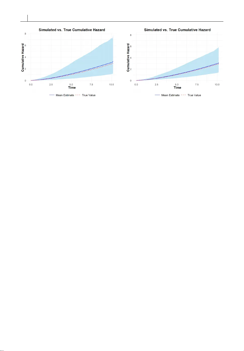
O R I G I N A L A R T I C L E J oint analysis f or multivariat e longitudinal and ev en t time data with a change point anchored at interv al-c ensored e v ent time Y ue Zhan 1 | Cheng Zheng 1 | Ying Zhang 1 1 Department of B iostatistics, College of Public Health, U niversity of N ebraska Medical Cent er, O maha, Nebraska, U nited States Correspondence Ying Zhang Email: ying.zhang@unmc.edu Funding information DHHS/NIH/NIGMS, Grant/ Aw ard Number: U54GM115458 Huntington ’s disease (HD ) is an autosomal dominant neu- rodeg enerative disorder characterized by motor dysfunc- tion, psychia tric disturban ces, and cognitive decline. The onset of HD is marked by sever e motor impairment, which may be pr edicted by prior cognitive decline and, in turn, ex - acerbate cognitiv e deficits. Clinical da ta, however , ar e o f- ten collected at discrete time points, so the timing o f dis- ease onset is subject to interval censoring. T o address the challenges posed by such data, we develop a joint model for multivariate longitudinal biomark ers with a change point anchored at an interv al-censor ed ev ent time. The model si- multaneously assesses the effects of longitudinal biomark- ers on the event time and the changes in biomark er trajec- tories following the event. W e conduct a c omprehensive simulation study to demonstrate the finite-sample perf or- mance of the proposed method for causal infer ence. Finally , we apply the method to PREDICT -HD, a multisite observa- tional cohort study of prodr omal HD individuals, to ascer- tain ho w c ognitive impairment and motor dysfunction in- teract during disease progression. K eywords — J oint model, Survival analysis, L ongitudi- nal biomarker , Change point, Interval-censor ed data Abbreviations: HD, Huntington’ s disease; MLE, Maximum Likelihood Estimation; DCL, Diagnose Confidence Level. 1 2 Y ue Zhan 1 | I N T R O D U C T I O N Huntington ’s disease (HD) is an inherited, autosomal dominant neurodegener ative disorder characterized by progr es- sive motor dysfunction, cognitive decline, and psy chiatric disturbances. The disease is caused by an abnormal ex- pansion of CAG trinucleotide repeats in the HTT gene on chromosome 4, which leads to the production of a mutant huntingtin protein that disrupts normal cellular function [1, 2]. Curr ently , there is no effectiv e treatment av ailable for HD patients. Huntington ’s disease encompasses motor , cognitive, and psychia tric manifestations, but the clinical diagnosis of onset is determined primarily by the emergence of motor symptoms [3]. Howe ver, cognitiv e impairment has been found to appear prior to HD motor diagnosis [4, 5, 6, 7, 8]. Zhang et al. [8] have thoroughly studied mild cognitive impairment (MCI) in various cognitive domains characterized by Harrington et al. [9], which is regarded as an early landmark for disease progr ession in prodromal HD individuals. Although a rapid cognitive decline at the early stage, attributed to the onset of HD, has been observed [10], an overar ching study of how cognitive impairment interacts with HD onset was lacking, but will be helpful to understand the HD progr ession in pr odromal HD individuals. In this work, we propose a holistic model to uncover the r elationship between cognitive decline in multiple domains and HD onset using joint modeling of multivaria te longitudinal and even t time data. Joint modeling of longitudinal and e vent time da ta has become increasingly important in biomedical studies, especially in chronic diseases, HIV / AIDS, cardio vascular research, etc, when understanding the interplay between longitudinal biomark ers and clinical events is crucial. The joint modeling framework was developed by simultane- ously modeling the longitudinal and event time data under a structure with shared subject-specific random eff ects [11, 12, 13, 14, 15, 16, 17]. R ecent developmen t of the joint modeling method allows resear chers to study the causal effect of the exposure on the survival outcome through the longitudinal marker [18, 19]. Pr evious work showed that by including both the random effect and the longitudinal marker in the survival model, the joint model frame- work allows the researcher to separat e the direct causal eff ect of the longitudinal mark er on the outcome and the time-independent unmeasured conf ounding between the marker and the outcome [20, 21]. The maximum likelihood method equipped with the EM algorithm has been a popular approach to estimate parameters in a joint model [22] for making statistical infer ences. It is worth noting that most of the joint models were developed for longitudinal biomarkers and right-censored event time, emphasizing either unbiased infer ence for event time outcome using time- dependent longitudinal biomarkers [13, 14, 23] or unbiased inferenc e of longitudinal trajectories of the biomarkers subject to informative drop-out [24, 25, 26]. These methods are not applicable to study the relationship between cognitive impairments and the HD onset in prodr omal HD individuals, which is subject to interval censoring brack eted by two adjacent motor diagnostic times, where the first time shows negative and the second time yields the motor diagnosis of HD. Although joint models of longitudinal biomarkers and interval-censor ed event times have been stud- ied more rec ently [27, 28, 29, 30], the methods did not concern the changes of longitudinal biomarkers triggered by the ev ent time. Some two-phase changing-point analyses of longitudinal data around an interval-censor ed event time have been explored [31, 32, 33], but they did not address how the longitudinal data impacted the interval-c ensored even t time. In addition, none of the afor ementioned approaches were concerned with causal inf erences. In this work, we propose a two-phase approach by extending the likelihood method for joint modeling of lon- gitudinal and interval-c ensored event time data to incorporate a potential change point in longitudinal biomarkers anchored at an unobserved event time, depicted in Figure (1), using the causal framework for the joint modeling [21]. The first phase of the model emphasizes how the longitudinal data impacts the event time, and the second phase investigat es whether /how the event time changes the trajectories of longitudinal biomarkers. We use an adaptive Newton-Raphson algorithm to compute the maximum lik elihood estimates (MLE) of all coefficients in this joint model, Y ue Zhan 3 and the nonparametric bootstr ap method to estimate the standard error of all estimated coefficients. F I G U R E 1 A hypothetical model for the HD disease progression: V and U are the two adjacent diagnosed times, with V being negative and U being positive for the HD diagnosis. The rest of this paper is organized as follows: in Section 2, we describe our notation, models, and the likelihood method for the causal two-phase joint modeling of changing-point longitudinal data and interval-censor ed even t time and illustrate how to calculate the MLE. In Section 3, we present simulation studies to evaluate the finite-sample performance of the proposed method. In Section 4, we apply our method to the data from the N eurobiological Predict ors of Huntington’s Disease Study (PREDICT -HD), a 12-year multisite prospective cohort study conducted between September 2002 and April 2014 [3] to examine the interplay between cognitiv e decline and the HD onset in prodromal HD individuals that cognitiv e declines pr edict the HD onset and the later accelerates cognitiv e declines. In Section 5, we summarize our findings and discuss potential extensions. 2 | M E T H O D S 2.1 | Nota tion First, we define notation for the observed data. W e consider K -dimensional longitudinal biomarker processes M ( t ) = ( M 1 ( t ) , M 2 ( t ) , · · · , M K ( t ) ) that are potentially pr edictive of the onset time of disease E , which is interval censored by ( V , U ] via periodic diagnoses, where V and U can be zer o and infinity, respectiv ely. Let X ( t ) be covariate pro- cesses that are potentially related to both longitudinal disease biomark ers and the onset time of disease. Assume the proc esses are assessed longitudinally at m random observa tion times T = ( t 1 , t 2 , · · · , t m ) , and the data fr om the processes collected at T are denoted as M = ( M ( t 1 ) , M ( t 2 ) , · · · , M ( t m ) ) and X = ( X ( t 1 ) , X ( t 2 ) , · · · , X ( t m ) ) . The observed data for an individual consist of D = ( m , T ; M , X ; V , U ) , and we have a total of n i.i.d. copies of D , denoted by D = ( D 1 , D 2 , · · · , D n ). 4 Y ue Zhan 2.2 | Causal two-phase joint model In studying disease progress, we hypothesiz e that (1) the longitudinal disease biomarkers M ( · ) ar e causally affect the onset time, E ; and (2) the onset of the disease may alter the trajectories of the biomark ers. T o accommodate this hypothesis, we pr opose to study the disease progr ession in two phases, described as follows: M k ∞ ( t ) = X ( t ) ⊤ β k + Z ( t ) ⊤ a k + ϵ k ( t ) , (1) λ ( t ) = λ 0 ( t ) exp [ θ ⊤ x X ( t ) + θ ⊤ a a k + θ ⊤ M M ∞ ( t ) ] , (2) M k E ( t ) = M k ∞ ( t ) + γ k I ( t > E ) ( t − E ) , (3) for k = 1 , 2 , · · · , K , where M k ∞ ( · ) denote the k th potential longitudinal biomarker proc ess shall the disease never happened and M k E ( · ) denote the k th potential longitudinal biomarker process shall the disease happened at time E . By consistent assumption, the observed k th longitudinal biomarker process will satisfy M k ( t ) = M k E ( t ) after the disease has started at time E and we can divide it into two phases in the lik elihood calculation, where M k 1 ( t ) = M ∞ ( t ) , t ∈ ( 0 , E ) and M k 2 ( t ) = M k E ( t ) , t ∈ [ E , ∞ ) denote the first (before E ) and second ( after E ) phases of the k th longitudinal biomarker pr ocess, M k ( · ) , r espectively . In the tw o-phase longitudinal model, β k repr esents the effects of the co variates on the k th biomark er; a = ( a 1 , a 2 , · · · a K ) ∼ N ( 0 , Σ a ) repr esent the random effects at the individual level, which are used to surroga te time- independent unmeasur ed confounding between the longitudinal biomark ers and the survival outcome; Z ( · ) are the cov ariates of longitudinal processes corresponding to the random effects, which are often a part of X ( · ) in practic e of the joint modeling; ϵ ( t ) = ( ϵ 1 ( t ) , ϵ 2 ( t ) , · · · , ϵ K ( t ) ) ∼ N ( 0 , Σ e ) are i.i.d. time-independent random variations for observed longitudinal data; γ k repr esents the changing-point effect anchored at the interval-censored disease onset time, E , on the k th longitudinal biomark er. F or the survival model, λ 0 ( t ) repr esents an unspecified baseline hazard function for the onset time; θ x repr esents the eff ects of the covariates on the onset time; θ a repr esents the eff ects of the random effects in the survival model, which reflect whether unmeasured baseline variables confound the association between longitudinal biomarkers and survival outcome; θ M repr esents the eff ects of longitudinal biomark ers at the first phase on the onset time. The proposed two-phase joint model is a natural extension of the causal joint models for longitudinal and survival data [21, 20], which, howe ver , did not look at how disease onset impacts the trajectories of longitudinal biomarkers and only dealt with right-censored disease onset time. With an interval-censored disease onset time and two-phase longitudinal models, the lik elihood of the observed data is much more complicated, with more involv ed numerical challenges in computation. 2.3 | The likelihood for the observed data In this subsection, we construct the likelihood function of the parameters Θ = ( λ 0 ( · ) , β , γ , θ X , θ a , θ M , Σ a , Σ e ) of the two-phase joint models (1)-(3) for the observed data D , where β = ( β 1 , β 2 , · · · , β K ) and γ = ( γ 1 , γ 2 , · · · , γ K ) . As a conventional approach in joint modeling with shared random effects, we assume that given the shared random variables a , the observed data on the longitudinal biomark ers are independent within the same biomarker process and between differ ent biomarker processes, as well as independent of the disease onset time. First, we construct the likelihood for the data, in which the disease onset time is exactly known. W e separate the observed biomarker profile M to two phases, M 1 = Y ue Zhan 5 ( M ( t 1 ) , M ( t 2 ) , · · · , M ( V ) ) (before E ) and M 2 = ( M ( U ) , · · · , M ( t m ) ) (a fter E ). The joint model with shared random effects (1)-(3) gives f ( E , M | m , T , X , a ) = f ( M 2 | E , m , T , X , a ) f ( E | M 1 , m , T , X , a ) f ( M 1 | m , T , X , a ) , (4) where f ( E | M 1 , m , T , X , a ) = λ 0 ( E ) exp ( θ ⊤ X X ( E ) + θ ⊤ a a + θ ⊤ M M 1 ( E ) ) × exp (  −  j : t j ≤ E  t j t j − 1 λ 0 ( s ) exp ( θ ⊤ X X ( t j − 1 ) + θ ⊤ a a + θ ⊤ M M 1 ( t j − 1 ) ) d s  ) , for which we extrapola te the values of the processes X ( · ) and M 1 ( · ) between the two observation times t j − 1 and t j by their values at t j − 1 (we denote t 0 as 0), respectiv ely , because the processes are only observed at the discrete times, T , f ( M 1 | m , T , X , a ) =  j : t j < E  1  ( 2 π ) K det ( Σ e ) × exp  − 1 2  M 1 ( t j ) − X ( t j ) ⊤ β − Z ( t j ) ⊤ a  ⊤ Σ − 1 e ×  M 1 ( t j ) − X ( t j ) ⊤ β − Z ( t j ) ⊤ a    and f ( M 2 | E , m , T , X , a ) =  j : t j ≥ E  1  ( 2 π ) K det ( Σ e ) × exp  − 1 2  M 2 ( t j ) − X ( t j ) ⊤ β − Z ( t j ) ⊤ a − γ ( t j − E )  ⊤ Σ − 1 e ×  M 2 ( t j ) − X ( t j ) ⊤ β − Z ( t j ) ⊤ a − γ ( t j − E )    . Since E is brack eted by the interval ( V , U ] in our study of the disease progr ession for prodr omal HD subjects, where U is possibly infinity for subjects who had not been diagnosed at the end of the follow-up, we introduce a binary indicator , ∆ , such that ∆ = 1 for the case that E is within ( V , U ] made by two subsequent observation times and ∆ = 0 for E being right censored at the end of follo w-up, i.e. V = t m . Hence, f ( M , V < E ≤ U | m , T , X , a ) =   U V f ( M 2 | t , m , T , X , a ) f ( t | M 1 , m , T , X , a ) d t  ∆ × S ( V | M 1 , m , T , X , a ) 1 − ∆ f ( M 1 | m , T , X , a ) , where S ( V | M 1 , m , T , X , a ) = exp        −  j : t j ≤ V  t j t j − 1 λ 0 ( s ) exp ( θ ⊤ x X ( t j − 1 ) + θ ⊤ a a + θ ⊤ m M 1 ( t j − 1 ) ) d s        . 6 Y ue Zhan Assuming that the number of observations, observation times, and the covariat e processes are noninf ormative to the model parameters Θ , the likelihood for D as a function of Θ is L ( Θ ; D ) =    U V f ( M 2 | t , m , T , X , a ) f ( t | M 1 , m , T , X , a ) d t  ∆ × S ( V | M 1 , m , T , X , a ) 1 − ∆ f ( M 1 | m , T , X , a ) f ( a ; Σ a ) d a , where f ( a ; Σ a ) = ( 2 π ) − K / 2 ( det ( Σ a ) ) − 1 / 2 exp ( − 1 2 a ⊤ Σ − 1 a a ) , and the likelihood for the observed data D is L ( Θ ; D ) = n  i =1 L ( Θ ; D i ) = n  i =1    U i V i f ( M i 2 | t , m i , T i , X i , a i ) f ( t | M i 1 , m i , T i , X i , a i ) d t  ∆ i × S ( V i | M i 1 , m i , T i , X i , a i ) 1 − ∆ i f ( M i 1 | m i , T i , X i , a i ) f ( a i ; Σ a ) d a i . (5) W e implemented a spline-based seminparametric sieve maximum likelihood method to estimate the model pa- rameters Θ by approximating the baseline cumulative hazard function Λ 0 ( t ) =  t 0 λ 0 ( u ) d u using the cubic monotone B-spline Λ 0 ( t ) = q n  j =1 α j B j ( t ) , 0 ≤ α 1 ≤ α 2 ≤ · · · ≤ α q n . where { α j } q n j =1 are the coefficients of B-spline that are non-negative and monotone non-decreasing, and q n is the number of basis functions that depends on sample size. The monotonicity of the B-spline coefficients warrants the monotone non-decreasing property of Λ 0 ( · ) [34]. The spline-based semiparametric sieve maximum likelihood esti- mation method has been widely employ ed for many semiparametric models [35, 36, 37, 38]. 2.4 | Numerical Algorithm F or the spline-based semiparametric siev e maximum likelihood estimation, the model parameters become Θ = ( α , β , γ , θ X , θ a , θ M , Σ a , Σ e ) with α = ( α 1 , α 2 , · · · , α q n ) being non-negative and monotone non-decreasing. W e adopted a general Fisher scoring algorithm with a line search procedure to compute the estimates: Θ ( p + 1 ) = Θ ( p ) − η I − 1 ( Θ ( p ) ) ¤ l ( Θ ( p ) ) , where ¤ l ( Θ ( p ) ) = + Θ l ( Θ ( p ) ; D ) =  n i =1 + Θ l ( Θ ( p ) ; D i ) =  n i =1 + Θ log L ( Θ ( p ) ; D i ) repr esents the scor e of the log likelihood function, and I ( Θ ( p ) ) =  n i =1 ¤ l ( Θ ( p ) ; D i ) ¤ l ( Θ ( p ) ; D i ) T repr esents the observed information matrix, where ¤ l ( Θ ( p ) ; D i ) = + Θ l ( Θ ( p ) ; D i ) = + Θ log L ( Θ ( p ) ; D i ) . η is an adaptive step length when updating the parameters. We Y ue Zhan 7 used the step-halving adaptive line search strategy to ensure that the log likelihood increases after each iteration. W e stopped the algorithm when the maximum of relative differences of parameters was less than 10 − 3 , i.e. max Θ | Θ ( p + 1 ) − Θ ( p ) | / | Θ ( p ) | < 10 − 3 . While the algorithm appears to be straightforw ard, several challenges in numerical implementation were noted and were practically handled. First, it was har d to perform Fisher scoring algorithm with monotone constraints on { α j } q n j =1 . W e used a reparameteriza tion approach to remov e the constraints in optimization by letting α j =  j l =1 exp ( ξ l ) , for j = 1 , 2 , · · · , q n . Second, there was no closed form for the integration ov er the interval ( V i , U i ) since the function to be integrated includes a pr oduct of exponential of cubic B-splines and a polynomial function of time t . T o calculate this integral as accurately as possible, we choose to use Gauss-Leg endre quadrature, which has been prov en to be reliable for appro ximating the bounded integral of a smooth function. W e used 20 nodes inside ( V i , U i ) for the Gauss- L egendre quadrature computation. Ther e is also no explicit form of the integration over random eff ects a . W e used the Gauss-Hermite quadrature, which is particularly designed for appro ximating the value of integrals of functions with form e − x 2 f ( x ) . W e also used 20 nodes for the Gauss-Hermite quadrature. Third, it is a daunting job to get the score function and Hessian matrix for the likelihood (5). W e used the finite difference method to approxima te the score: ¤ l ∗ u ( Θ ( p ) ) = l ( Θ ( p ) + δ · 1 u ; D ) − l ( Θ ( p ) − δ · 1 u ; D ) 2 δ , where 1 u is a v ector with 1 for the u -th element and 0 for the other elements, and ¤ l ∗ u is the finite differ ence of the log likelihood with δ chosen to be a very small value in a magnitude of 10 − 6 in our calculation. Consequently , the observed Fisher information matrix was approximated by I ∗ ( Θ ( p ) ) =  n i =1 ¤ l ∗ ( Θ ( p ) ; D i ) ¤ l ∗ ( Θ ( p ) ; D i ) T . Last, the eigenv alues of observed information matrix I ∗ ( Θ ( p ) ) could be very small during the numerical iteration, causing trouble to invert the appro ximated Fisher informa tion matrix I ∗ ( Θ ( p ) ) . W e used the generalized inverse matrix of ( I ∗ ) − ( Θ ( p ) ) instead, for the Fisher scoring algorithm. F or the initial values of Θ , we fitted longitudinal and survival models separately. First, we fitted a longitudinal model for each biomark er with fix ed and random eff ects and the time effect after even t by assuming E = ( U + V ) / 2 . Then, we fitted a Co x model by assuming U + V 2 as a right-censored event time, and included both fix ed covariates and estimated random effects from the longitudinal model as pr edictors. W e used the JM packages [22] to combine the longitudinal and survival models to get an initial joint estimate of Θ except the baseline hazard, using the estimated parameters obtained above. T o give an initial value of B-spline cumulative hazar d function, we first pre-specify the number of knots q n in the order of q 1 / 3 with q being the total number of the distinct values in the set of { U i , V i | i = 1 , . . . , n } [31], we used the corresponding quantiles, t 1 , t 2 , . . . , t q n − 4 of the distinct values in the set of { U i , V i | i = 1 , . . . , n } , as the interior knots and applied the Maximum Likelihood Estimation (MLE) method for interv al-censored survival data and optim function in R to complete the initial values of ξ . T o estimate the standard err ors of the estimated Θ , we used the nonparametric Bootstrap method with B = 50 repetitions. 3 | S I M U L AT I O N 3.1 | Settings W e conducted a comprehensive simulation study to evaluate the performance of our proposed two-phase model. For the i th subject, the observed data were generated fr om the follo wing specific model of the two-phase joint model 8 Y ue Zhan (1)-(3): M k ∞ , i ( t ) = β k 0 + β k 1 t + β k 2 X i + a k i + ϵ k i ( t ) , λ i ( t ) = λ 0 ( t ) exp ( θ ⊤ x X i + θ ⊤ a a i + θ ⊤ m M ∞ , i ( t ) ) , M k E , i ( t ) = M k ∞ , i ( t ) + γ k I ( t > E i ) ( t − E i ) , where we considered 2 biomarkers ( k =1,2) for the longitudinal model. A single time independent covariate was simu- lated according to X i ∼ N ( 0 , 0 . 8 ) , and two random effects a i = ( a 1 i , a 2 i ) were generated from a joint normal distribution a i ∼ N ( 0 , Σ a ) . F or the simulation study, we set β 0 = ( 5 , 5 ) ⊤ , β 1 = ( − 0 . 2 , − 0 . 2 ) ⊤ , β 2 = ( − 0 . 3 , − 0 . 3 ) ⊤ , γ = ( − 0 . 4 , − 0 . 4 ) ⊤ , θ x = 0 . 3 , θ a = ( 0 . 1 , 0 . 1 ) ⊤ , θ m = ( − 0 . 2 , − 0 . 2 ) ⊤ , Σ a =  0 . 5 0 . 1 0 . 1 0 . 5  , Σ e =  0 . 5 √ 2 10 √ 2 10 1  , and λ 0 ( t ) = 0 . 3  t / 5 to generate the data. m = 11 observations were simulated from the aforementioned setting for each individual, with the observation times T i = { t i j } 10 j =1 independently generated from uniform distribution U ( j − 0 . 2 , j + 0 . 2 ) , j = 1 , 2 , . . . , 10 . In the simulation study, we used the cubic B-splines with 6 and 10 interior knots to carry out the spline-based semiparametric maximum sieve likelihood method to estimate the model parameters Θ , r espectively , to evaluate how the analysis results are sensitive to the selection of the number of spline knots. W e ran 1,000 repeated trials with sample sizes of 400 and 800, respectiv ely , to evaluate the finite sample performance based on the asympto tic nor - mality theory . Estimated bias, SD (Monte-Carlo sample standard deviation), ASE (A verage of the Bootstrap standard error estimates), and CP (C over age Pr obability of the 95% Wald confidence interval) are reported in the results. The simulation study was conducted using the Holland Computer Cent er (HCC) server at the Univ ersity of Nebraska, Lin- coln. All codes were written in the R module 4.4. The simulation and application code can be found in the Github respir atory . The predict-HD data can be found at NIH . 3.2 | R esults T able 1 display s the results of the spline-based semiparametric maximum sieve likelihood analysis for regression coef - ficients, using the B-spline approxima tion with 6 interior knots for the baseline cumulative hazard function. It appears that the estimation biases of the regr ession coefficients were negligible, the aver ages of Bootstr ap standard error estimates were all very close to the corr esponding Monte-Carlo standard deviations, indicating that the Bootstrap estimation of standard error was reliable, and the 95% W ald confidence intervals yielded a right co verage probability of 0.95. When the sample size increased from 400 to 800, all the standard devia tions and Bootstrap standard errors decreased by approximately 1 / √ 2 . These data provided strong evidence for the validity of infer ence based on the asymptotic normality theory . Figures 2 and 3 plot the estimated cumulative hazard function, using the B-spline with 6 interior knots, for sample sizes of cases n = 400 and 800 , respectively . The red dashed curve is the true cumulativ e hazard. The blue solid curve was the pointwise average of the estimated cumulative hazard over the 1000 trials. The light-blue band re fers to the pointwise 95% quantile region, where the lower and upper ends are the 2.5% and 97.5% per centiles of the pointwise estimates of the cumulative hazard function, respectively , over the 1,000 repeated trials. It is evident that the B-spline estimate of the cumulative hazard function was consistent, and the standar d error of the estimation decreased as the sample size increased. The simulation results (not shown her e) with 10 interior knots in the cubic B-spline estimation for the baseline cumulative hazard function Λ 0 ( · ) were similar to those shown in T able 1 and Figures 2 and 3, indicating that the Y ue Zhan 9 proposed spline-based semiparametric maximum sieve lik elihood analysis is insensitive to the choice of the number of spline knots when Λ 0 ( · ) is smooth. n=400 Parameter s Bias SD ASE CP Biomark er 1 β 0 -0.002 0.042 0.044 0.956 β 1 .000 0.004 0.004 0.949 β 2 .000 0.043 0.045 0.935 γ .000 0.011 0.011 0.947 Biomark er 2 β 0 0.002 0.045 0.046 0.949 β 1 -.000 0.006 0.006 0.937 β 2 -0.002 0.044 0.043 0.949 γ .000 0.015 0.015 0.940 Survival Model θ x 0.011 0.090 0.094 0.954 θ m 1 0.005 0.112 0.114 0.950 θ m 2 0.001 0.082 0.080 0.940 θ a 1 -0.005 0.167 0.175 0.955 θ a 2 0.002 0.154 0.161 0.952 n=800 Parameter s Bias SD ASE CP Biomark er 1 β 0 0.001 0.031 0.031 0.943 β 1 .000 0.003 0.003 0.944 β 2 -0.001 0.040 0.040 0.941 γ .000 0.009 0.009 0.936 Biomark er 2 β 0 -.000 0.039 0.040 0.940 β 1 .000 0.006 0.006 0.951 β 2 0.001 0.029 0.031 0.953 γ .000 0.008 0.008 0.939 Survival Model θ x 0.006 0.069 0.066 0.924 θ m 1 0.002 0.082 0.080 0.939 θ m 2 -0.001 0.059 0.057 0.936 θ a 1 0.003 0.128 0.122 0.936 θ a 2 -0.003 0.111 0.112 0.951 T A B L E 1 Simulation results for joint model using B-spline cumulative hazard with 6 interior knots. 10 Y ue Zhan F I G U R E 2 Estimated B-spline cumulative hazard with interior knots=6, n=400, true Λ 0 ( t ) = ( 0 . 2 t ) 1 . 5 . F I G U R E 3 Estimated B-spline cumulative hazard with interior knots=6, n=800, true Λ 0 ( t ) = ( 0 . 2 t ) 1 . 5 . 4 | A R E A L - W O R L D A P P L I C AT I O N : P R E D I C T - H D S T U D Y 4.1 | Data and S tudy Objectives W e applied our proposed causal two-phase joint model to data from the Neurobiological Pr edictors of Huntington’ s Disease (PREDICT -HD) study , a 12-year multisite prospectiv e cohort study conducted from September 2002 to April 2014 [3]. The study recruited 1,155 individuals with HD gene expansion and 317 controls without HD gene expansion, primarily family members of HD geneexpanded individuals. The primary objective of this analysis was to use our method to empirically test two central hypotheses: (1) that cognitive decline predicts time to motor onset in prodr omal HD, and (2) that motor onset acts as a change point that accelerates the ra te of subsequent cognitive decline. The PREDICT -HD data, publicly available in dbGaP PREDICT -HD Huntington’ s Disease Study (nindsdac@mail.nih.gov ), are uniquely suited to our model because the clinical diagnosis of HD was determined by a certified motor assessor trained by the Huntington Study Group (HSG), who evaluated each participant using the Diagnostic Confidence Lev el (DCL) [39]. A DCL score of 4 indicates greater than 99% confidence that observed motor abnormalities are defini- tive signs of HD. Because diagnoses wer e made at discrete clinical visit times, this proc ess naturally result ed in an interval-censor ed HD onset time, denoted by ( V , U ] , for individuals diagnosed during the study . W e selected two k ey longitudinal biomarkers in cognitive domains [9]: the Symbol Digit Raw Score T otal ( sydig- tot ), which measures processing speed and attention, and the Stroop Wor d Reading T otal ( stroopwo ), which assesses information integration and inhibition. W e included four time-independent baseline covariates: age at study entry, education (in years), gender (0=Female, 1=Male ), and the baseline HD disease burden (CAP) score. The CAP score, which combines age and CAG repeat length, is a well-established prognostic measure [8]. F or scaling purposes, the CAP score was divided by 100. After removing individuals diagnosed at their first visit or with only a single observation, the final analysis dataset comprised 983 prodr omal HD individuals with a total of 5,694 longitudinal observations. Y ue Zhan 11 4.2 | R esults W e fit the proposed causal two-phase joint model using a cubic B-spline with 6 interior knots for the baseline cumu- lative hazard function. The results, pr esented in T able 2 (Longitudinal Model) and T able 3 (Survival Model), pro vide strong quantitative evidence supporting our hypo theses. The survival component of the joint model (T able 3) evaluates the association between early cognitive decline and time to the motor HD onset. The results support our first hypothesis. After adjusting for CAP , sydigtot was a significant predictor of HD onset, with a hazard ratio (HR) of 0.955 (95% CI: (0.918, 0.993), p = 0 . 021 ). In contrast, stroopwo was a weaker predictor , with an HR of 0.981 (95% CI: (0.962, 1.001), p = 0 . 0624 ). Hazar d ratios less than 1.0 indicate that higher cognitive scores (i.e., better performance ) are associated with a lower risk of motor onset at any given time, whereas poorer cognitiv e perf ormance is associated with an increased hazard and earlier HD onset. As expected, baseline CAP scor e was the primary driver of HD onset (HR = 2.159, 95% CI: (1.578, 2.954), p < 0 . 0001 ), confirming that greater baseline disease burden strongly pr edicted HD onset. W e also observed a significant effect of sex (HR = 0.737, p = 0 . 0493 ), suggesting that males had a lower hazard of HD onset in this cohort. The longitudinal component of the joint model (T able 2) characterizes the two-phase progr ession of cognitive biomarkers, with the unobserved motor onset E serving as the change point. The results provide strong support for our second hypo thesis. The change-point effect ( γ ) was highly significant and negative for both sydigtot ( ˆ γ = − 1 . 288 , 95% CI: (-1.657, -0.919), p < . 0001 ) and stroopwo ( ˆ γ = − 2 . 206 , 95% CI: (-2.817, -1.596), p < . 0001 ). These findings offer clear , data-driv en valida tion of the two-phase progr ession illustrated in Figur e 1. F or stroopwo , for example, cognitive performance declined at a baseline rate of 0.848 units per year prior to motor diagnosis. F ollowing HD onset, the rate of decline accelerated by an additional 2.206 units per year , yielding a total post-onset decline of 3.054 units per year. This demonstrates that HD onset is not merely a concurrent clinical milestone, but a critical event marking a substantial acceleration in the deterioration of cognitive function. The covaria te effects in the longitudinal model wer e also clinically consistent. Higher baseline CAP scor es (greater disease burden ) and older age were associated with significantly lower cognitive scor es. In contrast, higher lev els of education were associated with significantly higher cognitiv e scor es, suggesting a protectiv e effect. A ke y finding from the survival model (T able 3) was the non-significance of the random effects terms (random sydigt ot , p = 0 . 976 ; random stroopwo , p = 0 . 592 ). In the joint modeling framework [20], these terms capture un- measured time-independent confounding. Their non-significance suggests that, after accounting for the observed cognitive trajectory, M 1 ( t ) , the underlying shared variability (i.e., the random inter cepts a k ) does not pro vide addi- tional predictive power for HD onset. This reinfor ces the interpretation that the association is driv en by the cognitive decline process itself , rather than by an unmeasured confounder influencing both cognition and motor onset. In summary, applying our model to the PREDICT -HD cohort succ essfully disentangled the complex, bidirectional relationship between cognitive and motor symptoms. The r esults pro vide strong statistical evidence that cognitive de- cline is a significant harbinger of HD onset, and that HD onset, in turn, serves as a critical change point that accelerates subsequent cognitive deterioration. 12 Y ue Zhan Coefficients Estimate Bootstrap 95% CI* p-value L ower Upper L ongitudinal model for sydigtot Inter cept 57.773 50.347 65.198 <.0001 Time -0.550 -0.632 -0.467 <.0001 Age -0.139 -0.227 -0.051 0.0019 Education 1.349 0.973 1.725 <.0001 Gender -1.809 -3.979 0.361 0.1022 CAP /100 -5.559 -6.393 -4.725 <.0001 Time after diagnosis -1.288 -1.657 -0.919 <.0001 L ongitudinal model for stroopwo Inter cept 102.683 92.847 112.519 <.0001 Time -0.848 -0.984 -0.712 <.0001 Age -0.061 -0.180 0.059 0.3182 Education 1.405 0.797 2.013 <.0001 Gender -0.362 -3.253 2.529 0.8061 CAP /100 -6.198 -7.625 -4.771 <.0001 Time after diagnosis -2.206 -2.817 -1.596 <.0001 *CI: Confidence Int erval T A B L E 2 Analysis results of longitudinal model using B-spline cumulative hazard with 6 interior knots for PREDICT -HD data. Bootstrap 95% CI Coefficients HR* L ower Upper p-value Survival model Age 0.998 0.982 1.013 0.7646 Education 1.013 0.941 1.092 0.7293 Gender 0.737 0.543 0.999 0.0493 CAP /100 2.159 1.578 2.954 <.0001 sydigto t 0.955 0.918 0.993 0.0210 stroopw o 0.981 0.962 1.001 0.0624 random sydigtot 1.001 0.951 1.053 0.9764 random stroopwo 1.007 0.983 1.031 0.5915 *HR: Hazard Ratio T A B L E 3 Analysis results of survival model using B-spline cumulative hazard with 6 interior knots for PREDICT -HD data. Y ue Zhan 13 5 | F I N A L R E M A R K S Using the spline-based sieve likelihood approach, the proposed causal two-phase joint model produced reliable in- fer ence for the r egression parameters, as demonstrated by the simulation study. The maximum likelihood estimates (MLEs) wer e consistent for the regression parameters, the 95% confidence intervals achieved appropriate cov erage probabilities, the standard errors decreased with increasing sample size at the expected √ n rate, and the bootstrap method provided consistent estimates of the standard errors. Applying our proposed method to the PREDICT -HD data, we successfully characterized disease progr ession in prodr omal HD individuals. Our analysis showed that both cognitiv e functions — processing speed/a ttention ( sydigtot ) and inf ormation integration/inhibition ( stroopw o ) — deteriorate over time and sy digtot is predictive of HD onset. More- over , the rate of decline in both cognitive domains accelerated after motor onset. These findings pro vide nov el and informativ e insights into the progr ession of HD, offering valuable guidance for the resear ch community in character- izing disease dynamics. While the proposed method modeled only a linear time effect to facilitate interpr etation of the change-point effect in the HD study , it can be readily extended to accommoda te a nonlinear time effect, specified as M E ( t ) = M ∞ ( t ) + I ( t > E ) g ( t − E ) , where g ( ) is a predetermined smooth function of time after the disease onset. Since the function to be integrated be- tween interval ( V , U ) : f ( M 2 | t , X , Z , a ; β , γ , Σ e ) f ( t | M 1 , X , Z , a ; θ , λ ) ) is still smooth, the Gauss-L egendre quadratur e remains to be an effectiv e method to appro ximate the integration in computing the likelihood. Our proposed method did not account for measurement error in the longitudinal biomarker s. As a result, the resid- ual term reflected the total biomarker variation over time contributing to the risk of disease in the survival component of the joint model. In practice, howe ver , observed longitudinal biomark ers are often subject to measurement error, meaning that only a portion of the residual r epresents the true underlying variation. T o address this, the measure- ment error component should be ex cluded in the hazard model by replacing the observed marker with an error-free version, M k ∗ ∞ ( t ) , to replace the observed marker M k ∞ ( t ) . This will generaliz e our model to the following: M k ∗ ∞ ( t ) = X ( t ) ⊤ β k + Z ( t ) ⊤ a k + ϵ k ( t ) , M k ∞ ( t ) = M k ∗ ∞ ( t ) + e k ( t ) , M k E ( t ) = M k ∞ ( t ) + γ k I ( t > E ) g ( t − E ) , λ ( t ) = λ 0 ( t ) exp [ θ ⊤ x X ( t ) + θ ⊤ a a k + θ ⊤ M M ∗ ∞ ( t ) ] , for k = 1 , 2 , . . . , K , wher e M k ∗ ∞ ( t ) denotes the true value of k -th biomarker at time t in the first phase, which is unob- served in data. M k ∞ ( t ) , M k E ( t ) denot e the error -prone k -th biomarker’s value at time t . e k ( t ) denot es independent measurement err or of k -th biomark er at each time t , usually from a normal distribution. And the biomarker term in the survival model will be the true but unobserved biomarkers’ values. Repeated measures or external data will be needed to estimate the variance of the measurement error in order to separate true biomarker variation and pure measurement error . 14 Y ue Zhan A c k n o w l e d g e m e n t s The project described is supported by the National Institute of General Medical Sciences, U54 GM115458, which funds the Great Plains IDeA-CTR Network and the authors of this manuscript. The content is solely the responsibility of the authors and does not necessarily r epresent the official views of the NIH. C o n fl i c t o f i n t e r e s t The authors declare no conflict of interest. R e f e r e n c e s [1] W alker FO. Huntington ’s disease The Lancet. 2007;369:218–228. [2] R oss CA, T abrizi SJ. Huntington disease: natural history , biomark ers and prospects for therapeutics Natur e Reviews Neur ology . 2014;7:204–216. [3] Paulsen JS, Langbehn DR, Stout JC, et al. Detection of Huntington ’ s disease decades before diagnosis: the Predict-HD study Journal of Neurology , Neurosurg ery & Psy chiatry . 2008;79:874–880. [4] Duff K, Paulsen J, Mills J, et al. Mild cognitive impairment in prediagnosed Huntington disease Neur ology . 2010;75:500– 507. [5] Paulsen JS. Cognitive impairment in Huntington disease: diagnosis and treatment Current neurology and neuroscience reports. 2011;11:474–483. [6] Paulsen JS, Smith MM, L ong JD, Investigators PH, of the Huntington Study Group C, others . Cognitiv e decline in prodr o- mal Huntington disease: implications for clinical trials Journal of Neur ology, Neurosurgery & Psy chiatry. 2013;84:1233– 1239. [7] Stout JC, Jones R, Labuschagne I, et al. Evaluation of longitudinal 12 and 24 month cognitive outcomes in premanif est and early Huntington’s disease Journal of Neurology , Neurosurg ery & Psychiatry . 2012;83:687–694. [8] Zhang Y , Zhou J, Gehl CR, et al. Mild cognitive impairment as an early landmark in huntington’ s disease F rontiers in neurology . 2021;12:678652. [9] Harrington DL, Smith MM, Zhang Y , et al. Cognitive domains that predict time to diagnosis in prodr omal Huntington disease Journal of Neurology , Neurosurg ery & Psy chiatry . 2012;83:612–619. [10] Chen Y , Hu T , W ang Y , W u C. A case of Huntington s disease pr esenting with psychotic symptoms and rapid cognitive decline in the early stage Eur . j. psychiatry . 2022:65–66. [11] W ulfsohn MS, T siatis AA. A joint model for survival and longitudinal data measured with error Biometrics. 1997;53:330– 339. [12] Henderson R, Diggle P , Dobson A. Join t modelling of longitudinal measurements and event time data B iostatistics. 2000;1:465–480. [13] Song X, Davidian M, T siatis AA. A semiparametric likelihood approach to joint modeling of longitudinal and time-to-event data Biometrics. 2002;58:742–753. [14] Lin H, McCulloch CE, Ma yne ST . Maximum likelihood estimation in the joint analysis of time-to-even t and multiple longitudinal variables Statistics in Medicine. 2002;21:2369–2382. Y ue Zhan 15 [15] Bro wn ER, Ibrahim JG, DeGruttola V . A flexible B-spline model for multiple longitudinal biomark ers and survival Biomet- rics. 2005;61:64–73. [16] Hsieh F , T seng YK, W ang JL. Joint modeling of survival and longitudinal data: likelihood appr oach revisited Biometrics. 2006;62:1037–1043. [17] Li L, Hu B, Greene T . A semiparametric joint model for longitudinal and survival data with application to hemodialysis study Biometrics. 2009;65:737–745. [18] Zhou X, Song X. Causal mediation analysis for multivariate longitudinal data and survival outcomes Structural Equation Modeling: A Multidisciplinary Journal. 2023;30:749–760. [19] L e Coent Q, Legrand C, Dignam JJ, Rondeau V . V alidation of a Longitudinal Mark er as a Surr ogate Using Mediation Analysis and Joint Modeling: Evolution of the PS A as a Surr ogate of the D isease-F ree Survival Biometrical Journal. 2025;67:e70064. [20] Zheng C, Liu L. Quantifying direct and indirect effect for longitudinal mediator and survival outcome using joint modeling approach Biometrics. 2022;78:1233–1243. [21] Liu L, Zheng C, Kang J. Exploring causality mechanism in the joint analysis of longitudinal and survival data St atistics in medicine. 2018;37:3733–3744. [22] Rizopoulos D. Joint models for longitudinal and time-to-event data: With applications in R . CRC press 2012. [23] Dupuy JF , Mesbah M. Joint modeling of event time and nonignorable missing longitudinal data Lifetime Data Analysis. 2002;8:99–115. [24] Diggle P J, Sousa I, Chetwynd A G. Joint modelling of repeated measurements and time-to-event outcomes: The forth Armitage lecture Statistics in Medicine. 2008;27:2981–2998. [25] Han M, Song X, Liuquan S, Liu L. Joint modelling of longitudinal data with informative observation time and dropouts Statistic a Sinica. 2014;24:1487–1504. [26] Park JY , W allb MM, Moustaki I, Grossman AH. A joint modelling approach for longitudinal outcomes and non-ignorable dropout under population heterogeneity in mental health studies Journal of Applied Statistics. 2022;49:3361–3376. [27] Gueorgruiev a R, Rosenheck R, Lin H. Joint modeling of longitudinal outcome and interval-censor ed competing risk dropout in a schizophrenia clinical trial J R Stat Soc Ser A Stat Soc. 2012;172:417–433. [28] R ouanet A, Joly P , Dartigues JF , Proust-Lima C, Jac qmin-Gadda H. Joint latent class model for longitudinal data and interval-censor ed semi-competing ev ents: application to dementia Biometrics. 2016;72:1123–1135. [29] Chen CM, Shen Ps, T seng YK. Semiparame tric transformation joint models for longitudinal covariates and interval- censored failure time Comput ational statistics & data analysis. 2018;128:116–127. [30] W u D , Li C. Joint analysis of multivariate interval-censored survival data and a time-dependent covariate Statistic al Methods in Medical R esearch. 2021;30:768–784. [31] Zhang Y , Cheng G, T u W . Robust nonparametric estimation of monotone regr ession functions with interval-censor ed observations Biometrics. 2016;72:720–730. [32] Chu C, Zhang Y , T u W. Distribution-fr ee estimation of local growth rate around interval censor ed anchoring events Biometrics. 2019;75:809–826. [33] Chu C, Zhang Y , T u W . Stochastic functional estimates in longitudinal models with interval-c ensored anchoring events Scandinavian Journal of St atistics. 2020;47:638–661. 16 Y ue Zhan [34] Schumaker L. Spline functions: basic theory . Cambridge university press 2007. [35] Lu M, Zhang Y , Huang J. Semiparametric estimation methods for panel count data using monotone B-splines Journal of the American Statistical Association. 2009;104:1060–1070. [36] Zhang Y , Hua L, Huang J. A spline-based semiparametric maximum likelihood estimation method for the Co x model with interval-censor ed data Scandinavian Journal of St atistics. 2010;37:338–354. [37] Hua L, Zhang Y , T u W . A spline-based semiparametric sieve likelihood method for over-dispersed panel count data Canadian Journal of St atistics. 2014;42:217–245. [38] Su W, Liu L, Yin G, Zhao X, Zhang Y . Semiparametric Rev ersed Mean Model for Recurren t Ev ent Process with Informative T erminal Event Statistica Sinica. 2024;34:1843–1862. [39] Kieburtz K, P enney JB, Como P , et al. Unified Huntington ’s disease rating scale: r eliability and consistency Movement Disorders. 1996;11:136–142.