Hierarchical parameter estimation for distributed networked systems: a dynamic consensus approach

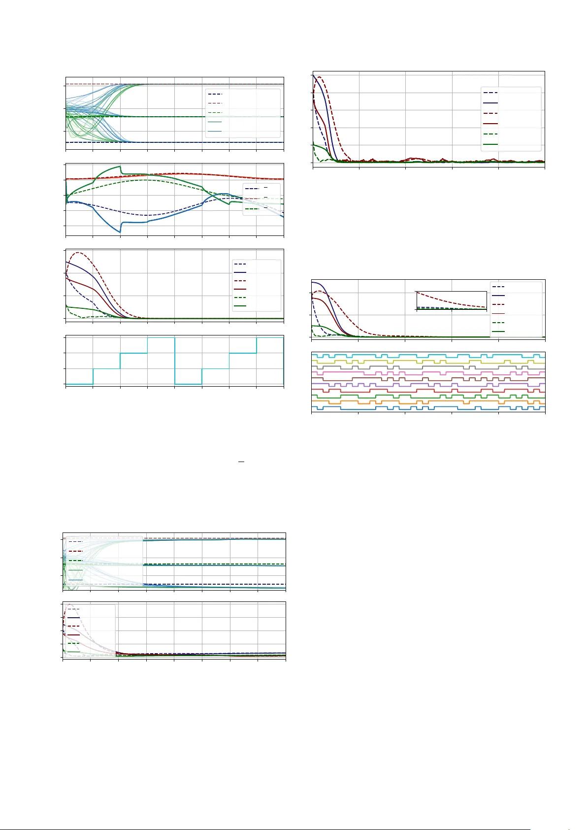
Hierarc hical parameter estimation for distributed net w ork ed systems: a dynamic consensus approac h Ariana R. Méndez-Castillo ∗ , ∗∗ Ro drigo Aldana-Lóp ez ∗∗ An tonio Ramírez-T reviño ∗ Rosario Aragues ∗∗ Da vid Gómez-Gutiérrez ∗∗∗ ∗ Dep artment of Ele ctric al Engine ering, Cinvestav-Guadalajar a, Jalisc o, 45019 Méxic o (e-mail: ariana.mendez@cinvestav.mx, antonio.r amir ezt@cinvestav.mx) ∗∗ Dep artment of Computing and Systems Enginering - I3A, University of Zar agoza, Zar agoza 50018 Esp aña (e-mail: r o drigo.aldana.lop ez@gmail.c om, r ar agues@unizar.es ) ∗∗∗ T e cnoló gic o Nacional de Méxic o, Instituto T e cnoló gic o José Mario Molina Pasquel y Henríquez, Cam. A r ener o 1101, 45019 Zap op an, Jalisc o, Mexic o. (e-mail: david.gomez.g@ie e e.or g) Abstract: This work introduces a nov el tw o-stage distributed framework to globally estimate constan t parameters in a netw orked system, separating shared information from lo cal estimation. The first stage uses dynamic a verage consensus to aggregate agen ts’ measurements in to surrogates of cen tralized data. Using these surrogates, the second stage implemen ts a lo cal estimator to determine the parameters. By designing an appropriate consensus gain, the p ersistence of excitation of the regressor matrix is ac hieved, and thus, exponential con vergence of a lo cal Gradient Estimator (GE) is guaranteed. The framework facilitates its extension to switc hed net w ork top ologies, quan tization, and the heterogeneous substitution of the GE with a Dynamic Regressor Extension and Mixing (DREM) estimator, which supp orts relaxed excitation requiremen ts. Keywor ds: Distributed estimation, Parameter estimation, Dynamic A v erage Consensus, Dynamic Regressor Extension and Mixing, Hierarchical estimation 1. INTR ODUCTION The fo cus of this w ork is on estimating unknown constan t parameters using linear regression data. This formulation naturally emerges in numerous applications, including adaptiv e con trol, co op erativ e rob otics, p o wer grids and sensor netw orks where reliable parameter iden tification is crucial for the stabilit y and performance of control strategies (Olfati-Sab er et al., 2007; Brouillon et al., 2024). In particular, linear regression mo dels app ear in rob ot manipulator control relating torques, join t co ordinates and the parameters of the rob ot (Gaz et al., 2019). ⋆ This work was supp orted in part by the Secretaría de Ciencia, Humanidades, T ecnología e Innov ación (SECIHTI), México, pre- viously administered by the Consejo Nacional de Humanidades, Ciencias y T ecnologías (CONAHCYT) with grant n umber 1229622, and in part by pro jects PID2021-124137OB-I00 and PID2024- 159279OB-I00 funded by MICIU/AEI/10.13039/501100011033 and by ERDF/EU, b y pro ject REMAIN S1/1.1/E0111 (Interreg Su- doe Programme, ERDF), and via pro ject DGA T45_23R (Go- bierno de Aragón). Grant reference BG24/00121 funded by MI- CIU/AEI/10.13039/501100011033. This w ork has been submitted for p ossible publication. Copyrigh t may b e transferred without no- tice, after whic h this v ersion may no longer be accessible. T w o arc hitectural categories can be distinguished: the c en- tr alize d one, where agents transmit their information to a cen tral unit that estimates the parameters, and the dis- tribute d one, where agen ts estimate the global parameters lo cally through collectiv e in teraction. In the latter setting, eac h agen t has access only to partial information. In the cen tralized case, different algorithms hav e b een prop osed as estimators. F or example, algorithms based on optimal filtering metho ds, such as the Kalman fil- ter in discrete time (Kalman, 1960; Maybeck, 1982) and the Kalman–Bucy filter in contin uous time (Golo v an and Mataso v, 2002) hav e b een used in the form of recursiv e least-squares iterations. They mo del the unkno wn param- eters as constan t states and th us, provide unbiased esti- mates with minim um v ariance under additiv e Gaussian measuremen t noise. How ever, the con vergence prop erties remain limited since the error cov ariance ev olv es according to a Riccati e quation guaranteeing asymptotic conv er- gence, but not exp onen tial (Zhang and Tian, 2016). T o solv e this inconv enience, algorithms relying on gradient- based methods w ere in tro duced. F or example, the Gra- dien t Estimator (GE) (Ioannou and Sun, 1996; Sastry and Bo dson, 2011) is widely used in b oth contin uous- and discrete-time designs, and is usually formulated for noiseless measurements. F or noisy measurements, the re- sulting estimation error can b e explicitly analyzed, and a closed-form expression for the cov ariance can b e derived (Moser et al., 2015). Exp onential conv ergence to the true parameters is guaranteed only when the p ersistence of excitation (PE) condition is main tained (Anderson, 2003). Ho wev er, PE is a sufficient but not necessary condition for correct parameter estimation. T o relax this requiremen t, the Dynamic Regressor Extension and Mixing (DREM) algorithm has been prop osed (Aranovskiy et al., 2016; Or- tega et al., 2021). DREM reformulates the original regres- sion into decoupled scalar equations, enabling parameter con vergence under excitation conditions w eaker than PE (Ortega et al., 2020). Unfortunately , centralized arc hitectures ha ve significan t limitations, such as high bandwidth requirements, the computational p ow er required by the central unit, and limited resilience to communication failures, among oth- ers (Kia et al., 2019). These limitations are exacerbated when the num b er of agents increases. T o face these chal- lenges, distributed estimators hav e b een introduced. Ex- amples include distributed extensions of Kalman filter based parameter estimators (Lendek et al., 2007; Ryu and Bac k, 2023), which only guaran tee asymptotic conv ergence under the same conditions as their cen tralized coun ter- parts. A widely studied alternativ e is the so called “ c on- sensus+ innovations ” framework (Kar and Moura, 2013; Lorenz-Mey er et al., 2025; Papusha et al., 2014). In this approac h, each agen t runs a tigh tly coupled gradient- based estimator with consensus enforceme n t (See Figure 1-T op). Con vergence relies on the notion of co op erativ e p ersistence of excitation (cPE) (Chen et al., 2014; Y an and Ishii, 2025; Zheng and W ang, 2016; Matveev et al., 2021), whic h ensures that the excitation condition is satisfied collectiv ely at the netw ork level. V ariants based on least mean squares consensus adaptiv e filters hav e also b een considered for different net work top ologies (Xie and Guo, 2018). A dra wback of this framework is its tightly cou- pled structure, where consensus and parameter estimation are closely in tertwined. In such approaches, conv ergence analyses dep end on joint Ly apunov argumen ts that simul- taneously treat b oth disagreemen t and estimation errors. Mo difying or replacing the underlying estimator requires substan tial changes to the en tire algorithm and a new con vergence analysis. Lik ewise, examining effects such as quan tization in communication is not straightforw ard. Lately , hierarc hical arc hitectures in multi-agen t settings ha ve been in vestigated for applications such as fault esti- mation (Liu et al., 2018), controller design (Cheng et al., 2023), and consensus algorithms (Chen et al., 2020), as they provide enhanced flexibility and heterogeneous lo cal strategies. Suc h arc hitectures also facilitate the in tegra- tion of consensus and estimation lay ers, since they can b e analyzed and implemen ted separately (Chen et al., 2020). In this context, hierarchical distributed parameter estimation schemes based on the DREM framework hav e b een proposed (Matveev et al., 2021; Y an and Ishii, 2025). Ho wev er, these approaches either require lo cal excitation conditions or fail to guarantee exp onential con vergence of the estimates. Consequently , no hierarchical metho d curren tly av ailable in the literature achiev es exp onential con vergence under the non-lo cal cPE condition. Motiv ated b y the previous discussion, the con tributions of this work are as follows. • W e in tro duce a hierarchical distributed parameter es- timation framework that decouples consensus from lo- cal estimation. A Dynamic A v erage Consensus (DA C) blo c k aggregates agents’ measurements into lo cal sur- rogates of the cen tralized regression, follo wed by a lo cal estimation blo ck that recov ers the unknown pa- rameters. Compared to consensus+inno v ations meth- o ds, this separation allo ws indep enden t analysis of consensus and estimation con vergence. • The prop osed framework is estimator agnostic. As a concrete instance, w e present the first distributed DREM-based estimator op erating under cPE, in con- trast to existing hierarchical approac hes which require lo cal excitation. • The results are further extended to switching com- m unication graphs and to scenarios with quantized information exchange. Notation: Let a, b ∈ R . W e write a ≥ b or a ≤ b to denote the usual order on R . Let R + denote the subspace of p ositive real num b ers. The flo or op erator ⌊•⌋ denotes the greatest integer less than or equal to its argument. The iden tity matrix of dimension n is denoted b y I n . Let 1 = [1 , . . . , 1] ⊤ ∈ R N . The i -th canonical v ector is denoted b y e i of appropriate dimension. The Kroneck er product is denoted by ⊗ . Let ∥ • ∥ denote the Euclidean norm for v ector inputs, and induced Euclidean norm for matrices. Let A b e a matrix. | A | represen ts the comp onent-wise absolute v alue. The largest eigen v alue of A is denoted by λ max ( A ) . The stacking op erator for matrices is denoted as col ( A i ) N i =1 = [ A ⊤ 1 . . . A ⊤ N ] ⊤ . The notation T r ( A ) represen ts the trace of the matrix A . The op erator vec ( A ) denotes the vectorization of the matrix A obtained by stac king its columns into a single v ector (Petersen et al., 2008, P age 60). Denote with ∥ • ∥ F = ∥ v ec ( • ) ∥ the F rob enius norm of a matrix. Let A ≻ B (resp. A ⪰ B ) b e the denote when the matrix A − B is p ositiv e definite (resp. p ositive semi-definite). 2. PR OBLEM ST A TEMENT AND PRELIMINARIES In this work, we consider a team of N monitoring agen ts in a netw orked system task ed to the estimation of a global v ector of unknown constant parameters θ ∈ R n . Eac h agen t is equipp ed with a lo cal sensor that takes measuremen ts of the form: y i ( t ) = C i ( t ) θ (1) where y i ( t ) ∈ R p i denotes the lo cal sensor output of the i th agent and C i ( t ) ∈ R p i × n is a time-v arying regressor matrix known by agent i ∈ { 1 , . . . , N } . W e fo cus on the non trivial case in whic h the information av ailable to each agen t is insufficient to identify θ on its o wn. In particular, for eac h agen t i , the lo cal regression matrix C i ( t ) may b e rank deficient ov er time, so that m ultiple parameter v alues are compatible with the lo cal measurements, thus requiring co op eration among agents to recov er θ . In this framework, agents share information through a comm unication netw ork mo deled as a connected, undi- rected graph G = ( V , E ) , with no de set V = { 1 , . . . , N } and edge set E ⊆ V × V . An edge ( i, j ) ∈ E indicates that agents i and j share information b etw een them. F or net work analysis purp oses, let A = [ a ij ] ∈ R N × N denote the adjacency matrix of G , with en tries a ij = a j i = 1 when ( i, j ) ∈ E and a ij = a j i = 0 otherwise. The degree matrix of G is denoted b y the diagonal matrix D ∈ N N × N with d ii = P j  = i a ij and the Laplacian matrix is defined as L = D − A . The set of neigh b ors of agent i is denoted as N i ⊆ V . The smallest nonzero eigenv alue λ G of L , called the algebraic connectivity , measures graph connectivity . The next subsection recalls the cen tralized parameter estimation version, where we highlight that the PE of a collectiv e regressor matrix is sufficien t to guarantee the exp onen tial con vergence of the gradient estimator to the true parameters. This is relev an t since a similar result will b e derived in our distributed prop osal. 2.1 Centr alize d estimation In the cen tralized estimation setting, there exists a cen tral station that collects all measurements y i ( t ) as y ( t ) = C ( t ) θ , with y ( t ) = col ( y i ( t )) N i =1 , C ( t ) = col ( C i ( t )) N i =1 (2) where C ( t ) ∈ R p × n and y ( t ) ∈ R p , with p = P N i =1 p i . Equipp ed with the pair y ( t ) , C ( t ) , the GE (Ioannou and Sun, 1996) can b e used to obtain an estimate ˆ θ c of the true parameter θ using an iteration in the form of the follo wing differen tial equation: ˙ ˆ θ c = Γ c C ( t ) ⊤ ( y ( t ) − C ( t ) ˆ θ c ) , (3) where the gain matrix Γ c ∈ R n × n , which satisfies 0 ≺ Γ c , determines the con vergence rate of the estimation dynamics and can b e tuned to accelerate con vergence. It can b e sho wn that (3) corresp onds to the gradient flow dynamics which minimizes the instan taneous estimation error: J c ( ˆ θ c ; t ) = 1 2 ∥ y ( t ) − C ( t ) ˆ θ c ∥ 2 . (4) T o study when (3) con verges to the true parameter θ , the follo wing standard definition is used: Definition 1. (Ioannou and Sun, 1996, A dapted from Def- inition 4.3.1) The matrix function F : R + → R m × n is said to comply with the Persistency of Excitation (PE) condition if there exists α, T > 0 such that for all t ≥ 0 : Z t + T t F ( τ ) ⊤ F ( τ ) d τ ⪰ α I n . (5) W e denote a function F that satisfies the PE condition as F ∈ PE ( α, T ) when the parameters α and T are relev an t and as F ∈ PE otherwise. The estimation error ˜ θ c = ˆ θ c − θ satisfies the following time-v arying dynamical system: ˙ ˜ θ c = − Γ c C ( t ) ⊤ C ( t ) ˜ θ c . (6) The next result establishes the con vergence of (6) to the origin when C ∈ PE. Pr op osition 1. (Ioannou and Sun, 1996, A dapted from Theorem 4.3.2) Let (6) b e the dynamics of the time- v arying error, with Γ c ≻ 0 and C ∈ PE, then, the origin of (6) is globally uniformly exp onentially stable. R emark 2. Proposition 1 sho ws that C ∈ PE is sufficien t for exp onen tial conv ergence of the centralized estimator, Fig. 1. Distributed parameter estimator framework. (T op) Sc heme of the consensus+inno v ations algorithm, im- plemen ted within the same blo c k. (Bottom) Scheme of the prop osed approach, where consensus and pa- rameter estimation are decoupled. while, in general, C i / ∈ PE for individual sensors. Thus C ∈ PE has b ecome a standard assumption on cen tralized and co op erativ e settings. This condition is referred to as c o op er ative p ersistency of excitation (cPE) (Chen et al., 2014; Y an and Ishii, 2025; Lorenz-Meyer et al., 2025). Requiring excitation at the lo cal lev el, is significan tly stronger and is only considered in sp ecific settings, such as (Matv eev et al., 2021). This motiv ates distributed mec ha- nisms that exploit co op eration to recov er cPE prop erties of the centralized mo del. 3. HIERAR CHICAL LOOSEL Y COUPLED ESTIMA TION The proposed hierarc hical framew ork equips eac h agen t with a Dynamic A verage Consensus (D AC) (Kia et al., 2019) blo ck and a lo cal parameter estimation blo ck (see Figure 1-Bottom). This structure decouples consensus dy- namics from estimator con vergence, av oiding the tight in terdep endence b et ween them, observed in existing ap- proac hes. As a consequence, the framework is estimator- agnostic b eing capable of supp orting differen t estimation sc hemes (e.g., GE, DREM), dep ending on the problem c haracteristics. In this section, we emplo y the GE scheme as a baseline, whereas the DREM estimator is introduced in Section 4. The first problem to tackle is the dimension mismatch among agents. F or this purp ose, the measurement in (1) is premultiplied as y ′ i ( t ) = C i ( t ) ⊤ y i ( t ) = C ′ i ( t ) θ , (7) where y ′ i ( t ) ∈ R n and C ′ i ( t ) = C i ( t ) ⊤ C i ( t ) . Now C ′ i ( t ) ∈ R n × n , and y ′ i ( t ) hav e the same dimension in every agent. The outputs y ′ i ( t ) and the regressor matrices C ′ i ( t ) of the agen ts are arranged in matrices y ′ ( t ) = col ( y ′ i ( t )) N i =1 C ′ ( t ) = col ( C ′ i ( t )) N i =1 (8) Equations y ′ ( t ) = C ′ ( t ) θ and y ( t ) = C ( t ) θ from (2) hav e the same solutions, as stated in the following prop osition. Pr op osition 3. Let y ( t ) , C ( t ) and y ′ ( t ) , C ′ ( t ) be defined as in (2) and (8), respectively . Then, an y θ ∈ R n is a solution y ′ ( t ) = C ′ ( t ) θ if and only if θ is a solution to y ( t ) = C ( t ) θ . All pro ofs are placed in App endix A. Next, w e sp ecify the consensus dynamics for the surrogate regressions C ′ i ( t ) together with the distributed estimation of the parameter vector θ . F or this purp ose, we emplo y (7) in place of (1), since, as sho wn in Prop osition 3 , b oth form ulations share the same solution set for θ . Based on this representation, we intr o duce the following algorithm, whic h in tegrates the consensus and distributed estimation la yers. Dynamic A v erage Consensus: ˙ X i ( t ) = k X j ∈N i  ˆ C i ( t ) − ˆ C j ( t )  (9a) ˙ x i ( t ) = k X j ∈N i  ˆ y i ( t ) − ˆ y j ( t )  (9b) Consensus output: ˆ C i ( t ) = C ′ i ( t ) − X i ( t ) , (9c) ˆ y i ( t ) = y ′ i ( t ) − x i ( t ) , (9d) Lo cal parameter estimation: ˙ ˆ θ i ( t ) = Γ i ˆ C i ( t ) ⊤  ˆ y i ( t ) − ˆ C i ( t ) ˆ θ i ( t )  (9e) where k > 0 , 0 ≺ Γ i ∈ R n × n are design parameters. The gains k and Γ i determine the conv ergence rates of the consensus and estimation dynamics resp ectively , and can b e tuned to accelerate conv ergence. As we show b elo w, an appropriate selection of k also ensures the PE prop ert y of the estimator regressor matrix. In addition, w e restrict the algorithm to the standard DA C initialization P N i =1 X i (0) = 0 , P N i =1 x i (0) = 0 with trivial setting X i (0) = 0 and x i (0) = 0 . R emark 4. The DA C blo ck in (9a)-(9d) allows agents to co operatively reconstruct global quantities of interest that w ould otherwise require centralized aggregation, pro duc- ing the surrogates ˆ C i ( t ) and ˆ y i ( t ) . The outputs of the D AC algorithm in (9c)–(9d) at each agent trac k the time- v arying av erage of the reference signals. Ideally , the DA C dynamics aim to enforce ˆ C i ( t ) = C ( t ) and ˆ y i ( t ) = y ( t ) , where C ( t ) = 1 N N X j =1 C ′ j ( t ) , y ( t ) = 1 N N X j =1 y ′ j ( t ) , (10) equally ˆ y i ( t ) = ˆ C i ( t ) θ (11) whic h motiv ates the structure of the second blo ck, namely the lo cal parameter estimator in (9e). The follo wing assumption is required to show the con ver- gence of (9), with similar analogs in the literature (Lorenz- Mey er et al., 2025): Assumption 1. There exists known β , γ > 0 with γ < ∞ , suc h that: sup τ ∈ [ t, ∞ ) ∥ ( H ⊗ I n ) ˙ C ′ ( τ ) ∥ ≤ γ , ∥ C ( t ) ∥ ≤ β for all t ≥ 0 , where H = I N − 11 ⊤ / N . R emark 5. Assumption 1 is a sufficient regularity condi- tion introduced to enable the analytical developmen t and con vergence guarantees of the prop osed estimators. It is satisfied b y a broad class of practically relev ant regressors, including those generated by b ounded linear systems and structured deterministic signals, as commonly assumed in adaptiv e and distributed estimation settings (Ioannou and Sun, 1996; P apusha et al., 2014; Matveev et al., 2021; Lorenz-Mey er et al., 2025). Consequently , the theoretical guaran tees derived in this work may not apply to all classes of regressors, and extending the analysis b eyond the considered class is left for future work. The following theorem shows that it is not necessary for the consensus outputs, ˆ C i ( t ) and ˆ y i ( t ) , to be exactly equal to (10). Instead, suitable design conditions ensure that the output ˆ θ i ( t ) of (9) conv erges to the true parameter θ . The or em 6. Supp ose Assumption 1 holds and let C ( t ) , defined in (2), b e PE ( α, T ) for some known α, T > 0 . If in Algorithm (9) the consensus gain k satisfies k > 2 nN 2 β γ T 2 λ G α 2 , (12) then the origin of the estimation error ˆ θ i ( t ) − θ is globally uniformly exp onentially stable for all i ∈ { 1 , . . . , N } . R emark 7. The low er b ound for feasible v alues of k in (12) can b e conserv atively estimated by o verestimating N and underestimating λ G . There exist distributed estimation approac hes (Montijano et al., 2011, 2017) in which each agen t indep endently estimates a v alue of λ G . When the maxim um num b er of no des N is known (for example, from netw ork capacit y sp ecified b y the comm unication proto col), the smallest p ossible λ G for a connected graph can b e used, which corresp onds to that of a linear graph, i.e. λ G = 2(1 − cos( π / N )) (De Abreu, 2007, T able 3.2). Since inter-agen t comm unication t ypically occurs o ver digital channels with finite data rates, we next accoun t for b ounded quan tization effects in the consensus la y er. In particular, w e replace the DA C blo c k in (9a),(9b) of Algorithm (9) by the following quan tized version: Quan tized Dynamic A v erage Consensus: ˙ X i ( t ) = k X j ∈N i  Q ( ˆ C i ( t )) − Q ( ˆ C j ( t ))  , (13a) ˙ x i ( t ) = k X j ∈N i  Q ( ˆ y i ( t )) − Q ( ˆ y j ( t ))  , (13b) while keeping the consensus outputs (9c), (9d) and the lo- cal parameter estimator (9e) unc hanged. The quan tization op erator Q ( • ) is defined comp onent wise as Q ( s ) = ε  s/ε  , and is applied element-wise when acting on vectors or matrices, where ε > 0 denotes the size of the quan tization step. Cor ol lary 8. Let ε > 0 b e the size of the quantization step. Assume that C ( t ) in (2) is PE ( α, T ) for some known α, T > 0 , and Assumption 1 holds . Consider Algorithm (9) with the quantized consensus dynamics (13a), (13b) and the lo cal estimator (9e). If k and ε satisfy α 2 T N 2 > 2 β T nγ k λ G + n 2 √ N λ max ( L ) λ G ε ! , then there exists T q > 0 suc h that the estimation error complies ∥ ˆ θ i ( t ) − θ ∥ ≤ B ( ε ) for all t ≥ T q , where B ( • ) is con tinuous, strictly increasing and comply B (0) = 0 . Corollary 8 can b e extended to a switching netw ork top ology G σ ( t ) with a switc hing signal σ ( t ) ∈ { 1 , . . . , q } , selecting among a family of connected undirected graphs {G 1 , . . . , G q } , by replacing Dynamic A verage Consensus blo c k in (13a) and (13b) with: Switc hed Dynamic A v erage Consensus: ˙ X i ( t ) = k X j ∈N i,σ ( t )  Q ( ˆ C i ( t )) − Q ( ˆ C j ( t ))  , (14a) ˙ x i ( t ) = k X j ∈N i,σ ( t )  Q ( ˆ y i ( t )) − Q ( ˆ y j ( t ))  , (14b) where N i,σ ( t ) is the neighbor set of agent i . Cor ol lary 9. Under the Assumptions of Corollary 8, let G σ ( t ) b e a switc hing netw ork top ology with G ℓ , ℓ = 1 , . . . , q a connected undirected graph and the switching signal σ ( t ) satisfying a minimum dwell-time. Moreov er, let k and ε satisfy α 2 T N 2 > 2 β T nγ k λ G ,m + n 2 √ N λ G ,M λ G ,m ε ! , where λ G ,M = max ℓ ∈{ 1 ,...q } λ max ( L ℓ ) and λ G ,m = min ℓ ∈{ 1 ,...q } λ ℓ and λ ℓ , L ℓ are the algebraic connectivit y and Laplacian of G ℓ resp ectiv ely . Then, under algorithm (14a), (14b) together with (9c), (9d) and (9e), there exists T q > 0 such that the estimation error complies ∥ ˆ θ i ( t ) − θ ∥ ≤ B ( ε ) for all t ≥ T q , where B ( • ) is contin uous strictly increasing with B (0) = 0 . As shown in Appendix A.2, the proof of Corollary 8 is based on a graph-indep endent Ly apunov function. Thus, the pro of of Corollary 9 follo ws from a common Lyapuno v function argument with the dwell-time condition ensuring the w ell-p osedness of the resulting dynamics (Liberzon, 2003). 4. DISTRIBUTED DREM The DREM approach requires a weak er PE condition to guaran tee the conv ergence of the estimated parameters. Therefore, it can b e used as an alternative to the GE and ma y remain effective even if the GE fails. The DREM (Aranovskiy et al., 2016) prop oses applying linear, L ∞ -stable op erators H i to the linear regression equation. In particular, for example, exp onen tially stable linear time-inv ariant filters of the form H j ( • ) = α j p + β j ( • ) (15) where p = d dt , and α j  = 0 , β j > 0 can b e used. These filters introduce additional information, generally seeking to hav e a square matrix from whic h a scalar equation for eac h parameter is obtained after multiplication with its adjugate. In our case, we prop ose in tro ducing linear, L ∞ -stable op erators on ˆ C i ( t ) and ˆ y i ( t ) , presented in equations (9c)– (9d), stacking the result in matrices C f i ( t ) and y f i ( t ) , resp ectiv ely , until det( C f i ( t ) ⊤ C f i ( t )) / ∈ L 2 . Th us, the GE blo c k in (9e) is replaced b y a DREM estimator as follows: Lo cal parameter estimation: C f i ( t ) = [ ˆ C i ( t ) ⊤ H 1 [ ˆ C i ( t )] ⊤ . . . H r [ ˆ C i ( t )] ⊤ ] ⊤ (16a) y f i ( t ) = [ ˆ y i ( t ) ⊤ H 1 [ ˆ y i ( t )] ⊤ . . . H r [ ˆ y i ( t )] ⊤ ] ⊤ (16b) ϕ i ( t ) = det ( C f i ( t ) ⊤ C f i ( t )) (16c) Y i ( t ) = adj ( C f i ( t ) ⊤ C f i ( t ))( C f i ( t ) ⊤ y f i ( t )) (16d) ˙ ˆ θ i ( t ) = Γ i ϕ i ( t )  Y i ( t ) − ϕ i ( t ) ˆ θ i ( t )  . (16e) where Γ i ≻ 0 is a diagonal matrix and a design parameter and H j : L ∞ → L ∞ is a linear, L ∞ -stable op erator with j ∈ { 1 , . . . , r } . Cor ol lary 10. Let (9c), (9d) b e consensus outputs and let C f i ( t ) b e defined in (16a). If the num ber r of op erators H j mak es ϕ i ( t ) / ∈ L 2 , then ˆ θ i ( t ) in (16e) conv erges exp onen tially to θ . Algorithm (16) is based on introducing the necessary n um- b er of operators H j that allo w us to expand the infor- mation av ailable to each agent. Ho wev er, the consensus output could fulfill condition (A.9) on its o wn, so it would not b e necessary to introduce op erators, i.e., r = 0 . F urthermore, when the matrix ˆ C i ( t ) resulting from the consensus in (9c) is PE or ϕ i = det( ˆ C i ( t )) satisfies condition (A.9), a simpler version of the lo cal DREM- based parameter estimator is given b y Lo cal parameter estimation: ϕ i ( t ) = det  ˆ C i ( t )  , (17a) Y i ( t ) = adj  ˆ C i ( t )  ˆ y i ( t ) , (17b) ˙ ˆ θ i ( t ) = Γ i ϕ i ( t )  Y i ( t ) − ϕ i ( t ) ˆ θ i ( t )  . (17c) Cor ol lary 11. Let ˆ C i ( t ) and ˆ y i ( t ) b e the consensus out- puts defined in (9c)–(9d). If ˆ C i ( t ) is PE or det( ˆ C i ( t )) / ∈ L 2 , then ˆ θ i in (17c) conv erges exp onentially to θ . 5. DISCUSSION Based on the obtained results, we emphasize that the pro- p osed architecture (see b ottom Figure 1) for distributed parameter estimation is b oth flexible and v ersatile, as it enables the decoupling of the consensus analysis from the parameter estimation pro cess. The architecture is com- p osed of tw o blo c ks: a consensus mo dule and a parameter estimation mo dule. In the consensus stage, one works with surrogate versions of the regressor matrices instead of the original ones. A key adv an tage of this approach is that the surrogate signals ˆ C i ( t ) exhibit lo cal PE even in cases where the original regressor matrices do not ha v e this prop erty . This is guaranteed b y selecting the gain according to a computable b ound (see Theorem 6). This allo ws us to formulate a new regressor equation that relies on the surrogates in place of the original regressor matrices in (11) (see Lemma 14). Because the surrogates possess the prop ert y of p ersistent excitation, the parameter estimation pro cess is ensured to conv erge exp onen tially to the true 1 2 3 4 5 6 7 8 9 10 (a) σ = 1 1 2 3 4 5 6 7 8 9 10 (b) σ = 2 10 2 3 4 5 6 7 8 9 1 (c) σ = 3 10 2 3 4 5 6 7 8 9 1 (d) σ = 4 Fig. 2. Collection of comm unication topologies G σ used for the switc hed dynamic netw ork in the n umerical example. parameter v alues. That is to sa y , the consensus mo dule do es not act directly on the parameter estimates, but rather on the regression data. By exploiting the separa- tion betw een analyses, the arc hitecture b ecomes mo dular, allo wing different algorithms to b e applied at eac h stage. This flexibility enables it to capture v arious phenomena found in real-world problems. F or instance, during the consensus phase, it is p ossible to incorp orate effects like data quantization/rounding and switc hing comm unication graphs, while still demonstrating that the surrogates retain the p ersisten t excitation prop erty . F urthermore, in the estimation phase, we demonstrated that both gradien t- descen t and DREM-based estimation metho ds can be em- plo yed, and in eac h case the true parameter v alues are successfully recov ered. 6. NUMERICAL EXAMPLES W e consider N = 10 agents connected b y a collection of undirected graphs G σ giv en in Figures 2a-2d. The switc hed net work ev olves according to a switching signal σ ( t ) ∈ { 1 , 2 , 3 , 4 } . F or eac h agent i , the measurements are giv en by y i ( t ) = C i ( t ) θ with n = 3 , where C i ( t ) ∈ R 1 × n consists of terms of the form A + B sin( ω t ) + D cos( ωt ) . The parameters ω , A, B , and D are sampled from uniform distributions, with A, B , D sampled ov er [0 , 20] and ω sampled ov er [0 , 3] . Based on these v alues, sim ulations yield γ = 8 . 3966 , β = 20 . 769 , α = 51 . 326 , T = 0 . 16 , and min σ ∈{ 1 , 2 , 3 , 4 } λ σ = 0 . 367 . Using these parameters, the consensus gain must satisfy k > 2 . 778 . In the simulations, w e select k = 2 . 806 . The examples in this section illustrate that b oth esti- mation approaches, distributed GE and DREM, achiev e go od p erformance. In all figures, blue corresp onds to θ 1 , red to θ 2 , and green to θ 3 . In the parameter estimation graphs, the gradient-based approach is depicted in green, while DREM is depicted in blue. Let ˜ θ i,µ represen t the estimation error of agen t i with resp ect to θ µ , µ = 1 , . . . , n . In the estimation error plots, w e group all errors related to θ µ in to the vector e µ = [ ˜ θ 1 ,µ , . . . , ˜ θ N ,µ ] . Figure 3 shows the simulation results with a quan tization step size of zero. The upp er graph shows the estimate for each agent’s parameter estimate, while the dashed lines indicate the actual parameter v alues to b e identified. The GE is shown in green and the DREM estimator in blue. In b oth cases, the estimates conv erge exp onen tially to the true v alues. The upp er-middle graph sho ws the consensus output, where the dotted line represents the a verage v alue y ( t ) , in (10), and the solid lines represent eac h consensus output ˆ y i ( t ) in (9d). The lo wer-middle plot presen ts the estimation error ∥ e i ∥ for i ∈ { 1 , 2 , 3 } . The dashed line corresp onds to the GE error, while the solid line represents the DREM estimator error. In b oth cases, the errors conv erge exp onentially to zero. The graphs switc h according to the signal σ ( t ) , sho wn in the low er panel. In the next exp erimen t, we use a quantization step of ε = 0 . 036 , in accordance with the assumptions of Corollary 9, and keep the consensus gain v alue unchanged. The result is shown in Figure 4. The upp er graph displays the estimated parameters, rev ealing a small offset. The lo wer graph shows that, due to the quan tization error, the estimation error does not exactly con v erge to zero, in agreement with Corollary 9. T o further illustrate the capabilities of the prop osed ap- proac h, we examine the case in whic h noise is added to sen- sor measuremen ts. Sp ecifically , we take y i ( t ) = C i ( t ) θ + η i ( t ) , where w e sample η i ( t ) as zero-mean Gaussian noise with a standard deviation e qual to 0 . 2 for each simulation step. As shown in Figure 5, the parameter estimates are affected by noise. Nevertheless, the estimation error still con verges exp onentially to a neigh b orho o d of the origin. Because the noise scales with the consensus gain, increas- ing this gain results in a p oorer estimate. This outcome suggests that the parameter can b e reco vered with reason- able accuracy in presence of noise. Finally , we consider the scenario in which information is lost during communication b et ween agen ts. The sim ulation results are presented in Figure 6. In the upp er graph, the estimation error decreases at an exp onential rate. The low er graph illustrates the information flow by each agen t, arranged from b ottom to top. A high level represent p eriods when the agent is sending information, whereas lo w lev el indicate that the agen t is not transmitting. 7. CONCLUSION This w ork presented a hierarchical distributed estimation framew ork that decouples the D A C algorithm from the parameter estimation. As a result, b y calculating an appro- priate consensus a regression matrix can be obtained that satisfies the PE condition, even when the communication top ology switches ov er time. Under this condition, exp o- nen tial conv ergence is ensured for tw o distinct parameter estimation metho ds: GE and DREM, enabling flexibility − 5 0 5 ˆ θ i θ 1 θ 2 θ 3 Distributed GE Distributed DREM − 150 − 100 − 50 0 50 ˆ y i ( t ) y 1 ( t ) y 2 ( t ) y 3 ( t ) 0 10 20 30 k e 1 k GE k e 1 k DREM k e 2 k GE k e 2 k DREM k e 3 k GE k e 3 k DREM 0 . 0 0 . 5 1 . 0 1 . 5 2 . 0 2 . 5 3 . 0 3 . 5 4 . 0 Time 1 2 3 4 σ ( t ) Fig. 3. Sim ulation results. Colors are related to the param- eters θ 1 (blue), θ 2 (red), and θ 3 (green). (T op) P aram- eters estimation ˆ θ i,µ , for eac h agent for GE (green) and DREM (blue); dashed lines show θ . (T op-middle) Dashed line represents the av erage v alue ( y ( t ) ), while solid lines represent the individual consensus outputs ˆ y i ( t ) . (Low-middle) Magnitude of the estimation error e i , dashed for GE and solid for DREM. (Bottom) The switc hing signal σ ( t ) . − 5 0 5 ˆ θ i θ 1 θ 2 θ 3 Distributed GE Distributed DREM 0 1 2 3 4 5 6 7 8 Time 0 10 20 30 40 k e 1 k GE k e 1 k DREM k e 2 k GE k e 2 k DREM k e 3 k GE k e 3 k DREM Fig. 4. Simulation results using quantization. Colors are re- lated to the parameters θ 1 (blue), θ 2 (red) θ 3 (green). (T op) P arameter estimation for eac h agent for GE (green) and DREM (blue); dashed lines sho w θ . (Bot- tom) Magnitude of estimation error e i , dashed lines for GE and solid for DREM. 0 2 4 6 8 10 Time 0 5 10 15 20 25 k e 1 k GE k e 1 k DREM k e 2 k GE k e 2 k DREM k e 3 k GE k e 3 k DREM Fig. 5. Sim ulation results with additive Gaussian sensor noise mo deled as y i ( t ) = C i ( t ) θ + η i ( t ) , where η i ( t ) is Gaussian noise with mean 0 and standard deviation equal to 0 . 2 . Estimation error magnitudes e 1 (blue), e 2 (red), and e 3 (green) are sho wn; dotted lines indicate GE and solid lines DREM. 0 10 20 k e 1 k GE k e 1 k DREM k e 2 k GE k e 2 k DREM k e 3 k GE k e 3 k DREM 0 2 4 6 8 10 Time 9 . 0 9 . 5 10 . 0 0 . 000 0 . 002 Fig. 6. Sim ulation results with communication loss. (T op) Magnitude of estimation errors e 1 ( t ) (blue), e 2 (red), and e 3 (green), where dotted lines correspond to GE and solid lines to DREM. (Bottom) Information transmitted by eac h agent. High level indicates that information is being sen t, while the low level indicates no transmission. in the c hoice of estimator while preserving the adv an- tages of each. The framework further allows for quantized comm unication b etw een agents, yielding an estimation error that remains ultimately b ounded, with its magni- tude dictated by the chosen quan tization step. All results are v alidated through a Lyapuno v-function-based analysis, whic h guarantees global and exp onential stabilit y . The results are confirmed by the sim ulations. F or both GE and DREM, the estimation error exhibits exp onen tial conv er- gence. This b ehavior holds across all analyzed scenarios and aligns with the theoretical predictions. F urthermore, ev en in the presence of comm unication losses and sen- sor measuremen t noise, the estimators exhibit satisfactory p erformance, illustrating the practical robustness of the prop osed framew ork. As future w ork, we aim to inv estigate adaptiv e gain tuning laws to ov ercome the limitation of kno wing the low er b ound for admissible consensus gain in adv ance. Moreo ver, the impact of comm unication losses and measurement noise is yet to b e analyzed formally . In addition, the prop osed framew ork may b e extended to non- linear measurement mo dels and even t-triggered proto cols. App endix A. PROOFS A.1 Pr o of of Pr op osition 3 Set W = { θ ∈ R n : y ( t ) = C ( t ) θ } and W ′ = { θ ∈ R n : y ′ ( t ) = C ′ ( t ) θ } . T ake an y θ ∈ W ′ . Then y ′ ( t ) = C ′ ( t ) θ = C ( t ) ⊤ C ( t ) θ . Since y ′ ( t ) = C ( t ) ⊤ y ( t ) , we obtain C ( t ) ⊤ ( y ( t ) − C ( t ) θ ) = 0 . Hence w := y ( t ) − C ( t ) θ ∈ Ker ( C ( t ) ⊤ ) . Therefore, w ∈ Im ( C ( t )) ⊥ b y the identit y Ker ( C ( t ) ⊤ ) = Im ( C ( t )) ⊥ , where Im ( • ) ⊥ denotes the orthogonal comple- men t of Im ( • ) (Horn and Johnson, 1990, Page 16). On the other hand, since y ( t ) ∈ Im ( C ( t )) , we conclude that w ∈ Im ( C ( t )) . The only v ector b elonging simultaneously to Im ( C ( t )) and its orthogonal complement is w = 0 . Henceforth y ( t ) = C ( t ) θ , implying θ ∈ W . This shows W ′ ⊆ W . Conv ersely , if θ ∈ W , then pre-multiplying y ( t ) = C ( t ) θ b y C ( t ) ⊤ giv es y ′ ( t ) = C ( t ) ⊤ y ( t ) = C ( t ) ⊤ C ( t ) θ = C ′ ( t ) θ , so θ ∈ W ′ , i.e. W ⊆ W ′ . Therefore, W = W ′ . A.2 A uxiliary lemmas for The or em 6 T o facilitate the pro of of Theorem 6, the following tec hni- cal lemmas are in tro duced. L emma 12. Let C ( t ) = C ⊤ ( t ) C ( t ) / N . If C ( t ) in (2) is PE ( α, T ) , for some α, T > 0 , then C ( t ) 2 ∈ PE ( α 2 T N 2 , T ) . Pro of. By definition C ( t ) = 1 N C ( t ) ⊤ C ( t ) , then R t + T t C ( τ ) d τ = 1 N R t + T t C ( τ ) ⊤ C ( τ ) d τ ⪰ α N I n . Hence- forth, for any v ∈ R n with ∥ v ∥ = 1 it follows that:  α N  2 ≤ " v ⊤ Z t + T t C ( τ ) d τ ! v # 2 = " Z t + T t v ⊤ C ( τ ) v d τ # 2 ≤ T Z t + T t ( v ⊤ C ( τ ) v ) 2 d τ where we used the Cauch y-Sch w arz inequalit y with g ( τ ) = 1 and h ( τ ) = v ⊤ C ( τ ) v . Moreov er, using again the Cauc hy-Sc hw arz inequality: ( v ⊤ C ( τ ) v ) 2 ≤ ∥ v ∥ 2 ∥ C ( τ ) v ∥ 2 = ( C ( τ ) v ) ⊤ ( C ( τ ) v ) = v ⊤ C ⊤ ( τ ) C ( τ ) v = v ⊤ C ( τ ) 2 v Therefore 1 T  α N  2 ≤ R t + T t v ⊤ C ( τ ) 2 v d τ = v ⊤ R t + T t C ( τ ) 2 d τ v . Recall that the previous inequalit y holds for all unit vectors v ∈ R n . Then, 1 T  α N  2 I n ⪯ R t + T t C ( τ ) 2 d τ which completes the pro of. L emma 13. Let the consensus error at agen t i b e denoted as ˜ C i ( t ) = ˆ C i ( t ) − C ( t ) . If the Assumption 1 holds then there exists a finite time T ˜ C ( ˜ C i (0)) > 0 suc h that ∥ ˜ C i ( t ) ∥ ≤ nγ k λ G ∀ t ≥ T ˜ C ( ˜ C i (0)) . Pro of. Stacking the local v ariables of all agen ts as X ( t ) = col ( X i ( t )) N i =1 , ˆ C ( t ) = col ( ˆ C i ( t )) N i =1 and considering the a verage defined in (10), w e rewrite as C ( t ) = 1 N ( 1 ⊤ ⊗ I n ) C ′ ( t ) . Defining the stack ed consensus error by ˜ C ( t ) = col ( ˜ C i ( t )) N i =1 = ˆ C ( t ) − ( 1 ⊗ I n ) C ( t ) , where ˜ C i ( t ) = ( e ⊤ i ⊗ I n ) ˜ C ( t ) is the error of agent i . The writing of (9a)–(9c) in v ector form leads to: ˙ X ( t ) = k ( L ⊗ I n ) ˆ C ( t ) , ˆ C ( t ) = C ′ ( t ) − X ( t ) . (A.1) Therefore, ˙ ˜ C ( t ) = ˙ ˆ C ( t ) − ( 1 ⊗ I n ) ˙ C ( t ) ˙ ˜ C ( t ) = ˙ C ′ ( t ) − ˙ X ( t ) − ( 1 ⊗ I n )  1 N ( 1 ⊤ ⊗ I n ) ˙ C ′ ( t )  = − k ( L ⊗ I n ) ˜ C ( t ) + ( H ⊗ I n ) ˙ C ′ ( t ) , where H = I N − 11 ⊤ / N . A quadratic function is commonly employ ed as the Lya- puno v candidate. Consistent with this, we employ the v ectorization of ˜ C ( t ) and define V ( ˜ C ) = vec ( ˜ C ) ⊤ v ec ( ˜ C ) . By exploiting properties of the v ectorization operator, this can b e rewritten as V ( ˜ C ) = T r ( ˜ C ⊤ ˜ C ) , and its deriv ativ e is giv en by ˙ V ( ˜ C ( t )) = 2 T r ( ˜ C ( t ) ⊤ ˙ ˜ C ( t )) . Using the inequal- ities | T r ( AB ) | ≤ ∥ A ∥ F ∥ B ∥ F and || A || F ≤ p rank ( A ) ∥ A ∥ (P etersen et al., 2008, P ages 61-62). ˙ V ( ˜ C ( t )) = 2 T r  − k ˜ C ( t ) ⊤ ( L ⊗ I n ) ˜ C ( t ) + ˜ C ( t ) ⊤ ( H ⊗ I n ) ˙ C ′ ( t )  ≤ − 2 kλ G ∥ ˜ C ( t ) ∥ 2 + 2 n ∥ ˜ C ( t ) ∥∥ ( H ⊗ I n ) ˙ C ′ ( t ) ∥ = − 2 ∥ ˜ C ( t ) ∥  k λ G ∥ ˜ C ( t ) ∥ − n ∥ ( H ⊗ I n ) ˙ C ′ ( t ) ∥  Th us, ˙ V ( ˜ C ( t )) < 0 in the region where: ∥ ˜ C ( t ) ∥ ≥ n ∥ ( H ⊗ I n ) ˙ C ′ ( t ) ∥ k λ G . Hence, tra jectories of ˜ C ( t ) will conv erge in finite time T ˜ C ( ˜ C i (0)) > 0 to the region in which the following condition remains inv ariant: ∥ ˜ C ( t ) ∥ ≤ n ∥ ( H ⊗ I n ) ˙ C ′ ( t ) ∥ k λ G ≤ n sup τ ∈ [ t, ∞ ) ∥ ( H ⊗ I n ) ˙ C ′ ( τ ) ∥ k λ G . Due to Assumption 1 ∥ ˜ C ( t ) ∥ ≤ nγ k λ G , completing the pro of. L emma 14. Consider (9a)–(9d) driven by the lo cal surro- gate signals (7). Assume the standard DA C initialization X i (0) = 0 and x i (0) = 0 for all i ∈ { 1 , . . . , N } . Then, for all t ≥ 0 and all i ∈ { 1 , . . . , N } , ˆ y i ( t ) = ˆ C i ( t ) θ . Pro of. Define r i ( t ) = ˆ y i ( t ) − ˆ C i ( t ) θ . Using (9c)–(9d) and (7), we obtain r i ( t ) =  y ′ i ( t ) − x i ( t )  −  C ′ i ( t ) − X i ( t )  θ = − x i ( t )+ X i ( t ) θ . Differen tiating and using (9a)–(9b) yields ˙ r i ( t ) = − ˙ x i ( t ) + ˙ X i ( t ) θ = − k X j ∈N i  ˆ y i ( t ) − ˆ y j ( t )  + k X j ∈N i  ˆ C i ( t ) − ˆ C j ( t )  θ = − k X j ∈N i  r i ( t ) − r j ( t )  . Equiv alen tly , in stac ked form r ( t ) = col( r i ( t )) N i =1 satisfies ˙ r ( t ) = − k ( L ⊗ I n ) r ( t ) . Moreo ver, r (0) = 0 since X i (0) = 0 and x i (0) = 0 for all i . Hence, r ( t ) = 0 for all t ≥ 0 , whic h implies ˆ y i ( t ) = ˆ C i ( t ) θ for all t ≥ 0 . A.3 Pr o of of The or em 6 Giv en (9e), define the estimate error of agent i as ˜ θ i = ˆ θ i − θ . By Lemma 14, under the standard DA C initialization X i (0) = 0 and x i (0) = 0 , the consensus outputs satisfy ˆ y i ( t ) = ˆ C i ( t ) θ for all t ≥ 0 . Moreov er, since C ′ i ( t ) = C i ( t ) ⊤ C i ( t ) is symmetric and X i (0) = 0 is symmetric, the DA C dynamics preserve symmetry , and thus ˆ C i ( t ) is symmetric for all t ≥ 0 . Substituting into (9e) yields ˙ ˆ θ i ( t ) = Γ i ˆ C i ( t ) ⊤  ˆ y i ( t ) − ˆ C i ( t ) ˆ θ i ( t )  = Γ i ˆ C i ( t )  ˆ C i ( t ) θ − ˆ C i ( t ) ˆ θ i ( t )  = Γ i ˆ C i ( t ) 2  θ − ˆ θ i ( t )  . whic h giv es the error dynamics ˙ ˜ θ i ( t ) = − Γ i ˆ C i ( t ) 2 ˜ θ i ( t ) . (A.2) As indicated in Proposition 1, if ˆ C i ( t ) is PE, then ˜ θ i → 0 , consequen tly ˆ θ i → θ . Therefore, the rest of the pro of sho ws that ˆ C i ( t ) is PE, provided the consensus gains complies with (12). The consensus output at agen t i is defined as ˆ C i ( t ) = ˜ C i ( t ) + C ( t ) . The integral to b e ev aluated is: Z t + T t ˆ C i ( τ ) 2 d τ = Z t + T t  C ( τ ) + ˜ C i ( τ )  2 d τ = Z t + T t  C ( τ ) 2 + ˜ C i ( τ ) 2 + C ( τ ) ˜ C i ( τ ) + ˜ C i ( τ ) C ( τ )  d τ considering R t + T t ˜ C i ( τ ) 2 d τ ⪰ 0 and according to Lemma 12 it follows that R t + T t  C ( τ )  2 d τ ⪰ α 2 T N 2 I n . W e use the Euclidean norm on the non-square terms of the integral. ∥ C ( t ) ˜ C i ( t ) + ˜ C i ( t ) C ( t ) ∥ ≤ ∥ C ( t ) ˜ C i ( t ) ∥ + ∥ ˜ C i ( t ) C ( t ) ∥ ≤ 2 ∥ C ( t ) ∥∥ ˜ C i ( t ) ∥ (A.3) By assumption ∥ C ( t ) ∥ ≤ β and according to Lemma 13 ∥ ˜ C i ( t ) ∥ ≤ nγ λ G k then 2 ∥ C ( t ) ∥∥ ˜ C i ( t ) ∥ ≤ 2 β nγ λ G k . Therefore Z t + T t ( ˆ C i ( τ )) 2 d τ ⪰ Z t + T t  C 2 ( τ ) − 2 β  nγ λ G k  I n  d τ ⪰  α 2 T N 2 − 2 β  nγ λ G k  T  I n = φ I n Consequen tly , b y assumption k > 2 nβ γ T 2 N 2 λ G α 2 making φ > 0 . As a result, ˆ C i ( t ) is PE, whic h completes the pro of. A.4 Pr o of of Cor ol lary 8 F or each agent i , Q ( ˆ C i ( t )) = ˆ C i ( t ) + ε i ( t ) , Q ( ˆ y i ( t )) = ˆ y i ( t ) + ε y i ( t ) , with ∥ ε i ( t ) ∥ ≤ n ε, ∥ ε y i ( t ) ∥ ≤ √ n ε, ∀ t ≥ 0 . Stac king ε i as ε = col ( ε i ) N i =1 , with ∥ ε ( t ) ∥ ≤ n √ N ε and ε y = col ( ε y i ) N i =1 with ∥ ε y ( t ) ∥ ≤ √ nN ε, ∀ t ≥ 0 , the vector form of (13a)–(9d) yields ˙ ˜ C ( t ) = − k ( L ⊗ I n ) ˜ C ( t ) + ( H ⊗ I n ) ˙ C ′ ( t ) − k ( L ⊗ I n ) ε ( t ) , where ˜ C ( t ) = ˆ C ( t ) − ( 1 ⊗ I n ) C ( t ) and H = I N − 11 ⊤ / N . Using the same Lyapuno v function V ( ˜ C ) = T r( ˜ C ⊤ ˜ C ) as in Lemma 13, the additional term − k ( L ⊗ I n ) ε ( t ) acts as a b ounded disturbance, which implies that ˜ C ( t ) is uniformly ultimately b ounded. In particular, there exists a finite time T q ( ˜ C i (0)) > 0 suc h that, for all t ≥ T q ( ˜ C i (0)) and all i , ∥ ˜ C i ( t ) ∥ ≤ nγ k λ G + εn 2 √ N λ max ( L ) λ G =: b ( ε ) . (A.4) Therefore, for t ≥ T q ( ˜ C i (0)) , ˆ C i ( t ) = C ( t ) + ˜ C i ( t ) is a b ounded p erturbation of C ( t ) . Since C ( t ) 2 ∈ PE  α 2 T N 2 , T  b y Lemma 12, the same in tegral lo w er-b ound argument used in the pro of of Theorem 6 gives, for all t ≥ T q ( ˜ C i (0)) , Z t + T t ˆ C i ( τ ) 2 d τ ⪰ φ I n , (A.5) where φ = α 2 T N 2 − 2 β T nγ k λ G + εn 2 √ N λ max ( L ) λ G ! . Under the condition stated in Corollary 8, φ is strictly p ositiv e, and hence ˆ C i ( t ) is p ersistently exciting. Due to quantization, the exact relation ˆ y i ( t ) = ˆ C i ( t ) θ no longer holds. In fact, the consensus relation yields ˆ y i ( t ) = ˆ C i ( t ) θ + r i ( t ) . Similarly to the pro of of Lemma 14, using (9c)–(9d) r i ( t ) = X i ( t ) θ − x i ( t ) , differen tiating and using (13a)–(13b) ˙ r i ( t ) = − ˙ x i ( t ) + ˙ X i ( t ) θ = − k X j ∈N i  Q ( ˆ y i ( t )) − Q ( ˆ y j ( t ))  + k X j ∈N i  Q ( ˆ C i ( t )) − Q ( ˆ C j ( t ))  θ , stac king r ( t ) = col ( r i ( t )) N i =1 , the vector form is ˙ r ( t ) = k ( L ⊗ I n )  ˆ C ( t ) θ − ˆ y ( t ) − ε ( t ) θ + ε y ( t )  = − k ( L ⊗ I n ) r ( t ) + k ( L ⊗ I n )( ε y ( t ) − ε ( t )) Define a candidate Ly apunov function as V ( r ) = 1 2 r ( t ) ⊤ r ( t ) , with ˙ V ( r ( t )) = − k r ( t ) ⊤ ( L ⊗ I n )  r ( t ) − ε y ( t ) + ε ( t ) θ  . Since r (0) = 0 and ( 1 ⊤ ⊗ I n ) ˙ r ( t ) = 0 , then ( 1 ⊤ ⊗ I n ) r ( t ) = 0 for all t , and therefore we obtain k r ( t ) ⊤ ( L ⊗ I n ) r ( t ) ≥ kλ G ∥ r ( t ) ∥ 2 . Hence ˙ V ( r ( t )) ≤ − k ∥ r ( t ) ∥ 2 λ G + k ∥ r ( t ) ∥ λ max ( L )  ∥ ε y ( t ) ∥ + ∥ ε ∥∥ θ ∥  ≤ − k ∥ r ( t ) ∥ 2 λ G + k ∥ r ( t ) ∥ λ max ( L )  √ nN ε + n √ N ε ∥ θ ∥  . Substituting 2 V ( r ( t )) = ∥ r ( t ) ∥ 2 , ˙ V ( r ( t )) ≤ − 2 k λ G V ( r ( t )) + k p 2 nN V ( r ( t )) λ max ( L ) ε  √ n ∥ θ ∥ + 1) ≤ − k p V ( r ( t ))  2 λ G p V ( r ( t )) − ε √ 2 nN λ max ( L )( √ n ∥ θ ∥ + 1)  Th us, V ( r ( t )) < 0 in the region where p V ( r ( t )) ≥ ε √ 2 nN λ max ( L )( √ n ∥ θ ∥ + 1) 2 λ G . Then r ( t ) will con verge in finite time T r ( r (0)) > 0 to the in v ariant region: 1 √ 2 ∥ r ( t ) ∥ = p V ( r ( t )) ≤ ε √ 2 nN λ max ( L )( √ n ∥ θ ∥ + 1) 2 λ G ∥ r i ( t ) ∥ ≤ ∥ r ( t ) ∥ ≤ r, (A.6) where r ( ε ) := ε √ nN λ max ( L )( √ n ∥ θ ∥ + 1) λ G . The estimation error is defined as ˜ θ i = ˆ θ i − θ i . Considering (9e): ˙ ˜ θ i = Γ i ˆ C i ( t ) ⊤  ˆ C i ( t ) θ + r i ( t ) − ˆ C i ( t ) ˆ θ i ( t )  = − Γ i ˆ C i ( t ) ⊤ ˆ C i ( t ) ˜ θ i ( t ) + Γ i ˆ C i ( t ) ⊤ r i ( t ) (A.7) Let ∥ Γ i ∥ ≤ a i and ∥ ˆ C i ( t ) ∥ ≤ ∥ ˜ C i ( t ) ∥ + ∥ ¯ C ( t ) ∥ . By Assumption 1, in conjunction with (A.4) it follows that ∥ ˆ C i ( t ) ∥ ≤ b + β after a finite time. Finally , tak e the strong Lyapuno v function candidate V ( ˜ θ i ) from (Rueda- Escob edo and Moreno, 2021) which ensures ˙ V ( ˜ θ i ( t )) ≤ − cV ( ˜ θ i ( t )) with c > 0 for (A.7) under PE on the nominal case, when the disturbance satisfies ˆ C i ( t ) r i ( t ) = 0 as a result of (Rueda-Escob edo and Moreno, 2021, Theorem 1). F or non zero disturbance, it follo ws that ∥ ˆ C i ( t ) r i ( t ) ∥ ≤ ( b ( ε ) + β ) r ( ε ) after a finite time, with the disturbance b ound ( b ( ε ) + β ) r ( ε ) b eing a strictly increasing function of ε with ( b (0) + β ) r (0) = 0 . These argumen ts are used to apply (Khalil, 2002, Theorem 4.19) to obtain input-to- state stability for (A.7), concluding the pro of. A.5 Pr o of of Cor ol lary 9 The practical conv ergence of the Switched Dynamic A ver- age Consensus blo ck in (14) follows the same arguments as in Lemma 13 and Corollary 8, since the Lyapuno v function V ( ˜ C ) = T r ( ˜ C ⊤ ˜ C ) for the error system is graph- indep enden t. Thus, it constitutes a common Ly apunov function for all graphs in the family {G 1 . . . , G q } , ensuring con vergence of the resulting switched error system (De San tis et al., 2008). Henceforth, similarly to (A.4) the error con verges in finite time to: ∥ ˜ C i ( t ) ∥ ≤ nγ k λ G ,m + εn 2 √ N λ G ,M λ G ,m uniformly for all graphs in the switching top ology family . F rom this p oint on, the rest of the proof follows in the same wa y as in Corollary 8. A.6 Pr o of of Cor ol lary 10 Giv en (16a)–(16b), then y f i ( t ) = C f i ( t ) θ , prem ultiplaying b y [ adj ( C f i ( t ) ⊤ C f i ( t )) C f i ( t ) ⊤ ] , we obtain a scalar equa- tion b y eac h parameter as Y i ( t ) = ϕ i ( t ) θ , where ϕ i ( t ) and Y i ( t ) are defined in (16d)–(16c), resp ectively . The parameter estimation is defined in (16e). The time-v arying dynamical of the estimation error ˜ θ i = ˆ θ i − θ is given by ˙ ˜ θ i = − Γ i ϕ i ( t ) 2 ˜ θ i . (A.8) It follows that to ensure that the estimation error con- v erges exp onen tially to zero, it suffices that ϕ i ( t ) / ∈ L 2 , (A.9) therefore, ˆ θ i in (16e) con verges to the true v alue θ , completing the pro of. A.7 Pr o of of Cor ol lary 11 The error in (A.8), when ϕ i ( t ) = det( ˆ C i ( t )) , represents a set of scalar equations, one for eac h parameter, such that con vergence to zero dep ends on the condition (A.9) b eing satisfied. Consequently , if det( ˆ C ( t )) / ∈ L 2 , then ˆ θ i in (17c), con verges to true v alue θ . F urthermore, (Ortega et al., 2020, Prop osition 3) states that if a matrix is PE, then its determinant do es not belong to L 2 , so when the matrix ˆ C i ( t ) is p ersisten tly exciting (PE), then ϕ i ( t ) = det  ˆ C i ( t )  / ∈ L 2 , which guaran ties the con vergence of the Algorithm (17a). REFERENCES Anderson, B. (2003). Exp onential stabilit y of linear equa- tions arising in adaptive identification. IEEE T r ansac- tions on Automatic Contr ol , 22(1), 83–88. Arano vskiy , S., Bobtsov, A., Ortega, R., and Pyrkin, A. (2016). P arameters estimation via dynamic regressor extension and mixing. In 2016 Americ an Contr ol Con- fer enc e (ACC) , 6971–6976. IEEE. Brouillon, J.S., Moffat, K., Dörfler, F., and F errari- T recate, G. (2024). Po w er grid parameter estimation without phase measuremen ts: Theory and empirical v al- idation. Ele ctric Power Systems R ese ar ch , 235, 110709. Chen, W., W en, C., Hua, S., and Sun, C. (2014). Dis- tributed co op erative adaptive iden tification and con trol for a group of contin uous-time systems with a co op era- tiv e PE condition via consensus. IEEE T r ansactions on A utomatic Contr ol , 59(1), 91–106. Chen, X., Li, M., Xiang, J., and Li, Y. (2020). A hier- arc hical control strategy for the consensus of net work ed systems. In 2020 Chinese Automation Congr ess (CAC) , 6387–6392. IEEE. Cheng, W., Zhang, K., and Jiang, B. (2023). Hierarchical structure-based fixed-time optimal fault-tolerant time- v arying output formation control for heterogeneous m ul- tiagen t systems. IEEE T r ansactions on Systems, Man, and Cyb ernetics: Systems , 53(8), 4856–4866. De Abreu, N.M.M. (2007). Old and new results on algebraic connectivity of graphs. Line ar algebr a and its applic ations , 423(1), 53–73. De Santis, E., Di Benedetto, M., and Pola, G. (2008). Stabilizabilit y of linear switc hing systems. Nonline ar A nalysis: Hybrid Systems , 2(3), 750–764. Sp ecial Issue Section: Analysis and Design of Hybrid Systems. Gaz, C., Cognetti, M., Oliv a, A., Giordano, P .R., and De Luca, A. (2019). Dynamic identification of the frank a emik a panda rob ot with retriev al of feasible parameters using p enalty-based optimization. IEEE R ob otics and A utomation L etters , 4(4), 4147–4154. Golo v an, A. and Matasov, A. (2002). The Kalman-Bucy filter in the guaranteed estimation problem. IEEE tr ansactions on automatic c ontr ol , 39(6), 1282–1286. Horn, R.A. and Johnson, C.R. (1990). Matrix A nalysis . Cam bridge Univ ersity Press. Ioannou, P .A. and Sun, J. (1996). R obust adaptive c ontr ol , v olume 1. PTR Prentice-Hall Upper Saddle River, NJ. Kalman, R.E. (1960). A new approac h to linear filtering and prediction problems. Journal of Basic Engine ering , 82(1), 35–45. Kar, S. and Moura, J.M. (2013). Consensus+ innov ations distributed inference ov er netw orks: co op eration and sensing in net work ed systems. IEEE Signal Pr o c essing Magazine , 30(3), 99–109. Khalil, H.K. (2002). Nonline ar systems . Pren tice hall Upp er Saddle River, NJ, 3rd edition. Kia, S.S., V an Scoy , B., Cortes, J., F reeman, R.A., Lync h, K.M., and Martinez, S. (2019). T utorial on dynamic a verage consensus: The problem, its applications, and the algorithms. IEEE Contr ol Systems Magazine , 39(3), 40–72. Lendek, Z., Babušk a, R., and De Sch utter, B. (2007). Distributed Kalman filtering for multiagen t systems. In 2007 Eur op e an Contr ol Confer enc e (ECC) , 2193–2200. IEEE. Lib erzon, D. (2003). Switching in systems and c ontr ol , v olume 190. Springer. Liu, C., Jiang, B., P atton, R.J., and Zhang, K. (2018). Hierarc hical-structure-based fault estimation and fault- toleran t contro l for multiagen t systems. IEEE T r ansac- tions on Contr ol of Network Systems , 6(2), 586–597. Lorenz-Mey er, N., Rueda-Escob edo, J.G., Moreno, J.A., and Sc hiffer, J. (2025). A robust consensus+ inno v ations-based distributed parameter estimator. IEEE T r ansactions on Automatic Contr ol . Matv eev, A.S., Almo darresi, M., Ortega, R., Pyrkin, A., and Xie, S. (2021). Diffusion-based distributed parame- ter estimation through directed graphs with switching top ology: Application of dynamic regressor extension and mixing. IEEE T r ansactions on Automatic Contr ol , 67(8), 4256–4263. Ma yb eck, P .S. (1982). Sto chastic mo dels, estimation, and c ontr ol , v olume 3. A cademic press. Mon tijano, E., Montijano, J.I., and Sagues, C. (2011). A daptive consensus and algebraic connectivity estima- tion in sensor netw orks with cheb yshev p olynomials. In 2011 50th IEEE Confer enc e on De cision and Contr ol and Eur op e an Contr ol Confer enc e , 4296–4301. Mon tijano, E., Montijano, J.I., and Sagues, C. (2017). F ast distributed algebraic connectivity estimation in large scale netw orks. Journal of the F r anklin Institute , 354(13), 5421–5442. Moser, M.M., Onder, C.H., and Guzzella, L. (2015). Re- cursiv e parameter estimation of exhaust gas oxygen sensors with input-dep endent time delay and linear pa- rameters. Contr ol Engine ering Pr actic e , 41, 149–163. Olfati-Sab er, R., F ax, J.A., and Murray , R.M. (2007). Consensus and co op eration in netw ork ed multi-agen t systems. Pr o c e e dings of the IEEE , 95(1), 215–233. Ortega, R., Arano vskiy , S., Pyrkin, A.A., Astolfi, A., and Bobtso v, A.A. (2020). New results on parameter estimation via dynamic regressor extension and mixing: Con tinuous and discrete-time cases. IEEE T r ansactions on Automatic Contr ol , 66(5), 2265–2272. Ortega, R., Gromov, V., Nuño, E., Pyrkin, A., and Romero, J.G. (2021). Parameter estimation of nonlin- early parameterized regressions without ov erparameter- ization: Application to adaptiv e con trol. A utomatic a , 127, 109544. P apusha, I., Lavretsky , E., and Murray , R.M. (2014). Collab orativ e system identification via parameter con- sensus. In 2014 Americ an Contr ol Confer enc e , 13–19. IEEE. P etersen, K.B., Pedersen, M.S., et al. (2008). The matrix co okbo ok. T e chnic al University of Denmark , 7(15), 510. Rueda-Escob edo, J.G. and Moreno, J.A. (2021). Strong ly apunov functions for t wo classical problems in adap- tiv e con trol. Automatic a , 124, 109250. Ryu, K. and Back, J. (2023). Consensus optimization ap- proac h for distributed Kalman filtering: Performance re- co very of centralized filtering. Automatic a , 149, 110843. Sastry , S. and Bo dson, M. (2011). A daptive c ontr ol: stabil- ity, c onver genc e and r obustness . Courier Corp oration. Xie, S. and Guo, L. (2018). A necessary and sufficien t condition for stabilit y of LMS-based consensus adaptiv e filters. Automatic a , 93, 12–19. Y an, J. and Ishii, H. (2025). Distributed parameter estimation with gaussian observ ation noises in time- v arying digraphs. Automatic a , 176, 112209. Zhang, Y. and Tian, Y.P . (2016). Con vergence of lin- ear coupled Riccati equations with applications to dis- tributed filtering in sensor netw orks. In 2016 12th IEEE International Confer enc e on Contr ol and Automation (ICCA) , 559–564. IEEE. Zheng, Y. and W ang, L. (2016). Consensus of switched m ultiagent systems. IEEE T r ansactions on Cir cuits and Systems II: Expr ess Briefs , 63(3), 314–318.