Higher-Order Hit-&-Run Samplers for Linearly Constrained Densities

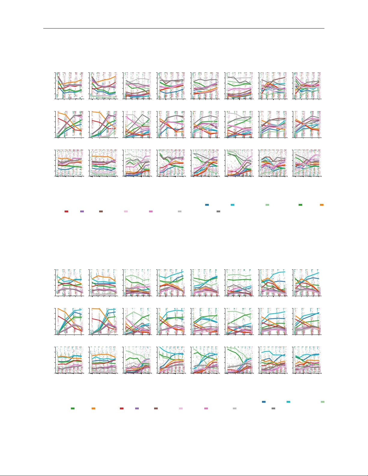
H I G H E R - O R D E R H I T - & - R U N S A M P L E R S F O R L I N E A R L Y C O N S T R A I N E D D E N S I T I E S Richard D. P aul 1 , 2 Anton Stratmann 1 Johann F . Jadebeck 1 Martin Beyß 1 Hanno Scharr 1 David Rügamer 2 , 3 Katharina Nöh 1 1 Forschungszentrum Jülich 2 Department of Statistics, LMU Munich 3 Munich Center for Machine Learning (MCML) A B S T R AC T Marko v chain Monte Carlo (MCMC) sampling of densities restricted to linearly constrained domains is an important task arising in Bayesian treatment of inv erse problems in the natural sciences. While ef ﬁcient algorithms for uniform polytope sampling e xist, much less w ork has dealt with more comple x constrained densities. In particular , gradient information as used in unconstrained MCMC is not necessarily helpful in the constrained case, where the gradient may push the proposal’ s density out of the polytope. In this work, we propose novel constrained sampling algorithms, which combine strengths of higher-order information, like the tar get log-density’ s gradients and curvature, with the Hit-&-Run proposal, a simple mechanism which guarantees the generation of feasible proposals, fulﬁlling the linear constraints. Our extensiv e experiments demonstrate improv ed sampling efﬁcienc y on complex constrained densities o ver v arious constrained and unconstrained samplers. 1 Introduction x x x + ˆ ε ∇ log ϕ ( x ) x + ˆ ε ∇ log ϕ ( x ) x + γ a v x + γ a v x + γ b v x + γ b v y y Figure 1: Our proposed smLHR sampler preconditions the direction using local curv ature and clips the natural gradient step to prev ent it from leaving the feasible region. Hit-&-Run ( HR , Smith, 1984; Bélisle et al., 1993) is a well-established Markov c hain Monte Carlo (MCMC) method for sampling from probability densities deﬁned on constrained domains. HR is applied in di verse do- mains like operations research (T ervonen et al., 2013), cosmology (Lubini et al., 2013), systems biology (Her- rmann et al., 2019; Theorell et al., 2017) and ecol- ogy (Gellner et al., 2023), where modelling principles giv e rise to linearly constrained domains. Moreover , HR has been used as a b uilding block in advanced sampling algorithms (Theorell and Nöh, 2019; Ashton et al., 2022; Łatuszy ´ nski and Rudolf, 2024). Its main strength for constrained sampling is the algorithm’ s guarantee to only generate feasible samples. Lovász and V empala (2006) prov e HR mixes rapidly for uniform sampling of bounded and con vex linearly constrained domains, referred to as con vex polytopes. Howe ver , real-world inv erse problems, e.g. those aris- ing from Bayesian inference (Theorell et al., 2017; Bo- rah Slater et al., 2023), lead to more complex non-uniform densities. These densities present additional sampling challenges such as strong nonlinear correlations between Higher-Order Hit-&-Run Samplers for Linearly Constrained Densities variables, or concentration of measure in small re gions of the constrained domain. For sampling densities deﬁned on unconstrained domains, the incorporation of higher-order information of the density has shown great success in dealing with these challenges. Prominent examples are gradient-guided samplers such as the Metr opolis-adjusted Langevin algorithm (MALA, Rossky et al., 1978) and Hamiltonian Monte Carlo (HMC, Duane et al., 1987), or curv ature-based preconditioning as in Riemannian Manifold MALA (mMALA) and Riemannian HMC (RHMC, Girolami and Calder- head, 2011). In addition, recent advances in automatic dif ferentiation have greatly beneﬁted the calculation of the higher-order information (Baydin et al., 2018). T o lev erage higher-order information for sampling densities deﬁned on conv exly constrained domains, alternativ es to HR hav e been proposed. (K ook et al., 2022) introduce a constrained version of Riemannian HMC for sampling log-concav e densities, but test it only for uniform problems. Recently , (Sriniv asan et al., 2024) proposed the ﬁrst-order Metr opolis-adjusted Pr econditioned Langevin algorithm (MAPLA). Built upon Girolami and Calderhead (2011), MAPLA preconditions a Gaussian proposal density with a metric induced by the log-barrier function (Fiacco and McCormick, 1990) to incorporate information about the constraints instead of the curvature information of the domain- constrained density . Although MAPLA aims to guide the sampling such that proposed samples respect the constraints, its proposal density remains Gaussian, thus admitting some positiv e probability of proposing infeasible samples. This raises the question whether higher-order algorithms that only propose feasible samples improve the sampling ef ﬁciency for non-uniform constrained sampling problems. Contribution In this work, we propose feasible higher-order samplers, which have positi ve proposal density just exactly on the con vex-constrained domain. T o this end, we combine the HR proposal mechanism with existing ﬁrst- and second-order samplers like MALA and the simpliﬁed mMALA(Girolami and Calderhead, 2011). As a result, we de velop three ne w samplers Langevin Hit-&-Run (LHR), simpliﬁed manifold Hit-&-Run (smHR), and simpliﬁed manifold Lange vin Hit-&-Run (smLHR). Our approach is mainly driven by the observation that a Gaussian random variable can be sampled in a HR -like fashion by decomposing it into direction and magnitude. W e provide theoretical analysis to prov e con vergence of our samplers to the desired tar get densities. W e numerically ev aluate our algorithms on a systematically constructed benchmark consisting of 2240 problems, which combine parametrizable polytopes and probability densities of v arying geometry or ill condition, as well as on real-world examples from the ﬁeld of Bayesian 13 C metabolic ﬂux analysis ( 13 C-MF A, Theorell et al., 2017). Our results sho w that our combination of both the incorporation of higher-order information and the constraining of the proposal density by the HR proposal mechanism improv e sampling efﬁcienc y . 2 Preliminaries W e consider the problem of MCMC sampling from smooth probability densities π ( x ) with support restricted to non-empty , conv ex-constrained domains P = { x ∈ R d : Ax ≤ b } , (1) deﬁned by m linear constraints Ax ≤ b , i.e. A ∈ R m × d , b ∈ R m . If P is bounded, we refer to it as a polytope . 2.1 Metropolis-Hastings Algorithm The Metr opolis-Hastings (MH, Metropolis et al., 1953; Hastings, 1970) algorithm is a widely applied method to draw samples from a target density π : R d → R , e ven if access is only provided to some unnormalized density φ ( x ) = Z π ( x ) , where Z is the normalization constant. It works by iterativ ely drawing samples, called pr oposals , from some proposal distrib ution y ∼ q ( · | x ) conditional on x , before “corr ecting” them to match the desired target distribution. T o this end, the MH algorithm adds a ﬁlter that accepts or rejects transitions from x to y with acceptance probability α ( y | x ) = min  1 , φ ( y ) φ ( x ) ·  Z  Z · q ( x | y ) q ( y | x )  . (2) A sufﬁcient condition for the con vergence of this Marko v chain is that q ( y | x ) > 0 for any two states x , y ∈ supp( π ) (Roberts and Rosenthal, 2004). The MH algorithm is also applicable to constrained target densities π : P → R , if we deﬁne an extension thereof with zero density for any state outside P , i.e. ˆ π ( x ) := 1 P ( x ) π ( x ) , where 1 P is the indicator function on P . Assuming that we start within supp( π ) ⊆ P , the MH ﬁlter pre vents the sampler to move outside of P ev en for an infeasible proposal y / ∈ P , as α ( y | x ) = 0 in that case. Thus, in principle any unconstrained proposal distribution can be used to 2 Higher-Order Hit-&-Run Samplers for Linearly Constrained Densities produce samples from constrained densities π . Ho wever , using such a proposal distribution quickly grows inef fectiv e when many infeasible y / ∈ P are proposed and, thus, immediately rejected. Hence, the dev elopment and analysis of constrained sampling algorithms has been of great interest (Smith, 1984; Bélisle et al., 1993; Lovász, 1999; Kannan and Narayanan, 2012; Narayanan, 2016; Chen et al., 2017, 2018; Mangoubi and V ishnoi, 2022; K ook et al., 2022; Gatmiry et al., 2024; Sriniv asan et al., 2024). 2.2 Hit-&-Run Sampler A simple method, which guarantees the proposal to remain within the constrained domain, is the HR algorithm (Smith, 1984; Bélisle et al., 1993): Algorithm 1 Hit-&-Run Algorithm 1: Draw a point u uniformly at random from the d − 1 dimensional hypersphere, i.e. ∥ u ∥ 2 = 1 , 2: scale the update with the step size ε , i.e. v = ε u , 3: compute the step size γ max for which x + γ max v intersects with the constraints, 4: draw a step γ ∼ p [0 ,γ max ] from the step distribution p truncated to [0 , γ γ max ] , and 5: compute the update y = x + γ v . For bre vity , we denote drawing a sample using Alg. 1 as y ∼ HR( x , ε 2 ) . The truncated step distribution has density p [0 ,γ max ] ( γ ) =  p ( γ )/ F p ( γ ) , if γ ∈ [0 , γ max ] , 0 , else (3) where F p is the cumulati ve density of the uni variate, continuous step distrib ution p and γ max is the intersection with the constraints, i.e. s :=  b 1 − a ⊤ 1 x a ⊤ 1 v , . . . , b m − a ⊤ m x a ⊤ m v  , (4) yielding the largest step size γ max from x along v such that x + γ max v ∈ P . If s has no positiv e entries, then no constraints lay ahead the direction v . In this case, we set γ max := ∞ in which case F p ( ∞ ) := 1 . Giv en γ max , p [0 ,γ max ] can be sampled using the in verse transform algorithm, if access to the cumulati ve and in verse cumulativ e density functions of p exists. The HR algorithm has, thus, the proposal density q HR ( y | x , ε ) = p [0 ,γ max ] ( ∥ y − x ∥ 2 /ε ) ( ∥ y − x ∥ 2 /ε ) d − 1 · Γ( d/ 2) 2 π d/ 2 . (5) Under the mild assumption of supp( p ) = R + , it follows that q ( y | x ) > 0 for any two x , y ∈ R d and, thus, the MH chain with HR proposal distribution con verges. In the limit of γ max → ∞ and for the particular choice of p being the χ d distribution, the HR algorithm draws samples from N ( x , ε 2 I ) . This can be seen from decomposing a Gaussian sample η ∼ N (0 , I ) into its directional and magnitudal components, u = η / ∥ η ∥ and γ = ∥ η ∥ , respecti vely . No w we observe that the direction u ∼ U S d − 1 follows a uniform distrib ution on the d − 1 hypersphere S d − 1 and the magnitude γ ∼ χ d follows a χ d distribution. 2.3 Higher -Order Sampling Algorithms In many sampling problems, access to higher -order information of the target density π is av ailable. A well-established method to incorporate ﬁrst-order information in the sampling process is MALA (Rossky et al., 1978), which proposes new samples y ∼ N  x + ε 2 2 ∇ log φ ( x ) , ε 2 I  , (6) before applying the MH ﬁlter from Eq. (2). By applying some drift ε 2 ∇ log φ ( x ) / 2 tow ards higher-density regions, MALA often achiev es higher sampling efﬁciency than zeroth-order samplers. mMALA (Girolami and Calderhead, 2011) extends the original MALA by incorporating second-order information. T o this end, mMALAlocally preconditions the MALA update using a user-speciﬁed metric tensor G ( x ) , which improv es 3 Higher-Order Hit-&-Run Samplers for Linearly Constrained Densities (a) (a) x x x + γ a v x + γ a v x + γ b v x + γ b v y y (b) (b) x x x + ˆ ε ∇ log ϕ ( x ) x + ˆ ε ∇ log ϕ ( x ) x + γ a v x + γ a v x + γ b v x + γ b v y y (c) (c) x x x + γ a v x + γ a v x + γ b v x + γ b v y y Figure 2: V isualizations of (a) HR, (b) LHR and (c) smHR on a constrained 2-dimensional toy density . A visulization of smLHR is giv en in Fig. 1. sampling efﬁcienc y for densities admitting locally varying or ill-conditioned curv ature. Ho wever , mMALA requires the gradient of the metric tensor in order to be the correct Euler-Maruyama discretization of the Riemannian Langevin diffusion on the manifold giv en by the metric tensor G ( x ) . As this can be computationally expensi ve, Girolami and Calderhead (2011) also propose a simpliﬁed mMALA (smMALA), which assumes ∂ G ( x )/ ∂ x = 0 . The resulting proposal of the simpliﬁed algorithm is then y ∼ N  x + ε 2 2 G ( x ) − 1 ∇ log φ ( x ) , ε 2 G ( x ) − 1  . (7) Although this results in a “wrong” discretization of the Riemannian Langevin dif fusion, this is a minor issue in the context of MH sampling, as the MH ﬁlter (cf. Eq. (2)) will account for the error and guarantee con ver gence to the correct target distrib ution. Indeed, as Girolami and Calderhead (2011) demonstrate empirically , assuming ∂ G ( x )/ ∂ x = 0 does improv e the sampling efﬁcienc y per unit of wall clock time, being less efﬁcient yet much f aster per sample. 3 Higher -Order Hit-&-Run In this section, we present our approach to combine the zeroth-order HR algorithm with higher-order information. Before delving into technical details, we give a more intuiti ve overvie w . Our ideas are motiv ated by the earlier mentioned observation, that the zeroth-order HR proposal distrib ution virtually becomes a diagonal Gaussian proposal distribution as the constraints “move further away” , though sampled in a manner that decomposes the sample into direction and magnitude components. No w as MALA and smMALA are also just Gaussian proposal distributions, we devise HR-lik e proposal distributions, which replicate the relationship between HR and diagonal Gaussian proposal distrib utions, but for the MALA and smMALA. 3.1 Langevin Hit-&-Run First, we consider the incorporation of gradient information into the HR proposal distribution. A ke y issue with incorporating gradients into constrained sampling stems from the fact that the gradient, if too large, may quickly push proposals out of P , turning them infeasible. Thus, we add a simple clipping mechanism by solving for the intersection of the gradient with the constraints, i.e. we choose κ as the largest positi ve entry from κ :=  b − a ⊤ 1 x a ⊤ 1 ∇ log φ ( x ) , . . . , b − a ⊤ m x a ⊤ m ∇ log φ ( x )  . (8) Similarly to Eq. (4), in the case where no positiv e entries exist in κ , we set κ := ∞ , meaning that no constraints are hit when going along the gradient ∇ log φ ( x ) . W e then clip the drift term at κ/ 2 , i.e. we choose ˆ ε = min { ε 2 / 2 , κ/ 2 } as the gradient step size. Doing so, the drifted mean of our proposal distribution can go at most halfway up until it hits the closest constraint. Using this ne w clipped step size ˆ ε , we sample our proposal as y ∼ LHR( x , ε 2 ) := HR  x + ˆ ε ∇ log φ ( x ) , ε 2  , (9) which we refer to as the Langevin Hit-&-Run ( LHR ) proposal distribution. W e decide to clip at κ/ 2 as getting exactly onto the constraints, i.e. choosing to clip at κ , can hav e unfa vorable effects when computing the intersection γ max . Howe ver , choosing exactly the halfway point κ/ 2 is purely heuristically motiv ated. As intended, in the limit of κ, γ max → ∞ , i.e. when the constraints are “far away” from x , and for p = χ d , the LHR proposal distribution simpliﬁes to MALA. 4 Higher-Order Hit-&-Run Samplers for Linearly Constrained Densities 3.2 Simpliﬁed Manifold Lange vin Hit-&-Run Next up, we incorporate curv ature information. Ignoring the drift term in smMALA for a moment, smMALA mainly preconditions the Gaussian proposal locally , i.e. let LL ⊤ = G ( x ) − 1 be the Cholesky f actorization of the in verse metric tensor , then – ignoring the drift term – smMALA samples y = ε L ⊤ η = ε ∥ η ∥ 2 L ⊤ η ∥ η ∥ 2 (10) for η ∼ N (0 , I ) . Decomposing η into its direction η / ∥ η ∥ and magnitude ∥ η ∥ , the direction follows a uniform distribution on the d − 1 hypersphere, i.e. η / ∥ η ∥ 2 ∼ U S d − 1 , and the magnitude follows a χ d -distribution, i.e. ∥ η ∥ 2 ∼ χ d . Thus, we can sample y using a slight modiﬁcation of the HR algorithm by preconditioning the directional component η / ∥ η ∥ by ε L , which – intuitiv ely speaking – results in an HR algorithm that draws the directional component from an ellipsoid rather than a hypersphere. W e call this the elliptical Hit-&-Run (EHR) algorithm, which we state for some general positiv e deﬁnite covariance matrix Σ : Algorithm 2 Elliptical Hit-&-Run Algorithm 1: Draw a point u uniformly at random from the d − 1 dimensional hypersphere, i.e. ∥ u ∥ 2 = 1 , 2: compute the update direction v = L ⊤ u , 3: compute the step size γ max for which x + γ max v intersects with the constraints, 4: draw a step γ ∼ p [0 ,γ max ] from the step distribution truncated to [0 , γ max ] , and 5: compute the update y = x + γ v . W e denote Alg. 2 in short as y ∼ EHR( x , Σ ) , for some positiv e deﬁnite matrix Σ with Cholesky factorization Σ = LL ⊤ and assume A , b , p to be given. Elliptical HR proposals are well-kno wn in the polytope sampling literature (Lovász and V empala, 2004; Haraldsdóttir et al., 2017; Theorell et al., 2022; Jadebeck et al., 2023), where they are prominently used to apply rounding transfor- mations, which make the polytope more isotropic, but can also be simply considered as a preconditioner to the HR proposal. Unlik e in our intended use case, the rounding preconditioner is constant and its contrib ution to the proposal density cancels out due to symmetry in the MH ﬁlter (cf. Eq. (2)). Howe ver , MH chains using the EHR proposal distribution with non-constant Σ ( x ) require the proposal density q EHR ( y | x , Σ ( x )) in order to compute the MH ﬁlter from Eq. (2). T o this end, we deri ve its proposal density , giv en in the following Lem. 3.1, where we denote the in verse of the transposed Cholesky factor of some symmetric positiv e deﬁnite (s.p.d.) Σ as L −⊤ := ( L ⊤ ) − 1 . The proof is provided in Sec. A of the appendix. Lemma 3.1. Assume x ∈ P and Σ s.p.d., then for y ∼ EHR( x , Σ ) , y ∈ P and has density q EHR ( y | x , Σ ) ∝ p [0 ,γ max ]  ∥ L −⊤ ( y − x ) ∥ 2  ∥ L −⊤ ( y − x ) ∥ d − 1 2 | det L | . (11) W ith the EHR and LHR algorithms now at hand, we state the simpliﬁed manifold Lange vin Hit-&-Run ( smLHR ) proposal as y ∼ smLHR( x , ε 2 ) := EHR  x + ˆ ε G ( x ) − 1 ∇ log φ ( x ) , ε 2 G ( x ) − 1  , where ˆ ε is the clipped step size as in LHR , but for the natural gradient G ( x ) − 1 ∇ log φ ( x ) . W e further consider the simpliﬁed manifold Hit-&-Run ( smHR ), which omits the gradient step of LHR and only retains the elliptical preconditioning component of smLHR y ∼ smHR( x , ε 2 ) := EHR  x , ε 2 G ( x ) − 1  . (12) This serves to empirically in vestigate the inﬂuence of the introduced changes to the HR algorithm. 3.2.1 Choice of Metric T ensors The choice of an appropriate metric is not unique (Girolami and Calderhead, 2011). While the Hessian H ( x ) := ∇ 2 log φ ( x ) of the log-density is a natural choice if the latter happens to be concave, it may not be positi ve deﬁnite in the general case, disqualifying it as a metric tensor . In Bayesian inference problems, the sum of the Fisher information 5 Higher-Order Hit-&-Run Samplers for Linearly Constrained Densities matrix and the Hessian of a strictly log-concav e prior yield a meaningful metric (Girolami and Calderhead, 2011). For Riemannian sampling of general densities, the SoftAbs (Betancourt, 2013) and the Monge metric (Hartmann et al., 2022) hav e been proposed. In this work, we additionally test two novel metrics based on the the Hessian of the log-density . The ﬁrst new metric that we introduce is the squared Hessian metric G sq ( x ) := H ( x ) ⊤ H ( x ) + δ I , (13) which has the fav orable property of being positiv e deﬁnite for δ > 0 , as the squared Hessian term being a Gram matrix is positi ve semi-deﬁnite. Ho wever , if the Hessian happens to be locally positi ve deﬁnite, the squared Hessian will apply an undesired second scaling. For this reason, we propose a heuristically motiv ated approach to adjust the scaling of the squared Hessian metric by taking the element-wise square root of its non-zero entries, i.e. let M := H ( x ) ⊤ H ( x ) ∈ R d × d with entries m ij and sgn the sign function, then the ne w scaled squared Hessian metric becomes G sc ( x ) :=  sgn( m ij ) · q | m ij |  ij + δ I . (14) As the new metric may not be positiv e deﬁnite, we use the diagonal of Eq. (14) as a surrogate metric tensor , if the Cholesky decomposition of the former fails. Controlling the Step Size In practice, the δ parameter is not known a priori and typically needs to be tuned using e.g. grid search approaches, as a too large δ makes G ( x ) more and more isotropic, effecti vely rev erting the contribution of smLHR . If δ is too small, this leads to numerical issues when G ( x ) is not positiv e deﬁnite. Hence, δ needs to be tuned for each indi vidual problem, similarly to the step size. Ho wever , noting that δ also affects the step size and in order to maintain a single tunable hyperparameter , we propose a novel kind of step size parametrization, where we keep ε = 1 ﬁxed and instead only tune δ . In order to keep this approach of controlling the step size comparable to the “classical” one, we reparametrize δ = λ − 2 and consider λ the tunable hyperparameter . T o distinguish the two approaches, we refer to the algorithms with ﬁx ed δ as smMALA ε , smHR ε , and smLHR ε , and those that ﬁx ε = 1 as smMALA δ , smHR δ and smLHR δ . Note that we can apply the δ -parametrization to general metrics G ( x ) using ˆ G ( x ) := G ( x ) + δ I as metric instead. W e e valuate both approaches experimentally in Sec. 5. 3.3 Con vergence Analysis W e state the con vergence of our algorithms under the follo wing mild assumption in Thm. 3.2: ( A1 ) The state space P ⊆ R d is con vex, ( A2 ) p is positive and continuous on R + , and ( A3 ) π is ﬁnite and twice continuously differ entiable on P . Theorem 3.2. Let P LHR , P smHR , P smLHR be the MH kernels (cf . Eq. (19) ) with pr oposal distributions LHR , smHR , smLHR , r espectively . Under assumptions A1 – 3 , for π -almost all x ∥ P n ( x , · ) − π ( · ) ∥ TV → 0 , as n → ∞ , (15) and for P being any of P LHR , P smHR , P smLHR . A proof is provided in Sec. A in the appendix, here we give a sketch of our argument. Follo wing Nummelin (1984, Theorem 3.7(i) & Prop. 6.3) and Tierne y (1994, Theorem 1), any π -irreducible, aperiodic Markov chain with in variant measure π con verges in total variation for π -almost all x ∈ P . Howev er, since the MH chain has π as its in variant measure by construction (Roberts and Rosenthal, 2004, Prop. 1 & 2), it remains to sho w π -irreducibility and aperiodicity . Aperiodicity follo ws from the ﬁniteness of π and π -irreducibility of the MH chain (Roberts and Rosenthal, 2004, Running Example). A sufﬁcient condition for π -irreducibility is positi vity and continuity of the proposal density on supp( π ) = P (Robert and Casella, 2004, Eq. (7.5)). For Eq. (11), both requirements follow from assumptions ( A1 – 2 ) and an additional assumption of Σ being s.p.d. Note that Σ being s.p.d. lies in the responsibility of the practitioner . Since our clipped gradient step does not violate the assumption of x ∈ P by construction, Thm. A.1 remains v alid. 6 Higher-Order Hit-&-Run Samplers for Linearly Constrained Densities (a) 0 0.5 1 x 0 0 0.5 1 x 1 Cone 0 0.5 1 x 0 Diamond 18 36 54 72 90 Angle θ (a) (b) 0 0.5 1 x 0 0 0.5 1 x 1 F unnel 0 0.5 1 x 0 Bowtie 0 0.5 1 x 0 Gauss 0 0.5 1 x 0 Disc 0 0.5 1 x 0 Cigar 0.01 0.1 1.0 Scale σ (b) . . . µ µ µ Figure 3: T wo-dimensional, e xemplary visualizations of the (a) polytopes and (b) densities under consideration, as well as the ef fect of the respectiv e scale σ and angle θ parameters. The mode of the Gaussian densities is controlled by µ along the (1 , . . . , 1) axis. 4 Related W ork Most work on linearly constrained sampling focuses on uniform densities. Smith (1984) introduced polytope-adapted HR. Berbee et al. (1987) combined HR with Gibbs sampling, also kno wn as Coordinate HR , which was sho wn to be fast and reliable for uniform sampling, both empirically (Emiris and Fisikopoulos, 2013) and theoretically (Laddha and V empala, 2022). Moreo ver , preconditioning (Haraldsdóttir et al., 2017) and thinning (Jadebeck et al., 2023) to minimize cost per sample were sho wn to further improve performance. Alternativ es to HR incorporate linear constraints using local preconditioning based on the Hessian of a barrier function. For example, Dikin walk uses the log-barrier (Kannan and Narayanan, 2012) and V aidya walk uses v olumetric log-barrier (Chen et al., 2017). Reﬂection-based approaches also exist (Gryazina and Polyak, 2012). Apart from uniform sampling, research has mainly explored log-concave distributions. Existing uniform samplers hav e been transformed into non-uniform ones using the MH ﬁlter and were used to sample Gaussian distributions for polytope v olume estimation (Cousins and V empala, 2015; Emiris and Fisikopoulos, 2018). Implementations for MH-based constrained sampling were provided by Jadebeck et al. (2021) & Paul et al. (2024). The ﬁrst methods to incorporate ﬁrst-order information into non-uniform constrained sampling were HMC methods, which use the gradient of their target distrib ution. T o address constraints, these methods modify the underlying Hamiltonian dynamics: K ook et al. (2022) and Noble et al. (2023) integrated penalty terms to slo w do wn particles in proximity to the boundary , while Chalkis et al. (2023) introduced a reﬂection mechanism on the boundaries. These approaches were benchmarked numerically only for truncated Gaussian or uniform target densities. Based on Girolami and Calderhead (2011) and K ook and V empala (2024), Sriniv asan et al. (2024) propose the MAPLA, a ﬁrst-order sampler for general distributions on con vex domains. MAPLA can be understood as a a smMALA variant, which uses the log-barrier’ s Hessian as metric tensor , preventing second-order information of the log-density from being easily integrated. 5 Experiments W e benchmark our algorithms experimentally on synthetic constrained densities with varying curvature or ill-conditioned cov ariance, as well as on real-world examples from the ﬁeld of Bayesian 13 C metabolic ﬂux analysis (Theorell et al., 2017). All algorithms were implemented in blackjax (Cabezas et al., 2024). W e used jax (Bradbury et al., 2018) to compute gradients and Hessians of the synthetic densities. For the 13 C-MF A problems, we used the simulation software 13CFLUX (Stratmann et al., 2025), which also provides gradient and Fisher information computations. Our blackjax fork is publicly av ailable at https://github.com/ripaul/blackjax and the code for our experiments and ﬁgures at https://github.com/ripaul/manifold- hit- and- run . All e xperiments are replicated using four different random seeds. 5.1 Synthetic Densities Problem Setup For our constrained densities, we “placed” unconstrained densities in tw o dif ferent kinds of polytopes, which we refer to as cone and diamond . Both polytopes are parametrized by an angle parameter θ ∈ (0 ◦ , 90 ◦ ] controlling its narro wness. In all cases, the constructed polytope is contained within the [0 , 1] d box. W e visualize this in Fig. 3a, more details including the generalization of our polytopes to higher dimensions are provided in Sec. B in the appendix. As densities we consider a slight modiﬁcation of Neal’ s funnel (Neal, 2003), a bowtie distribution and a total of six Gaussians with isotropic and anisotropic co variance structures and two different locations of the mean, such that the mode is once contained within the polytope ( µ = 0 . 5) and once located on the polytope’ s border ( µ = 0) . Bo wtie and 7 Higher-Order Hit-&-Run Samplers for Linearly Constrained Densities (a ) (b) µ = 0 µ = 0 . 5 Cigar / Disc / Gauss Bowtie / Funnel 9 ° 19 ° 45 ° 90 ° 0.0 0.2 0.4 0.6 0.8 1.0 Rel. Perf. → Angle 9 ° 19 ° 45 ° 90 ° 0.0 0.2 0.4 0.6 0.8 1.0 Rel. P erf. → Angle 9 ° 19 ° 45 ° 90 ° 0.0 0.2 0.4 0.6 0.8 1.0 Rel. P erf. → Angle µ = 0 µ = 0 . 5 Cigar / Disc / Gauss Bowtie / Funnel 10 − 2 10 − 1 10 0 10 1 0.0 0.2 0.4 0.6 0.8 1.0 Rel. Perf. → Scale 10 − 2 10 − 1 10 0 10 1 0.0 0.2 0.4 0.6 0.8 1.0 Rel. P erf. → Scale 10 − 2 10 − 1 10 0 10 1 0.0 0.2 0.4 0.6 0.8 1.0 Rel. P erf. → Scale (a) (b) Figure 4: Relative performance of the tested samplers on our benchmark problems as described in Sec. 5. Individual dots sho w relati ve performance of indi vidual sampling runs, the solid lines sho w average relati ve performance across all problems. Algorithms sho wn are R WMH , MALA , smMALA δ , Dikin , MAPLA , HR , LHR , smHR δ , and smLHR δ . funnel are shifted such that their mode is contained within the polytope. A visualization is gi ven in Fig. 3b, more details are provided in Sec. B in the appendix. Moreov er, we introduce a scaling parameter σ , which allo ws to control ho w close the densities’ high-probability region is to the constraints. That is, if the mode is not located at the polytope’ s border , then for small σ the target distribution may be far enough from the constraints to consider the problem ef fectively unconstrained, whereas for larger σ the target distribution approaches a uniform distrib ution on P . Finally , for our benchmark, we build our set of problems as the Cartesian product of our eight differe nt densities at log-uniformly chosen scales σ = 10 − 2 , 10 − 1 . 5 , . . . , 10 1 restricted to our two kinds of polytopes, parametrized with angles θ = 9 ◦ , 19 ◦ , 45 ◦ , 90 ◦ and for dimensions d = 2 , 4 , 8 , 16 , 32 , resulting in 2240 different test problems. Evaluation Our main criteria for the ev aluation of our algorithms are the L1 error of the joint marginal distrib ution across the ﬁrst two dimensions and the minimal marginal ef fectiv e sample size ( min ESS ), similar to Biron-Lattes et al. (2024). For the former, we ran large-scale MCMC simulations using samplers from the toolbox hopsy (Paul et al., 2024) to generate “gr ound-truth” marginal distributions. L1 error is then simply computed across the 2D histograms. W e giv e more details in Sec. B.1 in the appendix. Since the achievable min ESS depends strongly on the problem at hand, we consider the relativ e performance of an algorithm for ev ery problem as the ratio between its achiev ed av erage min ESS and the highest achiev ed av erage min ESS across replicates on the same problem. W e perform a log-uniform grid search of the step size parameter for each algorithm under consideration. and always report results for the step size achieving the smallest L1 error . W e test a Gaussian random walk MH sampler (R WMH), MALA, smMALA, Dikin, MAPLA, HR and our introduced algorithms LHR ε , smHR ε and smLHR ε , as well as LHR δ , smHR δ and smLHR δ . F or all HR v ariants, we choose p to be a half-normal distribution which moment-matches a χ d distribution, as using a χ d distribution is numerically expensiv e. For the manifold samplers, we use the Hessian as metric tensor for all Gaussian targets and test the SoftAbs (Betancourt, 2013), Monge (Hartmann et al., 2022), squared and scaled squared Hessian metrics from Eq. (13) & Eq. (14), respectiv ely , for the bowtie and funnel densities. For each experiment we run four chains, dra wing 20 000 · d samples each and thinning them down to 20 000 to reduce the memory footprint. T able 1: Mean L1 error of joint mar ginals of ﬁrst and second dimension. Best entries per column are marked in bold. Sampler Gauss / Cigar / Disc ( µ = 0 ) Gauss / Cig ar / Disc ( µ = 0 . 5 ) Bowtie / Funnel 9° 19° 45° 90° 9° 19° 45° 90° 9° 19° 45° 90° R WMH 0.373 0.094 0.046 0.047 0.045 0.043 0.049 0.051 0.05 0.045 0.05 0.052 MALA 0.374 0.093 0.045 0.045 0.043 0.042 0.047 0.049 0.046 0.043 0.048 0.051 smMALA δ 0.366 0.088 0.043 0.044 0.041 0.04 0.045 0.046 0.043 0.04 0.045 0.047 Dikin 0.028 0.034 0.045 0.049 0.042 0.045 0.051 0.053 0.037 0.043 0.05 0.054 MAPLA 0.03 0.036 0.047 0.051 0.05 0.05 0.052 0.051 0.04 0.045 0.051 0.055 HR 0.109 0.039 0.041 0.044 0.039 0.042 0.048 0.049 0.041 0.043 0.049 0.051 LHR 0.109 0.038 0.041 0.043 0.038 0.04 0.047 0.048 0.04 0.041 0.048 0.05 smHR δ 0.078 0.036 0.041 0.044 0.036 0.04 0.046 0.047 0.038 0.04 0.046 0.047 smLHR δ 0.103 0.037 0.041 0.043 0.036 0.038 0.044 0.045 0.037 0.038 0.044 0.046 Results In Fig. 4a and Fig. 4b, we show relativ e performance of the samplers as functions of the polytopes’ angle parameter and the densities’ scale parameter , respecti vely . From Fig. 4a, we observe that Dikin and MAPLA perform 8 Higher-Order Hit-&-Run Samplers for Linearly Constrained Densities T able 2: Results on 13 C-MF A problems Best entries per column are marked in bold. Sampler Stationary Spiralus Instationary Spiralus min ESS min ESS/s ˆ R min ESS min ESS/s ˆ R R WMH 0.0337 19.891 1.0052 0.0 0.0 2.4501 MALA 0.0154 4.1845 1.0061 0.0 0.0 ∞ smMALA δ 0.8667 149.5027 1.0 0.0014 0.0009 1.0278 Dikin 0.0938 55.5012 1.0011 0.0 0.0 2.5191 MAPLA 0.0231 6.0852 1.0029 0.0 0.0 ∞ HR 0.0321 13.6633 1.0031 0.0 0.0 2.4559 LHR 0.0177 3.982 1.0075 0.0 0.0 ∞ smHR δ 0.2663 62.3391 1.0001 0.0005 0.0006 1.0335 smLHR δ 0.7936 126.1378 1.0001 0.0091 0.0061 1.0015 particularly well for the more narro w polytopes ( θ = 9 ◦ , 19 ◦ ) and for the Gaussian tar get’ s with µ = 0 . F or the other problems, we observe notable impro vement in performance achie ved by our methods LHR , smHR δ , and smLHR δ . This also becomes apparent in T able 1, where Dikin and MAPLA achiev e lowest sampling error for the Gaussian target’ s at µ = 0 and θ = 9 ◦ , 19 ◦ , but are outperformed by our HR variants on all other problems. Our observations are in line with the known issues of HR in ill-conditioned polytopes, namely getting stuck in sharp “corners” (Lovász and V empala, 2004). Further , as expected, the unconstrained samplers R WMH , MALA , smMALA δ are consistently outperformed by their HR v ariants HR , LHR and smLHR δ . The decrease in performance of the unconstrained samplers is particularly noticeable in Fig. 4b, where the constraints become more inﬂuential as the scale parameter increases. Fig. 4b also re veals ho w gradient information becomes less effecti ve in the more uniform setting, as HR and smHR δ become competitiv e and even surpass their gradient-based counterparts LHR and smLHR δ as the scale parameter increases. (a) 0.0 0.2 0.4 0.6 0.8 1.0 Rel. Perf. → Monge SoftAbs Eq.(14) Eq.(15) Monge SoftAbs Eq.(14) Eq.(15) Monge SoftAbs Eq.(14) Eq.(15) Monge SoftAbs Eq.(14) Eq.(15) Monge SoftAbs Eq.(14) Eq.(15) Monge SoftAbs Eq.(14) Eq.(15) (a) (b) 0.0 0.2 0.4 0.6 0.8 1.0 H (b) Figure 5: Relati ve performance of smMALA ε , smMALA δ , smHR ε , smHR δ , smLHR ε & smLHR δ using (a) dif ferent choices of metric for the bowtie and funnel, and (b) on the Gaussian targets. Colored bars show the 25% Next, we analyze the ef fect of our proposed metrics and step size parametrization. For the bowtie and funnel targets, the combination of our scaled squared Hessian metric and the δ -parametrization from Sec. 3.2.1 achiev es highest av erage relativ e performance and lowest av er- age L1 error (cf. Figs. 5a and 6a, respectively) across smMALA , smHR , and smLHR . For the Gaussian targets, we also ﬁnd that our proposed δ -parametrization works better than the classical ε -parametrization (cf. Figs. 5b and 6b). W e suspect that despite the Hessian metric being arguably an optimal proposal cov ariance in the unconstrained Gaussian case, it fails to account for the polytope constraints. Howe ver , it remains unclear to us as to why making the proposal co variance more isotropic us- ing the δ -parametrization apparently improv es sampling efﬁcienc y in the constrained case. 5.2 13 C Metabolic Flux Analysis W e further test our algorithms on two test problems, a stationary and non-stationary Spir alus (W iechert et al., 2015), from Bayesian 13 C-MF A (Theorell et al., 2017), where the likelihood computation requires the solution of a set of ordinary differential equations, which reduces to solving a set of algebraic equations for the stationary case. Moreover , in the stationary case, so-called pool size parameters v anish, reducing the sampling problem’ s dimensionality . Where required, we use the Fisher information as metric tensor . As before, we run four chains, each dra wing 10 000 · d and 40 000 · d samples for stationary and non-stationary Spiralus , respectiv ely , and apply thinning by a factor d . Our results are presented in T able 2. For the simpler , 2-dimensional isotopically stationary Spiralus , we observe that smMALA δ yields the best performance, closely follo wed by smLHR δ . Interestingly , LHR decreases the performance o ver HR , whereas smHR δ improv es it, suggesting that curvature information is crucial for this problem. For the 9-dimensional isotopically non-stationary Spiralus , which entails non-identiﬁable as well as non-linearly correlated parameters (cf. Fig. 8), curvature information seems crucial in order to successfully sample this problem, as only smMALA δ , smHR δ , and smLHR δ are able to con ver ge within the gi ven budget. Among these, smLHR δ performs considerably better than its competitors. 9 Higher-Order Hit-&-Run Samplers for Linearly Constrained Densities 6 Conclusion W e propose higher-order HR samplers, which work well for linearly constrained, non-uniform densities, often out- performing the Dikin walk and recently introduced MAPLA in our numerical experiments. This suggests, that the combination of both the higher -order information as well as the strictly constrained HR proposal mechanism are key to impro ve the sampling efﬁcienc y for such problems. Notably , our methods seem more robust to “how far away” the constraints are from the target distribution’ s high-density region, which a priori may not be clear for any giv en constrained sampling problem. Similarly to the unconstrained case, we observ e that incorporating higher-order information typically improv es sampling efﬁcienc y . Despite HR being slower than its unconstrained counterparts (cf. Fig. 10) due to added complexity , our isotopically non-stationary 13 C-MF A example underlines that higher sampling efﬁcienc y translates into faster sampling when likelihood e valuations are e xpensive. Limitations & Future W ork Giv en the good performance of MAPLA and the Dikin walk in the “narr ow” polytopes and HR s weakness in such cases, engineering second-order methods that combine rounding transformations or barrier- based metrics with curvature estimates might strik e a balance for even more rob ust constrained samplers. While our introduced scaled squared Hessian metric and δ -parametrization of the step size for the second-order methods show empirically impro ved performance, future work needs to in vestigate whether this is more broadly applicable. Acknowledgements RDP’ s & AS’ research is funded by the Helmholtz School for Data Science in Life, Earth, and Energy (HDS-LEE). AS, JFJ, MB & KN are thankful to W olfgang W iechert for excellent working conditions. The authors gratefully acknowledge computing time on the supercomputer JURECA (Jülich Supercomputing Centre, 2021) at Forschungszentrum Jülich under grant no. hpcmfa . References Greg Ashton, Noam Bernstein, Johannes Buchner, Xi Chen, Gábor Csányi, Andre w Fowlie, Farhan Feroz, Matthew Grifﬁths, W ill Handley , Michael Habeck, Edward Higson, Michael Hobson, Anthony Lasenby , David Parkinson, Li via B Pártay , Matthe w Pitkin, Doris Schneider, Joshua S Speagle, Leah South, John V eitch, Philipp W acker , David J W ales, and David Y allup. Nested sampling for physical scientists. Nat. Rev . Methods Primers , 2(1), May 2022. Atilim Gunes Baydin, Barak A. Pearlmutter, Alex ey Andreyevich Radul, and Jeffre y Mark Siskind. Automatic Differentiation in Machine Learning: a Survey. Journal of Mac hine Learning Resear ch , 18(153):1–43, 2018. ISSN 1533-7928. Claude J. P . Bélisle, H. Edwin Romeijn, and Robert L. Smith. Hit-and-Run Algorithms for Generating Multi variate Distributions. Mathematics of Operations Researc h , 18(2):255–266, 1993. ISSN 0364-765X. Publisher: INFORMS. H. C. P . Berbee, C. G. E. Boender , A. H. G. Rinnooy Ran, C. L. Scheffer , R. L. Smith, and J. T elgen. Hit-and-run algorithms for the identiﬁcation of nonredundant linear inequalities. 37(2):184–207, 1987. ISSN 1436-4646. Michael Betancourt. A general metric for riemannian manifold hamiltonian monte carlo. In Frank Nielsen and Frédéric Barbaresco, editors, Geometric Science of Information , pages 327–334, Berlin, Heidelber g, 2013. Springer Berlin Heidelberg. ISBN 978-3-642-40020-9. Miguel Biron-Lattes, Nikola Surjanovic, Saifuddin Syed, T rev or Campbell, and Ale xandre Bouchard-Cote. autoMALA: Locally adaptiv e Metropolis-adjusted Langevin algorithm. In Pr oceedings of The 27th International Confer ence on Artiﬁcial Intelligence and Statistics , pages 4600–4608. PMLR, April 2024. ISSN: 2640-3498. Khushboo Borah Slater , Martin Beyß, Y e Xu, Jim Barber, Catia Costa, Jane Newcombe, Axel Theorell, Melanie J Bailey , Dany J V Beste, Johnjoe McFadden, and Katharina Nöh. One-shot 13 C 15 C metabolic ﬂux analysis for simultaneous quantiﬁcation of carbon and nitrogen ﬂux. Molecular Systems Biology , 19(3):e11099, 2023. James Bradbury , Roy Frostig, Peter Hawkins, Matthe w James Johnson, Chris Leary , Dougal Maclaurin, George Necula, Adam Paszke, Jake V anderPlas, Skye W anderman-Milne, and Qiao Zhang. J AX: composable transformations of Python+NumPy programs, 2018. Alberto Cabezas, Adrien Corenﬂos, Junpeng Lao, Rémi Louf, Antoine Carnec, Kaustubh Chaudhari, Reuben Cohn- Gordon, Jeremie Coullon, W ei Deng, Sam Duf ﬁeld, Gerardo Durán-Martín, Marcin Elantko wski, Dan Foreman- Macke y , Michele Gregori, Carlos Iguaran, Ravin Kumar , Martin L ysy , K evin Murphy , Juan Camilo Orduz, Karm Patel, Xi W ang, and Rob Zinko v . BlackJ AX: Composable Bayesian inference in J AX, February 2024. [cs]. 10 Higher-Order Hit-&-Run Samplers for Linearly Constrained Densities Apostolos Chalkis, V issarion Fisikopoulos, Marios P apachristou, and Elias Tsigaridas. T runcated log-conca ve sampling with reﬂectiv e hamiltonian monte carlo. 49(2):1–25, 2023. ISSN 0098-3500, 1557-7295. Y uansi Chen, Raaz Dwiv edi, Martin J. W ainwright, and Bin Y u. V aidya walk: A sampling algorithm based on the volumetric barrier . In 2017 55th Annual Allerton Confer ence on Communication, Contr ol, and Computing (Allerton) , pages 1220–1227, October 2017. Y uansi Chen, Raaz Dwiv edi, Martin J. W ainwright, and Bin Y u. Fast MCMC Sampling Algorithms on Polytopes. Journal of Mac hine Learning Researc h , 19(55):1–86, 2018. ISSN 1533-7928. Benjamin Cousins and Santosh V empala. Bypassing KLS: Gaussian cooling and an o^*(n3) volume algorithm. In Pr oceedings of the forty-seventh annual ACM symposium on Theory of Computing , ST OC ’15, pages 539–548. Association for Computing Machinery , 2015. ISBN 978-1-4503-3536-2. Simon Duane, A. D. K ennedy , Brian J. Pendleton, and Duncan Roweth. Hybrid Monte Carlo. Physics Letters B , 195 (2):216–222, September 1987. ISSN 0370-2693. Ioannis Z. Emiris and V issarion Fisikopoulos. Efﬁcient random-walk methods for approximating polytope volume, 2013. version: 1. Ioannis Z. Emiris and V issarion Fisikopoulos. Practical polytope volume approximation. 44(4):38:1–38:21, 2018. ISSN 0098-3500. Anthony V Fiacco and Garth P McCormick. Nonlinear pr ogramming . Society for Industrial and Applied Mathematics, January 1990. Khashayar Gatmiry , Jonathan Kelner , and Santosh S. V empala. Sampling Polytopes with Riemannian HMC: Faster Mixing via the Lewis W eights Barrier. In Proceedings of Thirty Seventh Conference on Learning Theory , pages 1796–1881. PMLR, June 2024. ISSN: 2640-3498. Gabriel Gellner , Ke vin McCann, and Alan Hastings. Stable div erse food webs become more common when interactions are more biologically constrained. Pr oceedings of the National Academy of Sciences , 120(31):2017, 2023. Mark Girolami and Ben Calderhead. Riemann manifold Langevin and Hamiltonian Monte Carlo methods. Journal of the Royal Statistical Society: Series B (Statistical Methodolo gy) , 73(2):123–214, 2011. ISSN 1467-9868. Elena Gryazina and Boris Polyak. Random sampling: Billiard w alk algorithm, 2012. version: 2. Hulda S Haraldsdóttir , Ben Cousins, Ines Thiele, Ronan M.T Fleming, and Santosh V empala. CHRR: coordinate hit-and-run with rounding for uniform sampling of constraint-based models. Bioinformatics , 33(11):1741–1743, June 2017. ISSN 1367-4803. Marcelo Hartmann, Mark Girolami, and Arto Klami. Lagrangian manifold monte carlo on monge patches. In Gustau Camps-V alls, Francisco J. R. Ruiz, and Isabel V alera, editors, Pr oceedings of The 25th International Confer ence on Artiﬁcial Intelligence and Statistics , v olume 151 of Pr oceedings of Machine Learning Resear ch , pages 4764–4781. PMLR, 28–30 Mar 2022. W . K. Hastings. Monte Carlo Sampling Methods Using Markov Chains and Their Applications. Biometrika , 57(1): 97–109, 1970. ISSN 0006-3444. Publisher: [Oxford Uni versity Press, Biometrika T rust]. Helena A. Herrmann, Beth C. Dyson, Luc y V ass, Giles N. Johnson, and Jean-Marc Schwartz. Flux sampling is a powerful tool to study metabolism under changing en vironmental conditions. npj Systems Biology and Applications , 5(1):32, 2019. Johann F Jadebeck, Axel Theorell, Samuel Le weke, and Katharina Nöh. HOPS: high-performance library for (non- )uniform sampling of con vex-constrained models. Bioinformatics , 37(12):1776–1777, July 2021. ISSN 1367-4803, 1367-4811. Johann F . Jadebeck, W olfgang W iechert, and Katharina Nöh. Practical sampling of constraint-based models: Optimized thinning boosts CHRR performance. PLOS Computational Biology , 19(8):e1011378, August 2023. ISSN 1553-7358. Publisher: Public Library of Science. Jülich Supercomputing Centre. JURECA: Data Centric and Booster Modules implementing the Modular Super- computing Architecture at Jülich Supercomputing Centre. Journal of lar ge-scale resear ch facilities , 7(A182), 2021. Ravindran Kannan and Hariharan Narayanan. Random W alks on Polytopes and an Af ﬁne Interior Point Method for Linear Programming. Mathematics of Operations Resear ch , 37(1):1–20, February 2012. ISSN 0364-765X. Publisher: INFORMS. Y unbum K ook and Santosh S. V empala. Gaussian cooling and dikin walks: The interior-point method for logconcav e sampling, 2024. 11 Higher-Order Hit-&-Run Samplers for Linearly Constrained Densities Y unbum K ook, Y inT at Lee, Ruoqi Shen, and Santosh V empala. Sampling with Riemannian Hamiltonian Monte Carlo in a Constrained Space. October 2022. Aditi Laddha and Santosh V empala. Con ver gence of gibbs sampling: Coordinate hit-and-run mix es fast, 2022. Krzysztof Łatuszy ´ nski and Daniel Rudolf. Conv ergence of hybrid slice sampling via spectral gap. Advances in Applied Pr obability , 56(4):1440–1466, 2024. Y ifang Li and Sujit K. Ghosh. Efﬁcient sampling methods for truncated multiv ariate normal and student-t distributions subject to linear inequality constraints. Journal of Statistical Theory and Pr actice , 9(4):712–732, Dec 2015. ISSN 1559-8616. László Lo vász. Hit-and-run mixes fast. Mathematical Pr ogramming , 86(3):443–461, December 1999. ISSN 1436-4646. László Lovász and Santosh V empala. Hit-and-run from a corner . In Pr oceedings of the thirty-sixth annual A CM symposium on Theory of computing , ST OC ’04, pages 310–314, Ne w Y ork, NY , USA, June 2004. Association for Computing Machinery . ISBN 978-1-58113-852-8. László Lovász and Santosh V empala. Hit-and-run from a corner . SIAM Journal on Computing , 35(4):985–1005, 2006. M. Lubini, M. Sereno, J. Coles, Ph. Jetzer , and P . Saha. Cosmological parameter determination in free-form strong gravitational lens modelling. Monthly Notices of the Royal Astr onomical Society , 437(3):2461–2470, 2013. Oren Mangoubi and Nisheeth K. V ishnoi. Sampling from Log-Concav e Distributions with Inﬁnity-Distance Guarantees. October 2022. Nicholas Metropolis, Arianna W . Rosenbluth, Marshall N. Rosenbluth, Augusta H. T eller , and Edward T eller . Equation of State Calculations by Fast Computing Machines. The Journal of Chemical Physics , 21(6):1087–1092, June 1953. ISSN 0021-9606, 1089-7690. Hariharan Narayanan. Randomized interior point methods for sampling and optimization. The Annals of Applied Pr obability , 26(1):597–641, February 2016. ISSN 1050-5164, 2168-8737. Publisher: Institute of Mathematical Statistics. Radford M. Neal. Slice sampling. The Annals of Statistics , 31(3):705–767, June 2003. ISSN 0090-5364, 2168-8966. Publisher: Institute of Mathematical Statistics. Maxence Noble, V alentin De Bortoli, and Alain Durmus. Unbiased constrained sampling with self-concordant barrier hamiltonian monte carlo, 2023. Esa Nummelin. General Irr educible Markov Chains and Non-Ne gative Operators . Cambridge Tracts in Mathematics. Cambridge Univ ersity Press, Cambridge, 1984. ISBN 978-0-521-60494-9. Richard D Paul, Johann F Jadebeck, Anton Stratmann, W olfgang W iechert, and Katharina Nöh. hopsy — a methods marketplace for con vex polytope sampling in Python. Bioinformatics , 40(7):btae430, July 2024. ISSN 1367-4811. Christian P . Robert and George Casella. Monte Carlo Statistical Methods . Springer T exts in Statistics. Springer , Ne w Y ork, NY , 2004. ISBN 978-1-4419-1939-7 978-1-4757-4145-2. Gareth O. Roberts and Jef frey S. Rosenthal. General state space Markov chains and MCMC algorithms. Pr obability Surve ys , 1(none):20–71, January 2004. ISSN 1549-5787, 1549-5787. Publisher: Institute of Mathematical Statistics and Bernoulli Society . P . J. Rossky , J. D. Doll, and H. L. Friedman. Brownian dynamics as smart Monte Carlo simulation. The Journal of Chemical Physics , 69(10):4628–4633, Nov ember 1978. ISSN 0021-9606. Robert L. Smith. Ef ﬁcient Monte Carlo Procedures for Generating Points Uniformly Distributed Over Bounded Regions. Operations Resear ch , 32(6):1296–1308, 1984. ISSN 0030-364X. Publisher: INFORMS. V ishwak Sriniv asan, Andre W ibisono, and Ashia C. Wilson. High-accuracy sampling from constrained spaces with the Metropolis-adjusted Preconditioned Langevin Algorithm. In 36th International Conference on Algorithmic Learning Theory , December 2024. Anton Stratmann, Martin Beyß, Johann F Jadebeck, W olfgang Wiechert, and Katharina Nöh. 13CFLUX - third- generation high-performance engine for isotopically (non)stationary 13 C metabolic ﬂux analysis. Bioinformatics , 41 (12):btaf630, 11 2025. ISSN 1367-4811. T ommi T ervonen, Gert v an V alkenhoef, Nalan Ba ¸ stürk, and Douwe Postmus. Hit-and-run enables efﬁcient weight generation for simulation-based multiple criteria decision analysis. European J ournal of Operational Resear ch , 224 (3):552–559, 2013. ISSN 0377-2217. Axel Theorell and Katharina Nöh. Rev ersible jump mcmc for multi-model inference in metabolic ﬂux analysis. Bioinformatics , 36(1):232–240, 06 2019. ISSN 1367-4803. 12 Higher-Order Hit-&-Run Samplers for Linearly Constrained Densities Axel Theorell, Samuel Le weke, W olfgang W iechert, and Katharina Nöh. T o be certain about the uncertainty: Bayesian statistics for 13C metabolic ﬂux analysis. Biotechnology and Bioengineering , 114(11):2668–2684, 2017. ISSN 1097-0290. Axel Theorell, Johann F Jadebeck, Katharina Nöh, and Jör g Stelling. PolyRound: polytope rounding for random sampling in metabolic networks. Bioinformatics , 38(2):566–567, January 2022. ISSN 1367-4803. Luke T ierney . Markov Chains for Exploring Posterior Distributions. The Annals of Statistics , 22(4):1701–1728, 1994. ISSN 0090-5364. Publisher: Institute of Mathematical Statistics. W olfgang W iechert, Sebastian Niedenführ , and Katharina Nöh. A Primer to 13 C Metabolic Flux Analysis , chapter 5, pages 97–142. John W iley & Sons, Ltd, 2015. ISBN 9783527697441. 13 Higher-Order Hit-&-Run Samplers for Linearly Constrained Densities A Missing Proofs In this section we present missing proofs for Thm. 3.1 and Thm. 3.2. W e be gin with a proof of the EHR density (cf. Eq. (11)): Pr oof of Thm. 3.1. Let ∆ := y − x = γ v , then step size and direction on the ellipsoid are recov ered as ∥ L −⊤ ∆ ∥ 2 = γ ∥ L −⊤ L ⊤ u ∥ 2 = γ , since ∥ u ∥ 2 = 1 and v = ∆ /γ . This transformation is a change of basis from Cartesian to spherical coordinates with differential volume d∆ = | det L | · γ d − 1 · d γ d ω , thus, the Jacobian determinant of the bijection ∆ = γ L ⊤ u is     ∂ ∆ ∂ ( γ , u )     = | det L | · γ d − 1 (16) and by the in verse function theorem, the Jacobian determinant of the inv erse map is the in verse of the Jacobian determinant of the forward map, i.e.     ∂ ( γ , u ) ∂ ∆     =     ∂ ∆ ∂ ( γ , u )     − 1 = 1 | det L | · γ d − 1 . (17) Now by transform of random v ariables, we hav e that q HR ( y | x , Σ ) = p ( γ , u | x , Σ )     ∂ ( γ , u ) ∂ ∆     = p ( γ | u , x , Σ ) p ( u ) | det L | · γ d − 1 = p ( γ | u , x , Σ ) | det L | · γ d − 1 Γ( d/ 2) 2 π d/ 2 , (18) where the last equality follows from p ( u ) = 1 / A d − 1 being the uniform distribution on the surface of the d − 1 hypersphere, which has area A d − 1 = 2 π d/ 2 / Γ( d/ 2) . Finally , p ( γ | u , x , Σ ) is just the truncated step density p [0 ,γ max ] ( γ ) as deﬁned in Alg. 2. Recalling our earlier deﬁnitions, we hav e that γ = ∥ L −⊤ ( y − x ) ∥ 2 , thus recov ering Eq. (11). Next, we ﬁll out the technical details of our sketched con vergence ar gument from Sec. 3.3. Let P ( x , y ) := α ( y | x ) q ( y | x ) + (1 − r ( x )) δ x ( y ) , with r ( x ) := Z P α ( z | x ) q ( z | x ) d z (19) be the Metr opolis kernel , where δ x ( y ) is the Dirac measure on x , α ( y | x ) is the MH ﬁlter (cf. Eq. (2)) and q ( · | x ) is some proposal distribution conditionally on x . Moreover , P n ( x , y ) = Z P P n − 1 ( x , z ) P ( z , y ) d z (20) is the recursiv ely deﬁned n -step kernel with P 0 ( x , y ) := δ x ( y ) . As discussed in Sec. 3.3, for a positive proposal distrib ution, i.e. q ( y | x ) > 0 for any two x , y ∈ P , con vergence of the n -step kernel to the desired target distrib ution is given by standard arguments under assumption ( A3 ) , as positivity then implies π -irreducibility and aperiodicity , and thus conv ergence (Roberts and Rosenthal, 2004). Therefore, it only remains to show that our algorithms’ proposal density is indeed positiv e. T o show this, we ﬁrst prove that q EHR ( · | x ) is positiv e for any x ∈ P under assumptions A1 – 2 and additionally if Σ is positive deﬁnite. Lemma A.1. Let p be positive and continuous on R , Σ = LL ⊤ s.p.d. Then, q EHR ( y | x , Σ ) = p [0 ,γ max ]  ∥ L −⊤ ( y − x ) ∥ 2  ∥ L −⊤ ( y − x ) ∥ d − 1 2 | det L | · Γ( d/ 2) 2 π d/ 2 is positive and continuous for all x , y ∈ P with x  = y . Pr oof. W e prove positivity by contradiction. Assume y ∈ P with q EHR ( y | x , Σ ) = 0 . By regularity of Σ = LL ⊤ , we always ﬁnd u = L −⊤ ( y − x ) / γ such that y = γ Lu + x for some γ . By con ve xity , we have that γ ∈ [0 , γ max ] , howe ver by positi vity of p on R , it follo ws that p [ γ a ,γ b ] ( γ ) > 0 and thus q EHR ( y | x , Σ ) > 0 , which is a contradiction. Finally , q EHR ( y | x , Σ ) is a chain of continuous functions and thereby continuous itself. Giv en Thm. A.1, we now state the proof of Thm. 3.2. 14 Higher-Order Hit-&-Run Samplers for Linearly Constrained Densities Pr oof of Thm. 3.2. By Thm. A.1 and the argument pro vided in Sec. 3.3, con ver gence of any of our three algorithms follows if we sho w that Σ is s.p.d. and the clipped gradient step remains within P . LHR: Since LHR( x , ε 2 ) = EHR( · | x + ˆ ε ∇ log φ ( x ) , ε 2 I ) , we hav e that ε 2 I is s.p.d. for ε > 0 and it only remains to sho w that x + ˆ ε ∇ log φ ( x ) ∈ P , which howe ver follows from con vexity since x , x + κ ∇ log φ ( x ) ∈ P and ˆ ε ∈ (0 , κ/ 2] . Therefore, P LHR con verges in total v ariation distance to the desired target distrib ution. smHR: For smHR( x , ε 2 ) = EHR( · | x , ε 2 G ( x ) − 1 ) it is only necessary to sho w that G ( x ) is s.p.d., as the in verse of an s.p.d. matrix is itself s.p.d., which howe ver follows from construction in Eq. (14) and for δ large enough. Therefore, P smHR con verges in total v ariation distance to the desired target distribution. smLHR: Conv ergence of P smLHR follows directly from that of P LHR and P smHR . B Experiment Details B.1 Ground T ruth Sampling W e collect “ground truth” samples from our synthetic densities by running large MCMC simulations using the HR sampler from the toolbox hopsy . F or each problem, we run four parallel chains. F or the bo wtie and funnel, we dra w 1 000 000 · d log 2 d samples using the HR sampler with a Gaussian step distrib ution with step size being the scale parameter σ of the respectiv e target. F or the Gaussian targets, we dra w 100 000 · d log 2 d samples using the truncated Gaussian sampler (Li and Ghosh, 2015). B.2 Synthetic Densities Densities As densities we consider Neal’ s funnel (Neal, 2003), with x 1 ∼ N (0 , 9) , x i ∼ N (0 , e x 1 ) , i = 2 , . . . , d, a bowtie distribution with x 1 ∼ N (0 , 1) , x i ∼ N  0 , x 2 1 / 4 + 0 . 1  , i = 2 , . . . , d, and six differently parametrized Gaussians: an isotropic, zero-centered Gaussian, a disc-like zero-centered Gaussian with marginal v ariances σ 2 1 = 1 / 100 and σ i = 1 , i = 1 , . . . , d , and a cigar-lik e zero-centered Gaussian with marginal variances σ 2 1 = 1 and σ i = 1 / 100 , i = 1 , . . . , d . W e consider two dif f erent versions of those three Gaussian targets, where the mode is either located at the origin or on the midpoint between origin and the intersection of the (1 , . . . , 1) vectir with the polytope borders, which guarantees that the mode will be contained in the polytope P . Moreover , we apply a multiv ariate location-scale transformation φ ( x ) := φ 0  Q ⊤  x − m σ   , (21) where Q ⊤ rotates the (1 , 0 , . . . , 0) vector to (1 , . . . , 1) . For the funnel and bo wtie distributions, m is determined as the halfway point between the origin and the intersection of the (1 , . . . , 1) vector with the polytope, which is supposed to keep the “characteristic” regions of the density inside the polytope. For the Gaussian distrib utions, we set m = 0 . Polytopes The cone is constructed as a simplex with tilted sides and a scaled constraint in Eq. (23), which bounds the polytope within the [0 , 1] d box: cos( θ ) · x i − sin( θ ) · x j ≤ 0 for any two dif ferent i, j = 1 , . . . , d, (22) d X i =1 x i ≤ cos( θ ) sin( θ ) + 1 . (23) The diamond is constructed as a [0 , 1] d whose sides are also tilted and scaled such that the resulting parallelogram is contained in the [0 , 1] d box: cos( θ ) · x i − sin( θ ) · x j ≤ 0 for any two dif ferent i, j = 1 , . . . , d, (24) − cos( θ ) · x i + sin( θ ) · x j ≤ sin( θ ) − cos( θ ) for any two dif ferent i, j = 1 , . . . , d. (25) C Additional Figures & T ables W e provide additional ﬁgures. In Fig. 6a & 6b, we provide L1 error results based on the used metric. In Fig. 7 & 8, we provide pair plots of the two-dimensional marginal parameter posterior distrib utions, sampled using our smLHR δ 15 Higher-Order Hit-&-Run Samplers for Linearly Constrained Densities sampler . Fig. 9, 10 & 11 further dissect the performance of the various tested samplers. For better accessibility , we provide these results also in tab ular format. (a) 0.1 1.0 L1 error ← Monge SoftAbs Eq.(14) Eq.(15) Monge SoftAbs Eq.(14) Eq.(15) Monge SoftAbs Eq.(14) Eq.(15) Monge SoftAbs Eq.(14) Eq.(15) Monge SoftAbs Eq.(14) Eq.(15) Monge SoftAbs Eq.(14) Eq.(15) (a) (b) 10 − 1 10 0 H (b) Figure 6: L1 error of smMALA ε , smMALA δ , smHR ε , smHR δ , smLHR ε & smLHR δ using (a) different choices of metric for the bowtie and funnel, and (b) on the Gaussian targets. Colored bars sho w the 25% 0 . 6 0 . 7 q 0 . 85 0 . 90 0 . 95 1 . 00 1 . 05 1 . 10 1 . 15 u Figure 7: Pair plot of parameter posterior dis- tribution of the isotopically stationary Spiralus model, sampled using our smLHR δ method. Parameter names follow W iechert et al. (2015). 0 . 9 1 . 0 1 . 1 u 10 20 30 40 50 H 20 40 60 80 G 20 40 60 80 F 20 40 60 80 E 10 20 30 C 10 20 30 40 B 0 . 55 0 . 60 0 . 65 0 . 70 q 10 20 30 40 50 D 0 . 9 1 . 0 1 . 1 u 20 40 H 25 50 75 G 25 50 75 F 25 50 75 E 10 20 30 C 20 40 B Figure 8: Pair plot of parameter posterior distrib ution of the isotopically non-stationary Spiralus model, sampled using our smLHR δ method. P arameter names follo w W iechert et al. (2015). 16 Higher-Order Hit-&-Run Samplers for Linearly Constrained Densities Gauss ( µ = 0) Disc ( µ = 0) Cigar ( µ = 0) Gauss ( µ = 0 . 5) Disc ( µ = 0 . 5) Cigar ( µ = 0 . 5) Bowtie Funnel 2 4 8 16 32 0.0 0.2 0.4 0.6 0.8 1.0 Rel. Perf. → Dimension 2 4 8 16 32 0.0 0.2 0.4 0.6 0.8 1.0 Rel. P erf. → Dimension 2 4 8 16 32 0.0 0.2 0.4 0.6 0.8 1.0 Rel. P erf. → Dimension 2 4 8 16 32 0.0 0.2 0.4 0.6 0.8 1.0 Rel. P erf. → Dimension 2 4 8 16 32 0.0 0.2 0.4 0.6 0.8 1.0 Rel. P erf. → Dimension 2 4 8 16 32 0.0 0.2 0.4 0.6 0.8 1.0 Rel. P erf. → Dimension 2 4 8 16 32 0.0 0.2 0.4 0.6 0.8 1.0 Rel. P erf. → Dimension 2 4 8 16 32 0.0 0.2 0.4 0.6 0.8 1.0 Rel. P erf. → Dimension 9 ° 19 ° 45 ° 90 ° 0.0 0.2 0.4 0.6 0.8 1.0 Rel. Perf. → Angle 9 ° 19 ° 45 ° 90 ° 0.0 0.2 0.4 0.6 0.8 1.0 Rel. P erf. → Angle 9 ° 19 ° 45 ° 90 ° 0.0 0.2 0.4 0.6 0.8 1.0 Rel. P erf. → Angle 9 ° 19 ° 45 ° 90 ° 0.0 0.2 0.4 0.6 0.8 1.0 Rel. P erf. → Angle 9 ° 19 ° 45 ° 90 ° 0.0 0.2 0.4 0.6 0.8 1.0 Rel. P erf. → Angle 9 ° 19 ° 45 ° 90 ° 0.0 0.2 0.4 0.6 0.8 1.0 Rel. P erf. → Angle 9 ° 19 ° 45 ° 90 ° 0.0 0.2 0.4 0.6 0.8 1.0 Rel. P erf. → Angle 9 ° 19 ° 45 ° 90 ° 0.0 0.2 0.4 0.6 0.8 1.0 Rel. P erf. → Angle 10 − 2 10 − 1 10 0 10 1 0.0 0.2 0.4 0.6 0.8 1.0 Rel. Perf. → Scale 10 − 2 10 − 1 10 0 10 1 0.0 0.2 0.4 0.6 0.8 1.0 Rel. P erf. → Scale 10 − 2 10 − 1 10 0 10 1 0.0 0.2 0.4 0.6 0.8 1.0 Rel. P erf. → Scale 10 − 2 10 − 1 10 0 10 1 0.0 0.2 0.4 0.6 0.8 1.0 Rel. P erf. → Scale 10 − 2 10 − 1 10 0 10 1 0.0 0.2 0.4 0.6 0.8 1.0 Rel. P erf. → Scale 10 − 2 10 − 1 10 0 10 1 0.0 0.2 0.4 0.6 0.8 1.0 Rel. P erf. → Scale 10 − 2 10 − 1 10 0 10 1 0.0 0.2 0.4 0.6 0.8 1.0 Rel. P erf. → Scale 10 − 2 10 − 1 10 0 10 1 0.0 0.2 0.4 0.6 0.8 1.0 Rel. P erf. → Scale Figure 9: Detailed presentation of relativ e performance of the tested samplers on our benchmark problems as described in Sec. 5. Indi vidual dots show relati ve performance of indi vidual sampling runs, the solid lines show av erage relative performance across all problems. Algorithms sho wn are R WMH , MALA , smMALA ε smMALA δ , Dikin , MAPLA , HR , LHR , smHR ε , smHR δ , smLHR ε , and smLHR δ . Gauss ( µ = 0) Disc ( µ = 0) Cigar ( µ = 0) Gauss ( µ = 0 . 5) Disc ( µ = 0 . 5) Cigar ( µ = 0 . 5) Bowtie Funnel 2 4 8 16 32 0.0 0.2 0.4 0.6 0.8 1.0 Rel. Perf. → Dimension 2 4 8 16 32 0.0 0.2 0.4 0.6 0.8 1.0 Rel. P erf. → Dimension 2 4 8 16 32 0.0 0.2 0.4 0.6 0.8 1.0 Rel. P erf. → Dimension 2 4 8 16 32 0.0 0.2 0.4 0.6 0.8 1.0 Rel. P erf. → Dimension 2 4 8 16 32 0.0 0.2 0.4 0.6 0.8 1.0 Rel. P erf. → Dimension 2 4 8 16 32 0.0 0.2 0.4 0.6 0.8 1.0 Rel. P erf. → Dimension 2 4 8 16 32 0.0 0.2 0.4 0.6 0.8 1.0 Rel. P erf. → Dimension 2 4 8 16 32 0.0 0.2 0.4 0.6 0.8 1.0 Rel. P erf. → Dimension 9 ° 19 ° 45 ° 90 ° 0.0 0.2 0.4 0.6 0.8 1.0 Rel. Perf. → Angle 9 ° 19 ° 45 ° 90 ° 0.0 0.2 0.4 0.6 0.8 1.0 Rel. P erf. → Angle 9 ° 19 ° 45 ° 90 ° 0.0 0.2 0.4 0.6 0.8 1.0 Rel. P erf. → Angle 9 ° 19 ° 45 ° 90 ° 0.0 0.2 0.4 0.6 0.8 1.0 Rel. P erf. → Angle 9 ° 19 ° 45 ° 90 ° 0.0 0.2 0.4 0.6 0.8 1.0 Rel. P erf. → Angle 9 ° 19 ° 45 ° 90 ° 0.0 0.2 0.4 0.6 0.8 1.0 Rel. P erf. → Angle 9 ° 19 ° 45 ° 90 ° 0.0 0.2 0.4 0.6 0.8 1.0 Rel. P erf. → Angle 9 ° 19 ° 45 ° 90 ° 0.0 0.2 0.4 0.6 0.8 1.0 Rel. P erf. → Angle 10 − 2 10 − 1 10 0 10 1 0.0 0.2 0.4 0.6 0.8 1.0 Rel. Perf. → Scale 10 − 2 10 − 1 10 0 10 1 0.0 0.2 0.4 0.6 0.8 1.0 Rel. P erf. → Scale 10 − 2 10 − 1 10 0 10 1 0.0 0.2 0.4 0.6 0.8 1.0 Rel. P erf. → Scale 10 − 2 10 − 1 10 0 10 1 0.0 0.2 0.4 0.6 0.8 1.0 Rel. P erf. → Scale 10 − 2 10 − 1 10 0 10 1 0.0 0.2 0.4 0.6 0.8 1.0 Rel. P erf. → Scale 10 − 2 10 − 1 10 0 10 1 0.0 0.2 0.4 0.6 0.8 1.0 Rel. P erf. → Scale 10 − 2 10 − 1 10 0 10 1 0.0 0.2 0.4 0.6 0.8 1.0 Rel. P erf. → Scale 10 − 2 10 − 1 10 0 10 1 0.0 0.2 0.4 0.6 0.8 1.0 Rel. P erf. → Scale Figure 10: Detailed presentation of relati ve performance based on min ESS /s of the tested samplers on our benchmark problems as described in Sec. 5. Individual dots sho w relati ve performance of indi vidual sampling runs, the solid lines show a verage relativ e performance across all problems. Algorithms shown are R WMH , MALA , smMALA ε smMALA δ , Dikin , MAPLA , HR , LHR , smHR ε , smHR δ , smLHR ε , and smLHR δ . 17 Higher-Order Hit-&-Run Samplers for Linearly Constrained Densities Gauss ( µ = 0) Disc ( µ = 0) Cigar ( µ = 0) Gauss ( µ = 0 . 5) Disc ( µ = 0 . 5) Cigar ( µ = 0 . 5) Bowtie Funnel 2 4 8 16 32 0.1 1.0 L1 error ← Dimension 2 4 8 16 32 0.1 1.0 L1 error ← Dimension 2 4 8 16 32 0.1 1.0 L1 error ← Dimension 2 4 8 16 32 0.1 1.0 L1 error ← Dimension 2 4 8 16 32 0.1 1.0 L1 error ← Dimension 2 4 8 16 32 0.1 1.0 L1 error ← Dimension 2 4 8 16 32 0.1 1.0 L1 error ← Dimension 2 4 8 16 32 0.1 1.0 L1 error ← Dimension 9 ° 19 ° 45 ° 90 ° 0.1 1.0 L1 error ← Angle 9 ° 19 ° 45 ° 90 ° 0.1 1.0 L1 error ← Angle 9 ° 19 ° 45 ° 90 ° 0.1 1.0 L1 error ← Angle 9 ° 19 ° 45 ° 90 ° 0.1 1.0 L1 error ← Angle 9 ° 19 ° 45 ° 90 ° 0.1 1.0 L1 error ← Angle 9 ° 19 ° 45 ° 90 ° 0.1 1.0 L1 error ← Angle 9 ° 19 ° 45 ° 90 ° 0.1 1.0 L1 error ← Angle 9 ° 19 ° 45 ° 90 ° 0.1 1.0 L1 error ← Angle 10 − 2 10 − 1 10 0 10 1 0.1 1.0 L1 error ← Scale 10 − 2 10 − 1 10 0 10 1 0.1 1.0 L1 error ← Scale 10 − 2 10 − 1 10 0 10 1 0.1 1.0 L1 error ← Scale 10 − 2 10 − 1 10 0 10 1 0.1 1.0 L1 error ← Scale 10 − 2 10 − 1 10 0 10 1 0.1 1.0 L1 error ← Scale 10 − 2 10 − 1 10 0 10 1 0.1 1.0 L1 error ← Scale 10 − 2 10 − 1 10 0 10 1 0.1 1.0 L1 error ← Scale 10 − 2 10 − 1 10 0 10 1 0.1 1.0 L1 error ← Scale Figure 11: Detailed presentation of av erage L1 error of the tested samplers on our benchmark problems as described in Sec. 5. Indi vidual dots show relati ve performance of indi vidual sampling runs, the solid lines show a verage relativ e performance across all problems. Algorithms sho wn are R WMH , MALA , smMALA ε smMALA δ , Dikin , MAPLA , HR , LHR , smHR ε , smHR δ , smLHR ε , and smLHR δ . 18 Higher-Order Hit-&-Run Samplers for Linearly Constrained Densities T able 3: A verage relati ve performance of the tested samplers across dimensions as presented as solid lines in Fig. 9. Sampler T arget d Gauss ( µ = 0) Disc ( µ = 0) Cigar ( µ = 0) Gauss ( µ = 0 . 5) Disc ( µ = 0 . 5) Cigar ( µ = 0 . 5) Bowtie Funnel 2 4 8 16 32 2 4 8 16 32 2 4 8 16 32 2 4 8 16 32 2 4 8 16 32 2 4 8 16 32 2 4 8 16 32 2 4 8 16 32 R WMH 0.13 0.067 0.074 0.09 0.116 0.414 0.279 0.272 0.164 0.226 0.467 0.219 0.263 0.247 0.318 0.118 0.047 0.077 0.101 0.159 0.246 0.2 0.24 0.29 0.368 0.297 0.211 0.247 0.29 0.369 0.308 0.374 0.291 0.253 0.259 0.471 0.273 0.334 0.282 0.333 MALA 0.176 0.089 0.101 0.096 0.122 0.582 0.35 0.332 0.207 0.261 0.683 0.3 0.343 0.254 0.337 0.137 0.06 0.1 0.143 0.212 0.317 0.29 0.251 0.307 0.39 0.646 0.497 0.495 0.43 0.51 0.328 0.341 0.55 0.573 0.591 0.392 0.318 0.437 0.368 0.49 smMALA ε 0.58 0.593 0.509 0.432 0.376 0.094 0.073 0.053 0.065 0.084 0.65 0.295 0.338 0.269 0.334 0.68 0.645 0.619 0.585 0.628 0.544 0.41 0.371 0.315 0.399 0.625 0.494 0.471 0.437 0.515 0.224 0.152 0.223 0.215 0.224 0.398 0.15 0.26 0.303 0.328 smMALA δ 0.58 0.401 0.43 0.352 0.183 0.588 0.346 0.333 0.22 0.26 0.653 0.301 0.358 0.281 0.348 0.59 0.495 0.52 0.575 0.557 0.645 0.58 0.455 0.508 0.55 0.622 0.53 0.46 0.477 0.512 0.495 0.445 0.463 0.33 0.366 0.688 0.38 0.393 0.483 0.499 Dikin 0.158 0.148 0.137 0.179 0.253 0.619 0.653 0.719 0.758 0.854 0.554 0.581 0.633 0.645 0.731 0.102 0.083 0.095 0.128 0.211 0.206 0.253 0.275 0.347 0.436 0.312 0.386 0.419 0.457 0.527 0.377 0.628 0.523 0.38 0.38 0.337 0.545 0.512 0.438 0.517 MAPLA 0.103 0.13 0.127 0.142 0.201 0.38 0.405 0.471 0.501 0.624 0.4 0.413 0.5 0.472 0.554 0.163 0.121 0.124 0.192 0.235 0.186 0.214 0.239 0.282 0.375 0.332 0.398 0.429 0.47 0.52 0.208 0.544 0.521 0.407 0.391 0.207 0.466 0.503 0.447 0.534 HR 0.207 0.147 0.137 0.171 0.216 0.734 0.513 0.485 0.466 0.485 0.804 0.515 0.499 0.522 0.549 0.139 0.114 0.137 0.186 0.264 0.329 0.381 0.418 0.528 0.619 0.481 0.438 0.429 0.496 0.584 0.367 0.475 0.374 0.377 0.416 0.56 0.446 0.446 0.443 0.499 LHR 0.261 0.208 0.226 0.291 0.313 0.833 0.522 0.435 0.47 0.419 0.85 0.512 0.539 0.534 0.491 0.195 0.175 0.199 0.258 0.358 0.38 0.37 0.366 0.513 0.539 0.817 0.575 0.708 0.674 0.693 0.404 0.47 0.713 0.769 0.813 0.487 0.462 0.529 0.514 0.64 smHR ε 0.557 0.542 0.496 0.515 0.53 0.311 0.145 0.126 0.14 0.185 0.77 0.534 0.498 0.534 0.545 0.402 0.375 0.317 0.379 0.439 0.361 0.222 0.253 0.306 0.38 0.463 0.443 0.422 0.506 0.588 0.449 0.362 0.286 0.298 0.267 0.536 0.468 0.414 0.439 0.492 smHR δ 0.533 0.578 0.44 0.472 0.524 0.688 0.521 0.486 0.465 0.469 0.804 0.518 0.499 0.526 0.559 0.305 0.394 0.402 0.377 0.4 0.404 0.432 0.44 0.509 0.604 0.458 0.424 0.47 0.527 0.586 0.525 0.499 0.434 0.404 0.376 0.844 0.635 0.528 0.534 0.553 smLHR ε 0.633 0.659 0.769 0.772 0.738 0.121 0.117 0.104 0.129 0.165 0.801 0.513 0.541 0.512 0.507 0.855 0.77 0.801 0.8 0.81 0.618 0.48 0.36 0.49 0.458 0.808 0.655 0.704 0.627 0.72 0.509 0.346 0.399 0.417 0.335 0.549 0.428 0.458 0.439 0.449 smLHR δ 0.699 0.579 0.586 0.52 0.475 0.799 0.511 0.442 0.468 0.422 0.835 0.478 0.545 0.529 0.515 0.811 0.832 0.606 0.686 0.557 0.673 0.75 0.697 0.739 0.729 0.706 0.683 0.694 0.714 0.736 0.729 0.638 0.666 0.552 0.521 0.765 0.497 0.631 0.657 0.674 T able 4: A verage relati ve performance of the tested samplers across polytope angles as presented as solid lines in Fig. 9. Sampler T arget θ Gauss ( µ = 0) Disc ( µ = 0) Cigar ( µ = 0) Gauss ( µ = 0 . 5) Disc ( µ = 0 . 5) Cigar ( µ = 0 . 5) Bowtie Funnel 9 ◦ 19 ◦ 45 ◦ 90 ◦ 9 ◦ 19 ◦ 45 ◦ 90 ◦ 9 ◦ 19 ◦ 45 ◦ 90 ◦ 9 ◦ 19 ◦ 45 ◦ 90 ◦ 9 ◦ 19 ◦ 45 ◦ 90 ◦ 9 ◦ 19 ◦ 45 ◦ 90 ◦ 9 ◦ 19 ◦ 45 ◦ 90 ◦ 9 ◦ 19 ◦ 45 ◦ 90 ◦ R WMH 0.01 0.057 0.102 0.213 0.031 0.106 0.413 0.535 0.033 0.248 0.435 0.496 0.013 0.078 0.119 0.192 0.198 0.343 0.287 0.247 0.124 0.377 0.312 0.318 0.185 0.334 0.272 0.398 0.149 0.337 0.366 0.503 MALA 0.012 0.068 0.12 0.267 0.035 0.156 0.547 0.647 0.036 0.334 0.496 0.668 0.017 0.087 0.152 0.266 0.247 0.398 0.335 0.265 0.268 0.589 0.587 0.619 0.29 0.522 0.452 0.642 0.198 0.429 0.461 0.516 smMALA ε 0.41 0.628 0.482 0.473 0.002 0.007 0.024 0.262 0.043 0.327 0.495 0.644 0.596 0.668 0.664 0.597 0.22 0.317 0.462 0.632 0.266 0.575 0.58 0.612 0.124 0.231 0.207 0.268 0.147 0.312 0.351 0.342 smMALA δ 0.099 0.317 0.457 0.685 0.044 0.166 0.532 0.657 0.041 0.328 0.521 0.663 0.36 0.479 0.601 0.75 0.369 0.59 0.617 0.612 0.283 0.578 0.59 0.631 0.26 0.437 0.421 0.561 0.242 0.52 0.539 0.654 Dikin 0.309 0.165 0.103 0.123 0.978 0.954 0.573 0.377 0.946 0.866 0.446 0.257 0.168 0.119 0.089 0.119 0.496 0.378 0.169 0.171 0.715 0.524 0.213 0.23 0.652 0.531 0.336 0.312 0.697 0.53 0.336 0.316 MAPLA 0.232 0.124 0.081 0.126 0.647 0.581 0.337 0.34 0.728 0.594 0.298 0.252 0.287 0.165 0.091 0.126 0.431 0.299 0.129 0.178 0.631 0.472 0.243 0.373 0.477 0.425 0.381 0.374 0.633 0.51 0.309 0.273 HR 0.048 0.113 0.243 0.299 0.15 0.34 0.871 0.786 0.175 0.495 0.831 0.809 0.03 0.116 0.248 0.279 0.346 0.542 0.532 0.401 0.29 0.61 0.56 0.483 0.235 0.432 0.427 0.513 0.233 0.458 0.582 0.641 LHR 0.035 0.161 0.433 0.41 0.128 0.363 0.855 0.798 0.141 0.503 0.837 0.86 0.043 0.171 0.358 0.377 0.346 0.525 0.511 0.353 0.406 0.753 0.842 0.773 0.421 0.654 0.733 0.728 0.292 0.493 0.666 0.655 smHR ε 0.737 0.625 0.39 0.359 0.013 0.029 0.075 0.608 0.173 0.502 0.829 0.8 0.478 0.446 0.337 0.268 0.161 0.23 0.333 0.494 0.295 0.583 0.57 0.49 0.213 0.362 0.386 0.367 0.274 0.498 0.565 0.541 smHR δ 0.804 0.572 0.311 0.35 0.129 0.338 0.758 0.877 0.192 0.512 0.858 0.763 0.459 0.407 0.321 0.317 0.346 0.514 0.528 0.524 0.297 0.6 0.566 0.508 0.333 0.506 0.435 0.517 0.432 0.619 0.73 0.694 smLHR ε 0.872 0.862 0.548 0.575 0.005 0.013 0.05 0.441 0.138 0.479 0.864 0.818 0.933 0.905 0.732 0.659 0.283 0.398 0.531 0.712 0.386 0.777 0.838 0.809 0.307 0.469 0.446 0.382 0.299 0.481 0.579 0.5 smLHR δ 0.204 0.493 0.874 0.717 0.129 0.342 0.85 0.792 0.16 0.498 0.836 0.827 0.542 0.695 0.77 0.786 0.528 0.748 0.829 0.766 0.423 0.756 0.839 0.808 0.457 0.671 0.656 0.699 0.4 0.606 0.821 0.752 T able 5: A verage relati ve performance of the tested samplers across the densities’ scale parameters as presented as solid lines in Fig. 9. Sampler T arget σ Gauss ( µ = 0) Disc ( µ = 0) Cigar ( µ = 0) Gauss ( µ = 0 . 5) 10 − 2 10 − 1 . 5 10 − 1 10 − 0 . 5 10 0 10 0 . 5 10 1 10 − 2 10 − 1 . 5 10 − 1 10 − 0 . 5 10 0 10 0 . 5 10 1 10 − 2 10 − 1 . 5 10 − 1 10 − 0 . 5 10 0 10 0 . 5 10 1 10 − 2 10 − 1 . 5 10 − 1 10 − 0 . 5 10 0 10 0 . 5 10 1 R WMH 0.018 0.024 0.015 0.044 0.101 0.226 0.24 0.305 0.274 0.272 0.278 0.255 0.217 0.296 0.29 0.257 0.249 0.278 0.344 0.366 0.338 0.008 0.008 0.017 0.053 0.132 0.244 0.239 MALA 0.04 0.038 0.025 0.074 0.156 0.237 0.247 0.386 0.415 0.33 0.343 0.329 0.315 0.306 0.426 0.415 0.385 0.386 0.363 0.366 0.343 0.022 0.021 0.043 0.101 0.192 0.291 0.242 smMALA ε 0.669 0.686 0.527 0.601 0.438 0.296 0.269 0.12 0.064 0.059 0.055 0.055 0.077 0.088 0.458 0.38 0.385 0.36 0.366 0.347 0.345 0.942 0.915 0.865 0.634 0.483 0.285 0.295 smMALA δ 0.431 0.546 0.44 0.523 0.291 0.258 0.236 0.397 0.366 0.362 0.369 0.351 0.312 0.29 0.436 0.396 0.402 0.394 0.378 0.367 0.346 0.881 0.82 0.754 0.536 0.313 0.277 0.251 Dikin 0.155 0.171 0.126 0.176 0.158 0.216 0.223 0.758 0.761 0.751 0.74 0.749 0.694 0.59 0.682 0.668 0.684 0.648 0.577 0.575 0.567 0.075 0.075 0.074 0.085 0.138 0.2 0.22 MAPLA 0.105 0.108 0.095 0.131 0.143 0.196 0.207 0.459 0.444 0.444 0.442 0.482 0.542 0.522 0.403 0.411 0.423 0.5 0.506 0.531 0.501 0.207 0.186 0.174 0.082 0.131 0.185 0.203 HR 0.033 0.053 0.038 0.09 0.185 0.395 0.435 0.52 0.508 0.506 0.535 0.504 0.566 0.617 0.498 0.469 0.501 0.578 0.678 0.676 0.644 0.008 0.009 0.021 0.097 0.209 0.383 0.45 LHR 0.101 0.099 0.085 0.16 0.322 0.512 0.542 0.56 0.556 0.533 0.551 0.484 0.556 0.513 0.543 0.538 0.572 0.59 0.575 0.593 0.685 0.023 0.022 0.079 0.175 0.353 0.526 0.482 smHR ε 0.425 0.488 0.419 0.526 0.594 0.62 0.624 0.215 0.17 0.173 0.153 0.185 0.175 0.2 0.489 0.448 0.513 0.554 0.678 0.668 0.683 0.218 0.213 0.265 0.289 0.544 0.542 0.605 smHR δ 0.352 0.363 0.341 0.455 0.54 0.751 0.763 0.505 0.506 0.498 0.505 0.554 0.543 0.57 0.496 0.46 0.524 0.569 0.677 0.673 0.668 0.142 0.141 0.205 0.282 0.463 0.65 0.748 smLHR ε 0.807 0.848 0.739 0.741 0.685 0.61 0.569 0.147 0.114 0.105 0.103 0.109 0.145 0.168 0.569 0.51 0.594 0.512 0.575 0.586 0.676 0.963 0.94 0.948 0.8 0.744 0.659 0.596 smLHR δ 0.539 0.617 0.599 0.653 0.502 0.55 0.543 0.542 0.518 0.54 0.522 0.505 0.551 0.521 0.592 0.494 0.546 0.582 0.582 0.611 0.654 0.795 0.826 0.795 0.705 0.592 0.607 0.568 T able 6: A verage relati ve performance of the tested samplers across the densities’ scale parameters as presented as solid lines in Fig. 9. Sampler T arget σ Disc ( µ = 0 . 5) Cigar ( µ = 0 . 5) Bowtie Funnel 10 − 2 10 − 1 . 5 10 − 1 10 − 0 . 5 10 0 10 0 . 5 10 1 10 − 2 10 − 1 . 5 10 − 1 10 − 0 . 5 10 0 10 0 . 5 10 1 10 − 2 10 − 1 . 5 10 − 1 10 − 0 . 5 10 0 10 0 . 5 10 1 10 − 2 10 − 1 . 5 10 − 1 10 − 0 . 5 10 0 10 0 . 5 10 1 R WMH 0.103 0.147 0.221 0.283 0.366 0.38 0.382 0.135 0.162 0.28 0.323 0.385 0.352 0.342 0.317 0.407 0.332 0.187 0.248 0.29 0.302 0.366 0.326 0.284 0.304 0.35 0.377 0.363 MALA 0.104 0.131 0.273 0.385 0.464 0.437 0.383 0.857 0.671 0.588 0.415 0.404 0.352 0.323 0.62 0.711 0.587 0.415 0.373 0.33 0.299 0.463 0.374 0.428 0.404 0.373 0.386 0.379 smMALA ε 0.866 0.721 0.51 0.315 0.195 0.132 0.114 0.857 0.647 0.589 0.395 0.414 0.33 0.325 0.072 0.134 0.15 0.223 0.313 0.253 0.307 0.117 0.176 0.262 0.305 0.368 0.423 0.364 smMALA δ 0.716 0.683 0.557 0.517 0.528 0.448 0.383 0.859 0.678 0.618 0.408 0.394 0.358 0.327 0.536 0.575 0.476 0.402 0.345 0.306 0.3 0.703 0.643 0.512 0.435 0.364 0.396 0.368 Dikin 0.036 0.063 0.157 0.251 0.511 0.545 0.562 0.168 0.232 0.425 0.507 0.576 0.521 0.513 0.536 0.528 0.492 0.396 0.399 0.411 0.443 0.423 0.476 0.385 0.487 0.522 0.494 0.502 MAPLA 0.027 0.05 0.118 0.195 0.421 0.518 0.485 0.312 0.342 0.43 0.449 0.499 0.488 0.489 0.4 0.466 0.479 0.392 0.362 0.394 0.407 0.384 0.441 0.406 0.466 0.436 0.442 0.444 HR 0.13 0.213 0.331 0.467 0.616 0.702 0.726 0.174 0.209 0.416 0.591 0.692 0.689 0.628 0.321 0.415 0.382 0.264 0.397 0.489 0.546 0.304 0.321 0.353 0.518 0.64 0.613 0.602 LHR 0.112 0.203 0.335 0.519 0.61 0.662 0.594 0.787 0.636 0.73 0.68 0.682 0.658 0.683 0.642 0.727 0.728 0.569 0.562 0.614 0.596 0.46 0.417 0.522 0.634 0.53 0.567 0.555 smHR ε 0.264 0.286 0.364 0.387 0.348 0.25 0.233 0.168 0.217 0.416 0.591 0.692 0.656 0.651 0.107 0.204 0.277 0.352 0.445 0.423 0.517 0.22 0.26 0.416 0.445 0.613 0.682 0.655 smHR δ 0.283 0.325 0.394 0.448 0.628 0.634 0.635 0.191 0.222 0.427 0.576 0.733 0.656 0.645 0.392 0.423 0.374 0.323 0.426 0.554 0.641 0.529 0.447 0.511 0.545 0.688 0.805 0.806 smLHR ε 0.837 0.747 0.691 0.42 0.27 0.2 0.203 0.775 0.706 0.722 0.66 0.682 0.655 0.719 0.086 0.207 0.445 0.4 0.569 0.541 0.561 0.286 0.39 0.491 0.414 0.486 0.612 0.573 smLHR δ 0.854 0.84 0.771 0.703 0.639 0.598 0.617 0.8 0.656 0.739 0.628 0.68 0.711 0.731 0.552 0.614 0.543 0.56 0.718 0.686 0.675 0.828 0.759 0.701 0.618 0.531 0.535 0.541 19 Higher-Order Hit-&-Run Samplers for Linearly Constrained Densities T able 7: A verage relati ve performance based on min ESS/s of the tested samplers across dimensions as presented as solid lines in Fig. 10. Sampler T arget d Gauss ( µ = 0) Disc ( µ = 0) Cigar ( µ = 0) Gauss ( µ = 0 . 5) Disc ( µ = 0 . 5) Cigar ( µ = 0 . 5) Bowtie Funnel 2 4 8 16 32 2 4 8 16 32 2 4 8 16 32 2 4 8 16 32 2 4 8 16 32 2 4 8 16 32 2 4 8 16 32 2 4 8 16 32 R WMH 0.208 0.162 0.181 0.226 0.256 0.485 0.468 0.478 0.47 0.477 0.513 0.464 0.499 0.616 0.616 0.183 0.143 0.198 0.251 0.31 0.303 0.325 0.493 0.649 0.725 0.389 0.395 0.512 0.685 0.76 0.528 0.613 0.522 0.566 0.544 0.626 0.511 0.633 0.692 0.654 MALA 0.266 0.191 0.222 0.227 0.265 0.642 0.535 0.55 0.515 0.521 0.727 0.546 0.579 0.634 0.63 0.192 0.167 0.239 0.319 0.379 0.373 0.417 0.512 0.665 0.755 0.749 0.68 0.784 0.851 0.921 0.507 0.565 0.818 0.898 0.916 0.452 0.521 0.724 0.803 0.881 smMALA ε 0.74 0.786 0.715 0.594 0.632 0.087 0.081 0.062 0.11 0.092 0.541 0.389 0.394 0.384 0.434 0.793 0.811 0.807 0.753 0.792 0.581 0.503 0.472 0.398 0.482 0.565 0.484 0.523 0.511 0.662 0.376 0.19 0.203 0.203 0.168 0.375 0.185 0.243 0.281 0.254 smMALA δ 0.652 0.501 0.516 0.424 0.239 0.515 0.379 0.377 0.334 0.339 0.545 0.398 0.416 0.406 0.457 0.622 0.599 0.614 0.628 0.618 0.677 0.636 0.583 0.629 0.678 0.578 0.534 0.529 0.559 0.672 0.592 0.378 0.364 0.222 0.262 0.652 0.363 0.344 0.426 0.396 Dikin 0.272 0.21 0.209 0.184 0.109 0.65 0.767 0.715 0.712 0.565 0.584 0.717 0.649 0.567 0.462 0.164 0.155 0.152 0.1 0.044 0.244 0.264 0.311 0.259 0.159 0.37 0.459 0.449 0.348 0.194 0.568 0.682 0.533 0.276 0.154 0.47 0.65 0.542 0.382 0.17 MAPLA 0.178 0.174 0.165 0.126 0.078 0.351 0.423 0.422 0.432 0.375 0.394 0.476 0.466 0.366 0.331 0.211 0.162 0.142 0.106 0.042 0.189 0.197 0.238 0.198 0.124 0.358 0.42 0.385 0.292 0.159 0.313 0.517 0.463 0.241 0.131 0.287 0.502 0.47 0.353 0.159 HR 0.084 0.106 0.104 0.096 0.074 0.181 0.266 0.241 0.259 0.196 0.201 0.318 0.262 0.251 0.165 0.054 0.097 0.108 0.098 0.075 0.092 0.168 0.25 0.239 0.179 0.14 0.244 0.269 0.233 0.176 0.146 0.224 0.205 0.175 0.132 0.178 0.258 0.26 0.222 0.145 LHR 0.11 0.137 0.153 0.136 0.096 0.204 0.249 0.199 0.228 0.151 0.198 0.285 0.271 0.239 0.131 0.087 0.145 0.144 0.116 0.086 0.102 0.133 0.208 0.206 0.137 0.228 0.256 0.359 0.266 0.168 0.184 0.238 0.339 0.251 0.194 0.138 0.241 0.284 0.221 0.164 smHR ε 0.23 0.289 0.346 0.344 0.369 0.081 0.057 0.062 0.07 0.049 0.189 0.316 0.265 0.255 0.163 0.177 0.249 0.269 0.202 0.14 0.104 0.124 0.162 0.136 0.103 0.133 0.241 0.263 0.24 0.177 0.223 0.166 0.134 0.111 0.059 0.21 0.269 0.205 0.169 0.114 smHR δ 0.244 0.32 0.342 0.331 0.35 0.166 0.265 0.239 0.245 0.195 0.197 0.306 0.271 0.254 0.172 0.149 0.265 0.327 0.218 0.138 0.115 0.189 0.274 0.227 0.175 0.13 0.228 0.291 0.25 0.178 0.233 0.214 0.18 0.13 0.089 0.403 0.357 0.252 0.21 0.129 smLHR ε 0.261 0.286 0.432 0.391 0.449 0.029 0.035 0.045 0.055 0.035 0.182 0.29 0.273 0.224 0.135 0.352 0.341 0.442 0.304 0.197 0.188 0.199 0.193 0.174 0.104 0.234 0.282 0.353 0.248 0.18 0.298 0.18 0.165 0.143 0.075 0.204 0.208 0.216 0.162 0.1 smLHR δ 0.305 0.277 0.3 0.195 0.155 0.19 0.232 0.193 0.221 0.154 0.192 0.253 0.269 0.236 0.138 0.334 0.423 0.334 0.224 0.123 0.214 0.289 0.366 0.281 0.183 0.225 0.301 0.354 0.262 0.184 0.374 0.28 0.246 0.173 0.118 0.288 0.232 0.286 0.247 0.153 T able 8: A verage relati ve performance based on min ESS/s of the tested samplers across polytope angles as presented as solid lines in Fig. 10. Sampler T arget θ Gauss ( µ = 0) Disc ( µ = 0) Cigar ( µ = 0) Gauss ( µ = 0 . 5) Disc ( µ = 0 . 5) Cigar ( µ = 0 . 5) Bowtie Funnel 9 ◦ 19 ◦ 45 ◦ 90 ◦ 9 ◦ 19 ◦ 45 ◦ 90 ◦ 9 ◦ 19 ◦ 45 ◦ 90 ◦ 9 ◦ 19 ◦ 45 ◦ 90 ◦ 9 ◦ 19 ◦ 45 ◦ 90 ◦ 9 ◦ 19 ◦ 45 ◦ 90 ◦ 9 ◦ 19 ◦ 45 ◦ 90 ◦ 9 ◦ 19 ◦ 45 ◦ 90 ◦ R WMH 0.01 0.057 0.102 0.213 0.031 0.106 0.413 0.535 0.033 0.248 0.435 0.496 0.013 0.078 0.119 0.192 0.198 0.343 0.287 0.247 0.124 0.377 0.312 0.318 0.185 0.334 0.272 0.398 0.149 0.337 0.366 0.503 MALA 0.012 0.068 0.12 0.267 0.035 0.156 0.547 0.647 0.036 0.334 0.496 0.668 0.017 0.087 0.152 0.266 0.247 0.398 0.335 0.265 0.268 0.589 0.587 0.619 0.29 0.522 0.452 0.642 0.198 0.429 0.461 0.516 smMALA ε 0.41 0.628 0.482 0.473 0.002 0.007 0.024 0.262 0.043 0.327 0.495 0.644 0.596 0.668 0.664 0.597 0.22 0.317 0.462 0.632 0.266 0.575 0.58 0.612 0.124 0.231 0.207 0.268 0.147 0.312 0.351 0.342 smMALA δ 0.099 0.317 0.457 0.685 0.044 0.166 0.532 0.657 0.041 0.328 0.521 0.663 0.36 0.479 0.601 0.75 0.369 0.59 0.617 0.612 0.283 0.578 0.59 0.631 0.26 0.437 0.421 0.561 0.242 0.52 0.539 0.654 Dikin 0.309 0.165 0.103 0.123 0.978 0.954 0.573 0.377 0.946 0.866 0.446 0.257 0.168 0.119 0.089 0.119 0.496 0.378 0.169 0.171 0.715 0.524 0.213 0.23 0.652 0.531 0.336 0.312 0.697 0.53 0.336 0.316 MAPLA 0.232 0.124 0.081 0.126 0.647 0.581 0.337 0.34 0.728 0.594 0.298 0.252 0.287 0.165 0.091 0.126 0.431 0.299 0.129 0.178 0.631 0.472 0.243 0.373 0.477 0.425 0.381 0.374 0.633 0.51 0.309 0.273 HR 0.048 0.113 0.243 0.299 0.15 0.34 0.871 0.786 0.175 0.495 0.831 0.809 0.03 0.116 0.248 0.279 0.346 0.542 0.532 0.401 0.29 0.61 0.56 0.483 0.235 0.432 0.427 0.513 0.233 0.458 0.582 0.641 LHR 0.035 0.161 0.433 0.41 0.128 0.363 0.855 0.798 0.141 0.503 0.837 0.86 0.043 0.171 0.358 0.377 0.346 0.525 0.511 0.353 0.406 0.753 0.842 0.773 0.421 0.654 0.733 0.728 0.292 0.493 0.666 0.655 smHR ε 0.737 0.625 0.39 0.359 0.013 0.029 0.075 0.608 0.173 0.502 0.829 0.8 0.478 0.446 0.337 0.268 0.161 0.23 0.333 0.494 0.295 0.583 0.57 0.49 0.213 0.362 0.386 0.367 0.274 0.498 0.565 0.541 smHR δ 0.804 0.572 0.311 0.35 0.129 0.338 0.758 0.877 0.192 0.512 0.858 0.763 0.459 0.407 0.321 0.317 0.346 0.514 0.528 0.524 0.297 0.6 0.566 0.508 0.333 0.506 0.435 0.517 0.432 0.619 0.73 0.694 smLHR ε 0.872 0.862 0.548 0.575 0.005 0.013 0.05 0.441 0.138 0.479 0.864 0.818 0.933 0.905 0.732 0.659 0.283 0.398 0.531 0.712 0.386 0.777 0.838 0.809 0.307 0.469 0.446 0.382 0.299 0.481 0.579 0.5 smLHR δ 0.204 0.493 0.874 0.717 0.129 0.342 0.85 0.792 0.16 0.498 0.836 0.827 0.542 0.695 0.77 0.786 0.528 0.748 0.829 0.766 0.423 0.756 0.839 0.808 0.457 0.671 0.656 0.699 0.4 0.606 0.821 0.752 T able 9: A verage relati ve performance based on min ESS/s of the tested samplers across densities’ scale parameter as presented as solid lines in Fig. 10. Sampler T arget σ Gauss ( µ = 0) Disc ( µ = 0) Cigar ( µ = 0) Gauss ( µ = 0 . 5) 10 − 2 10 − 1 . 5 10 − 1 10 − 0 . 5 10 0 10 0 . 5 10 1 10 − 2 10 − 1 . 5 10 − 1 10 − 0 . 5 10 0 10 0 . 5 10 1 10 − 2 10 − 1 . 5 10 − 1 10 − 0 . 5 10 0 10 0 . 5 10 1 10 − 2 10 − 1 . 5 10 − 1 10 − 0 . 5 10 0 10 0 . 5 10 1 R WMH 0.034 0.035 0.033 0.097 0.212 0.49 0.547 0.452 0.473 0.49 0.464 0.471 0.425 0.555 0.453 0.437 0.447 0.486 0.655 0.667 0.646 0.012 0.013 0.032 0.117 0.291 0.498 0.556 MALA 0.071 0.055 0.05 0.146 0.286 0.494 0.538 0.546 0.625 0.555 0.532 0.559 0.52 0.532 0.588 0.618 0.589 0.605 0.672 0.654 0.636 0.037 0.032 0.082 0.199 0.373 0.55 0.539 smMALA ε 0.848 0.817 0.733 0.701 0.676 0.555 0.524 0.126 0.077 0.057 0.048 0.06 0.106 0.129 0.449 0.399 0.417 0.393 0.472 0.43 0.439 0.969 0.956 0.941 0.812 0.73 0.549 0.581 smMALA δ 0.497 0.584 0.55 0.568 0.354 0.366 0.345 0.396 0.383 0.409 0.391 0.403 0.374 0.366 0.431 0.414 0.443 0.433 0.485 0.459 0.445 0.905 0.837 0.779 0.648 0.38 0.379 0.384 Dikin 0.141 0.188 0.167 0.173 0.201 0.251 0.259 0.674 0.678 0.719 0.71 0.721 0.667 0.605 0.627 0.641 0.624 0.588 0.569 0.563 0.557 0.056 0.058 0.058 0.073 0.14 0.227 0.252 MAPLA 0.082 0.104 0.112 0.114 0.158 0.214 0.225 0.355 0.345 0.369 0.363 0.402 0.472 0.498 0.332 0.353 0.339 0.403 0.462 0.491 0.466 0.134 0.127 0.111 0.061 0.108 0.182 0.206 HR 0.012 0.017 0.018 0.036 0.101 0.218 0.249 0.183 0.183 0.216 0.219 0.229 0.287 0.283 0.163 0.176 0.194 0.223 0.316 0.313 0.291 0.002 0.003 0.007 0.036 0.102 0.197 0.259 LHR 0.03 0.029 0.034 0.069 0.157 0.272 0.295 0.18 0.19 0.214 0.208 0.185 0.246 0.223 0.173 0.173 0.216 0.212 0.255 0.246 0.301 0.006 0.006 0.022 0.067 0.172 0.273 0.263 smHR ε 0.18 0.238 0.26 0.26 0.405 0.426 0.439 0.066 0.056 0.053 0.041 0.058 0.081 0.089 0.16 0.166 0.196 0.215 0.312 0.301 0.315 0.065 0.067 0.097 0.157 0.308 0.371 0.388 smHR δ 0.153 0.183 0.218 0.233 0.398 0.511 0.524 0.175 0.183 0.207 0.192 0.245 0.267 0.284 0.167 0.158 0.2 0.222 0.324 0.306 0.303 0.045 0.047 0.082 0.16 0.294 0.421 0.485 smLHR ε 0.299 0.358 0.404 0.324 0.391 0.395 0.376 0.039 0.036 0.032 0.026 0.03 0.055 0.061 0.177 0.181 0.22 0.181 0.251 0.247 0.29 0.263 0.263 0.29 0.315 0.385 0.414 0.359 smLHR δ 0.205 0.19 0.283 0.21 0.244 0.305 0.287 0.168 0.172 0.204 0.182 0.202 0.236 0.223 0.189 0.151 0.204 0.206 0.243 0.248 0.28 0.216 0.237 0.248 0.291 0.323 0.363 0.333 T able 10: A verage relati ve performance based on min ESS/s of the tested samplers across densities’ scale parameter as presented as solid lines in Fig. 10. Sampler T arget σ Disc ( µ = 0 . 5) Cigar ( µ = 0 . 5) Bowtie Funnel 10 − 2 10 − 1 . 5 10 − 1 10 − 0 . 5 10 0 10 0 . 5 10 1 10 − 2 10 − 1 . 5 10 − 1 10 − 0 . 5 10 0 10 0 . 5 10 1 10 − 2 10 − 1 . 5 10 − 1 10 − 0 . 5 10 0 10 0 . 5 10 1 R WMH 0.174 0.268 0.446 0.541 0.648 0.685 0.73 0.223 0.293 0.466 0.646 0.724 0.749 0.738 0.48 0.524 0.57 0.404 0.544 0.654 0.706 0.609 0.548 0.496 0.581 0.682 0.72 0.726 MALA 0.167 0.251 0.51 0.668 0.76 0.748 0.709 0.982 0.867 0.792 0.761 0.733 0.734 0.71 0.786 0.824 0.833 0.695 0.694 0.693 0.661 0.668 0.59 0.687 0.721 0.68 0.684 0.704 smMALA ε 0.915 0.824 0.627 0.414 0.266 0.194 0.169 0.703 0.582 0.551 0.515 0.513 0.485 0.494 0.057 0.08 0.126 0.299 0.351 0.288 0.396 0.098 0.133 0.274 0.305 0.383 0.362 0.32 smMALA δ 0.743 0.784 0.686 0.639 0.59 0.547 0.495 0.713 0.638 0.614 0.536 0.502 0.518 0.5 0.408 0.372 0.385 0.42 0.332 0.316 0.313 0.629 0.566 0.452 0.407 0.323 0.352 0.326 Dikin 0.015 0.021 0.087 0.2 0.398 0.468 0.542 0.093 0.174 0.329 0.443 0.513 0.505 0.491 0.507 0.436 0.483 0.423 0.367 0.428 0.456 0.361 0.439 0.343 0.493 0.496 0.483 0.484 MAPLA 0.008 0.013 0.059 0.128 0.289 0.412 0.417 0.148 0.189 0.274 0.365 0.417 0.427 0.439 0.284 0.298 0.37 0.344 0.285 0.364 0.387 0.255 0.33 0.311 0.424 0.392 0.381 0.388 HR 0.037 0.076 0.139 0.189 0.245 0.284 0.329 0.059 0.081 0.144 0.251 0.302 0.342 0.308 0.111 0.114 0.144 0.12 0.185 0.262 0.298 0.107 0.116 0.141 0.241 0.307 0.285 0.291 LHR 0.025 0.07 0.118 0.199 0.201 0.247 0.24 0.191 0.184 0.221 0.287 0.294 0.297 0.315 0.151 0.165 0.233 0.231 0.253 0.323 0.333 0.148 0.133 0.188 0.294 0.216 0.24 0.249 smHR ε 0.086 0.123 0.149 0.163 0.156 0.102 0.102 0.056 0.083 0.144 0.254 0.298 0.322 0.319 0.032 0.045 0.096 0.171 0.196 0.192 0.239 0.071 0.09 0.167 0.193 0.263 0.282 0.289 smHR δ 0.089 0.118 0.158 0.186 0.259 0.272 0.29 0.064 0.084 0.152 0.247 0.331 0.315 0.317 0.107 0.091 0.109 0.11 0.159 0.277 0.332 0.19 0.15 0.188 0.24 0.322 0.389 0.415 smLHR ε 0.25 0.245 0.273 0.171 0.111 0.07 0.08 0.187 0.191 0.219 0.291 0.291 0.305 0.33 0.021 0.044 0.148 0.188 0.269 0.268 0.268 0.087 0.124 0.181 0.177 0.195 0.245 0.237 smLHR δ 0.26 0.308 0.301 0.301 0.222 0.22 0.255 0.193 0.202 0.218 0.26 0.293 0.342 0.348 0.151 0.13 0.151 0.211 0.322 0.35 0.352 0.289 0.247 0.245 0.259 0.223 0.202 0.223 20 Higher-Order Hit-&-Run Samplers for Linearly Constrained Densities T able 11: A verage L1 error of the tested samplers across dimensions as presented as solid lines in Fig. 11. Sampler T arget d Gauss ( µ = 0) Disc ( µ = 0) Cigar ( µ = 0) Gauss ( µ = 0 . 5) Disc ( µ = 0 . 5) Cigar ( µ = 0 . 5) Bowtie Funnel 2 4 8 16 32 2 4 8 16 32 2 4 8 16 32 2 4 8 16 32 2 4 8 16 32 2 4 8 16 32 2 4 8 16 32 2 4 8 16 32 R WMH 0.039 0.046 0.111 0.221 0.318 0.036 0.042 0.123 0.247 0.335 0.045 0.048 0.076 0.162 0.25 0.04 0.043 0.041 0.045 0.049 0.042 0.05 0.047 0.048 0.052 0.05 0.048 0.048 0.049 0.054 0.039 0.039 0.04 0.041 0.049 0.047 0.054 0.056 0.06 0.069 MALA 0.037 0.043 0.108 0.22 0.317 0.036 0.041 0.123 0.25 0.332 0.045 0.048 0.076 0.16 0.251 0.039 0.038 0.036 0.038 0.043 0.041 0.051 0.047 0.048 0.052 0.049 0.048 0.048 0.048 0.054 0.038 0.039 0.037 0.038 0.044 0.053 0.057 0.055 0.052 0.058 smMALA ε 0.034 0.034 0.034 0.042 0.072 0.069 0.259 0.427 0.536 0.535 0.045 0.049 0.076 0.169 0.248 0.033 0.034 0.033 0.036 0.039 0.048 0.066 0.082 0.114 0.131 0.049 0.048 0.048 0.048 0.054 0.063 0.051 0.05 0.05 0.097 0.061 0.07 0.064 0.069 0.091 smMALA δ 0.034 0.037 0.071 0.208 0.315 0.036 0.042 0.125 0.25 0.333 0.045 0.048 0.076 0.163 0.251 0.032 0.033 0.034 0.036 0.041 0.035 0.045 0.045 0.047 0.051 0.049 0.047 0.048 0.048 0.054 0.036 0.037 0.038 0.04 0.046 0.043 0.05 0.05 0.047 0.052 Dikin 0.042 0.039 0.037 0.036 0.037 0.039 0.034 0.034 0.035 0.036 0.048 0.044 0.042 0.041 0.043 0.039 0.037 0.037 0.039 0.04 0.058 0.063 0.053 0.05 0.049 0.054 0.048 0.047 0.048 0.051 0.042 0.039 0.039 0.041 0.043 0.05 0.051 0.052 0.052 0.054 MAPLA 0.042 0.041 0.038 0.038 0.039 0.039 0.039 0.037 0.037 0.039 0.048 0.046 0.044 0.043 0.045 0.039 0.037 0.035 0.037 0.039 0.077 0.08 0.065 0.054 0.051 0.052 0.049 0.048 0.048 0.052 0.043 0.041 0.039 0.041 0.043 0.059 0.056 0.053 0.05 0.051 HR 0.038 0.038 0.045 0.063 0.114 0.034 0.034 0.044 0.062 0.099 0.043 0.042 0.045 0.062 0.113 0.04 0.04 0.04 0.042 0.045 0.042 0.048 0.044 0.045 0.047 0.049 0.046 0.045 0.046 0.05 0.038 0.037 0.037 0.039 0.045 0.045 0.051 0.052 0.055 0.063 LHR 0.035 0.036 0.038 0.054 0.098 0.034 0.036 0.044 0.065 0.113 0.043 0.043 0.046 0.063 0.119 0.04 0.036 0.033 0.035 0.038 0.04 0.049 0.046 0.046 0.049 0.047 0.045 0.045 0.046 0.051 0.037 0.037 0.037 0.037 0.041 0.051 0.055 0.053 0.048 0.053 smHR ε 0.035 0.033 0.032 0.032 0.033 0.049 0.214 0.359 0.475 0.481 0.043 0.042 0.045 0.062 0.112 0.035 0.033 0.032 0.034 0.037 0.042 0.062 0.072 0.095 0.119 0.049 0.046 0.045 0.046 0.05 0.047 0.044 0.044 0.052 0.08 0.053 0.057 0.061 0.066 0.081 smHR δ 0.035 0.034 0.032 0.033 0.035 0.035 0.035 0.043 0.064 0.099 0.043 0.042 0.045 0.061 0.112 0.034 0.033 0.033 0.037 0.041 0.038 0.045 0.043 0.045 0.048 0.049 0.046 0.045 0.046 0.05 0.036 0.036 0.036 0.038 0.043 0.043 0.046 0.046 0.047 0.056 smLHR ε 0.034 0.032 0.032 0.032 0.033 0.057 0.219 0.362 0.482 0.504 0.043 0.044 0.046 0.064 0.118 0.032 0.031 0.032 0.034 0.038 0.042 0.062 0.071 0.1 0.122 0.047 0.046 0.045 0.046 0.05 0.055 0.046 0.047 0.048 0.087 0.055 0.058 0.059 0.064 0.084 smLHR δ 0.032 0.032 0.033 0.044 0.091 0.034 0.036 0.045 0.066 0.111 0.043 0.044 0.046 0.065 0.119 0.031 0.03 0.031 0.034 0.037 0.035 0.044 0.043 0.045 0.048 0.047 0.045 0.045 0.046 0.05 0.035 0.036 0.037 0.039 0.043 0.042 0.046 0.044 0.043 0.048 T able 12: A verage L1 error of the tested samplers across polytope angles as presented as solid lines in Fig. 11. Sampler T arget θ Gauss ( µ = 0) Disc ( µ = 0) Cigar ( µ = 0) Gauss ( µ = 0 . 5) Disc ( µ = 0 . 5) Cigar ( µ = 0 . 5) Bowtie Funnel 9 ◦ 19 ◦ 45 ◦ 90 ◦ 9 ◦ 19 ◦ 45 ◦ 90 ◦ 9 ◦ 19 ◦ 45 ◦ 90 ◦ 9 ◦ 19 ◦ 45 ◦ 90 ◦ 9 ◦ 19 ◦ 45 ◦ 90 ◦ 9 ◦ 19 ◦ 45 ◦ 90 ◦ 9 ◦ 19 ◦ 45 ◦ 90 ◦ 9 ◦ 19 ◦ 45 ◦ 90 ◦ R WMH 0.401 0.095 0.047 0.046 0.404 0.141 0.042 0.04 0.314 0.047 0.05 0.054 0.044 0.039 0.044 0.047 0.047 0.045 0.05 0.05 0.045 0.045 0.053 0.056 0.042 0.039 0.042 0.044 0.058 0.052 0.057 0.061 MALA 0.399 0.094 0.044 0.043 0.407 0.14 0.041 0.039 0.316 0.045 0.05 0.053 0.038 0.035 0.04 0.042 0.046 0.045 0.05 0.05 0.045 0.045 0.052 0.055 0.04 0.037 0.04 0.041 0.053 0.05 0.056 0.061 smMALA ε 0.059 0.029 0.038 0.048 0.696 0.509 0.2 0.056 0.321 0.046 0.049 0.053 0.026 0.031 0.038 0.045 0.169 0.085 0.053 0.046 0.045 0.045 0.052 0.055 0.069 0.055 0.06 0.064 0.067 0.062 0.075 0.081 smMALA δ 0.371 0.08 0.04 0.041 0.409 0.14 0.041 0.039 0.319 0.045 0.049 0.053 0.035 0.032 0.036 0.039 0.044 0.042 0.046 0.045 0.045 0.045 0.052 0.055 0.04 0.037 0.041 0.041 0.047 0.044 0.05 0.053 Dikin 0.027 0.033 0.043 0.05 0.027 0.033 0.041 0.041 0.029 0.037 0.052 0.056 0.029 0.034 0.041 0.049 0.056 0.055 0.055 0.051 0.04 0.046 0.055 0.057 0.036 0.039 0.043 0.045 0.039 0.048 0.057 0.064 MAPLA 0.029 0.035 0.043 0.051 0.03 0.036 0.044 0.044 0.032 0.038 0.054 0.057 0.029 0.034 0.04 0.046 0.081 0.069 0.061 0.052 0.04 0.047 0.055 0.057 0.039 0.04 0.042 0.044 0.04 0.049 0.06 0.066 HR 0.114 0.04 0.039 0.044 0.105 0.04 0.037 0.037 0.107 0.037 0.048 0.051 0.036 0.038 0.044 0.047 0.041 0.043 0.049 0.048 0.039 0.043 0.052 0.054 0.035 0.037 0.042 0.043 0.048 0.049 0.056 0.059 LHR 0.097 0.033 0.037 0.042 0.116 0.042 0.038 0.037 0.113 0.039 0.048 0.052 0.031 0.033 0.039 0.042 0.042 0.044 0.049 0.049 0.039 0.043 0.052 0.053 0.035 0.036 0.04 0.04 0.045 0.047 0.056 0.06 smHR ε 0.022 0.027 0.037 0.045 0.66 0.441 0.12 0.042 0.107 0.037 0.048 0.051 0.026 0.031 0.038 0.043 0.145 0.073 0.049 0.045 0.039 0.043 0.052 0.054 0.053 0.048 0.054 0.059 0.051 0.057 0.07 0.076 smHR δ 0.023 0.031 0.038 0.043 0.106 0.04 0.038 0.036 0.107 0.037 0.048 0.051 0.028 0.033 0.039 0.042 0.041 0.042 0.047 0.045 0.039 0.044 0.052 0.054 0.034 0.036 0.04 0.041 0.042 0.044 0.051 0.053 smLHR ε 0.022 0.027 0.037 0.045 0.665 0.453 0.136 0.045 0.113 0.039 0.048 0.052 0.025 0.03 0.037 0.042 0.149 0.073 0.05 0.045 0.039 0.043 0.052 0.053 0.058 0.05 0.057 0.061 0.053 0.057 0.069 0.077 smLHR δ 0.081 0.029 0.036 0.041 0.115 0.042 0.038 0.037 0.114 0.039 0.048 0.052 0.027 0.03 0.036 0.038 0.041 0.041 0.046 0.044 0.039 0.043 0.051 0.053 0.034 0.036 0.04 0.041 0.039 0.041 0.048 0.05 T able 13: A verage L1 error of the tested samplers across the densities’ scale parameters as presented as solid lines in Fig. 11. Sampler T arget σ Gauss ( µ = 0) Disc ( µ = 0) Cigar ( µ = 0) Gauss ( µ = 0 . 5) 10 − 2 10 − 1 . 5 10 − 1 10 − 0 . 5 10 0 10 0 . 5 10 1 10 − 2 10 − 1 . 5 10 − 1 10 − 0 . 5 10 0 10 0 . 5 10 1 10 − 2 10 − 1 . 5 10 − 1 10 − 0 . 5 10 0 10 0 . 5 10 1 10 − 2 10 − 1 . 5 10 − 1 10 − 0 . 5 10 0 10 0 . 5 10 1 R WMH 0.116 0.144 0.188 0.171 0.15 0.135 0.124 0.136 0.098 0.092 0.114 0.207 0.225 0.225 0.077 0.084 0.113 0.131 0.137 0.136 0.136 0.038 0.039 0.041 0.045 0.046 0.048 0.048 MALA 0.111 0.14 0.187 0.169 0.148 0.134 0.125 0.134 0.099 0.099 0.112 0.205 0.224 0.225 0.078 0.085 0.113 0.129 0.136 0.136 0.136 0.028 0.03 0.034 0.038 0.045 0.047 0.048 smMALA ε 0.026 0.028 0.031 0.041 0.054 0.061 0.061 0.16 0.33 0.413 0.41 0.437 0.421 0.385 0.065 0.082 0.116 0.131 0.137 0.141 0.148 0.023 0.023 0.027 0.033 0.042 0.048 0.05 smMALA δ 0.105 0.118 0.152 0.15 0.148 0.135 0.124 0.132 0.097 0.1 0.115 0.208 0.225 0.225 0.078 0.086 0.115 0.129 0.136 0.136 0.136 0.022 0.023 0.029 0.035 0.044 0.047 0.048 Dikin 0.034 0.033 0.035 0.037 0.041 0.044 0.044 0.033 0.033 0.032 0.032 0.034 0.041 0.044 0.039 0.039 0.039 0.044 0.048 0.048 0.048 0.032 0.028 0.032 0.039 0.044 0.046 0.047 MAPLA 0.035 0.036 0.037 0.038 0.042 0.045 0.045 0.036 0.036 0.035 0.035 0.036 0.043 0.046 0.041 0.041 0.041 0.045 0.049 0.05 0.049 0.026 0.027 0.032 0.038 0.044 0.047 0.048 HR 0.047 0.056 0.059 0.062 0.064 0.065 0.063 0.035 0.038 0.045 0.051 0.063 0.073 0.078 0.048 0.052 0.057 0.064 0.069 0.068 0.068 0.039 0.039 0.04 0.041 0.042 0.043 0.044 LHR 0.038 0.044 0.047 0.052 0.059 0.062 0.062 0.045 0.044 0.049 0.053 0.065 0.073 0.078 0.052 0.055 0.06 0.066 0.07 0.069 0.069 0.029 0.03 0.033 0.035 0.04 0.043 0.043 smHR ε 0.027 0.026 0.027 0.03 0.037 0.041 0.041 0.13 0.285 0.336 0.351 0.38 0.377 0.35 0.047 0.052 0.057 0.064 0.069 0.068 0.068 0.025 0.025 0.028 0.033 0.04 0.044 0.044 smHR δ 0.03 0.03 0.03 0.032 0.037 0.039 0.039 0.036 0.04 0.045 0.052 0.062 0.074 0.077 0.048 0.052 0.057 0.064 0.068 0.069 0.068 0.029 0.029 0.031 0.036 0.04 0.042 0.042 smLHR ε 0.026 0.026 0.027 0.03 0.037 0.041 0.042 0.138 0.296 0.35 0.36 0.39 0.385 0.354 0.052 0.056 0.06 0.066 0.07 0.069 0.069 0.023 0.023 0.026 0.032 0.04 0.044 0.045 smLHR δ 0.032 0.036 0.039 0.045 0.054 0.059 0.06 0.045 0.043 0.048 0.054 0.066 0.074 0.077 0.051 0.055 0.062 0.066 0.07 0.069 0.069 0.022 0.023 0.027 0.032 0.039 0.042 0.043 T able 14: A verage L1 error of the tested samplers across the densities’ scale parameters as presented as solid lines in Fig. 11. Sampler T arget σ Disc ( µ = 0 . 5) Cigar ( µ = 0 . 5) Bowtie Funnel 10 − 2 10 − 1 . 5 10 − 1 10 − 0 . 5 10 0 10 0 . 5 10 1 10 − 2 10 − 1 . 5 10 − 1 10 − 0 . 5 10 0 10 0 . 5 10 1 10 − 2 10 − 1 . 5 10 − 1 10 − 0 . 5 10 0 10 0 . 5 10 1 10 − 2 10 − 1 . 5 10 − 1 10 − 0 . 5 10 0 10 0 . 5 10 1 R WMH 0.042 0.047 0.049 0.051 0.048 0.048 0.049 0.045 0.047 0.048 0.051 0.052 0.053 0.052 0.032 0.034 0.036 0.044 0.047 0.049 0.049 0.07 0.062 0.06 0.061 0.052 0.048 0.048 MALA 0.045 0.047 0.048 0.05 0.048 0.048 0.049 0.044 0.047 0.047 0.051 0.052 0.053 0.052 0.026 0.031 0.034 0.042 0.046 0.048 0.049 0.069 0.061 0.055 0.052 0.052 0.048 0.048 smMALA ε 0.036 0.041 0.054 0.091 0.139 0.136 0.121 0.044 0.047 0.047 0.051 0.052 0.053 0.053 0.075 0.075 0.06 0.059 0.061 0.057 0.049 0.123 0.094 0.069 0.065 0.051 0.048 0.048 smMALA δ 0.035 0.04 0.044 0.048 0.048 0.048 0.049 0.044 0.046 0.047 0.051 0.052 0.052 0.053 0.028 0.031 0.034 0.042 0.046 0.048 0.049 0.048 0.047 0.047 0.05 0.051 0.048 0.048 Dikin 0.062 0.064 0.059 0.055 0.048 0.047 0.046 0.047 0.048 0.047 0.051 0.051 0.051 0.051 0.032 0.036 0.037 0.042 0.045 0.047 0.047 0.068 0.058 0.051 0.045 0.047 0.047 0.046 MAPLA 0.101 0.091 0.068 0.055 0.049 0.048 0.048 0.046 0.047 0.047 0.052 0.052 0.053 0.053 0.036 0.036 0.036 0.041 0.045 0.048 0.048 0.075 0.061 0.051 0.045 0.048 0.048 0.048 HR 0.042 0.046 0.048 0.048 0.045 0.044 0.044 0.045 0.046 0.045 0.048 0.048 0.048 0.048 0.031 0.034 0.035 0.041 0.043 0.044 0.044 0.073 0.06 0.057 0.05 0.045 0.044 0.044 LHR 0.044 0.046 0.047 0.048 0.045 0.045 0.045 0.044 0.045 0.045 0.049 0.049 0.049 0.048 0.028 0.031 0.034 0.04 0.043 0.044 0.044 0.07 0.059 0.053 0.045 0.047 0.045 0.045 smHR ε 0.037 0.041 0.052 0.079 0.12 0.115 0.102 0.045 0.046 0.045 0.048 0.048 0.048 0.048 0.062 0.062 0.051 0.052 0.052 0.05 0.045 0.112 0.082 0.066 0.052 0.045 0.044 0.044 smHR δ 0.037 0.041 0.045 0.048 0.045 0.044 0.044 0.045 0.047 0.045 0.048 0.048 0.048 0.048 0.027 0.032 0.035 0.041 0.043 0.044 0.044 0.053 0.051 0.05 0.048 0.045 0.043 0.043 smLHR ε 0.036 0.04 0.051 0.083 0.124 0.117 0.103 0.044 0.045 0.045 0.048 0.049 0.049 0.048 0.072 0.065 0.054 0.055 0.054 0.05 0.046 0.115 0.082 0.061 0.055 0.047 0.044 0.045 smLHR δ 0.035 0.04 0.044 0.047 0.045 0.045 0.045 0.044 0.045 0.045 0.048 0.049 0.049 0.049 0.029 0.032 0.034 0.04 0.042 0.044 0.044 0.044 0.043 0.044 0.044 0.048 0.045 0.045 21

Higher-Order Hit-&-Run Samplers for Linearly Constrained Densities

Original Paper

Comments & Academic Discussion

Leave a Comment

Original Paper

Related Papers

Comments & Academic Discussion

Leave a Comment