Non-Hermitian Quantum Mechanics of Open Quantum Systems: Revisiting The One-Body Problem

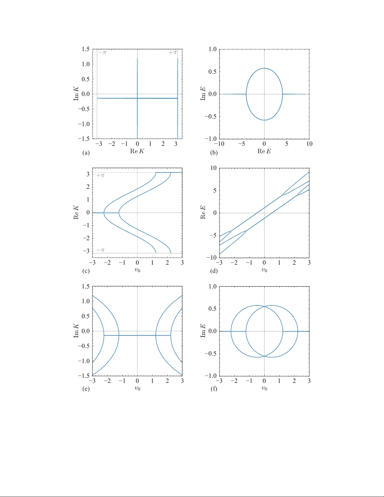
Non-Hermitian Quantum Mechanics of Op en Quantum Systems: Revisiting The One-Bo dy Problem Naomichi Hatano Institute of Industrial Science, The University of T oky o, Kashiw a, Chiba 277-8574, Japan Gonzalo Ordonez Depa rtment of Physics and Astronomy , Butler University , Gallahue Hall, 4600 Sunset Avenue, Indianap olis, Indiana 46208, USA (Dated: F eb rua ry 17, 2026) W e review analyses of op en quan tum systems within the one-bo dy problem. Open quantum systems are systems, possibly complicated but with a ﬁnite num ber of degrees of freedom, to whic h systems, p ossibly with an inﬁnite n um ber of degrees of freedom but simple, are coupled. W e show how non-Hermiticity arises in an op en quantum system with an inﬁnite environment, fo cusing on the one-b o dy problem. One of the reasons for taking the present approac h is that we can solv e the problem completely , making it easier to see the structures of problems inv olving op en quantum systems. W e show that this results in the discov ery of a new complete set, which is one of the main topics of the present article. Another reason for focusing on the one-b ody problem is that the theory p ermits the strong coupling b etw een the system and the environmen t. F or systems with interac- tions, particularly within the environment, the Born-Marko v appro ximation is quite of- ten used, although the dynamics of op en quan tum systems is generally non-Marko vian. Since the Born appro ximation is v alid only in a weak-coupling regime, phenomena that would emerge uniquely in strong-coupling regimes are yet to b e pursued. In the current research landscape, it is v aluable to revisit the one-bo dy problem for op en quantum sys- tems, whic h can b e solved accurately for arbitrary strengths of the system-environmen t couplings. A rigorous understanding of the problem structures in the present approach will b e helpful when w e tackle problems with many-bo dy in teractions. First, we consider potential scattering and directly deﬁne the resonant state as an eigen- state of the Schr¨ odinger equation under the Siegert outgoing b oundary condition. W e show that the resonant eigenstate can hav e a complex energy eigenv alue, even though the Hamiltonian is seemingly Hermitian. W e resolv e common puzzlementss ab out the resonant states, including the app earance of complex eigenv alues and the divergence of the eigenfunctions. In this direct formalism, the non-Hermiticit y of open quantum systems is hidden in the b oundary condition. Second, we introduce the F eshbac h formalism, which eliminates the inﬁnite degrees of freedom of the environmen t and represents its eﬀect as a complex p oten tial. The non- Hermiticity hidden in the direct form ulation manifests as the complexity in the F esh bach formalism. The resulting eﬀectiv e Hamiltonian is explicitly non-Hermitian. By unifying these tw o wa ys of deﬁning resonant states, w e obtain a new complete set of bases for the scattering problem that contains all discrete eigenstates, including resonant states. W e ﬁnally men tion the non-Marko vian dynamics of open quantum systems. In particu- lar, we sho w that the system’s op enness emerges as non-Mark ovianit y in both the short- and long-time regimes. W e emphasize the time-rev ersal symmetry of the dynamics that contin uously connects the past and the future. W e can capture it using the new complete set that we dev elop here. CONTENTS I. Introduction: T arget of the present article 2 II. Resonant states in op en quan tum systems 3 1. Poten tial scattering as an op en quan tum system 3 2. Finding the resonant states using the Siegert b oundary condition 4 3. Resolving puzzlements ab out the resonan t state 8 4. Solutions of the scattering problem for the tight-binding mo del 11 5. Solutions of the resonant states for the tigh t-binding model 12 II I. F esh bach formalism: Reduction to an eﬀective Hamiltonian 15 1. F eshbac h formulation in a tight-binding mo del 15 2. A new complete set inv olving the resonant states 17 2 3. Breaking down quantum dynamics in to the new complete set 19 4. Calculation of the eﬀective Hamiltonian in con tinuous models 23 IV. Non-Marko vian dynamics of op en quan tum systems 26 1. F eshbac h formalism for the time-dep endent Sc hr¨ odinger equation 27 2. Short-time and long-time deviation from the Marko vian decay 28 V. Conclusions 29 Ackno wledgments 30 A. Finding scattering solutions of the p oten tial (5) 30 B. T ransision from a resonant-an ti-resonant pair to a bound-anti-bound pair 31 C. Introduction to the tight-binding model 32 D. Calculation of the Green’s function in Eq. (89) 34 E. Analytic calculations in SubSecs. I II.3 and IV.2 36 1. An algebraic proof of the formula (125) 36 2. Deriv ation of Eq. (126) 37 3. Deriv ation of Eq. (181) 38 F. Introduction to the quantum Zeno eﬀect 38 G. Finding the power la w t − 3 in the long-tome regime 39 References 40 I. INTRODUCTION: T ARGET OF THE PRESENT ARTICLE In this article, we review analyses of open quan tum systems within the one-b o dy problem. Op en quantum systems (see e.g. Refs. (Breuer and Petruccione, 2010; Riv as and Huelga, 2011; V acchini, 2024) for general text- b ooks) are systems, p ossibly complicated but with a ﬁ- nite num b er of degrees of freedom, to whic h systems, p ossibly with an inﬁnite num b er of degrees of freedom but simple, are coupled. W e hereafter refer to the former simply as the system, while to the latter as the en viron- men t; see Fig. 1(a). In this article, we rep eatedly stress that non-Hermiticit y in an open quantum system arises only when the environmen t has an inﬁnite num b er of de- grees of freedom. W e can classify problems in op en quan tum systems in to three categories, dep ending on whether interactions o ccur within the system or in the environmen t. If we assume that there are no in teractions within the system or the en vironment, the problem reduces to a one-bo dy problem and is mostly solv able. When w e assume in ter- actions in the syste m but not in the environmen t, the problem ma y still b e solv able if we can successfully di- agonalize the system Hamiltonian. Finally , if we wan t a heat bath for the environmen t, we would need inter- actions within it as w ell. W e would most lik ely need appro ximations for the third category . system environment V ( x ) x (a) (b) FIG. 1: (a) A schematic view of the system and the en vironmen t of an op en quantum system. The system indicated b y a small circle is em b edded in the en vironmen t indicated by a big circle, with a coupling b et ween them indicated by a solid red curve. (b) In the problem of p oten tial scattering, the p oten tial area is iden tiﬁed as the system, while the rest, ﬂat space is iden tiﬁed as the en vironmen t. W e here focus on the problem in the ﬁrst category . One of the reasons for taking the present approach is that we can solv e the problem completely , which mak es it easy to see the structures of problems in v olving op en quantum systems. Indeed, this results in the discov ery of a new complete set (Hatano and Ordonez, 2014), which we will review b elo w. Another reason is that the theory p ermits the strong coupling b etw een the system and the environmen t. F or the problems in the third category in particu- lar, b ecause of v arious diﬃculties in solving them, the Gorini-Kossak o wski-Sudarshan-Lindblad (GKSL) equa- tion (Gorini et al. , 1976; Lindblad, 1976) after Born- Mark o v approximations (Breuer and Petruccione, 2010) is quite often used, although the dynamics of op en quan- tum systems is generally non-Mark ovian. Since this ap- pro ximation is v alid only in a w eak-coupling regime, phe- nomena that would emerge uniquely in strong-coupling regimes are y et to b e pursued. In the current research landscap e, it is v aluable to re- visit the one-b ody problem for op en quan tum systems, whic h can b e solved accurately for arbitrary strengths of the system-en vironment couplings. A rigorous under- standing of the problem structures in the presen t ap- proac h will b e helpful when we tac kle problems in higher categories. The problem of open quantum systems dates back to 3 Gamo w in 1928 (Gamow, 1928), when he introduced a non-Hermitian comp onen t to the Hamiltonian to explain alpha deca y . The theory was then developed primarily in n uclear ph ysics (Hum blet, 1962, 1964a,b; Humblet and Rosenfeld, 1961; Jeukenne, 1964; Mahaux, 1965; Rosen- feld, 1961, 1965) and related mathematical ph ysics (Cou- teur and P eierls, 1960; Hokky o, 1965; P eierls, 1959; Romo, 1968; Zel’dovic h, 1960), although it was not re- ferred to as an op en quantum system at the time. There are t wo storylines. On one hand, the deﬁnition of the resonant state with a complex energy eigenv alue w as developed, particularly by Siegert in 1939 (Siegert, 1939). The resonant state w as then deﬁned as an eigen- state of the Sc hr¨ odinger equation under a sp eciﬁc bound- ary condition. On the other hand, F eshbac h in 1958 (F es- h bac h, 1958, 1962) justiﬁed the in tro duction of a non- Hermitian comp onen t to the Hamiltonian as he elimi- nated the comp onen ts of the environmen tal inﬁnite de- grees of freedom. In the present article, we provide an ov erview of these results. W e unify the tw o storylines and, as a conse- quence, ﬁnd a new complete set of bases for the scattering problem based on resonan t states. Accordingly , w e deﬁne resonan t states in tw o w ays. First, in Sec. I I, we consider p oten tial scattering and di- rectly deﬁne the resonant state as an eigenstate of the Sc hr¨ odinger equation under the Siegert b oundary condi- tion. W e show that the resonant eigenstate can hav e a complex energy eigen v alue, even though the Hamiltonian is seemingly Hermitian. In this direct formalism, the non- Hermiticit y of the op en quantum system is hidden in the b oundary condition. Second, in Sec. I II, we introduce the F eshbac h formal- ism, with whic h we eliminate the inﬁnite degrees of free- dom of the environmen t, and represent its eﬀect as a com- plex p oten tial. The non-Hermiticity hidden in the direct form ulation manifests as the complexity in the F esh bac h formalism. The resulting eﬀective Hamiltonian is explic- itly non-Hermitian. W e then men tion the non-Mark ovian dynamics of open quan tum systems in Sec. IV b efore summarizing the ar- ticle in Sec. V. In particular, w e show that the system’s op enness emerges as non-Mark o vianity in both the short- and long-time regimes. W e emphasize the time-reversal symmetry of the dynamics around t = 0, which w e can capture using the new complete set that w e develop in Sec. I II. I I. RESONANT ST A TES IN OPEN QUANTUM SYSTEMS As schematically shown in Fig. 1(b), p oten tial scatter- ing is one of the simplest nontrivial v ersions of the op en quan tum system. W e iden tify the p oten tial area of a ﬁ- nite range as the system and the ﬂat outer space that extends inﬁnitely as the environmen t. In this section, we sho w the app earance of resonan t eigenstates with com- plex energy eigen v alues, indicating the problem’s non- Hermiticit y . W e primarily work in contin uous space, but w e also translate it into a lattice problem to provide a more straigh tforw ard explanation in the next Sec. I II. 1. Potential scattering as an op en quantum system Let us consider the problem of p oten tial scattering with the standard time-indep endent Schr¨ odinger equa- tion in one dimension:  − ℏ 2 2 m d 2 d x 2 + V ( x )  ψ ( x ) = E ψ ( x ) . (1) Here and hereafter, w e assume that the potential function V ( x ) is real and its supp ort is compact; it takes nonzero real v alues only within a ﬁnite range: V ( x ) ≡ 0 for | x | > ℓ, (2) where ℓ is a ﬁnite p ositiv e num b er. In other words, we exclude p oten tials of inﬁnite range. At this momen t, we do not kno w ho w we can extend the analyses below to the case of inﬁnite-range potentials, suc h as the Coulomb p oten tial. In this and the following subsections, we will deﬁne the resonan t state, whic h indeed has a complex energy eigen v alue, as a solution of the Sc hr¨ odinger equation (1) under the b oundary condition of out-going wa ves only: ψ ( x ) ∝ e i K | x | for | x | > ℓ, (3) where E = ( ℏ K ) 2 / (2 m ). This was ﬁrst proposed b y Siegert in 1939 (Siegert, 1939); hence, w e refer to it as the Siegert boundary condition. W e explain the rationale for this deﬁnition of the resonan t state b elo w. Note that we will show b elow that K and E can b e complex under the Siegert boundary condition. Here and hereafter, we use the capital K to indicate that the v alue can b e complex, whereas we use the low ercase k to in- dicate that it is either real or the real part of K . F or Re K > 0, the b oundary condition (3) means that the w a ve is righ t-going for x > ℓ and left-going for x < − ℓ . W e will refer to such an eigenstate as the resonan t state. F or Re K < 0, the b oundary condition (3) means that the w a ve is left-going for x > ℓ and righ t-going for x < − ℓ . W e will refer to such an eigenstate as the anti-resonan t state. W e begin our explanation with the usual scattering problem. W e assume an incident wa ve on the left of the p oten tial, a reﬂection w av e on the left, and a transmission w a ve on the righ t: ψ ( x ) = ( A e +i kx + B e − i kx for x < − ℓ, C e +i kx for x > + ℓ. (4) 4 V ( x ) x (a) V 1 V 1 − V 0 V ( x ) x (b) 0 FIG. 2: (a) The p oten tial of three delta functions in Eq. (5). (b) A schematic p oten tial we hav e in mind. W e then deriv e the relations among the amplitudes A , B , and C from the connection conditions. F or example, let us analyze the case of a set of delta p oten tials V ( x ) = − V 0 δ ( x ) + V 1 ( δ ( x + ℓ ) + δ ( x − ℓ )) , (5) where V 0 > 0 and V 1 > 0, as in Fig. 2(a), which w ould mimic the situation in Fig. 2(b), which would fur- ther mimic a shell-mo del p oten tial in nuclear and atomic ph ysics. W e present details of the calculation in App. A. W e obtain the transmission amplitude in the form t amp := C A = 1 T 11 , (6) where the (1 , 1) comp onen t of the transfer matrix, T 11 , is given by Eq. (A8), and the transmission co eﬃcien t in the form T :=     C A     2 = 1 | T 11 | 2 . (7) W e will plot this along with the resonance p oles b elow in Figs. 4 and 6. In the standard textbo ok of quan tum mec hanics, a res- onan t state is often deﬁned as a p ole of the transmission co eﬃcien t. The expression (6) then implies that the p ole of the transmission amplitude t amp is given b y the zero of the amplitude A and that the wa ve function that cor- resp onds to the pole is found b y putting A to zero from the very beginning in Eq. (4). This is the rationale of setting the b oundary condition in the form (3) to ﬁnd the resonance p oles. 2. Finding the resonant states using the Siegert b oundary condition Setting the Siegert b oundary condition ψ ( x ) = ( B e − i K x for x < − ℓ, C e +i K x for x > + ℓ (8) mak es the calculation of the resonance p oles quite easier than the one presen ted in App. A. One point to note here is the reduction of the n um b er of unknown v ariables. In solving the scattering problem, as in the previous Subsec. II.1, we ha ve the unknown v ariables k , A , B , and C in Eq. (4) as w ell as J , M , F , and G in Eq. (A1). Since w e need only the ratios of the amplitudes, the num b er of unkno wn v ariables is seven. T o determine them, we ha ve six conditions given in Eq. (A2), and hence there is one v ariable that w e cannot determine. In fact, we make the w a ve num b er k of the incident wa ve a control parameter in solving the scattering problem. On the other hand, we set A = 0 in the Siegert b ound- ary condition (8), thereby reducing the n umber of un- kno wn v ariables by one. W e now hav e six unknown v ari- ables to be determined by six conditions (A2). This al- lo ws us to ﬁnd discrete solutions to K , whic h we will sho w in the presen t subsection. Since the potential function (5) is an even function, w e can no w classify the resonant states of the form (8) in to those with ev en and o dd parities. This simpliﬁes the computation considerably , as w e show b elo w. Let us ﬁrst consider the simple case of V 0 = 0, which lea v es us only the positive delta p eaks at x = ± ℓ (Hatano et al. , 2008). In this case, we can generally assume the follo wing with the Siegert b oundary condition (8): ψ ( x ) =      B e − i K x for x < − ℓ, F e +i K x ± G e − i K x for − ℓ ≤ x ≤ ℓ, C e +i K x for x > + ℓ, (9) but for a ﬁxed parit y , we can further assume B = ± C , G = ± F , (10) where the upper sign corresp onds to ev en-parity solutions and the low er sign to o dd-parit y ones throughout the presen t subsection. Since we need only the ratios of the amplitudes, the unknown v ariables are reduced to the follo wing t w o: K and F /C . W e determine them with the following t w o connection conditions: ψ (+ ℓ − ϵ ) = ψ (+ ℓ + ϵ ) , (11a) ψ ′ (+ ℓ − ϵ ) = ψ ′ (+ ℓ + ϵ ) − 2 v 1 ψ (+ ℓ ) , (11b) where v 1 := mV 1 ℏ 2 . (12) 5 The second condition (11b) is found by integrating the Sc hr¨ odinger equation o ver an inﬁnitesimally narro w re- gion [+ ℓ − ϵ, + ℓ + ϵ ]. Using Eq. (9) in Eq. (11), w e obtain F  e +i K ℓ ± e − i K ℓ  = C e +i K ℓ (13a) i K F  e +i K ℓ ∓ e − i K ℓ  = i C K e +i K ℓ − 2 v 1 C e +i K ℓ (13b) Multiplying both sides b y e − i K ℓ and inserting C on the righ t-hand side of the ﬁrst equation into that of the sec- ond one, w e end up with e 2i K ℓ = ∓  1 − i K v 1  , (14) In fact, these equations are found from setting T 11 in Eq. (A8) to zero with v 0 := mV 0 / ℏ 2 = 0, as in T 11 = 1 k 2 " −  1 − i k v 1  2 + e 4i kℓ # = 0 , (15) although w e do not immediately know the parit y of the solutions from it. W riting K = k + i κ and introducing the dimensionless v ariables ξ := k ℓ , η := κℓ and α 1 := ℓv 1 , w e can tranform Eq. (14) in to e 2i ξ − 2 η = ∓  1 − i ξ − η α 1  . (16) T aking the real and imaginary parts of b oth sides of Eq. (16), w e ha v e e − 2 η cos(2 ξ ) = ∓  1 + η α 1  , (17a) e − 2 η sin(2 ξ ) = ± ξ α 1 . (17b) whic h w e can transform in to η = − 1 2 ln  ± ξ α 1 csc(2 ξ )  , (18a) η = − ξ cot(2 ξ ) − α 1 . (18b) W e can ﬁnd the solutions { ξ n , η n } as the crossing p oints of the t w o curves, as shown in Fig. 3; note that the cross- ing points also exist on the negative side of ξ symmet- rically b ecause the right-hand sides of b oth of Eq. (18) are even functions of ξ . W e can n umerically ﬁnd accu- rate solutions using the Newton-Raphson metho d, with an initial guess pro vided by a rough estimate that w e read oﬀ from Fig. 3 (Hatano et al. , 2008). Figure 4 shows go od agreemen t b et ween the transmis- sion coeﬃcient (7) with v 0 = 0 and the locations of the resonance p oles. F or each resonance eigen-wa ve-n umber, the real part giv es the peak lo cation, and the imaginary part roughly giv es the p eak width. 0.0 −1.0 −1.2 −0.8 −0.6 −0.4 −0.2 0 2 4 6 8 FIG. 3: Plots of the tw o curves Eq. (18a) (dashed blue curv es for ev en so lutions and dot-dashed red curves for o dd solutions) and Eq. (18b) (solid black curves). The v ertical brok en gray lines indicate multiples of π / 2 on the ξ axis. The crossing p oin ts indicated by crosses with green squares indicate resonan t states of ev en parit y and those indicated b y crosses with green circles indicate resonan t states of o dd parity . The example is giv en for α 1 = 1 with V 0 = 0. 0 0.0 0.2 0.4 0.6 0.8 1.0 2 4 6 8 0.0 −0.2 −0.4 −0.6 −0.8 −1.0 FIG. 4: The transmission co eﬃcien t T (blue curv e) for v 0 = 0 and the lo cations { ξ n , η n } of the resonance p oles, whic h are the same as the ones in Fig. 3. F or the v alues of the former and the latter, see the left and right v ertical axes, resp ectiv ely . The example is given for α 1 = 1 with V 0 = 0. In fact, this agreement is not alwa ys true. W e can conﬁrm that the real w a v e num b er k ℓ cot(2 k ℓ ) + ℓv 1 = 0 , (19) whic h we obtain b y setting η to zero in Eq. (18b), giv es the p oin t of p erfect transmission T = 1 / | T 11 | 2 = 1. This means that, in this particular case, the agreement is go od for a small v alue of η . W e will see in the next example that this agreemen t breaks. T o see it, we introduce a p ositiv e v alue of V 0 . This ac- tually do es not aﬀect the solutions of o dd parit y , b ecause 6 they do not couple to the p otential at the origin. F or the solutions of ev en parit y , we replace Eq. (18) with ψ ( x ) =          C e − i K x for x < − ℓ, F e − i K x + G e +i K x for − ℓ ≤ x ≤ 0 , F e +i K x + G e − i K x for 0 ≤ x ≤ + ℓ, C e +i K x for x > + ℓ. (20) The tw o connection conditions (11) are also supple- men ted b y ψ ′ ( − ϵ ) = ψ ′ (+ ϵ ) + 2 v 0 ψ (0) , (11c) where v 0 := mV 0 ℏ 2 . (21) With these three connection conditions (11a), (11b), and (11c), w e ﬁx the ratios F /C and G/C along with the p oin t sp ectra of K . Using the form (20) in the three connection conditions, w e ha v e  F e +i K ℓ + G e − i K ℓ  = C e +i K ℓ (22a) i K  F e +i K ℓ − G e − i K ℓ  = i C K e +i K ℓ − 2 v 1 C e +i K ℓ , (22b) − i K ( F − G ) = i K ( F − G ) + 2 v 0 ( F + G ) , (22c) Eliminating C from the ﬁrst tw o equations, we hav e i K  F e 2i K ℓ − G  = (i K − 2 v 1 )  F e 2i K ℓ + G  , (23) or v 1 e 2i K ℓ F = (i K − v 1 ) G. (24) F rom the third condition (22c), on the other hand, we ha v e (i K + v 0 ) F = (i K − v 0 ) G. (25) Com bining Eqs. (24) and (25), w e obtain (i K − v 0 ) e 2i K ℓ = − (i K + v 0 )  1 − i K v 1  , (26) Expressing this equation in terms of the dimensionless quan tities, w e hav e (i ξ − η − α 0 ) e 2i ξ − 2 η = − (i ξ − η + α 0 )  1 − i ξ − η α 1  , (27) where α 0 = v 0 ℓ . This equation is more complicated than in the case of v 0 = 0 in Eq. (16), and it seems imp ossible to ﬁnd the explicit equations for the real and imaginary parts of the form (18). In such a case, we propose the following approac h to obtain numerically accurate solutions. W e ﬁrst mak e a densit y plot of the follo wing function in the complex K plane: f ( ξ , η ) := log     (i ξ − η − α 0 ) e 2i ξ − 2 η + (i ξ − η + α 0 )  1 − i ξ − η α 1      . (28) Then the solutions of Eq. (27) should appear as dark sp ots that represen t negative inﬁnit y , as is exempliﬁed in Fig. 5. W e can then use the Newton-Raphson metho d in tw o dimensions to obtain numerically accurate solu- tions { ξ n , η n } , equating the real and imaginary parts of Eq. (27), with an initial guess set as a rough estimate that w e read oﬀ from Fig. 5. W e plot the transmission co eﬃcient (7) and the loca- tions of the resonance p oles in Fig. 6 for V 0 > 0. W e note that there is only one broad resonance p eak for a pair of o dd-parit y and ev en-parity resonance p oles in this case; see App. B for more details regarding the transition from Fig. 4 to Fig. 6. The introduction of V 0 breaks the go o d agreement b e- t w e en the p ole locations and the resonance p eaks. This implies that only chec king the resonance p eaks may miss hidden resonance p oles. Note that resonance p oles are more ph ysical en tities than resonance p eaks; unstable n uclides with ﬁnite lifetimes, such as nihonium (Morita et al. , 2012), are nothing but resonant states. This un- derscores the imp ortance of pursuing the resonant states with complex eigen v alues. T o summarize the calculations for the example ab o ve, w e generally hav e the distribution of p oin t sp ectra in the complex K plane, including resonan t states, as shown in Fig. 7(a). The states on the positive imaginary axis are in fact b ound states, whic h we can realize by putting K = i κ with κ > 0 into Eq. (8). There is a contin- uum of scattering states ov er the entire real axis of k . R. Newton (Newton, 1960, 1982) prov ed that all bound states together with the entire contin uum of the scatter- ing states constitute a complete set of the Hilb ert space. 7 0 0 5 2 10 4 −5 −2 −10 −4 FIG. 5: The density plot of the function (28). The blac k sp ots indicate negative inﬁnity . The example is giv en for α 0 = 3 and α 1 = 1. 0 0.0 0.2 0.4 0.6 0.8 1.0 2 4 6 8 10 12 0.0 −2.5 −2.0 −1.5 −0.5 −1.0 FIG. 6: The transmission co eﬃcien t T (blue curv e) and the lo cations { ξ n , η n } of the resonance p oles of even parit y (blac k crosses) as well as the unchanged p oles of o dd parity (gray crosses). F or the v alues of T and the lo cation of b oth p oles, see the left and right vertical axes, resp ectiv ely . The example is given for α 0 = 3 and α 1 = 1. The states below the real axis of k are therefore outside the Hilb ert space. Indeed, these states are not normal- izable, as can b e seen b y taking K = i κ with κ < 0 in Eq. (8); the eigenstates diverge exp onen tially on b oth sides of the space as x → ±∞ . This ma y b e why the res- onan t states are often called unph ysical, but w e will show in the next Subsec. I I.3 that w e need this spatial div er- gence for probability conserv ation. (W e refer the readers to a textbo ok (Moisey ev, 2011) and a recen t review (My o and Kat¯ o, 2020) for a metho d called complex scaling for making the divergen t eigenfunctions conv ergent.) The states in the fourth quadrant of the complex K plane are called the resonant states, whereas those in the third quadran t are called the an ti-resonant states. W e will also sho w in the next Subsec. II.3 that ev ery resonant state and its corresp onding anti-resonan t state form a pair, Bound states Scattering states Anti-bound states Resonant states Anti-resonant states Bound states Scattering states Anti-bound states Resonant states Anti-resonant states (a) (b) First Riemann sheet Second Riemann sheet FIG. 7: Schematic plots of the distributions of the eigen v alues (a) in the complex K plane and (b) in the complex E plane with tw o Riemann sheets. with the tw o states b eing time-reversed. The states on the negativ e real axis are called an ti-b ound states. Mo ving o v er to the complex E plane, we ha v e tw o Rie- mann sheets corresp onding to the upper and lo w er half parts of the complex K plane, b ecause of the dispersion relation E ∝ K 2 . The t w o sheets are connected on the branc h cut indicated b y a w avy line in Fig. 7(b). The ﬁrst Riemann sheet of the complex E plane has 8 all the b ound states on the negative real axis and all the scattering states on the p ositive real axis. All states that b elong to R. Newton’s complete (Newton, 1960, 1982) set are therefore lo cated in the ﬁrst Riemann sheet. The second Riemann sheet of the complex E plane, on the other hand, has resonant states in the low er half- plane, an ti-resonant states in the upper half-plane, and an ti-b ound states on the negative real axis. B. Simon (Si- mon, 2000) prov ed a sp eciﬁc arrangemen t of the b ound and anti-bound states for a semi-inﬁnite space, but no arrangemen t is known for the inﬁnite space, as far as we are a w are. 3. Resolving puzzlements ab out the resonant state A t this point, readers may hav e sev eral questions about the ph ysical relev ance of states with complex energy eigen v alues and their div erging eigenfunctions. W e ﬁrst presen t physical in terpretations of the resonant and anti- resonan t states, and then address p ossible questions. Consider the Siegert boundary condition (8) with the time-dep enden t part: Ψ n ( x, t ) = e − i E n t/ ℏ × ( B e − i K n x for x < − ℓ, C e +i K n x for x > + ℓ, (29) where n denotes eac h resonant or anti-resonan t eigen- state. In Fig. 7, we note Re K n > 0 and Im E n < 0 for the resonant states. This means, as schematically shown in Fig. 8(a), that the probability ﬂux escap es from the cen tral p otential area (red horizontal arrows), and corre- sp ondingly the probability in the cen tral area deca ys in time (green v ertical arro w). On the other hand, we hav e Re K n < 0 and Im E n > 0 for the anti-resonan t states. This means, as schematically sho wn in Fig. 8(b), that the probabilit y ﬂux is injected in to the central area (red horizontal arrows), and conse- quen tly the probabilit y there grows in time (green ver- tical arrow). (Note, how ever, that eac h of the resonan t and anti-resonan t states never exists as a single state; it only exists as a comp onen t of a superimp osed state, as w e show in the next Sec . I II. They either decay or grow from the inﬁnite past to the inﬁnite future, which should not happ en in reality .) W e now provide answers to the following ques- tions (Hatano, 2021): (i) Why can the Schr¨ odinger equation (1) with the “Hermitian” Hamiltonian ha ve eigenstates with complex energy eigen v alues? (ii) How can we understand the spatially diverging w a ve functions? (iii) Why can the time-reversal symmetric eigen v alue problem (1) ha ve eigenstates that break time- rev ersal symmetry? x (a) x (b) FIG. 8: Schematic views of (a) the resonant state and (b) the an ti-resonan t state. The answer to the question (i) will also lead to the answ er to the question (ii). Let us remember ho w w e pro v ed the “Hermiticity” of the Hamiltonian ˆ H = − ℏ 2 2 m d 2 d x 2 + V ( x ) . (30) If we can pro ve that the expectation v alue ⟨ ψ | ˆ H | ψ ⟩ is real for an “arbitrary” function | ψ ⟩ , then the Hamiltonian ˆ H is a Hermitian operator. Since we assume the potential V ( x ) is real, and its supp ort is compact, ⟨ ψ | V | ψ ⟩ = Z ∞ ∞ ψ ( x ) ∗ V ( x ) ψ ( x )d x (31) should be real for an arbitrary function ψ ( x ) whic h is not singular at least within the supp ort of the p oten tial. The issue arises from the exp ectation v alue of the ki- netic term. W e ﬁrst consider its exp ectation v alue under the integration ov er a ﬁnite range [ − L, L ], where L > ℓ , and chec k whether we can take the limit L → ∞ . F ol- lo wing the strategy , w e deﬁne, for an “arbitrary” function ψ ( x ), ⟨ ψ |  − h 2 2 m d 2 d x 2  | ψ ⟩ L := − h 2 2 m Z L − L ψ ( x ) ∗ d 2 d x 2 ψ ( x )d x. (32) After partial in tegration, we can transform the righ t- hand side of Eq. (32) as in − ℏ 2 2 m  ψ ( x ) ∗ d d x ψ ( x )  + L x = − L + ℏ 2 2 m Z L − L     d d x ψ ( x )     2 d x. (33) 9 The second term of Eq. (33) has no imaginary part even in the limit of inﬁnite L , but the ﬁrst term is generally complex. In the elementary level of quantum mechanics, readers might hav e b een told that the ﬁrst term w ould v anish if the function ψ ( x ) v anishes quic kly enough in the limit L → ∞ , b eing square-in tegrable, and hence Eq. (32) would b e real, and the Hamiltonian operator is Hermitian. Therefore, all of its energy eigenv alues m ust b e real. In fact, this argument means that the proof of the Hermiticit y is v alid only when the “arbitrary” function ψ ( x ) is chosen from a speciﬁc functional space of func- tions that v anish quickly enough in the limit L → ∞ , and the Hamiltonian (30) is Hermitian only within such a functional space. The Hamiltonian, or more sp ecif- ically the kinetic term − ( ℏ 2 / 2 m ) d 2  d x 2 , can b e non- Hermitian outside such a functional space. In other w ords, whether the Hamiltonian (30) is Hermitian or non-Hermitian could not b e determined without sp eci- fying the functional space that w e w ork in. Indeed, in explaining the eigen v alue distribution in the complex K plane in Fig. 7(a), we stressed that the states in the lo w er half plane of the complex K plane diverge exp onen tially on b oth sides of x → ±∞ . Hence, the ﬁrst term of Eq. (33) do es not v anish in the limit L → ∞ for the resonant and an ti-resonant states. The Hamil- tonian ˆ H can be non-Hermitian in the functional space of these eigenstates, and therefore they can legitimately ha v e complex energy eigenv alues. This is the answ er to the question (i). It also underscores that resonant states with complex eigen v alues can app ear only when the en vironmental sys- tem extends to inﬁnity . Indeed, we would not b e able to set the Siegert b oundary condition (29) if the envi- ronmen tal system is of a ﬁnite size; the outgoing w a v es w ould b ounce back to the system. As w e emphasized at the beginning of the article, the non-Hermiticity of the op en quantum system arises only when the environmen- tal system is inﬁnite. As we men tioned earlier, the spatial div ergence of its w a ve function may b e why the resonan t state is often called unphysical. W e now sho w that the spatial diver- gence is, in fact, necessary for probabilit y conserv ation. W e analyze the imaginary part of the exp ectation v alue ⟨ Ψ | ˆ H | Ψ ⟩ L , where we let | Ψ ⟩ contain the time-dep enden t factor e − i E t/ ℏ . The imaginary part of the element comes only from the ﬁrst term of Eq. (33), and hence Im ⟨ Ψ | ˆ H | Ψ ⟩ L = − h 2 2 m Im  Ψ( x, t ) ∗ d d x Ψ( x, t )  + L x = − L . (34) The left-hand side of Eq. (34) is transformed as follo ws. Consider the time-dep enden t Schr¨ odinger equation i ℏ d d t Ψ( x, t ) = ˆ H Ψ( x, t ) (35) and its complex conjugate − i ℏ d d t Ψ( x, t ) ∗ = ˆ H Ψ( x, t ) ∗ . (36) Therefore, w e ha v e i ℏ d d t ⟨ Ψ | Ψ ⟩ L = i ℏ Z L − L d x  d d t Ψ( x, t ) ∗  Ψ( x, t ) + Ψ( x, t ) ∗  d d t Ψ( x, t )  (37a) = Z L − L d x h −  ˆ H Ψ( x, t ) ∗  Ψ( x, t ) + Ψ( x, t ) ∗  ˆ H Ψ( x, t ) i (37b) =  ⟨ Ψ | ˆ H | Ψ ⟩ L − ⟨ Ψ | ˆ H | Ψ ⟩ L ∗  = 2i Im ⟨ Ψ | ˆ H | Ψ ⟩ L (37c) The right-hand side of Eq. (34), on the other hand, is giv en in terms of the momen tum operator ˆ p = ( ℏ / i) d/d x as in − ℏ 2 m Re (Ψ( L, t ) ∗ ˆ p Ψ( L, t ) − Ψ( − L, t ) ∗ ˆ p Ψ( − L, t )) (38) This gives, apart from the co eﬃcien t, the momentum ﬂux going out from the right b oundary x = L and from the left b oundary x = − L , as is sc hematically sho wn in Fig. 8(a). Combining Eqs. (37) and (38), we realize that Eq. (34) yields an equation of contin uit y of the probabil- it y densit y , d d t ⟨ Ψ | Ψ ⟩ L = − ℏ m Re (Ψ( L, t ) ∗ ˆ p Ψ( L, t ) − Ψ( − L, t ) ∗ ˆ p Ψ( − L, t )) , (39) whic h implies the probabilit y conserv ation. Let us explicitly demonstrate probability conserv ation for eac h resonan t state as follows (Hatano et al. , 2009). 10 x FIG. 9: The exp onen tial decrease of the wa ve function o v er time due to Im E n < 0 is cance led out by the exp onen tial increase of the wa ve function due to Im K n < 0 when we expand the in tegral range at the sp eed of the ﬂux. W e deﬁne the probabilit y in the following form: P n ( t ) := ⟨ Ψ n | Ψ n ⟩ L n ( t ) (40a) = Z L n ( t ) − L n ( t ) Ψ n ( x, t ) ∗ Ψ n ( x, t )d x. (40b) Here Ψ n ( x, t ) is one sp eciﬁc resonant eigenstate of the form (29) and L ( t ) := Re ℏ K n m t + ℓ (41) for t > 0, where ℏ K n /m is the phase velocity deﬁned by d E n /d p = d E ( K n )/d( ℏ K n ) . The idea b ehind this deﬁnition is shown in Fig. 9. The sc hematic view of Fig. 8(a) suggests that the temp oral de- crease of the probabilit y must be equal to the probabilit y ﬂuxes going out of the p oten tial area. The probability , in- tegrated o ver a ﬁxed range, w ould decrease exp onen tially o v er time. In Eq. (40), we c hase the escaping ﬂuxes b y expanding the in tegral range at the sp eed of the ﬂuxes. W e will indeed ﬁnd that the probability (40) is time- indep enden t. In other words, the exp onen tial decrease in time due to Im E < 0 balances with the exp onen tial increase in space due to Im K < 0. This implies that the exp onen tial divergence of the wa ve function of the resonan t state is not unphysical; On the contrary , it is essen tial in probabilit y conserv ation. W e now prov e that the time deriv ative of the proba- bilit y (40) v anishes. The time deriv ative of P n ( t ) con- sists of t wo terms: the time deriv ative of the in tegrand Ψ n ( x, t ) ∗ Ψ n ( x, t ) and the time deriv ative of the integral range ± L ( t ). The calculation of the former is similar to Eq. (37), and w e obtain Z L n ( t ) − L n ( t ) d d t (Ψ n ( x, t ) ∗ Ψ n ( x, t ))d x = 2 ℏ Im ⟨ Ψ n | ˆ H | Ψ n ⟩ L ( t ) = − h m Im  Ψ n ( x, t ) ∗ d d x Ψ n ( x, t )  + L n ( t ) x = − L n ( t ) , (42) where w e used Eq. (34) for the second equalit y . On the other hand, the calculation that inv olves the time deriv ativ e of ± L ( t ) is given by d L n ( t ) d t  | Ψ n ( L n ( t ) , t ) | 2 + | Ψ n ( − L n ( t ) , t ) | 2  (43) This quan tity is related to the righ t-hand side of Eq. (34) through Eq. (29). Since L > ℓ , we hav e d d x Ψ n ( x, t ) = Ψ n ( x, t ) × ( − i K n for x = − L, +i K n for x = + L, (44) and hence ℏ 2 2 m Im  Ψ( x, t ) ∗ d d x Ψ( x, t )  + L n ( t ) x = − L n ( t ) = ℏ 2 2 m Im (i K n )  | Ψ(+ L n ( t ) , t ) | 2 + | Ψ( − L n ( t ) , t ) | 2  (45a) = Re ℏ 2 K n 2 m  | Ψ(+ L n ( t ) , t ) | 2 + | Ψ( − L n ( t ) , t ) | 2  . (45b) Therefore, w e ﬁnd d L n ( t ) d t  | Ψ n ( L n ( t ) , t ) | 2 + | Ψ n ( − L n ( t ) , t ) | 2  = ℏ m Im  Ψ( x, t ) ∗ d d x Ψ( x, t )  + L n ( t ) x = − L n ( t ) . (46) This equation exactly cancels out Eq. (42), and hence we ﬁnd d P n ( t )/d t ≡ 0 for the probability (40). The quantit y in Eq. (42) decreases exponentially ov er time, whereas the quan tity in Eq. (46) increases exp onen- tially o ver time because of the spatial divergence of the w a ve function. This is why the probability (40) is con- serv ed. If there were no spatial divergence of the wa ve function of the resonan t state, the probability would not b e conserved, which would b e unph ysical. This is the answ er to the question (ii). A more physical answ er is as follows. F or example, con- sider a quan tum dot connected to electro des. A quan tum dot can harb or Coulom b interactions, whereas electro des conﬁned to tw o-dimensional b oundaries betw een tw o dif- feren t semiconductors can b e nearly free. Hence, this is a t ypical situation of the op en quan tum system. The n um b er of electrons in the quan tum dot is microscopic, whereas the num b er of electrons in the electro des can b e macroscopic, on the order of Av ogadro’s n um b er. It is then plausible to observe exp onen tial growth as we mov e from the quan tum dot tow ards the electro des ov er a rel- ativ ely large distance. The question (iii) is form ulated as follo ws. The time- rev ersal operation ˆ T in quan tum mec hanics not only puts t → − t but also takes the complex conjugation i → − i. Since the Hamiltonian of the Schr¨ odinger equation (1) is 11 real and time-indep enden t, it comm utes with the time- rev ersal op eration: [ ˆ H , ˆ T ] = 0 . (47) This app ears to indicate that the Hamiltonian and the time-rev ersal op eration share the eigenstates, and hence all the eigenstates m ust be tak en to be time-rev ersal sym- metric. This is, ho wev er, not true; we saw in Fig. 8 that the resonant states deca y in time while the anti-resonan t states gro w in time, both of which break the time-rev ersal symmetry . The origin of the seeming contradiction is the fact that the time-rev ersal op eration ˆ T is not a linear operator but an anti-linear one. Supp ose that an eigenstate | ψ n ⟩ of the Hamiltonian ˆ H has an energy eigen v alue E n : ˆ H | ψ n ⟩ = E n | ψ n ⟩ . (48) Op erating ˆ T on b oth sides from the left, we hav e ˆ T ˆ H | ψ n ⟩ = ˆ T E n | ψ n ⟩ . (49) On the left-hand side, we can comm ute ˆ T and ˆ H with eac h other, but on the right-hand side, ˆ T and E n do not generally comm ute with eac h other. What results in is ˆ H ˆ T | ψ n ⟩ = E n ∗ ˆ T | ψ n ⟩ , (50) b ecause of the complex-conjugate op eration of ˆ T . W e therefore hav e tw o cases. If E n is a real energy eigen v alue, Eq. (50) reduces to ˆ H  ˆ T | ψ n ⟩  = E n  ˆ T | ψ n ⟩  . (51) This means that ˆ T | ψ n ⟩ is also an eigenstate of the Hamil- tonian ˆ H with the same energy eigenv alue E n , and hence, if we assume no degeneracy , ˆ T | ψ n ⟩ must b e prop ortional to | ψ n ⟩ and the prop ortionalit y constan t is the eigen v alue of the op erator ˆ T for the eigenstate | ψ n ⟩ . It also means that the state | ψ n ⟩ is time-reversal symmetric. This is the case for the b ound and anti-bound states in Fig. 7. If E n is a complex energy eigen v alue, on the other hand, Eq. (50) indicates that for the eigenstate | ψ n ⟩ , there is alwa ys a partner ˆ T | ψ n ⟩ with the energy eigen- v alue E n ∗ . This relation is precisely what we sa w in Fig. 7(b) b etw een the resonan t and anti-resonan t states. The whole system of the eigenstates conserv es the time- rev ersal symmetry of the Hamiltonian ˆ H . Nonetheless, eac h eigenstate can break the time-reversal symmetry be- cause ˆ T is not a linear op erator. This is the answer to question (iii). 4. Solutions of the scattering p roblem for the tight-binding mo del W e hereafter use the tight-binding model to discuss the resonance poles. (F or readers unfamiliar with the tight- binding mo del, we pro vide a brief introduction to it from x … … 0 FIG. 10: A schematic view of the tight-binding Hamiltonian (52). t w o p ersp ectiv es in App. C.) The tight-binding mo del has only a ﬁnite num b er of p oles, and hence is muc h more tractable than the case of contin uum space, which has a coun tably inﬁnite num b er of p oles. The tractability of the tight-binding mo del lets us discov er a new complete set of bases for scattering problems, whic h is the main topic of Sec. I I I. F or introductory purp oses, we here for- m ulate the scattering problem in the tight-binding mo del, stressing that the wa y to solve it appears to b e diﬀerent from the case of the contin uum space but is essen tially the same. Let us consider the p otential-scattering problem of the follo wing sp eciﬁc Hamiltonian of the tigh t-binding mo del, for example: ˆ H = − W ∞ X n = −∞ n  = − 1 , 0 , 1 ( | n + 1 ⟩ ⟨ n | + | n ⟩ ⟨ n + 1 | ) − W 1 1 X n = − 1 ( | n + 1 ⟩ ⟨ n | + | n ⟩ ⟨ n + 1 | ) + V 0 ( | 0 ⟩ ⟨ 0 | + | 1 ⟩ ⟨ 1 | ) , (52) where W > 0 and W 1 > 0; see Fig, 10. Let us ﬁrst show how to solve the eigenv alue equation for the Hamiltonian (52). Each comp onen t of the eigen- v alue equation reads ⟨ n | ˆ H | ψ ⟩ = E ⟨ n | ψ ⟩ . (53) In tro ducing the notation ψ n := ⟨ n | ψ ⟩ , we hav e − W ( ψ n − 1 + ψ n +1 ) = E ψ n (54a) for n ≤ − 2 or n ≥ 3, whereas for − 1 ≤ n ≤ 2, we hav e − W ψ − 2 − W 1 ψ 0 = E ψ − 1 , (54b) − W 1 ψ − 1 − W 1 ψ 1 + V 0 ψ 0 = E ψ 0 , (54c) − W 1 ψ 0 − W 1 ψ 2 + V 0 ψ 1 = E ψ 1 , (54d) − W 1 ψ 1 − W ψ 3 = E ψ 2 . (54e) These conditions correspond to the connection conditions in solving the p oten tial-scattering problem in the contin- uum space, suc h as Eq. (A3). W e now assume the scattering wa ve function in the 12 form ψ n =          A e +i kna + B e − i kna for n ≤ − 1 , ψ 0 , ψ 1 , C e +i kna for n ≥ 2 . (55) Using Eq. (54a) for Eq. (55), w e ﬁnd the disp ersion rela- tion E ( k ) = − 2 W cos( k a ) . (56) The unknown v ariables in the solution (55) are the fol- lo wing ﬁv e: the wa ve num b er k , the amplitude ratios B / A and C / A , as w ell as the wa ve functions ψ 0 / A and ψ 1 / A . Since there are only four conditions (54b)–(54e), w e cannot determine one v ariable. As we explained b e- lo w Eq. (8), we use the wa v e n umber k of the incident w a ve as a con trol parameter. Straigh tforw ard algebras of inserting Eq. (55) into the conditions (54b)–(54e) yield − W ( A + B ) = − W 1 ψ 0 , (57b) − W 1  A e − i ka + B e +i ka + ψ 1  + V 0 ψ 0 = E ψ 0 , (57c) − W 1  ψ 0 + C e +2i ka  + V 0 ψ 1 = E ψ 1 , (57d) − W C e +i ka = − W 1 ψ 1 . (57e) They are summarized in the matrix forms  W W W 1 e − i ka W 1 e +i ka   A B  =  W 1 0 V 0 − E − W 1   ψ 0 ψ 1  , (58a)  − W 1 V 0 − E 0 W 1   ψ 0 ψ 1  =  W 1 e +i ka W 1 e − i ka W W   C e +i ka 0  , (58b) where we hav e taken the righ t-hand side of the second equation (58b) in its present form to obtain the transfer matrix in a full form. W e thereby obtain the transfer matrix T as in  A B  =  T 11 T 12 T 21 T 22   C e +i ka 0  , (59) where T 11 =  θ λ 2 + ( v 0 + w 1 ) λ + 1  θ λ 2 + ( v 0 − w 1 ) λ + 1  w 1 3 ( λ 2 − 1) . (60) Here, w e in tro duced the v ariable λ := e i K a , (61) whic h is related to the w av e num b er and the energy in the forms K = − i a log λ, (62a) E = − W  λ + λ − 1  . (62b) W e also introduced dimensionless constants θ := 1 − W 1 2 W 2 , w 1 := W 1 W , and v 0 := V 0 W . (63) Equation (59) produces the transmission amplitude in the form t amp = C A = 1 T 11 . (64) The resonance p oles, therefore, should b e given b y the equation T 11 = 0, whic h ha v e the four solutions λ = − ( v 0 + w 1 ) ± p ( v 0 + w 1 ) 2 − 4 θ 2 θ , (65a) λ = − ( v 0 − w 1 ) ± p ( v 0 − w 1 ) 2 − 4 θ 2 θ . (65b) The corresp onding eigen-wa ve-n umbers and the energy eigen v alues are given by Eq. (62). 5. Solutions of the resonant states for the tight-binding mo del W e no w sho w that ﬁnding the resonance poles is sig- niﬁcan tly easier by using the Siegert b oundary condition. W e ﬁnd the Siegert b oundary condition by omitting A from Eq. (55): ψ n = ( B e − i K na for n ≤ − 1 , C e +i K na for n ≥ 2 . (66) As we emphasized b elow Eq. (8), the reduction of the n um b er of unknown v ariables leads to discrete solutions of K . Instead of Eq. (57), w e ha v e − W B = − W 1 ψ 0 , (67b) − W 1  B e +i K a + ψ 1  + V 0 ψ 0 = E ψ 0 , (67c) − W 1  ψ 0 + C e +2i K a  + V 0 ψ 1 = E ψ 1 , (67d) − W C e +i K a = − W 1 ψ 1 . (67e) 13 W e eliminate B and C , obtaining  V 0 + Σ − W 1 − W 1 V 0 + Σ   ψ 0 ψ 1  = E  ψ 0 ψ 1  , (68) where Σ := − W 1 2 W e +i K a (69) is sometimes called the self-energy . In the next Sec. I II, w e will refer to the 2 × 2 matrix on the left-hand side of Eq. (68) as the eﬀectiv e Hamiltonian: ˆ H eﬀ :=  V 0 + Σ − W 1 − W 1 V 0 + Σ  . (70) Note, how ever, that this matrix dep ends on E through the wa ve n umber K in Eq. (69). The condition that Eq. (68) has non trivial solutions, det  ˆ H eﬀ − E  = 0 , (71) reads λ 2  θ λ 2 + ( v 0 + w 1 ) λ + 1  θ λ 2 + ( v 0 − w 1 ) λ + 1  = 0 , (72) whic h pro duces the same four solutions as in Eq. (65) despite that the matrix is 2 × 2. This is b ecause the eigen v alue equation (68) is nonlinear in E . In fact, solving Eq. (67) is further simpliﬁed by assum- ing the parit y symmetry . F or resonant states with even parit y , w e assume B = C and ψ 0 = ψ 1 in Eq. (67d), whic h is follo w ed by  − W 1 ψ 1 − W 1 2 W ψ 1 e +i K a  + V 0 ψ 1 = E ψ 1 , (73) and w e immediately obtain the equation θ λ 2 + ( v 0 − w 1 ) λ + 1 = 0 . (74) Assuming the o dd parit y similarly pro duces the other equation θ λ 2 + ( v 0 + w 1 ) λ + 1 = 0 (75) b ecause we assume ψ 0 = − ψ 1 in Eq. (67d). Equa- tions (74) and (75) separately give the solutions of Eq. (72). W e plot in Fig. 11 how the four eigen-wa ve- n um b ers (62a) and the four energy eigen v alues (62b) c hange under the v ariation of parameters. F or explana- tory purp oses, in Fig. 11, we ﬁx w 1 = W 1 /W to 1 / 2, whic h also ﬁxes θ to 3 / 4, and v ary the strength of the p oten tial v 0 = V 0 /W from negativ e v alues to p ositive v alues. When v 0 is largely negative enough, the square ro ots in the solutions (65) are both real. All four solu- tions are therefore p ositiv e, and hence the corresp onding eigen-w a v e-num b ers due to Eq. (62a) are all pure imag- inary and the corresp onding energy eigenv alues due to Eq. (62b) are all negative. These are b ound and anti- b ound states. When v 0 approac hes zero from the negative side, or in other words, when the potential b ecomes shallow er, the b ound states are lost, collide with the an ti-b ound states on the negativ e imaginary axis of the complex w a ve-n umber plane when the square ro ot in each solu- tion of Eq. (65) v anishes, and then turn to resonant and an ti-resonan t states. Then the real and imaginary parts of eac h solution are resp ectiv ely given by Re λ = − v 0 ± w 1 2 θ , (76a) Im λ = − p 4 θ − ( v 0 ± w 1 ) 2 2 θ , (76b) and hence w e can ﬁnd the expression λ = θ − 1 / 2 e i(Re K ) a (77) b ecause (Re λ ) 2 + (Im λ ) 2 = θ − 1 . The eigen-wa ve- n um b ers (62a) are given by Re K = 1 a arctan p 4 θ − ( v 0 ± w 1 ) 2 v 0 − w 1 , (78) Im K = 1 2 a log θ . (79) Note that Im K < 0 b ecause θ = 1 − ( W 1 /W ) 2 < 1. As we further increase v 0 in to large enough positive v alues, the square ro ots in the solutions (65) turn bac k to real v alues. All solutions this time tak e negativ e v al- ues, and hence the corresponding eigen-w a ve-n umber has the real part Re K = π /a and the corresp onding energy eigen v alues are p ositiv e. Note that for the tigh t-binding mo del, Re K = ± π /a are equiv alent to eac h other and the positive energy eigen v alues can exist; see App. C. These observ ations explain what is happ ening in Fig. 11. T o summarize the results for the tight-binding mo del, they are generally consisten t with those shown in Fig. 7 for the con tin uum-space case, but there are also dif- ferences; see Fig. 12. First, the tigh t-binding model has only a ﬁnite n umber of poles in con trast to the con tin uum-space mo del, which has a countable but in- ﬁnite num b er of poles. Second, only the ﬁrst Brillouin zone, − π /a < Re K ≤ π /a , is relev ant to the tight- binding mo del. Third, b ound and an ti-b ound states can exist not only on the imaginary axis Re K = 0 but also on the line Re K = π /a . Finally , the scattering states extend o v er a ﬁnite range [ − 2 W, 2 W ], which o verlaps the branc h cut (the w a vy line in Fig. 12) that connects the ﬁrst and second Riemann sheets. 14 0 −1 −2 −3 1 1.5 1.0 0.5 −0.5 −1.0 −1.5 0.0 2 3 0 −5 −10 1.0 0.5 −0.5 −1.0 0.0 5 10 0 −1 −2 −3 1 3 2 1 −1 −2 −3 0 2 3 0 −1 −2 −3 1 10 5 −5 −10 0 2 3 0 −1 −2 −3 1 1.5 1.0 0.5 −0.5 −1.0 −1.5 0.0 2 3 0 −1 −2 −3 1 1.0 0.5 −0.5 −1.0 0.0 2 3 (a) (c) (e) (b) (d) (f) FIG. 11: The changes of the eigen-wa v e-n um bers and the energy eigenv alues. W e put w 1 = 1 / 2 and θ = 3 / 4 with ℏ = W = a = 1, and v ary the p otential v 0 from − 3 to 3. (a): The tra jectories of the four eigen-w a v e-n umbers on the complex wa ve-n umber plane, as we change v 0 . (c) and (e): The v 0 -dep endence of the real and imaginary parts of the eigen-w a v e-num b ers, resp ectiv ely . (b) The tra jectories of the four energy eigenv alues on the complex energy plane, as w e change v 0 . (d) and (f ): The v 0 -dep endence of the real and imaginary parts of the energy eigenv alues, resp ectively . 15 Bound states Scattering states Anti-bound states Resonant states Anti-resonant states Bound states Bound states Scattering states Anti-bound states Anti-bound states Resonant states Anti-resonant states (a) (b) First Riemann sheet Second Riemann sheet FIG. 12: Schematic plots of the distributions of the eigen v alues of the tight-binding mo del (a) in the complex K plane and (b) in the complex E plane with t w o Riemann sheets. I II. FESHBACH FORMALISM: REDUCTION TO AN EFFECTIVE HAMIL TONIAN In the previous Sec. I I, we analyzed the p oten tial scat- tering in inﬁnite space. W e had complex eigenv alues b e- cause of the Siegert boundary condition (66). In this sense, the non-Hermiticit y of the open quantum system is hidden in inﬁnit y . In this section, we use the F eshbac h pro jection for- malism (F eshbac h, 1958, 1962) to eliminate the inﬁnite degrees of freedom of the en vironmen t, thereby obtaining an explicitly non-Hermitian eﬀectiv e Hamiltonian for the system. The F eshbac h pro jection metho d has often b een used to pro ject out some of the eigenstates, but b elo w w e will use it to pro ject out the environmen tal spatial degrees of freedom (Hatano and Ordonez, 2014). In fact, it is muc h easier to formulate the separation of the space by pro jecting out the environmen t and ﬁnding an eﬀective Hamiltonian for the central system in tigh t- binding mo dels than in the con tinuum space. Through Subsecs. I I I.1–II I.3, w e th us give details of the applica- tion of the F eshbac h formalism to tigh t-binding mo dels. Finally , in Subsec. II I.4, we will show the corresp ondence b et ween the F eshbac h formalism and a previous analysis in the con tin uum space (T olstikhin et al. , 1998). 1. Feshbach formulation in a tight-binding mo del Let us demonstrate the F eshbac h formalism for the sp e- ciﬁc example of the tigh t-binding mo del (52); see also Fig. 10. W e will ﬁnd the eﬀectiv e Hamiltonian in the form (70). The non-Hermiticity explicitly emerges in the self-energy term (69). W e b egin by splitting the complete set of the problem, ˆ I ∞ = + ∞ X n = −∞ | na ⟩ ⟨ na | (80) in to t w o pro jection op erators ˆ P := | 0 ⟩ ⟨ 0 | + | a ⟩ ⟨ a | , (81a) ˆ Q := ˆ I ∞ − ˆ P = + ∞ X n = −∞ n  =0 , 1 | na ⟩ ⟨ na | . (81b) Note the follo wing prop erties of the pro jection operators: ˆ P 2 = ˆ P , (82a) ˆ Q 2 = ˆ Q, (82b) ˆ P + ˆ Q = ˆ I ∞ , (82c) ˆ P ˆ Q = ˆ Q ˆ P = 0 . (82d) W e apply these tw o pro jection op erators to the eigen- v alue equation ˆ H | ψ ⟩ = E | ψ ⟩ , (83) obtaining ˆ P ˆ H | ψ ⟩ = E ˆ P | ψ ⟩ , (84a) ˆ Q ˆ H | ψ ⟩ = E ˆ Q | ψ ⟩ . (84b) 16 Using the prop erties (82), we ﬁnd ˆ P ˆ H ˆ P  ˆ P | ψ ⟩  + ˆ P ˆ H ˆ Q  ˆ Q | ψ ⟩  = E  ˆ P | ψ ⟩  , (85a) ˆ Q ˆ H ˆ P  ˆ P | ψ ⟩  + ˆ Q ˆ H ˆ Q  ˆ Q | ψ ⟩  = E  ˆ Q | ψ ⟩  . (85b) W e now try to eliminate ˆ Q | ψ ⟩ from the ﬁrst equa- tion (85a) and mak e it an equation of ˆ P | ψ ⟩ so that we can write it do wn in the form ˆ H eﬀ  ˆ P | ψ ⟩  = E  ˆ P | ψ ⟩  . (86) W e transform the second equation (85b) into ˆ Q | ψ ⟩ = 1 E − ˆ Q ˆ H ˆ Q ˆ Q ˆ H ˆ P  ˆ P | ψ ⟩  , (87) and insert it in to the ﬁrst equation (85a), whic h results in  ˆ P ˆ H ˆ P + ˆ P ˆ H ˆ Q 1 E − ˆ Q ˆ H ˆ Q ˆ Q ˆ H ˆ P   ˆ P | ψ ⟩  = E  ˆ P | ψ ⟩  . (88) Comparing this with Eq. (86), we identify the eﬀective Hamiltonian as ˆ H eﬀ ( E ) = ˆ P ˆ H ˆ P + ˆ P ˆ H ˆ Q 1 E − ˆ Q ˆ H ˆ Q ˆ Q ˆ H ˆ P . (89) In the speciﬁc cases of the tigh t-binding mo del (52) with the pro jection op erators (81), w e ﬁnd ˆ P ˆ H ˆ P =  V 0 − W 1 − W 1 V 0  (90a) for the basis set {| 0 ⟩ , | a ⟩} , and ˆ P ˆ H ˆ Q = − W 1 | 0 ⟩ ⟨− a | − W 1 | a ⟩ ⟨ 2 a | , (90b) ˆ Q ˆ H ˆ P = − W 1 |− a ⟩ ⟨ 0 | − W 1 | 2 a ⟩ ⟨ a | , (90c) ˆ Q ˆ H ˆ Q = − W − 2 X n = −∞ ( | ( n + 1) a ⟩ ⟨ na | + | na ⟩ ⟨ ( n + 1) a | ) − W + ∞ X n =+2 ( | ( n + 1) a ⟩ ⟨ na | + | na ⟩ ⟨ ( n + 1) a | ) . (90d) Figure 13 sho ws these parts of the Hamiltonian indicated originally in Fig. 10. The comparison of Eq. (90a) with Eq. (70) along with Eq. (89) reveals that the self-energy (69) corresp onds to the second term on the right-hand side of Eq. (89). W e can indeed sho w it by directly calculating the Green’s function ( E − ˆ Q ˆ H ˆ Q ) − 1 , as describ ed in App. D: ˆ P ˆ H ˆ Q 1 E − ˆ Q ˆ H ˆ Q ˆ Q ˆ H ˆ P =  Σ 0 0 Σ  (91) x 0 … … FIG. 13: The four parts of the Hamiltonian given in Eq. (90) are indicated in the sc hematic view Fig. 10 of the tigh t-binding Hamiltonian (52). for the basis set {| 0 ⟩ , | a ⟩} , where the self-energy Σ is deﬁned by Eq. (69), and therefore the eﬀective Hamil- tonian (89) is equiv alent to Eq. (70). Since Σ is gener- ally a complex num b er, the matrix (91) is generally non- Hermitian. The calculation in App. D also rev eals that the reason why the seemingly Hermitian op erator (89) is non-Hermitian is the fact that the ˆ Q ˆ H ˆ Q part of the Hamiltonian is semi-inﬁnite. As we stressed abov e, the non-Hermiticit y of the op en quan tum system arises only when the en vironmen t contin ues to inﬁnity . T o deﬁne a Green’s function of a Hamiltonian that has a contin uum sp ectrum, as is the case of ˆ Q ˆ H ˆ Q , we need to introduce an inﬁnitesimal ± i ε to the denomi- nator to av oid the contin uous singularities. This com- plex inﬁnitesimal makes the eﬀective Hamiltonian (89) non-Hermitian. Av oiding the con tinuous singularities to the lo wer side in the complex energy plane yields a re- tarded Green’s function, while av oiding them to the up- p er side yields an adv anced Green’s function. The re- tarded Green’s function describ es ho w the initial condi- tion set to | 2 a ⟩ and |− a ⟩ in Fig. 13 evolv es in time t > 0 to w ards the p ositive and negativ e inﬁnities, resp ectiv ely . This indeed corresp onds to the Siegert boundary condi- tion (66) with outgoing wa ves only , that is, Re K > 0. The adv anced Green’s function, on the other hand, de- scrib es how the incoming wa ves from the p ositiv e and negativ e inﬁnities evolv e in time t < 0 and end up at | 2 a ⟩ and |− a ⟩ at t = 0, resp ectively . This corresp onds to the Siegert boundary condition (66) with incoming w av es only , as in Re K < 0. W e can see these points explicitly in the straigh tforward calculation of the Green’s function in App. D. The example in Fig. 13 suggests the p ossibilit y of ex- tension to more general setups. The system describ ed by ˆ P ˆ H ˆ P can take a more complicated form as illustrated in Fig. 14. The en vironment describ ed b y ˆ Q ˆ H ˆ Q ob viously can consist of more than t wo semi-inﬁnite lines. In fact, it can even b e generalized to semi-one-dimensional sys- tems, as also illustrated in Fig. 14 (Sasada and Hatano, 2008). 17 FIG. 14: An illustrative example of p ossible extension of the analysis in Sec. I I. The gray area is taken for the system with the Hamiltonian ˆ P ˆ H ˆ P and the rest is tak en for the en vironmen t with the Hamiltonian ˆ Q ˆ H ˆ Q . 2. A new complete set involving the resonant states W e no w delve into the most non trivial result in the presen t article. W e reveal a new complete set of bases for p oten tial scattering, using all discrete eigenv alues, in- cluding complex ones (Hatano and Ordonez, 2014). Although the result is general, w e again use the sp eciﬁc example in Fig. 13 for explanatory purp oses. W e start from Eq. (86), which is the eﬀective eigenv alue problem for the system part of the wa ve function. It sp eciﬁcally reads  V 0 + Σ − W 1 − W 1 V 0 + Σ   ψ 0 ψ 1  = E  ψ 0 ψ 1  , (92) as was given in Eq. (68). It is an eigenv alue equation that is nonlinear in E , b ecause the term Σ = − W 1 2 W e +i K a (93) in the left-hand side of Eq. (92) dep ends on E = − 2 W cos( K a ) through K . W e can simplify the problem b y using the energy- related v ariable λ := e i K a . Equation (92) is then reduced to  v 0 − w 1 2 λ − w 1 − w 1 v 0 − w 1 2 λ   ψ 0 ψ 1  = −  λ + 1 λ   ψ 0 ψ 1  , (94) and further to  θ 0 0 θ  λ 2 +  v 0 − w 1 − w 1 v 0  λ +  1 0 0 1   ψ 0 ψ 1  = 0 , (95) where v 0 = V 0 /W , w 1 = W 1 /W , and θ = 1 − w 1 2 , as deﬁned previously in Eq. (63). This is a quadratic eigen- v alue equation in the sense that the left-hand side is a second-order polynomial in λ . F or more general setups, the equation reads h ˆ Θ λ 2 + ˆ H sys λ + ˆ I N i ˆ P | ψ ⟩ = 0 , (96) where N denotes the num b er of sites in the ˆ P subspace ( N = 5 in the sp eciﬁc case of Fig. 14, for example), ˆ I N denotes the iden tit y matrix of dimension N , and ˆ Θ := ˆ I N − ˆ P ˆ H ˆ Q ˆ H ˆ P W , (97a) ˆ H sys := ˆ P ˆ H ˆ P W (97b) are N × N matrices. Note that it is still the second order in λ . W e also note the iden tit y ˆ Θ λ 2 + ˆ H sys λ + ˆ I N = − λ W  E ˆ I N − ˆ H eﬀ  , (98) whic h w e will use below. There is a standard w ay of solving the quadratic eigen- v alue equation (Tisseur and Meerb ergen, 2001). Going bac k to the example (95), we rewrite it in the following w a y:      − λ 0 1 0 0 − λ 0 1 1 0 v 0 + θ λ − w 1 0 1 − w 1 v 0 + θ λ           ψ 0 ψ 1 λψ 0 λψ 1      =      0 0 0 0      . (99) The upp er half of the 4 × 4 matrix on the left-hand side of Eq. (99) guarantees that the eigen vector tak es the spe- ciﬁc form of the low er half b eing equal to the upp er half with an extra factor λ . The lo w er half of the matrix is equiv alent to Eq. (95). The p oin t is that we ha v e lin- earized the eigen v alue equation as follows: 18      0 0 1 0 0 0 0 1 1 0 v 0 − w 1 0 1 − w 1 v 0           ψ 0 ψ 1 λψ 0 λψ 1      = λ      1 0 0 0 0 1 0 0 0 0 − θ 0 0 0 0 − θ           ψ 0 ψ 1 λψ 0 λψ 1      . (100) F or the general expression (96), we hav e ˆ O N ˆ I N ˆ I N ˆ H sys ! | ψ ⟩ λ | ψ ⟩ ! = λ ˆ I N ˆ O N ˆ O N − ˆ Θ ! | ψ ⟩ λ | ψ ⟩ ! , (101) where ˆ O N denotes the N × N zero matrix. Equa- tions (100) and (101) are linear eigenv alue problems in the sense that they are linear in λ and they are general- ized eigen v alue problems in the sense that they hav e an extra matrix on the righ t-hand side. Let us in tro duce a short-hand notation ˆ A | Ψ ⟩ = λ ˆ B | Ψ ⟩ , (102) where ˆ A :=      0 0 1 0 0 0 0 1 1 0 v 0 − w 1 0 1 − w 1 v 0      , (103a) ˆ B :=      1 0 0 0 0 1 0 0 0 0 − θ 0 0 0 0 − θ      , (103b) | Ψ ⟩ :=      ψ 0 ψ 1 λψ 0 λψ 1      , (103c) or for the more general expression (101), (2 N ) × (2 N ) matrices and the (2 N )-dimensional vector ˆ A = ˆ O N ˆ I N ˆ I N ˆ H sys ! , (104a) ˆ B = ˆ I N ˆ O N ˆ O N − ˆ Θ ! , (104b) | Ψ ⟩ = | ψ ⟩ λ | ψ ⟩ ! . (104c) The eigen v alues are then found by det  ˆ A − λ ˆ B  = 0 , (105) whic h indeed produces the four solutions in Eq. (65). W e thereb y realize that we hav e generally 2 N discrete eigen- v alues, not just N eigenv alues, for an op en tight-binding mo del with N sites, because the eﬀective eigenv alue prob- lem (86) is a nonlinear one. The system exempliﬁed in Fig. 14 should ha v e ten discrete eigen v alues, not ﬁve. Let the four eigenv alues in Eq. (65) denoted b y λ n and the corresp onding right-eigen vector by | Ψ n ⟩ as in ˆ A | Ψ n ⟩ = λ n ˆ B | Ψ n ⟩ (106) for n = 1 , 2 , 3 , 4. Eac h eigenv ector should take the form | Ψ n ⟩ =      ψ ( n ) 0 ψ ( n ) 1 λ n ψ ( n ) 0 λ n ψ ( n ) 1      . (107) The eigenv ectors that w e wan t are only the upp er half of | Ψ n ⟩ . W e thereb y in tro duce the op erator ˆ C :=      1 0 0 1 0 0 0 0      (108) to extract the relev an t information as in ˆ C T | Ψ n ⟩ = ψ ( n ) 0 ψ ( n ) 1 ! . (109) Since the matrices A and B are generally symmet- ric, ev en in the general case of Eq. (101), we ﬁnd that eac h left-eigen vector is the transpose of the correspond- ing right-eigen vector | Ψ n ⟩ . W e let the left-eige n vectors denoted by ⟨ ˜ Ψ n | := | Ψ n ⟩ T to emphasize that it is not the Hermitian conjugate of | Ψ n ⟩ : ⟨ ˜ Ψ n | =  ψ ( n ) 0 ψ ( n ) 1 λ n ψ ( n ) 0 λ n ψ ( n ) 1  . (110) W e thus hav e ⟨ ˜ Ψ n | ˆ A = λ n ⟨ ˜ Ψ n | ˆ B (111) for all n , and therefore ⟨ ˜ Ψ m | ˆ A | Ψ n ⟩ = λ m ⟨ ˜ Ψ m | ˆ B | Ψ n ⟩ = λ n ⟨ ˜ Ψ m | ˆ B | Ψ n ⟩ . (112) 19 W e thereby conclude that ⟨ ˜ Ψ m | ˆ A | Ψ n ⟩ = λ n δ mn , (113a) ⟨ ˜ Ψ m | ˆ B | Ψ n ⟩ = δ mn (113b) if there is no degeneracy of the eigen v alues and if w e normalize the eigen v ectors according to ⟨ ˜ Ψ n | ˆ B | Ψ n ⟩ = 1 for all n . W e ﬁnally consider the complete set. By applying | Ψ m ⟩ to Eq. (113b) from the left and sum it up with all m , w e ha v e 4 X m =1 | Ψ m ⟩ ⟨ ˜ Ψ m | ˆ B | Ψ n ⟩ = | Ψ n ⟩ . (114) for an y n . Similarly , by applying ⟨ ˜ Ψ n | to Eq. (113b) from the righ t and sum it up with all n , w e obtain 4 X n =1 ⟨ ˜ Ψ m | ˆ B | Ψ n ⟩ ⟨ ˜ Ψ n | = ⟨ ˜ Ψ m | (115) for an y m . They indicate that 4 X m =1 | Ψ m ⟩ ⟨ ˜ Ψ m | ˆ B = ˆ B 4 X n =1 | Ψ n ⟩ ⟨ ˜ Ψ n | = ˆ I 4 . (116) Since the matrix ˆ B has the identit y matrix on the upp er-left block, while the uppe r-righ t and lo w er-left blo c ks are zero blocks, we obtain ˆ B ˆ C = ˆ C T ˆ B = ˆ I 2 , and hence 4 X n =1 ˆ C T | Ψ n ⟩ ⟨ ˜ Ψ n | ˆ C = ˆ I 2 . (117) or more straigh tforw ardly , we conclude 4 X n =1  ψ ( n ) 0 ψ ( n ) 1  ψ ( n ) 0 ψ ( n ) 1 ! = 1 0 0 1 ! . (118) In more general case of Eqs. (86) and (96), w e obtain the “completeness” relation 2 N X n =1 ˆ P | ψ n ⟩ ⟨ ˜ ψ n | ˆ P = ˆ P , (119) although the N -dimensional identit y of ˆ P is produced out of the summation of the 2 N pieces of eigenstates. (Strictly speaking, Eq. (119) expresses the equalit y in the whole Hilb ert space, whic h is diﬀeren t from Eq. (118), but we lo osely generalized Eq. (118) to Eq. (119). W e will tak e the same jump in the expression in the follo wing to o.) Since the space ˆ Q = ˆ I ∞ − ˆ P is spanned b y the plane w a ves b ecause it is a ﬂat space without any p oten tials, w e ﬁnally conclude that (Hatano and Ordonez, 2014) 2 N X n =1 ˆ P | ψ n ⟩ ⟨ ˜ ψ n | ˆ P + Z π − π | ϕ k ⟩ ⟨ ϕ k | d k = ˆ I ∞ , (120) where | ϕ k ⟩ denotes a plane w a v e of the wa ve num b er k . Note that R. Newton pro ves a well-kno wn complete set (Newton, 1960, 1982): X n :b.s. | ψ n ⟩ ⟨ ψ n | + Z π − π | ψ k ⟩ ⟨ ψ k | d k = ˆ I ∞ , (121) where the summation in the ﬁrst term on the left-hand side is taken o ver the b ound states b oth on the imagi- nary axis Re K = 0 and on the line Re K = π/a , while the in tegral in the second term contains all scattering states, not the plane w av es. (R. Newton’s original proof w as giv en for the problem of p oten tial scattering in the con tin uum space. W e here reformulated it into Eq. (121) for the tigh t-binding mo del.) Comparing R. Newton’s con ven tional complete set (121) with our new complete set (120), we notice a couple of diﬀerences: (i) All the scattering information is concentrated in the summation ov er all states with discrete sp ec- tra in our new complete set (120). In con trast, all states on the left-hand side, including the scatter- ing states with a contin uum sp ectrum, contain the scattering information in the con v en tional complete set (121). (ii) Decaying resonant states, as in Fig. 8(a), as well as growing anti-resonan t states, as in Fig. 8(b), ex- plicitly appear in our new complete set (120) in a time-rev ersal symmetric w ay , whereas these states are hidden in the con v en tional complete set (121). W e will underscore the diﬀerences in the example given in the next Subsec. I II.3. 3. Breaking down quantum dynamics into the new complete set W e here demonstrate ho w the new complete set (120) can break down the time evolution into discrete states, including resonan t and anti-resonan t states (Hatano and Ordonez, 2014; Ordonez and Hatano, 2017a,b). W e start our calculation from the F ourier transform of the time- ev olution op erator of the total Hamiltonian H : e − i ˆ H t/ ℏ = 1 2 π i Z C 1 e − i E t/ ℏ 1 E − ˆ H d E , (122) where the in tegration contour C 1 is speciﬁed in Fig. 15(a). The contour C 1 pic ks all p oles due to the b ound and scattering states, which constitute R. New- ton’s complete set (121), and puts them in to the exp onen t of e − i E t/ ℏ as residues, and hence pro duces the standard 20 First Riemann sheet Second Riemann sheet (a) (b) resonant states resonant states anti-resonant states anti- resonant states anti-resonant states (c) resonant states FIG. 15: The integral contours C 1 , C 2 , and C 3 used in Eqs. (122), (128), and (129), resp ectiv ely . (a) The contour C 1 encircles the b ound states (blue crosses) and the contin uum states (orange thick line) on the real axis of the ﬁrst Riemann sheet of the complex energy plane. On the second Riemann sheet, the resonant states are in the low er half-plane, while the anti-resonan t states are in the upp er half-plane. (b) The contour C 2 runs around just inside the unit circle (thin line), whic h coincides with the scattering states (orange thic k circle), in the complex λ plane, encircling the b ound states on the real axis inside the unit circle. Outside the unit circle, the resonant states are on the upp er half plane, while the anti-resonan t states are on the low er half plane. (c) The contour C 3 runs just ab o ve the real axis, whic h coincides with the scattering states (orange thic k line), in the complex k plane, encircling the b ound states on the p ositiv e part of the imaginary axis as w ell as on the p ositiv e part of the line Re k = π /a . expansion of the time-ev olution op erator e − i ˆ H t/ ℏ = X n :b.s. | ψ n ⟩ e − i E n t/ ℏ ⟨ ψ n | + Z π − π | ψ k ⟩ e − i E ( k ) t/ ℏ ⟨ ψ k | d k . (123) This justiﬁes the F ourier transform (122). Since we are interested in the dynamics of the system, w e sandwich Eq. (122) with the pro jection op erator ˆ P from b oth sides: ˆ P e − i ˆ H t/ ℏ ˆ P = 1 2 π i Z C 1 e − i E t/ ℏ ˆ P 1 E − ˆ H ˆ P d E . (124) W e then employ a useful formula (Hatano and Ordonez, 2014) ˆ P 1 E − ˆ H ˆ P = ˆ P 1 E − ˆ H eﬀ ( E ) ˆ P , (125) where ˆ H eﬀ ( E ) is the eﬀective Hamiltonian giv en in Eq. (89); see App. E.1 for an algebraic pro of. W e fur- ther sho w the eigenstate expansion of the Green’s func- tion (125) of the form ˆ P 1 E − ˆ H eﬀ ( E ) ˆ P = 1 W 2 N X n =1 ˆ P | ψ n ⟩ 1 λ n − 1 − λ − 1 ⟨ ˜ ψ n | ˆ P . (126) W e derive this equality in App. E.2. Com bining Eqs. (124)–(126), and further transferring the in tegration v ariable from E to λ with E = − W  λ + 1 λ  , (127a) d E = − W  1 − 1 λ 2  d λ, (127b) w e ﬁnally arriv e at 21 ˆ P e − i ˆ H t/ ℏ ˆ P = 1 2 π i 2 N X n =1 Z C 2 exp  i W ℏ  λ + 1 λ  t  ˆ P | ψ n ⟩ 1 λ − 1 − λ n − 1 ⟨ ˜ ψ n | ˆ P  − 1 + 1 λ 2  d λ, (128) where the in tegration contour C 2 is speciﬁed in Fig. 15(b). Note that we inv erted the direction of the con tour up on conv erting the v ariable from E to λ . W e can also transform the in tegration v ariable from λ = e i K a to K , as in ˆ P e − i ˆ H t/ ℏ ˆ P = a π i 2 N X n =1 ˆ P | ψ n ⟩ ⟨ ˜ ψ n | ˆ P × Z C 3 e − i E ( K ) t/ ℏ sin( K a ) e − i K a − e − i K n a d K (129) where the integration contour C 3 is speciﬁed in Fig. 15(c) and E ( K ) = − 2 W cos( K a ). W e stress here that these eigenstate expansions (128) and (129) still keep the time-rev ersal symmetry; the time- rev ersal pairs of the resonan t and an ti-resonan t states remain in the expansions as they are. W e will sho w b e- lo w that, for p ositive time t > 0, we naturally choose the resonant decaying poles, whereas for negative time t < 0, w e naturally choose the anti-resonan t gro wing p oles. W e emphasize that these c hoices are not arbi- trary; the symmetry is sp on taneously broken. W e will sho w that this is the essential diﬀerence from the previ- ous approac h (Berggren, 1982). Before analyzing sp ontaneous symmetry breaking the- oretically , w e present a n umerical example to illustrate our point in the simple case shown in Fig. 10. F or this purp ose, we use a speciﬁc parameter set v 0 = 0, w 1 = 1 / 2, and θ = 3 / 4. W e know from Fig. 11 that there are only tw o pairs of resonan t and anti-resonan t states; there are no b ound and an ti-b ound states; see T able I for the eigen v alues for this sp eciﬁc parameter set. W e then ev aluate the following probabilit y of quantum dynamics. W e set the initial state of the time evolution as | Ψ(0) ⟩ = ψ 0 (0) ψ 1 (0) ! = 1 √ 2 1 1 ! . (130) W e let it evolv e in time for t , which can be p ositiv e or negativ e, according to H , and ev aluate the probabilit y that the state is still in the initial state (130). This sur- viv al probabilit y is then expressed in the form P surv ( t ) =    ⟨ Ψ(0) | e − i ˆ H t/ ℏ | Ψ(0) ⟩    2 . (131) Since the initial state (130) is in the ˆ P subspace, we can use either of the resonan t-state expansions (128) and (129). F or the numerical calculations in Fig. 16(a), w e used the latter. The c hoice of the initial state (130) pic ks only the ev en parity solutions n = 1 and n = 2 in T able I. W e therefore hav e ⟨ Ψ(0) | e − i ˆ H t/ ℏ | Ψ(0) ⟩ = c 1 ( t ) + c 2 ( t ) , (132) where c n ( t ) := a π i ( ⟨ Ψ(0) | ψ n ⟩ ) 2 Z π /a − π /a e − i E ( k ) t/ ℏ sin( k a ) e − i ka − e − i K n a d k ; (133) note that we used the fact ⟨ ˜ ψ n | = | ψ n ⟩ T . Figure 16(a) sho ws the time ev olution of P surv ( t ) = | c 1 ( t ) + c 2 ( t ) | 2 along with | c 1 ( t ) | 2 and | c 2 ( t ) | 2 . Let us note three crucial p oin ts in Fig. 16(a). First, the surviv al probability (131) is an ev en function of t (Or- donez and Hatano, 2017b). W e will show the symmetry b y using the time-rev ersal op erator ˆ T , whic h is an anti- linear op erator that commutes with the Hamiltonian ˆ H , as we discussed in Eq. (47). Applying it to the time- ev olv ed state, we hav e ˆ T | Ψ( t ) ⟩ = ˆ T e − i H t | Ψ(0) ⟩ = e i H t ˆ T | Ψ(0) ⟩ , (134) where we used the fact that the anti-linear op erator ﬂips the sign of i to − i but it comm utes with H . Note that it do es not ﬂip the sign of t in the exp onen t b ecause t is only a parameter here. Assuming the simple case of ˆ T 2 = 1, w e ha v e | Ψ( t ) ⟩ = ˆ T e i H t ˆ T | Ψ(0) ⟩ . (135) This means that a state that evolv es forw ard in time, whic h is on the left-hand side, is obtained, as on the righ t-hand side, by ﬁrst ﬂipping the direction of time of the initial state | Ψ(0) ⟩ , letting it evolv e bac kw ard in time for − t , and ﬁnally ﬂipping the direction of the time again. P articularly in the case of the initial state (130), w e hav e ˆ T | Ψ(0) ⟩ = | Ψ(0) ⟩ . Therefore, Eq. (135) no w reads | Ψ( t ) ⟩ = ˆ T e i H t | Ψ(0) ⟩ = ˆ T | Ψ( − t ) ⟩ = | Ψ( − t ) ⟩ ∗ , (136) and hence w e ha v e ⟨ Ψ(0) | Ψ( t ) ⟩ = ⟨ Ψ(0) | Ψ( − t ) ⟩ ∗ , (137) whic h dictates that the surviv al probability (131) must b e an even function of t , as in P surv ( t ) = P surv ( − t ). The second imp ortan t point to note in Fig. 16(a) is that the resonan t-state comp onent is dominan t for 22 T ABLE I: The eigen v alues and eigenstates that exist for the parameter set v 0 = 0, w 1 = 1 / 2 and θ = 3 / 4 with ℏ = W = a = 1. Note that the n um b ering of n is arbitrary; we hav e chosen it only for conv enience here. n t yp es parit y λ n K n E n 1 resonan t even 1 3  +1 + i √ 11  +1 . 27795 − i0 . 143841 1 12  − 7 − i √ 11  2 an ti-resonan t ev en 1 3  +1 − i √ 11  − 1 . 27795 − i0 . 143841 1 12  − 7 + i √ 11  3 resonan t o dd 1 3  − 1 + i √ 11  +1 . 86364 − i0 . 143841 1 12  +7 − i √ 11  4 an ti-resonan t odd 1 3  − 1 − i √ 11  − 1 . 86364 − i0 . 143841 1 12  +7 + i √ 11  1.0 0.0 0 2 − 6 − 4 − 2 4 6 0.2 0.4 0.6 0.8 1.0 0.0 0 2 −6 −4 −2 4 6 0.2 0.4 0.6 0.8 (a) (b) FIG. 16: The time dep endence of the surviv al probabilit y (131). W e here set v 0 = 0 and w 1 = 1 / 2 with ℏ = W = a = 1. (a) The results of the n umerical in tegration of Eq. (133). The o v erall blac k curve indicates the surviv al probabilit y P surv ( t ) = | c 1 ( t ) + c 2 ( t ) | 2 , while the green curv e on the righ t indicates the resonan t-state comp onen t | c 1 ( t ) | 2 and the red curv e on the left indicates the an ti-resonan t-state component | c 2 ( t ) | 2 . (b) A p ossible ev aluation according to other approaches with only p ole comp onen ts. W e used the tw o energy eigenv alues E 1 and E 2 in T able (I). t > 0, describing deca y from the initial state (130), while the anti-resonan t-state comp onen t is dominant for t > 0, describing gro wth to wards the “terminal” state (130) (Hatano and Ordonez, 2019; Ordonez and Hatano, 2017a,b). The symmetry b et ween the resonant- state comp onent and the anti-resonan t-state comp onent with resp ect to t = 0 reﬂects the fact that our decomp osi- tion in Eqs. (128) and (129) keeps the deca ying resonant state and the growing anti-resonan t state as a pair. This is in mark ed con trast to some of the previous approac hes. Since the well-kno wn complete set (121) do es not con- tain any decaying comp onen ts directly , to describ e the deca y for t > 0, one w ould pull down the p ositiv e- k part of the integration contour to pick the resonance p oles in the fourth quadrant in Fig. 12(a) “b y hand” (Berggren, 1982). T o describ e the dynamics for t < 0, one would then hav e to switc h ”b y hand” from pic king the resonance p oles to picking the anti-resonance p oles in the third quadran t b y pulling down this time the negative- k part of the integration contour. There ha v e b een other ap- proac hes that completely separate the decaying dynamics for t > 0 from the gro wing dynamics for t < 0 (Petrosky et al. , 1991; Prigogine et al. , 1973). These approaches w ould giv e the dynamics of the surviv al probabilit y (131) in the form sc hematically sho wn in Fig. 16(b). The ﬁnal imp ortan t p oin t to note in Fig. 16(a) is that the surviv al probability P surv ( t ) smoothly contin ues from the negativ e part to the positive part, that is, from the past to the future, not forming a cusp as in Fig. 16(b), whic h would separate the past and the future with a sin- gularit y . This diﬀerence is underscored b y the fact that the anti-resonan t comp onen t gradually transitions to the resonan t comp onent in Fig. 16(a), rather than suddenly , as in Fig. 16(b). W e will discuss the smoothness around t = 0 in the next Sec. IV. W e go back to the expansion (128) and show the ﬁrst p oin t, namely the reason wh y the resonant-state comp o- nen t is dominant for t > 0, while the anti-resonan t state one is for t < 0 (Hatano and Ordonez, 2014). In ev al- uating Eq. (128) analytically , the most serious diﬃculty comes from the essen tial singularities at λ = 0 and λ = ∞ in the exp onential function in the in tegrand. W e suppress these essen tial singularities as follo ws, and along the wa y , w e break the time-rev ersal symmetry una voidably . F or t > 0, w e mo dify the contour as shown in Fig. 17(a); we circle the essential singularity at λ = 0 on its low er side, while w e expand the con tour to the inﬁnite circle on the upp er side. The ﬁrst small half cir- cle is given by λ = ϵ exp(i φ ) with − π < φ < 0. The con tribution from this circle v anishes in the limit ϵ → 0 b ecause     exp  i W ℏ  λ + 1 λ  t      ≃ exp  W ℏ  ϵ − 1 ϵ  t  (138) 23 (b) (a) resonant states anti-resonant states resonant states anti-resonant states FIG. 17: The contour mo diﬁcation of C 2 in Fig. 15(b) for Eq. (128), to eliminate the essen tial singularities (a) for t > 0 and (b) for t < 0. The second large half circle is given b y λ = R exp(i φ ) with 0 < φ < π . The contribution from this circle v an- ishes in the limit R → ∞ b ecause     exp  i W ℏ  λ + 1 λ  t      ≃ exp  W ℏ  − R + 1 R  t  (139) W e are left with three contributions: the residues from the resonance poles in the upp er half plane outside the unit circle; the half of the residues from the b ound and an ti-b ound states on the real axis; the principal v alue of the integral on the real axis. The ﬁrst contribution from resonan t states naturally giv es exp onential deca ys for t > 0. Each comp onen t n in the summation of Eq. (128) pic ks the corresp onding p ole λ = λ n , but only in the upp er-half plane for the contour in Fig. 17(a), and its residue contains the exp onen tial deca y due to the imagi- nary part of the energy eigenv alue E n = − W ( λ n + 1 /λ n ) in exp( − i E n t/ ℏ ). Only this contribution would produce the time- dep endence in Fig. 16(b), without the smo othness around t = 0 demonstrated in Fig. 16(a). In fact, the last contri- bution, namely the in tegral on the real axis of λ , gives the deviations from the pure exp onential decay , both in the short- and long-time regions, due to its non-Marko vian nature. W e will describ e this in the next Sec. IV. F or t < 0, w e mo dify the contour as shown in Fig. 17(b); w e circle the essential singularity at λ = 0 on its upp er side, while we expand the contour to the inﬁnite circle on the lo wer side. W e can similarly pro ve that the contributions from the small half circle around λ = 0 and the large half circle in the low er half plane v anish. W e are then left with three contributions again, but for t < 0, the residues from the anti-resonance p oles in the lo wer half plane are dominant, instead of the res- onance p oles for t > 0. This naturally giv es exp onential gro wth for t < 0 tow ards the state at t = 0. W e again stress that switching from the anti-resonan t to the resonan t component o ccurs automatically , not ma- nipulated “by hand.” This is b ecause our decomp osition to all discrete eigenstates based on the F eshbac h formal- ism keeps all resonant and an ti-resonant p oles as pairs. W e b eliev e that this is a new approach to the dynamics of op en quantum systems. 4. Calculation of the eﬀective Hamiltonian in continuous mo dels So far, w e hav e describ ed the Siegert b oundary con- dition for mo dels in con tinuous space, whereas w e hav e applied the F eshbac h formalism to tigh t-binding mo dels. The latter led to the eﬀective Hamiltonian in Eq. (92) and the quadratic eigenv alue equation (96). F or contin u- ous models, the calculation of the eﬀective Hamiltonian using the F eshbac h formalism seems nontrivial b ecause of singularities that arise in op erators such as ˆ P ˆ H ˆ Q . In this subsection, we will sho w that the eﬀective Hamiltonian in a simple con tinuous mo del can b e ob- tained from its discrete coun terpart, which is a tight- binding model, as is reviewed in the second half of App. C. W e will also show that this eﬀectiv e Hamil- tonian leads to the same quadratic eigen v alue equation deriv ed for the “Siegert states for cutoﬀ p oten tials” in Ref. (T olstikhin et al. , 1998). W e will start by reviewing the latter formulation of Siegert states. W e consider the one-dimensional con tin- uous Hamiltonian ˆ H = Z ∞ −∞ d x | x ⟩  − ℏ 2 2 m d 2 d x 2 + V ( x )  ⟨ x | . (140) The original article (T olstikhin et al. , 1998) considered the semi-inﬁnite space, whic h corresp onds to the radial co ordinate, but here we will reformulate it in the inﬁnite one-dimensional space. Let us again assume that the p oten tial is a real function that has a ﬁnite supp ort | x | < ℓ such that V ( x ) = 0 for | x | ≥ ℓ . W e now try to ﬁnd the Siegert states that satisfy the eigen v alue equation ⟨ x | ˆ H | ψ ⟩ = E ⟨ x | ψ ⟩ (141) 24 under the b oundary conditions d d x ψ ( x )     x = ± ℓ = ± i K ψ ( ± ℓ ) , (142) where ψ ( x ) = ⟨ x | ψ ⟩ , E = ( ℏ K ) 2 / (2 m ), and the signs are tak en in the same order. The boundary conditions at x = ± ℓ in Eq. (142) are equiv alent to outgoing free-wa ve propagation for | x | > ℓ , namely the Siegert b oundary condition (3). W e show b elo w that limiting the space to | x | ≤ ℓ leads to a quadratic eigenv alue equation (T ol- stikhin et al. , 1998). The Hamiltonian ˆ H is not Hermitian when it is in the restricted space | x | ≤ ℓ . Let us deﬁne ˆ H ℓ = Z ℓ − ℓ d x | x ⟩  − ℏ 2 2 m d 2 d x 2 + V ( x )  ⟨ x | . (143) As was indeed demonstrated in Eq. (34) in a diﬀeren t con text, w e ﬁnd ⟨ ψ |  − ℏ 2 2 m d 2 d x 2  | ψ ⟩ ℓ = Z ℓ − ℓ d x ψ ( x ) ∗  − ℏ 2 2 m d 2 d x 2  ψ ( x ) = − ℏ 2 2 m  ψ ( x ) ∗ d d x ψ ( x )  ℓ x = − ℓ + ℏ 2 2 m Z ℓ − ℓ d x     d d x ψ ( x )     2 . (144) The second term on the righ t-hand side is real for arbi- trary functions ψ ( x ) deﬁned in | x | ≤ ℓ , whereas the ﬁrst b oundary term is generally complex; particularly in the presen t case of the Siegert b oundary condition (142), the b oundary term reads − i ℏ 2 K 2 m  | ψ ( ℓ ) | 2 + | ψ ( − ℓ ) | 2  (145) This implies that the Hamiltonian ˆ H ℓ in Eq. (143) is not Hermitian. T o mak e it Hermitian, w e can use the Blo c h op erator giv en b y (T olstikhin et al. , 1998) ˆ L = ℏ 2 2 m | x ⟩ d d x ⟨ x |     x = ℓ − | x ⟩ d d x ⟨ x |     x = − ℓ ! . (146) The op erator ˆ H H := ˆ H ℓ + ˆ L is indeed Hermitian b ecause the matrix elemen t of the Blo c h op erator ⟨ ψ | ˆ L | ψ ⟩ ℓ = ℏ 2 2 m ψ ( x ) ∗ d d x ψ ( x )     x = ℓ − ψ ( x ) ∗ d d x ψ ( x )     x = − ℓ ! (147) exactly cancels out the b oundary terms in Eq. (144) and lea v es only the second term on the righ t-hand side. W e th us ha v e ⟨ ψ | ˆ H H | ψ ⟩ ℓ = Z ℓ − ℓ d x     d d x ψ ( x )     2 + V ( x ) | ψ ( x ) | 2 ! ∈ R (148) for an arbitrary function ψ ( x ) deﬁned in | x | ≤ ℓ , and therefore conclude that the op erator ˆ H H is Hermitian in this restricted space. This is, in fact, a standard proce- dure to mak e a second-diﬀerential operator in a restricted space Hermitian and numerically tractable (Blo c h, 1957; Mil’nik o v et al. , 2007, 2001; Robson, 1969). Instead of the eigen v alue equation (141) in the full space, we now restrict the space to | x | ≤ ℓ and replace ˆ H with ˆ H H − ˆ L as in ⟨ x |  ˆ H H − ˆ L − E  | ψ ⟩ ℓ = 0 . (149) W e th us separate the system space from the environ- men tal space. Using again the Siegert b oundary con- dition (142) to con v ert Eq. (147) to the form ⟨ ψ | ˆ L | ψ ⟩ ℓ = i ℏ 2 2 m K  | ψ ( ℓ ) | 2 + | ψ ( − ℓ ) | 2  (150) and the dispersion relation E = ℏ 2 K 2 / (2 m ), w e can transform Eq. (149) to the eigenv alue equation (T ol- stikhin et al. , 1998) ⟨ x |  ˆ H H − i ℏ 2 2 m K ( | ℓ ⟩ ⟨ ℓ | + |− ℓ ⟩ ⟨− ℓ | ) − ℏ 2 2 m K 2  | ψ ⟩ ℓ = 0 , (151) whic h is quadratic in K . W e can use the same stan- dard metho d (Tisseur and Meerb ergen, 2001) as in Sub- sec. I II.2 to solve this quadratic eigenv alue equation. In the follo wing, w e will show that Eq. (151) can be ob- tained from the quadratic eigen v alue problem for a tigh t- binding mo del b y introducing a discretized v ersion of the con tin uous mo del. W e sho w ho w the eﬀective Hamilto- nian in the contin uous mo del can emerge from its dis- cretized version. W e will see that (1 + i K a ) will replace λ := e i K a in Eq. (96). This is plausible because the con tin uous mo del arises from the expansion of the tigh t- binding mo del with resp ect to K a up to second order, as w e sho w in App. C. W e start with the discretized second deriv ative, as in- tro duced in Eq. (C8), d 2 d x 2 ψ ( x ) ≃ ψ ( x + a ) + ψ ( x − a ) − 2 ψ ( x ) a 2 , (152) and obtain the discrete version of the contin uous Hamil- tonian ˆ H a = − W a ∞ X n = −∞ ( | n + 1 ⟩ ⟨ n | + | n ⟩ ⟨ n + 1 | − 2 | n ⟩ ⟨ n | ) + a ∞ X n = −∞ | n ⟩ V ( na ) ⟨ n | (153) 25 suc h that ˆ H = lim a → 0 H a , where ⟨ x | n ⟩ = ψ ( na ) and W = ℏ 2 / (2 ma 2 ). This discrete Hamiltonian (153) has a similar form to the tigh t-binding Hamiltonian of Sec. I II.1 except for the addition of the onsite energy 2 W and the extra factor a in fron t of the sums. W e ha ve the former b ecause we did not shift the ground-state energy by 2 W as in Eq. (C10d) and we put the latter so that w e can tak e the contin uum limit under prop er normalization. In fact, w e normalize the states | n ⟩ as ⟨ m | n ⟩ = 1 a δ mn (154) so that w e can ha v e the follo wing relations in the limit a → 0: ⟨ m | n ⟩ = 1 a δ mn − → δ ( x ′ − x ) , (155) a ∞ X n = −∞ | n ⟩ ⟨ n | = 1 − → Z ∞ −∞ | x ⟩ ⟨ x | d x = 1 , (156) where we made the corresp ondence x := na and x ′ := ma . T o apply the F eshbac h formalism to the discrete mo del (153), we start by deﬁning the op erators ˆ P and ˆ Q . W e let the op erator ˆ P pro ject the states to the region | x | ≤ ℓ where the potential V ( x ) is present, while we let the op erator ˆ Q pro ject states to the region | x | > ℓ where the p oten tial v anishes. In other words, we choose ˆ P = a n ℓ X n = − n ℓ | n ⟩ ⟨ n | , (157a) ˆ Q = a − n ℓ − 1 X −∞ + ∞ X n = n ℓ +1 ! | n ⟩ ⟨ n | , (157b) where n ℓ := ℓ/a . Deﬁning ˆ H n := − W ( | n + 1 ⟩ ⟨ n | + | n ⟩ ⟨ n + 1 | − 2 | n ⟩ ⟨ n | ) + | n ⟩ V ( na ) ⟨ n | , (158) w e ha v e ˆ P ˆ H ˆ P = a n ℓ − 1 X n = − n ℓ +1 ˆ H n + 2 W a ( | n ℓ ⟩ ⟨ n ℓ | + |− n ℓ ⟩ ⟨− n ℓ | ) , (159a) ˆ Q ˆ H ˆ Q = a − n ℓ − 1 X −∞ + ∞ X n = n ℓ +1 ! ˆ H n , (159b) ˆ Q ˆ H ˆ P = − W a | n ℓ + 1 ⟩ ⟨ n ℓ | , (159c) ˆ P ˆ H ˆ Q = − W a | n ℓ ⟩ ⟨ n ℓ +1 | . (159d) Note that an extra term app ears on the right-hand side of Eq. (159a). A calculation similar to the one in App. D shows that ˆ P ˆ H ˆ Q 1 E − ˆ Q ˆ H ˆ Q ˆ Q ˆ H ˆ P = − W a e i K a ( | n ℓ ⟩ ⟨ n ℓ | + |− n ℓ ⟩ ⟨− n ℓ | ) (160) with the disp ersion relation E = 2 W [1 − cos( K a )] . (161) The complete eﬀective discrete Hamiltonian (89) is then giv en b y ˆ H eﬀ ( E ) = ˆ P ˆ H ˆ P + ˆ P ˆ H ˆ Q 1 E − ˆ Q ˆ H ˆ Q ˆ Q ˆ H ˆ P (162a) = a n ℓ − 1 X n = − n ℓ +1 ˆ H n + W a (2 − e i K a )( | n ℓ ⟩ ⟨ n ℓ | + |− n ℓ ⟩ ⟨− n ℓ | ) , (162b) and hence the eigen v alue equation 0 =  ˆ H eﬀ ( E ) − E  | ψ ⟩ (163a) = " a n ℓ − 1 X n = − n ℓ +1 ˆ H n + W a (2 − e i K a )( | n ℓ ⟩ ⟨ n ℓ | + |− n ℓ ⟩ ⟨− n ℓ | ) − W  2 − e i K a − e − i K a  # | ψ ⟩ (163b) is quadratic in λ = e i K a . 26 In taking the limit a → 0, we will make the following identiﬁcations b etw een Eqs. (151) and (163b): ˆ H H ← → ˆ H ′ H := a n ℓ − 1 X n = − n ℓ +1 ˆ H n + W a ( | n ℓ ⟩ ⟨ n ℓ | + |− n ℓ ⟩ ⟨− n ℓ | ) , (164a) − i ℏ 2 2 m K ( | ℓ ⟩ ⟨ ℓ | + |− ℓ ⟩ ⟨− ℓ | ) ← → W a  1 − e i K a  ( | n ℓ ⟩ ⟨ n ℓ | + |− n ℓ ⟩ ⟨− n ℓ | ) , (164b) ℏ 2 2 m K 2 ← → W  2 − e i K a − e − i K a  (164c) W e understand the identiﬁcation in the second and third equations straightforw ardly from the correspon- dence W ← → ℏ 2 / (2 ma 2 ) in Eq. (C10a) Let us show the identiﬁcation in the ﬁrst equa- tion (164a). Remem b er ˆ H H = ˆ H ℓ − ˆ L on its left-hand side. On its right-hand side, we hav e ⟨ n | ˆ H ′ H | ψ ⟩ = ( − W a ( ⟨ n − 1 | ψ ⟩ + ⟨ n + 1 | ψ ⟩ − 2 ⟨ n | ψ ⟩ ) + aV ( na ) ⟨ n | ψ ⟩ for | n | < n ℓ , 0 for | n | > n ℓ . (165) The ﬁrst line in Eq. (165) indeed conv erges to ⟨ x | ˆ H ℓ | ψ ⟩ in the limit a → 0 b ecause of Eq. (152), and we hav e n ℓ − 1 X n = − n ℓ +1 ⟨ n | ˆ H ′ H | ψ ⟩ − → Z ℓ − ℓ ⟨ x | ˆ H ℓ | ψ ⟩ d x. (166) The second line in Eq. (165) is consistent with the fact that ˆ H H is restricted to the space | x | < ℓ . W e should b e careful only when | n | = n ℓ : ⟨ + n ℓ | ˆ H ′ H | ψ ⟩ = − W a ( ⟨ + n ℓ − 1 | ψ ⟩ − ⟨ + n ℓ | ψ ⟩ ) , (167a) ⟨− n ℓ | ˆ H ′ H | ψ ⟩ = − W a ( ⟨− n ℓ + 1 | ψ ⟩ − ⟨− n ℓ | ψ ⟩ ) . (167b) They con v erge to + ℏ 2 2 m d d x ψ ( x )     x = ℓ , (168a) − ℏ 2 2 m d d x ψ ( x )     x = ℓ , (168b) resp ectiv ely , because of the discretization of the ﬁrst- order deriv ative. Therefore, the elements in Eq. (167) lead to the matrix element ⟨ x | ˆ L | ψ ⟩ of the Blo ch op er- ator. Therefore, the eﬀectiv e Hamiltonian (162b) tak es the follo wing form in the con tin uous limit: ˆ H eﬀ ( E ) = ˆ H H − i ℏ 2 2 m K ( | ℓ ⟩ ⟨ ℓ | + |− ℓ ⟩ ⟨− ℓ | ) . (169) This completes showing the corresp ondence b et w een Eqs. (151) and (163a). In summary , w e ha ve shown that the eﬀectiv e Hamil- tonian in the con tinuous model can b e obtained from the F eshbac h formulation of the corresp onding discrete mo del and v eriﬁed that the quadratic eigen v alue equation of the eﬀective Hamiltonian agrees with the one given in Ref. (T olstikhin et al. , 1998). It is an in teresting prob- lem to pro ve the completeness of the solutions of the quadratic eigenv alue equation (151), in analogy to our pro of of the new complete set in Subsec. I I I.2. It is important to stress that in the presen t argumen t w e assume that the p oten tial v anishes in the region x ≥ ℓ . F or p otentials with tails outside the region, we would need to cut oﬀ the p oten tial at x = ℓ and neglect the tail outside that region. The v alidity of the approximation dep ends on the speciﬁc form of the tail of the p oten tial in this region, particularly when it is a long-range potential, suc h as the Coulom b p oten tial. IV. NON-MARKO VIAN DYNAMICS OF OPEN QUANTUM SYSTEMS In the presen t section, we discuss more ab out the dynamics of op en quantum systems based on what we ha v e discussed in the preceding sections, particularly in Sec. I I I. W e ﬁrst sho w how the non-Mark ovianit y arises in the dynamics, using the F eshbac h formalism for the time-dep enden t Sc hr¨ odinger equation. W e then ev alu- ate deviations from exponential deca y using the F esh- bac h formalism, particularly in the short- and long-time regimes. 27 1. Feshbach formalism for the time-dep endent Schr¨ odinger equation W e show here how the non-Marko vianity emerges in op en quantum systems, even in the one-b ody problem. W e apply the F eshbac h formalism which w e used in Sub- sec. II I.1 for the time-indep enden t Schr¨ odinger equa- tion (83), this time to the time-dep enden t Schr¨ odinger equation: i ℏ d d t | Ψ( t ) ⟩ = ˆ H | Ψ( t ) ⟩ . (170) W e apply the pro jection operators ˆ P and ˆ Q to it, ob- taining i ℏ d d t ˆ P | Ψ( t ) ⟩ = ˆ P ˆ H | Ψ( t ) ⟩ , (171a) i ℏ d d t ˆ Q | Ψ( t ) ⟩ = ˆ Q ˆ H | Ψ( t ) ⟩ . (171b) Using Eq. (82) again, w e ha v e i ℏ d d t  ˆ P | Ψ( t ) ⟩  = ˆ P ˆ H ˆ P  ˆ P | Ψ( t ) ⟩  + ˆ P ˆ H ˆ Q  ˆ Q | Ψ( t ) ⟩  , (172a) i ℏ d d t  ˆ Q | Ψ( t ) ⟩  = ˆ Q ˆ H ˆ P  ˆ P | Ψ( t ) ⟩  + ˆ Q ˆ H ˆ Q  ˆ Q | Ψ( t ) ⟩  . (172b) W e solv e the second equation with respect to ˆ Q | Ψ( t ) ⟩ and insert it into the ﬁrst equation, making the ﬁrst one an equation for ˆ P | Ψ( t ) ⟩ . The second equation (172b) is an inhomogeneous dif- feren tial equation. The homogeneous term for ˆ Q | Ψ( t ) ⟩ yields ˆ Q | Ψ( t ) ⟩ = e − i ˆ Q ˆ H ˆ Qt/ ℏ ˆ Q | Ψ(0) ⟩ , (173) while the inhomogeneous term adds a term, resulting in ˆ Q | Ψ( t ) ⟩ = e − i ˆ Q ˆ H ˆ Qt/ ℏ ˆ Q | Ψ(0) ⟩ + 1 i ℏ Z t 0 d τ e − i ˆ Q ˆ H ˆ Q ( t − τ ) / ℏ ˆ Q ˆ H ˆ P  ˆ P | Ψ( τ ) ⟩  . (174) Note that this solution itself holds for all real t . Let us assume for explanatory purp oses that the state is concentrated in the ˆ P subspace at t = 0, and hence ˆ Q | Ψ(0) ⟩ = 0. This eliminates the ﬁrst term on the right- hand side of Eq. (174). Inserting its second term into the second term on the righ t-hand side of Eq. (172a), we arriv e at i ℏ d d t  ˆ P | Ψ( t ) ⟩  = ˆ P ˆ H ˆ P  ˆ P | Ψ( t ) ⟩  + 1 i ℏ Z t 0 d τ ˆ P ˆ H ˆ Q e − i ˆ Q ˆ H ˆ Q ( t − τ ) / ℏ ˆ Q ˆ H ˆ P  ˆ P | Ψ( τ ) ⟩  . (175) 0 t τ FIG. 18: A schematic view of time evolution describ ed b y the second term on the righ t-hand side of Eq. (175). W e can interpret the second term on the right-hand side of this integro-diﬀeren tial equation as follows; see Fig. 18. The particle in the state | Ψ( τ ) ⟩ , whic h has evolv ed in time up to τ , go es out of the system (the ˆ P subspace) to the environmen t (the ˆ Q subspace) due to the element ˆ Q ˆ H ˆ P , ev olv es in the environmen t due to the Hamiltonian ˆ Q ˆ H ˆ Q during the time ( t − τ ), and comes back to the system due to the element ˆ P ˆ H ˆ Q at time t . F rom the p oin t of view of the ˆ P subspace, this means that the time ev olution of the system at time t dep ends on the states of the system in the past. In other words, the dynamics is non-Marko vian because the environmen t serves as a memory . This non-Mark o vianity emerges in the dynamics of the surviv al probabilit y (131) as the integral on the real axis in Fig. 17. F or example, ˆ Q ˆ H ˆ Q in Eq. (90d) is F ourier- transformed to the form Z π /a − π /a sin 2 ( k a )d k E ( k ) | k ⟩ ⟨ k | , (176) and hence the memory k ernel in Eq. (174) reads Z π /a − π /a sin 2 ( k a )d k e − i E ( k )( t − τ )) / ℏ , (177) giving a representation in terms of the Bessel function, whic h w e will desc ribe in the next Subsec. IV.2. On the other hand, if the en vironment consisted of a one-dimensional mas sless Dirac particle with the disp er- sion relation E ( k ) = ck , where c is the sp eed of light, instead of the tight-binding particle, the memory kernel w ould read Z ∞ −∞ d k e − i ck ( t − τ ) / ℏ = ℏ c δ ( t − τ ) , (178) and hence the non-Marko vian memory eﬀect would ex- actly v anish. 28 2. Short-time and long-time deviation from the Mark ovian deca y Let us now examine the dynamics exempliﬁed in Fig. 16(a) further. The simplest explanation of the smo oth b ehavior around t = 0 for the tight-binding mo del is given as follo ws (Misra and Sudarshan, 1977). In the expression of the surviv al probabilit y (131), we expand the time-evolution op erator with resp ect to t up to the second order. Assuming that ⟨ Ψ(0) | Ψ(0) ⟩ = 1, while b oth ⟨ Ψ(0) | ˆ H | Ψ(0) ⟩ and ⟨ Ψ(0) | ˆ H 2 | Ψ(0) ⟩ are real and ﬁnite, w e ha v e the expansion ⟨ Ψ(0) | e − i ˆ H t/ ℏ | Ψ(0) ⟩ ≃ 1 − i t ℏ ⟨ Ψ(0) | ˆ H | Ψ(0) ⟩ − t 2 2 ℏ 2 ⟨ Ψ(0) | ˆ H 2 | Ψ(0) ⟩ + · · · . (179) Since the ﬁrst and third terms on the right-hand side are real, while the second term is imaginary , w e obtain P surv =    ⟨ Ψ(0) | e − i ˆ H t/ ℏ | Ψ(0) ⟩    2 ≃  1 − t 2 2 ℏ 2 ⟨ Ψ(0) | ˆ H 2 | Ψ(0) ⟩  2 +  t ℏ ⟨ Ψ(0) | ˆ H | Ψ(0) ⟩  2 ≃ 1 − t 2 ℏ 2  ⟨ Ψ(0) | ˆ H 2 | Ψ(0) ⟩ − ⟨ Ψ(0) | ˆ H | Ψ(0) ⟩ 2  (180) W e thereby conclude that the curv e of P surv in Fig. 16(a) is quadratic in t (Misra and Sudarshan, 1977); note that the quan tity in the paren theses on the ﬁnal line is p osi- tiv e. In the case of our sp eciﬁc mo del of Eq. (90), the ap- pro ximate expression (180) of the surviv al probabilit y with the initial state (130) reads 1 − w 1 2 t 2 , which we plot in Fig. 19(a) with a brok en curv e. W e can see that the top part is indeed quadratic, as given in Eq. (180). This quadratic b eha vior is essential for the o ccurrence of the quan tum Zeno eﬀect (Misra and Sudarshan, 1977); see App. F for a brief introduction to the quantum Zeno eﬀect. W e next examine the smooth exchange b et ween the an ti-resonan t and resonan t comp onen ts in Fig. 16(a). In App. E.3, we present y et another expression of the time- ev olution op erator in Eqs. (128) and (129). W e here give an expression only for the resonant comp onent n (Or- donez and Hatano, 2017b): a π i ˆ P | ψ n ⟩ ⟨ ψ n | ˆ P e − i E n t/ ℏ ×  1 − ie +i K n a Z t 0 d t ′ e i E n t ′ / ℏ J 1 (2 W t ′ / ℏ ) t ′  , (181) where J 1 is the Bessel function of the ﬁrst kind. In the short-time region, w e may approximate the Bessel func- 1.0 0.0 0 2 −6 −4 −2 4 6 0.2 0.4 0.6 0.8 1.0 0.0 0 2 −6 −4 −2 4 6 0.2 0.4 0.6 0.8 (a) (b) FIG. 19: (a) The total surviv al probabilit y P surv , as plotted in Fig. 16(a) as a blac k solid curv e, and the quadratic curv e 1 − w 1 2 t 2 based on Eq. (180). (b) The resonan t comp onen t | c 1 ( t ) | 2 , as plotted in Fig. 16(a) as a green solid curv e on the righ t, and its short-time appro ximation based on Eq. (182). tion with J 1 (2 W t ′ / ℏ ) ≃ W t ′ / ℏ , obtaining a π i ˆ P | ψ n ⟩ ⟨ ψ n | ˆ P e − i E n t/ ℏ  1 − W e +i K n a E n  e i E n t/ ℏ − 1   . (182) The comp onen t n = 1 of this expression gives an approx- imate estimate of the resonan t comp onent of the surviv al probabilit y , | c 1 ( t ) | 2 , plotted in Fig. 16(a). The result of the approximation (182) is plotted in Fig. 19(b) with a brok en curv e. It approximates the short-time b ehavior quite w ell. Indeed, its minimum al- lo ws us to estimate the time at which the resonant com- p onen t ﬁrst app ears in the negative time domain. (Note that the n umerical ev aluation rev eals that the broken curv e in Fig. 19(b) barely touches the real axis.) Let us deﬁne this time scale, which is denoted by − t 0 here, in the form 1 − W e +i K 1 a E n  e i E 1 t 0 / ℏ − 1  = 0 , (183) whic h yields − t 0 = i ℏ E 1 ln  1 + E 1 W e +i K 1 a  = i ℏ E 1 ln  − e − 2i K 1 a  , (184) 29 b ecause E 1 = − W (e +i K 1 a + e − i K 1 a ). F or the phase of ln( − 1), we choose + π i to match the result in Fig. 19(b), ha ving (Ordonez and Hatano, 2017b) − t 0 = ℏ (2 K 1 a − π ) E 1 . (185) Using the v alues K 1 and E 1 in T able I for the sp eciﬁc parameter set v 0 = 0 and w 1 = 1 / 2 with ℏ = W = a = 1, w e ev aluate Eq. (185) as 1 . 01079 + i0 . 0142551. Ignoring the small imaginary part, we hav e a goo d estimate of the minimum of the broken green curve in Fig. 19(b), as indicated b y a tic k on the real axis. W e note that the estimate (185) is of the same order of magnitude as the “Zeno time” deﬁned by t Z = 1 /E in Ref. (P etrosky and Barsegov, 2002), where E is the unp erturbed energy of the excited state. The Zeno time t Z marks the time scale of the initial non-Marko vian dy- namics, which mak es the quantum Zeno eﬀect p ossible, as w e emphasize in App. F. Let us ﬁnally analyze non-Marko vian dynamics in the long-time regime. One w a y to see it is to mo dify the expression (181) to a π i ˆ P | ψ n ⟩ ⟨ ψ n | ˆ P e − i E n t/ ℏ ×  1 + ie +i K n a 1 − e +2i K n a Z ∞ t d t ′ e i E n t ′ / ℏ J 1 (2 W t ′ / ℏ ) t ′  . (186) Because the Bessel function has a p ow er J 1 ( z ) ∼ 1 / √ z for large z , w e can guess that the long-time b eha vior of the surviv al probability is (Garmon et al. , 2013; Hatano and Ordonez, 2014) P surv ( t ) ∼ t − 3 . (187) W e can indeed ﬁnd this pow er from the saddle-point appro ximation of the integral o ver the real line of λ of Eq. (128); see App. G. The p o wer t − 3 on the long-time regime is usually very diﬃcult to observe exp erimen tally , b ecause it usually emerges only after the exp onen tial decay . W e show in Fig. 20 the time dep endence of the ratio b etw een the reso- nan t and an ti-resonant components plotted in Fig. 16(a): r ( t ) := | c 1 ( t ) | 2 | c 2 ( t ) | 2 . (188) This sho ws the follo wing tw o p oints: it conﬁrms the gradual switching from the an ti-resonant comp onen t to the resonan t component ov er the time scale 2 | t 0 | , as demonstrated in Fig. 19(b); it also shows that the bal- ance betw een the resonant and an ti-resonant components is restored in the long-time regime, around | t | > 30 in Fig. 20. This is the region where the long-time p o wer la w emerges. 0 20 40 − 40 −2 0 t 10 4 10 2 10 −2 10 −4 1 r ( t ) FIG. 20: A semi-logarithmic plot of the time dep endence of the ratio b et w een the resonant and an ti-resonan t comp onents. W e used the same parameter v alues as in Fig. 16(a); v 0 = 0 and w 1 = 1 / 2 with ℏ = W = a = 1. V. CONCLUSIONS In this article, we hav e o v erview ed the physics of op en quan tum systems within the one-b o dy problem. W e ﬁrst deﬁned the resonan t and anti-resonan t states using the Siegert b oundary condition, and found that they hav e complex eigenv alues, although the Hamiltonian is seem- ingly Hermitian. W e stress again that the Hermiticity of the Hamiltonian dep ends on the functional space. In- deed, the resonant and an ti-resonant states are outside the space of normalizable functions, and therefore legit- imately hav e complex eigenv alues. W e also sho wed a ph ysical view of the resonan t and anti-resonan t states, based on which w e pro v ed the conserv ation of probabil- it y in spite of the fact that the eigenfunctions diverge in space. W e next in tro duced the F eshbac h formalism, whic h en- abled us to ﬁnd the resonant and anti-resonan t eigenv al- ues as complex eigenv alues of the eﬀective Hamiltonian of the central system of a ﬁnite size. T ransforming the quadratic eigenv alue equation for the eﬀective Hamilto- nian, we prov ed completeness of the set that consists of all discrete eigenv alues, including the resonan t and an ti-resonan t states. This allo ws us to break down non- Mark o vian dynamics in a time-reversal-symmetric wa y . W e hop e that this article convinced readers that inter- esting issues remain unexplored ev en in the domain of the one-b ody problem. W e also hope that this review stim- ulates new developmen ts in formulating theories of op en quan tum systems in strong-coupling regimes with in ter- actions. In the In tro duction, we hav e classiﬁed problems in op en quan tum systems with arbitrarily strong cou- plings b etw een the system and the environmen t into the follo wing three categories: (i) the class of no interactions within the system or the environmen t, which w e hav e ex- plored in the present article; (ii) the class of strong inter- actions within the system, but no in teractions within the 30 en vironmen t; (iii) the class of strong in teractions, b oth within the system and the en vironmen t. In fact, solutions to problems in the second class are emerging. A. Nishino and one of the present authors (N.H.) (Nishino and Hatano, 2024, 2025) formulated the Siegert boundary condition for a double quantum dot with Colum b in teractions, and obtained an eﬀectiv e Hamiltonian in a similar wa y to obtain Eq. (70). This implies that the F esh bac h formalism applies to the sec- ond class of the problem, yielding a new complete set that includes the resonance p oles. F or the third class of problems, w e may obtain a den- sit y matrix ρ rather than a pure state after eliminating the en vironmental degrees of freedom. W e then ha ve to extend the present analysis to the Liouville-von Neumann equation: i d d t ρ ( t ) = h ˆ H , ρ ( t ) i =: L ρ, (189) where L is called the Liouvillian. Since the state is a ma- trix rather than a vector, the extension is not straight- forw ard, but the present approac h may pro vide a clue; the Liouvillian is also a linear op erator, anyw ay . The Nak a jima-Zwanzig formalism (Nak a jima, 1958; Zw anzig, 1960) is one w ay of extension using the pro- jection op erator ˆ P in the form ˆ P ρ = (T r env ρ ) ⊗ ρ eq , where T r env represen ts the trace op eration ov er the envi- ronmen tal degrees of freedom and ρ eq denotes the equi- librium density matrix of the en vironmen t. This formal- ism, how ever, cannot b e con tin ued exactly as w e did in the one-b ody problem, and one must resort to some form of Marko vian approximation in the end. A breakthrough c hoice of the pro jection operators ˆ P and ˆ Q w ould b e cru- cial in a successful extension of the present formalism to this class of problems; see e.g. Ref. (Kink aw a, 2024). A CKNO WLEDGMENTS The present authors gratefully appreciate intimate discussions with Dr. T omio P etrosky . N.H. ac knowl- edges ﬁnancial supp ort b y JSPS KAKENHI Grant Num b ers JP24K00545, P23K22411, JP21H01005, and JP19H00658. App endix A: Finding scattering solutions of the p otential (5) Here w e solve the scattering problem of the Sc hr¨ odinger equation (1) with the p oten tial (5). W e ﬁnd solutions of the form (4). W e further assume a w av e function in the p oten tial range in the form ψ ( x ) = ( J e i kx + M e − i kx for − ℓ < x < 0 , F e i kx + G e − i kx for 0 < x < + ℓ, (A1) and set the connection conditions at x = 0 and x = ± ℓ as follo ws: ψ ( − ℓ − ϵ ) = ψ ( − ℓ + ϵ ) , (A2a) ψ ′ ( − ℓ − ϵ ) = ψ ′ ( − ℓ + ϵ ) − 2 mV 1 ℏ 2 ψ ( − ℓ ) , (A2b) ψ ( − ϵ ) = ψ (+ ϵ ) , (A2c) ψ ′ ( − ϵ ) = ψ ′ (+ ϵ ) + 2 mV 0 ℏ 2 ψ (0) , (A2d) ψ (+ ℓ − ϵ ) = ψ (+ ℓ + ϵ ) , (A2e) ψ ′ (+ ℓ − ϵ ) = ψ ′ (+ ℓ + ϵ ) − 2 mV 1 ℏ 2 ψ (+ ℓ ) , (A2f ) where ϵ is an inﬁnitesimal p ositiv e num b er. The equa- tions for the ﬁrst deriv atives are given by integrating the Sc hr¨ odinger equation ov er an inﬁnitesimal range around eac h delta p oten tial. Using the connection conditions (A2), w e ha v e A e − i kℓ + B e +i kℓ = J e − i kℓ + M e +i kℓ , (A3a) i k A e − i kℓ − i k B e +i kℓ = i k J e − i kℓ − i k M e +i kℓ − v 1  A e − i kℓ + B e +i kℓ + J e − i kℓ + M e +i kℓ  , (A3b) J + M = F + G, (A3c) i k J − i k M = i k F − i k G + v 0 ( J + M + F + G ) , (A3d) F e i kℓ + G e − i kℓ = C e +i kℓ , (A3e) i k F e +i kℓ − i k G e − i kℓ = i k C e +i kℓ − v 1  F e i kℓ + G e − i kℓ + C e +i kℓ  , (A3f ) where v i := mV i ℏ 2 for i = 1 , 2 . (A4) W e can cast the connection conditions (A3) into the fol- lo wing matrix equations: 31 e − i kℓ e +i kℓ (i k + v 1 )e − i kℓ ( − i k + v 1 )e +i kℓ ! A B ! = e − i kℓ e +i kℓ (i k − v 1 )e − i kℓ ( − i k − v 1 )e +i kℓ ! J M ! , (A5a) 1 1 i k − v 0 − i k − v 0 ! J M ! = 1 1 i k + v 0 − i k + v 0 ! F G ! , (A5b) e +i kℓ e − i kℓ (i k + v 1 )e +i kℓ ( − i k + v 1 )e − i kℓ ! F G ! = e +i kℓ e − i kℓ (i k − v 1 )e +i kℓ ( − i k − v 1 )e − i kℓ ! C 0 ! , (A5c) where we hav e taken the right-hand side of the third equation (A5c) in its present form to obtain the transfer matrix in a full form. W e thereb y ﬁnd A B ! = 1 (2i k ) 3 (i k − v 1 )e +i kℓ e +i kℓ (i k + v 1 )e − i kℓ − e − i kℓ ! e − i kℓ e +i kℓ (i k − v 1 )e − i kℓ − (i k + v 1 )e +i kℓ ! × i k + v 0 1 i k − v 0 − 1 ! 1 1 i k + v 0 − (i k − v 0 ) ! × (i k − v 1 )e − i kℓ e − i kℓ (i k + v 1 )e +i kℓ − e +i kℓ ! e +i kℓ e − i kℓ (i k − v 1 )e +i kℓ − (i k + v 1 )e − i kℓ ! C 0 ! . (A6) After a straigh tforw ard algebra, we ﬁnd the transfer matrix T in the form A B ! = T C 0 ! (A7) with T 11 = i k 3 h (i k − v 1 ) 2 (i k + v 0 ) + 2 v 0 v 1 (i k − v 1 )e 2i kℓ − v 1 2 (i k − v 0 )e 4i kℓ i . (A8) W e thereby obtain the transmission amplitude in the form t amp := C A = 1 T 11 (A9) and the transmission co eﬃcien t in the form T :=     C A     2 = 1 | T 11 | 2 . (A10) App endix B: T ransision from a resonant-anti-resonant pair to a b ound-anti-b ound pair W e describ e here in more detail what happens betw een the situation in Fig. 4 with α 0 = 0 and α 1 and the one in Fig. 6 with α 0 = 3 and α 1 = 1. W e ﬁrst sho w in Fig. B1(a) that, as we increase α 0 from zero to a p ositiv e v alue, a pair of resonant and anti-resonan t states of even parit y collides on the negative imaginary axis, which is a second-order exceptional p oin t, and then turns into a pair of tw o an ti-b ound states. One of the an ti-b ound states clim bs along the imaginary axis and even tually b ecomes a b ound state. If we reverse the order of the description, a bound state for a deep attractiv e p otential, as we make the p oten tial shallo w er, turns ﬁrst into an anti-bound state, collides with another anti-bound state on the negative imaginary axis, and splits into a pair of resonant and anti-resonan t states. When a b ound state v anishes up on making the p oten tial shallow er, one migh t imagine it w ould turn in to a scattering state, but it is not correct. The truth is that the n um b er of discrete eigen v alues is conserv ed, except at the exceptional p oint, where the t wo eigenv alues coalesce, and w e ha v e one less rank of the functional space. Figure B1(b) sho ws that other eigenv alues of even par- it y also mo ve tow ards the imaginary axis as we increase the attractive p otential α 0 , approaching the neighboring eigen v alues of o dd parit y , which do not mov e. This re- sults in the resonance p eaks of even parit y merging those of o dd parity , as demonstrated in Fig. B2. W e note that the change is quite rapid in parallel with the process of starting from the collision of the resonant and anti- resonan t states and with the app earance of the bound state. W e also note that for a v ery large α 0 , Eq. (27) reduces to Eq. (14) with the + sign, and hence the p oles 32 −0.4 −0.8 −1.2 12 8 4 0 0.0 ξ η 0.0 0.5 0.6 0.65 0.66 0.66 0.68 0.69 0.661 0.661 0.664 0.667 0.67 0.659 0.2 0.1 −0.1 −0.2 −1.5 1.5 −1.0 1.0 −0.5 0.5 0.0 0.0 ξ η (a) (b) exceptional point FIG. B1: The mov emen t of the discrete eigen v alues. (a) The eigen v alues closest to the imaginary axis of even parit y . The num b ers indicate the v alue of α 0 , while α 1 = 1 is ﬁxed. F or 0 ≤ α 0 ≤ 0 . 659, a pair of resonant and an ti-resonan t eigenv alues of even parity (green crosses) approac h the imaginary part. They collide on the imaginary axis at η = − 0 . 1228574213 · · · for α 0 = 0 . 6598057357 · · · (a red cross), which is a second-order exceptional p oin t. F or 0 . 66 ≤ α 0 < 3 / 2, they sta y at t w o anti-bound states (blue crosses). F or α = 2 / 3, one of the an ti-b ound state climbing on the imaginary axis passes the zero, and turns to a b ound state (orange crosses) for α 0 > 2 / 3. (b) Other eigen v alues. The eigenv alues that mov e to the left are of ev en parit y (green cross es), for α 0 = 0, 1, 2, and 3, while α 1 = 1 is ﬁxed. The eigen v alues of o dd parity (red crosses) do not dep end on α 0 . of ev en parit y conv erge to the p oles of o dd parity . App endix C: Intro duction to the tight-binding mo del W e brieﬂy ov erview the basics of the tight-binding mo del, which w e intensiv ely use in Subsec. I I.4 and Sec. II I. W e fo cus on the one-dimensional model. In the main text, we omit for brevit y the subscripts TB and Sc h used in the presen t App endix. 1.0 0.0 0.2 0.4 0.6 0.8 0 2 4 6 8 10 12 ξ FIG. B2: The v ariation of the transmission co eﬃcien t T ( ξ ) due to the change of α 0 from 0 to 0 . 5, the exceptional p oin t 0 . 6598057357 · · · , 0 . 68, 0 . 75, and 1 . 0 (gradation from thin gra y to blac k), with α 1 = 1 ﬁxed. (a) (b) x na ( n +1) a ( n − 1) a FIG. C1: (a) One nucleus with several b ound states. (b) A series of n uclei in a solid state. The upp ermost b ound state of a nuclide (indicated by grey thick lines) ma y no w tunnel to the state of the next nucleus. The tight-binding model was originally introduced to describ e a solid-state system. Consider ﬁrst one n ucleus in v acuum, as schematically sho wn in one dimension in Fig. C1(a). Supp ose that the Coulom b in teraction is strong and the n ucleus can hav e states that are tigh tly b ound to it. F or a series of nuclei in a solid state, the upp ermost b ound state of each n ucleus may tunnel to the corre- sp onding state of the nearest neighboring nuclei, as is sho wn in Fig. C1(b). This tunneling can mak e the se- ries of upp ermost b ound states conductive. The eﬀective Hamiltonian of this situation ma y b e given by ˆ H TB := − W ∞ X n = −∞ ( | n + 1 ⟩ ⟨ n | + | n ⟩ ⟨ n + 1 | ) , (C1) where | n ⟩ represents an electronic state localized at the n th n ucleus at x = na . This is called the (one- dimensional) tight-binding mo del, b ecause the electronic state is tightly b ound to eac h n ucleus and can hop only to the nearest neigh b ors. W e can solve the eigenv alue equation ˆ H TB | ψ ⟩ = E TB | ψ ⟩ in the follo wing wa y . Because of the discrete 33 translational symmetry , the eigenstates are given by | k ⟩ := 1 √ 2 π ∞ X n = −∞ e i kna | n ⟩ . (C2) The straightforw ard calculation rev eals that its energy eigen v alue is E TB = − 2 W cos( k a ) , (C3) whic h is often called the cosine band, b ecause the energy eigen v alues only exist in the energy band − 2 W ≤ E TB ≤ 2 W . Note that the wa ve num b er k only in the ﬁrst Bril- louin zone − π /a < k ≤ π /a is relev ant, be cause the state with k + 2 π /a in Eq. (C2) reduces to the state with k . There is another view of the tight-binding mo del. F or clarit y , we write do wn the equation for the wa ve function. In the equation ⟨ n | ˆ H TB | ψ ⟩ = E TB ⟨ n | ψ ⟩ , (C4) w e in tro duce the notation ψ n := ⟨ n | ψ ⟩ . Putting the Hamiltonian (C1) in to Eq. (C4) leads to − W ( ψ n − 1 + ψ n +1 ) = E TB ψ n . (C5) This equation is regarded as a discretization of the Sc hr¨ odinger equation − ℏ 2 2 m d 2 d x 2 ψ ( x ) = E Sch ψ ( x ) , (C6) where E Sch := ℏ 2 2 m k 2 . (C7) The second-order deriv ative with respect to x is dis- cretized as in − ℏ 2 2 m ψ ( x + a ) − ψ ( x ) a − ψ ( x ) − ψ ( x − a ) a a = E Sch ψ ( x ) , (C8) whic h is reduced to the form − ℏ 2 2 ma 2 ( ψ ( x − a ) + ψ ( x + a )) =  E Sch − ℏ 2 ma 2  ψ ( x ) . (C9) Under the iden tiﬁcation W ← → ℏ 2 2 ma 2 , (C10a) ψ n ← → ψ ( na ) , (C10b) E TB ← → E Sch − ℏ 2 ma 2 , (C10c) or equiv alen tly E TB + 2 W ← → E Sch , (C10d) Eqs. (C5) and (C9) are equiv alent to eac h other. The cor- resp ondence (C10a) is the reason wh y we put the negative sign in fron t of W in Eq. (C1). Note that the lattice constan t a in the tight-binding mo del is a small discretization parameter in Eq. (C8). In- deed, expanding the energy eigenv alue (C3) with resp ect to a up to the second order, w e ha v e the iden tiﬁcation E TB ≃ − 2 W + W a 2 k 2 ← → − ℏ 2 ma 2 + E Sch . (C11) W e thereby realize that the bottom of the cosine band (C3) of the tight-binding model approximates the quadratic disp ersion (C7) of the free particle in the con- tin uum space. In tro ducing the potential to the tigh t-binding Hamil- tonian (C1) is therefore straigh tforward. Discretizing the Sc hr¨ odinger equation with the p otential  − ℏ 2 2 m d 2 d x 2 + V ( x )  ψ ( x ) = E Sch ψ ( x ) (C12) instead of Eq. (C6), w e ha v e the wa ve equation − W ( ψ n − 1 + ψ n +1 ) + V n ψ n = E TB ψ n (C13) instead of Eq. (C5), and hence the tigh t-binding Hamil- tonian ˆ H TB = − W ∞ X n = −∞ ( | n + 1 ⟩ ⟨ n | + | n ⟩ ⟨ n + 1 | ) + ∞ X n = −∞ V n | n ⟩ ⟨ n | (C14) instead of Eq. (C1). Finally , w e men tion the sublattice symmetry of the one-dimensional tight-binding model. Suppose that we found an eigenfunction { ψ n } that satisﬁes Eq. (C5). W e then ﬁnd that the follo wing function is also an eigenfunc- tion, but with the energy eigen v alue − E TB . ψ ′ n := ( − 1) n ψ n . (C15) In fact, the transformation (C15) is equiv alent to shift the wa ve n um b er k b y π /a in Eq. (C2), which indeed ﬂips the sign of the energy eigen v alue in Eq. (C3). Consider next the case in which w e hav e an impurit y p oten tial only at the origin: ˆ H TB = − W ∞ X n = −∞ ( | n + 1 ⟩ ⟨ n | + | n ⟩ ⟨ n + 1 | ) + V 0 | 0 ⟩ ⟨ 0 | . (C16) If V 0 is negativ ely large enough, w e can imagine from the analogue to the Schr¨ odinger equation (C12) that the mo del (C16) has a b ound state around the impurity at the origin, and its energy eigen v alue is less than − 2 W , 34 Matrix M 1 Matrix M 2 Matrix M 3 FIG. D1: Gray area, cross-hatched area, and dotted area of the matrix E − ˆ Q ˆ H ˆ Q are denoted b y M 1 , M 2 , and M 3 , resp ectiv ely . whic h corresp onds to the zero energy in the Sc hr¨ odinger equation. In the complex wa v e-n um b er plane, it exists on the p ositive side of the imaginary axis: Re K = 0 and Im K > 0. Flipping the sign of V 0 along with the transforma- tion (C15) then yields a bound state around the impu- rit y , but with an energy eigenv alue greater than +2 W . In the complex w av e-num b er plane, it exists on the axis Re K = π /a with Im K > 0, b ecause the transforma- tion (C15) shifts the wa ve num b er b y π /a . The ap- p earance of a b ound state with the eigen-w a ve-n umber Re K = π /a never happ ens in the Schr¨ odinger equation, for which all b ound states exist only on the p ositiv e side of the imaginary axis. App endix D: Calculation of the Green’s function in Eq. (89) W e calculate the second term on the right-hand side of Eq. (89) straightforw ardly here. Because the environ- men tal Hamiltonian ˆ Q ˆ H ˆ Q is separated in to the righ t and left sides of the system, as seen in Fig. 13, let us fo cus on the righ t side. The matrix E − ˆ Q ˆ H ˆ Q is a semi-inﬁnite- dimensional matrix of the form E − QH Q :=             E W W E W 0 W E W W E W W E . . . 0 . . . . . .             . (D1) Since the Green’s function ( E − ˆ Q ˆ H ˆ Q ) − 1 is sandwiched b y the op erators ˆ P ˆ H ˆ Q in Eq. (90b) from the left and ˆ Q ˆ H ˆ P in Eq. (90c) from the right, we only need the ele- men t ⟨ 2 a | ( E − ˆ Q ˆ H ˆ Q ) − 1 | 2 a ⟩ . F or explanatory purp oses, w e let the matrices in Fig. D1 b e denoted by M 1 , M 2 , and M 3 . W e thereby calculate the elemen t ( M 1 − 1 ) 11 , whic h is giv en b y G := ( M 1 − 1 ) 11 = det M 2 det M 1 . (D2) W e next rewrite the denominator det M 1 using the cofac- tor expansion with resp ect to the ﬁrst row of the matrix M 1 . W e ﬁnd det M 1 = E det M 2 − W 2 det M 3 , (D3) whic h is follo w ed by G = 1 E − W 2 det M 3 det M 2 . (D4) W e now assume that det M 3 det M 2 (D5) is equal to G deﬁned b y Eq. (D2), b ecause all matrices M 1 , M 2 , and M 3 are semi-inﬁnite-dimensional. Therefore, w e cast Eq. (D4) in to the form G = 1 E − W 2 G , (D6) whic h pro duces the second-order equation of G : W 2 G 2 − E G + 1 = 0 . (D7) The solution G = E ± √ E 2 − 4 W 2 2 W 2 (D8) is transformed to G = − 1 W [cos( K a ) ∓ i sin( K a )] = − 1 W e ∓ i K a (D9) when w e used the disp ersion relation E = − 2 W cos( K a ). The upp er min us sign on the righ t-hand side of Eq. (D9) giv es the incoming wa ve, or the adv anced Green’s func- tion, while the low er p ositiv e sign gives the outgoing w a ve, or the retarded Green’s function. Adopting the retarded one to obtain the outgoing-w av e b oundary condition, we ﬁnd ⟨ 2 a | 1 E − ˆ Q ˆ H ˆ Q | 2 a ⟩ = − 1 W e +i K a (D10) for the righ t side of the system, and similarly ⟨− a | 1 E − ˆ Q ˆ H ˆ Q | − a ⟩ = − 1 W e +i K a (D11) for the left side of the system. Summarizing them, we ha v e 35 ˆ P ˆ H ˆ Q 1 E − ˆ Q ˆ H ˆ Q ˆ Q ˆ H ˆ P = W 1 2 | 0 ⟩ ⟨− a | 1 E − ˆ Q ˆ H ˆ Q |− a ⟩ ⟨ 0 | + W 1 2 | a ⟩ ⟨ 2 a | 1 E − ˆ Q ˆ H ˆ Q | 2 a ⟩ ⟨ a | = − W 1 2 W e +i K a ( | 0 ⟩ ⟨ 0 | + | a ⟩ ⟨ a | ) , (D12) whic h giv es the te rms of Σ in Eq. (91). 36 App endix E: Analytic calculations in SubSecs. I I I.3 and IV.2 1. An algebraic proof of the formula (125) W e here pro ve Eq. (125) using the resolv en t expansion: 1 ˆ A − ˆ B = 1 ˆ A + 1 ˆ A ˆ B 1 ˆ A + 1 ˆ A ˆ B 1 ˆ A ˆ B 1 ˆ A + · · · . (E1) This expansion is a consequence of a simple version of the Dyson equation: 1 ˆ A − ˆ B = 1 ˆ A + 1 ˆ A ˆ B 1 ˆ A − ˆ B . (E2) W e can pro ve Eq. (E2) b y multiplying its both sides b y ˆ A from the left and ˆ A − ˆ B from the right, which reduces Eq. (E2) to a trivial equation ˆ A = ( ˆ A − ˆ B ) + ˆ B . Then, b y repeatedly inserting the left-hand side of the Dyson equation (E2) in to the last term on the righ t-hand side, w e obtain the resolv en t expansion (E1). Let us split the total Hamiltonian ˆ H into the t wo parts ˆ H 0 := ˆ P ˆ H ˆ P + ˆ Q ˆ H ˆ Q, (E3a) ˆ H 1 := ˆ P ˆ H ˆ Q + ˆ Q ˆ H ˆ P . (E3b) W e then analyze the resolven t expansion ˆ P 1 E − ˆ H ˆ P = ˆ P 1 E − ˆ H 0 ˆ P + ˆ P 1 E − ˆ H 0 ˆ H 1 1 E − ˆ H 0 ˆ P + ˆ P 1 E − ˆ H 0 ˆ H 1 1 E − ˆ H 0 ˆ H 1 1 E − ˆ H 0 ˆ P + · · · . (E4) In the ﬁrst term on the righ t-hand side, only ˆ P ˆ H ˆ P sur- viv es in ˆ H 0 in Eq. (E3a) in the denominator b ecause it is sandwic hed b y ˆ P from the b oth sides: ˆ P 1 E − ˆ P ˆ H ˆ P ˆ P . (E5) In the second term on the right-hand side of Eq. (E4), again only ˆ P ˆ H ˆ P would survive in the ﬁrst Green’s func- tion, and hence ˆ P ˆ H ˆ Q would survive in ˆ H 1 in Eq. (E3b), whic h then results in the second Green’s function sand- wic hed by ˆ Q from the left and ˆ P from the right. Con- sequen tly , this term v anishes. In the third term on the righ t-hand side of Eq. (E4), again only ˆ P ˆ H ˆ P survives in the ﬁrst Green’s function, and again ˆ P ˆ H ˆ Q survives in the next ˆ H 1 . This time, in the denominator of the second Green’s function, ˆ Q ˆ H ˆ Q surviv es out of ˆ H 0 , and therefore ˆ Q ˆ H ˆ P survives in the next ˆ H 1 , and ﬁnally in the denom- inator of the third Green’s function, ˆ P ˆ H ˆ P surviv es out of ˆ H 0 . As a consequence, this term is reduced to ˆ P 1 E − ˆ P ˆ H ˆ P ˆ P ˆ H ˆ Q 1 E − ˆ Q ˆ H ˆ Q ˆ Q ˆ H ˆ P 1 E − ˆ P ˆ H ˆ P ˆ P . (E6) W e notice that the self-energy term (91) emerges in the middle, as in ˆ P 1 E − ˆ P ˆ H ˆ P ˆ Σ 1 E − ˆ P ˆ H ˆ P ˆ P , (E7) where w e redeﬁne it as the op erator ˆ Σ := ˆ P ˆ H ˆ Q 1 E − ˆ Q ˆ H ˆ Q ˆ Q ˆ H ˆ P , (E8) simplifying a generalized expression of Eq. (91) Rep eating the abov e argument term by term, w e notice that only the terms of ev en orders of ˆ H 1 surviv e in the expansion (E4), and w e ha v e ˆ P 1 E − ˆ H ˆ P = ˆ P 1 E − ˆ H 0 ˆ P + ˆ P 1 E − ˆ H 0 ˆ Σ 1 E − ˆ H 0 ˆ P + ˆ P 1 E − ˆ H 0 ˆ Σ 1 E − ˆ H 0 ˆ Σ 1 E − ˆ H 0 ˆ P + · · · , (E9) whic h w e can s um up to ˆ P 1 E − ˆ H ˆ P = ˆ P 1 E − ˆ P ˆ H ˆ P − ˆ Σ ˆ P , (E10) using the resolv ent expansion (E1) in the rev erse w ay . Equation (E10) is equiv alent to the formula (125) b ecause ˆ H eﬀ = ˆ P ˆ H ˆ P + ˆ Σ. 37 2. Derivation of Eq. (126) W e here derive Eq. (126) b y relating its left-hand side to the in v erse of the matrix ˆ A − λ ˆ B = − λ ˆ I N ˆ I N ˆ I N ˆ H sys + λ ˆ Θ ! . (E11) This matrix is blo c k-diagonalized as in ˆ X ( λ )  ˆ A − λ ˆ B  ˆ Y ( λ ) = ˆ Z ( λ ) , (E12) where ˆ X ( λ ) := − ˆ H sys − λ ˆ Θ ˆ I N ˆ I N ˆ O N ! , (E13a) ˆ Y ( λ ) := ˆ I N ˆ O N λ ˆ I N ˆ I N ! , (E13b) ˆ Z ( λ ) := ˆ Θ λ 2 + ˆ H sys λ + ˆ I N ˆ O N ˆ O N ˆ I N ! . (E13c) Note here that the (1 , 1) blo c k of the (2 N ) × (2 N ) matrix ˆ Z ( λ ) is related to E − ˆ H eﬀ ( E ) as in Eq. (98), and hence ˆ P 1 E − ˆ H eﬀ ( E ) ˆ P = − λ W ˆ C T ˆ Z − 1 ˆ C , (E14) where ˆ C is the (2 N ) × N matrix that extracts the (1 , 1) blo c k, as deﬁned sp eciﬁcally in Eq. (108), and generally b y ˆ C := ˆ I N ˆ O N ! . (E15) (The left-hand side of Eq. (E14) is an expression in the whole Hilb ert space, while its right-hand side is an ex- pression of an N × N matrix, and hence we should not equate them, strictly speaking, but w e here loosely use the equality b ecause there is no p ossibilit y of misunder- standing.) In order to ﬁnd Eq. (125), we therefore in v ert b oth sides of Eq. (E12). and obtain ˆ P 1 E − ˆ H eﬀ ( E ) ˆ P = − λ W ˆ C T ˆ Y − 1 1 ˆ A − λ ˆ B ˆ X − 1 ˆ C , (E16) Since w e ha v e ˆ X − 1 = ˆ O N ˆ I N ˆ I N ˆ H sys + λ ˆ Θ ! , (E17a) ˆ Y − 1 = ˆ I N ˆ O N − λ ˆ I N ˆ I N ! , (E17b) w e ﬁnd ˆ X − 1 ˆ C = ˆ D := ˆ O N ˆ I N ! , (E18a) ˆ C T ˆ Y − 1 = ˆ C T , (E18b) and therefore w e obtain ˆ P 1 E − ˆ H eﬀ ( E ) ˆ P = − λ W ˆ C T 1 ˆ A − λ ˆ B ˆ D . (E19) W e ﬁnally expand the inv erse of the (2 N ) × (2 N ) ma- trix ˆ A − λ ˆ B with resp ect to the 2 N eigenstates {| Ψ n ⟩} . F or this purp ose, we introduce the diagonalizing matrix ˆ U :=  | Ψ 1 ⟩ | Ψ 2 ⟩ · · · | Ψ 2 N ⟩  = | ψ 1 ⟩ | ψ 2 ⟩ · · · | ψ 2 N ⟩ λ 1 | ψ 1 ⟩ λ 2 | ψ 2 ⟩ · · · λ 2 N | ψ 2 N ⟩ ! , (E20a) ˆ ˜ U :=       ⟨ ˜ Ψ 1 | ⟨ ˜ Ψ 2 | . . . ⟨ ˜ Ψ 2 N |       =       ⟨ ˜ ψ 1 | λ 1 ⟨ ˜ ψ 1 | ⟨ ˜ ψ 2 | λ 2 ⟨ ˜ ψ 2 | . . . . . . ⟨ ˜ ψ 2 N | λ 2 N ⟨ ˜ ψ 2 N |       , (E20b) where w e align the 2 N column vectors in the former and the 2 N ro w vectors in the latter. Because of Eq. (113), w e ﬁnd ˆ ˜ U  ˆ A − λ ˆ B  ˆ U = ˆ Λ − λ ˆ I 2 N , (E21) where ˆ Λ :=        λ 1 0 λ 2 . . . 0 λ 2 N        . (E22) Therefore, the in v erse reads 1 ˆ A − λ ˆ B = ˆ U 1 ˆ Λ − λ ˆ I 2 N ˆ ˜ U (E23a) = 2 N X n =1 | Ψ n ⟩ 1 λ n − λ ⟨ ˜ Ψ n | . (E23b) Applying ˆ C T from the left of Eq. (E23b) picks the ﬁrst ro w of Eq. (E20a), while applying ˆ D in Eq. (E18a) from the righ t picks the second column of Eq. (E20b), and hence Eq. (E19) no w reads ˆ P 1 E − ˆ H eﬀ ( E ) ˆ P = − λ W 2 N X n =1 | ψ n ⟩ 1 λ n − λ λ n ⟨ ˜ ψ n | = 1 W 2 N X n =1 | ψ n ⟩ λλ n λ − λ n ⟨ ˜ ψ n | (E24) This giv es Eq. (126). 38 3. Derivation of Eq. (181) W e here derive Eq. (181) from Eq. (129). The integra- tion contour C 3 for Eq. (129) consists of the integration o v er the range [ − π , π ] and the contributions of bound states, as sho wn in Fig. 15(c). W e take the amplitude of one resonant comp onen t out of Eq. (129) and let it b e denoted by χ n := a π i Z π /a − π /a d k e − i E ( k ) t/ ℏ sin( k a ) e − i ka − e − i K n a . (E25) Multiplying and dividing the integrand by the same fac- tor (e +i ka − e − i K n a ), w e obtain χ n = W a π i Z π /a − π /a d k e − i E ( k ) t/ ℏ (e +i ka e +i K n a − 1) sin( k a ) E ( k ) − E n , (E26) where E n = − 2 W cos( K n a ) = − W ( λ n − 1 /λ n ) is the en- ergy eigen v alue of the resonan t state. Assuming Im E n < 0 for a resonant state, we introduce an integral represen- tation of the denominator, as in χ n = W a π i Z π /a − π /a d k e − i E ( k ) t/ ℏ (e +i ka e +i K n a − 1) sin( k a ) × − i ℏ Z ∞ 0 d τ e i τ ( E ( k ) − E n ) / ℏ . (E27) If E n is the real eigenv alue of a bound state, w e add an inﬁnitesimal imaginary part − i ε to E n to mak e the τ in tegral in Eq. (E27) conv ergent, and then take the limit ε → 0. If Im E n > 0 for an anti-resonan t state, the range of the τ integral in Eq. (E27) should be from −∞ to 0. W e here proceed with the transformation, assuming the resonan t state. The odd terms with resp ect to k in the integrand in Eq. (E27) v anish, and thereb y w e ha ve χ n = W a e +i K n a π ℏ i Z ∞ 0 d τ e − i τ E n / ℏ × Z π /a − π /a d k sin 2 ( k a ) e i( τ − t ) E ( k ) / ℏ . (E28) Using an integral representation of the Bessel function of the ﬁrst kind (8.411.7 of Ref. (Zwillinger et al. , 2015)), J ν ( z ) = ( z / 2) ν Γ( ν + 1 / 2)Γ(1 / 2) Z π 0 e ± i z cos φ sin 2 ν φ d φ (E29) w e ﬁnd the k in tegral in Eq. (E28) in the form Z π − π d k sin 2 ( k a ) e 2i( t − τ ) W cos( k a ) / ℏ = π ℏ W a J 1 (2 W ( t − τ ) / ℏ ) t − τ . (E30) W e thus arrive at χ n = − ie +i K n a I ( E n , t ) , (E31) where I ( E n , t ) := Z ∞ 0 d τ e − i τ E n / ℏ J 1 (2 W ( t − τ ) / ℏ ) t − τ . (E32) Let us further transform I ( E n , t ) b y c hanging the in- tegration v ariable from τ to t ′ = t − τ : I ( E n , t ) = Z t −∞ d t ′ e − i( t − t ′ ) E n / ℏ J 1 (2 W t ′ / ℏ ) t ′ = e − i E n t/ ℏ Z 0 −∞ + Z t ′ 0 ! d t ′ e i E n t ′ / ℏ J 1 (2 W t ′ / ℏ ) t ′ . (E33) The integral from −∞ to 0 on the right-hand side is sim- pliﬁed via an expression in terms of the hypergeometric function: Z 0 −∞ d t ′ e i E n t ′ / ℏ J 1 (2 W t ′ / ℏ ) t ′ = Z ∞ 0 d t ′ e i E n t ′ / ℏ J 1 (2 W t ′ / ℏ ) t ′ = W i E n 2 F 1  1 2 , 1; 2; 4 W 2 E n 2  = W i E n 1 2 + 1 2 s 1 − 4 W 2 E n 2 ! − 1 = ie − i K a ; (E34) see Eqs. (10.22.49) and (15.4.17) of (NIST Digital Li- brary of Mathematical F unctions, 2025). This leads to Eq. (181). App endix F: Intro duction to the quantum Zeno eﬀect The quan tum Zeno eﬀect (Misra and Sudarshan, 1977) o ccurs when the surviv al probability of an excited state deca ys quadratically , as in Eq. (180). F or explanatory purp oses, let us consider a t w o-level system immersed in an environmen t with the total Hamiltonian denoted by ˆ H . Let the ground and excited states of the tw o-level system be denoted b y | g ⟩ and | e ⟩ , respectively . W e ﬁrst set the system to the excited state | Ψ(0) ⟩ = | e ⟩ . The surviv al probabilit y is then given by P surv =    ⟨ e | e − i ˆ H t/ ℏ | e ⟩    2 . (F1) W e assume that the expansion (180) is con vergen t for a short time, and let the quadratic deca y b e denoted by P surv ≃ 1 − γ 2 t 2 + · · · . (F2) 39 W e rep eatedly perform the pro jection measuremen t on the tw o-level system and compute the probability that the system is found in the excited state at ev ery measure- men t. In the ﬁrst pro jection measurement at t = ∆ t , the probabilit y that we ﬁnd the system to b e in the excited state is P surv (∆ t ) ≃ 1 − γ 2 ∆ t 2 . With this probabilit y , the system is pro jected bac k to the excited state at t = ∆ t . In the second pro jection measurement at t = 2∆ t , the probabilit y that we again ﬁnd the system to b e in the excited state is P surv (∆ t ) ≃ 1 − γ 2 ∆ t 2 . With this prob- abilit y , the system is again pro jected back to the excited state at t = 2∆ t . W e rep eat this N times up to the time T := N ∆ t . Then the probability that we ﬁnd the system to be in the excited state in ev ery measuremen t is P N ( T ) :=  1 − γ 2 T 2 N 2  N . (F3) With this probability , the system is pro jected bac k into the excited state at ev ery measuremen t. In the limit N → ∞ , the probability P N ( T ) conv erges to unity , because the parentheses of Eq. (F3) has 1 / N 2 , not 1 / N . Therefore, frequent measuremen ts k eep the t w o-level system in the excited state throughout the time. This is called the quantum Zeno eﬀect. If P N ( T ) w ere (1 − γ T / N ) N , the function would conv erge to the exp o- nen tial decay exp( − γ T ). This sho ws that the quadratic deca y (F2) is essential for the o ccurrence of the quantum Zeno eﬀect. Since the eﬀect ma y help control qubits in quan tum computers, it is critical to recognize that the dynamics of op en quantum systems are non-Marko vian, deviating from purely exp onen tial decay . App endix G: Finding the p o wer law t − 3 in the long-tome regime W e here deriv e the long-time b eha vior (187) of the sur- viv al probabilit y P surv ( t ) from the saddle-point appro xi- mation of Eq. (128) (Hatano and Ordonez, 2014). After the contour mo diﬁcations in Fig. 17, in addition to p ole con tributions, w e hav e the principal in tegral ov er the real axis of λ : ω n := 1 2 π i P Z ∞ −∞ d λ exp  i W ℏ  λ + 1 λ  ˆ P | ψ n ⟩ 1 λ − 1 − λ n − 1 ⟨ ˜ ψ n | ˆ P  − 1 + 1 λ 2  , (G1) where we chose the sign for the case of t > 0 in Fig. 17(a). The saddle p oints of the exponent i W ( λ + 1 /λ ) / ℏ are at λ = ± 1, whic h correspond to the energy minimum and maxim um E = − W ( λ + 1 /λ ) = ∓ 2 W . Indeed, the energy minimum and maximum are the branch p oints of the branch cut that connects the ﬁrst and second Rie- mann sheets for the tigh t-binding mo del, as sho wn in Fig. 12(b). The integrals around the branc h p oin ts are kno wn to produce non-Mark ovian dynamics because they lac k a characteristic timescale, leading to p ow er-law de- ca ys in the long-time regime. W e expand the exp onent around eac h saddle point in the form i W t ℏ  λ + 1 λ  = i W t ℏ h ± 2 ± ( λ ∓ 1) 2 + · · · i . (G2) Lea ving the ﬁrst term on the righ t-hand side as a con- stan t and taking the second term, w e conv ert the ex- p onen tial function in Eq. (G1) to the Gaussian form exp  − s 2  b y in troducing an integration v ariable s := r ∓ i W t ℏ ( λ ∓ 1) = e ∓ i π / 4 r W t ℏ ( λ ∓ 1) . (G3) This rotates the integration contour with resp ect to s as sho wn in Fig. G1. The resulting function is well appro x- +1 − 1 FIG. G1: The integration contour around the saddle p oin ts λ = ± 1 with resp ect to the new in tegration v ariable s . The circle indicates the unit circle. imated by the Gaussian exp  − s 2  only when its range, whic h is of the order of 1 / √ t , is muc h narrow er than the distance to the nearest pole, particularly the bound and an ti-b ound states. In other words, the present saddle- p oin t approximation is legitimate in a long-time regime. In fact, Garmon et al. (Garmon et al. , 2013) revealed that the pro ximity of b ound and anti-bound states to the band edges E = ± 2 W results in a diﬀerent p o wer P surv ( t ) ≃ t − 1 . 40 W e thereby approximate ω n in Eq. (G1) as in exp  i W ℏ  λ + 1 λ  λ n λ n − λ  − λ + 1 λ  ≃ λ n e − s 2 ( λ n ∓ 1) − q ℏ W t e ± i π / 4 s − 2 r ℏ W t e ± i π / 4 s ! ≃ − 2e ± i π / 4 λ n λ n ∓ 1 1 + e ± i π / 4 λ n ∓ 1 r ℏ W t s ! r ℏ W t s e − s 2 (G4) in the long-time limit t → ∞ . Because the integral of s e − s 2 v anishes, the remaining contribution is ω n ≃ e ± 2i W t/ ℏ e ± i π / 2 λ n π i( λ n ∓ 1) 2 ℏ W t Z ∞ −∞ s 2 e − s 2 d s e ∓ i π / 4 p W t/ ℏ = e ± 2i W t/ ℏ √ π e ± 3i π / 4 2 π i( E n ± 2)  ℏ W t  3 / 2 . (G5) This produces | ω n | 2 ≃ t − 3 . After all resonant con tribu- tions die out exp onen tially , this p o wer law remains. REFERENCES Berggren, T ore (1982), “Completeness relations, Mittag- Leﬄer expansions and the p erturbation theory of resonant states,” Nuclear Physics A 389 (2), 261–284. Blo c h, Claude (1957), “Une formulation uniﬁ´ ee de la th´ eorie des r´ eactions nucl ´ eaires,” Nuclear Physics 4 , 503–528. Breuer, Heinz-Peter, and F. Petruccione (2010), The the ory of op en quantum systems (Oxford Universit y Press, Oxford [England]; New Y ork). Couteur, K J Le, and Rudolf Ernst Peierls (1960), “The structure of a non-relativistic S-matrix,” Pro- ceedings of the Ro yal So ciety of London. Series A. Mathematical and Physical Sciences 256 (1284), 115–127, h ttps://ro y also ciet ypublishing.org/doi/p df/10.1098/rspa.1960.0096. F eshbac h, Herman (1958), “Uniﬁed theory of n uclear reac- tions,” Annals of Physics 5 (4), 357–390. F eshbac h, Herman (1962), “A uniﬁed theory of nuclear reac- tions. I I,” Annals of Physics 19 (2), 287–313. Gamo w, G (1928), “Zur Quan tentheorie des A tomkernes,” Zeitsc hrift f ¨ ur Physik 51 (3), 204–212. Garmon, S, T. Petrosky , L. Simine, and D. Segal (2013), “Ampliﬁcation of non-Marko vian decay due to bound state absorption into contin uum,” F ortscshr. Phys. 61 , 261–275. Gorini, Vittorio, Andrzej Kossako wski, and E. C. G. Sudarshan (1976), “Completely p ositiv e dy- namical semigroups of N -level systems,” Jour- nal of Mathematical Physics 17 (5), 821–825, h ttps://aip.scitation.org/doi/p df/10.1063/1.522979. Hatano, N (2021), “What is the resonant state in op en quan- tum systems?” J. Phys.: Conf. Ser. 2038 , 012013. Hatano, N, and G. Ordonez (2014), “Time-reversal symmet- ric resolution of unity without background integrals in open quan tum systems,” J. Math. Phys. 55 , 122106. Hatano, Naomichi, T atsuro Kaw amoto, and Joshua F ein berg (2009), “Probabilistic in terpretation of resonan t states,” Pramana 73 (3), 553. Hatano, Naomic hi, and Gonzalo Ordonez (2019), “Time- Rev ersal Symmetry and Arrow of Time in Quan- tum Mechanics of Open Systems,” Entrop y 21 (4), 10.3390/e21040380. Hatano, Naomic hi, Keita Sasada, Hiroaki Nak amura, and T omio P etrosky (2008), “Some Prop erties of the Reso- nan t State in Quantum Mechanics and Its Computation,” Progress of Theoretical Physics 119 (2), 187–222. Hokky o, N (1965), “A remark on the norm of the unstable state – A role of adjoint wa ve functions in non-self-adjoint quan tum systems –,” Prog. Theor. Phys. 33 , 1116–1128. Hum blet, J (1962), “Theory of nuclear reactions I II. Physical quan tities and channel radii,” Nucl. Phys. 31 , 544–549. Hum blet, J (1964a), “Theory of n uclear reactions IV. Coulom b interactions in the channels and p enetration fac- tors,” Nucl. Phys. 50 , 1–16. Hum blet, J (1964b), “Theory of nuclear reactions VI. Unitar- it y , op en and closed channels,” Nucl. Ph ys. 57 , 386–401. Hum blet, J, and L. Rosenfeld (1961), “Theory of nuclear reactions I. Resonant states and collision matrix,” Nucl. Ph ys. 26 , 529–578. Jeuk enne, J P (1964), “Theory of n uclear reactions V. Pene- tration factors for charged particles in lo w energy nuclear reactions,” Nucl. Phys. 58 , 1–8. Kink aw a, Hay ato (2024), “Deriv ation of the GKSL Equation with the Eﬀective Liouvillian of Op en Quan tum Systems (Master’s thesis, Department of Physics, The Universit y of T okyo,” Av ailable at http://hatano- lab.iis.u- tokyo. ac.jp/thesis/shuron2023/thesis_kinkawa.pdf . Lindblad, G (1976), “On the generators of quantum dynami- cal semigroups,” Comm unications in Mathematical Physics 48 (2), 119–130. Mahaux, C (1965), “Theory of nuclear reactions VI I. Photon c hannels,” Nucl. Phys. 68 , 471–503. Mil’nik o v, Gennady V, Nobuya Mori, Y oshinari Kamakura, and T atsuya Ezaki (2007), “Implementation of the blo ch op erator method for solving the p oisson equation,” Japanese Journal of Applied Physics 46 (9R), 5734. Mil’nik o v, Gennady V, Hiroki Nak amura, and Jiri Hor´ a˘ cek (2001), “Stable and eﬃcient ev aluation of green’s func- tion in scattering problem,” Computer Physics Commu- nications 135 (3), 278–292. Misra, B, and E. C. G. Sudarshan (1977), “The Zeno’s para- do x in quantum theory ,” Journal of Mathematical Physics 18 (4), 756–763, https://doi.org/10.1063/1.523304. Moisey ev, Nimro d (2011), Non-Hermitian Quantum Me chan- ics (Cambridge Universit y Press). Morita, Kosuk e, Kouji Morimoto, Daiya Ka ji, Hiromitsu Haba, Kazutak a Ozeki, Y uki Kudou, T ak ayuki Sumita, Y a- suo W ak abay ashi, Akira Y oneda, Kengo T anak a, Sa yak a Y amaki, Ryutaro Sak ai, T ak ahiro Akiy ama, Shin-ic hi Goto, Hiro o Haseb e, Mingh ui Huang, Tianheng Huang, Eiji Ideguc hi, Y oshitak a Kasamatsu, Kenji Katori, Y oshiki Kariy a, Hidetoshi Kikunaga, Hiroyuki Koura, Hisaaki Kudo, Akihiro Mashik o, Keita May ama, Shin-ichi Mit- suok a, T oru Moriya, Masashi Murak ami, Hirohumi Mu- ra y ama, Saori Namai, Akira Ozaw a, Nozomi Sato, Keisuke Sueki, Mirei T akey ama, F uyuki T ok anai, T ak ayuki Y am- aguc hi, and A tsushi Y oshida (2012), “New result in the pro duction and deca y of an isotope, 278113, of the 113th elemen t,” Journal of the Ph ysical So ciety of Japan 81 (10), 103201, https://doi.org/10.1143/JPSJ.81.103201. My o, T ak ayuki, and Kiyoshi Kat¯ o (2020), “Complex scaling: Ph ysics of unbound light nuclei and p erspective,” Progress 41 of Theoretical and Exp erimen tal Ph ysics 2020 (12), 12A101, h ttps://academic.oup.com/ptep/article- p df/2020/12/12A101/35612142/ptaa101.pdf. Nak a jima, Sadao (1958), “On quan tum the- ory of transp ort phenomena: Steady diﬀu- sion,” Progress of Theoretical Physics 20 (6), 948–959, https://academic.oup.com/ptp/article- p df/20/6/948/5440766/20-6-948.pdf. Newton, Roger G (1960), “Analytic Prop erties of Radial W av e F unctions,” Journal of Mathematical Ph ysics 1 (4), 319– 347, https://doi.org/10.1063/1.1703665. Newton, Roger G (1982), Sc attering the ory of waves and p ar- ticles , 2nd ed., T exts and monographs in ph ysics (Springer- V erlag, New Y ork) Chap. Sec. 12.1.5. Nishino, A, and N. Hatano (2024), “Exact time-ev olving scat- tering states in open quantum-dot systems with an interac- tion: discov ery of time-evolving resonant states,” J. Phys. A 57 , 245302. Nishino, Akinori, and Naomichi Hatano (2025), “Exact time- ev olving resonant states for op en double quantum-dot sys- tems with spin degrees of freedom,” T o appear in J. Phys. A: Math. Theor., arXiv:2510.22195 [cond-mat.mes-hall]. NIST Digital Library of Mathematical F unctions, (2025), “ NIST Digital Library of Mathematic al F unctions ,” https: //dlmf.nist.gov/ , Release 1.2.5 of 2025-12-15, F. W. J. Olv er, A. B. Olde Daalhuis, D. W. Lozier, B. I. Schneider, R. F. Boisvert, C. W. Clark, B. R. Miller, B. V. Saunders, H. S. Cohl, and M. A. McClain, eds. Ordonez, Gonzalo, and Naomic hi Hatano (2017a), “Irre- v ersibilit y and the breaking of resonance-antiresonance symmetry ,” Chaos: An Interdisciplinary Journal of Non- linear Science 27 (10), 104608. Ordonez, Gonzalo, and Naomichi Hatano (2017b), “The ar- ro w of time in op en quantum systems and dynamical break- ing of the resonance-anti-resonance symmetry ,” Journal of Ph ysics A: Mathematical and Theoretical 50 (40), 405304. P eierls, Rudolf Ernst (1959), “Complex eigen v al- ues in scattering theory ,” Pro ceedings of the Ro y al Society of London. Series A. Mathemat- ical and Physical Sciences 253 (1272), 16–36, h ttps://ro y also ciet ypublishing.org/doi/p df/10.1098/rspa.1959.0176. P etrosky , T, and V. Barsegov (2002), “Quan tum decoher- ence, zeno pro cess, and time symmetry breaking,” Phys. Rev. E 65 , 046102. P etrosky , T, I. Prigogine, and S. T asaki (1991), “Quantum theory of non-integrable systems,” Ph ysica A: Statistical Mec hanics and its Applications 173 (1), 175–242. Prigogine, I, C. George, F. Henin, and L. Rosenfeld (1973), “A uniﬁed formulation of dynamics and thermo dynamics,” Chem. Scr. 4 , 5. Riv as, Angel, and Susana Huelga (2011), Op en Quantum Systems: An Intr oduction , 2012th ed., SpringerBriefs in ph ysics (Springer, Berlin, Germany). Robson, BA (1969), “The blo ch l-op erator,” Nuclear Physics A 132 (1), 5–8. Romo, W J (1968), “Inner pro duct for resonan t states and shell-mo del applications,” Nucl. Phys. A 116 , 618–636. Rosenfeld, L (1961), “Theory of nuclear reactions I I. The foundation of the optical mo del,” Nucl. Phys. 26 , 594–607. Rosenfeld, L (1965), “Theory of nuclear reactions VI II. Time ev olution of the scattering pro cess,” Nucl. Phys. 70 , 1–27. Sasada, K, and N. Hatano (2008), “Calculation of the Self- Energy of Open Quantum Systems,” J. Phys. Soc. Jpn. 77 , 025003 (2pp). Siegert, A J F (1939), “On the Deriv ation of the Disp ersion F ormula for Nuclear Reactions,” Phys. Rev. 56 , 750–752. Simon, Barry (2000), “Resonances in one dimension and fred- holm determinan ts,” Journal of F unctional Analysis 178 , 396–420. Tisseur, F ran¸ coise, and Karl Meerb ergen (2001), “The Quadratic Eigenv alue Problem,” SIAM Review 43 (2), 235–286, https://doi.org/10.1137/S0036144500381988. T olstikhin, O I, V. N. Ostrovsky , and H. Nak am ura (1998), “Siegert pseudo state formulation of scattering theory: One-c hannel case,” Phys. Rev. A 58 , 2077–2096. V acchini, Bassano (2024), Op en Quansum Systems: F ounda- tions and The ory (Springer, Cham). Zel’do vic h, Y a B (1960), “On the theory of unstable states,” Zh. ` Eksp er. T eoret. Fiz. 39 , 776–780, [English translation in Sov. Phys. JETP 12 , 542–545 (1961)]. Zw anzig, Robert (1960), “Ensemble metho d in the theory of irrev ersibilit y ,” The Journal of Chemical Physics 33 (5), 1338–1341. Zwillinger, Daniel, Victor Moll, I.S. Gradshteyn, and I.M. Ryzhik (2015), “8 - special functions,” in T able of Inte gr als, Series, and Pr o ducts (Eighth Edition) , edited by Daniel Zwillinger, Victor Moll, I.S. Gradshteyn, and I.M. Ryzhik, eigh th edition ed. (Academic Press, Boston) pp. 867–1013.

Non-Hermitian Quantum Mechanics of Open Quantum Systems: Revisiting The One-Body Problem

Original Paper

Comments & Academic Discussion

Leave a Comment

Original Paper

Related Papers

Comments & Academic Discussion

Leave a Comment