Metabolic cost of information processing in Poisson variational autoencoders
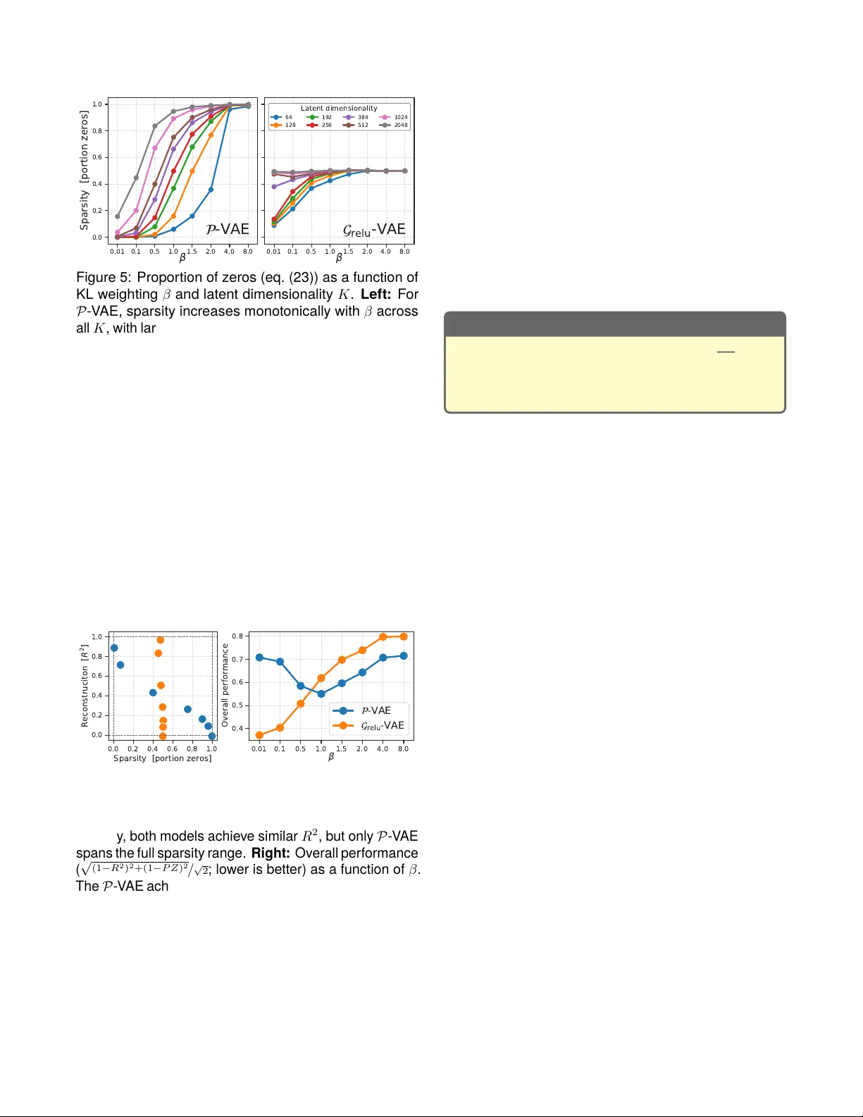
Computation in biological systems is fundamentally energy-constrained, yet standard theories of computation treat energy as freely available. Here, we argue that variational free energy minimization under a Poisson assumption offers a principled path…
Authors: Hadi Vafaii, Jacob L. Yates
Metabolic cost of information processing in P oisson v ariational autoencoders Hadi V afaii, Jacob L. Y ates Redwood Cent er for Theor etical Neuroscience, UC Berk ele y {vafaii,yates}@berkeley.edu Abstract Computation in biological syst ems is fundamentally energy-constr ained, y et standard theories of compu- tation treat energy as freely av ailable. Here, we argue that variational free energy minimization under a P oisson assumption offers a principled path tow ard an energy- aw are theory of computation. Our key observation is that the Kullback-Leibler (KL) divergence term in the Pois- son free energy objectiv e becomes proportional to the prior firing rates of model neurons, yielding an emergent metabolic cost t erm that penalizes high baseline activity . This structure couples an abstract information-theore tic quantity—the coding rat e —to a concret e biophysical variable—the firing rate —which enables a trade-off be- tween coding fidelity and energy expenditure. Such a coupling arises naturally in the Poisson variational autoen- coder ( 𝒫 - V AE)—a brain-inspired generative model that encodes inputs as discret e spik e counts and reco v ers a spiking form of sparse coding as a special case—but is absent from standard Gaussian V AEs. T o demonstrate that this metabolic cost structure is unique to the Poisson formulation, we com pare the 𝒫 - V AE against 𝒢 relu - V AE, a Gaussian V AE with ReL U rectification applied to latent samples, which controls for the non-negativity constraint. Across a syst ematic sweep of the KL term weighting coef- ficient 𝛽 and latent dimensionality , we find that increasing 𝛽 monotonically increases spar sity and reduces av erage spiking activity in the 𝒫 - V AE. In contrast, 𝒢 relu - V AE repr e- sentations remain unchanged, confirming that the effect is specific to Poisson statistics rather than a byproduct of non-negative representations. These results establish Poisson variational infer ence as a promising foundation for a resource-constr ained theory of com putation. Introduction Modern ar tificial intelligence (AI) has achieved im pres- sive breakthroughs with no slowdown in sight. Howe v er , this achiev ement comes at a serious cost : mainstream AI models are energetically inefficient, posing a global sus- tainability thr eat (Hao, 2025). P owering models like Chat- GPT consumes gigaw att-hours, and energy is quickly becoming the unav oidable bottleneck for AI progress (Y ou & Owen, 2025). This is a fundamental physical constraint we cannot engineer our wa y around—there is an urgent need to address this from fir st principles. The energy inefficiency of mainstream AI syst ems orig- inates from a critical design principle: the decoupling of energy and computation (Deacon, 2011; Landauer , 1961). There are no mechanisms internal to architec- tures like transformers that relate computation to energy expenditur e. For a transformer , every tok en is created equal, as far as voltage goes. This is wasteful by design. In sharp contrast, energy-efficiency is a core princi- ple of biological com putation (Olshausen & Field, 1997; Quiroga et al., 2008; Sterling & Laughlin, 2015). Brains run on ∼ 20 watts (Balasubramanian, 2021), yet per form computations that require megaw att-scale data centers to approximat e. This efficiency is likel y driven by the efficient coding hypot hesis (Barlow , 1961, 1972, 1989), which stat es that brains adapt to the statistics of their environments (Simoncelli & Olshausen, 2001), minimiz- ing metabolic cost (Attwell & Laughlin, 2001; Olshausen & Field, 1996; Padamsey & R ochefort, 2023). A com- plementary possibility is that the brain’s representational form—discre te spiking events—de termines the cost struc- ture of the computation itself. Neuromorphic computing aims to bridge biological and ar tificial computation (Mead, 2002), where ev ent-driv en architectur es like Intel’s Loihi (Davies et al., 2018) already “think” in spik es and energy . But we still lack rigorous theoretical foundations to inform future algorithm and hardware co-design. This motivat es the need for an energy-a war e theory of computation that goes beyond the current frameworks, which are limited to time and space complexity (Sipser, 2012; V on Neumann, 1945). Aimone (2025) recently approached this from the hard- ware perspective. He argued that neuromorphic comput- ing has fundamentally different energy scaling compared to the von Neumann architecture. In conventional sys- tems, energy is propor tional to total algorithmic work: ev ery operation incurs a fix ed cost regardless of what is actually being computed. In neuromorphic syst ems, energy is instead propor tional to the cumulative change of state across the computational graph: if a neuron does not spike and its state does not change, no energy is expended. Aimone (2025) fur ther showed that the domi- nant energy terms all scale with the average firing rate, making sparsity the primar y lever for efficiency . Howev er , this analysis addresses only the hardware side. The algorithmic and theoretical foundations remain missing. Here, we demonstrat e how P oisson v ariational infer - ence (V afaii et al., 2024, 2025) naturally leads to the emer - The variational free energy equation: relating model evidence (lef t hand side) to the variational free energy objective ( ELBO = −ℱ ), plus the standard KL objective (used as the star ting point in variational inference). Impor tantly , the left hand side does not depend on the variational parameters, 𝜆 ; theref ore, minimizing ℱ with respect to 𝜆 directly minimizes the original inference KL objective. In shor t : evidence( 𝑥 ; 𝜃 ) = −ℱ ( 𝑥 ; 𝜃 , 𝜆 ) + KL ( 𝑥 ; 𝜃 , 𝜆 ) . log 𝑝 ( 𝑥 ; 𝜃 ) model evidence (log marginal) = E 𝑧 ∼ 𝑞 𝜆 ( 𝑧 | 𝑥 ) log 𝑝 ( 𝑥 | 𝑧 ; 𝜃 ) Reconstruction term ( accuracy ) − 𝒟 KL 𝑞 𝜆 ( 𝑧 | 𝑥 ) 𝑝 ( 𝑧 ; 𝜃 ) KL term ( coding rate ) ELBO( 𝑥 ; 𝜃 , 𝜆 ) = −ℱ ( 𝑥 ; 𝜃 , 𝜆 ) + 𝒟 KL 𝑞 𝜆 ( 𝑧 | 𝑥 ) 𝑝 ( 𝑧 | 𝑥 ; 𝜃 ) KL term ( original objective ) quantifies infer ence quality (1) gence of an energy-aw are objective that learns to trade computational accuracy for energy e xpenditure. We con- trast this with standard Gaussian variational inference (F riston, 2005, 2009, 2010; Kingma & Welling, 2014), re- vealing that such a metabolic cost term is critically absent from the Gaussian formulation. We pro vide a theoretical explanation using information geometry (Amari, 2016): Poisson and Gaussian distributions hav e fundamentally different geometries, and only P oisson realizes the kind of energy-computation coupling that Aimone (2025) ar - gues for . We then conduct comprehensive experiments that confirm these theoretical predictions. Contributions. W e establish from probabilistic first principles that v ariational infer ence under P oisson as- sumptions naturally produces an emergent metabolic term that makes silence cheap , and couples information rat e to firing rat e . This cost structure is strikingly similar to what Aimone (2025) arrives at from hardwar e principles: that energy-efficient neuromorphic computation requires algorithms where energy scales with change-of-state rather than total work, and that spar sity (silence) should be free. The conv ergence of these two independent lines of reasoning—hardware and information theory— positions Poisson variational infer ence as a promising foundation for resource-constrained theories of com puta- tion that treat energy expenditur e as a core consideration. Background Notation. We denote scalars 𝑠 ∈ R with lowercase lett ers, vectors 𝑣 ∈ R 𝑑 with bold lowercase, and matrices M ∈ R 𝑚 × 𝑛 with bold uppercase. W e use red / blue color - coding to indicate the inference (encoder) / generative (decoder) components of each model, respectivel y . Perception as inference. Brains nev er hav e access to ground truth information; therefor e, brains must alwa ys infer the state of the world from par tial and of ten noisy obser vations. This can be modeled using Bay es’ rule: 𝑝 brain ( 𝑧 | 𝑥 ; 𝜃 ) posterior = 𝑝 brain ( 𝑥 | 𝑧 ; 𝜃 ) 𝑝 brain ( 𝑧 ; 𝜃 ) 𝑝 brain ( 𝑥 ; 𝜃 ) , (2) where 𝑥 ∈ R 𝑀 are obser ved data (e.g., images), and 𝑧 are 𝐾 -dimensional latent variables internal to the agent. All distributions 𝑝 brain ( · ; 𝜃 ) represent subjective beliefs internal to the agent, hence the subscript brain ; and 𝜃 are adaptable paramet ers of these internal models (e.g., synaptic weights in brains, or neural net parameters). T o simplify notation, we drop the brain subscript. But it should be clear from the conte xt (and the blue 𝜃 ) that we are working with distributions internal to the agent. V ariational inference and the free energy objective. The optimal Ba y esian pos terior (eq. (2)) is often in- tractable due to the marginal distribution appearing in the denominator , motivating the need for appro ximations. V ariational inference (VI; Blei e t al. (2017)) offers a powerful framework for approximat e inference. In VI, we introduce a distribution 𝑞 𝜆 ( 𝑥 ) , termed the appro ximat e post erior , with variational paramet ers 𝜆 that are optimized to minimize the Kullback -Leibler (KL) divergence: 𝜆 * = argmin 𝜆 𝒟 KL 𝑞 𝜆 ( 𝑧 | 𝑥 ) 𝑝 ( 𝑧 | 𝑥 ; 𝜃 ) . (3) Howe v er , directly optimizing the KL objective (eq. (3)) requires access to the intractable posterior (eq. (2)). V ari- ational infer ence circumvents this by instead optimizing an equivalent objective, the E vidence L ow er BO und , or v ariational free energy ( ELBO = −ℱ ; eq. (1)), which can be constructed and ev aluated using only the approx- imate posterior , the prior , and the likelihood. Maximizing ELBO (or equivalently , minimizing ℱ ) directly minimizes the original KL objectiv e (eq. (3)). See appendix for a pedagogical derivation of eq. (1) using simple algebra. Distinguishing the two KL terms in the free energy . Note how a second KL term appears in the ELBO / ℱ expansion of eq. (1). This KL com ponent of ℱ is dif- ferent from the original one in eq. (3) (which was our starting point), and can be interpreted as the informa- tion coding rate : the additional bits required to encode stimulus-specific information in the posterior beyond what is already captured by the prior (Alemi et al., 2018; Hob- son, 1969; Thomas M. Cov er, 2006). Hereafter , “KL term” refers ex clusively to the coding- rate KL within the ℱ definition: 𝒟 KL ( p osterior ‖ prior ) . Three distributions, one ℱ . T o fully specify ℱ (eq. (1)), we need to choose three distributions: the approximate posterior 𝑞 𝜆 ( 𝑧 | 𝑥 ) , the prior 𝑝 ( 𝑧 ; 𝜃 ) and the conditional likelihood 𝑝 ( 𝑥 | 𝑧 ; 𝜃 ) . In both machine learning and theo- retical neuroscience, people of ten choose Gaussians for all three. Howev er , this choice is typically motivat ed by conv ention and com putational tractability . The latent representational form. The choice of prior and the approximat e posterior is par ticularly impor tant, because it determines the represent ational for m of the latent space, significantly impacting model behavior and properties. Below , we will demonstrate that choosing Poisson instead of Gaussian leads to intriguing mathe- matical properties in the free energy objective. Poisson variational autoencoder ( 𝒫 -V AE). Brains use discret e spike counts to represent and communicate information. Mo tivat ed by this biological reality , (V afaii et al., 2024) introduced the 𝒫 - V AE, which replaces the Gaussian latents in a standard Gaussian V AE ( 𝒢 - V AE; Kingma and W elling (2014)) with Poisson. V ariational parameters in V AEs. In a 𝒫 - V AE, the vari- ational parame ter 𝜆 ∈ R 𝐾 ⩾ 0 is a 𝐾 -dimensional v ector of firing rates, one per model neuron. In a 𝒢 - V AE, to fully specify a (factorized) Gaussian approximat e poste- rior we need both a mean vector 𝜇 ∈ R 𝐾 , and variance 𝜎 2 ∈ R 𝐾 ⩾ 0 . In other words, for a 𝒢 -V AE: 𝜆 ≡ ( 𝜇 , 𝜎 2 ) . Inference with learned encoder neur al networks. In both 𝒫 - V AE and 𝒢 - V AE, an encoder neural network maps input data to the corr esponding distributional parame- ters required for constructing the appro ximate posterior 𝑞 𝜆 ( 𝑧 | 𝑥 ) . In other words: 𝜆 ( 𝑥 ) = enc ( 𝑥 ; 𝜑 ) , where 𝜑 are paramet ers of the encoder network. In V AEs, 𝜃 and 𝜑 — paramet ers of the decoder and encoder networks—are jointly optimized by minimizing ℱ ( 𝑥 ; 𝜃 , 𝜑 ) (eq. (1)). Residual parameterization in the 𝒫 -V AE. The 𝒫 - V AE adopts a residual parameterization: instead of producing the full post erior rat es 𝜆 ( 𝑥 ) , the encoder network outputs a r esidual gain modulation, 𝛿 𝜆 ( 𝑥 ) = enc ( 𝑥 ; 𝜑 ) ∈ R 𝐾 ⩾ 0 , that is element-wise multiplied to learnable prior firing rates 𝜆 0 ∈ R 𝐾 ⩾ 0 , yielding the final posterior rates: 𝜆 ( 𝑥 ) = 𝜆 0 ⊙ 𝛿 𝜆 ( 𝑥 ) . (4) And the 𝒢 - V AE residual paramet erization is defined as: 𝜇 ( 𝑥 ) = 𝜇 0 + 𝛿 𝜇 ( 𝑥 ) , 𝜎 ( 𝑥 ) = 𝜎 0 ⊙ 𝛿 𝜎 ( 𝑥 ) . (5) This residual parameterization is motiv ated by both computational and biological considerations: maintaining a base firing rate and com puting only stimulus-specific residuals is more efficient and is reminiscent of predictiv e coding (Rao & Ballard, 1999), while the multiplicative in- teraction functionally implements gain control (Schwartz & Simoncelli, 2001), similar to the modulation obser ved in top-down cor tical interactions (Gilber t & Li, 2013). In this residual paramet erization, the 𝒫 - V AE approxi- mate posterior and prior are given by: 𝑞 𝜆 ( 𝑧 | 𝑥 ) = 𝒫 ois( 𝑧 ; 𝜆 0 ⊙ 𝛿 𝜆 ( 𝑥 )) , (6) 𝑝 ( 𝑧 ; 𝜃 ) = 𝒫 ois( 𝑧 ; 𝜆 0 ) , (7) where 𝒫 ois is the Poisson probability density function: 𝒫 ois( 𝑧 ; 𝜆 ) = 𝜆 𝑧 𝑒 − 𝜆 𝑧 ! . A metabolic cost term emerg es in the 𝒫 - V AE, but not in 𝒢 - V AE With this background, we are now ready to introduce the main intriguing property of the 𝒫 - V AE free energy (eq. (1)): the KL term ( coding rate ; Alemi et al. (2018)) becomes linearly proportional to the prior firing rates 𝜆 0 , encouraging the model to maintain a low baseline firing. In the appendix, we derive the KL term for both 𝒫 - V AE and 𝒢 - V AE. Assuming a single latent dimension ( 𝐾 = 1 ), the final expressions are given by: Poisson : 𝒟 KL = 𝜆 0 𝑓 ( 𝛿𝜆 ) , (8) Gaussian : 𝒟 KL = 1 2 𝛿 𝜇 2 𝜎 2 0 + 𝑔 ( 𝛿 𝜎 2 ) , (9) where 𝑓 ( 𝑦 ) : = 𝑦 log 𝑦 − 𝑦 + 1 and 𝑔 ( 𝑦 ) : = 𝑦 − 1 − log 𝑦 . Quadratic approximation. In the appendix, we com- pute the leading-order T aylor expansions of the nonlin- earities 𝑓 ( · ) and 𝑔 ( · ) , re vealing a parallel structure: Poisson : 𝑓 ( 𝛿 𝜆 ) ≈ 1 2 (log 𝛿 𝜆 ) 2 , (10) Gaussian : 𝑔 ( 𝛿 𝜎 2 ) ≈ 1 2 (log 𝛿 𝜎 2 ) 2 . (11) Figure 1 visualizes 𝑓 and 𝑔 , and their quadratic appro xi- mations. Notably , 𝑓 grows superquadratically for positive deviations, imposing a stronger penalty on firing rate increases than decreases. Equations (8) to (11) yield the approximat e KL terms: Poisson : 𝒟 KL ≈ 1 2 𝜆 0 (log 𝛿 𝜆 ) 2 , (12) Gaussian : 𝒟 KL ≈ 1 2 𝛿 𝜇 2 𝜎 2 0 + (log 𝛿 𝜎 ) 2 . (13) KL div ergence: Poisson v ersus Gaussian Despite the local similarity (eqs. (10) and (11)), the ap- pro ximate KL terms (eqs. (12) and (13)) reveal two fun- damental structural differences. Figure 1: Per -dimension cost contributions of the KL term for the 𝒫 - V AE (left) and 𝒢 - V AE (right), plotted as a function of the log-residual parameters 𝛿 𝑢 = log 𝛿 𝜆 and 𝛿 𝑣 = log 𝛿 𝜎 2 , respectiv ely . Solid cur ves show the ex act nonlinearities 𝑓 (eq. (8)) and 𝑔 (eq. (9)); dashed cur ves show their quadratic approximations. Both func- tions share a minimum of zero at the identity residual ( 𝛿 𝑢 = 𝛿 𝑣 = 0 , i.e., post erior = prior) and are locally quadratic, but 𝑓 grows superquadratically for positive deviations, imposing a stronger penalty on firing rate in- creases than decreases. The first difference concerns scaling . For the Pois- son, the KL is propor tional to the prior rat e 𝜆 0 ; for the Gaussian, the mean-shif t cost is scaled by the precision 1 / 𝜎 2 0 , which is independent of the prior mean. This has a direct consequence for what each model consider s “cheap”: the Poisson objective can reduce coding costs by lowering the absolute firing rate ( 𝜆 0 → 0 ), i.e., “silence is cheap”; while the Gaussian can reduce costs by in- flating the prior variance ( 𝜎 2 0 → ∞ ), i.e., “ignorance is cheap”. Additionally , the Poisson scaling (eq. (8)) is rem- iniscent of the L1 penalty in sparse coding (Olshausen & Field, 1996), but with an adaptivel y modulated penalty strength 𝑓 ( 𝛿 𝜆 ) rather than a fixed coefficient. The second difference concerns translation invari- ance . The Gaussian mean-shif t term depends only on the difference 𝛿 𝜇 2 = ( 𝜇 − 𝜇 0 ) 2 , so the cost is identical whether 𝜇 0 is 0 or 1000. In other words, the Gaussian framew ork has no metabolic floor and is indifferent to the absolute magnitude of activity . In contrast, the Poisson KL breaks this inv ariance: its linear dependence on 𝜆 0 grounds the computation in a regime where zero activity is the uniq ue lowest-cos t state. The differences arise from information g eometry . Both differences are conseq uences of information geom- etry (Amari, 2016). The KL divergence is locally quadratic in the natural (canonical) parameters of the exponential family . F or the Poisson, the natural parameter is log 𝜆 , and the Fisher information metric in this natural space is 𝐼 = 𝜆 . This yields a cur vature scaled by the rate itself: 𝜆 0 ( log 𝛿 𝜆 ) 2 . For the Gaussian mean variable 𝜇 , the nat- ural paramet er is scaled by variance, but the metric is determined by precision ( 𝐼 = 1 /𝜎 2 ), which is, crucially , independent of the mean. This specific coupling betw een the metric and the paramet er magnitude in the Poisson distribution is what gives rise to the emergent metabolic cost (but is absent in the location-scale Gaussian family). Summary so far . Unlike the Gaussian case, the Pois- son KL admits a metabolic cost interpretation, owing to its linear dependence on the prior rate: 𝒟 KL ≈ 𝜆 0 (log 𝛿 𝜆 ) 2 : Poisson KL: a metabolic cost term interpretation T o encode information efficiently , maintain low baseline firing rates whenev er possible. The P oisson KL divergence term couples firing rate to information rate The previous section established that the Poisson KL is propor tional to the prior firing rate 𝜆 0 . We now argue that this mathematical structure carries a deeper significance, by ex amining what the KL term itself measures. Is KL “just ” a regularizer? In much of the machine learning literature, the KL term in the ELBO is treated as a regularizer: a penalty that prev ents the appro ximate posterior from stra ying too far from the prior , analogous to weight decay or an L2 penalty . Under this view , the KL is just another knob to tune. This framing, while operationally useful, obscures the profound meaning of the KL term. T o address this, we ask: What, precisely , does the KL term quantify in the conte xt of inference? KL as a measur e of information gain. Hobson (1969) addressed this question from first principles. He was in- ter ested in deriving a uniq ue functional that measures the information gained when updating from a prior belief 𝑃 to a posterior belief 𝑄 . Starting from a small set of “intuitively reasonable proper ties”—reparamet erization inv ariance, additivity for independent sources, monotonicity , and a composition rule—he pro ved that the KL divergence is the only e xpression that quantifies information gain while satisfying those intuitive requirements. In sum: KL as a unique measure of information gain 𝒟 KL ( 𝑄 ‖ 𝑃 ) is the unique expr ession for the information contained in a message which alters the probabilities from 𝑃 to 𝑄 (Hobson, 1969). Abstract, information theoretic per spective: KL as information r ate. This result reframes the KL term from just a regularizer into something far more fundamental: it is the infor mation rat e —the number of bits per inference step that the stimulus-driven posterior contains bey ond what was already present in the prior . F urther , KL is not one of many possible measures, or just a definition: it is “ the ” measure, uniquely determined by basic desiderata. Concrete, biophysical perspective: 𝜆 0 as metabolic rate. Now consider what appear s on the right hand side in the P oisson KL expr ession (eq. (8)). The prior rate 𝜆 0 is not an abstract parameter . It repr esents a concre te biophy sical q uantity: the baseline number of spikes per unit time. In a pot ential neuromorphic implementation, it has energy units. As a model of spiking in the brain, it costs A TP (or at least, the synapses responding to those spikes cost A TP (Attwell & Laughlin, 2001)). Thus, the prior rate 𝜆 0 is—in this literal sense—a metabolic rat e . Merging the two perspectives: The P oisson KL term is a joint cost over information and energy , that couples an abstract “Information Rat e” (bits / inference step) to a concret e “Metabolic Rate” (spikes / inference step): Poisson KL: Information Rate ↔ Metabolic Rate 𝒟 KL 𝒫 ois( 𝑧 ; 𝜆 0 ⊙ 𝛿 𝜆 ( 𝑥 )) 𝒫 ois( 𝑧 ; 𝜆 0 ) = 𝜆 ⊤ 0 𝑓 ( 𝛿 𝜆 ) Impor tantly , the variational fr ee energy objec- tive (eq. (1)) was derived from purely probabilistic considerations—nowhere did we impose an explicit energy constraint. Y et, a metabolic cost term emerged from the mathematics of v ariational inference under Poisson (but not Gaussian) assum ptions. Interim conclusion (theor y). We hav e theoreticall y es- tablished that the P oisson KL t erm couples metabolic rat e to information rate—a feature with no analog in the Gaus- sian framework. We explained this difference through the lens of information geometr y , and traced it back to the mean-variance coupling in Poisson. Bey ond mean-variance coupling, another fundamental difference between Poisson and Gaussian distributions is their suppor t: P oisson is nonnegative, whereas Gaus- sian is unconstrained. Could restricting the Gaussian to positive values induce a similar metabolic cost structure? The Gaussian-Rectified 𝒢 relu - V AE T o control for the positive-support constraint, we apply a ReL U activation to Gaussian samples before passing them to the decoder . The ReL U choice is motivat ed by sev eral converging lines of evidence: Whittington et al. (2023) showed that applying ReL U to 𝒢 - V AE, combined with activity penalties, produces disentangled represen- tations that can outperform 𝛽 - V AEs (Higgins et al., 2017); and Bric ken et al. (2023) showed that combining ReL U with noisy in puts appro ximates sparse coding. The rectification step modifies the decoding pathway . Given a decoder neural network dec ( · ; 𝜃 ) with paramet ers 𝜃 , the reconstruction is defined as ˆ 𝑥 = dec ( ℎ ; 𝜃 ) , where ℎ ≡ ℎ ( 𝑧 ) is a function of the latent samples 𝑧 : Poisson : ℎ = 𝑧 , (14) Gaussian : ℎ = relu( 𝑧 ) = max( 0 , 𝑧 ) . (15) W e ref er to this resulting rectified Gaussian model as 𝒢 relu - V AE. Figure 2 compares the appro ximate posterior distributions of 𝒫 - V AE and 𝒢 relu - V AE. Figure 2: Appro ximat e posterior distributions for a single latent dimension. Lef t: The 𝒫 - V AE post erior is a P oisson distribution over nonnegative integers (rate = 2 ). Right: The (unnormalized) 𝒢 relu - V AE posterior (solid orange) is obtained b y applying a ReL U to Gaussian samples (dashed gra y , 𝜇 = 0 , 𝜎 = 1 ). Both models produce non- negative latent representations, but through fundamen- tally different mechanisms: discret e counting statistics versus continuous rectification. Linear decoders, closed-form reconstruction loss, and the variance penalty Recall from eq. (1) that the free energy objective decom- poses into two terms: ℱ = ℒ recon + 𝒟 KL . So far , we hav e focused solely on the KL term ( 𝒟 KL ), and derived its closed-form expression for both Poisson and Gaussian latent variables (eqs. (8) and (9)). We now turn t o the reconstruction term. The reconstruction term. ℒ recon measures the q uality of the latent representation: if the encoding is high fidelity , the data sample 𝑥 will hav e high expected likelihood un- der the appro ximate posterior . Throughout this work, we assume a Gaussian conditional likelihood with 2 𝜎 2 dec = 1 , yielding the mean sq uared error reconstruction loss: ℒ recon = E 𝑧 ∼ 𝑞 𝜆 ( 𝑧 | 𝑥 ) − log 𝑝 ( 𝑥 | 𝑧 ; 𝜃 ) = E 𝑧 ∼ 𝑞 𝜆 ( 𝑧 | 𝑥 ) ‖ 𝑥 − dec( 𝑧 ; 𝜃 ) ‖ 2 2 , (16) where dec( 𝑧 ; 𝜃 ) is the decoder neural network. Linear decoders and closed-form reconstruction. Consider a linear decoder dec ( 𝑧 ; 𝜃 ) = Φ 𝑧 , where Φ ≡ 𝜃 are the decoder parameters. This is a standard choice in theoretical neuroscience (Olshausen & Field, 1996; Rao & Ballard, 1999), where Φ is often called the dictionary . In machine learning, Lucas et al. (2019) relied on linear V AEs to study posterior collapse, and Shao et al. (2025) used them to introduce zero-v ariance gradients for V AEs. Given a linear decoder , the expectation in eq. (16) de- pends only on the first and second moments of 𝑞 , allowing for an analytical derivation (see appendix): ℒ recon = ‖ 𝑥 − Φ E 𝑞 [ 𝑧 ] ‖ 2 2 mean penalty + diag ( Φ ⊤ Φ ) ⊤ V ar 𝑞 [ 𝑧 ] variance penalty . (17) The variance penalty . The second term in eq. (17) pe- nalizes high posterior uncer tainty . For Poisson, V ar 𝑞 [ 𝑧 ] = 𝜆 , linking v ariance directly to firing rate. This intro- duces a sparsity pressure distinct from the KL mecha- nism (eq. (12)): dimensions with larger dictionar y norms ( [ Φ ⊤ Φ ] 𝑖𝑖 ) must maintain lower firing rates ( 𝜆 𝑖 ) to mini- mize free energy . Biologically , this say s that neurons with larger receptive fields should fire more sparingly . For the standard Gaussian, variance is independent of the mean, so no such spar sity interpretation arises. But what about the rectified 𝒢 relu - V AE? For 𝒢 relu - V AE, we need the moments of ℎ = relu ( 𝑧 ) . W e carry out these calculations in the appendix and present the final results here: 𝑚 : = E 𝑞 [ ℎ ] = 𝜇 ⊙ Φ( 𝜁 ) + 𝜎 ⊙ 𝜑 ( 𝜁 ) , (18) 𝑣 : = V ar 𝑞 [ ℎ ] = ( 𝜇 2 + 𝜎 2 ) ⊙ Φ( 𝜁 ) + ( 𝜇 ⊙ 𝜎 ) ⊙ 𝜑 ( 𝜁 ) − 𝑚 2 , (19) where 𝜁 : = 𝜇 ⊘ 𝜎 is the standardized mean, and Φ( · ) and 𝜑 ( · ) are the standard normal CDF and PDF , respectivel y . Figure 3 visualizes these moments. Rectification promotes spar sity . The mean-variance coupling in the 𝒢 relu - V AE (eqs. (18) and (19)) enables suppressing the variance by pushing the posterior mean 𝜇 → −∞ , silencing a latent dimension entirely . This pro vides the 𝒢 relu - V AE with a spar sity mechanism through the reconstruction term. Conclusion (theor y). Both 𝒫 - V AE and 𝒢 relu - V AE e x- hibit variance-driv en sparsity pressures through the re- construction term, but only the Poisson KL directly pe- nalizes metabolic cost. Does this mathematical structure drive energy efficiency in practice? In the next section, we formulate specific predictions from our theor y and test them experimentally . Figure 3: Mean (lef t) and v ariance (right) of relu ( 𝑧 ) for 𝑧 ∼ 𝒩 ( 𝜇 , 𝜎 2 ) , plotted as a function of 𝜇 for sev eral v alues of 𝜎 . The mean (eq. (18)) behav es similar to sof tplus (dashed), approaching the identity for 𝜇 ≫ 0 and vanishing for 𝜇 ≪ 0 . The v ariance (eq. (19)) behaves as a sigmoid-like (but steeper) gating function, saturating at 𝜎 2 for 𝜇 ≫ 0 and vanishing for 𝜇 ≪ 0 . Crucially , rectification couples mean and variance: pushing 𝜇 → −∞ suppresses both simultaneously , providing a mechanism for the 𝒢 relu - V AE to achieve sparse, low-variance representations. Empirical validation: the Poisson KL term promo tes sparsity Experimental design: the 𝛽 coefficient. T o test the metabolic cost interpretation, we introduce a weighting paramet er 𝛽 that controls the relative strength of the KL term in the free energy (eq. (1)): ℱ = ℒ recon + 𝛽 𝒟 KL , (20) which is identical to the 𝛽 - V AE framework (Higgins et al., 2017). By varying 𝛽 , we modulate the pressure from the KL term and obser ve how each model responds. Hypothesis. Since only the Poisson KL acts as a metabolic cost term (eq. (12) vs. eq. (13)), we hypo the- size that increasing 𝛽 will systematically increase spar - sity in 𝒫 - V AE representations, while having little effect on 𝒢 relu - V AE representations. The full analytical free energy . Assuming a linear decoder , the complete objective is: ℱ = ‖ 𝑥 − Φ 𝑚 ‖ 2 2 + diag( Φ ⊤ Φ ) ⊤ 𝑣 + 𝛽 𝒟 KL (21) where 𝑚 = 𝑣 = 𝜆 for 𝒫 - V AE, and 𝑚 , 𝑣 are given b y eqs. (18) and (19) for 𝒢 relu - V AE. Comprehensive model com parison. In this paper , we work with 𝒫 - V AE and 𝒢 relu - V AE architectures. T able 1 pro vides a comprehensive summary of model proper ties. T able 1: Poisson V AE ( 𝒫 -V AE) and Gaussian-Rectified V AE ( 𝒢 relu -V AE) architectures . The linear decoder reconstructs ˆ 𝑥 = Φ ℎ , where ℎ is the (possibly rectified) lat ent representation. Within this setup, the closed- form reconstruction loss is giv en by : ℒ recon = 1 / 2 ‖ 𝑥 − Φ 𝑚 ‖ 2 2 + diag( Φ ⊤ Φ ) ⊤ 𝑣 , where 𝑚 and 𝑣 are the mean and v ariance of ℎ under the approximat e post erior 𝑞 𝜆 ( 𝑧 | 𝑥 ) . This results in a closed-form free energy objective, ℱ = ℒ recon + 𝛽 𝒟 KL . For the Poisson model, 𝜆 0 denotes the learnable prior rates and 𝛿 𝜆 = 𝜆 ⊘ 𝜆 0 is the element- wise multiplicative residual, interpreted as gain modulation. For the Gaussian model, 𝜇 0 , 𝜎 0 denote the prior mean and scale, with additive residual 𝛿 𝜇 = 𝜇 − 𝜇 0 and multiplicative residual 𝛿 𝜎 = 𝜎 ⊘ 𝜎 0 . For the Gaussian moments, we have defined 𝜁 : = 𝜇 ⊘ 𝜎 , and 𝜑 ( · ) and Φ( · ) are the standard normal PDF and CDF , respectiv ely . Model Approx. posterior 𝑞 𝜆 ( 𝑧 | 𝑥 ) (for a single latent variable) Decoder ˆ 𝑥 = Φ ℎ Moments of ℎ under 𝑞 𝜆 ( 𝑧 | 𝑥 ) : 𝑚 = E 𝑞 [ ℎ ] , 𝑣 = E 𝑞 [ ℎ 2 ] − 𝑚 2 KL divergence , 𝒟 KL (coding rate) 𝒫 - V AE 𝑞 𝜆 ( 𝑧 | 𝑥 ) = 𝜆 𝑧 𝑒 − 𝜆 𝑧 ! 𝑧 ∈ Z ⩾ 0 , 𝜆 ( 𝑥 ) ∈ R ⩾ 0 ℎ = 𝑧 𝑚 = 𝜆 𝑣 = 𝜆 𝒟 KL = 𝜆 ⊤ 0 𝑓 ( 𝛿 𝜆 ) 𝑓 ( 𝑦 ) = 𝑦 log 𝑦 − 𝑦 + 1 𝒢 relu - V AE 𝑞 𝜇 , 𝜎 2 ( 𝑧 | 𝑥 ) = 1 √ 2 𝜋 𝜎 2 exp − ( 𝑧 − 𝜇 ) 2 2 𝜎 2 𝑧 ∈ R , 𝜇 ( 𝑥 ) ∈ R , 𝜎 2 ( 𝑥 ) ∈ R ⩾ 0 ℎ = relu( 𝑧 ) 𝑚 = 𝜇 ⊙ Φ( 𝜁 ) + 𝜎 ⊙ 𝜑 ( 𝜁 ) 𝑣 = ( 𝜇 2 + 𝜎 2 ) ⊙ Φ( 𝜁 ) + 𝜇 ⊙ 𝜎 ⊙ 𝜑 ( 𝜁 ) − 𝑚 2 𝒟 KL = 1 2 1 ⊤ 𝛿 𝜇 2 𝜎 2 0 + 𝑔 ( 𝛿 𝜎 2 ) 𝑔 ( 𝑦 ) = 𝑦 − 1 − log 𝑦 Methods. Following V afaii et al. (2024), we trained 𝒫 - V AE and 𝒢 relu - V AE models on whitened 16 × 16 natural im- age patches from the van Hateren dataset (van Hateren & van der Schaaf, 1998). For each model family , we trained multiple instances across a grid of latent dimensionalities 𝐾 and KL weighting coefficients 𝛽 (eq. (20)): 𝐾 ∈ { 64 , 128 , 192 , 256 , 384 , 512 , 1024 , 2048 } , 𝛽 ∈ { 0 . 01 , 0 . 1 , 0 . 5 , 1 . 0 , 1 . 5 , 2 . 0 , 4 . 0 , 8 . 0 } . Architectures. Both model families used identical architectur es—a linear encoder and decoder with Gaus- sian likelihood (eqs. (16) and (17))—differing only in their distributional assum ptions ov er the latents. Representations. Af ter training, we extract represen- tations by passing validation data samples 𝑥 through the encoder to obtain the posterior 𝑞 𝜆 ( 𝑧 | 𝑥 ) , from which we sample latent representations 𝑧 . We then use 𝑧 to ev aluate sparsity and metabolic cost. Metrics. We quantify energy efficiency using two com- plementary metrics, aver aged ov er the validation set : (Metabolic Cost) 𝑀 𝐶 : = mean activity of 𝑧 (22) (Sparsity) 𝑃 𝑍 : = propor tion of zeros in 𝑧 (23) Result #1: Only 𝒫 -V AE KL works as a metabolic cost. Figure 4 show s the mean neural activity as a function of 𝛽 . For 𝒫 - V AE, increasing 𝛽 reduces metabolic cost by nearly two order s of magnitude, confirming that the Poisson KL acts as an effective metabolic cost term whose strength is directly controlled by 𝛽 . For 𝒢 relu - V AE, mean activity remains flat across all 𝛽 values, confirming the theore tical prediction that the Gaussian KL is decoupled from the magnitude of neural activity . 0.01 0.1 0.5 1.0 1.5 2.0 4.0 8.0 1 0 2 1 0 1 1 0 0 1 0 1 1 0 2 P osterior samples mean - V A E 0.01 0.1 0.5 1.0 1.5 2.0 4.0 8.0 r e l u - V A E Latent dimensionality 64 128 192 256 384 512 1024 2048 Figure 4: Metabolic cost (eq. (22)) as a function of KL weighting 𝛽 for different latent dimensionalities. Lef t : 𝒫 - V AE shows dramatic reduction in metabolic cost with increasing 𝛽 , spanning nearly two orders of magnitude. Right : 𝒢 relu - V AE shows no systematic change, remaining near baseline across all 𝛽 values. This confirms that the metabolic cost structure is unique to Poisson. Result #2: Only 𝒫 -V AE KL promotes sparsity . Fig- ure 5 shows sparsity as a function of 𝛽 . F or 𝒫 - V AE, the proportion of silent neurons increases monotonically with 𝛽 across all latent dimensionalities, reaching near - complete sparsity at high 𝛽 . For 𝒢 relu - V AE, sparsity saturat es at appro ximately 50% —the e xpected propor tion of negative samples under a symmetric Gaussian—and is insensitive to 𝛽 bey ond this floor . This 50% ceiling is consistent with the ReL U mechanism: rectification (and the variance penalty) si- lences roughly half the neurons by construction, but the Gaussian KL pro vides no additional pressure to increase sparsity bey ond this point. 0.01 0.1 0.5 1.0 1.5 2.0 4.0 8.0 0.0 0.2 0.4 0.6 0.8 1.0 Sparsity [portion zer os] - V A E 0.01 0.1 0.5 1.0 1.5 2.0 4.0 8.0 r e l u - V A E Latent dimensionality 64 128 192 256 384 512 1024 2048 Figure 5: Propor tion of zeros (eq. (23)) as a function of KL weighting 𝛽 and latent dimensionality 𝐾 . Lef t: For 𝒫 - V AE, sparsity increases monotonicall y with 𝛽 across all 𝐾 , with larger 𝐾 achieving higher spar sity at the same 𝛽 . Right: For 𝒢 relu - V AE, sparsity plateaus at 50% for all 𝛽 ⩾ 1 . 0 , regardless of 𝐾 . See Fig. 7 for a pie char t visualization of the 𝐾 = 512 results. Result #3: 𝒫 -V AE and 𝒢 relu -V AE achieve compara- ble reconstruction accuracy at matched sparsity , but only Poisson enables a trade-off. Figure 6 (lef t) shows that at matched lev els of spar sity , bo th models achiev e comparable reconstruction quality . Therefore, the 𝒫 - V AE does not sacrifice accuracy to become sparse. The k e y differ ence is controllability: 𝒫 - V AE admits a smooth trade-off betw een spar sity and reconstruction, tunable via 𝛽 (Fig. 6, right). In contrast, 𝒢 relu - V AE spar- sity is locked near 50% regardless of 𝛽 , and increasing 𝛽 worsens reconstruction without affecting sparsity . 0.0 0.2 0.4 0.6 0.8 1.0 Sparsity [portion zer os] 0.0 0.2 0.4 0.6 0.8 1.0 R e c o n s t r u c i t o n [ R 2 ] 0.01 0.1 0.5 1.0 1.5 2.0 4.0 8.0 0.4 0.5 0.6 0.7 0.8 Overall perfor mance - V A E r e l u - V A E Figure 6: Reconstruction–sparsity trade-off for 𝐾 = 512 . Left: Reconstruction quality ( 𝑅 2 ∈ [ −∞ , 1] ) versus spar- sity ( 𝑃 𝑍 ∈ [0 , 1] ; eq. (23)) across all 𝛽 values. At matched sparsity , both models achiev e similar 𝑅 2 , but only 𝒫 - V AE spans the full spar sity range. Right: Overall per formance ( √ (1 − 𝑅 2 ) 2 +(1 − 𝑃 𝑍 ) 2 / √ 2 ; lower is better) as a function of 𝛽 . The 𝒫 - V AE achieves its optimum at 𝛽 = 1 , corresponding to the standard ELBO (eq. (1)), and exhibits a U-shaped cur ve reflecting a genuine trade-off between reconstruc- tion and sparsity . In contrast, the 𝒢 relu - V AE ov erall perfor - mance degrades monotonically as 𝛽 increases, reflecting that stronger KL weighting hur ts reconstruction without yielding additional sparsity gains. Conclusions and Discussion W e showed that variational inference under Poisson as- sumptions yields a KL term with a metabolic cost inter - pretation, enabling a principled trade-off between com- putational accuracy and energetic cost. This structure is absent in Gaussian formulations—ev en when rectified— a result we explained using information geometry and verified em pirically . Combined with the rate-distortion perspective developed below , these results position Pois- son variational inference as a promising foundation for energy-a war e theories of computation that could inform algorithm and hardware co-design for efficient AI. Main takea wa ys • Gaussian ( ignorance is cheap ): 𝒟 KL ∝ 𝛿 𝜇 2 𝜎 2 0 + . . . • Poisson ( silence is cheap ): 𝒟 KL ∝ 𝜆 0 (log 𝛿 𝜆 ) 2 • Poisson 𝒟 KL : Metabolic Rate ↔ Information Rat e Connection to r ate-distortion theor y . We developed our theory within variational inference (Blei et al., 2017), but an equivalent formulation arises from rate-dis tortion theory (RD T ; Alemi et al. (2018) and Thomas M. Cover (2006)). In RD T , we minimize a task loss ℒ task subject to a finite information rate budget ℬ , yielding the objective: minimize : ℒ = ℒ task + 𝛽 𝒟 KL ( s.t. 𝒟 KL ⩽ ℬ ) . (24) where 𝛽 is a Lagrange multiplier . Equation (24) is mathematically identical to the 𝛽 - weighted free energy ( ℱ = ℒ recon + 𝛽 𝒟 KL ; eq. (20)), but with a general task loss in place of reconstruction. Our main contribution is a metabolic cost interpre tation of 𝒟 KL ( ℬ ↔ energy budget ), ex clusively under Poisson latent variables. This opens two directions for future work. Bey ond perception. Since eq. (24) holds for any task loss ℒ task , the metabolic-information coupling e xt ends bey ond autoencoding in visual perception to any setting where a task can be formulated as a well-defined loss function—including behavior , cognition, and bey ond. Bey ond Poisson. Cor tical neurons of ten exhibit super - Poisson variability , well captured by negative binomial distributions (Goris et al., 2014). The negative binomial KL diver gence is also proportional to prior firing rates (Zhang et al., 2025), additionally modulated by a shape paramet er . This suggests that our metabolic cost result generalizes broadly to count-based distributions. Con- tinuous positive-support distributions such as gamma or in v erse Gaussian offer another axis of comparison, controlling for positivity without discret eness. Empirical tests of these generalizations are lef t for future work. References Aimone, J. B. (2025). Neuromorphic computing: A theo- retical framew ork for time, space, and energy scaling. Alemi, A., Poole, B., Fischer , I., Dillon, J., Saurous, R. A., & Murphy , K. (2018, July). Fixing a broken ELBO. In J. Dy & A. Krause (Eds.), Proceedings of the 35th inter - national confer ence on machine learning (pp. 159– 168, V ol. 80). PMLR. https:// proceedings.mlr .press/ v80/ alemi18a.html Alhazen. (1011–1021 AD). Book of optics (kitab al-manazir) . https : / / archiv e . org / details / TheOpticsOfIbnAlHa ythamBooksI Amari, S. - i. (2016). Infor mation geometry and its appli- cations (V ol. 194). Springer. https:// doi.org/ 10.1007/ 978- 4- 431- 55978- 8 . Attwell, D., & Laughlin, S. B. (2001). An energy budget for signaling in the grey matter of the brain. Journal of Cerebral Blood Flow & Metabolism , 21 (10), 1133– 1145. https:// doi.org/ 10.1097/ 00004647- 200110000- 00001 . Balasubramanian, V . (2021). Brain power. Proceed- ings of the National Academ y of Sciences , 118 (32), e2107022118. https : / / doi . org / 10 . 1073 / pnas . 2107022118 . Barlow, H. B. (1961). Possible principles underlying the transformation of sensor y messages. Sensor y com- munication , 1 (01), 217–233. Barlow, H. B. (1972). Single units and sensation: A neu- ron doctrine for perceptual psychology? Per ception , 1 (4), 371–394. https:// doi.org/ 10.1068/ p010371 . Barlow, H. B. (1989). Unsuper vised learning. Neural Computation , 1 (3), 295–311. https : / / doi . org / 10 . 1162/ neco.1989.1.3.295 . Blei, D. M., Kucukelbir , A., & McAuliffe, J. D. (2017). V ari- ational inference: A re view for statisticians. Journal of the American statistical Association , 112 (518), 859– 877. https : / / doi . org / 10 . 1080 / 01621459 . 2017 . 1285773 . Bricken, T ., Schaeffer , R., Olshausen, B., & Kreiman, G. (2023, July). Emergence of sparse representations from noise. In A . Krause, E. Brunskill, K. Cho, B. Engelhardt, S. Sabato, & J. Scarlett (Eds.), Proceed- ings of the 40th international conf erence on machine learning (pp. 3148–3191, V ol. 202). PMLR. https : // proceedings.mlr .press/v202/ bricken23a.html Child, R. (2021). V er y deep {vae}s generalize autor egres- sive models and can outper form them on images. In- ter national Conf erence on Learning Representations . https:// openrevie w .net/ forum?id=RLRX CV6DbEJ Davidson, T . R., Falorsi, L., Cao, N. D., Kipf, T ., & T om- czak, J. M. (2022). Hyper spherical variational auto- encoders. Davies, M., Srinivasa, N., Lin, T . - H., Chiny a, G., Cao, Y ., Choday , S. H., Dimou, G., Joshi, P ., Imam, N., Jain, S., et al. (2018). Loihi: A neuromorphic many core pro- cessor with on-chip learning. Ieee Micro , 38 (1), 82– 99. https:// doi.org/ 10.1109/ MM.2018.112130359 . Deacon, T . W . (2011). Incomple te nature: How mind emerged from matt er . WW Nor ton & Company . https: / / anthropology . berkele y . edu / incomplete - nature - how- mind- emerged- matter F riston, K. (2005). A theor y of cor tical responses. Philo- sophical transactions of the Ro y al Society B: Biologi- cal Sciences , 360 (1456), 815–836. https :// doi.org/ 10.1098/ rstb.2005.1622 . F riston, K. (2009). The free-energy principle: A rough guide to the brain? T rends in cognitive sciences , 13 (7), 293–301. https : / / doi . org / 10 . 1016 / j . neuron . 2016.03.020 . F riston, K. (2010). The free-energy principle: A unified brain theor y? Nature Re view s Neuroscience , 11 (2), 127–138. https:// doi.org/ 10.1038/ nrn2787 . Gilber t, C. D., & Li, W . (2013). T op-down influences on visual processing. Nature Re view s Neuroscience , 14 (5), 350–363. https:// doi.org/ 10.1038/ nrn3476 . Goris, R. L., Movshon, J. A., & Simoncelli, E. P . (2014). P ar titioning neuronal variability . Nature neuroscience , 17 (6), 858–865. https:// doi.org/ 10.1038/ nn.3711 . Hao, K. (2025). Empire of ai: Dreams and nightmares in sam altman’s openai . P enguin Group. https:// www . penguinrandomhouse.com / books / 743569/ empire- of- ai- by- karen- hao/ Higgins, I., Matthey, L., Pal, A., Burgess, C., Glorot, X., Botvinick, M., Mohamed, S., & Lerchner , A. (2017). Beta-V AE: Learning basic visual concepts with a constrained variational framework. Inter na- tional Conf erence on Learning Representations . https:// openrevie w .net/ forum?id=Sy2fzU9gl Hinton, G. E., & Zemel, R. (1993). Autoencoders, min- imum description length and helmholtz free en- ergy . In J. Cowan, G. T esauro, & J. Alspector (Eds.), Adv ances in neural information process- ing syst ems (V ol. 6). Morgan-Kaufmann. https : / / proceedings . neurips . cc / paper / 1993 / hash / 9e3cfc48eccf81a0d57663e129aef3cb - Abstract . html Hobson, A. (1969). A new theorem of information theory. Journal of Statistical Ph y sics , 1 , 383–391. https:// doi. org/ 10.1007/ BF01106578 . Ibrahim, M., Zhao, H., Sennesh, E., Li, Z., W u, A., Y ates, J. L., Li, C., & V afaii, H. (2026). A hitchhiker’ s guide to poisson gradient estimation. Jang, E., Gu, S., & Poole, B. (2017). Categorical repa- ramet erization with gumbel-sof tmax. International Confer ence on Learning Repr esentations . https : / / openrevie w .net/ forum?id=rkE3y85ee Jaynes, E. T . (2003). Probability theory: The logic of science . Cambridge University Press. http : / / www. med . mcgill . ca / epidemiology / hanley / bios601 / GaussianModel/ JaynesProbabilityTheory .pdf Johnson, H. R., Krouglov a, A. N., V afaii, H., Y ates, J. L., & Gonçalves, P . J. (2025). Inferring response times of perceptual decisions with poisson variational au- toencoders. Jordan, M. I., Ghahramani, Z., Jaakkola, T . S., & Saul, L. K. (1999). An introduction to variational methods for graphical models. Machine learning , 37 , 183–233. https:// doi.org/ 10.1023/ A:1007665907178 . Kim, J., Kwon, J., Cho, M., Lee, H., & Won, J. - H. (2024). 𝑡 3 -variational autoencoder : Learning hea vy-tailed data with student’s t and power div ergence. The T w elfth Inter national Conference on Learning Rep- resentations . https : / / openr evie w . ne t / forum ? id = RzNlECeoOB Kingma, D. P ., & Welling, M. (2014). Auto-encoding vari- ational bay es. Kingma, D. P ., & Welling, M. (2019). An introduction to variational autoencoders. Foundations and T rends ® in Machine Lear ning , 12 (4), 307–392. https : / / doi . org/ 10.1561/ 2200000056 . Kingma, D. P ., Salimans, T ., Jozef owicz, R., Chen, X., Sutske v er, I., & Welling, M. (2016). Impro ved vari- ational inference with in verse autor egressiv e flow. In D. Lee, M. Sugiyama, U. Luxburg, I. Guyon, & R. Garnett (Eds.), Adv ances in neural infor mation pro- cessing sys t ems (V ol. 29). Curran Associates, Inc. https : / / proceedings . neurips . cc / paper _ files / paper / 2016/ hash/ ddeebdeefdb7e7e7a697e1c3e3d8ef54- Abstract.html Landau, L. D., & Lifshitz, E. M. (1980). St atistical phy sics, part 1 (3rd). P ergamon Press. https :// ia902908 .us. archive . org / 31 / items / os t - physics - landaulifshitz - statisticalph ysics/LandauLifshitz- StatisticalPhysics. pdf Landauer, R. (1961). Irrev ersibility and heat generation in the computing process. IBM journal of research and dev elopment , 5 (3), 183–191. https:// doi.org/ 10. 1147/ rd.53.0183 . Loaiza-Ganem, G., & Cunningham, J. P . (2019). The continuous bernoulli: Fixing a per vasive error in vari- ational autoencoders. In H. W allach, H. Larochelle, A. Beygelzimer , F . d’ Alché-Buc, E. Fo x, & R. Gar - nett (Eds.), Adv ances in neural information process- ing sys t ems (V ol. 32). Curran Associates, Inc. https: / / proceedings . neurips . cc / paper _ files / paper / 2019 / file/ f82798ec8909d23e55679ee26bb26437- Paper . pdf Lucas, J., T ucker, G., Grosse, R. B., & Norouzi, M. (2019). Don’t blame the elbo! a linear vae perspective on posterior collapse. In H. W allach, H. Larochelle, A. Bey gelzimer, F . d’ Alché-Buc, E. Fox, & R. Garnett (Eds.), Adv ances in neural information processing sys t ems (V ol. 32). Curran Associates, Inc. https : / / proceedings . neurips . cc / paper _ files / paper / 2019 / file / 7e3315fe390974fcf25e44a9445bd821 - P aper . pdf Maddison, C. J., Mnih, A ., & T eh, Y . W . (2017). The concret e distribution: A continuous relaxation of dis- cret e random variables. International Conference on Learning Represent ations . https : / / openreview . net / forum?id=S1jE5L5gl Mathieu, E., Le Lan, C., Maddison, C. J., T omioka, R., & T eh, Y . W . (2019). Continuous hierar - chical representations with poincaré variational auto-encoders. Adv ances in Neur al Inf ormation Processing Syst ems , 32 . https : / / proceedings . neurips . cc / paper _ files / paper / 2019 / file / 0ec04cb3912c4f08874dd03716f80df1- Paper .pdf Mead, C. (2002). Neuromorphic electronic systems. Pro- ceedings of the IEEE , 78 (10), 1629–1636. https : // doi.org/ 10.1109/ 5.58356 . Nalisnick, E., & Smyth, P . (2017). Stick -breaking vari- ational autoencoders. International Conference on Learning Represent ations . https : / / openreview . net / forum?id=S1jmAo txg Olshausen, B. A., & Field, D. J. (1996). Emergence of simple-cell receptive field proper ties b y learning a sparse code for natural images. Nature , 381 (6583), 607–609. https:// doi.org/ 10.1038/ 381607a0 . Olshausen, B. A., & Field, D. J. (1997). Sparse coding with an overcomple te basis set: A strat egy employ ed by v1? Vision Research , 37 (23), 3311–3325. https: // doi.org/ 10.1016/ S0042- 6989(97)00169- 7 . P adamsey, Z., & Rochef ort, N. L. (2023). Pa ying the brain’ s energy bill. Current opinion in neurobiology , 78 , 102668. https : / / doi . org / 10 . 1016 / j . conb . 2022 . 102668 . P andarinath, C., O’Shea, D. J., Collins, J., Jozefowicz, R., Stavisky, S. D., Kao, J. C., T rautmann, E. M., Kaufman, M. T ., Ryu, S. I., Hochberg, L. R., et al. (2018). Inferring single-trial neural population dynam- ics using seq uential auto-encoders. Nature met hods , 15 (10), 805–815. https: // doi . org / 10 . 1038 / s41592 - 018- 0109- 9 . P ark, Y ., Kim, C., & Kim, G. (2019, June). V aria- tional Laplace autoencoders. In K. Chaudhuri & R. Salakhutdinov (Eds.), Proceedings of the 36th inter - national confer ence on machine learning (pp. 5032– 5041, V ol. 97). PMLR. https:// proceedings.mlr .press/ v97/ park19a.html Quiroga, R. Q., Kreiman, G., Koch, C., & Fried, I. (2008). Sparse but not ‘grandmo ther -cell’coding in the medial temporal lobe. T rends in cognitiv e sciences , 12 (3), 87–91. https:// doi.org/ 10.1016/ j.tics.2007.12.003 . Rao, R. P ., & Ballard, D. H. (1999). Predictive coding in the visual cor tex: A functional interpretation of some e xtra-classical receptive-field effects. Natur e Neuroscience , 2 (1), 79–87. https:// doi.org/ 10.1038/ 4580 . Rezende, D., & Mohamed, S. (2015, July). V ariational inference with normalizing flows. In F . Bach & D. Blei (Eds.), Proceedings of the 32nd inter national confer ence on machine learning (pp. 1530–1538, V ol. 37). PMLR. https:// proceedings.mlr .press/v37/ rezende15.html Rezende, D. J., Mohamed, S., & Wierstra, D. (2014). Stochastic backpropagation and approximat e infer - ence in deep generativ e models. Inter national Con- fer ence on Machine Learning , 1278–1286. https : // proceedings.mlr .press/v32/ rezende14.html Rolfe, J. T . (2017). Discrete variational autoencoders. In- ter national Conf erence on Learning Representations . https:// openrevie w .net/ forum?id=r yMxXPFe x Salimans, T ., Karpathy , A., Chen, X., & Kingma, D. P . (2017). Pix elCNN++: Improving the pix elCNN with discretized logistic mixture likelihood and other modi- fications. International Conference on Learning Rep- resentations . https : / / openr evie w . ne t / forum ? id = BJrFC6ceg Schwartz, O., & Simoncelli, E. P . (2001). Natural signal statistics and sensory gain control. Natur e neuro- science , 4 (8), 819–825. https : / / doi . org / 10 . 1038 / 90526 . Shao, Z., Liu, A., & den Broeck, G. V . (2025). Zero- variance gradients for variational autoencoders. Simoncelli, E. P ., & Olshausen, B. A. (2001). Natural image statistics and neural representation. Annual re view of neuroscience , 24 (1), 1193–1216. Sipser, M. (2012). Introduction to the theory of compu- tation (3rd). Course T echnology . https : / / cs . brown . edu / courses / csci1810 / fall - 2023 / resources / ch2 _ readings / Sipser _ Introduction . t o . the . Theory . of . Computation.3E.pdf Sønderby, C. K., Raik o, T ., Maaløe, L., Sønderby , S. K., & Winther, O. (2016). Ladder variational autoencoders. Adv ances in Neur al Inf ormation Processing Syst ems , 29 . https : / / papers . nips . cc / paper _ files / paper / 2016/ hash/ 6ae07dcb33ec3b7c814df797cbda0f87- Abstract.html Srivasta va, A., & Sutton, C. (2017). Autoencoding vari- ational infer ence for topic models. International Confer ence on Learning R epr esentations . https : // openrevie w .net/ forum?id=BybtVK9lg Sterling, P ., & Laughlin, S. (2015). Principles of neural design . MIT press. https:// doi.org/ 10.7551/ mitpress/ 9780262028707.001.0001 . Thomas M. Cov er, J. A. T . (2006). Elements of infor - mation theory (2nd ed.). Wiley-Int erscience. https : // doi.org/ 10.1002/ 047174882X . Tishby, N., Pereir a, F . C., & Bialek, W . (2000). The infor - mation bottleneck method. T omczak, J., & W elling, M. (2018, April). V ae with a vamp- prior . In A. Storke y & F . P erez-Cruz (Eds.), Proceed- ings of the twenty -firs t inter national confer ence on artificial intellig ence and statis tics (pp. 1214–1223, V ol. 84). PMLR. https:// proceedings.mlr .press/v84/ tomczak18a.html Tzikas, D. G., Likas, A. C., & Galatsanos, N. P . (2008). The variational appro ximation for bay esian inference. IEEE Signal Processing Magazine , 25 (6), 131–146. https:// doi.org/ 10.1109/ MSP .2008.929620 . V afaii, H., Galor , D., & Y ates, J. L. (2024). Poisson vari- ational autoencoder . The Thir ty-eight h Annual Con- fer ence on Neural Information Processing Sy st ems . https:// openrevie w .net/ forum?id=ektPEcqGLb V afaii, H., Galor , D., & Y ates, J. L. (2025). Brain-like varia- tional inference. The Thirty-ninth Annual Conference on Neur al Infor mation Processing Syst ems . https : // openrevie w .net/ forum?id=573IcLusXq V afaii, H., Y ates, J. L., & Butts, D. A. (2023). Hierarchical V AEs provide a normative account of motion process- ing in the primate brain. Thir ty-se v ent h Confer ence on Neur al Infor mation Processing Syst ems . https : // openrevie w .net/ forum?id=1wOkHN9JK8 V ahdat, A., & Kautz, J. (2020). Nvae: A deep hierarchical variational autoencoder . Adv ances in Neural Infor ma- tion Processing Sys t ems , 33 , 19667–19679. https : / / papers . nips . cc / paper _ files / paper / 2020 / hash / e3b21256183cf7c2c7a66be163579d37 - Abstract . html V ahdat, A., Macready, W ., Bian, Z., Khoshaman, A ., & Andriyash, E. (2018, July). D V AE++: Discrete vari- ational autoencoders with ov erlapping transforma- tions. In J. Dy & A. Krause (Eds.), Proceedings of the 35th inter national confer ence on machine learning (pp. 5035–5044, V ol. 80). PMLR. https://proceedings. mlr .press/ v80/ vahdat18a.html van Hateren, J. H., & van der Schaaf, A. (1998). Indepen- dent component filters of natural images compared with simple cells in primar y visual cor te x. Proceed- ings of the Ro yal Society of London. Series B: Bio- logical Sciences , 265 (1394), 359–366. https : / / doi . org/ 10.1098/ rspb.1998.0303 . V on Helmholtz, H. (1867). Handbuch der ph y siologischen optik (V ol. 9). V oss. https : / / archive . org / details / handbuchderphysi00helm V on Neumann, J. (1945). First draf t of a repor t on the edvac. IEEE Annals of t he History of Computing , 15 (4), 27–75. https:// doi.org/ 10.1109/ 85.238389 . Whittington, J. C. R., Dorrell, W ., Ganguli, S., & Behrens, T . (2023). Disentanglement with biological con- straints: A theor y of functional cell types. The Elev enth Inter national Confer ence on Learning Rep- resentations . https:// openrevie w .net/ forum?id=9Z_ GfhZnGH Y ou, J., & Owen, D. (2025, August). How much pow er will frontier ai training demand in 2030? [Epoch AI blog post]. https:// epoch.ai/ blog/ power - demands- of- frontier - ai- training Zhang, Y ., Zhang, W ., Jiang, H., K ong, Q., & Zhou, F . (2025). Negativ e binomial variational autoencoders for overdispersed latent modeling. Zhao, H., Rai, P ., Du, L., Buntine, W ., Phung, D., & Zhou, M. (2020, August). V ariational autoencoders for sparse and ov erdisper sed discrete data. In S. Chiappa & R. Calandra (Eds.), Proceedings of the twenty third international confer ence on ar tificial in- tellig ence and statistics (pp. 1684–1694, V ol. 108). PMLR. https:// proceedings.mlr .press/ v108/ zhao20c. html Appendix: Metabolic cost of information processing in Poisson v ariational autoencoders This appendix provides detailed derivations and supplementar y material suppor ting the main text. W e begin with a pedagogical derivation of the ELBO objective from first principles, requiring only two applications of the multiply-b y-one trick, and discuss two complementar y decom positions: the rate-dist or tion view common in machine learning, and the energy-entrop y view from statistical phy sics. We then review the standard Gaussian V AE and sur ve y extensions to non-Gaussian latent distributions. Next, we derive the closed-form KL divergence for both P oisson and Gaussian distributions, and justify the quadratic appro ximations used in the main text via second-order T ay lor e xpansion in the natural parameters. W e proceed to derive the analytical reconstruction loss under linear decoders for a general (non-factorized) posterior , and specialize it to the mean-field case. W e then compute the ex act first and second moments of the rectified Gaussian distribution, which are required for the closed-form 𝒢 relu - V AE objective. Finally , we provide ext ended methodological details—including dataset preprocessing, model architectures, training configuration, and com pute resources—along with supplementary figures. Contents V ariational inference, the ELBO objective derivation, and V AEs 13 T wo way s to car ve up the ELBO . . . . . . . . . . . . . . . . . . . . . . . . . . . . . . . . . . . . . . . . . . 15 Gaussian V ariational Autoencoder ( 𝒢 -V AE) . . . . . . . . . . . . . . . . . . . . . . . . . . . . . . . . . . . . 15 Extensions and modifications of the 𝒢 - V AE . . . . . . . . . . . . . . . . . . . . . . . . . . . . . . . . . . . . 15 KL divergence: closed-form derivations for Poisson and Gaussian 16 Poisson KL derivation . . . . . . . . . . . . . . . . . . . . . . . . . . . . . . . . . . . . . . . . . . . . . . . . 16 Gaussian KL derivation . . . . . . . . . . . . . . . . . . . . . . . . . . . . . . . . . . . . . . . . . . . . . . . 17 KL T a ylor expansions: Poisson and Gaussian . . . . . . . . . . . . . . . . . . . . . . . . . . . . . . . . . . . 17 Derivation of the closed-form reconstruction loss for linear decoders 18 Derivation of the rectified Gaussian moments 19 Extended methodological details and supplementar y r esults 21 Supplementary figures . . . . . . . . . . . . . . . . . . . . . . . . . . . . . . . . . . . . . . . . . . . . . . . . 22 V ariational inference, the ELBO objective derivation, and V AEs V ariational inference is a popular appro ximate inference method that transforms the posterior inference problem into an optimization task (Blei et al., 2017; Jordan et al., 1999; Tzikas et al., 2008). Specifically , one introduces a variational density , 𝑞 𝜆 ( 𝑧 | 𝑥 ) , parameterized by 𝜆 , which appro ximates the true posterior . The goal is to minimize the Kullback -Leibler (KL) divergence between 𝑞 𝜆 ( 𝑧 | 𝑥 ) and the true posterior 𝑝 ( 𝑧 | 𝑥 ; 𝜃 ) . This optimization leads to the standard E vidence L ow er BO und (ELBO) objective (Blei et al., 2017; Jordan et al., 1999), which can be derived star ting from the model evidence as follows: log 𝑝 ( 𝑥 ; 𝜃 ) = log 𝑝 ( 𝑥 ; 𝜃 ) 𝑞 𝜆 ( 𝑧 | 𝑥 ) 𝑑 𝑧 = 1 = 𝑞 𝜆 ( 𝑧 | 𝑥 ) log 𝑝 ( 𝑥 ; 𝜃 ) 𝑑 𝑧 = E 𝑧 ∼ 𝑞 𝜆 ( 𝑧 | 𝑥 ) log 𝑝 ( 𝑥 ; 𝜃 ) = E 𝑧 ∼ 𝑞 𝜆 ( 𝑧 | 𝑥 ) log 𝑝 ( 𝑥 ; 𝜃 ) + log 𝑝 ( 𝑧 | 𝑥 ; 𝜃 ) − log 𝑝 ( 𝑧 | 𝑥 ; 𝜃 ) = 0 = E 𝑧 ∼ 𝑞 𝜆 ( 𝑧 | 𝑥 ) log 𝑝 ( 𝑥 ; 𝜃 ) 𝑝 ( 𝑧 | 𝑥 ; 𝜃 ) 𝑝 ( 𝑧 | 𝑥 ; 𝜃 ) = E 𝑧 ∼ 𝑞 𝜆 ( 𝑧 | 𝑥 ) log 𝑝 ( 𝑥 , 𝑧 ; 𝜃 ) 𝑝 ( 𝑧 | 𝑥 ; 𝜃 ) = E 𝑧 ∼ 𝑞 𝜆 ( 𝑧 | 𝑥 ) log 𝑝 ( 𝑥 , 𝑧 ; 𝜃 ) 𝑞 𝜆 ( 𝑧 | 𝑥 ) 𝑝 ( 𝑧 | 𝑥 ; 𝜃 ) 𝑞 𝜆 ( 𝑧 | 𝑥 ) = E 𝑧 ∼ 𝑞 𝜆 ( 𝑧 | 𝑥 ) log 𝑝 ( 𝑥 , 𝑧 ; 𝜃 ) 𝑞 𝜆 ( 𝑧 | 𝑥 ) + log 𝑞 𝜆 ( 𝑧 | 𝑥 ) 𝑝 ( 𝑧 | 𝑥 ; 𝜃 ) = E 𝑧 ∼ 𝑞 𝜆 ( 𝑧 | 𝑥 ) log 𝑝 ( 𝑥 , 𝑧 ; 𝜃 ) 𝑞 𝜆 ( 𝑧 | 𝑥 ) + E 𝑧 ∼ 𝑞 𝜆 ( 𝑧 | 𝑥 ) log 𝑞 𝜆 ( 𝑧 | 𝑥 ) 𝑝 ( 𝑧 | 𝑥 ; 𝜃 ) = E 𝑧 ∼ 𝑞 𝜆 ( 𝑧 | 𝑥 ) log 𝑝 ( 𝑥 , 𝑧 ; 𝜃 ) 𝑞 𝜆 ( 𝑧 | 𝑥 ) ELBO( 𝑥 ; 𝜃 , 𝜆 ) + 𝒟 KL 𝑞 𝜆 ( 𝑧 | 𝑥 ) 𝑝 ( 𝑧 | 𝑥 ; 𝜃 ) . (25) This concludes our derivation of eq. (1). All we did was multiply by one twice (once by inser ting 𝑞 𝜆 ( 𝑧 | 𝑥 ) 𝑑 𝑧 and once by introducing the ratio 𝑞 𝜆 ( 𝑧 | 𝑥 ) 𝑞 𝜆 ( 𝑧 | 𝑥 ) ) follow ed by a few algebraic rearrangements. Impor tantly , eq. (1) holds for any 𝑞 𝜆 ( 𝑧 | 𝑥 ) that defines a proper probability density . Compared to the typical derivation using Jensen’ s ineq uality (Jordan et al., 1999), this derivation yields a stronger result (Kingma & Welling, 2019): An ex act decom position of model evidence into ELBO plus KL divergence between the approximat e and true posterior . A direct consequence of this equality is that taking gradients of eq. (1) with respect to 𝜆 shows that maximizing the ELBO minimizes the KL diver gence, since the model e vidence on the lef t-hand side is independent of 𝜆 . Thus, ELBO maximization impro v es posterior inference quality , corresponding to more accurate perception under the perception-as-infer ence framework (Alhazen, 1011–1021 AD; V on Helmholtz, 1867). T wo ways to car ve up the ELBO There are two common way s of expressing and interpreting the ELBO. The first, more popular in the machine learning community , is the V AE loss decomposition (Kingma & Welling, 2019): ELBO( 𝑥 ; 𝜃 , 𝜆 ) = E 𝑧 ∼ 𝑞 𝜆 ( 𝑧 | 𝑥 ) log 𝑝 ( 𝑥 | 𝑧 ; 𝜃 ) 𝑝 ( 𝑧 ; 𝜃 ) 𝑞 𝜆 ( 𝑧 | 𝑥 ) = E 𝑧 ∼ 𝑞 𝜆 ( 𝑧 | 𝑥 ) log 𝑝 ( 𝑥 | 𝑧 ; 𝜃 ) + E 𝑧 ∼ 𝑞 𝜆 ( 𝑧 | 𝑥 ) log 𝑝 ( 𝑧 ; 𝜃 ) 𝑞 𝜆 ( 𝑧 | 𝑥 ) = E 𝑧 ∼ 𝑞 𝜆 ( 𝑧 | 𝑥 ) log 𝑝 ( 𝑥 | 𝑧 ; 𝜃 ) Reconstruction term ( dist ortion ) − 𝒟 KL 𝑞 𝜆 ( 𝑧 | 𝑥 ) 𝑝 ( 𝑧 ; 𝜃 ) KL term ( coding rate ) . (26) This view emphasizes reconstruction fidelity and latent space regularization. The reconstruction term can be interpreted as a dist ortion measure , quantifying how well the latent code 𝑧 can explain the input 𝑥 through the generative model. The KL term, by contrast, acts as an information rate , measuring how much in put-dependent information is encoded in the posterior 𝑞 𝜆 ( 𝑧 | 𝑥 ) bey ond what is already present in the prior 𝑝 ( 𝑧 ; 𝜃 ) . In other words, the KL quantifies the coding cost of representing 𝑥 via 𝑧 , and reflects the capacity of the latent space to capture nov el, stimulus-specific structure. This interpretation is closely related to classical rate-dis t ortion theory (Thomas M. Cov er, 2006; Tishby et al., 2000), and has been formalized in the conte xt of V AEs by Alemi et al. (2018). The second view , more aligned with theoretical neuroscience and physics, splits (negative) ELBO as: − ELBO( 𝑥 ; 𝜃 , 𝜆 ) ≡ ℱ ( 𝑥 ; 𝜃 , 𝜆 ) = E 𝑧 ∼ 𝑞 𝜆 ( 𝑧 | 𝑥 ) − log 𝑝 ( 𝑥 , 𝑧 ; 𝜃 ) Energy − ℋ 𝑞 𝜆 ( 𝑧 | 𝑥 ) Entropy , (27) where ℋ [ 𝑞 ] = − 𝑞 log 𝑞 is the Shannon entropy . This car ving is analogous to the concept of Helmholtz free energy from statistical physics (Hinton & Zemel, 1993; Jaynes, 2003; Landau & Lifshitz, 1980), where minimizing free energy involv es reducing energy while preserving entropy (i.e., maintaining uncer tainty). Below , we will use this decomposition to show that the predictive coding objective of Rao and Ballard (1999) can be directly derived from eq. (27) under specific distributional assumptions. Gaussian V ariational Autoencoder ( 𝒢 - V AE) The standard Gaussian V AE ( 𝒢 - V AE) represents a foundational model in the V AE family , where all three distributions are factorized Gaussians (Kingma & Welling, 2019). T o simplify the model, the prior is typically fixed as a standard normal distribution with zero mean and unit variance: 𝑝 ( 𝑧 ; 𝜃 ) = 𝒩 ( 0 , 1 ) . The ke y innov ation of V AEs lies in how they paramet erize the approximate posterior and likelihood distributions using neural networks. Extensions and modifications of the 𝒢 -V AE Since the advent of V AEs (Kingma & W elling, 2014; Rezende et al., 2014), numerous proposals have ext ended or modified the standard Gaussian framework. These effor ts can be broadly categorized into three main directions: (i) dev eloping more expr essive or learnable priors, (ii) replacing the likelihood function with non-Gaussian alternativ es, and (iii) altering the latent distribution. In terms of priors 𝑝 ( 𝑧 ; 𝜃 ) , r esearchers have introduced hierarchical variants (Child, 2021; Sønderby et al., 2016; V afaii et al., 2023; V ahdat & Kautz, 2020), structured priors such as V ampPrior (T omczak & Welling, 2018), and nonparametric approaches like the stick-br eaking process (Nalisnick & Smyth, 2017). For the likelihood function 𝑝 𝜃 ( 𝑥 | 𝑧 ) , alternatives to the standard Gaussian have been proposed to better accommodate binar y , count, or highly structured data. Examples include the Bernoulli distribution for binar y data (Kingma & Welling, 2014; Loaiza-Ganem & Cunningham, 2019), P oisson (P andarinath et al., 2018) and negative binomial (Zhao et al., 2020) for count data, and mixtur es of discretized Logistic distributions for natural images (Salimans et al., 2017; V ahdat & Kautz, 2020). For inference, many have enhanced the expr essiveness of the variational posterior 𝑞 𝜆 ( 𝑧 | 𝑥 ) by applying normalizing flows (R ezende & Mohamed, 2015) or inverse aut oregressiv e flow s (Kingma et al., 2016), thereby relaxing the mean-field assum ption. Others have replaced the Gaussian latents altogether , exploring alternativ e distributions such as categorical (Jang et al., 2017; Maddison et al., 2017), Bernoulli (Rolfe, 2017; V ahdat et al., 2018), Laplace (P ark et al., 2019), Dirichlet (Srivasta v a & Sutton, 2017), hyperbolic normal (Mathieu et al., 2019), von Mises-Fisher (Davidson et al., 2022), Student’s t (Kim et al., 2024), and negativ e binomial (Zhang et al., 2025). Finally , the most relev ant to us is the P oisson V AE ( 𝒫 - V AE; V afaii et al. (2024) which has been been ext ended with iterativ e infer ence (V afaii et al., 2025), and applied to model psychoph ysical reaction times in decision making (Johnson et al., 2025). KL divergence: closed-form derivations for Poisson and Gaussian In this section, we derive the closed-form KL divergence terms for the Poisson and Gaussian distributions used in the main te xt (eqs. (8) and (9)), and justify the quadratic approximations (eqs. (12) and (13)) via T aylor expansion. Poisson KL deriv ation For a single latent dimension, let the appro ximate posterior be 𝑞 𝜆 ( 𝑧 | 𝑥 ) = 𝒫 ois ( 𝑧 ; 𝜆 ) and the prior be 𝑝 ( 𝑧 ; 𝜃 ) = 𝒫 ois( 𝑧 ; 𝜆 0 ) , where 𝜆 , 𝜆 0 ∈ R > 0 . The KL divergence is: 𝒟 KL 𝒫 ois( 𝑧 ; 𝜆 ) 𝒫 ois( 𝑧 ; 𝜆 0 ) = E 𝑧 ∼ 𝑞 𝜆 log 𝑞 𝜆 ( 𝑧 ) 𝑝 ( 𝑧 ; 𝜆 0 ) = E 𝑧 ∼ 𝑞 𝜆 log 𝜆 𝑧 𝑒 − 𝜆 /𝑧 ! 𝜆 𝑧 0 𝑒 − 𝜆 0 /𝑧 ! = E 𝑧 ∼ 𝑞 𝜆 𝑧 log 𝜆 𝜆 0 − ( 𝜆 − 𝜆 0 ) = 𝜆 log 𝜆 𝜆 0 − 𝜆 + 𝜆 0 = 𝜆 0 𝜆 𝜆 0 log 𝜆 𝜆 0 − 𝜆 𝜆 0 + 1 = 𝜆 0 𝑓 ( 𝛿𝜆 ) , (28) where we substituted the expect ed count E 𝑞 [ 𝑧 ] = 𝜆 , and identified the multiplicative residual 𝛿 𝜆 : = 𝜆 / 𝜆 0 and the function 𝑓 ( 𝑦 ) : = 𝑦 log 𝑦 − 𝑦 + 1 . For a 𝐾 -dimensional latent space, we hav e: 𝒟 KL 𝒫 ois( 𝑧 ; 𝜆 0 ⊙ 𝛿 𝜆 ( 𝑥 )) 𝒫 ois( 𝑧 ; 𝜆 0 ) = 𝐾 𝑖 =1 𝜆 0 𝑖 𝑓 ( 𝛿𝜆 𝑖 ) = 𝜆 ⊤ 0 𝑓 ( 𝛿 𝜆 ) (29) where 𝑓 ( · ) is applied element-wise. Gaussian KL derivation For a single latent dimension, let the approximate posterior be 𝑞 𝜇 , 𝜎 2 ( 𝑧 | 𝑥 ) = 𝒩 ( 𝑧 ; 𝜇 , 𝜎 2 ) and the prior be 𝑝 ( 𝑧 ; 𝜃 ) = 𝒩 ( 𝑧 ; 𝜇 0 , 𝜎 2 0 ) . The KL divergence is: 𝒟 KL 𝒩 ( 𝑧 ; 𝜇 , 𝜎 2 ) 𝒩 ( 𝑧 ; 𝜇 0 , 𝜎 2 0 ) = E 𝑧 ∼ 𝑞 log 1 √ 2 𝜋 𝜎 2 exp − ( 𝑧 − 𝜇 ) 2 2 𝜎 2 1 √ 2 𝜋 𝜎 2 0 exp − ( 𝑧 − 𝜇 0 ) 2 2 𝜎 2 0 = E 𝑧 ∼ 𝑞 log 𝜎 0 𝜎 − ( 𝑧 − 𝜇 ) 2 2 𝜎 2 + ( 𝑧 − 𝜇 0 ) 2 2 𝜎 2 0 = − 1 2 log 𝜎 2 𝜎 2 0 − 1 2 E 𝑧 ∼ 𝑞 ( 𝑧 − 𝜇 ) 2 𝜎 2 1 + 1 2 𝜎 2 0 E 𝑧 ∼ 𝑞 ( 𝑧 − 𝜇 0 ) 2 = − 1 2 log 𝜎 2 𝜎 2 0 − 1 2 + 1 2 𝜎 2 0 V ar 𝑞 [ 𝑧 ] 𝜎 2 + ( E 𝑞 [ 𝑧 ] 𝜇 − 𝜇 0 ) 2 = 1 2 ( 𝜇 − 𝜇 0 ) 2 𝜎 2 0 + 𝜎 2 𝜎 2 0 − 1 − log 𝜎 2 𝜎 2 0 = 1 2 𝛿 𝜇 2 𝜎 2 0 + 𝑔 ( 𝛿 𝜎 2 ) , (30) where we used the standard result E 𝑞 [ ( 𝑧 − 𝜇 0 ) 2 ] = V ar 𝑞 [ 𝑧 ] + ( E 𝑞 [ 𝑧 ] − 𝜇 0 ) 2 , substituted the residuals 𝛿 𝜇 = 𝜇 − 𝜇 0 and 𝛿 𝜎 = 𝜎 / 𝜎 0 , and identified the function 𝑔 ( 𝑦 ) : = 𝑦 − 1 − log 𝑦 . For a 𝐾 -dimensional latent space with a factorized (diagonal) posterior , we have: 𝒟 KL 𝒩 ( 𝑧 ; 𝜇 , 𝜎 2 ) 𝒩 ( 𝑧 ; 𝜇 0 , 𝜎 2 0 ) = 1 2 𝐾 𝑖 =1 𝛿 𝜇 2 𝑖 𝜎 2 0 𝑖 + 𝑔 ( 𝛿 𝜎 2 𝑖 ) = 1 2 1 ⊤ 𝛿 𝜇 2 𝜎 2 0 + 𝑔 ( 𝛿 𝜎 2 ) (31) where 𝑔 ( · ) is applied element-wise, and the division in the precision-weight ed term is understood to be element-wise. KL T a ylor expansions: Poisson and Gaussian Here we derive the quadratic approximations for the nonlinear cost functions 𝑓 ( · ) and 𝑔 ( · ) used in the main text. Poisson: expansion in log-rates Let 𝑢 : = log 𝛿 𝜆 denote the log-residual of the firing rate. Then 𝛿 𝜆 = 𝑒 𝑢 . Substituting this into the definition of 𝑓 ( 𝛿 𝜆 ) : 𝑓 ( 𝑒 𝑢 ) = 𝑒 𝑢 log( 𝑒 𝑢 ) − 𝑒 𝑢 + 1 = 𝑢𝑒 𝑢 − 𝑒 𝑢 + 1 . (32) W e perform a T ay lor e xpansion around 𝑢 = 0 (corresponding to 𝛿 𝜆 = 1 , i.e., posterior equals prior): 𝐹 ( 𝑢 ) : = 𝑢𝑒 𝑢 − 𝑒 𝑢 + 1 (33) 𝐹 ′ ( 𝑢 ) = ( 𝑒 𝑢 + 𝑢𝑒 𝑢 ) − 𝑒 𝑢 = 𝑢𝑒 𝑢 (34) 𝐹 ′′ ( 𝑢 ) = 𝑒 𝑢 + 𝑢𝑒 𝑢 . (35) Evaluating at 𝑢 = 0 , we find 𝐹 (0) = 0 , 𝐹 ′ (0) = 0 , and 𝐹 ′′ (0) = 1 . Thus, the second-order approximation is: 𝑓 ( 𝛿𝜆 ) ≈ 1 2 𝑢 2 = 1 2 (log 𝛿 𝜆 ) 2 (36) Gaussian: expansion in log-variance Let 𝑣 : = log ( 𝛿 𝜎 2 ) denot e the log-residual of the variance . Then the variance ratio is 𝛿 𝜎 2 = 𝑒 𝑣 . Substituting this into the definition of 𝑔 ( 𝛿 𝜎 2 ) : 𝑔 ( 𝑒 𝑣 ) = 𝑒 𝑣 − 1 − log( 𝑒 𝑣 ) = 𝑒 𝑣 − 1 − 𝑣 . (37) W e perform a T ay lor e xpansion around 𝑣 = 0 (corresponding to matched variances, 𝛿 𝜎 2 = 1 ): 𝐺 ( 𝑣 ) : = 𝑒 𝑣 − 1 − 𝑣 (38) 𝐺 ′ ( 𝑣 ) = 𝑒 𝑣 − 1 (39) 𝐺 ′′ ( 𝑣 ) = 𝑒 𝑣 . (40) Evaluating at 𝑣 = 0 , we find 𝐺 (0) = 0 , 𝐺 ′ (0) = 0 , and 𝐺 ′′ (0) = 1 . Thus, the second-order approximation is: 𝑔 ( 𝛿 𝜎 2 ) ≈ 1 2 𝑣 2 = 1 2 (log 𝛿 𝜎 2 ) 2 (41) Derivation of the closed-f orm reconstruction loss for linear decoders In this section, we derive the analytical expression for the reconstruction loss t erm ℒ recon (eq. (16)) under the assumption of a linear decoder . Let the decoder be defined as ˆ 𝑥 = Φ 𝑧 , where Φ ∈ R 𝑀 × 𝐾 is the dictionar y matrix. We assume the likelihood is Gaussian with identity covariance (up to a scalar), leading to the mean squared error (MSE) loss: ℒ recon = E 𝑧 ∼ 𝑞 ‖ 𝑥 − Φ 𝑧 ‖ 2 2 . (42) W e e xpand the sq uared Euclidean norm: ‖ 𝑥 − Φ 𝑧 ‖ 2 2 = ( 𝑥 − Φ 𝑧 ) ⊤ ( 𝑥 − Φ 𝑧 ) = 𝑥 ⊤ 𝑥 − 𝑥 ⊤ Φ 𝑧 − ( Φ 𝑧 ) ⊤ 𝑥 + ( Φ 𝑧 ) ⊤ ( Φ 𝑧 ) = 𝑥 ⊤ 𝑥 − 2 𝑥 ⊤ Φ 𝑧 + 𝑧 ⊤ Φ ⊤ Φ 𝑧 . (43) Now we take the expectation with respect to the approximat e posterior 𝑞 𝜆 ( 𝑧 | 𝑥 ) . By linearity of expectation: E 𝑧 ∼ 𝑞 ‖ 𝑥 − Φ 𝑧 ‖ 2 2 = 𝑥 ⊤ 𝑥 − 2 𝑥 ⊤ Φ E 𝑧 ∼ 𝑞 [ 𝑧 ] + E 𝑧 ∼ 𝑞 𝑧 ⊤ Φ ⊤ Φ 𝑧 . (44) Let 𝑚 : = E 𝑞 [ 𝑧 ] be the posterior mean. The second term simply becomes − 2 𝑥 ⊤ Φ 𝑚 . For the third term (quadratic form), we use the trace trick ( 𝑥 ⊤ A 𝑥 = T r( A 𝑥𝑥 ⊤ ) ): E 𝑧 ∼ 𝑞 𝑧 ⊤ Φ ⊤ Φ 𝑧 = E 𝑧 ∼ 𝑞 T r( Φ ⊤ Φ 𝑧 𝑧 ⊤ ) = T r Φ ⊤ Φ E 𝑧 ∼ 𝑞 𝑧 𝑧 ⊤ . (45) Recall the definition of the covariance matrix: Co v 𝑞 [ 𝑧 ] = E [ 𝑧 𝑧 ⊤ ] − 𝑚𝑚 ⊤ . Thus, E [ 𝑧 𝑧 ⊤ ] = Co v 𝑞 [ 𝑧 ] + 𝑚𝑚 ⊤ . Substituting this back: Quadratic term = T r Φ ⊤ Φ (Co v 𝑞 [ 𝑧 ] + 𝑚𝑚 ⊤ ) = T r Φ ⊤ Φ Co v 𝑞 [ 𝑧 ] + T r Φ ⊤ Φ 𝑚𝑚 ⊤ = T r Φ ⊤ Φ Co v 𝑞 [ 𝑧 ] + 𝑚 ⊤ Φ ⊤ Φ 𝑚 . (46) W e substitute the quadratic term back into the full expr ession: ℒ recon = 𝑥 ⊤ 𝑥 − 2 𝑥 ⊤ Φ 𝑚 + 𝑚 ⊤ Φ ⊤ Φ 𝑚 + T r Φ ⊤ Φ Co v 𝑞 [ 𝑧 ] = ( 𝑥 − Φ 𝑚 ) ⊤ ( 𝑥 − Φ 𝑚 ) + T r Φ ⊤ Φ Co v 𝑞 [ 𝑧 ] = ‖ 𝑥 − Φ 𝑚 ‖ 2 2 + T r Φ ⊤ Φ Co v 𝑞 [ 𝑧 ] . (47) Therefor e, for a general (non-factorized) posterior , the closed for linear decoder reconstruction loss is given by : ℒ recon = ‖ 𝑥 − Φ 𝑚 ‖ 2 2 + T r Φ ⊤ Φ Co v 𝑞 [ 𝑧 ] (48) Assuming a factorized posterior (mean-field appro ximation), the cov ariance matrix Co v 𝑞 [ 𝑧 ] is diagonal, with diagonal elements given by the variance vect or 𝑣 = V ar 𝑞 [ 𝑧 ] . The trace of the product of a matrix A and a diagonal matrix D is the dot product of their diagonals: T r( AD ) = 𝑖 𝐴 𝑖𝑖 𝐷 𝑖𝑖 . Therefore: T r Φ ⊤ Φ Co v 𝑞 [ 𝑧 ] = diag( Φ ⊤ Φ ) ⊤ 𝑣 . (49) This yields the final closed-form expression used in the te xt : ℒ recon = ‖ 𝑥 − Φ 𝑚 ‖ 2 2 mean penalty + diag( Φ ⊤ Φ ) ⊤ 𝑣 variance penalty (50) Derivation of the rectified Gaussian moments In this section, we derive the ex act analytical expressions for the first and second moments of a Rectified Gaussian distribution. These moments are required to compute the closed-form reconstruction loss for the 𝒢 relu - V AE (T able 1). Let a single latent variable 𝑧 follo w a Gaussian approximate posterior : 𝑞 𝜆 ( 𝑧 | 𝑥 ) = 𝒩 ( 𝑧 ; 𝜇 , 𝜎 2 ) . (51) The rectified representation is given by ℎ = ReLU ( 𝑧 ) = max (0 , 𝑧 ) . T o ev aluate the reconstruction term E 𝑞 [ log 𝑝 ( 𝑥 | ℎ ) ] , we require the e xpected value 𝑚 = E 𝑞 [ ℎ ] and the variance 𝑣 = V ar 𝑞 [ ℎ ] . Setup and change of variables. W e seek to compute the expectation of functions of ℎ ov er the Gaussian density of 𝑧 . Since ℎ = 0 for 𝑧 < 0 , the integration domain is effectively restrict ed to 𝑧 ∈ [0 , ∞ ) . We per form a change of variables to the standard normal distribution using: 𝑢 = 𝑧 − 𝜇 𝜎 = ⇒ 𝑧 = 𝜇 + 𝜎 𝑢 , 𝑑𝑧 = 𝜎 𝑑𝑢 . (52) The integration lower bound 𝑧 = 0 maps to the standardized limit : 0 = 𝜇 + 𝜎 𝑢 = ⇒ 𝑢 = − 𝜇 𝜎 : = − 𝜁 . (53) where we have defined the standardized mean 𝜁 : = 𝜇 / 𝜎 . The standard normal PDF is denoted by 𝜑 ( 𝑢 ) = 1 √ 2 𝜋 𝑒 − 𝑢 2 / 2 , and the CDF by Φ( 𝑢 ) . First Moment: E [ ℎ ] . The expect ed activation is given by : 𝑚 = ∞ −∞ max(0 , 𝑧 ) 𝒩 ( 𝑧 ; 𝜇 , 𝜎 2 ) 𝑑𝑧 = ∞ 0 𝑧 𝒩 ( 𝑧 ; 𝜇 , 𝜎 2 ) 𝑑𝑧 . (54) Substituting the standardized variables: 𝑚 = ∞ − 𝜁 ( 𝜇 + 𝜎 𝑢 ) 𝜑 ( 𝑢 ) 𝑑𝑢 = 𝜇 ∞ − 𝜁 𝜑 ( 𝑢 ) 𝑑𝑢 T erm A + 𝜎 ∞ − 𝜁 𝑢 𝜑 ( 𝑢 ) 𝑑𝑢 T erm B . (55) T erm A (probability mass). Due to the symmetr y of the Gaussian, the area under the curve from − 𝜁 to ∞ is equivalent to the area from −∞ to + 𝜁 : ∞ − 𝜁 𝜑 ( 𝑢 ) 𝑑𝑢 = 1 − Φ( − 𝜁 ) = Φ( 𝜁 ) . (56) T erm B (t ail expectation). We use the identity 𝑑 𝑑𝑢 ( − 𝜑 ( 𝑢 )) = 𝑢𝜑 ( 𝑢 ) : ∞ − 𝜁 𝑢𝜑 ( 𝑢 ) 𝑑𝑢 = − 𝜑 ( 𝑢 ) ∞ − 𝜁 = 0 − − 𝜑 ( − 𝜁 ) = 𝜑 ( 𝜁 ) , (57) where we used 𝜑 ( ∞ ) = 0 and the symmetry 𝜑 ( − 𝑥 ) = 𝜑 ( 𝑥 ) . Combining T erms A and B yields the fir st moment : E [ ℎ ] = 𝑚 = 𝜇 Φ( 𝜁 ) + 𝜎 𝜑 ( 𝜁 ) (58) Second Moment: E [ ℎ 2 ] . The second raw moment is computed similarly: E [ ℎ 2 ] = ∞ − 𝜁 ( 𝜇 + 𝜎 𝑢 ) 2 𝜑 ( 𝑢 ) 𝑑𝑢 = ∞ − 𝜁 ( 𝜇 2 + 2 𝜇𝜎 𝑢 + 𝜎 2 𝑢 2 ) 𝜑 ( 𝑢 ) 𝑑𝑢 . (59) W e split this into three integrals: E [ ℎ 2 ] = 𝜇 2 ∞ − 𝜁 𝜑 ( 𝑢 ) 𝑑𝑢 Φ( 𝜁 ) + 2 𝜇𝜎 ∞ − 𝜁 𝑢𝜑 ( 𝑢 ) 𝑑𝑢 𝜑 ( 𝜁 ) + 𝜎 2 ∞ − 𝜁 𝑢 2 𝜑 ( 𝑢 ) 𝑑𝑢 T erm C . (60) T erm C (Integration by Par ts). T o solve 𝑢 2 𝜑 ( 𝑢 ) 𝑑𝑢 , we use integration by par ts. Let 𝑤 = 𝑢 and 𝑑𝑣 = 𝑢𝜑 ( 𝑢 ) 𝑑𝑢 . Then 𝑑𝑤 = 𝑑𝑢 and 𝑣 = − 𝜑 ( 𝑢 ) . ∞ − 𝜁 𝑢 2 𝜑 ( 𝑢 ) 𝑑𝑢 = − 𝑢𝜑 ( 𝑢 ) ∞ − 𝜁 − ∞ − 𝜁 − 𝜑 ( 𝑢 ) 𝑑𝑢 (61) = 0 − − ( − 𝜁 ) 𝜑 ( − 𝜁 ) + Φ( 𝜁 ) (62) = 0 − 𝜁 𝜑 ( 𝜁 ) + Φ( 𝜁 ) (63) = Φ( 𝜁 ) − 𝜁 𝜑 ( 𝜁 ) . (64) Substituting T erm C bac k into the main equation: E [ ℎ 2 ] = 𝜇 2 Φ( 𝜁 ) + 2 𝜇𝜎 𝜑 ( 𝜁 ) + 𝜎 2 Φ( 𝜁 ) − 𝜁 𝜑 ( 𝜁 ) (65) = ( 𝜇 2 + 𝜎 2 )Φ( 𝜁 ) + 2 𝜇𝜎 𝜑 ( 𝜁 ) − 𝜎 2 𝜇 𝜎 𝜑 ( 𝜁 ) (66) = ( 𝜇 2 + 𝜎 2 )Φ( 𝜁 ) + 𝜇𝜎 𝜑 ( 𝜁 ) . (67) Thus, the second raw moment is: E [ ℎ 2 ] = ( 𝜇 2 + 𝜎 2 )Φ( 𝜁 ) + 𝜇𝜎 𝜑 ( 𝜁 ) (68) V ariance. Finally , the variance is obtained via the standard definition 𝑣 = E [ ℎ 2 ] − 𝑚 2 . Extended methodological details and supplementar y r esults Here w e pro vide additional experimental details. We trained 128 models in to tal, comprising 64 𝒫 - V AE and 64 𝒢 relu - V AE instances. Each family was evaluat ed over the full 8 × 8 grid of latent dimensionalities K and KL weighting coefficients 𝛽 (eq. (20)): 𝐾 ∈ 64 , 128 , 192 , 256 , 384 , 512 , 1024 , 2048 , 𝛽 ∈ 0 . 01 , 0 . 1 , 0 . 5 , 1 . 0 , 1 . 5 , 2 . 0 , 4 . 0 , 8 . 0 . Dataset. W e used whitened van Hateren natural image patches (van Hateren & van der Schaaf, 1998) following the preprocessing protocol from the 𝒫 - V AE paper (V afaii et al., 2024). The dataset consists of 16 × 16 pix el grayscale image patches extr acted from the van Hateren natural image scenes dataset (van Hateren & van der Schaaf, 1998). The preprocessing pipeline includes: 1. Random extraction of 16 × 16 patches from natural images 2. Whitening filter: 𝑅 ( 𝑓 ) = 𝑓 · exp(( 𝑓 /𝑓 0 ) 𝑛 ) with 𝑓 0 = 0 . 5 and 𝑛 = 4 3. Local contrast normalization with kernel size 13 and 𝜎 = 0 . 5 4. Z-score normalization across spatial dimensions This preprocessing ensures that the input statistics appro ximate natural scene statistics while removing low-frequency correlations, encouraging the model to learn sparse, localized f eatures. For additional details on the dataset preparation and statistics, we refer readers to the original 𝒫 - V AE paper (V afaii et al., 2024). Model architectures. In this paper , we trained linear 𝒫 - V AE and 𝒢 relu - V AE models. Both architectur es share identical in put/output dimensions but differ in their lat ent parameterization and decoding nonlinearity . Below w e describe the specifications for a model with latent dimensionality 𝐾 = 512 . Encoder . • Input 𝑥 : 16 × 16 = 256 dimensional flattened image patches. • Poisson: Single linear lay er W enc ∈ R 512 × 256 . Output is 512 dimensional log-rate residuals 𝑢 . • Gaussian: Single linear la y er W enc ∈ R 1024 × 256 . Output splits into 512 dimensional mean residuals 𝛿 𝜇 and 512 dimensional log-scale residuals 𝛿 𝑣 . • No bias terms, no nonlinearities. Sampling. • Poisson: Rates are computed as 𝜆 = 𝜆 0 ⊙ exp( 𝑢 ) . Samples are drawn 𝑧 ∼ 𝒫 ois( 𝑧 ; 𝜆 ) . • Gaussian: Means are computed as 𝜇 = 𝜇 0 + 𝛿 𝜇 , and scales are computed as 𝜎 = exp ( log 𝜎 0 + 𝛿 𝑣 ) . Samples are drawn 𝑧 ∼ 𝒩 ( 𝑧 ; 𝜇 , 𝜎 2 ) . Decoder . • Input: Sampled latent variables 𝑧 . • Single linear lay er: Φ ∈ R 256 × 512 (dictionary). • Poisson: Reconstruction ˆ 𝑥 = Φ 𝑧 . • Gaussian: Reconstruction ˆ 𝑥 = Φ relu( 𝑧 ) . • No bias terms, no nonlinearities. Poisson training details. W e trained the 𝒫 - V AE models using the exponential arrival time (EA T) Poisson relax ation, with a cubic indicator approximation (Ibrahim et al., 2026). We used a relaxation temperature of 𝜏 = 0 . 05 Learnable prior distributions. T o ensure a fair comparison, we learned the prior paramet ers for both 𝒫 - V AE and 𝒢 relu - V AE. W e initialized the 𝒫 - V AE prior as a uniform distribution in log-space, which corresponds to a scale-invariant Jeffre y’s prior . We initialized the 𝒢 relu - V AE prior as the standard normal distribution. T r aining configuration. • Optimizer : Adamax • Learning rate : 𝜂 = 0 . 005 • Batch size : 1000 samples per batch • Epochs : 3000 training epochs + 5 warmup epochs • W eight decay : 0.0 (no explicit L2 regularization) • Gradient clipping : Maximum gradient norm of 500 • Learning rate schedule : Cosine annealing ov er all training epochs Compute details. We used NVIDIA RTX 6000 Ada Generation GPUs without mixed-pr ecision training to ensure numerical stability . T raining a single model takes appro ximately 2-3 hours. The full experimental sweep required training 128 models in total, which was parallelized across multiple GPUs using a custom sweep runner that manages GPU memory allocation and job scheduling. Supplementar y figures 7% - V A E = 0 . 1 40% = 0 . 5 75% = 1 . 0 90% = 1 . 5 96% = 2 . 0 45% r e l u - V A E 48% 50% 50% 50% Figure 7: Propor tion of zeros in learned representations as a function of 𝛽 (eq. (20)). T op: 𝒫 - V AE exhibits tunable sparsity , with the fraction of zeros increasing from 7% to 96% as 𝛽 increases. Bottom: 𝒢 relu - V AE remains near 50% sparse irrespectiv e of 𝛽 , since the Gaussian prior does not penalize activation magnitude (compare eqs. (12) and (13)). Both models had 𝐾 = 512 latent dimensions. Figure 5 replicat es this result across a wide range of 𝐾 .
Original Paper
Loading high-quality paper...
Comments & Academic Discussion
Loading comments...
Leave a Comment