Density estimation from batched broken random samples

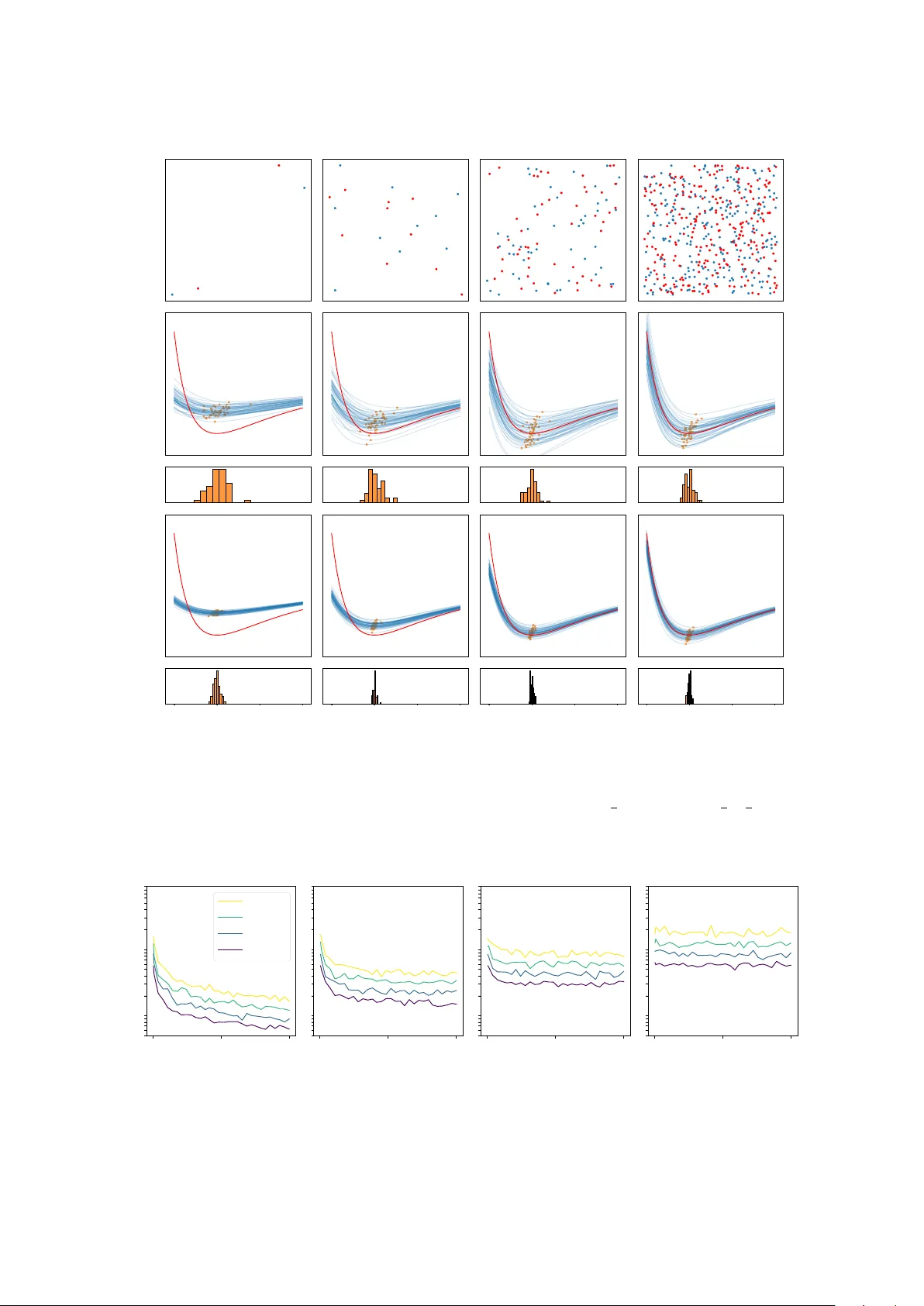
Densit y estimation from batc hed brok en random samples Hanc heng Bi, Bernhard Sc hmitzer, Thilo D. Stier F ebruary 11, 2026 Abstract The br oken r andom sample problem w as first in tro duced b y DeGro ot, F eder, and Gole (1971, Ann. Math. Statist.): in each observ ation (batch), a random sample of M i.i.d. p oin t pairs (( X i , Y i )) M i =1 is dra wn from a joint distribution with density p ( x, y ), but w e can observ e only the unordered multisets ( X i ) M i =1 and ( Y i ) M i =1 separately; that is, the pairing information is lost. F or large M , inferring p from a single observ ation has been sho wn to b e essentially imp ossible. In this pap er, w e propose a parametric metho d based on a pseudo-log-likelihoo d to estimate p from N i.i.d. broken sample batches, and we pro ve a fast conv ergence rate in N for our estimator that is uniform in M , under mild assumptions. 1 In tro duction 1.1 Problem statemen t and related work Problem statemen t. Let X , Y be measurable spaces and π ∈ P ( X × Y ) b e a join t probability measure. Let ( X i , Y i ) M i =1 b e indep enden t and identically distributed (i.i.d.) pairs of random v ariables with law π . W e assume that w e do not hav e access to the actual pairing information, i.e. w e will only observe the random multisets { X 1 , · · · , X M } and { Y 1 , · · · , Y M } but not the ordering of the points. This is called a br oken r andom sample from π , originally introduced in [ 7 ]. Previous researc h on extracting information from a broken sample when π is a bi-v ariate normal distribution includes [ 8 ] and [ 5 ]. In particular, [ 3 ] pro ved that estimating the correlation parameter is not p ossible under some mild conditions. In this pap er w e assume that instead of observing a single broken sample, we ha ve access to N i.i.d. observ ations of broken samples, i.e. w e hav e i.i.d. pairs of random v ariables (( X k i , Y k i ) M i =1 ) N k =1 with law π and we observ e the collection of multisets  { X k 1 , · · · , X k M } , { Y k 1 , · · · , Y k M }  N k =1 . W e are in terested in estimating π in a parametric setting from these i.i.d. samples and inv estigate the b eha viour of the estimator with respect to N and M . W e refer to each observ ed pair of multisets ( { X k 1 , · · · , X k M } , { Y k 1 , · · · , Y k M } ) as a b atch and to the problem of estimating π as the b atche d br oken sample pr oblem . If M = 1 w e recov er the classical problem of estimating π from N i.i.d. samples. Ho wev er, due to the missing pairing information, as M → ∞ , intuitiv ely the batc hes will b e approximately indep endent samples from the marginal distributions of π , which leads to the suspicion that the information about π carried b y each batc h could decrease to zero as M increases. In the following w e prov e that this is not the case. Applications. The batched brok en sample problem serves as a idealised mo del for particle colocalisa- tion analysis. Figure 1 shows part of a sup er-resolution fluorescence microscop y image of immunolabelled h uman cells. The HA-tag in the mito chondrial outer membrane and the protein Mic60 in the mito c hon- drial inner mem brane are tagged with green and purple markers, respectively . Most proteins app ear to b e lo cated within close spatial proximit y of a protein from the other sp ecies. Is this b ecause the proteins form b ound pairs to realize their biological function, or are the protein lo cations indep enden t from each other and colocalisation is merely accidental, stemming from the high density of particles in a confined 1 Figure 1: Stimulated emission depletion (STED) microscopy image, part of [ 9 , Fig 37(A)]. Cells were stained for the HA-tag (green) and Mic60 (purple). region? If one mo dels the protein locations of the t wo sp ecies as random v ariables X i and Y i , as ab o ve, then the t wo situations can b e distinguished, based on the law of π : F or bound pairs, X i and Y i will b e close with high probability; in the case of accidental colo calisation, π is an indep endent product measure. Of course, to realistically estimate π from images one must take in to accoun t several additional effects: not all particles are actually captured in the imaging pro cess; even when particles do tend to form pairs, not all particles are necessarily paired at all times; and particles in differen t images will follow sligh tly differen t la ws π . How ever, our simplified model does demonstrate that increasing particle densit y is not necessarily a problem for inferring π . Another application is the analysis of time-discrete dynamical systems. In this case we interpret X i and Y i as p ositions of a particle at tw o subsequen t time steps and a common task is to infer the conditional distribution of Y i , giv en X i . M = 1 corresp onds to observing the evolution of a single particle whereas M > 1 corresp onds to the case where w e observe multiple indistinguishable particles, such as floaters in a fluid as in particle image v elo cimetry , where small particles are seeded in to the fluid and illuminated b y a pulsed laser. The distribution of light scattered by these particles is recorded eac h time the laser pulses, thereb y creating a discrete sequence of images (see, e.g., [ 1 , Fig. 6]). The task is to retrieve the flo w v elo cit y . When the p oin t density is relatively low, or when p oin ts mo ve slowly , b oth of the ab ov e problems can b e tac kled using optimal-transp ort-based metho ds; see [ 11 ] and [ 1 , 10 ], resp ectiv ely . How ever, optimal transp ort tends to bias the pairing tow ards coincidentally close p oin ts, which b ecomes more likely as the p oin t density increases. In this pap er, we in tro duce a parametric metho d to estimate the density of the la w π , and we prov e quantitativ ely that the metho d is not affected in the high-density regime (i.e. as M → ∞ ). A non-parametric metho d using a similar loss function has b een discussed in [ 4 ], along with a qualitativ e proof of con v ergence as N → ∞ in a suitable sense. 1.2 Outline Throughout the rest of this section we in tro duce assumptions and notation, state the problem in detail and preview the main results. In Section 2 we collect or prov e necessary auxiliary theorems and lemmata. Our main results are prov en in Section 3 . Some numerical illustrations are sho wn in Section 4 . 1.3 Problem description and main results Let µ ∈ P ( X ) and ν ∈ P ( Y ) b e the marginal distributions of π . In a setting where π can b e identified from the marginals, the problem reduces to con ven tional density estimation. Therefore, throughout this pap er, w e alw ays assume µ, ν are known, and we are interested in estimating the densit y of π with resp ect to µ ⊗ ν , analogous to [ 3 , p. 529]. In practice one ma y first estimate µ and ν with v ery high precision from the M · N i.i.d. random v ariables ( X k i ) i,k and ( Y k i ) i,k . Assumption 1.1. π = p ∗ · ( µ ⊗ ν ) for some p ∗ : X × Y → R . W e also need to define a candidate set from which we pic k the estimator. Here we use a parametric class. Definition 1.2. L et Θ b e an op en subset of finite dimensional Euclide an sp ac e with c omp act closur e ¯ Θ , let D := sup θ,θ ′ ∈ Θ ∥ θ − θ ′ ∥ b e its diameter. L et ( p θ ) θ ∈ ¯ Θ b e a p ar ametric class of densities with the fol lowing pr op erties: 2 1. The set of functions { ¯ Θ ∋ θ 7→ p θ ( x, y ) | ( x, y ) ∈ X × Y } is twic e c ontinuously differ entiable when r estricte d to Θ , e quib ounde d by some c onstant 0 < U < ∞ , e qui-Lipschitz with some Lipschitz c onstant L < ∞ , and al l dir e ctional derivatives of se c ond or der with r esp e ct to θ ∈ Θ ar e e quib ounde d by L ′ < ∞ . 2. F or al l θ ∈ Θ , x ∈ X , y ∈ Y , we have R X p θ ( x ′ , y )d µ ( x ′ ) = R Y p θ ( x, y ′ )d ν ( y ′ ) = 1 . Remark 1.3 (Breaking the samples) . In or der to ‘for get’ the p airing information within b atches, the authors of [ 4 ] intr o duc e d an auxiliary r andom variable, a uniformly sample d p ermutation σ ∼ U ( Sym ( M )) , and assume that, for e ach b atch one c an only observe (( X i , Y σ ( i ) )) M i =1 . As discusse d in [ 4 ], in this mo del the ne gative lo g-likeliho o d is given by ℓ ( θ ) = − 1 N N X k =1 log 1 M ! X σ ∈ S M M Y i =1 p θ  X k i , Y k σ ( i )  ! . (1) While this is a rigor ous way to formulate the br oken-sample pr oblem, it intr o duc es an extr a r andom variable and c omplic ates the pr ob ability sp ac e. In this p ap er, we take a differ ent appr o ach for the sake of simplicity: Inste ad of explicitly mo del ling the br oken samples (e.g. by applying an unknown uniformly r andom p ermutation to the p oints), we mo del the data with a known p airing but make sur e that our estimator do es not use any p airing information. Explicitly this emer ges as the estimator b eing define d as the minimiser of a loss function which is invariant under within-b atch p ermutation of the p oints. Clearly , Equation ( 1 ) is permutation inv ariant and therefore in principle it can b e used as loss function. Ho wev er it is not feasible in practice unless M is very small, since the complexity of ev aluation of ℓ ( θ ) is in general NP-hard [ 12 ]. Inspired b y [ 4 ], we define our loss function through a negativ e pseudo log-lik eliho od f N M ( θ ) := − 1 N N X k =1 M X i =1 M X j =1 log  1 M p θ ( X k i , Y k j ) + M − 1 M  and its minimiser θ N M ∈ argmin θ ∈ ¯ Θ f N M ( θ ) . (2) In addition, we introduce f M ( θ ) := E ( f N M ( θ )) , f ∞ ( θ ) := lim M →∞ f M ( θ ) , θ M ∈ argmin θ ∈ ¯ Θ f M ( θ ) , θ ∞ ∈ argmin θ ∈ ¯ Θ f ∞ ( θ ) . A t first glance, one might susp ect that f N M scales as O ( M 2 ) as M → ∞ b ecause of the double sum o ver i and j . This concern is resolv ed by Theorem 1.6 , which shows that the exp ectation f M ( θ ) has a finite limit as M → ∞ . Remark 1.4. Intuitively the ne gative pseudo-lo g-likeliho o d ( 2 ) arises as fol lows. When uniformly cho os- ing a r andom p air ( i, j ) of p oint indic es in some b atch k , ther e is a 1 M chanc e that X := X k i and Y := Y k j form a p air with distribution π and a M − 1 M chanc e that they ar e indep endent, i.e. ( X , Y ) ∼  1 M p ∗ + M − 1 M  ( µ ⊗ ν ) . Differ ent p airs ( X k i , Y k j ) (for the same k , but differ ent i, j ) wil l in gener al not b e indep endent fr om e ach other. However, if we al low for this appr oximation, ( 2 ) arises as the sum of the (ne gative) lo g-likeliho o ds of al l p airs. Remark 1.5 (Comparison with [ 4 ]) . In [ 4 ] the fol lowing pseudo-likeliho o d θ 7→ − 1 N N X k =1 M X j =1 log 1 M M X i =1 p θ ( X k i , Y k j ) ! (3) is c onsider e d inste ad of ( 2 ) . This is also p ermutation invariant. The term 1 M P M i =1 p θ ( X k i , Y k j ) app e aring within the lo garithm c orr esp onds to the c onditional pr ob ability of Y k j , c onditione d on the tuple ( X k i ) M i =1 , if one assumes that the p airing information is unavailable. ( 3 ) then arises by ar guing analo gously to R emark 1.4 by making the appr oximation that the variables ( Y k j ) M j =1 ar e indep endent, when c onditione d on ( X k i ) M i =1 . Using te chniques fr om [ 4 ] it c an b e ar gue d that ( 3 ) is a mor e ac cur ate appr oximation than ( 2 ) , however we c onsider the latter in this manuscript as it is mor e amenable to quantitative c onver genc e analysis. 3 W e can now state our main results. The first result is on the asymptotic form of the exp ected pseudo lik eliho o d as M → ∞ . Theorem 1.6. f M ( θ ) = f ∞ ( θ ) + O ( M − 1 ) wher e f ∞ ( θ ) = 1 2    p θ − p ∗   2 L 2 ( µ ⊗ ν ) − ∥ p ∗ ∥ 2 L 2 ( µ ⊗ ν ) + 1  . Remark 1.7 (Behaviour of minimizers of f M ) . When M = 1 , f M r e duc es to the standar d p opulation ne g- ative lo g-likeliho o d. It is wel l known that minimising the ne gative lo g-likeliho o d is e quivalent to minimising the KL diver genc e b etwe en the true distribution and our estimate d one. F or arbitr ary M , analo gously to [ 4 , Pr op osition A.4], we have f M ( θ ) = M 2 · KL  ( 1 M p ∗ + M − 1 M ) · µ ⊗ ν   ( 1 M p θ + M − 1 M ) · µ ⊗ ν  + const . This fol lows fr om Equation ( 5 ) in the pr o of of The or em 1.6 . Henc e, if p ∗ ∈ ( p θ ) θ ∈ Θ , we c onclude that any minimiser of f M e quals p ∗ µ ⊗ ν -almost everywher e. If p ∗ / ∈ ( p θ ) θ ∈ Θ , then for M = 1 , minimizers of f M wil l b e KL-pr oje ctions of p ∗ onto the p ar ametric class. By The or em 1.6 , as M → ∞ minimizers of f M should c onver ge to the L 2 ( µ ⊗ ν ) -pr oje ction. This b e c omes mor e c oncr ete in The or em 1.9 . The next result is on the concentration of f N M around f M , uniformly in θ . Theorem 1.8. L et D , U, L b e as in Definition 1.2 , let J := Z D 0 log (1 + N ( ε ; Θ , ∥·∥ )) d ε < ∞ , in which N ( ε ; Θ , ∥·∥ ) is the c overing numb er of (Θ , ∥·∥ ) with r adius ε . Note that J is finite under our assumption for Θ . Then ther e exists an absolute c onstant c > 0 such that P  sup θ ∈ Θ   f N M ( θ ) − f M ( θ )   ≥ 6 t  ≤ 6 exp  − c min n t 2 N U 4 , tN U o  + 6 exp  J D  exp − ct √ N D L U ! for al l t > 0 . This suggests that the estimation qualit y will benefit from large N as exp ected and will not b e harmed b y large M . Instead, in com bination with Theorem 1.6 , for large M and N w e see that one can exp ect the estimator of p ∗ to be close to the L 2 ( µ ⊗ ν )-pro jection of p ∗ on to ( p θ ) θ ∈ ¯ Θ . As a consequence, when assuming uniqueness of this pro jection and strictly p ositiv e curv ature of ∥ p θ − p ∗ ∥ 2 L 2 ( µ ⊗ ν ) around it, one can get a lo w er b ound of the con v ergence rate of the minimiser of f N M ( θ ) to the minimiser of f M ( θ ) for large M : Theorem 1.9. Assume that θ ∞ ∈ Θ is the unique minimiser of f ∞ , and ther e exist some τ , r > 0 such that the smal lest eigenvalue of ∇ 2 f ∞ ( θ ) is lar ger than τ for al l θ ∈ Θ with ∥ θ − θ ∞ ∥ 2 ≤ r . Then ther e exist some M 0 ∈ N , t 0 > 0 s.t. for al l M ≥ M 0 and t ≤ t 0 we have P    θ N M − θ M   2 ≥ t  ≤ C 1 exp  − C 2 min n t 2 N , t √ N o , wher e the empiric al minimizer θ M is unique and C 1 , C 2 > 0 ar e c onstants indep endent of M and N . 4 2 Preliminaries Theorem 2.1 (Differentiabilit y of parametrised integrals [ 2 , Theorem 3.18]) . Supp ose Θ is op en in R n , and supp ose f : X × Θ → R satisfies 1. f ( · , θ ) ∈ L 1 µ ( X ) for every θ ∈ Θ ; 2. f ( x, · ) ∈ C 1 (Θ) for µ -almost every x ∈ X ; 3. ther e exists some g ∈ L 1 µ ( X ) such that    ∂ ∂ θ m f ( x, θ )    ≤ g ( x ) for al l ( x, θ ) ∈ X × Θ and m ∈ { 1 , . . . , n } . Then θ 7→ R X f ( x, θ )d µ is c ontinuously differ entiable and ∂ ∂ θ m Z X f ( x, θ )d µ ( x ) = Z X ∂ ∂ θ m f ( x, θ )d µ ( x ) for al l θ ∈ Θ and m ∈ { 1 , . . . , n } . Definition 2.2 ( ψ 1 -norm) . [ 13 , e qn. (2.21)] The sub-exp onential norm of a r e al value d r andom variable F is define d by ∥ F ∥ ψ 1 = inf  t > 0 : E exp  | F | t  ≤ 2  . Lemma 2.3. Given a r andom variable F with E ( | F | p ) ≤ ( C p ) p for al l p ∈ N , we have ∥ F ∥ ψ 1 ≤ 2 eC . Pr o of. Substitute t = 2 eC into the following equation E exp  | F | t  = E ∞ X p =0 | F | p t p p ! ! ≤ ∞ X p =0 C p p p t p p ! ≤ ∞ X p =0 C p e p t p = 1 1 − C e t where we used ( p/e ) p ≤ p ! as w ell as the limit of the geometric series. Theorem 2.4 (Bernstein, Corollary 2.8.3 in [ 13 ]) . L et F 1 , ..., F N b e i.i.d. sub-exp onential r andom vari- ables with me an zer o, then for any t ≥ 0 we have P      1 N N X i =1 F i      ≥ t ! ≤ 2 exp − c min ( t 2 N ∥ F 1 ∥ 2 ψ 1 , tN ∥ F 1 ∥ ψ 1 )! in which c is an absolute c onstant. Lemma 2.5. L et F 1 , ..., F N b e i.i.d. sub-exp onential r andom variables with me an zer o, then for some absolute c onstant c > 0 we have      1 N N X i =1 F i      ψ 1 ≤ c ∥ F 1 ∥ ψ 1 √ N . Pr o of. Denote β := ∥ F 1 ∥ ψ 1 . F or an y p ≥ 1, by Theorem 2.4 E      1 N N X i =1 F i      p ! = Z ∞ 0 P      1 N N X i =1 F i      p ≥ t ! d t = p Z ∞ 0 P      1 N N X i =1 F i      ≥ t ! t p − 1 d t ≤ 2 p Z ∞ 0 t p − 1 exp  − cN t 2 β 2  d t + 2 p Z ∞ 0 t p − 1 exp  − cN t β  d t ≤ 2 p  cN β 2  − p/ 2 Γ  p 2  + 2 p  cN β  − p Γ( p ) ≤ 6 p Γ( p )  β c √ N  p ≤  6 β p c √ N  p . 5 In the last line w e used that the c from Theorem 2.4 w.l.o.g. fulfills c ≤ 1 and that for p ≥ 1 we hav e Γ( p/ 2) ≤ 2Γ( p ) as w ell as p Γ( p ) = p ! ≤ p p . Applying Lemma 2.3 finishes the proof. Definition 2.6 ( ψ 1 -pro cess, Definition 5.35 in [ 14 ]) . A zer o me an sto chastic pr o c ess { F θ : θ ∈ Θ } is a ψ 1 pr o c ess with r esp e ct to a norm ∥·∥ Θ if ∥ F θ − F θ ′ ∥ ψ 1 ≤ ∥ θ − θ ′ ∥ Θ . Lemma 2.7. Consider a p ar ametric class of functions g θ : X → R , a pr ob ability me asur e ρ ∈ P ( X ) , and some i.i.d. X k ∼ ρ . If ther e exists an L > 0 such that for any θ, θ ′ ∈ Θ one has    g θ − g θ ′    ∞ ≤ L ∥ θ − θ ′ ∥ Θ , then F N ( θ ) := 1 N N X k =1 g θ ( X k ) − E g θ ( X ) is a ψ 1 -pr o c ess with r esp e ct to the norm cL √ N ∥·∥ Θ for an absolute c onstant c > 0 . Pr o of. Note that E ( | F 1 ( θ ) − F 1 ( θ ′ ) | p ) ≤ (2 L ∥ θ − θ ′ ∥ ) p , apply Lemma 2.3 and Lemma 2.5 . Definition 2.8 (Generalized Dudley entrop y integral) . T ake D fr om Definition 1.2 . We define J ( δ, D ) = Z D δ log  1 + N ( ε ; Θ , ∥·∥ Θ )  d ε wher e N ( ε ; Θ , ∥·∥ Θ ) is the ε -c overing numb er for (Θ , ∥·∥ Θ ) . Theorem 2.9 (Theorem 5.36 in [ 14 ]) . L et { F θ : θ ∈ Θ } b e a ψ 1 -pr o c ess with r esp e ct to ∥·∥ Θ , then ther e is a universal c onstant c 1 such that for al l t ∈ R we have P sup θ,θ ′ ∈ Θ | F θ − F θ ′ | ≥ c 1 ( J (0 , D ) + t ) ! ≤ 2 exp  − t D  . Lemma 2.10. T ake D fr om Definition 1.2 , and let ∥·∥ denote the standar d Euclide an norm. Define J := Z D 0 log (1 + N ( ε ; Θ , ∥·∥ )) d ε. L et f ( θ ) b e a ψ 1 -pr o c ess w.r.t. C √ N ∥·∥ for some C > 0 . Ther e is an absolute c onstant c 1 > 0 such that for al l t > 0 P sup θ,θ ′ ∈ Θ | f ( θ ) − f ( θ ′ ) | ≥ t ! ≤ 2 exp  J D  exp − t √ N c 1 D C ! . Pr o of. First note that since ¯ Θ is a compact subspace of finite dimensional Euclidean space, we ha ve J < ∞ b y [ 6 , Prop osition 5]. Let D ′ := sup θ,θ ′ ∈ Θ C √ N ∥ θ − θ ′ ∥ = DC √ N . F rom Definition 2.8 , using a c hange of v ariables in the in tegral we get J (0 , D ′ ) = Z D ′ 0 log  1 + N  ε ; Θ , C √ N ∥·∥   d ε = C J √ N . (4) By Theorem 2.9 w e hav e for some absolute constant c 1 > 0 P sup θ,θ ′ ∈ Θ | f ( θ ) − f ( θ ′ ) | ≥ c 1  C J √ N + τ  ! ≤ 2 exp  − τ D ′  = 2 exp  − τ √ N D C  ∀ τ ∈ R . Substituting t = c 1  C J √ N + τ  finishes the pro of. 6 Lemma 2.11. L et { F θ : θ ∈ Θ } b e a sto chastic pr o c ess and fix some θ 0 ∈ Θ . Then P  sup θ ∈ Θ | F θ | ≥ 2 t  ≤ P sup θ,θ ′ ∈ Θ | F θ − F θ ′ | ≥ t ! + P ( | F θ 0 | ≥ t ) . Pr o of. Apply triangle inequality and union b ound. Lemma 2.12 (Ho effding, Theorem 2.2.6 in [ 13 ]) . L et F 1 , ..., F N b e i.i.d., assume that | F k | ≤ C , then for any t ≥ 0 , we have P      1 N N X k =1 F k − E ( F 1 )      ≥ t ! ≤ 2 exp  − N t 2 2 C 2  . 3 Non-asymptotic con v ergence results 3.1 Concen tration of f N M ( θ ) F rom no w on w e assume M ≥ 2. In this section we will abbreviate the random v ariables p θ ( X k i , Y k j ) as p k ij ( θ ). Similarly , for points ( x i ) i ⊂ X , ( y i ) i ⊂ Y , we abbreviate p ∗ ( x i , y i ) as p ∗ ii and p θ ( x i , y j ) as p ij ( θ ). W e also define q k ij ( θ ) := p k ij ( θ ) − 1 and q ij ( θ ) = p ij ( θ ) − 1. Note that p ∗ ii and p ij in tegrate to 1 on b oth marginals, i.e. we hav e Z X p ∗ ii d µ ( x i ) = Z X p ∗ ii d ν ( y i ) = 1 and a corresp onding statement for p ij ( θ ). Similarly q ij ( θ ) integrates to 0. W e write d π ii for integrating against d π ( x i , y i ) and d π ⊗ M for the joint integration against all factors Π M i =1 d π ii . W e use similar notation for integrals against the product measure µ ⊗ ν . W e now prov e a statement ab out the asymptotic form of our expected pseudo-likelihoo d, as M → ∞ . Theorem (Recollection of Theorem 1.6 ) . f M ( θ ) = 1 2    p θ − p ∗   2 L 2 ( µ ⊗ ν ) − ∥ p ∗ ∥ 2 L 2 ( µ ⊗ ν ) + 1  + O ( M − 1 ) . Pr o of. Recall q ij ( θ ) := p ij ( θ ) − 1. W e get − f M ( θ ) = Z M X i,j =1 log  1 M p ij ( θ ) + M − 1 M  d π ⊗ M = Z M X i,j =1 log  1 + 1 M q ij ( θ )  M Y l =1 p ∗ ll d( µ ⊗ ν ) ⊗ M = M X i =1 Z log  1 + 1 M q ii ( θ )  M Y l =1 p ∗ ll d( µ ⊗ ν ) ⊗ M + X i  = j Z log  1 + 1 M q ij ( θ )  M Y l =1 p ∗ ll d( µ ⊗ ν ) ⊗ M . F or the first part, consider the summand i = 1. It equals R log(1 + q 11 / M ) p ∗ 11 Q l  =1 p ∗ ll d( µ ⊗ ν ) ⊗ M , and one can integrate ov er ( x l , y l ) for all l  = 1 b y using R p ∗ ll dµ ⊗ ν = 1. One can argue likewise for all other v alues of i , yielding M times the same v alue. F or the second part, similarly consider the summand i = 1 and j = 2. It equals R log(1 + q 12 / M ) p ∗ 11 p ∗ 22 Q M l =3 p ∗ ll d( µ ⊗ ν ) ⊗ M , we can again in tegrate o ver ( x l , y l ) for l ≥ 3, and then integrate ov er y 1 and x 2 b y R X p ∗ 22 d µ ( x 2 ) = R Y p ∗ 11 d ν ( y 1 ) = 1. Arguing likewise for all other v alues of i, j , one obtains M ( M − 1) times this contribution. Therefore, − f M ( θ ) = M Z log  1 + 1 M q 11 ( θ )  p ∗ 11 d µ ⊗ ν + M ( M − 1) Z log  1 + 1 M q 11 ( θ )  d µ ⊗ ν = M 2 Z log  1 + 1 M q 11 ( θ )   1 M p ∗ 11 + M − 1 M  d µ ⊗ ν . (5) 7 Next, we derive the asymptotic b eha viour as M → ∞ . F or this we use the T aylor expansion log (1 + x ) = x − x 2 / 2 + O ( x 3 ) (with the fact that q 11 ( θ ) ∈ [ − 1 , U − 1], making the approximation error uniformly b ounded) and M ≥ 2 to obtain − f M ( θ ) = M 2 Z  q 11 ( θ ) M − ( q 11 ( θ )) 2 2 M 2 + O ( M − 3 )  1 M p ∗ 11 + M − 1 M  d µ ⊗ ν = M 2 Z q 11 ( θ ) M 1 M p ∗ 11 + q 11 ( θ ) M ( M − 1) M − ( q 11 ( θ )) 2 2 M 2  1 M p ∗ 11 + ( M − 1) M  d µ ⊗ ν + O ( M − 1 ) . W e contin ue by cancelling the second term via R q 11 d µ ⊗ ν = 0, absorbing more terms in to the O ( M − 1 ) and rearranging the rest − f M ( θ ) = 1 2 Z 2 q 11 ( θ ) p ∗ 11 − ( q 11 ( θ )) 2  1 M p ∗ 11 + ( M − 1) M  d µ ⊗ ν + O ( M − 1 ) = 1 2 Z 2 q 11 ( θ ) p ∗ 11 − ( q 11 ( θ )) 2 d µ ⊗ ν + O ( M − 1 ) = − 1 2 Z  q 11 ( θ ) − p ∗ 11  2 d µ ⊗ ν + 1 2 Z ( p ∗ 11 ) 2 d µ ⊗ ν + O ( M − 1 ) . No w w e re-substitute q 11 = p 11 + 1 to finish the proof − f M ( θ ) = − 1 2 Z  p 11 ( θ ) − p ∗ 11  2 − 2  p 11 ( θ ) − p ∗ 11  + 1 d µ ⊗ ν + 1 2 Z ( p ∗ 11 ) 2 d µ ⊗ ν + O ( M − 1 ) = − 1 2 Z  p 11 ( θ ) − p ∗ 11  2 d µ ⊗ ν + 1 2 Z ( p ∗ 11 ) 2 d µ ⊗ ν − 1 2 + O ( M − 1 ) . Theorem (Recollection of Theorem 1.8 ) . L et J, D b e as in L emma 2.10 . Ther e exists an absolute c onstant c > 0 such that P  sup θ ∈ Θ   f N M ( θ ) − f M ( θ )   ≥ 6 t  ≤ 6 exp  − c min n t 2 N U 4 , tN U o  + 6 exp  J D  exp − ct √ N D L U ! . The full pro of will b e provided at the end of this section. T o control sup θ ∈ Θ   f N M ( θ ) − f M ( θ )   w e separate f N M ( θ ) into three terms, namely f N M ( θ ) = 1 N M N X k =1 M X i,j =1 q k ij ( θ ) + f N M ( θ ) − 1 N M N X k =1 M X i,j =1 q k ij ( θ ) = − 1 N M N X k =1 M X i,j =1 ,i  = j q k ij ( θ ) | {z } f a ( θ ) − 1 N M N X k =1 M X i =1 q k ii ( θ ) | {z } f b ( θ ) + f N M ( θ ) + 1 N M N X k =1 M X i,j =1 q k ij ( θ ) | {z } f c ( θ ) (6) and apply the triangle inequality to get sup θ ∈ Θ   f N M ( θ ) − f M ( θ )   ≤ sup θ ∈ Θ | f a ( θ ) − E f a ( θ ) | + sup θ ∈ Θ | f b ( θ ) − E f b ( θ ) | + sup θ ∈ Θ | f c ( θ ) − E f c ( θ ) | . (7) Our goal is to obtain an M -indep enden t concentration rate for f N M , and we separate f N M in to three parts for a cleaner presentation. Note that the concentration of f a requires more effort than the others, since it is the component that naiv ely app ears to scale at the rate O ( M ). The follo wing lemmata work tow ards b ounding each of the summands abov e. Lemma 3.1 (Com binatorial interlude) . L et l ∈ N , and we write J 1 , l K := { 1 , . . . , l } for the first l natur al numb ers. Define S := { ( z i ) 2 l i =1 ∈ J 1 , M K 2 l | ∀ i ∃ j  = i : z j = z i } . 8 This c an b e interpr ete d as the set of strings over the alphab et J 1 , M K of length 2 l wher e no char acter app e ars exactly onc e. We have | S | ≤ (2 M l ) l . Pr o of. Let B := { b := ( b i ) 2 l i =1 ∈ { 0 , 1 } 2 l | ∥ b ∥ 1 = l } b e the set of binary strings of length 2 l with exactly l en tries equal to 1. W e define a map σ : B × J 1 , M K l × J 1 , l K l → S, ( b, c, k ) 7→ s b y the following pro cedure: • F or i ∈ J 1 , l K , let j b e the i -th entry in b equal to 1. Set s j := c i . • F or i ∈ J 1 , l K , let j b e the i -th entry in b equal to 0. Set s j := c k i . Next we sho w that σ is surjective and the preimage of an y s ∈ S has at least 2 l elemen ts. Giv en an arbitrary s ∈ S , let τ b e a p erm utation such that ( s τ ( i ) ) 2 l i =1 starts with a pair of each letter occurring in s follo wed b y the rest in arbitrary order. This exists since no letter app ears exactly once in s . In the following, w e assume w.l.o.g. τ = id. W e construct preimages of s ∈ S under σ by the follo wing pro cedure: • F or i ∈ J 1 , l K set ( b 2 i − 1 , b 2 i ) ∈ { (1 , 0) , (0 , 1) } arbitrarily . • F or i ∈ J 1 , l K set c i := ( s 2 i − 1 if b 2 i − 1 = 1 , s 2 i if b 2 i = 1 . • F or i ∈ J 1 , l K set k i := ( c − 1 ( s 2 i − 1 ) if b 2 i − 1 = 0 , c − 1 ( s 2 i ) if b 2 i = 0 where c − 1 ( a ) denotes an arbitrary index j ∈ J 1 , l K such that c j = a (whic h exists by assumption and construction). Applying the pro cedure defining σ to this, it is easy to see that the constructed v alues are indeed preimages and since ( b 2 i − 1 , b i ) are chosen independently and arbitrarily from t wo possibilities each, we ha ve 2 l differen t preimages. Therefore | S | ≤ | B | M l l l 2 l ≤ 2 2 l M l l l 2 l = (2 M l ) l . Lemma 3.2. f a ( θ ) is a ψ 1 -pr o c ess with r esp e ct to c L √ N ∥·∥ , in which c > 0 is some absolute c onstant and ∥·∥ is the original norm on Θ . Pr o of. Let F k ( θ ) := 1 M P M i  = j q k ij ( θ ), then f a ( θ ) = 1 N P N k =1 F k ( θ ). Note that F k ( θ ) has mean E F k ( θ ) = 1 M M X i  = j Z q ij M Y m =1 p ∗ mm d( µ ⊗ ν ) ⊗ M = 1 M M X i  = j Z q ij d( µ ⊗ ν ) ⊗ M = 0 . F or even l ∈ N we get E  | F 1 ( θ ) − F 1 ( θ ′ ) | l  = E  ( F 1 ( θ ) − F 1 ( θ ′ )) l  = 1 M l M X i 1  = j 1 · · · M X i l  = j l E l Y α =1  q 1 i α j α ( θ ) − q 1 i α j α ( θ ′ )  ! . W e examine the exp ectation term. By definition we hav e E l Y α =1  q 1 i α j α ( θ ) − q 1 i α j α ( θ ′ )  ! = Z l Y α =1 ( q i α j α ( θ ) − q i α j α ( θ ′ )) M Y m =1 p ∗ mm d( µ ⊗ ν ) ⊗ M . 9 Giv en a set of indices as ab ov e, if there exists some i β that is unique, i.e. i β ∈ { i α | α : α  = β } ∪ { j α | α } , w e can first perform the integral ov er y i β (whic h only app ears in the p ∗ -term, yielding 1) and then perform the integral o ver x i β (whic h only app ears in one q -term, yielding 0). This factor then implies that the whole integral is 0. Similarly , if there is some unique j β , the integral is 0. W e conclude that if there exists an y v alue that only app ears once in ( i 1 , · · · , i l , j 1 , · · · , j l ) then the integral is zero. Using S, L as defined in Lemma 3.1 and Definition 1.2 together with the equations ab o ve, w e get E  | F 1 ( θ ) − F 1 ( θ ′ ) | l  ≤ 1 M l | S | sup x,y    q θ ( x, y ) − q θ ′ ( x, y )    l ≤ 1 M l | S | L l ∥ θ − θ ′ ∥ l ≤ (2 L ∥ θ − θ ′ ∥ l ) l . No w for l ∈ N b eing o dd, apply Jensen’s inequalit y E  | F 1 ( θ ) − F 1 ( θ ′ ) | l  ≤  E  | F 1 ( θ ) − F 1 ( θ ′ ) | l +1  l l +1 ≤ (2 L ∥ θ − θ ′ ∥ ( l + 1)) l ≤ (4 L ∥ θ − θ ′ ∥ l ) l . By Lemma 2.3 w e hav e ∥ F 1 ( θ ) − F 1 ( θ ′ ) ∥ ψ 1 ≤ 8 e L ∥ θ − θ ′ ∥ . Since F k are i.i.d. and f a ( θ ) = 1 N P N k =1 F k , b y Lemma 2.5 w e hav e ∥ f a ( θ ) − f a ( θ ′ ) ∥ ψ 1 ≤ c L √ N ∥ θ − θ ′ ∥ for some absolute constant c > 0. Lemma 3.3. f b ( θ ) − E f b ( θ ) is a ψ 1 -pr o c ess with r esp e ct to c L √ N ∥·∥ for some absolute c onstant c > 0 . Pr o of. Note that    1 M P M i =1  q 1 ii ( θ ) − q 1 ii ( θ ′ )     ≤ L ∥ θ − θ ′ ∥ and apply Lemma 2.7 . Lemma 3.4. f c ( θ ) − E f c ( θ ) is a ψ 1 -pr o c ess with r esp e ct to c L U √ N ∥·∥ for some absolute c onstant c > 0 . Pr o of. W e hav e ∇ θ M X i,j =1 log  1 M p 1 ij ( θ ) + M − 1 M  − ∇ θ 1 M M X i,j =1 q 1 ij ( θ ) = M X i,j =1 1 M ∇ θ p 1 ij ( θ ) 1 M p 1 ij ( θ ) + M − 1 M − 1 M ∇ θ p 1 ij ( θ ) ! = 1 M 2 M X i,j =1 (1 − p 1 ij ( θ )) ∇ θ p 1 ij ( θ ) 1 M p 1 ij ( θ ) + M − 1 M . Using the assumption M ≥ 2, this implies       −∇ θ M X i,j =1 log  1 M p 1 ij ( θ ) + M − 1 M  + ∇ θ 1 M M X i,j =1 q 1 ij ( θ )       2 ≤ 2 L U. Applying Lemma 2.7 finishes the proof. Lemma 3.5. F or fixe d θ 0 ∈ Θ , ther e is an absolute c onstant c > 0 such that P ( | f a ( θ 0 ) | ≥ t ) ≤ 2 exp  − c min n t 2 N U 2 , tN U o  . Pr o of. The pro of work s very similarly to that of Lemma 3.2 . Let F k ( θ 0 ) = 1 M P i  = j q k ij ( θ 0 ). F or even l ∈ N we get E  | F 1 ( θ 0 ) | l  = 1 M l X i 1  = j 1 · · · X i l  = j l E l Y α =1 q 1 i α j α ! ≤ 2 l sup x,y ,θ   p θ ( x, y ) − 1   ! l ≤ (2 l U ) l . Using Jensen to get the b ound for o dd l , then by Lemma 2.3 w e hav e ∥ F 1 ∥ ψ 1 ≤ 8 eU . Now apply Theorem 2.4 to finish the proof. Lemma 3.6. F or fixe d θ 0 ∈ Θ we have P ( | f b ( θ 0 ) − E f b ( θ 0 ) | ≥ t ) ≤ 2 exp  − t 2 N 2 U 2  . 10 Pr o of. Note that    1 M P M i =1 q 1 ii ( θ )    ≤ sup x,y ,θ   p θ ( x, y ) − 1   ≤ U . Apply Lemma 2.12 . Lemma 3.7. F or fixe d θ 0 ∈ Θ we have P ( | f c ( θ 0 ) − E f c ( θ 0 ) | ≥ t ) ≤ 2 exp  − t 2 N 8 U 4  . Pr o of. Note that for an y x > 0 there is a ξ = ξ ( x ) betw een 1 and 1 + x such that log(1 + x ) = x − x 2 2 ξ 2 . Therefore       M X i,j =1  log  1 + 1 M q 1 ij ( θ )  − 1 M q 1 ij ( θ )        =       1 2 M 2 M X i,j =1 ( q 1 ij ( θ )) 2 ξ 2       ≤ 2 sup x,y ,θ   p θ ( x, y ) − 1   2 ≤ 2 U 2 in which ξ is b et w een 1 and 1 + 1 M q 1 ij , and since M ≥ 2 we hav e inf | ξ | ≥ 1 / 2. Apply Lemma 2.12 . Pr o of of The or em 1.8 . By Lemma 3.5 f a is b ounded at a single p oin t with high probabilit y , b y Lemma 3.2 it is a ψ 1 -pro cess. Lemma 2.10 then b ounds pairwise differences with high probability . Finally , Lemma 2.11 b ounds f a uniformly with high probabilit y . W e obtain for some absolute constant c , P  sup θ | f a ( θ ) | ≥ 2 t  ≤ 2 exp  − c min n t 2 N U 2 , tN U o  + 2 exp  J D  exp − ct √ N D L ! . Similarly for f b ( θ ) − E f b ( θ ) (using Lemmata 3.3 and 3.6 ) and f c ( θ ) − E f c ( θ ) (using Lemmata 3.4 and 3.7 ) we get P  sup θ | f b ( θ ) − E f b ( θ ) | ≥ 2 t  ≤ 2 exp  − t 2 N 2 U 2  + 2 exp  J D  exp − ct √ N D L ! , P  sup θ | f c ( θ ) − E f c ( θ ) | ≥ 2 t  ≤ 2 exp  − t 2 N 8 U 4  + 2 exp  J D  exp − ct √ N D L U ! . Use Equation ( 7 ) with union bound to finish the proof. 3.2 Concen tration of ∇ f N M ( θ ) In this subsection we prov e a similar bound on sup θ ||∇ f N M ( θ ) − ∇ f M ( θ ) || 2 for the gradient by using the same strategy as in Section 3.1 . Since Θ is finite-dimensional, w e can b ound the norm entry-wise. W e abbreviate ∂ ∂ θ l as ∂ l . As b efore, we first decomp ose ∂ l f N M ( θ ) = − 1 N N X k =1 M X i,j =1 1 M ∂ l p k ij ( θ ) 1 M p k ij ( θ ) + M − 1 M  1 − 1 M + 1 M − 1 M p k ij ( θ ) + 1 M p k ij ( θ )  = − 1 N M N X k =1 M X i  = j ∂ l p k ij ( θ ) | {z } f ′ a ( θ ) − 1 N M N X k =1 M X i =1 ∂ l p k ii ( θ ) | {z } f ′ b ( θ ) + 1 N M 2 N X k =1 M X i,j =1 ( p k ij ( θ ) − 1) ∂ l p k ij ( θ ) 1 M p k ij ( θ ) + M − 1 M | {z } f ′ c ( θ ) and then use the triangle inequalit y to get sup θ ∈ Θ   ∂ l f N M ( θ ) − ∂ l f M ( θ )   ≤ sup θ ∈ Θ | f ′ a ( θ ) − E f ′ a ( θ ) | + sup θ ∈ Θ | f ′ b ( θ ) − E f ′ b ( θ ) | + sup θ ∈ Θ | f ′ c ( θ ) − E f ′ c ( θ ) | . The proofs of the follo wing lemmata, unless otherwise stated, are exactly the same as the proofs of the corresp onding lemmata in the previous section, obtained b y simply replacing q k ij ( θ ) with ∂ l p k ij ( θ ). Note that R ∂ l p k ij ( θ )d µ ( x ) = ∂ l R p k ij d µ ( x ) = ∂ l 1 = 0 and the same for the other marginal. W e are allo wed to sw ap the in tegration and differentiation due to Theorem 2.1 since p k ij and ∂ l p k ij are uniformly b ounded b y Definition 1.2 . 11 Lemma 3.8. f ′ a ( θ ) is a ψ 1 -pr o c ess with r esp e ct to c L ′ √ N ∥·∥ , in which c > 0 is some absolute c onstant and ∥·∥ is the original norm on Θ . Lemma 3.9. f ′ b ( θ ) − E f ′ b ( θ ) is a ψ 1 -pr o c ess with r esp e ct to c L ′ √ N ∥·∥ for some absolute c onstant c > 0 . Lemma 3.10. f ′ c ( θ ) − E f ′ c ( θ ) is a ψ 1 -pr o c ess w.r.t. cU ( L 2 + L ′ ) √ N ∥·∥ for some absolute c onstant c > 0 . Pr o of. W e pro ceed analogously to the proof of Lemma 3.4 . First w e bound the Lipsc hitz constant       ∇ θ 1 M 2 M X i,j =1 q ij ∂ l p ij ( θ ) 1 M p ij ( θ ) + M − 1 M       2 ≤ sup x 1 ,y 1      ∇ θ q 11 ( θ ) ∂ l p 11 ( θ ) 1 M p 11 ( θ ) + M − 1 M      2 ≤ sup x 1 ,y 1      ∇ θ [ q 11 ( θ ) ∂ l p 11 ( θ )] 1 M p 11 ( θ ) + M − 1 M − q 11 ( θ ) ∂ l p 11 ( θ ) ∇ θ ( 1 M p 11 ( θ ) + M − 1 M ) ( 1 M p 11 ( θ ) + M − 1 M ) 2      2 ≤ 2 L 2 + 2 U L ′ + 4 U L 2 M ≤ 4 U ( L 2 + L ′ ) and then we apply Lemma 2.7 . Lemma 3.11. F or fixe d θ 0 ∈ Θ , ther e is an absolute c onstant c > 0 such that P ( | f ′ a ( θ 0 ) | ≥ t ) ≤ 2 exp  − c min n t 2 N L 2 , tN L o  . Lemma 3.12. F or fixe d θ 0 ∈ Θ we have P ( | f ′ b ( θ 0 ) − E f ′ b ( θ 0 ) | ≥ t ) ≤ 2 exp  − t 2 N 2 L 2  . Lemma 3.13. F or fixe d θ 0 ∈ Θ we have P ( | f ′ c ( θ 0 ) − E f ′ c ( θ 0 ) | ≥ t ) ≤ 2 exp  − t 2 N 8 U 2 L 2  . Pr o of. The upp er b ound for | ( p θ − 1) ∂ l p θ | is U L , the low er b ound for | 1 M p θ + M − 1 M | is 1 / 2 since M ≥ 2. Apply Lemma 2.12 . Theorem 3.14. L et J, D b e same as in L emma 2.10 . Ther e exists an absolute c onstant c > 0 such that P  sup θ ∈ Θ   ∂ l f N M ( θ ) − ∂ l f M ( θ )   ≥ 6 t  ≤ 6 exp  − c min n t 2 N U 2 L 2 , tN L o  + 6 exp  J D  exp − ct √ N D ( L 2 + L ′ ) U ! . Theorem 3.15. Ther e exist c onstants C 1 , C 2 > 0 indep endent of M , N such that P  sup θ ∈ Θ   ∇ f N M ( θ ) − ∇ f M ( θ )   2 ≥ t  ≤ C 1 exp  − C 2 min { t 2 N , t √ N }  Pr o of. W e hav e P  sup θ ∈ Θ   ∇ f N M ( θ ) − ∇ f M ( θ )   2 ≥ t  ≤ P sup θ ∈ Θ   ∇ f N M ( θ ) − ∇ f M ( θ )   ∞ ≥ t p dim(Θ) ! ≤ M X m =1 P sup θ ∈ Θ   ∂ l f N M ( θ ) − ∂ l f M ( θ )   ≥ t p dim(Θ) ! . Apply Theorem 3.14 and clean up. 12 3.3 Con v ergence of the estimator In this subsection w e provide an explicit con vergence rate for our es timator θ N M . Lemma 3.16. ∇ 2 f M ( θ ) → 1 2 ∇ 2   p θ − p ∗   2 L 2 ( µ ⊗ ν ) = ∇ 2 f ∞ ( θ ) uniformly as M → ∞ . Pr o of. By Equation ( 5 ) we ha ve f M ( θ ) = − M 2 R log( 1 M p θ + M − 1 M )( 1 M p ∗ + M − 1 M )d µ ⊗ ν . Note that b y Definition 1.2 the v alue as well as any first and second deriv atives of p θ are uniformly b ounded. A simple calculation shows that the same holds for log ( 1 M p θ + M − 1 M ) for M ≥ 2. With this, Theorem 2.1 allows us to exchange differentiation and in tegration, therefore −∇ 2 f M ( θ ) = M 2 Z 1 M ∇ 2 p θ 1 M p θ + M − 1 M − 1 M 2 ( ∇ p θ ) ⊗ ( ∇ p θ )  1 M p θ + M − 1 M  2 !  1 M p ∗ + M − 1 M  d µ ⊗ ν = M 2 Z 1 M ∇ 2 p θ 1 M p θ + M − 1 M !  1 M ( p ∗ − p θ ) +  1 M p θ + M − 1 M  d µ ⊗ ν − M 2 Z 1 M 2 ( ∇ p θ ) ⊗ 2  1 M p θ + M − 1 M  2 !  1 M ( p ∗ − p θ ) +  1 M p θ + M − 1 M  d µ ⊗ ν = Z ( p ∗ − p θ ) ∇ 2 p θ 1 M p θ + M − 1 M + M ∇ 2 p θ − 1 M ( p ∗ − p θ )( ∇ p θ ) ⊗ 2  1 M p θ + M − 1 M  2 − ( ∇ p θ ) ⊗ 2 1 M p θ + M − 1 M d µ ⊗ ν . Using the identities 1 1 M p θ + M − 1 M = 1 + 1 M 1 − p θ 1 M p θ + M − 1 M and R ∇ 2 p θ d µ ⊗ ν = 0 we get −∇ 2 f M ( θ ) = Z  p ∗ − p θ  ∇ 2 p θ 1 + 1 M 1 − p θ 1 M p θ + M − 1 M !! d µ ⊗ ν − Z ( ∇ p θ ) ⊗ 2 1 + 1 M 1 − p θ 1 M p θ + M − 1 M + p ∗ − p θ  1 M p θ + M − 1 M  2 !! d µ ⊗ ν . Note that 1 2 ∇ 2   p θ − p ∗   2 L 2 ( µ ⊗ ν ) = R ( ∇ p θ ) ⊗ 2 − ( p ∗ − p θ ) ∇ 2 p θ d µ ⊗ ν , therefore ∇ 2 f M ( θ ) = 1 2 ∇ 2   p θ − p ∗   2 L 2 ( µ ⊗ ν ) + 1 M A ( θ ) for A ( θ ) b eing some uniformly (with respect to θ ) b ounded op erator. Then we are able to con trol the curv ature of f M ( θ ) for large M under the following assumption. Assumption 3.17. Assume that θ ∞ ∈ Θ is the unique minimiser of f ∞ over ¯ Θ , and ther e exist some τ , r > 0 such that the smal lest eigenvalue of ∇ 2 f ∞ ( θ ) is lar ger than τ for al l θ ∈ Θ with ∥ θ − θ ∞ ∥ ≤ r . Theorem (Recollection of Theorem 1.9 ) . Ther e exists an M 0 ∈ N such that ∀ M ≥ M 0 the fol lowing hold. 1. The minimiser θ M of f M is unique. 2. Ther e exist some C 1 , C 2 , t 0 > 0 s.t. for al l t ≤ t 0 and for any θ N M ∈ argmin ¯ Θ f N M we have P    θ N M − θ M   2 ≥ t  ≤ C 1 exp  − C 2 min n t 2 N , t √ N o . Pr o of. Supp ose that the maximal pairwise distance b et ween argmin ¯ Θ f M and { θ ∞ } did not conv erge to 0 as M → ∞ , i.e. there exists a sequence ( ˜ θ M ) M suc h that ˜ θ M ∈ argmin ¯ Θ f M and lim sup M || θ ∞ − ˜ θ M || > 0. By compactness of ¯ Θ there exists a conv ergent subsequence of minimisers of f M , which does not conv erge 13 to θ ∞ . By Assumption 3.17 the latter is the unique minimizer of f ∞ . Therefore, this is a contradiction, since by Theorem 1.6 w e hav e that f M uniformly conv erges to f ∞ as M → ∞ . F urthermore, b y Assumption 3.17 and Lemma 3.16 there exists a closed ball B ( θ ∞ , r ) around θ ∞ with radius r and some M 1 ∈ N such that for all M > M 1 , f M is strictly conv ex in B ( θ ∞ , r ). By the first part of the pro of, the set argmin f M will also b e contained in B ( θ ∞ , r ) for all M larger than some M 2 > 0. Therefore for M > max( M 1 , M 2 ), f M has a unique minimiser, denoted b y θ M . By uniqueness of the minimizer θ ∞ of the contin uous function f ∞ and compactness of ¯ Θ, for ev ery ϵ > 0 w e ha ve inf { f ∞ ( θ ) | θ ∈ Θ , ∥ θ − θ ∞ ∥ ≥ ϵ } > f ∞ ( θ ∞ ), in particular ∀ ϵ > 0 ∃ δ > 0 : ∥ θ − θ ∞ ∥ ≥ ϵ/ 2 ⇒ f ∞ ( θ ) ≥ f ∞ ( θ ∞ ) + 2 δ . Recall that we hav e θ M → θ ∞ and uniform con vergence of f M → f ∞ as M → ∞ (Theorem 1.6 ), therefore there exists an M 3 > 0 (dep ending on ϵ and δ ) such that for all M > M 3 and θ ∈ ¯ Θ we get ∥ θ − θ M ∥ ≥ ϵ ⇒ ∥ θ − θ ∞ ∥ ≥ ϵ/ 2 ⇒ f ∞ ( θ ) ≥ f ∞ ( θ ∞ ) + 2 δ ⇒ f M ( θ ) ≥ f M ( θ M ) + δ. (8) Let ϵ < r / 2. F or δ ′ := sup θ | f N M ( θ ) − f M ( θ ) | we hav e for an y θ N M ∈ argmin ¯ Θ f N M f M ( θ N M ) − δ ′ ≤ f N M ( θ N M ) ≤ f N M ( θ M ) ≤ f M ( θ M ) + δ ′ . If δ ′ < δ / 2 this leads to f M ( θ N M ) ≤ f M ( θ M ) + 2 δ ′ < f M ( θ M ) + δ and by con trap ositiv e of ( 8 ) we hav e   θ N M − θ M   < ϵ < r / 2. By Lemma 3.16 and Assumption 3.17 , there exists some M 4 > 0 suc h that for all M ≥ M 4 w e ha ve that the smallest eigenv alue of ∇ 2 f M ( θ ) is larger than τ / 2 for θ ∈ B ( θ M , r / 2). Consider the path γ ( t ) = tθ N M + (1 − t ) θ M with t ∈ [0 , 1]. W e get   ∇ f M ( θ N M ) − ∇ f N M ( θ N M )   2 =   ∇ f M ( θ N M ) − ∇ f M ( θ M )   2 = ∥∇ f M ( γ (1)) − ∇ f M ( γ (0)) ∥ 2 =     Z 1 0 ∇ 2 f M ( γ ( t )) . ˙ γ ( t )d t     2 =     Z 1 0 ∇ 2 f M ( γ ( t )) . ( θ N M − θ M )d t     2 ≥ D θ N M − θ M   θ N M − θ M   2 , Z 1 0 ∇ 2 f M ( γ ( t )) . ( θ N M − θ M )d t E = Z 1 0 D θ N M − θ M   θ N M − θ M   2 , ∇ 2 f M ( γ ( t )) . ( θ N M − θ M ) E d t ≥ τ 2   θ N M − θ M   2 . Com bining ev erything ab o ve, we can conclude sup θ | f N M ( θ ) − f M ( θ ) | < δ 2 ⇒ || θ N M − θ M || 2 ≤ 2 τ sup θ   ∇ f M ( θ ) − ∇ f N M ( θ )   2 . Apply Theorems 1.8 and 3.15 and after some straight forw ard cleaning we prov e the claim. 4 Numerical examples In this section w e giv e t wo synthetic numerical examples that illustrate the key prop erties of our estimator in accordance with the theoretical results. 1 4.1 P oin ts colo calisation on 2D T orus Let X = Y = R 2 / Z 2 b e the 2-torus and π be defined b y ( X, Y ) ∼ π ⇔ ( X ∼ U ( R 2 / Z 2 ) Y | X = x ∼ ˜ N ( x, σ 2 I ) . 1 Code av ailable at https://github.com/OTGroupGoe/BatchedBrokenSamples 14 N = 1 M = 2 M = 10 M = 50 M = 250 − 4 − 2 0 2 4 N = 20 − 4 − 2 0 2 4 N = 200 0 . 05 0 . 10 0 . 15 0 . 20 0 . 05 0 . 10 0 . 15 0 . 20 0 . 05 0 . 10 0 . 15 0 . 20 0 . 05 0 . 10 0 . 15 0 . 20 Figure 2: Numerical exp erimen t for σ ∗ = 0 . 1, the first ro w shows an example point cloud from a single batc h. Each blue line depicts f N M ( σ ) calculated from samples with M and N as denoted on the corre- sp onding column / ro w. There are 50 indep endent samples per plot. Orange p oin ts denote the minima and the histograms b elo w sho w their distribution. The red line is f ∞ ( σ ) = 1 2 || p σ − p σ ∗ || 2 L 2 + 1 2 − 1 2 || p σ ∗ || 2 L 2 . 0 100 200 M 10 − 2 10 − 1 σ ∗ = 0 . 01 N = 10 N = 20 N = 40 N = 80 0 100 200 M σ ∗ = 0 . 05 0 100 200 M σ ∗ = 0 . 1 0 100 200 M σ ∗ = 0 . 2 Coefficient of v ariation Figure 3: The co efficien t of v ariation of σ N M , computed from 100 simulations, for v arying v alues of σ ∗ , N , and M . 15 Here U and ˜ N ( x, σ 2 I ) denote the uniform distribution and the wrapp ed 2 D -Gaussian distribution on the 2-torus cen tred at x with co v ariance matrix σ 2 I respectively , and σ is the parameter w e wan t to estimate. Note that in this setting b oth of the marginals of π are the uniform distribution on the torus. Therefore the density is simply p σ ( x, y ) = X k ∈ Z 2 1 2 π σ 2 exp  − ∥ x − y + k ∥ 2 R 2 2 σ 2  . W e use the ground truth v alue σ ∗ = 0 . 1 to generate the samples with M ∈ { 2 , 10 , 50 , 250 } and N ∈ { 20 , 200 } . In the first ro w of Figure 2 , w e illustrate a single broken sample batc h for v arying M . The red p oin ts ( X ) and blue p oin ts ( Y ) are generated in pairs, but the pairing information is not observ able from these samples. Although one might guess the pairing when M is small, this is clearly impossible when M is large. In the second ro w of Figure 2 , w e sho w simulation results for N = 20 and v arying M . The red curves sho w the limit f ∞ ( σ ) = 1 2 ∥ p σ − p σ ∗ ∥ 2 L 2 + 1 2 − 1 2 ∥ p σ ∗ ∥ 2 L 2 , whic h is minimised at σ = σ ∗ (= 0 . 1). F or each ( N , M ) we p erform 50 simulations and plot the corresp onding f N M ( σ ) as blue curv es, which tend to cluster around the red curve as M increases (Theorem 1.6 ). The empirical minimisers σ N M of each simulation are mark ed in orange, and in the third ro w we provide histograms showing the empirical distributions of the estimators. The rows 4 and 5 are analogous to the rows 2 and 3, with N = 200. One observes that the empirical loss functions and the estimators are more concentrated than those with N = 20, as exp ected (Theorems 1.8 and 1.9 ). In Figure 3 , we sho w the co efficient of v ariation (CV) of σ N M , i.e. the empirical standard deviation divided b y the empirical mean, computed from 100 sim ulations with the parameters σ ∗ ∈ { 0 . 01 , 0 . 05 , 0 . 1 , 0 . 2 } , N ∈ { 10 , 20 , 40 , 80 } , and M v arying from 1 to 200. Being a rescaled standard deviation, the CV decreases at the rate roughly O ( N − 1 / 2 ) as expected. F or M = 1 and fixed N , all of them start at approximately the same level, and w e can also observe that for small σ ∗ and M there is a steep decrease of σ ∗ with M . Intuitiv ely this is due to the fact that in this lo w densit y regime the pairing can b e correctly recov ered with high probabilit y , so increasing M has a similar effect to increasing N . As M and σ ∗ increase this b enefit of higher M diminishes. 4.2 Co v ariance estimation for biv ariate normal distribution Another interesting setting for the broken sample problem is estimating the correlation co efficien t for biv ariate normal distribution with known marginals (e.g. see [ 5 , Section 4]). Let X = Y = R , and  X Y  ∼ π := N  0 0  ,  1 ρ ∗ ρ ∗ 1  for some correlation parameter ρ ∗ ∈ ( − 1 , 1). Recall that our goal is to es timate d π d( µ ⊗ ν ) , where b oth µ and ν are standard normal distributions on R . Let φ ρ X,Y denote the Leb esgue density of π with correlation parameter ρ , and let φ X = φ Y denote the Leb esgue densit y of µ = ν = N (0 , 1). The parametric density class is then simply taken to b e: p ρ ( x, y ) := φ ρ X,Y ( x, y ) φ X ( x ) φ Y ( y ) ∀ ρ ∈ [ − 1 + τ , 1 − τ ] . Here, we choose an arbitrary τ > 0 to satisfy the conditions in Definition 1.2 . A straightforw ard calcula- tion yields that, for any ρ, ρ ∗ ∈ [ − 1 + τ , 1 − τ ]:    p ρ ∗    2 L 2 ( µ ⊗ ν ) = 1 (1 − ρ ∗ 2 ) ,    p ρ ∗ − p ρ    2 L 2 ( µ ⊗ ν ) = 1 (1 − ρ 2 ) + 1 (1 − ρ ∗ 2 ) − 2 | ρρ ∗ − 1 | W e choose the true ρ ∗ = − 0 . 5, and conduct sim ulations with M ∈ { 2 , 10 , 50 , 250 } and N ∈ { 20 , 200 } . In the first row of Figure 4 , w e sho w a single brok en sample batc h for v arying M , note that this only 16 − 4 − 2 0 2 4 − 4 − 2 0 2 4 N = 1 M = 2 − 4 − 2 0 2 4 M = 10 − 4 − 2 0 2 4 M = 50 − 4 − 2 0 2 4 M = 250 0 . 0 0 . 5 1 . 0 1 . 5 N = 20 0 . 0 0 . 5 1 . 0 1 . 5 N = 200 − 0 . 5 0 . 0 0 . 5 − 0 . 5 0 . 0 0 . 5 − 0 . 5 0 . 0 0 . 5 − 0 . 5 0 . 0 0 . 5 Figure 4: Numerical exp erimen t with brok en random samples from a biv ariate normal distribution with ρ ∗ = − 0 . 5. The first row shows an example from a single batch; the purple p oin ts are “un broken” ( x, y ) pairs, whereas in the broken-sample setting only the blue and red marginal points on the axes are observ able. The remaining panels are analogous to Figure 2 , and the red curve is f ∞ ( ρ ) = 1 2 ∥ p ρ − p ρ ∗ ∥ 2 L 2 ( µ ⊗ ν ) + 1 2 − 1 2 ∥ p ρ ∗ ∥ 2 L 2 ( µ ⊗ ν ) . 17 includes the blue and red points on the axis, the purple p oin ts are the un broken points ( x, y ) therefore w ould not b e av ailable under the broken sample setting. The remaining panels are analogous to Figure 2 from the torus example and exhibit very similar behaviour of f N M . It is easy to c heck that p 0 ( x, y ) = 1 for all ( x, y ) ∈ R 2 , which explains the point shared by the curves at ρ = 0. References [1] Martial Agueh, Boualem Khouider, and Louis-Philipp e Saumier. Optimal transp ort for particle image velocimetry . Commun. Math. Sci. , 13(1):269–296, 2015. [2] Herb ert Amann and Joachim Esch er. Analysis III . Springer, 2009. [3] Zhidong Bai and T ailen Hsing. The broken sample problem. Pr ob ability the ory and r elate d fields , 131:528–552, 2005. [4] Florian Beier, Hancheng Bi, Cl´ emen t Sarrazin, Bernhard Schmitzer, and Gabriele Steidl. T ransfer op erators from batc hes of unpaired p oin ts via en tropic transp ort k ernels. Information and Infer enc e: A Journal of the IMA , 14(2):iaaf005, 04 2025. [5] Ho c k-Peng Chan and W ei-Liem Loh. A file link age problem of DeGro ot and Goel revisited. Statistic a Sinic a , pages 1031–1045, 2001. [6] F elip e Cuck er and Steve Smale. On the mathematical foundations of learning. Bul letin of the A meric an mathematic al so ciety , 39(1):1–49, 2002. [7] Morris H DeGro ot, Paul I F eder, and Prem K Go el. Matchmaking. The A nnals of Mathematic al Statistics , pages 578–593, 1971. [8] Morris H. DeGro ot and Prem K. Go el. Estimation of the correlation co efficien t from a broken random sample. The Annals of Statistics , 8(2):264–278, 1980. [9] Jan-Niklas Dohrk e. PUCK: Primer Utilise d CRISPR/Cas Kno ck-Ins for High Thr oughput Sup er- R esolution Micr osc opy . PhD thesis, Universit y of G¨ ottingen, 2024. [10] Peter Koltai, Johannes von Lindheim, Sebastian Neuma yer, and Gabriele Steidl. T ransfer op erators from optimal transp ort plans for coheren t set detection. Physic a D , 426:132980, 2021. [11] Carla T ameling, Stefan Stoldt, Till Stephan, Julia Naas, Stefan Jakobs, and Axel Munk. Colo- calization for sup er-resolution microscopy via optimal transp ort. Natur e c omputational scienc e , 1(3):199–211, 2021. [12] L.G. V aliant. The complexit y of computing the permanent. The or etic al Computer Scienc e , 8(2):189– 201, 1979. [13] Roman V ershynin. High-dimensional pr ob ability: An intr o duction with applic ations in data scienc e , v olume 47. Cambridge universit y press, 2018. [14] Martin J W ainwrigh t. High-dimensional statistics: A non-asymptotic viewp oint , v olume 48. Cam- bridge universit y press, 2019. 18