Sixth order modification of the Cahn-Hilliard equation

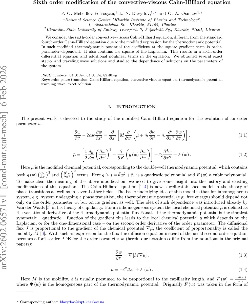
We consider the sixth-order convective-viscous Cahn-Hilliard equation, different from the standard fourth-order Cahn-Hilliard equation due to the modified expression for the thermodynamic potential. In such modified thermodynamic potential the coefficient at the square gradient term is order-parameter-dependent. It also contains the square of the Laplacian. This results in a sixth-order differential equation and additional nonlinear terms in the equation. We obtained several exact static- and traveling wave solutions and studied the dependence of solutions on the parameters of the system.

💡 Research Summary

The authors introduce a sixth‑order modification of the classical Cahn‑Hilliard (CH) equation by adding two higher‑order contributions to the free‑energy functional: a gradient‑coefficient that depends on the order parameter, g(w)=θw²+ε₁, and a square‑Laplacian term (Δw)² with coefficient ε₂. After a variational derivative, the chemical potential μ contains both a fourth‑order spatial derivative (ε₂∂⁴w) and nonlinear gradient terms. The resulting governing equation (1.1)‑(1.2) therefore becomes a sixth‑order partial differential equation (PDE) that also includes a convective term (−2ᾱw∂w/∂x′) and two viscous terms proportional to ∂w/∂t′ and ∂²∂x′²∂w/∂t′.

To analyse the model, the authors nondimensionalise the variables (w→u, x→x, t→t) using natural scales X=√ε₁ and T=ε₁M, which introduces dimensionless parameters α, η₁, η₂, θ, ε, ρ and the rescaled roots a₁<a₂<a₃ of the cubic bulk potential. In a travelling‑wave frame z=x−vt the PDE reduces to a fourth‑order ordinary differential equation (ODE) for u(z).

A key step is the Ansatz
u′(z)=κ(u−u₁)(u−u₂)=κ(u²−pu+q), p=u₁+u₂, q=u₁u₂,
which allows all higher derivatives to be expressed as polynomials in u. Substituting this Ansatz into the ODE and integrating once yields algebraic relations that must hold for the polynomial coefficients on both sides of the equation. This procedure leads to two fundamental constraints:

1. κ² = θ/(8ε) (Equation 2.22), which fixes the width of the wave in terms of the gradient‑coefficient θ and the higher‑order stiffness ε.
2. p(5θ+12η₂ακ)=0 (Equation 2.23), which splits the analysis into two distinct cases.

Static (p=0) case
When p=0, the solution is symmetric (u₁=−u₂) and the travelling speed v vanishes. The viscous coefficients η₁ and η₂ drop out of the static balance, and the remaining algebraic conditions (2.28)–(2.32) impose:
– a symmetry of the bulk potential (a₁+a₂+1=0),
– a positivity condition 4ερ>θ ensuring real wave amplitudes,
– a relation between the mobility‑scaled viscosity and the wave amplitude (ακ+u₂²=1 when the potential is symmetric).
The exact static profile is a hyperbolic tangent kink:
u(x)=−u₂ tanh(κu₂ x).

Traveling‑wave (p≠0) case
When p≠0, the convective term is active and the wave moves with speed v=−αp. The condition (3.1) forces α, κ and η₂ to satisfy ακη₂=−5θ/12, meaning that κ and α must have opposite signs because η₂>0. Further algebraic constraints (3.4)–(3.6) involve the ratio λ=η₁/η₂ and the bulk‑potential parameters (ρ, θ, a₁, a₂). Solving these yields a permissible interval for λ:

\