Regret of $H_\infty$ Preview Controllers

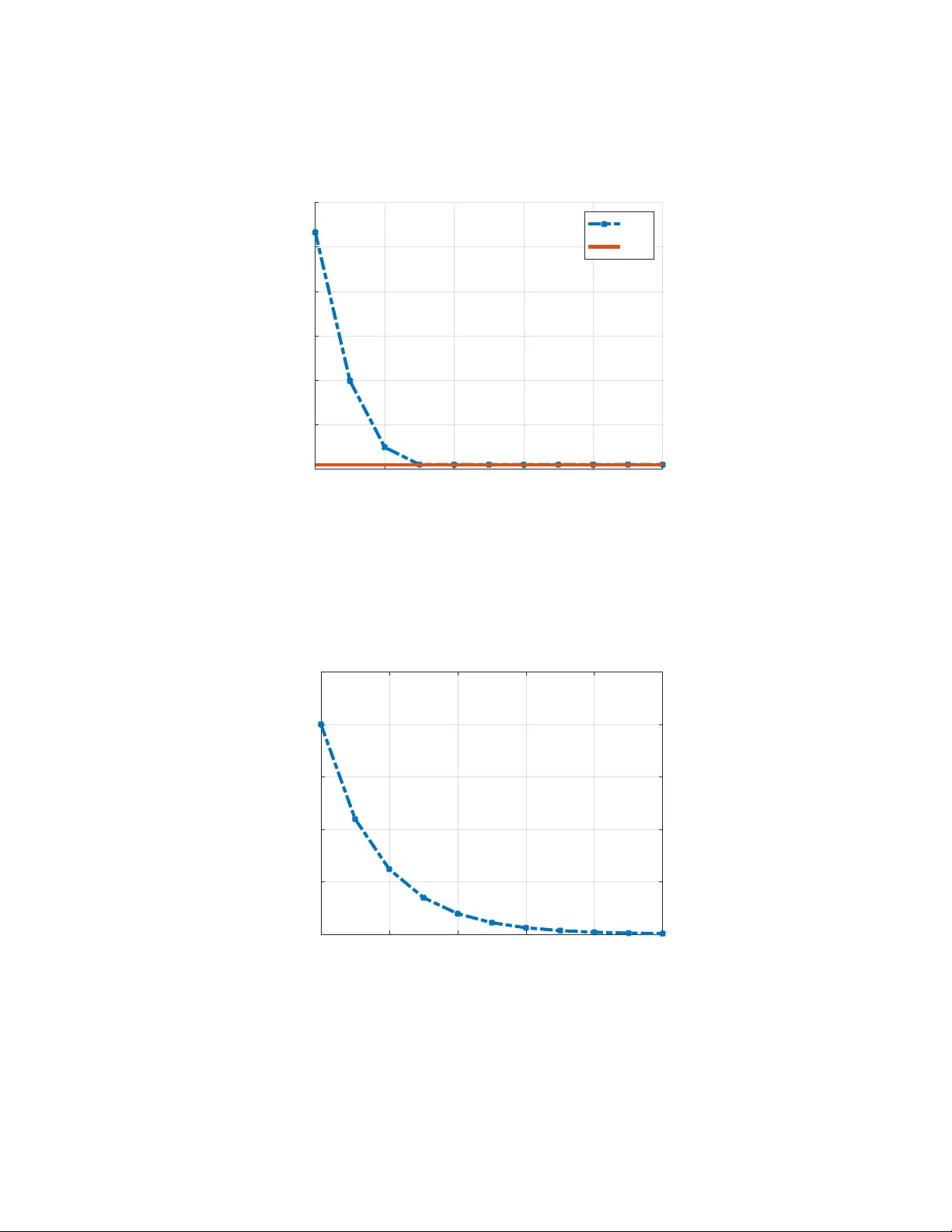
Regr et of H ∞ Pr eview Contr ollers Jietian Liu 1 and Peter Seiler 1 Abstract This paper studies previe w control in both the H ∞ and regret-optimal settings. The plant is modeled as a discrete-time, linear time-in v ariant system subject to external disturbances. The performance baseline is the optimal non-causal controller that has full kno wledge of the disturbance sequence. W e first re view the construction of the H ∞ previe w controller with p -steps of disturbance previe w . W e then show that the closed-loop H ∞ performance of this previe w controller con verges as p → ∞ to the performance of the optimal non-causal controller . Furthermore, we prov e that the optimal regret of the pre vie w controller con ver ges to zero. These results demonstrate that increasing pre view length allo ws controllers to asymptotically achiev e non- causal performance in both the H ∞ and regret frameworks. A numerical example illustrates the theoretical results. I . I N T RO D U C T I O N This paper considers pre vie w control in both the H ∞ and regret-optimal settings for discrete-time, linear time-in v ariant (L TI) systems subject to external disturbances. The classical H ∞ formulations [1], [2] ev aluate performance by minimizing the worst case of closed-loop gain from disturbance to error . These approaches provide powerful worst-case guarantees but do not explicitly account for the advantage of previe w information, nor do they compare performance against more informativ e non-causal benchmarks. Previe w control arises in applications where sensors provide advance measurements of external disturbances. For example, wind turbines equipped with LID AR sensors can measure the incoming wind field to improve po wer capture and reduce structural loads [3], [4], [5], while forward-looking sensors in acti ve vehicle suspensions provide previe w of the upcoming road profile [6], [7], [8], [9], [10], [11]. In these settings, future disturbances cannot be eliminated, but their effects can be anticipated and mitigated. This motiv ates robust previe w formulations, such as H ∞ previe w control, which exploit finite previe w information while providing worst-case performance guarantees under uncertainty . An alternativ e is regret-optimal control, which measures the performance of a causal controller relative to a baseline controller with greater information or capability . Regret is defined as the performance difference between the closed-loop cost of the causal controller and that of the baseline controller . T ypical measures for this performance dif ference include additiv e regret and competitiv e ratio. Prior works hav e considered baselines such as the optimal non-causal controller with full disturbance previe w [12], [13], [14], [15], [16], [17], [18], [19], [20], [21], [22], [23], [24], [25], [24], [26], [27], [28], or the best static state-feedback law [29], [30], [31]. Recently , sev eral studies have extended regret-optimal control to uncertain settings under the umbrella of robust or distributionally robust regret control[32], [33], [34], [35], [36], [37], [38], [39], [40]. These formulations typically neglect the previe w information. Recent work on regret-based control has also considered finite disturbance pre view , for example in predictiv e or MPC-based framew orks [41], [42]. In these approaches, previe w information is incorporated through receding-horizon optimization over a finite window . In contrast, the previe w formulation considered in this paper is defined with respect to an infinite-horizon cost, with pre view appearing only as an information constraint. There is a large literature on finite previe w control for H ∞ formulation in both finite horizon and infinite horizon [43], [44], [45], [46], [47], [48], [49], [50], [51], [52], [53], [54], [55], [56], [57], [58], [59], [60], [61], [62], [63], [64]. A common approach in discrete-time is to construct an augmented system with a chain of delays to store the disturbance previe w information. This technique simplifies the previe w control design as the standard H ∞ solutions can be applied to this augmented model. In this paper, we study the interplay between H ∞ previe w control and regret-optimal control with previe w . W e first revisit the standard synthesis of p -step H ∞ previe w controllers using state augmentation. W e then establish two key con v ergence results: (i) the H ∞ previe w controller achiev es closed-loop performance that con ver ges to the non-causal H ∞ bound as the previe w horizon grows, and (ii) the optimal regret of the p -step previe w controller con ver ges to zero as p → ∞ . Thus, previe w controllers asymptotically match the performance of the optimal non-causal controller . Previe w controllers require additional sensors to provide the previe w measurements. The benefit is that the pre view controllers are L TI with a well-understood theory . In contrast, more recent regret-based controllers con ver ge to the optimal non-causal controller over time by typically relying on time-varying, online optimization. These regret-based controllers do not require additional previe w sensors but are time-v arying, in general, and hence less understood. 1 Jietian Liu and Peter Seiler are with the Department of Electrical Engineering and Computer Science, Univ ersity of Michigan, Emails: jietian@umich.edu and pseiler@umich.edu I I . P RO B L E M F O R M U L A T I O N Consider a discrete-time, linear time-inv ariant (L TI) plant P with the following state-space representation: x ( t + 1 ) = Ax ( t ) + B d d ( t ) + B u u ( t ) , (1) where x ( t ) ∈ R n x is the state, d ( t ) ∈ R n d is the disturbance, and u ( t ) ∈ R n u is the control input at time t , respectiv ely . W e consider controllers with access to state measurements and finite previe w of the disturbance d ( t ) . Specifically , the controller has the follo wing information at time t : i p ( t ) : = { x ( t ) , d ( t ) , . . . , d ( t + p ) } , (2) where p ≥ 0 denotes the number of previe w steps. The case p = 0 corresponds to no previe w and is known as full information [1], [2], while p → ∞ corresponds to complete knowledge of all future disturbances. The goal is to design a p -step previe w controller K p to stabilize the plant and ensure good performance as measured with a linear quadratic cost. In particular, the cost for a controller K p ev aluated on a specific disturbance d ∈ ℓ 2 with initial condition x ( 0 ) = 0 is defined as follows: J ( K p , d ) : = ∞ ∑ t = 0 x ( t ) ⊤ Qx ( t ) + u ( t ) ⊤ Ru ( t ) . (3) Additional technical assumptions on the cost and state matrices will be giv en below to ensure the optimal control problem is well-posed. W e will use the optimal non-causal controller, denoted K nc , as a baseline for comparison, following [12], [14], [15], [16], [17], [18]. The controller K nc depends directly on the state as well as the present and all future values of d . The controller K nc is optimal in the sense that it minimizes J ( K , d ) for each d ∈ ℓ 2 . A solution for the optimal non-causal controller is given by Theorem 11.2.1 of [65]. Related non-causal results (both finite and infinite horizon) are given in [12], [14], [15], [16], [17], [18] where the non-causal controller is used as a baseline for regret-based control design. W e focus on the infinite-horizon case where the non-causal controller has access to the following information at time t : i nc ( t ) : = { x ( t ) , d ( t ) , d ( t + 1 ) , . . . } . (4) The optimal non-causal controller for the infinite-horizon case can be constructed using the stabilizing solution X of a discrete-time algebraic Riccati equation (D ARE). Specifically , the D ARE associated with the data ( A , B , Q , R ) is defined as follows: 0 = X − A ⊤ X A − Q + A ⊤ X B ( R + B ⊤ X B ) − 1 B ⊤ X A . (5) The next theorem provides a state-space model of K nc . Theorem 1. Let ( A , B u , B d , Q , R ) be given and assume: (i) Q ⪰ 0 and R ≻ 0 , (ii) ( A , B u ) stabilizable, (iii) A is nonsingular , and (iv) ( A , Q ) has no uno bs ervable modes on the unit cir cle . Then: 1) Ther e is a unique stabilizing solution X ⪰ 0 to DARE (5) defined by ( A , B u , Q , R ) . 2) Define the gain K x : = ( R + B ⊤ u X B u ) − 1 B ⊤ u X A. Then ˜ A : = A − B u K x is Schur and nonsingular . 3) Define a non-causal contr oller K nc with inputs i nc ( t ) given in (4) and output u nc ( t ) by the following non-causal state-space model: v nc ( t ) = ˜ A ⊤ [ v nc ( t + 1 ) + X B d d ( t )] , v nc ( ∞ ) = 0 , u nc ( t ) = − K x x ( t ) − K v v nc ( t + 1 ) − K d d ( t ) , (6) wher e K v : = ( R + B ⊤ u X B u ) − 1 B ⊤ u , K d : = ( R + B ⊤ u X B u ) − 1 B ⊤ u X B d . Then J ( K nc , d ) ≤ J ( K , d ) for any stabilizing contr oller K and disturbance d ∈ ℓ 2 . The Riccati-based results in items (1) and (2) of Theorem 1 are classical and follow from standard discrete-time LQR theory; see, e.g., [65], [1], [66]. The specific statement of Theorem 1 follows as a special case of Lemma 1 and Theorem 1 in [67]. 1 The assumption that A is nonsingular ensures that the closed-loop matrix ˜ A is also nonsingular . Note that the non-causal controller (6) can be reformulated so that the control input u nc ( t ) is expressed directly in terms of i nc ( t ) as defined in (4). Unrav eling the non-causal dynamics and noting that K d = K v X B d yields: u nc ( t ) = − K x x ( t ) − K v ∞ ∑ j = t  ˜ A ⊤  j − t X B d d ( j ) (7) 1 The results in [67] include a cross term x ⊤ Su in the cost function. Theorem 1 in this paper follows immediately by setting S = 0. Finally , we define the performance of any p -step previe w controller K p relativ e to the baseline, non-causal controller K nc as follo ws: Definition 1. Let γ > 0 be given. A p-step pre view contr oller K p achie ves γ -r egr et relative to the optimal non-causal contr oller K nc if the closed-loop is stable and: J ( K p , d ) − J ( K nc , d ) < γ 2 ∥ d ∥ 2 2 ∀ d ∈ ℓ 2 , d  = 0 . (8) Let γ R , p denote the minimal γ -regret achiev ed with p steps of previe w . W e will show that γ R , p → 0 as p → ∞ . I I I . BAC K G R O U N D : H ∞ C O N T RO L W I T H P R E V I E W This section revie ws the p -step H ∞ previe w controller , which provides the basis for the con ver gence results in Section IV. The formulation follows directly from the standard full-information H ∞ synthesis [1], [2], [68], [69] applied to an augmented system that encodes finite disturbance previe w . A γ -suboptimal H ∞ controller with p -step previe w can be constructed by augmenting the state to include future distur- bances. Related previe w results in both finite- and infinite-horizon settings can be found in [43], [44], [45], [46], [47], [48], [49], [50], [51], [52]. The augmented state at time t is defined as ˆ x p ( t ) : =      x ( t ) d ( t ) . . . d ( t + p − 1 )      ∈ R n x + pn d . (9) The resulting augmented plant is: ˆ x p ( t + 1 ) = ˆ A p ˆ x p ( t ) + ˆ B d , p d ( t + p ) + ˆ B u , p u ( t ) , (10) where d ( t + p ) denotes the p -step ahead disturbance available through previe w at time t . The system matrices are: ˆ A p =          A B d 0 · · · 0 0 0 I . . . . . . . . . . . . . . . . . . 0 . . . . . . . . . . . . I 0 · · · · · · · · · 0          , ˆ B u , p =     B u 0 . . . 0     , ˆ B d , p =     0 . . . 0 I     . (11) The cost can be rewritten in terms of the augmented state: J ( K p , d ) = ∞ ∑ t = 0 ˆ x p ( t ) ⊤ ˆ Q p ˆ x p ( t ) + u ( t ) ⊤ Ru ( t ) , (12) where ˆ Q p : = blkdiag ( Q , 0 , . . . , 0 ) is the state cost matrix. Using the augmented state ˆ x p ( t ) in (9), the p -step pre vie w problem can be formulated as a full-information H ∞ control problem on the augmented dynamics (10), where the exogenous input is d ( t + p ) and the measured signal is ˆ x p ( t ) . Giv en γ > 0, a controller is said to be γ -suboptimal if it stabilizes the augmented closed loop and satisfies J ( K p , d ) < γ 2 ∥ d ∥ 2 2 ∀ d ∈ ℓ 2 , d  = 0 . (13) Theorem 2. Fix p ≥ 0 and let ( ˆ A p , ˆ B u , p , ˆ B d , p , ˆ Q p , R ) be the augmented data defined in (10) – (12) and satisfy conditions ( i ) − ( iv ) in Theorem 1. F or any γ > 0 , a γ -suboptimal p-step pr evie w controller exists if and only if there exists a symmetric matrix ˆ X p such that: 1) ˆ X p satisfies the D ARE defined by ( ˆ A p , ˆ B p , ˆ Q p , ˆ R ) wher e ˆ B p : = [ ˆ B u , p , ˆ B d , p ] and ˆ R : = diag ( R , − γ 2 I ) . 2) H : = R + ˆ B ⊤ u , p ˆ X p ˆ B u , p ≻ 0 . 3) ∆ p : = γ 2 I − ˆ B ⊤ d , p ˆ X p ˆ B d , p + ˆ B ⊤ d , p ˆ X p ˆ B u , p H − 1 ˆ B ⊤ u , p ˆ X p ˆ B d , p ≻ 0 Mor eover , when these conditions hold, one γ -suboptimal pr evie w policy is u ∞ , p ( t ) = − ˆ K x , p ˆ x p ( t ) − ˆ K d , p d ( t + p ) , (14) wher e ˆ K x , p = H − 1 ˆ B ⊤ u , p ˆ X p ˆ A p and ˆ K d , p = H − 1 ˆ B ⊤ u , p ˆ X p ˆ B d , p . Theorem 2 follows directly by applying Theorem 9.2 of [68] to the augmented plant (10) with generalized error e ( t ) = ˆ C p ˆ x p ( t ) + Du ( t ) , where ˆ C p : = h ˆ Q 1 / 2 p 0 i ⊤ and D : =  0 R 1 / 2  ⊤ . W ith this choice, J ( K p , d ) = ∥ e ∥ 2 2 and the closed-loop induced ℓ 2 gain from d to e is less than γ if and only if (13) holds. This policy can be further expressed directly in terms of the plant state x ( t ) and previe wed disturbances: u ∞ , p ( t ) = − ˜ K x x ( t ) − ˜ K d d ( t ) − ˜ K v p ∑ j = 1 ˆ X j p d ( t + j ) , (15) where ˜ K x = H − 1 B ⊤ u ˆ X 0 p A , (16) ˜ K d = H − 1 B ⊤ u ˆ X 0 p B d , (17) ˜ K v = H − 1 B ⊤ u . (18) Here, we block partition the first n x rows of ˆ X p as follo ws:  ˆ X 0 p , ˆ X 1 p , . . . , ˆ X p p  , (19) where ˆ X 0 p ∈ R n x × n x and ˆ X j p ∈ R n x × n d for each j = 1 , . . . , p . The minimal achiev able γ with p steps of pre view is denoted γ ∞ , p . Thus, u ∞ , p ( t ) uses the previe w information i p ( t ) in the same additiv e structure as the non-causal controller, but truncated to p steps. I V . M A I N R E S U L T S In this section, we first recall the H 2 p -step pre view controller from Theorem 3 of [70]. Theorem 3. Let ( A , B u , B d , Q , R ) be given and satisfy conditions ( i ) − ( iv ) in Theor em 1. W e also assume the disturbance is the independent and identically distributed (IID) noise: E [ d i ] = 0 and E [ d i d ⊤ j ] = δ i j I for i , j ∈ { 0 , 1 , . . . } , where δ i j = 1 if i = j and δ i j = 0 otherwise. Define a H 2 p-step pr e view contr oller K 2 , p with inputs i p ( t ) given in (2) and output u 2 , p ( t ) by the following update equations: u 2 , p ( t ) = − K x x ( t ) − K v t + p ∑ j = t  ˜ A ⊤  j − t X B d d ( j ) , (20) wher e K x : = ( R + B ⊤ u X B u ) − 1 B ⊤ u X A , K v : = ( R + B ⊤ u X B u ) − 1 B ⊤ u , and X is a unique stabilizing positive solution to DARE (5) defined by ( A , B u , Q , R ) . Then this contr oller K 2 , p stabilizes the plant and solves: min K p stabilizing E [ J ( K p , d ) | i p ( 0 )] . (21) Note that Theorem 3 assumes IID noise and optimizes the expected cost in a stochastic formulation. Howe ver , we show next that the cost of H 2 previe w controller with finite previe w p < ∞ conv erges, in the limit as p → ∞ , to the optimal non-causal controller for any fixed (deterministic) disturbance d ∈ ℓ 2 . This result relies on the structural properties of the non-causal controller established in Theorem 1, and extends our prior work [70] from the stochastic setting to deterministic disturbance sequences. Lemma 1. Let ( A , B u , B d , Q , R ) be given and satisfy conditions ( i ) − ( iv ) in Theorem 1. Then, for any d ∈ ℓ 2 , lim p → ∞ J ( K 2 , p , d ) = J ( K nc , d ) . (22) Mor eover , the con ver g ence is uniform in d in the following sense: F or all ε > 0 there exists p ∗ such that for all p ≥ p ∗ , J ( K 2 , p , d ) − J ( K nc , d ) ≤ ε ∥ d ∥ 2 2 . (23) The proof of this lemma is gi ven in the Appendix. Lemma 1 can be used to show that the H ∞ previe w controller also con v erges in cost to the optimal non-causal controller . The formal statement of this result is giv en in the next theorem. Theorem 4. Define γ nc as the H ∞ norm of the closed-loop using the non-causal controller fr om Theorem 1. This corresponds to the minimal γ such that J ( K nc , d ) < γ 2 ∥ d ∥ 2 2 for all nonzer o d ∈ ℓ 2 . Similarly , let γ ∞ , p denote the H ∞ norm of the closed-loop using the p-step pr evie w H ∞ optimal contr oller fr om Equation 15. Then lim p → ∞ γ ∞ , p = γ nc . (24) Pr oof. It follows from Lemma 1 that J ( K 2 , p , d ) ≤  γ 2 nc + ε  ∥ d ∥ 2 2 . T aking the supremum over all nonzero d ∈ ℓ 2 giv es: γ 2 2 , p : = sup d ∈ ℓ 2 , d  = 0 J ( K 2 , p , d ) ∥ d ∥ 2 2 ≤ γ 2 nc + ε . The H ∞ controller K ∞ , p minimizes the induced ℓ 2 norm among all p -previe w controllers, γ nc ≤ γ ∞ , p ≤ γ 2 , p ≤ q γ 2 nc + ε . For any ˆ ε > 0, one can choose p suf ficiently large so that p γ 2 nc + ε < γ nc + ˆ ε . By the squeeze theorem, this establishes the claim. Theorem 5. Let γ R , p denote the minimal r e gret level in Definition 1 achievable by a p-step pr evie w controller . Then lim p → ∞ γ R , p = 0 , (25) and for any ˆ ε > 0 , there exist p and a controller K R , p such that 0 ≤ J ( K R , p , d ) − J ( K nc , d ) < ˆ ε ∀ d ∈ ℓ 2 , d  = 0 . (26) Pr oof. From (23), for any ε > 0 there exists p ∗ such that sup d ∈ ℓ 2 , d  = 0 J ( K 2 , p , d ) − J ( K nc , d ) ∥ d ∥ 2 2 ≤ ε ∀ p ≥ p ∗ . Since one can always find a K R , p that minimizes regret over all p -previe w controllers, γ 2 R , p ≤ sup d ∈ ℓ 2 , d  = 0 J ( K 2 , p , d ) − J ( K nc , d ) ∥ d ∥ 2 2 ≤ ε . For each fixed d ∈ ℓ 2 and ˆ ε > 0, one can find a p such that 0 ≤ J ( K R , p , d ) − J ( K nc , d ) ≤ γ 2 R , p ∥ d ∥ 2 2 ≤ ε ∥ d ∥ 2 2 ≤ ˆ ε , which prov es both claims. V . E X A M P L E This section uses a simple example to demonstrate the performance of previe w controllers in both the H ∞ and regret settings. 2 Consider the L TI system x ( t + 1 ) = Ax ( t ) + B d d ( t ) + B u u ( t ) , (27) with the follo wing parameters: A =  3 1 − 1 − 2  , B d =  1 1  , B u =  3 − 1  . The quadratic cost parameters are: Q =  3 0 0 3  , R = 1. Three controllers are synthesized for this system: 1. H ∞ Previe w Controller: For each previe w horizon p , we compute the optimal H ∞ p -step previe w controller K ∞ , p . This controller is computed using the approach outlined in Section III. W e use bisection to minimize γ within a small tolerance of 10 − 10 . W e denote the minimal (nearly optimal) feasible performance as γ ∞ , p . 2. Non-Causal Controller: The optimal non-causal controller K nc is designed according to Theorem 1. W e let γ nc denote the closed-loop H ∞ performance achie ved by the optimal non-causal controller . 3. Regret Pre view Controller: Finally , we synthesize the regret-optimal p -step previe w controller K R , p . This controller is computed using the approach outlined in [67] and Section III. The non-causal controller is first computed as in Theorem 1. Then a spectral factorization is used to transform the previe w regret problem into an equiv alent H ∞ previe w formulation. Finally , the transformed problem is solved as an H ∞ previe w problem using the same synthesis approach as above. Bisection is again used to minimize γ to within a tolerance of 10 − 10 . The minimal (nearly optimal) feasible performance is denoted by γ R , p . 2 The code to reproduce all results is available at: https://github.com/jliu879/Regret- of- Hinf- Preview- Controllers . First, we consider the closed-loop performance obtained by the (nearly) optimal p -step previe w controller, K ∞ , p . Figure 1 shows γ ∞ , p versus the previe w length p (blue dashed curve). The performance of the optimal non-causal controller , K nc , is also shown (red solid). The performance of the previe w controller γ ∞ , p improv es monotonically with increasing p and approaches the non-causal bound γ nc . This illustrates our result in Theorem 4 that γ ∞ , p → γ nc as p → ∞ . Previe w information enables the controller to asymptotically match the H ∞ performance of the non-causal baseline. 0 2 4 6 8 10 Preview p 3 4 5 6 7 8 9 H 1 norm . 1 ,p . nc Fig. 1. Closed-loop H ∞ norm of the p -step preview controller versus preview length p . The closed-loop H ∞ norm with the optimal non-causal controller is also shown. Next, we analyze the regret performance of the additive regret controller K R , p relativ e to the non-causal baseline K nc . Figure 2 shows the optimal regret bound γ R , p as a function of previe w length p . The regret decreases rapidly as p increases. This illustrates the result stated in Theorem 5: γ R , p → 0 as p → ∞ . Hence, pre vie w information enables the controller to asymptotically match the performance of the non-causal baseline in terms of regret as well. 0 2 4 6 8 10 Preview p 0 2 4 6 8 10 . R,p Fig. 2. Optimal additiv e regret γ R , p versus preview length p . Finally , the regret bound is always lar ger than the excess H ∞ gap, i.e., γ R , p ≥ γ ∞ , p − γ nc . Specifically , the follo wing inequality holds for any stabilizing controller K p : sup ∥ d ∥ < 1 [ J ( K p , d ) − J ( K nc , d )] ≥ sup ∥ d ∥ < 1 J ( K p , d ) − sup ∥ ˆ d ∥ < 1 J ( K nc , ˆ d ) . Minimizing both sides over stabilizing controllers K p yields γ 2 R , p ≥ γ 2 ∞ , p − γ 2 nc . Since γ ∞ , p > γ nc > 0, it follows that γ 2 ∞ , p − γ 2 nc ≥ ( γ ∞ , p − γ nc ) 2 . As a result, γ R , p ≥ γ ∞ , p − γ nc can be shown. Therefore, the conv ergence of regret to zero (Figure 2) is slower than the con v ergence of the H ∞ norm (Figure 1). T ogether , these results highlight that increasing previe w length improves both H ∞ performance and regret guarantees, and that both metrics con ver ge to their non-causal limits as p → ∞ . V I . C O N C L U S I O N S This paper studied previe w control in the H ∞ and regret-optimal framew orks. W e showed that the p -step H ∞ previe w controller achie ves closed-loop performance that con verges to the non-causal bound as p → ∞ . W e also proved that the optimal regret of the previe w controller conv erges to zero. This demonstrates that previe w enables controllers to asymptotically match non-causal performance. A numerical example confirmed these results. Future work will establish additional con ver gence properties, including con v ergence of the H ∞ previe w controller to the non-causal controller . AC K N OW L E D G M E N T This material is based upon work supported by the National Science Foundation under Grant No. 2347026. Any opinions, findings, and conclusions or recommendations expressed in this material are those of the author(s) and do not necessarily reflect the vie ws of the National Science Foundation. R E F E R E N C E S [1] K. Zhou, J. Doyle, and K. Glover , Robust and Optimal Control . Prentice-Hall, 1996. [2] G. Dullerud and F . Paganini, A Course in Robust Control Theory: A Con vex Approach . Springer , 1999. [3] A. Ozdemir , P . Seiler, and G. Balas, “Design tradeoffs of wind turbine preview control, ” IEEE T ransactions on Control Systems T echnology , vol. 21, no. 4, pp. 1143–1154, 2013. [4] D. Schlipf, D. Schlipf, and M. K ¨ uhn, “Nonlinear model predictiv e control of wind turbines using LIDAR, ” W ind energy , vol. 16, no. 7, pp. 1107–1129, 2013. [5] A. Scholbrock, P . Fleming, D. Schlipf, A. Wright, K. Johnson, and N. W ang, “Lidar-enhanced wind turbine control: Past, present, and future, ” in American Contr ol Conference , 2016, pp. 1399–1406. [6] M. T omizuka, “Optimum linear preview control with application to vehicle suspension”—revisited, ” Journal of Dynamic Systems, Measurement, and Contr ol , vol. 98, no. 3, pp. 309–315, 09 1976. [7] A. Ha ´ c, “Optimal linear previe w control of active vehicle suspension, ” V ehicle System Dyn. , vol. 21, no. 1, pp. 167–195, 1992. [8] H.-S. Roh and Y . Park, “Stochastic optimal previe w control of an activ e vehicle suspension, ” J. of Sound and V ibration , vol. 220, no. 2, pp. 313–330, 1999. [9] N. Louam, D. A. Wilson, and R. S. Sharp, “Optimal control of a vehicle suspension incorporating the time delay between front and rear wheel inputs, ” V eh. Sys. Dyn. , vol. 17, no. 6, pp. 317–336, 1988. [10] T . Y oshimura, K. Edokoro, and N. Ananthanarayana, “ An activ e suspension model for rail/vehicle systems with preview and stochastic optimal control, ” J. of Sound and V ibration , vol. 166, no. 3, pp. 507–519, 1993. [11] J. Marzbanrad, G. Ahmadi, H. Zohoor, and Y . Hojjat, “Stochastic optimal previe w control of a vehicle suspension, ” Journal of Sound and V ibration , vol. 275, no. 3, pp. 973–990, 2004. [12] G. Goel and B. Hassibi, “Competitiv e control, ” IEEE T ransactions on Automatic Control , vol. 68, no. 9, pp. 5162–5173, 2022. [13] G. Goel and A. W ierman, “ An online algorithm for smoothed regression and LQR control, ” in The 22nd International Conference on Artificial Intelligence and Statistics . PMLR, 2019, pp. 2504–2513. [14] G. Goel and B. Hassibi, “The power of linear controllers in LQR control, ” in IEEE Conference on Decision and Control . IEEE, 2022, pp. 6652–6657. [15] ——, “Regret-optimal measurement-feedback control, ” in Learning for Dynamics and Contr ol . PMLR, 2021, pp. 1270–1280. [16] O. Sabag, G. Goel, S. Lale, and B. Hassibi, “Regret-optimal controller for the full-information problem, ” in American Contr ol Conference , 2021, pp. 4777–4782. [17] O. Sabag, S. Lale, and B. Hassibi, “Competitiv e-ratio and regret-optimal control with general weights, ” in IEEE Conference on Decision and Control , 2022, pp. 4859–4864. [18] G. Goel and B. Hassibi, “Regret-optimal estimation and control, ” IEEE T rans. on Automatic Contr ol , vol. 68, no. 5, pp. 3041–3053, 2023. [19] G. Goel, N. Agarwal, K. Singh, and E. Hazan, “Best of both worlds in online control: Competitiv e ratio and policy regret, ” in Proceedings of The 5th Annual Learning for Dynamics and Contr ol Conference , vol. 211, 2023, pp. 1345–1356. [20] G. Goel and B. Hassibi, “Measurement-feedback control with optimal data-dependent regret, ” arXiv preprint , 2022. [21] H. Zhou and V . Tzoumas, “Safe control of partially-observed linear time-v arying systems with minimal worst-case dynamic re gret, ” in IEEE Confer ence on Decision and Contr ol , 2023, pp. 8781–8787. [22] A. Didier , J. Sieber, and M. N. Zeilinger, “ A system level approach to regret optimal control, ” IEEE Contr ol Systems Letters , vol. 6, pp. 2792–2797, 2022. [23] A. Martin, L. Furieri, F . D ¨ orfler , J. L ygeros, and G. Ferrari-Trecate, “Safe control with minimal regret, ” in Pr oceedings of The 4th Annual Learning for Dynamics and Contr ol Conference , vol. 168. PMLR, 23–24 Jun 2022, pp. 726–738. [24] A. Martin, L. Furieri, F . D ¨ orfler , J. Lygeros, and G. Ferrari-Trecate, “Follo w the clairvoyant: an imitation learning approach to optimal control*, ” IF AC-P apersOnLine , vol. 56, no. 2, pp. 2589–2594, 2023, 22nd IF A C W orld Congress. [25] J.-S. Brouillon, F . D ¨ orfler , and G. F . Trecate, “Minimal regret state estimation of time-varying systems, ” IF AC-P apersOnLine , vol. 56, no. 2, pp. 2595–2600, 2023, 22nd IF AC W orld Congress. [26] D. Martinelli, A. Martin, G. Ferrari-T recate, and L. Furieri, “Closing the gap to quadratic in variance: A regret minimization approach to optimal distributed control, ” in European Control Conference , 2024, pp. 756–761. [27] H. Tsukamoto, J. Hajar , S.-J. Chung, and F . Y . Hadaegh, “Regret-optimal defense against stealthy adversaries: A system lev el approach, ” in IEEE Confer ence on Decision and Control , 2024, pp. 1941–1948. [28] A. Karapetyan, A. Iannelli, and J. L ygeros, “On the regret of H ∞ control, ” in IEEE Conference on Decision and Contr ol , 2022, pp. 6181–6186. [29] N. Agarwal, B. Bullins, E. Hazan, S. Kakade, and K. Singh, “Online control with adversarial disturbances, ” in International Conference on Machine Learning . PMLR, 2019, pp. 111–119. [30] E. Hazan, “Introduction to online con vex optimization, ” F oundations and T r ends® in Optimization , vol. 2, no. 3-4, pp. 157–325, 2016. [31] Y . Li, S. Das, J. Shamma, and N. Li, “Safe adaptive learning-based control for constrained linear quadratic regulators with regret guarantees, ” 2021. [Online]. A vailable: https://arxiv .org/abs/2111.00411 [32] T . Kargin, J. Hajar, V . Malik, and B. Hassibi, “W asserstein distributionally robust regret-optimal control over infinite-horizon, ” in Proc. of the 6th Annual Learning for Dynamics and Control Conference , ser . Proceedings of Machine Learning Research, vol. 242. PMLR, 15–17 Jul 2024, pp. 1688–1701. [33] ——, “Infinite-horizon distributionally robust regret-optimal control, ” in Pr oceedings of the 41st International Conference on Machine Learning , ser . Proceedings of Machine Learning Research, R. Salakhutdinov , Z. K olter , K. Heller, A. W eller, N. Oliv er , J. Scarlett, and F . Berkenkamp, Eds., vol. 235. PMLR, 21–27 Jul 2024, pp. 23 187–23 214. [34] J. Hajar, T . Kargin, and B. Hassibi, “W asserstein distributionally robust regret-optimal control under partial observability , ” in Allerton Conf. on Communication, Contr ol, and Computing , 2023, pp. 1–6. [35] F . A. T aha, S. Y an, and E. Bitar, “ A distributionally robust approach to regret optimal control using the wasserstein distance, ” in IEEE Conference on Decision and Contr ol , 2023, pp. 2768–2775. [36] S. Y an and C. W . Scherer, “Distributional robustness in output feedback regret-optimal control, ” IF AC-P apersOnLine , vol. 59, no. 16, pp. 104–109, 2025, iF AC Symposium on Robust Control Design. [37] Y . Cho and I. Y ang, “W asserstein distributionally robust regret minimization, ” IEEE Contr ol Systems Letters , vol. 8, pp. 820–825, 2024. [38] A. Agarwal and T . Zhang, “Minimax regret optimization for robust machine learning under distrib ution shift, ” in Proceedings of Thirty F ifth Conference on Learning Theory , P .-L. Loh and M. Raginsky , Eds., vol. 178, 02–05 Jul 2022, pp. 2704–2729. [39] E. Bitar, “Distributionally robust regret minimization, ” 2024. [Online]. A vailable: https://arxiv .org/abs/2412.15406 [40] L.-B. Fiechtner and J. Blanchet, “W asserstein distributionally robust regret optimization, ” 2025. [Online]. A v ailable: https://arxiv .org/abs/2504.10796 [41] R. Zhang, Y . Li, and N. Li, “On the regret analysis of online lqr control with predictions, ” in American Control Confer ence . IEEE, 2021, pp. 697–703. [42] Y . Lin, Y . Hu, H. Sun, G. Shi, G. Qu, and A. Wierman, “Perturbation-based regret analysis of predictive control in linear time varying systems, ” 2021. [Online]. A v ailable: https://arxiv .org/abs/2106.10497 [43] H. W ang, H. Zhang, and L. Xie, “Discrete-time H ∞ previe w control problem in finite horizon, ” Mathematical pr oblems in engineering , vol. 2014, no. 1, 2014. [44] A. Hazell and D. J. Limebeer , “ An efficient algorithm for discrete-time H ∞ previe w control, ” Automatica , vol. 44, no. 9, p. 2441–2448, 2008. [45] D. Liu and Y . Lan, “Design of zero-sum game-based H ∞ optimal previe w repetitive control systems with external disturbance and input delay , ” International journal of r obust and nonlinear control , vol. 34, no. 16, p. 11065–11085, 2024. [46] T . Katayama and T . Hirono, “Design of an optimal servomechanism with previe w action and its dual problem, ” International journal of control , vol. 45, no. 2, p. 407–420, 1987. [47] H. Katoh, “ H ∞ -optimal preview controller and its performance limit, ” IEEE T ransactions on Automatic Control , vol. 49, no. 11, pp. 2011–2017, 2004. [48] A. Kojima, “Generalized previe w and delayed H ∞ control: output feedback case. ” IEEE, 2005, p. 5770–5775. [49] ——, “ H ∞ controller design for previe w and delayed systems, ” IEEE transactions on automatic contr ol , vol. 60, no. 2, p. 404–419, 2015. [50] A. Kojima and S. Ishijima, “ H ∞ performance of preview control systems, ” Automatica , vol. 39, no. 4, p. 693–701, 2003. [51] ——, “ H ∞ previe w tracking in output feedback setting, ” Int. journal of r obust and nonlinear contr ol , vol. 14, no. 7, p. 627–641, 2004. [52] ——, “Formulas on preview and delayed H ∞ control, ” IEEE transactions on automatic contr ol , vol. 51, no. 12, pp. 1920–, 2006. [53] G. T admor and L. Mirkin, “ H ∞ control and estimation with previe w-part i: matrix are solutions in continuous time, ” IEEE T r ansactions on Automatic Contr ol , vol. 50, no. 1, pp. 19–28, 2005. [54] ——, “ H ∞ control and estimation with previe w-part ii: fixed-size are solutions in discrete time, ” IEEE T ransactions on Automatic Contr ol , vol. 50, no. 1, pp. 29–40, 2005. [55] M. Grimble, “ H ∞ fixed-lag smoothing filter for scalar systems, ” IEEE T rans. on Signal Pr ocessing , vol. 39, no. 9, pp. 1955–1963, 1991. [56] P . Bolzern, P . Colaneri, and G. De Nicolao, “On discrete-time H ∞ fixed-lag smoothing, ” IEEE Tr ansactions on Signal Pr ocessing , vol. 52, no. 1, pp. 132–141, 2004. [57] A. Kojima and S. Ishijima, “Robust controller design for delay systems in the gap-metric, ” IEEE T ransactions on Automatic Control , vol. 40, no. 2, pp. 370–374, 1995. [58] G. T admor, “Robust control in the gap: a state-space solution in the presence of a single input delay , ” IEEE T ransactions on Automatic Control , vol. 42, no. 9, pp. 1330–1335, 1997. [59] L. Mirkin, “On the H ∞ fixed-lag smoothing: how to exploit the information previe w , ” Automatica , vol. 39, no. 8, pp. 1495–1504, 2003. [60] L. Mirkin and G. T admor, “Fixed-lag smoothing as a constrained version of the fixed-interval case, ” in American Control Conference , vol. 5, 2004, pp. 4165–4170. [61] L. Mirkin and G. Meinsma, “When does the H ∞ fixed-lag smoothing performance saturates?” IF AC Proceedings V olumes , vol. 35, no. 1, pp. 121–124, 2002, 15th IF A C W orld Congress. [62] H. W ang, H. Zhang, and L. Xie, “ H ∞ control for discrete-time systems with multiple previe w channels, ” in Pr oceedings of the 32nd Chinese Contr ol Confer ence , 2013, pp. 2316–2321. [63] Z. Huanshui, W . Hongxia, and W . Xuan, “ H ∞ control for systems with two classes of disturbances, ” in Pr oceedings of the 31st Chinese Contr ol Confer ence , 2012, pp. 183–188. [64] H. W ang, H. Zhang, and L. Xie, “Theoretical interpretation for some relationships in H ∞ setting, ” in 2010 8th W orld Congr ess on Intelligent Contr ol and Automation , 2010, pp. 226–231. [65] B. Hassibi, A. H. Sayed, and T . Kailath, Indefinite-Quadratic Estimation and Contr ol: A Unified Aapproac h to H 2 and H ∞ Theories . SIAM, 1999. [66] S. Chan, G. Goodwin, and K. Sin, “Con vergence properties of the riccati difference equation in optimal filtering of nonstabilizable systems, ” IEEE T r ansactions on Automatic Control , vol. 29, no. 2, pp. 110–118, 1984. [67] J. Liu and P . Seiler, “Robust regret optimal control, ” Int. Journal of Robust and Nonlinear Control , vol. 34, no. 7, pp. 4532–4553, 2024. [68] A. Stoorvogel, The H-infinity Contr ol Pr oblem: A State Space Approac h . Elsevier , 1993. [69] M. Green and D. Limebeer, Linear Robust Control , ser . Dover Books on Electrical Engineering. Dover Publications, Incorporated, 2012. [Online]. A vailable: https://books.google.com/books?id=CI- DyLffA CcC [70] J. Liu, L. Lessard, and P . Seiler , “Stochastic LQR design with disturbance previe w , ” 2025. [Online]. A v ailable: https://arxiv .org/abs/2412.06662 A P P E N D I X Here we provide the detailed proof of Lemma 1. Pr oof. By Theorem 3 of [70], the resulting cost difference can be expressed as: J ( K 2 , p , d ) − J ( K nc , d ) = ∞ ∑ t = 0 n − 2 d ( t ) ⊤ B ⊤ d ∞ ∑ l = p + 1 ( ˜ A ⊤ ) l X B d d ( t + l ) | {z } l ( t ) (28) + 2 x ( t ) ⊤ ( ˜ A ⊤ ) p + 1 X B d d ( t + p ) | {z } m ( t ) + [ 2 K v t + p ∑ j = t  ˜ A ⊤  j − t X B d d ( j ) + K v ∞ ∑ j = t + p + 1  ˜ A ⊤  j − t X B d d ( j )] ⊤ H [ ∞ ∑ l = p + 1 ( ˜ A ⊤ ) l X B d d ( t + l )] | {z } q ( t ) o . Define the finite constants a : = ∥ B ⊤ d ∥ 2 → 2 ∥ X ∥ 2 → 2 ∥ B d ∥ 2 → 2 < ∞ , (29) b : = ∥ B ⊤ d ∥ 2 → 2 ∥ X ∥ 2 → 2 ∥ K ⊤ v ∥ 2 → 2 ∥ H ∥ 2 → 2 ∥ X ∥ 2 → 2 ∥ B d ∥ 2 → 2 < ∞ . (30) Using Cauchy–Schwarz, reindexing of sums, and the fact that x ( t ) is linear time-inv ariant conv olutions of { d ( j ) } , one can deriv e the following bounds: ∞ ∑ t = 0 | l ( t ) | ≤ 2 a ∞ ∑ l = p + 1 ∥ ( ˜ A ⊤ ) l ∥ 2 → 2 ∞ ∑ t = 0 ∥ d ( t ) ∥∥ d ( t + l ) ∥ ! ≤ 2 a ∞ ∑ l = p + 1 ∥ ( ˜ A ⊤ ) l ∥ 2 → 2 ! ∥ d ∥ 2 2 , ∞ ∑ t = 0 | m ( t ) | ≤ 2 a ∞ ∑ t = 0 t − 1 ∑ j = 0  ∥ ( ˜ A ⊤ ) t − j + p ∥ 2 → 2 ∥ d ( j ) ∥∥ d ( t + p ) ∥  ≤ 2 a ∞ ∑ j = 0 ∞ ∑ t = j + 1  ∥ ( ˜ A ⊤ ) t − j + p ∥ 2 → 2 ∥ d ( j ) ∥∥ d ( t + p ) ∥  ≤ |{z} l : = t − j + p 2 a ∞ ∑ l = p + 1 ∥ ( ˜ A ⊤ ) l ∥ 2 → 2 ! ∥ d ∥ 2 2 , ∞ ∑ t = 0 | q ( t ) | ≤ 2 b ∞ ∑ t = 0 ∞ ∑ j = t ∞ ∑ l = p + 1  ∥ ( ˜ A ⊤ ) j − t ∥ 2 → 2 ∥ ( ˜ A ⊤ ) l ∥ 2 → 2 ∥ d ( j ) ∥∥ d ( t + l ) ∥  ≤ |{z} k : = j − t 2 b ∞ ∑ k = 0 ∞ ∑ l = p + 1 ∥ ( ˜ A ⊤ ) k ∥ 2 → 2 ∥ ( ˜ A ⊤ ) l ∥ 2 → 2 ∞ ∑ t = 0 ∥ d ( t + k ) ∥∥ d ( t + l ) ∥ ! ≤ 2 b ∞ ∑ k = 0 ∥ ˜ A k ∥ 2 → 2 ! ∞ ∑ l = p + 1 ∥ ( ˜ A ⊤ ) l ∥ 2 → 2 ! ∥ d ∥ 2 2 . In the bounds for l ( t ) , m ( t ) , and q ( t ) , we interchange the order of summation with respect to the time indices t , j , and l . This is justified as follows. After taking absolute values and operator norms, all summands become nonnegati v e. Hence, by T onelli’ s theorem, the order of summation over the corresponding countable index sets can be exchanged. Moreov er , for any fixed integer l ≥ 0, the inner sums satisfy ∞ ∑ t = 0 ∥ d ( t ) ∥ ∥ d ( t + l ) ∥ ≤  ∞ ∑ t = 0 ∥ d ( t ) ∥ 2  1 / 2  ∞ ∑ t = 0 ∥ d ( t + l ) ∥ 2  1 / 2 ≤ ∥ d ∥ 2 2 , by the Cauchy–Schwarz inequality and the fact that ∑ ∞ t = 0 ∥ d ( t + l ) ∥ 2 ≤ ∥ d ∥ 2 2 . Since ˜ A is Schur , ∑ ∞ l = p + 1 ∥ ( ˜ A ⊤ ) l ∥ 2 → 2 < ∞ , which guarantees that all rearranged series are finite. T o obtain an explicit conv ergence rate, we inv oke Gelfand’ s formula. Since ˜ A is Schur , there exists α ∈ ( ρ ( ˜ A ) , 1 ) and an integer T such that ∥ ˜ A j ∥ 2 → 2 ≤ α j for all j ≥ T . Consequently , for p ≥ T , ∞ ∑ l = p + 1 ∥ ( ˜ A ⊤ ) l ∥ 2 → 2 ≤ α p + 1 1 − α and c : = ∞ ∑ k = 0 ∥ ˜ A k ∥ 2 → 2 < ∞ . Combining the three bounds yields 0 ≤ J ( K 2 , p , d ) − J ( K nc , d ) ≤ ( 4 a + 2 bc ) α p + 1 1 − α ∥ d ∥ 2 2 , (31) which v anishes as p → ∞ for each fixed d ∈ ℓ 2 . In fact, the conv er gence is uniform if we restrict to ∥ d ∥ 2 ≤ 1.