Stochastic LQR Design With Disturbance Preview

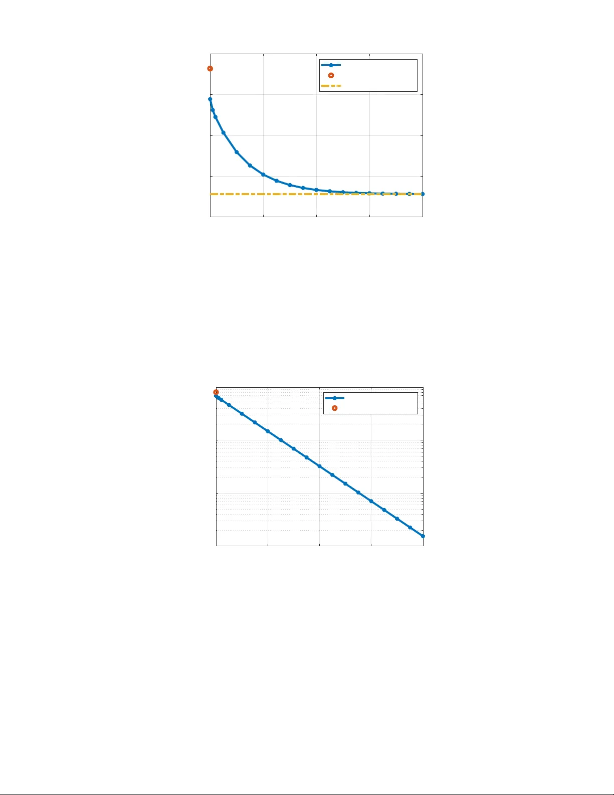
Stochastic LQR Design W ith Disturbance Pre vie w Jietian Liu Electrical Eng. and Computer Science University of Michigan jietian@umich.edu Laurent Lessard Mechanical and Industrial Eng . Northeastern University l.lessard@northeastern.edu Peter Seiler Electrical Eng. and Computer Science University of Michigan pseiler@umich.edu Abstract This paper considers the discrete-time, stochastic LQR problem with p steps of disturbance previe w information where p is finite. W e first deri ve the solution for this problem on a finite horizon with linear, time-varying dynamics and time-varying costs. Next, we derive the solution on the infinite horizon with linear, time-in variant dynamics and time-in variant costs. Our proofs rely on the well-known principle of optimality . W e provide an independent proof for the principle of optimality that relies only on nested information structure. Finally , we show that the finite previe w controller con verges to the optimal noncausal controller as the preview horizon p tends to infinity . W e also provide a simple example to illustrate both the finite and infinite horizon results. Index T erms Stochastic LQR, discrete time, disturbance pre vie w I . I N T RO D U C T I O N This paper considers control design for a discrete-time, stochastic Linear Quadratic Regulator (LQR) problem with finite previe w information of the disturbance. W e consider both the finite and infinite horizon problems. Our specific formulation is motiv ated by recent work on regret-based control [1], [2], [3], [4], [5], [6]. These regret-based formulations often use a controller with full knowledge of the disturbance as a baseline for performance. Then they show that a causal, time-v arying controller , updated with online optimization, can recover this baseline performance. W e show that the optimal stochastic LQR controller with finite previe w can also recover this baseline performance as pre vie w goes to infinity . Thus the performance of the noncausal controller can be recovered either via time-varying control with online optimization or using the stochastic LQR controller with an additional sensor to provide disturbance pre view . Recent work on regret-based control has also studied finite disturbance previe w , e.g., in predictive or MPC-based settings [7], [8]. These works typically consider bounded disturbances and deri ve non-asymptotic regret bounds. In contrast, we adopt a stochastic formulation with i.i.d. disturbances. Our previe w controller explicitly depends on the pre viewed disturbance realizations while optimizing the expected cost associated with post-previe w disturbances. Rather than deri ving regret bounds, we establish asymptotic con vergence of the finite-pre vie w LQR controller to the corresponding noncausal optimal controller as the previe w increases. There is a large literature on finite previe w control for stochastic LQR/LQG and its closely related H 2 formulation. These results exist in both continuous-time [9], [10], [11], [12], [13], [14], [15], [16], [17], [18], [19] and discrete-time [20], [21], [22], [23], [24], [25], [26], [27], [28], [29]. A common approach in discrete-time is to construct an augmented system with a chain of delays to store the disturbance previe w information. This technique simplifies the previe w control design as the standard LQR/LQG/ H 2 solutions can be applied to this augmented model [11], [20], [21], [13], [14], [23], [24], [25], [26], [16], [27], [17], [18], [28], [29]. The work in [15] is an exception as it use calculus of variations to directly derive necessary conditions for optimality . LQR/LQG/ H 2 with previe w is a reasonable formulation in applications where sensors provide previe w measurements of stochastic disturbances. For e xample, wind turbines must maximize power capture and reduce structural loads in the presence of wind speed fluctuations. LID ARs mounted on the turbine nacelle can measure the incoming wind field thus improving power capture and load reduction [30], [31], [32]. In this setting, the wind speed fluctuations are stochastic but can be measured with previe w . As a second example, active vehicle suspensions can be used to improve ride and handling qualities. Forw ard-looking radars measure the upcoming road profile. These measurements can be used for the activ e suspension control. Again, this setting can be modeled with a stochastic disturbance, i.e., the road profile, with previe w measurements [24], [15], [25], [26], [17], [18]. Our paper makes the follo wing contributions to this literature. First, we solve the stochastic LQR problems with finite disturbance previe w on both finite and infinite time horizons (SectionsV -A and V -B). In principle, these solutions follow from existing stochastic LQR results by using the state augmentation procedure. Howe ver , we provide an independent proof for the finite-horizon and infinite-horizon problems based on the principle of optimality . Moreov er, we provide a nov el proof for the principle of optimality in this setting (Section IV). Our proof only relies on the assumption of nested information and may be of independent interest. Finally , we compare the performance of the finite disturbance previe w controller against the optimal noncausal controller (Theorem 11.2.1 of [33]). The optimal noncausal controller has full knowledge of the future disturbance. W e sho w that the finite pre vie w controller con verges, in a certain sense, to the optimal noncausal controller as the pre view horizon tends to infinity (Section V -C). Finally , we illustrate the results with a simple example (Section VI). T wo of the most related works are [15] and [25]. Calculus of variations is used in [15] to derive a deterministic pre view control solution. The approach starts by deriving the optimal noncausal controller with full kno wledge of future disturbance, similar to that given in Theorem 11.2.1 of [33]. This optimal noncausal controller is then con verted to a finite-previe w controller by taking the expectation for una vailable future (post-previe w) information which is zero. In [25], an LQG problem is solved with a cost function that includes cross terms between the state and input. They address the finite pre vie w problem using an augmented state approach. The results in both [15] and [25] are similar to those contained in our paper . The key difference lies in the approach used to solve the problem. Specifically , our proof directly uses a version of the principle of optimality with nested information. This eliminates the need for state augmentation and hence our optimal controller is directly expressed with dynamics of the same order of the plant (not including augmented states). Moreov er , our finite horizon deriv ation can directly incorporate non-zero initial conditions. I I . N OTA T I O N Let R n and R n × m denote the sets of real n × 1 vectors and n × m matrices, respectively . The superscript ⊤ denote the matrix transpose. Moreover , if M ∈ R n × n then M ≻ 0 denotes that M is a symmetric positi ve definite matrix. Similarly , we use ⪰ , ≺ , and ⪯ for positi ve semidefinite, negati ve definite, and negati ve semidefinite matrices, respectiv ely . A matrix A ∈ R n × n is said to be Schur if the spectral radius is < 1 . W e also introduce random v ariables in the problem formulation and use E to denote the expectation. Finally , we denote the Kronecker delta δ ij where δ ij = 1 if i = j and δ ij = 0 otherwise. I I I . P RO B L E M F O R M U L A T I O N W e formulate the stochastic Linear Quadratic Regulator (LQR) problem with previe w information of the disturbance. The problem is stated on both finite and infinite horizons. Consider the discrete-time, linear time-varying (L TV) plant P with the following state-space representation: x t +1 = A t x t + B u,t u t + B w,t w t , (1) where x t ∈ R n x , u t ∈ R n u , and w t ∈ R n w are the state, input, and disturbance at time t , respectiv ely . The state matrices hav e compatible dimensions, e.g. A t ∈ R n x × n x , and are defined on a finite horizon t = 0 , 1 , . . . , T − 1 with T < ∞ . W e assume the disturbance is the independent and identically distributed (IID) noise: E [ w i ] = 0 and E [ w i w ⊤ j ] = δ ij I for i, j ∈ { 0 , 1 , . . . , T − 1 } . W e allow for the initial condition x 0 to be non-zero. The goal is to design a controller to reject the ef fect of the disturbance. W e assume the controller has measurements of the state and p steps of disturbance previe w where p ≥ 0 . Specifically , the controller has access to the following information at time t : i t : = { x 0 , . . . , x t , w 0 , . . . , w t + p } if t ≤ T − p − 1 i t : = { x 0 , . . . , x t , w 0 , . . . , w T − 1 } otherwise. (2) The av ailable information depends on the amount of previe w p ≥ 0 . Also note that the information i t contains some redundant information. Ho wev er, it is important that this information pattern is nested, i.e. i 0 ⊆ i 1 ⊆ · · · ⊆ i T − 1 . This allo ws the controller , in g e neral, to access past information as time goes on. This nesting structure is also used later in our formal proofs. W e allo w for controllers that can take random actions based on the av ailable information. Thus the controller policy at time t is specified by a probability density function ov er possible actions giv en the available information: K t ( u t , i t ) : = Prob ( u t | i t ) (3) This general formulation includes deterministic policies as a special case, which corresponds to functions of the form u t = k t ( i t ) . W e’ll denote the sequence of control policies by K : = { K 0 , . . . , K T − 1 } . The performance is ev aluated with a linear quadratic cost. In particular , the cost for a sequence of policies K ev aluated on a specific disturbance sequence w and initial condition x 0 is defined as follows: J T ( K, w, x 0 ) : = x ⊤ T Q T x T + T − 1 X t =0 x ⊤ t Q t x t + u ⊤ t R t u t , (4) where Q t ⪰ 0 for t = 0 , . . . , T and R t ≻ 0 for t = 0 , . . . , T − 1 . These matrices define the state and control costs. W e now state the finite-horizon (FH), stochastic LQR problem with pre vie w information. Problem 1 (FH Stochastic LQR With Previe w) . Consider the L TV plant (1) defined on t = 0 , . . . , T − 1 and cost function in (4) with Q t ⪰ 0 for t = 0 , . . . , T and R t ≻ 0 for t = 0 , . . . , T − 1 . Find a sequence of policies K : = { K 0 , . . . , K T − 1 } to solve: J ∗ T ,p ( i 0 ) : = min K E [ J T ( K, w, x 0 ) | i 0 ] . (5) The policy K t at time t uses information i t in (2) and includes p ≥ 0 steps of disturbance pre view . W e will also consider a similar problem on an infinite horizon. In this case, we will assume the plant P is linear , time-in variant (L TI): x t +1 = A x t + B u u t + B w w t , (6) where ( A, B ) are a stabilizable pair and A is nonsingular 1 . W e will also assume a sequence of (possibly random) control policies K : = { K 0 , K 1 , . . . } with p steps of disturbance previe w: i t : = { x 0 , . . . , x t , w 0 , . . . , w t + p } . (7) The cost function for a sequence of policies K e valuated on a specific disturbance w and initial condition x 0 is defined as the av erage per-step cost over the infinite horizon: J ∞ ( K, w, x 0 ) : = lim T →∞ 1 T T − 1 X t =0 x ⊤ t Qx t + u ⊤ t Ru t . (8) Here we assume Q ⪰ 0 , R ≻ 0 , and ( A, Q ) is detectable. The detectability assumption ensures that an y unstable modes in the plant will appear in the cost function. W e now state the infinite-horizon (IH), stochastic LQR problem with previe w information. W e restrict to policies that are stabilizing, i.e. the state remains uniformly bounded in both mean and second-moment. Problem 2 (IH Stochastic LQR W ith Previe w) . Consider the L TI plant (6) with A nonsingular, ( A, B ) stabilizable and cost function in (8) with Q ⪰ 0 , R ≻ 0 and ( A, Q ) detectable. Find a sequence of policies K : = { K 0 , K 1 . . . } to stabilize the plant and solve: J ∗ ∞ ,p ( i 0 ) : = min K stabilizing E [ J ∞ ( K, w, x 0 ) | i 0 ] . (9) The policy K t at time t uses information i t in (7) and includes p ≥ 0 steps of disturbance pre view . The IH cost could depend on the initial information i 0 for some policies, e.g. a policy could lead to unbounded trajectories and infinite cost for some initial conditions x 0 but not others. Howe ver , we will show in Section V -B that the optimal cost does not depend on the initial conditions, i.e. J ∗ ∞ ,p ( i 0 ) = J ∗ ∞ ,p . I V . P R I N C I P L E O F O P T I M A L I T Y Our solutions for the FH and IH problems with pre view will rely on the principle of optimality . This is a well known principle, e.g. see Section 2.2. of [35]. Here we will state a specific version that can be applied to the problems with disturbance previe w . W e state the principle of optimality for a more general, finite-horizon cost function: J ( K, i 0 ) : = E " g T ( x T ) + T − 1 X t =0 g t ( x t , u t )      i 0 # , (10) where the per-step cost functions g 0 , . . . , g T are gi ven. In this section we drop the subscripts in the cost function J to simplify the notation. The FH cost in the previous section is a special case where the g 0 , . . . , g T are quadratic functions. Moreov er , we will consider a more general information structure for i t . Specifically , we only assume that i t is nested, i.e. i t ⊆ i t +1 . The information structures in the previous section have this nested structure. The goal is to solve J ∗ ( i 0 ) = min K J ( K, i 0 ) . W e define the value function or optimal cost-to-go at time t as follo ws: V t ( i t ) : = min K t ,...,K T − 1 E   g T ( x T ) + T − 1 X j = t g j ( x j , u j )       i t   . (11) The v alue function at time t = 0 corresponds to the optimal cost: V 0 ( i 0 ) = J ∗ ( i 0 ) . The principle of optimality states that we can compute the value functions recursively , optimizing over one action at a time. 1 The solution to the infinite horizon problem (Section V -B) uses a related, discrete-time algebraic Riccati equation (DARE). There are technical issues in solving this DARE when A is singular . Our infinite horizon results can be extended to the case where A is singular using generalized solutions for the D ARE. See Section 21.3 and Remark 21.2 in [34] for details. Theorem 1 (Principle of Optimality) . Define the value function in (11) and assume the information is nested: i 0 ⊆ i 1 ⊆ · · · ⊆ i T − 1 . Then the value function satisfies the following backwards recursion starting from t = T : V T ( i T ) = E [ g T ( x T ) | i T ] , (12) V t ( i t ) = min u E [ g t ( x t , u t ) + V t +1 ( i t +1 ) | i t , u t = u ] (13) for t = 0 , . . . , T − 1 . Moreov er , the optimal cost J ∗ ( i 0 ) is achiev ed by a deterministic policy defined by selecting u t = k t ( i t ) at each t to minimize the value function in (13). Pr oof. Recall the value function defined in (11). No w define a recursive version as W T ( i T ) : = E [ g T ( x T ) | i T ] , W t ( i t ) : = min u E [ g t ( x t , u t ) + W t +1 ( i t +1 ) | i t , u t = u ] for t = 0 , . . . , T − 1 . W e will show , by induction, that W t = V t for all t . The base case W T = V T holds by definition. Next, make the induction assumption that W t +1 = V t +1 . W e will prov e that W t = V t holds as well. Consider the cost-to-go defined for any fixed set of policies { K t , . . . , K T − 1 } : V K t : T − 1 t ( i t ) : = E   g T ( x T ) + T − 1 X j = t g j ( x j , u j )       i t   . (14) W e can re-write this using the tower rule 2 V K t : T − 1 t ( i t ) = E [ g t ( x t , u t ) | i t ] + E   E   g T ( x T ) + T − 1 X j = t +1 g j ( x j , u j )       i t +1         i t   . (15) The tower rule applies due to the assumption of nested information, i t ⊆ i t +1 . The second term depends on the policies { K t +1 , . . . , K T − 1 } . W e can lower bound this term by the v alue function at time t + 1 . This gives: V K t : T − 1 t ( i t ) ≥ E [ g t ( x t , u t ) + V t +1 ( i t +1 ) | i t ] . (16) W e hav e W t +1 = V t +1 by the induction assumption. Next note that that the information i t is trivially a subset of the information { i t , u t } . Hence another application of the tower rule gives: V K t : T − 1 t ( i t ) ≥ E h E [ g t ( x t , u t ) + W t +1 ( i t +1 ) | i t , u t = u ]    i t i . (17) The right side depends on the polic y K t . As stated previously , this policy is specified by a probability density function K t ( u t , i t ) : = Prob ( u t | i t ) . W e can replace the outer expectation in (17) by an integral o ver all control actions: V K t : T − 1 t ( i t ) ≥ Z E [ g t ( x t , u t ) + W t +1 ( i t +1 ) | i t , u t = u ] K t ( u, i t ) du. (18) Finally , the right side is lo wer bounded by minimizing ov er the control input: V K t : T − 1 t ( i t ) ≥ min u E [ g t ( x t , u t ) + W t +1 ( i t +1 ) | i t , u t = u ] . (19) The right side is, by definition, W t ( i t ) . Thus we have sho wn that V K t : T − 1 t ( i t ) ≥ W t ( i t ) for an y set of policies { K t , . . . , K T − 1 } . This implies that the value function at time t satisfies V t ( i t ) ≥ W t ( i t ) . In fact, we can find a set of policies { K t , . . . , K T − 1 } that make V t ( i t ) = W t ( i t ) . For Equation 16, we have equality if we pick { K t +1 , . . . , K T − 1 } to be the optimal policies for the v alue function at t + 1 . For Equation 19, we achie ve equality by selecting a deterministic policy u t = k t ( i t ) with u t = arg min u E [ g t ( x t , u t ) + W t +1 ( i t +1 ) | i t , u t = u ] . The policy that achie ves J ∗ ( i 0 ) from will be deterministic if we use this choice for t = 0 to T − 1 . 2 W e have E  E [ x | y ]  = E [ x ] . More generally , whenever y ⊆ z , we have E [ E [ x | z ] | y ] = E [ x | y ] . See Theorem 9.1.5 in [36]. This is also known as the law of total expectation. Note that the proof only relies on the assumption of nested information. It does not use an y specific assumptions regarding the model / dynamics relating x t +1 and ( x t , u t ) (e.g., Markov assumption). It also does not rely on specific structure for the per-step cost functions g 0 , . . . , g T . That said, we will apply this version of the principle of optimality in the next section for the specific case with linear dynamics, quadratic cost functions, and nested information with disturbance previe w . V . M A I N R E S U LT S A. FH Stochastic LQR with Pre view This section presents the solution to the FH stochastic LQR problem with disturbance pre view (Problem 1). W e start with a standard technical lemma regarding a backwards Riccati iteration. Lemma 1. Let { A t } T − 1 t =0 ⊂ R n x × n x , { B u,t } T − 1 t =0 ⊂ R n x × n u , { Q t } T t =0 ⊂ R n x × n x , and { R t } T − 1 t =0 ⊂ R n u × n u be given. Assume Q t ⪰ 0 and R t ≻ 0 for each t . Define the following backwards Riccati iteration for t = 0 , . . . , T : P T : = Q T , (20) P t : = Q t + A ⊤ t P t +1 A t − A ⊤ t P t +1 B u,t H − 1 t B ⊤ u,t P t +1 A t , where H t : = R t + B ⊤ u,t P t +1 B u,t for t = 0 , . . . , T − 1 (21) Then P t ⪰ 0 for t = 0 , . . . , T . and H t ≻ 0 , for t = 0 , . . . , T − 1 . Hence H t is nonsingular for each t and the Riccati iteration is well defined. Pr oof. The proof is by induction. The base case is P T ⪰ 0 and H T − 1 ≻ 0 . This follows from the assumptions Q T ⪰ 0 and R T − 1 ≻ 0 . Next, make the induction assumption that P t +1 ⪰ 0 and H t ≻ 0 . W e will show that P t ⪰ 0 and H t − 1 ≻ 0 . Use the generalized matrix in version lemma (Fact 8.4.13 of [37]) to re write the Riccati iteration: P t = Q t + A ⊤ t P t +1  P t +1 + P t +1 B u,t R − 1 t B ⊤ u,t P t +1  † P t +1 A t , where † is the Moore-Penrose pseudo inv erse. Thus P t ⪰ 0 follo ws from P t +1 ⪰ 0 , Q t ⪰ 0 and R t ≻ 0 . Moreov er , P t ⪰ 0 combined with R t − 1 ≻ 0 imply H t − 1 ≻ 0 . The next theorem provides the solution to Problem 1. The proof is based on the principle of optimality (Theorem 1) and dynamic programming. Theorem 2. Consider the FH stochastic LQR with previe w including the assumptions stated in Problem 1. Define the following feedback gains using the solution of backwards Riccati iteration (20): K x,t : = H − 1 t B ⊤ u,t P t +1 A t , (22) K w,t : = H − 1 t B ⊤ u,t P t +1 B w,t , (23) K v ,t : = H − 1 t B ⊤ u,t . (24) The sequence of policies that achiev e J ∗ T ,p ( i 0 ) are deterministic, and hav e the form: u ∗ t = − K x,t x t − K w,t w t − K v ,t v t +1 , (25) where v t +1 depends on { w t +1 , . . . , w t + p } and is giv en by: v t +1 = t + p X j = t +1 h ˆ A ⊤ t +1 · · · ˆ A ⊤ j i P j +1 B w,j w j with ˆ A j : = A j − B u,j K x,j . (26) Equation 26 uses the con vention that w j = 0 when j ≥ T . Pr oof. The assumptions in Problem 1 are sufficient for Lemma 1 to hold. Hence the Riccati iteration and the feedback gains (22)-(24) are well-defined. Moreov er H t ≻ 0 for each t . Define the value function or optimal cost-to-go at time t for Problem 1 as follows: V t ( i t ) : = min K t ,...,K T − 1 E " x ⊤ T Q T x T + T − 1 X j = t x ⊤ j Q j x j + u ⊤ j R j u j      i t # . (27) The value function at time t = 0 corresponds to the optimal cost: V 0 ( i 0 ) = J ∗ T ,p ( i 0 ) . The value functions can be computed recursiv ely by the principle of optimality (Theorem 1): V T ( i T ) = E [ x ⊤ T Q T x T | i T ] V t ( i t ) = min u E h x ⊤ t Q t x t + u ⊤ t R t u t + V t +1 ( i t +1 )    i t , u t = u i for t = 0 , . . . , T − 1 . (28) W e will show that the v alue functions hav e the form: V t ( i t ) = x ⊤ t P t x t + 2¯ v ⊤ t x t + q t for t = 0 , . . . , T − 1 , (29) where { P t } T k =0 satisfy the backwards Riccati recursion (20), q t depend on { w t , . . . , w t + p } , and ¯ v t is giv en by: ¯ v t : = t + p X j = t h ˆ A ⊤ t · · · ˆ A ⊤ j i P j +1 B w,j w j . (30) Equation 30 again uses the con vention that w j = 0 if j ≥ T . 3 W e will show that (29) holds by induction. The base case at t = T corresponds to P T = Q T , ¯ v T = 0 , and q T = 0 . Next make the induction assumption that the v alue function at time t + 1 has the given form: V t +1 ( i t +1 ) = x ⊤ t +1 P t +1 x t +1 + 2¯ v ⊤ t +1 x t +1 + q t +1 . (31) W e will prov e that the v alue function at time t has the similar form given in (29). Substitute (31) into the value function recursion (28) and use the L TV dynamics (1) to replace x t +1 . This yields: V t ( i t ) = min u E [ x ⊤ t Q t x t + u ⊤ t R t u t + ( A t x t + B u,t u t + B w,t w t ) ⊤ P k +1 ( A t x t + B u,t u t + B w,t w t ) +2 ¯ v ⊤ t +1 ( A t x t + B u,t u t + B w,t w t ) + q t +1 | i t , u t = u ] . (32) Note that the quadratic term in this minimization is u ⊤ t H t u t where H t ≻ 0 . Thus the minimization has a unique minima because the objectiv e is a strictly conv ex function. T ake the gradient respect to u to find the optimal input: u ∗ t = E [ − K x,t x t − K w,t w t − K v ,t ¯ v t +1 | i t ] . (33) where the gains are defined in (22)-(24). Note that ( x t , w t ) are contained in i t so E [ x t | i t ] = x t and E [ w t | i t ] = w t . Moreover , the induction assumption giv es: ¯ v t +1 = t + p +1 X j = t +1 h ˆ A ⊤ t +1 · · · ˆ A ⊤ j i P j +1 B w,j w j . (34) Thus E [ ¯ v t +1 | i t ] = v t +1 and the optimal input in (33) simplifies to the expression in (25). Next, substitute u ∗ t back in to the cost-to-go function (32). After some simplification, the v alue function at time t has the form gi ven in (29) with P t giv en by the backwards Riccati recursion (20) and ¯ v t giv en by (30). Moreover , q t depends on { w t , . . . , w t + p } and can be simplified to: q t = − ( K w,t w t + K v ,t v t +1 ) ⊤ H t ( K w,t w t + K v ,t v t +1 ) + w ⊤ t B ⊤ w,t ( P t +1 B w,t w t + 2 v t +1 ) + E [ q t +1 | i t ] . Hence the proof is complete by induction. The optimal cost, based on the proof, is J ∗ T ,p ( i 0 ) = x ⊤ 0 P 0 x 0 + 2¯ v ⊤ 0 x 0 + q 0 . (35) The first term depends only on the state initial condition x 0 . The second term depends on both the x 0 and the initial disturbance information { w 0 , ..., w p } . The third term also depends on the initial disturbance information but also includes the expected cost of the disturbances { w p +1 , ..., w T − 1 } . 3 Note that ¯ v t depends on { w t , . . . , w t + p } . This means that ¯ v t +1 depends on { w t +1 , . . . , w t + p +1 } . Howe ver , v t +1 defined in (26) depends on { w t +1 , . . . , w t + p } . Hence ¯ v t +1 and v t +1 differ by one term. B. IH Stochastic LQR with Pre view This section presents the solution to the IH stochastic LQR problem with disturbance previe w (Problem 2). W e start with a standard technical lemma regarding a discrete time algebraic Riccati equation (DARE). Lemma 2. Let A ∈ R n x × n x , B u ∈ R n x × n u , Q ∈ R n x × n x , and R ∈ R n u × n u be giv en. Assume: (i) Q ⪰ 0 and R ≻ 0 , (ii) ( A, B u ) stabilizable, (iii) A is nonsingular , and (iv) ( A, Q ) has no unobservable modes on the unit circle. Then there is a unique stabilizing solution P ⪰ 0 such that: 1) P satisfies the follo wing DARE: 0 = P − A ⊤ P A − Q + A ⊤ P B u H − 1 B ⊤ u P A, (36) where H : = R + B ⊤ u P B u ≻ 0 . 2) The gain K x : = H − 1 B ⊤ u P A is stabilizing, i.e. A − B u K x is a Schur matrix. Pr oof. Statements 1) and 2) follow from Corollary 21.13 and Theorem 21.7 of [34] (after aligning the notation). The next theorem constructs the IH stochastic LQR with pre view controller using the stabilizing solution of the D ARE. Theorem 3. Consider the IH stochastic LQR with previe w including the assumptions stated in Problem 2. Define the following feedback gains using the solution of D ARE (36): K x : = H − 1 B ⊤ u P A, (37) K w : = H − 1 B ⊤ u P B w , (38) K v : = H − 1 B ⊤ u . (39) The sequence of policies that achiev e J ∗ ∞ ,p ( i 0 ) are deterministic, and hav e the form: u ∗ t = − K x x t − K w w t − K v v t +1 , (40) where v t +1 depends on { w t +1 , . . . , w t + p } and is giv en by: v t +1 = t + p X j = t +1 h ˆ A ⊤ i j − t P B w w j with ˆ A : = A − B u K x . (41) Pr oof. Recall that the infinite horizon cost for any sequence of policies K : = { K 0 , K 1 , . . . } is given by J ∞ ( K, w, x 0 ) : = lim T →∞ 1 T T − 1 X t =0 g ( x t , u t ) , (42) where g ( x t , u t ) : = x ⊤ t Qx t + u ⊤ t Ru t is the per-step cost. The main part of the proof is to re-arrange the per-step cost into a form that in volves u t − u ∗ t . This will be used to show that u t = u ∗ t is the optimal input. First, substitute for Q using the D ARE (36) and re-arrange to express the per-step cost as follo ws: g ( x t , u t ) =( u t + K x x t ) ⊤ H ( u t + K x x t ) + x ⊤ t P x t − ( Ax t + B u u t ) ⊤ P ( Ax t + B u u t ) . Use the L TI dynamics (6) to replace Ax t + B u u t by x t +1 − B w w t . This yields g ( x t , u t ) = ( u t + K x x t ) ⊤ H ( u t + K x x t ) + ( x ⊤ t P x t − x ⊤ t +1 P x t +1 ) − w ⊤ t B ⊤ w P B w w t + 2 x ⊤ t +1 P B w w t . Next, use the definition of u ∗ t in (40) to replace K x x t with − u ∗ t − K w w t − K v v t +1 . The per-step cost is thus given by g ( x t , u t ) = ( u t − u ∗ t ) ⊤ H ( u t − u ∗ t ) + ( x ⊤ t P x t − x ⊤ t +1 P x t +1 ) + l t − w ⊤ t B ⊤ w P B w w t − ( K w w t + K v v t +1 ) ⊤ H ( K w w t + K v v t +1 ) , (43) where l t : = − 2( K w w t + K v v t +1 ) ⊤ H ( u t + K x x t ) + 2 x ⊤ t +1 P B w w t . W e now focus on simplifying the term l t . W e have, from (38) and (39), that H K w = B ⊤ u P B w and H K v = B ⊤ u . Hence l t simplifies to: l t : = − 2( P B w w t + v t +1 ) ⊤ B u ( u t + K x x t ) + 2 x ⊤ t +1 P B w w t . W e can replace B u ( u t + K x x t ) with x t +1 − ˆ Ax t − B w w t . Combining terms yields: l t : = 2( P B w w t + v t +1 ) ⊤ ( ˆ Ax t + B w w t ) − 2 x ⊤ t +1 v t +1 . Note that the previe w term v t +1 defined in (41) satisfies the following relation: ˆ A ⊤ ( P B w w t + v t +1 ) = v t + h ˆ A ⊤ i p +1 P B w w t + p . (44) W e can use this to finally simplify l t to: l t = 2 x ⊤ t v t + 2 x ⊤ t h ˆ A ⊤ i p +1 P B w w t + p + 2 w ⊤ t B ⊤ w P B w w t + 2 v ⊤ t +1 B w w t − 2 x ⊤ t +1 v t +1 . Substitute this expression for l t back into the per-step cost (43). Re-organizing terms gi ves: g ( x t , u t ) = ( u t − u ∗ t ) ⊤ H ( u t − u ∗ t ) (45a) − ( K w w t + K v v t +1 ) ⊤ H ( K w w t + K v v t +1 ) (45b) + ( x ⊤ t P x t − x ⊤ t +1 P x t +1 ) + 2( x ⊤ t v t − x ⊤ t +1 v t +1 ) (45c) + 2 x ⊤ t h ˆ A ⊤ i p +1 P B w w t + p (45d) + 2 v ⊤ t +1 B w w t (45e) + w ⊤ t B ⊤ w P B w w t . (45f) The terms (45c) form telescoping sums when inserted into the cost J ∞ ( K, w, x 0 ) . The telescoping sums contribute zero to the cost as T → ∞ since the policy is assumed to be stabilizing. The expectation of term (45e) is zero as v t +1 depends on { w t +1 , . . . , w t + p } and is independent of w t . The expectation of term (45d) is also zero as x t depends on information i t − 1 = { x 0 , . . . , x t − 1 , w 0 , . . . , w t + p − 1 } , which is independent of w t + p . Thus the cost for any stabilizing polic y simplifies to: J ∗ ∞ ,p ( i 0 ) = min K stabilizing E  lim T →∞ 1 T T − 1 X t =0 ( u t − u ∗ t ) ⊤ H ( u t − u ∗ t ) − ( K w w t + K v v t +1 ) ⊤ H ( K w w t + K v v t +1 ) + w ⊤ t B ⊤ w P B w w t    i 0  . (46) Only the first term depends on the plant input and H ≻ 0 . Thus J ∗ ∞ ,p ( i 0 ) is achiev ed by u t = u ∗ t . The optimal IH cost is obtained by substituting u t = u ∗ t into (46). This yields: J ∗ ∞ ,p ( i 0 ) = lim T →∞ 1 T E  T − 1 X t =0 w ⊤ t B ⊤ w P B w w t − ( K w w t + K v v t +1 ) ⊤ H ( K w w t + K v v t +1 )    i 0  . This can be simplified further using the definition of v t +1 in (41) combined with E [ w i w ⊤ j ] = δ ij I . This gi ves: J ∗ ∞ ,p = trace  P B w B ⊤ w  − trace   p X j =0 H K v ( ˆ A ⊤ ) j P B w B ⊤ w P ˆ A j K ⊤ v   . (47) Here we ha ve used K w = K v P B w to simplify the expression further . Note that the optimal IH cost does not depend on the initial condition, i.e. J ∗ ∞ ,p ( i 0 ) = J ∗ ∞ ,p . The first term in the optimal cost, trace [ P B w B ⊤ w ] , is the cost that would be achie ved using only state feedback. The second term gives the cost reduction obtained by using the current disturbance measurement and p steps of previe w . C. Relation to Optimal Noncausal Contr oller This section discusses the optimal noncausal controller with full knowledge of the (past, current and future) values of the disturbance. W e focus on the IH case where the controller has access to the following information at time t : i t : = { x 0 , . . . , x t , w 0 , w 1 , . . . } . (48) The disturbance is fully kno wn so we consider deterministic policies K : = { k 0 , k 1 , . . . } where u t = k t ( i t ) . Moreov er , we assume w ∈ ℓ 2 and the (deterministic) cost is: ∞ X t =0 x ⊤ t Qx t + u ⊤ t Ru t . (49) Here the cost is deterministic (in contrast to the expected costs defined previously). The next problem states the IH design with full previe w . Problem 3 (IH LQR W ith Full Previe w) . Consider the L TI plant (6) with A nonsingular, ( A, B ) stabilizable and cost function in (49) with Q ⪰ 0 , R ≻ 0 and ( A, Q ) detectable. Also assume w ∈ ℓ 2 . Find a sequence of deterministic policies K : = { k 0 , k 1 . . . } to stabilize the plant and solve: min K stabilizing ∞ X t =0 x ⊤ t Qx t + u ⊤ t Ru t . (50) The policy k t at time t uses information i t in (48) and includes full previe w of the disturbance. A solution for the optimal noncausal controller is gi ven in Theorem 11.2.1 of [33]. Related noncausal results (both FH and IH) are gi ven in [1], [2], [3], [4], [5] where the noncausal controller is used as a baseline for regret-based control design. The next result gives the IH noncausal controller in a form/notation that closely aligns with the finite previe w controller in Theorem 3. Theorem 4. Consider IH LQR with full pre view including the assumptions stated in Problem 3. Define the feedback gains ( K x , K w , K v ) in (37)-(39) using the solution of DARE (36). The sequence of policies that achie ve the minimum are deterministic and hav e the form: u nc t = − K x x t − K w w t − K v v nc t +1 , (51) where v nc t +1 depends on { w t +1 , w t +2 , . . . } and is given by the following anticausal dynamics: v nc t = ˆ A ⊤ ( v nc t +1 + P B w w t ) , v nc ∞ = 0 with ˆ A : = A − B u K x . (52) This result, as stated, is a special case of Theorem 1 in [38]. It was stated in [38] for a more general LQR cost including a cross term 2 x ⊤ t S w t . 4 Note that the full pre vie w design (Problem 3) was stated with a deterministic formulation while finite previe w design (Problem 2) was derived with stochastic formulation. Howe ver , we show next that the controller with finite previe w p < ∞ con ver ges, in the limit as p → ∞ , to the optimal noncausal controller for any fixed disturbance w ∈ ℓ 2 . Theorem 5. Let w ∈ ℓ 2 be any gi ven (deterministic) disturbance sequence. Then the optimal noncausal controller is giv en by u nc t in (51) where v nc t +1 can be expressed as: v nc t +1 = ∞ X j = t +1 h ˆ A ⊤ i j − t P B w w j (53) Moreov er , let u p t denote the optimal finite previe w controller given in (40) with p < ∞ steps of previe w . Then ∥ u nc t − u p t ∥ 2 → 0 uniformly in t as p → ∞ . Pr oof. W e will first verify that (53) holds. Specifically , we will show that v nc t +1 defined by (52) is equal to the follo wing signal: y t +1 = ∞ X j = t +1 h ˆ A ⊤ i j − t P B w w j (54) It can be verified, by direct substitution, that y t +1 satisfies the state-space recursion in (52). Moreover , y t +1 satisfies the boundary condition y ∞ = 0 because w ∈ ℓ 2 and ˆ A is a Schur matrix. 5 Thus y t +1 is the unique solution to the noncausal dynamics in (52) and hence (53) holds. Next, we sho w that ∥ u nc t − u p t ∥ 2 → 0 uniformly in t as p → ∞ . Let x nc t and x p t denote the response of the L TI system (6) with some initial condition x 0 and disturbance w ∈ ℓ 2 using the noncausal and p -step finite previe w controller, respectiv ely . The difference between the two commands is: u nc t − u p t = − K x ( x nc t − x p t ) − K v ( v nc t +1 − v p t +1 ) . (55) 4 The proof given in [38] was for signals defined for t from −∞ to + ∞ . Howev er , the optimal noncausal controller is the same for signals defined from t = 0 to ∞ . 5 W e can bound y t +1 by ∥ y t +1 ∥ 2 ≤ a · b t where a :=    P ∞ l =1 [ ˆ A ⊤ ] l P B w    2 → 2 and b t := max j ≥ t +1 ∥ w j ∥ 2 . W e have a < ∞ because ˆ A is a Schur matrix. Moreover , b t → 0 as t → ∞ because w ∈ ℓ 2 . Hence y t +1 → 0 as t → ∞ . Next, note that the states satisfy the follo wing recursion: x nc t +1 − x p t +1 = A ( x nc t − x p t ) + B u ( u nc t − u p t ) = ˆ A ( x nc t − x p t ) − B u K v ( v nc t +1 − v p t +1 ) , where we hav e used (55) to substitute for u nc t − u p t . Iterating from x nc 0 − x p 0 = 0 (since the initial conditions match) giv es: x nc t − x p t = − t X j =1 ˆ A t − j B u K v ( v nc j − v p j ) . Substitute this back into (55) to express the dif ference in the control commands as follows: u nc t − u p t = − K v ( v nc t +1 − v p t +1 ) + K x t X j =1 ˆ A t − j B u K v ( v nc j − v p j ) . (56) T o bound the right side, we use (53) to rewrite ( v nc t +1 − v p t +1 ) in terms of the disturbance: v nc t +1 − v p t +1 = ∞ X l = p +1 ( ˆ A ⊤ ) l P B w w l + t . (57) Thus, ∥ v nc t +1 − v p t +1 ∥ 2 ≤ a p · b for t ≥ 0 , where a p :=       ∞ X l = p +1 [ ˆ A ⊤ ] l P B w       2 → 2 and b := max j ∥ w j ∥ 2 . The assumption w ∈ ℓ 2 implies that b is finite. Moreov er , ˆ A is a Schur matrix and hence a p → 0 as p → ∞ . 6 Finally , use this bound and Equation 56 to bound the dif ference in control commands: ∥ u nc t − u p t ∥ 2 ≤ a p b   c 1 + c 2 · t − 1 X j =0 ∥ ˆ A j ∥ 2 → 2   , (58) where c 1 := ∥ K v ∥ 2 → 2 and c 2 := ∥ K x ∥ 2 → 2 · ∥ B u K v ∥ 2 → 2 are finite constants. W e can choose any α ∈ ( ρ ( ˆ A ) , 1) and ∃ T such that    ˆ A j    ≤ α j for all j ≥ T . This follows from Gelfand’ s formula (Corollary 5.6.14 in [39]). Therefore, the sum P ∞ j =0 ∥ ˆ A j ∥ 2 → 2 con verges to some finite number c 3 . Thus we can bound the difference in control commands as: ∥ u nc t − u p t ∥ 2 ≤ a p b ( c 1 + c 2 c 3 ) , (59) where b , c 1 , c 2 , and c 3 are all finite constants. Moreover a p → 0 as p → ∞ . This implies that ∥ u nc t − u p t ∥ 2 → 0 uniformly in t as p → ∞ . Finally , we can derive a related con vergence result for the costs achiev ed with finite previe w and full, noncausal previe w . The optimal noncausal controller depends on the specific (deterministic) disturbance sequence and assumes w ∈ ℓ 2 to ensure the cost (49) is bounded. Ho wev er, we can apply the noncausal controller to stochastic disturbances w that are drawn from the distribution of IID, zero mean, unit variance sequences. The expected per-step cost for the optimal noncausal controller is: J ∗ ∞ ,nc ( x 0 ) : = E [ J ∞ ( K nc , w , x 0 ) | x 0 ] , (60) where K nc is the optimal noncausal controller (51) for a specific sequence w . The expected per-step cost for the noncausal controller is a veraged o ver stochastic signals w . W e show below that it does not depend on the initial state, i.e. J ∗ ∞ ,nc ( x 0 ) = J ∗ ∞ ,nc . The next result is that the expected per-step cost with the optimal finite previe w controller conv erges to the cost achieved by the optimal noncausal controller . W e also give a simple expression to compute the optimal cost achieved by the noncausal controller . 6 The sum P ∞ l = p +1 [ ˆ A ⊤ ] l con ver ges to ( I − ˆ A ⊤ ) − 1 ( ˆ A ⊤ ) p +1 . Thus, a p ≤ ∥ ( I − ˆ A ⊤ ) − 1 ∥ 2 → 2 · ∥ ( ˆ A ⊤ ) p +1 ∥ 2 → 2 · ∥ P B w ∥ 2 → 2 . W e hav e ( ˆ A ⊤ ) p +1 → 0 as p → ∞ and hence a p → 0 . Theorem 6. Let w be an IID sequence with E [ w i ] = 0 and E [ w i w ⊤ j ] = δ ij I for i, j ∈ { 0 , 1 , . . . } . The expected per-step cost for the optimal noncausal controller is: J ∗ ∞ ,nc = trace  P B w B ⊤ w  − trace  H K v X K ⊤ v  . (61) where X is the solution to the following discrete-time L yapunov equation: ˆ A ⊤ X ˆ A − X + P B w B ⊤ w P = 0 (62) Moreov er , let J ∗ ∞ ,p denote the optimal expected per-step cost in (47) achie ved by the optimal IH controller with p < ∞ steps of previe w . Then J ∗ ∞ ,p → J ∗ ∞ ,nc as p → ∞ . Pr oof. The steps in the proof of Theorem 3 can be used to show that the noncausal cost is gi ven by: J ∗ ∞ ,nc = trace  P B w B ⊤ w  − trace   ∞ X j =0 H K v ( ˆ A ⊤ ) j P B w B ⊤ w P ˆ A j K ⊤ v   . (63) The infinite sum con verges because ˆ A is a Schur matrix by Lemma 2. Moreover , the difference between the optimal finite previe w and noncausal costs is: J ∗ ∞ ,p − J ∗ ∞ ,nc = trace   ∞ X j = p +1 H K v ( ˆ A ⊤ ) j P B w B ⊤ w P ˆ A j K ⊤ v   . (64) The conv ergence J ∗ ∞ ,p → J ∗ ∞ ,nc follows because ˆ A is a Schur matrix. Finally , define X := P ∞ j =0 ( ˆ A ⊤ ) j P B w B ⊤ w P ˆ A j . X is the solution of the discrete-time L yapunov equation (62) (See Section 21.1 in [34]). This yields the expression for the optimal cost in (61). A consequence of the pre vious results is that the optimal finite previe w cost con verges geometrically to the optimal noncausal cost as p → ∞ . This is formally stated next. Corollary 1. Let w be an IID sequence with E [ w i ] = 0 and E [ w i w ⊤ j ] = δ ij I for i, j ∈ { 0 , 1 , . . . } . The difference between the optimal finite previe w and noncausal costs is: J ∗ ∞ ,p − J ∗ ∞ ,nc = trace h Y ( ˆ A ⊤ ) p +1 X ( ˆ A ) p +1 i . (65) where Y : = K ⊤ v H K v ⪰ 0 . This difference is bounded by: λ min ( X 1 2 ) 2 λ min ( Y 1 2 ) 2 ∥ ˆ A p +1 ∥ 2 F ≤ J ∗ ∞ ,p − J ∗ ∞ ,nc ≤ ∥ X 1 2 ∥ 2 F ∥ Y 1 2 ∥ 2 F ∥ ˆ A p +1 ∥ 2 F . (66) Pr oof. The dif ference between the optimal finite pre vie w and noncausal costs is giv en in Equation 64. This expression can be rewritten as follows: J ∗ ∞ ,p − J ∗ ∞ ,nc = trace   Y ( ˆ A ⊤ ) p +1   ∞ X j =0 ( ˆ A ⊤ ) j P B w B ⊤ w P ˆ A j   ˆ A p +1   . The summation in parentheses is, by definition, equal to X and this yields Equation 65. Next, re write this expression in terms of the Frobenius norm: (65): J ∗ ∞ ,p − J ∗ ∞ ,nc =   X 1 / 2 ( ˆ A ) p +1 Y 1 / 2   2 F . W e obtain the upper bound in (66) using the submultiplicativ e property of the Frobenius norm: ∥ P Q ∥ F ≤ ∥ P ∥ F ∥ Q ∥ F for any two matrices P and Q of appropriate dimensions. W e obtain the lower bound in (66) using the following property: ∥ P Q ∥ F ≥ λ min ( P ) ∥ Q ∥ F where P ⪰ 0 and Q is any matrix of appropriate dimension. The spectral radius formula gives the asymptotic approximation lim k →∞ ∥ ˆ A k ∥ 1 k = ρ ( ˆ A ) . Thus the asymptotic bounds in (66) as p → ∞ are approximated by: c 1 ρ  ˆ A  2( p +1) ≲ J ∗ ∞ ,p − J ∗ ∞ ,nc ≲ c 2 ρ  ˆ A  2( p +1) (67) where c 1 := λ min ( X ) λ min ( Y ) and c 2 := trace ( X ) trace ( Y ) are constants independent of p . This implies that the finite previe w cost con verges to the noncausal cost geometrically with p . V I . E X A M P L E This section presents two numerical examples to illustrate the proposed stochastic LQR framework with disturbance previe w . The first e xample considers a linear time-in variant (L TI) system and is included in the journal v ersion of the paper to demonstrate the basic structure and properties of the finite-horizon and infinite-horizon solutions. The second e xample considers a linear time- varying (L TV) mass–spring–damper system with time-varying dynamics and cost parameters. This second example illustrates the applicability of the proposed approach to time-varying settings. A. Boeing 747 Consider a simplified L TI model for the longitudinal dynamics of a Boeing 747 linearized at one steady , le vel flight condition (Problem 17.6 in [40]): x t +1 = A x t + B u u t + w t (68) where the state matrices are: A =  0 . 99 0 . 03 − 0 . 02 − 0 . 32 0 . 01 0 . 47 4 . 7 0 0 . 02 − 0 . 06 0 . 4 0 0 . 01 − 0 . 04 0 . 72 0 . 99  and B u =  0 . 01 0 . 99 − 3 . 44 1 . 66 − 0 . 83 0 . 44 − 0 . 47 0 . 25  . W e consider the IH and FH stochastic LQR problems with constant cost matrices Q = I and R = I at each step. This example was used in prior work on competitive ratio [6] and additive regret [1], [2]. Figure 1 shows the performance achiev ed by the optimal FH controller on the horizon T = 100 for previe ws p = 5 and 20 (solid lines). A closed-loop simulation was performed with a random disturbance. The plot shows the per-step cost averaged from time 0 to time t versus the time t . This is compared against the performance of the optimal H 2 controller computed on the IH (dashed lines). This H 2 controller is computed using a system augmented with delays to account for the disturbance previe w as in [21], [9], [27], [25], [26], [23]. This full information H 2 controller is computed using h2syn in Matlab . The optimal FH controller and IH H 2 controller hav e similar performance for t ≤ 60 . In fact, the FH and IH gains are similar at the beginning of the simulation. Howe ver , the FH gains deviate significantly from the IH gains near the end of the horizon. The FH gains are optimal for the horizon and hence the FH controller yields improv ed performance (lower av erage cost) by the end of the horizon. 0 20 40 60 80 100 Time 0 5 10 15 Average LQR cost Finite Preview, p=5 Finite Preview, p=20 H2SYN, p=5 H2SYN, p=20 Figure 1. Comparison of average cost obtained by optimal FH controller and optimal H 2 controller computed via an augmented system. Figure 2 shows the optimal IH cost versus the previe w horizon p (blue solid). The cost achieved by the finite pre view controller is computed using the expression in Equation 47. The plot also sho ws the cost achieved by the Linear Quadratic Regulator (LQR) state feedback: u t = − K x x t where K x = H − 1 B ⊤ u P A is the same gain as used in the finite previe w controller . The LQR state feedback achiev es a cost equal to trace [ P B w B ⊤ w ] ≈ 33 . 2 (red circle). The full information controller u t = − K x x t − K w w t corresponds to the case of p = 0 . This impro ves on the LQR performance and reduces the cost to ≈ 29 . 4 . Adding disturbance pre view ( p > 1) further decreases the cost. In fact, the cost monotonically decreases with increasing previe w . Figure 2 also sho ws the performance of the optimal noncausal controller (Theorem 4) for comparison. The cost for the optimal noncausal controller depends on the specific disturbance input. The yellow dashed line in Figure 2 corresponds to the expected (average) cost of the noncausal controller assuming white noise disturbances. This was computed using the expression 0 20 40 60 80 Preview, p 15 20 25 30 35 IH Cost Finite Preview, J $ 1 ;p LQR Non-causal, J $ 1 ;nc Figure 2. Comparison of IH cost versus previe w horizon p . giv en in Theorem 6. The noncausal controller has full knowledge of the disturbance and yields the lowest possible cost of ≈ 17 . 8 . The performance of the finite previe w controller conv erges, as p → ∞ , to the performance of the optimal noncausal controller . This is expected based on the discussion in Section V -C. Finally , Figure 3 shows the optimal IH relative error of the cost for the finite previe w controller compared to the cost for the optimal noncausal controller . This is normalized by the noncausal cost and plotted on a logarithmic scale against the previe w horizon p (blue solid). The plot uses the same cost results as in Figure 2. The plot is linear on a log scale in agreement with the geometric con vergence gi ven in Corollary 1. The slope on the log scale should be approximately 2 log ρ ( A ) . as p → ∞ . 0 20 40 60 80 Preview, p 10 -3 10 -2 10 -1 10 0 IH Relative Error ( J $ 1 ;p ! J $ 1 ;nc ) =J $ 1 ;nc ( J lq r ! J $ 1 ;nc ) =J $ 1 ;nc Figure 3. Comparison of IH relative error on a log scale versus pre view horizon p . B. Mass-spring-damper Consider a time-varying mass–spring–damper system with fixed damping ratio ζ and time-v arying natural frequency ω n ( k ) . The system is modeled directly in discrete time as a second-order linear time-varying system x k +1 = A k x k + B k u k + E k w k , k = 0 , 1 , . . . , T − 1 , (69) where x k = [ q k ˙ q k ] ⊤ denotes the displacement and velocity . The time-varying system matrices are gi ven by A k =  1 T s − T s ω n ( k ) 2 1 − 2 T s ζ ω n ( k )  , B k = E k =  0 T s  . This model corresponds to an Euler discretization of an equiv alent continuous-time, mass-spring-damper system with sample time T s . The simulation uses T s = 0 . 02 s and ζ = 0 . 7 . Moreov er , the natural frequency is giv en by: w n ( k ) = 1 . 5 + 0 . 5 sin  2 π T s k 10  ; (70) Finally , the disturbance w k is modeled as i.i.d. Gaussian noise. W e consider a finite-horizon stochastic LQR problem with time-varying state costs. Specifically , the input cost is fixed as R k = 0 . 1 , while the state cost Q k is chosen as diag(10 , 1) in the first half of the horizon and diag(50 , 1) in the second half. This penalizes the displacement more heavily later in the horizon. W e compute the optimal finite-horizon pre vie w controller for sev eral previe w horizons p and ev aluate its performance using closed-loop simulations. Figure 4 shows the average per-step cost from step 0 to step k versus the step index k for previe w horizons p ∈ { 1 , 5 , 20 } . The performance of the optimal noncausal controller is also shown. As expected, increasing the pre view horizon leads to improv ed performance (lo wer average cost). In particular, the performance with p = 20 is already very close to that of the noncausal controller . The noncausal controller , which has access to full disturbance information, achiev es the lo west cost and serves as a benchmark. 0 200 400 600 800 1000 Step 2 4 6 8 10 12 14 Average LQR cost # 10 -3 Finite Preview, p=1 Finite Preview, p=5 Finite Preview, p=20 Noncausal Figure 4. Comparison of average cost obtained by optimal FH controller and optimal noncausal controller in L TV system. V I I . C O N C L U S I O N This paper presented solutions to the discrete-time, stochastic LQR problem with p steps of disturbance previe w information where p is finite. Solutions were presented for both the finite horizon and infinite horizon problems. Moreover , we provided a proof for the principle of optimality that relies only on the assumption of nested information structure. This is of independent interest. Finally , we compared our solutions to sev eral existing results for optimal control with previe w information. Future work will explore using our finite-previe w controller as a baseline for regret-based design. Additionally , we will consider extensions to cases where the dynamic models and cost matrices are time-v arying and only known with finite previe w , in contrast to the full future knowledge assumed in this paper . V I I I . A C K N O W L E D G M E N T S This material is based upon work supported by the National Science Foundation under Grant No. 2347026. Any opinions, findings, and conclusions or recommendations expressed in this material are those of the author(s) and do not necessarily reflect the views of the National Science Foundation. R E F E R E N C E S [1] O. Sabag, G. Goel, S. Lale, and B. Hassibi, “Regret-optimal controller for the full-information problem, ” in American Control Conference , 2021, pp. 4777–4782. [2] ——, “Regret-optimal full-information control, ” , 2021. [3] O. Sabag, S. Lale, and B. Hassibi, “Optimal competitive-ratio control, ” , 2022. [4] G. Goel and B. Hassibi, “Regret-optimal estimation and control, ” IEEE T ransactions on A utomatic Contr ol , vol. 68, no. 5, pp. 3041–3053, 2023. [5] ——, “The power of linear controllers in LQR control, ” in IEEE Conference on Decision and Contr ol . IEEE, 2022, pp. 6652–6657. [6] ——, “Competitiv e control, ” IEEE T ransactions on Automatic Contr ol , vol. 68, no. 9, pp. 5162–5173, 2022. [7] R. Zhang, Y . Li, and N. Li, “On the regret analysis of online lqr control with predictions, ” in 2021 American Contr ol Confer ence (ACC) . IEEE, 2021, pp. 697–703. [8] Y . Lin, Y . Hu, H. Sun, G. Shi, G. Qu, and A. Wierman, “Perturbation-based regret analysis of predictiv e control in linear time varying systems, ” 2021. [Online]. A vailable: https://arxi v .org/abs/2106.10497 [9] A. Moelja and G. Meinsma, “ H 2 control of previe w systems, ” Automatica , v ol. 42, no. 6, pp. 945–952, 2006. [10] G. Marro and E. Zattoni, “ H 2 -optimal rejection with previe w in the continuous-time domain, ” Automatica , vol. 41, no. 5, pp. 815–821, 2005. [11] C. Sentouh, B. Soualmi, J. Popieul, and S. Debernard, “The H 2 -optimal pre view controller for a shared lateral control, ” in International Confer ence on Intelligent T ransportation Systems , 2011, pp. 1452–1458. [12] M. T omizuka, “Optimal continuous finite previe w problem, ” IEEE T rans. on Automatic Contr ol , vol. 20, no. 3, pp. 362–365, 1975. [13] A. Kojima and S. Ishijima, “LQ preview synthesis: optimal control and worst case analysis, ” IEEE T ransactions on Automatic Contr ol , vol. 44, no. 2, pp. 352–357, 1999. [14] A. Lindquist, “On optimal stochastic control with smoothed information, ” Information Sciences , vol. 1, no. 1, pp. 55–85, 1968. [15] A. Ha ´ c, “Optimal linear previe w control of activ e vehicle suspension, ” V ehicle System Dynamics , vol. 21, no. 1, pp. 167–195, 1992. [16] H. Peng and M. T omizuka, “Optimal previe w control for vehicle lateral guidance, ” California P A TH, T ech. Rep. UCB-ITS-PRR-91-16, 1991. [17] T . Y oshimura, K. Edokoro, and N. Ananthanarayana, “ An active suspension model for rail/vehicle systems with previe w and stochastic optimal control, ” J. of Sound and V ibration , vol. 166, no. 3, pp. 507–519, 1993. [18] J. Marzbanrad, G. Ahmadi, H. Zohoor, and Y . Hojjat, “Stochastic optimal preview control of a v ehicle suspension, ” Journal of Sound and V ibration , vol. 275, no. 3, pp. 973–990, 2004. [19] K. Hashikura, R. Hotchi, A. K ojima, and T . Masuta, “On implementations of H 2 previe w output feedback law with application to LFC with load demand prediction, ” International Journal of Contr ol , vol. 93, no. 4, pp. 844–857, 2020. [20] A. Hazell and D. Limebeer, “ A framework for discrete-time H 2 previe w control, ” Journal of Dynamic Systems, Measur ement, and Contr ol , vol. 132, no. 3, p. 031005, 04 2010. [21] K. T ing, M. Mesbahi, E. Li vne, and K. A. Morgansen, “W ind tunnel study of pre view H 2 and H ∞ control for gust load alleviation for flexible aircraft, ” AIAA SciT ech , 2022. [22] E. Zattoni, “ H 2 -optimal decoupling with pre view: a dynamic feedforward solution based on factorization techniques, ” in American Contr ol Confer ence , 2006, pp. 316–320. [23] M. T omizuka and D. E. Whitney , “Optimal Discrete Finite Previe w Problems (Why and How Is Future Information Important?), ” Journal of Dynamic Systems, Meas., and Contr ol , vol. 97, no. 4, pp. 319–325, 12 1975. [24] M. T omizuka, “Optimum Linear Previe w Control With Application to V ehicle Suspension—Revisited, ” Journal of Dyn. Systems, Meas., and Control , vol. 98, no. 3, pp. 309–315, 09 1976. [25] H.-S. Roh and Y . Park, “Stochastic optimal previe w control of an acti ve vehicle suspension, ” J. of Sound and V ibration , vol. 220, no. 2, pp. 313–330, 1999. [26] N. Louam, D. A. W ilson, and R. S. Sharp, “Optimal control of a vehicle suspension incorporating the time delay between front and rear wheel inputs, ” V ehicle System Dynamics , vol. 17, no. 6, pp. 317–336, 1988. [27] S. Y im, “Design of a previe w controller for vehicle rollover prevention, ” IEEE Tr ansactions on V ehicular T echnology , vol. 60, no. 9, pp. 4217–4226, 2011. [28] M. T omizuka and D. Rosenthal, “On the Optimal Digital State V ector Feedback Controller With Integral and Previe w Actions, ” J ournal of Dynamic Systems, Meas., and Contr ol , vol. 101, no. 2, pp. 172–178, 06 1979. [29] M. T omizuka and D. Fung, “Design of Digital Feedforward/Pre view Controllers for Processes W ith Predetermined Feedback Controllers, ” Journal of Dynamic Systems, Meas., and Contr ol , vol. 102, no. 4, pp. 218–225, 12 1980. [30] A. Ozdemir , P . Seiler, and G. Balas, “Design tradeof fs of wind turbine previe w control, ” IEEE T ransactions on Control Systems T echnology , vol. 21, no. 4, pp. 1143–1154, 2013. [31] D. Schlipf, D. Schlipf, and M. K ¨ uhn, “Nonlinear model predictive control of wind turbines using lidar, ” W ind ener gy , vol. 16, no. 7, pp. 1107–1129, 2013. [32] A. Scholbrock, P . Fleming, D. Schlipf, A. Wright, K. Johnson, and N. W ang, “Lidar-enhanced wind turbine control: Past, present, and future, ” in American Contr ol Confer ence . IEEE, 2016, pp. 1399–1406. [33] B. Hassibi, A. Sayed, and T . Kailath, Indefinite-Quadratic estimation and contr ol: a unified appr oach to H 2 and H ∞ theories . SIAM, 1999. [34] K. Zhou, J. C. Doyle, and K. Glover , Robust and optimal contr ol . Prentice hall, 1996. [35] B. Anderson and J. Moore, Optimal contr ol: linear quadratic methods . Prentice-Hall, 1990. [36] K. Chung, A Course in Pr obability Theory . Academic Press, 2001. [37] D. Bernstein, Scalar , vector , and matrix mathematics: theory , facts, and formulas-revised and expanded edition . Princeton Univ . Press, 2018. [38] J. Liu and P . Seiler, “Robust regret optimal control, ” Int. Journal of Robust and Nonlinear Contr ol , vol. 34, no. 7, pp. 4532–4553, 2024. [39] R. Horn and C. Johnson, Matrix analysis . Cambridge university press, 2013. [40] S. Boyd and L. V andenberghe, Intr oduction to Applied Linear Algebra: V ectors, Matrices, and Least Squares . Cambridge Univ . Press, 2018.