Sampling-Free Privacy Accounting for Matrix Mechanisms under Random Allocation

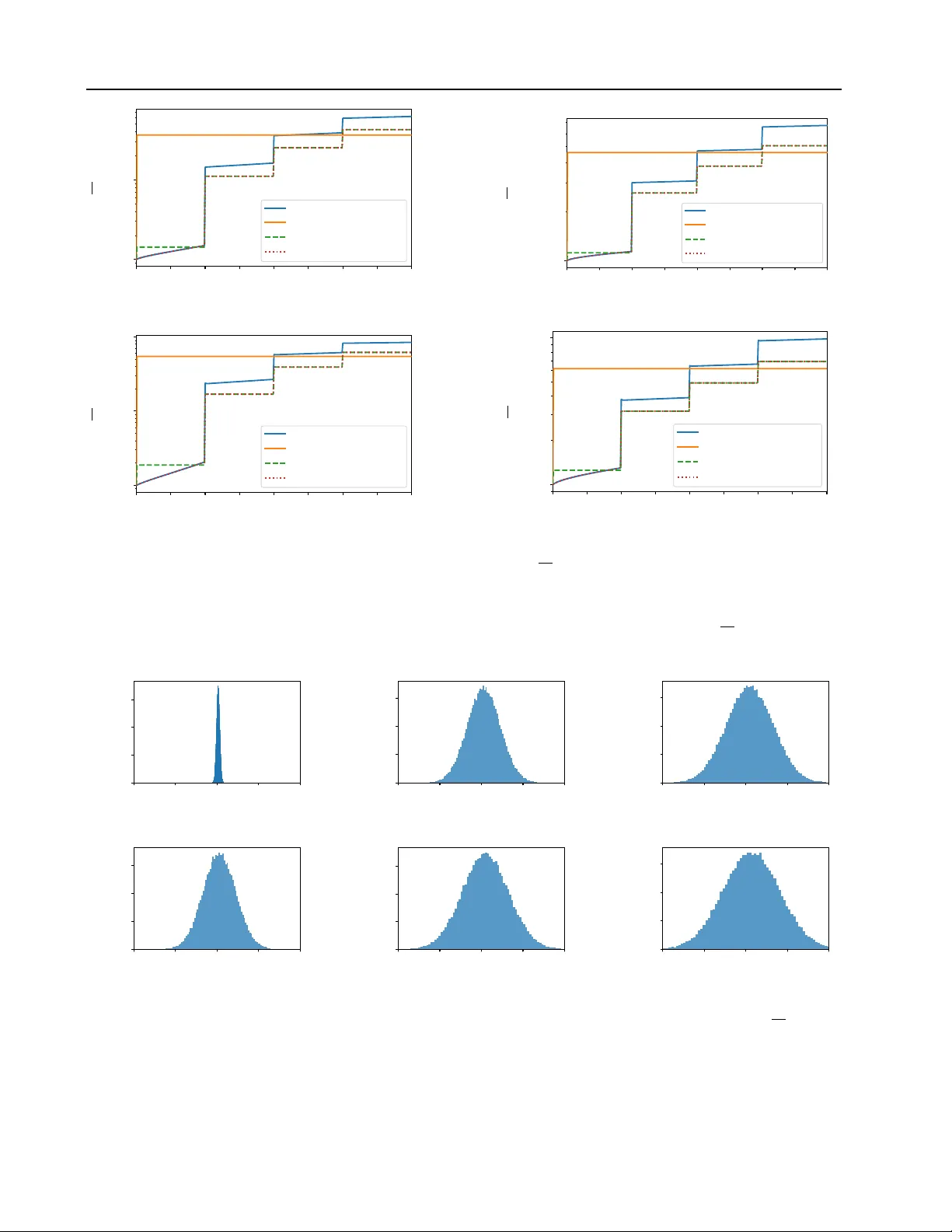
Sampling-Fr ee Priv acy Accounting f or Matrix Mechanisms under Random Allocation Jan Schuchardt 1 Nikita Kalinin 2 Abstract W e study pri v acy amplification for dif ferentially priv ate model training with matrix factorization under random allocation (also known as the balls- in-bins model). Recent work by Choquette-Choo et al. (2025) proposes a sampling-based Monte Carlo approach to compute amplification param- eters in this setting. Howe v er , their guarantees either only hold with some high probability or re- quire random abstention by the mechanism. Fur- thermore, the required number of samples for en- suring ( ε, δ ) -DP is in versely proportional to δ . In contrast, we dev elop sampling-free bounds based on R ´ enyi diver gence and conditional composi- tion. The former is facilitated by a dynamic pro- gramming formulation to efficiently compute the bounds. The latter complements it by offering stronger priv acy guarantees for small ε , where R ´ enyi diver gence bounds inherently lead to an ov er-approximation. Our framew ork applies to ar- bitrary banded and non-banded matrices. Through numerical comparisons, we demonstrate the ef- ficacy of our approach across a broad range of matrix mechanisms used in research and practice. 1. Introduction Differential pri vac y (DP) ( Dwork , 2006 ) offers one of the most well-established and mathematically rigorous defini- tions of pri vac y in statistical learning. In the context of deep learning, it is typically enforced via dif ferentially private stochastic gradient descent (DP-SGD) ( Abadi et al. , 2016 ). In DP-SGD, per-example gradients are clipped to bound the contribution of an y individual data point, and Gaussian noise is added to guarantee pri vacy . While the injected noise inevitably de grades model utility , this loss can be mitigated through priv acy amplification by subsampling ( Li et al. , 2012 ). Specifically , by randomly sampling a subset of the data at each iteration, we can achie ve the same pri vac y guar- antees with less additi ve noise. This improv ement arises 1 Machine Learning Research, Morgan Stanley 2 Institute of Sci- ence and T echnology Austri a. Correspondence to: Jan Schuchardt < jan.a.schuchardt@morganstanle y .com > . from the adversary’ s uncertainty about which examples are included in each batch, introducing additional randomness that strengthens the ov erall priv acy guarantees. Sev eral subsampling schemes have been studied in the con- text of dif ferentially priv ate training. One of the most com- monly used is Poisson subsampling ( Abadi et al. , 2016 ; Mironov , 2017 ; Kosk ela et al. , 2020 ; Zhu et al. , 2022 ), in which each data point is independently included in a batch with a fixed probability chosen to achieve a desired ex- pected batch size. Howe ver , this scheme poses practical challenges for implementation ( Lebeda et al. , 2025 ; Bel- tran et al. , 2024 ). In particular, for lar ge datasets and long training runs, two issues arise. First, drawing an indepen- dent random subset at e very iteration is often computation- ally infeasible. Second, subsampling can lead to unev en data cov erage, with a substantial fraction of examples (ap- proximately 1 /e ) not appearing within an epoch, and may increase the v ariance of gradients ( Feldman & Shenfeld , 2025 ). As a result, a common but problematic practice is to train on shuffled data while reporting pri vac y guarantees deriv ed for Poisson subsampling ( Lebeda et al. , 2025 ). A principled alternativ e that has emerged to address this issue is the “balls-in-bins” scheme ( Chua et al. , 2025 ; Choquette-Choo et al. , 2025 ), also known as balanced itera- tion subsampling ( Dong et al. , 2025 ) or as random alloca- tion ( Feldman & Shenfeld , 2025 ). This approach predefines batches for an entire epoch and reuses them throughout training, ensuring a fixed number of participations per data point. As a result, it mitigates both the per-iteration sam- pling ov erhead and the uneven within-epoch data co verage, while requiring a noise multiplier comparable to that of Poisson subsampling to attain the same priv acy guarantees. Beyond better subsampling schemes, another principled ap- proach to improv e upon the utility DP-SGD is to introduce correlated noise. The key idea is to add more noise at each iteration while carefully correlating it across steps so that the aggregate noise has lo wer variance than in standard DP- SGD, thereby improving model utility . The most common way to implement such noise correlations is through the ma- trix factorization mechanism ( Li et al. , 2015 ; Denisov et al. , 2022 ; Choquette-Choo et al. , 2023b ; a ), where Gaussian noise Z is correlated across iterations via the linear transfor - 1 Sampling-Free Pri vacy Accounting f or Matrix Mechanisms under Random Allocation mation C − 1 , i.e., sampling C − 1 Z , and then adding it to the gradients. Matrix factorization, howe ver , can be impractical at scale, motiv ating memory-ef ficient structured variants. Prior work proposes banded matrix f actorizations ( Kalinin & Lampert , 2024 ; McKenna , 2025 ), where the strategy matrix C is banded and T oeplitz; banded-in verse factor- izations ( Kalinin et al. , 2025 ), where C − 1 is banded; and hybrid constructions such as the Buffered Linear T oeplitz (BL T) matrix ( Dvijotham et al. , 2024 ; McMahan et al. , 2024 ). These designs enable correlated-noise mechanisms with substantially reduced memory requirements. Priv acy amplification by subsampling and noise correlation techniques can be combined. This has been demonstrated for banded matrix mechanisms under Poisson subsampling ( Choquette-Choo et al. , 2023a ; 2024 ), and more recently for general correlation matrices using balls-in-bins subsampling ( Choquette-Choo et al. , 2025 ). The latter , ho wever , relies on Monte Carlo estimation, which can require an intractably large number of samples in the high-priv acy regime and thus become computationally expensi ve. Moreover , it does not directly yield deterministic DP guarantees, but rather priv acy bounds that only hold with high probability . Motiv ated by the recent independent w orks of Feldman & Shenfeld ( 2025 ); Dong et al. ( 2025 ), who derived pri vacy bounds for DP-SGD under balls-in-bins batching without Monte Carlo sampling, we propose two procedures for com- puting amplification bounds for matrix mechanisms under this batching scheme. Our methods avoid Monte Carlo sam- pling entirely and instead compute the bounds explicitly , lev eraging R ´ enyi di vergence via dynamic programming as well as conditional composition while accounting for the inter-step correlations unique to matrix mechanisms. Contribution • W e introduce deterministic, R ´ enyi diver gence based and conditional composition based priv acy analyses (accountants) for subsampled matrix mechanisms. • For the special case of DP-SGD, we improv e the com- putational complexity of R ´ enyi accounting under the random allocation (balls-in-bins) batching scheme. 2. Background 2.1. Definitions of Differential Pri vacy Differ ential Privacy (DP) is a widely accepted framew ork for providing rigorous priv acy guarantees. W e recall its definition below: Definition 2.1 (Differential Pri vac y ( Dwork , 2006 )) . A ran- domized mechanism is said to provide ( ε, δ ) -differential priv acy under a neighboring relation ≃ if, for all datasets D ≃ D ′ , and for all measurable subsets S of the mecha- nism’ s output space: Pr[ M ( D ) ∈ S ] ≤ e ε · Pr[ M ( D ′ ) ∈ S ] + δ. (1) In the follo wing, we write M ( · | D ) for the distribution of random variable M ( D ) . W e further use an equiv alent definition of differential priv acy that is more con venient for pri vacy accounting, i.e., tracking priv acy o ver multiple applications of a mechanism. Lemma 2.2 (Proposition 2 from ( Barthe & Olmedo , 2013 )) . A mechanism pr ovides ( ε, δ ) -DP under ≃ if and only if, for all D ≃ D ′ , H e ε ( M ( · | D ) , M ( · | D ′ )) ≤ δ with hocke y- stick diver gence H γ ( P || Q ) = E x ∼ P  max  1 − γ d Q d P ( x ) , 0  . (2) While ( ε, δ ) -DP corresponds to a bound on the hock ey-stick div ergence for a single choice of γ = e ε , tight pri vacy accounting requires bounds for all choices of γ . In the following, we recall multiple equi valent ( Zhu et al. , 2022 ) characterizations of this privacy pr ofile that are immediately relev ant to our work, beginning with dominating pairs: Definition 2.3. W e say that the pair of distrib utions ( ˆ P , ˆ Q ) dominates ( P , Q ) , denoted by ( P , Q ) ≺ ( ˆ P , ˆ Q ) , if H γ ( P || Q ) ≤ H γ ( ˆ P , ˆ Q ) for all γ > 0 . Definition 2.4 ( Zhu et al. ( 2022 )) . W e say that ( ˆ P , ˆ Q ) are a dominating pair of mechanism M under neighboring rela- tion ≃ if ( M ( · | D ) , M ( · | D ′ )) ≺ ( ˆ P , ˆ Q ) for all D ≃ D ′ . Giv en a dominating pair ( P , Q ) , the problem of priv acy ac- counting reduces to quantifying the hockey-stick di ver gence H γ ( P || Q ) . Specifically , the div ergence does not directly depend on the (potentially high-dimensional) structure of ( P , Q ) b ut on their log-likelihood ratio, the “priv acy loss”: Definition 2.5. The priv acy loss random v ariable L P,Q of two distrib utions P , Q is log( d P d Q ( x )) with x ∼ P . From Equation ( 2 ) and γ d P d Q ( x ) = e log( γ ) − L P,Q , we see that the hockey-stick di vergence quantifies how much the priv acy loss random v ariable exceeds ε = log( γ ) (in ex- pectation). While the density of L P,Q fully determines the priv acy profile, it is often analytically more con venient to work with its moment-generating properties. Specifically , the priv acy loss distribution is uniquely characterized by its cumulant generating function ( Zhu et al. , 2022 ), which is proportional to the R ´ enyi di vergence: 1 Definition 2.6. The R ´ enyi di vergence of P and Q is R α ( P || Q ) = 1 α − 1 log E h e ( α − 1) L P,Q i . (3) 1 R ´ enyi di vergences of dominating pairs are not to be confused with R ´ enyi DP ( Mirono v , 2017 ), which is a strictly less informative notion of priv acy , see Appendix A in ( Zhu et al. , 2022 ). 2 Sampling-Free Pri vacy Accounting f or Matrix Mechanisms under Random Allocation 2.2. (Subsampled) Matrix Mechanisms T raining a priv ate model with d parameters using dif feren- tially priv ate stochastic gradient descent (DP-SGD) for k epochs with b batches per epoch (and thus N = k · b iter- ations) can be vie wed as sequentially computing the noisy prefix sums E ( G + Z ) row by ro w , where E ∈ { 0 , 1 } N × N is the all-ones lower -triangular matrix; the entries of Z ∈ R N × d are drawn i.i.d. from a normal distribution with stan- dard deviation σ > 0 ; and G ∈ R N × d contains the aggre- gated gradients for each batch, clipped to a fixed ℓ 2 -norm. Over the past few years, various works have theoretically and empirically demonstrated that improved estimation can be achiev ed by correlating the noise across iterations. Specifically , by introducing a so-called correlation matrix C − 1 ∈ R N × N , the matrix factorization mechanism ( Li et al. , 2015 ) adds correlated noise via E  G + C − 1 Z  . This approach, ho wev er , requires adjustments to the priv acy ac- counting. W ithout subsampling, it is equiv alent (by the post- processing property) to applying the Gaussian mechanism to make C G priv ate by adding noise Z , and it therefore re- quires computing the corresponding sensitivity ( Choquette- Choo et al. , 2023a ). The resulting scheme can offer superior utility: although the sensiti vity may increase (and thus the noise scale must be adjusted accordingly), the total injected noise E C − 1 Z can hav e a much smaller expected norm. By adding less noise to the intermediate models, training utility can improv e; see the recent survey ( Pillutla et al. , 2025 ) for further discussion on selecting a correlation matrix. The utility of the matrix factorization mechanism can be further improv ed by combining it with amplification by sub- sampling. A recent w ork by Choquette-Choo et al. ( 2025 ) introduces an efficient balls-in-bins subsampling scheme, along with a corresponding priv acy accountant that sup- ports matrix factorization with an arbitrary positi ve lower - triangular strate gy matrix C . Definition 2.7. In the balls-in-bins subsampling scheme with k ∈ N epochs and b ∈ N batches per epoch, a training sample contributes to iterations ( i, b + i, 2 b + i, . . . , ( k − 1) b + i ) with i drawn from Uniform( { 1 , . . . , b } ) . They further deriv e an (almost) tight dominating pair for matrix mechanism under balls-in-bins sampling. Lemma 2.8. [Lemma 3.2 fr om Choquette-Choo et al. ( 2025 )] Assume lower -triangular , non-ne gative strate gy matrix C , gradient clipping norm ∆ = 1 , and balls-in- bins sampling with k ∈ N epochs and b ∈ N batches per epoch. Define distrib utions P = 1 b P b i =1 N ( m i , σ 2 I n ) and Q = N ( 0 , σ 2 I n ) supported on R N with N = k · b and mixtur e means m i = P k − 1 j =0 | C | : , i + j b , Then the subsam- pled matrix mechanism is dominated by ( P , Q ) under the “r emove” 2 r elation and by ( Q, P ) under the “add” r elation. 2 The original Lemma 3.2 swaps the “add” and “remove” direc- Howe ver , the main algorithmic challenge in priv acy ac- counting is not to just specify a dominating pair ( P , Q ) , but to efficiently evaluate or bound hockey-stick diver - gence H γ ( P || Q ) . Unlike with standard DP-SGD, where each iteration is dominated by a uni variate mixture ( Zhu et al. , 2022 ), the multi-dimensional mixture in Theorem 2.8 makes it hard to ev aluate the privac y loss distribution and thus H γ ( P || Q ) . Ho wever , as discussed in Section 2.1 , the hockey-stick div ergence is equivalent to the expectation E  max { 1 − e log( γ ) − L P,Q , 0 }  . One can thus sample from the priv acy loss distrib ution and compute a confidence inter- val to show that the mechanism is ( ε, δ ) -DP with some high probability ( W ang et al. , 2023 ). This is howe ver a qualita- tiv ely weaker guarantee than a deterministic bound on δ . 3 One can recov er deterministic guarantees, but this requires modification of the mechanism with random abstentions. Furthermore, to provide high probability bounds for the priv acy level, the instantiation for matrix mechanisms in ( Choquette-Choo et al. , 2025 ) requires a sample size in versely proportional to δ . Thus, sho wing ( ε, 10 − 8 ) -DP is 100 000 times more e xpensiv e than showing ( ε, 10 − 3 ) -DP . So far , no sampling-free method is available to overcome these inherent limitations of Monte Carlo accounting for matrix mechanisms. In the following, we propose for the first time methods that enable efficient, deterministic priv acy accounting for matrix mechanisms under random allocation. 3. R ´ enyi Accountant Bounds on the hockey-stick di vergence imply ( ε, δ ) - differential priv acy . Since it is not feasible to compute the hockey-stick di ver gence explicitly , we instead compute an upper bound based on the R ´ enyi div ergence. W e then translate the resulting R ´ enyi di vergence bounds at order α into ( ε, δ ) -differential priv acy using the follo wing theorem. Theorem 3.1. Prop. 12 in Canonne et al. ( 2020 ). Given two distributions P, Q , if R α ( P ∥ Q ) ≤ ρ , then H e ε ( P ∥ Q ) ≤ 1 α − 1 e ( α − 1)( ρ − ε )  1 − 1 α  α . (4) In the follo wing lemma, we compute the R ´ enyi di vergence for the dominating pair from Lemma 2.8 ˆ P = 1 b b X i =1 N ( m i , σ 2 I ) and ˆ Q = N (0 , σ 2 I ) , in the “remov e” direction. Lemma 3.2. The R ´ enyi diver gence in the “r emove” dir ec- tion, which appears to be a typing error , see Section G . 3 Despite the common misinterpretation of δ as the probability of violating ε -DP , parameter δ is a fully deterministic quantity . 3 Sampling-Free Pri vacy Accounting f or Matrix Mechanisms under Random Allocation (a) BandMF , p = 64 (b) BSR, p = 64 (c) BISR, p = 64 (d) BandIn vMF , p = 4 F igure 1. The Gram matrix G for matrices of size N = 3000 with k = 10 . For banded matrices C , we consider Banded Matrix Factorization (BandMF) ( McK enna , 2025 ) and Banded Square Root Factorization (BSR) ( Kalinin & Lampert , 2024 ) with bandwidth p = 64 . For banded in verse matrices, we consider Banded In verse Matrix F actorization (BandInvMF) and Banded In verse Square Root (BISR) ( Kalinin et al. , 2025 ) with bandwidths p = 4 and p = 64 accordingly . W e note that although the matrix C is banded, the matrix G is not; rather , it is cyclically banded , with the corner blocks filled by strictly positive entries. Moreover , we observe that banded in verse matrices show similar beha vior: their Gram matrices have entries that decay rapidly outside the c yclic band. tion R α ( ˆ P ∥ ˆ Q ) is given by 1 α − 1 log X ( r 1 ,...,r α ) ∈ [1 ,b ] α exp  α X j 1 ,j 2 =1 j 1  = j 2 G r j 1 ,r j 2 2 σ 2  − α log b 1 − α , (5) wher e G is the Gram matrix with entries G i,j = ⟨ m i , m j ⟩ . For a general Gram matrix G , we do not see an efficient way to ev aluate this sum. The expression resembles the partition function of a probabilistic graphical model with all to all interactions, suggesting that the computation may be NP hard. Howe ver , if we impose structural restrictions on C , for instance by requiring it to be p banded, then G inherits additional structure and becomes cyclic banded (see Figure 1 ). In this case, the sum can be computed via dynamic programming in time O  bp α 2 p  . In particular , for p = 1 , which corresponds to the DP-SGD case, this yields a runtime of O ( bα 2 ) , improving upon the exponential O (2 α ) complexity reported by Feldman & Shenfeld ( 2025 ). If C is not naturally p banded, as is the case for banded in- verse matrices in Kalinin et al. ( 2025 ), the procedure above is no longer efficient. Ne vertheless, many such matrices are effecti vely close to banded in the sense that entries suf fi- ciently far from the diagonal are small (see Figure 1 ). This observation leads to the follo wing bound. Let τ : = max min( | i − j | ,b −| i − j | ) ≥ p G i,j . Then G admits the elementwise bound G ≤ G p + τ E , where G p is the p cyclic banded truncation of G and E de- notes the all ones matrix. Consequently , by adding an extra term ατ 2 σ 2 to the R ´ enyi di vergence, we obtain a computable upper bound on the priv acy loss. Combining these observ ations, Algorithm 1 computes the R ´ enyi di ver gence in the “remove” direction exactly when C is p banded, and an upper bound otherwise. Formally: Lemma 3.3. Algorithm 1 computes the R ´ enyi diverg ence based value in eq. 5 exactly for a p -banded strate gy matrix C , and r eturns an upper bound otherwise. The algorithm runs in time O  bpα 2 p  and r equires O ( α p + bp ) memory . Algorithm 1 e valuates the sum in equation 5 exactly when the Gram matrix G is p cyclically banded, and returns an upper bound otherwise by truncating G to its p cyclically banded part G ( p ) and adding the correction term τ α 2 σ 2 . The indices in equation 5 interact cyclically; we break this cycle by conditioning on the short prefix l = ( l 0 , . . . , l p − 2 ) and then compute the remaining contrib ution via a forward dy- namic program. W e glue the cycle back at the end by adding the interactions between indices b − p + 2 , . . . , b − 1 and 0 , . . . , p − 2 . For numerical stability , all aggregations are performed using the log-sum-exp (LSE) operation. See the proof of Lemma 3.3 for a detailed description. Howe ver , this is not suf ficient to prove ( ε, δ ) -DP , since the notion of neighboring datasets allows adding or removing a single element, which requires a bound in the other direction as well. W e found it substantially harder to compute the div ergence R α ( ˆ Q ∥ ˆ P ) explicitly . Ne vertheless, it admits a tight and easily computable upper bound, which we present in the following lemma and formalize in Algorithm 2 Lemma 3.4. The R ´ enyi diver gence in the “add” dir ection is bounded as R α ( ˆ Q ∥ ˆ P ) ≤ 1 2 bσ 2 b X j =1 G j,j + α − 1 2 b 2 σ 2 b X i =1 b X j =1 G i,j , (6) wher e G is the Gram matrix with entries G i,j = ⟨ m i , m j ⟩ . T aking the maximum over the “add” and “remove” direc- tions, max  R α ( ˆ Q ∥ ˆ P ) , R α ( ˆ P ∥ ˆ Q )  , and con verting it to a hockey stick div ergence via Theorem 3.1 then completes the computation; see Algorithm 3 . T o run the algorithm, 4 Sampling-Free Pri vacy Accounting f or Matrix Mechanisms under Random Allocation Algorithm 1 R ´ enyi Accountant “remo ve” direction Require: Correlation matrix C , bandwidth p , separation b , parameter α ∈ N + . 1: m i ← P k − 1 j =0 | C | : , i + j b 2: G i,j ← ⟨ m i , m j ⟩ ∀ i, j ∈ { 1 , . . . , b } 3: τ ← max min( | i − j | ,b −| i − j | ) ≥ p G i,j 4: G ( p ) i,j ← max( G i,j − τ , 0) ∀ min( | i − j | , b − | i − j | ) < p 5: # Loop o ver all possible counts for the first p − 1 value s 6: log S ← −∞ 7: for all l = ( l 0 , . . . , l p − 2 ) s.t. P p − 2 i =0 l i = m l ≤ α do 8: # Precompute the prefix dynamics value 9: log w l ← p − 2 P i 0 . This matches the practical use of DP machine learning in which we first define a desired lev el ( ε, δ ) of priv acy and then calibrate the mechanism to attain it. Across all experiments, our R ´ enyi accountant closely matches the Monte Carlo reference in the low-pri vac y regime (roughly ε ≥ 2 – 4 ), consistent with its strength in capturing large de viations. In the high-priv acy regime ( ε ≤ 1 ), our conditional composition accountant yields tighter bounds and enables smaller calibrated noise multipli- ers, especially under stronger subsampling (lar ger b , smaller batch size). In multi-epoch settings, the same qualitativ e pat- tern holds for non-tri vial matrix mechanisms (BSR/BISR), whereas for multi-epoch DP-SGD the conditional composi- tion bound can degrade and provides little benefit over R ´ enyi accounting. Finally , varying the correlation bandwidth (e.g., p = 4 vs. p = 64 ) does not change these conclusions: the observed lo w- vs. high-priv acy behavior is rob ust to the strength of noise correlation. 6. Conclusion The only av ailable accountant for matrix mechanisms un- der balls-in-bins sampling relies on Monte Carlo sampling ( Choquette-Choo et al. , 2025 ), which yields pri vac y guaran- tees that hold only with high probability or require random abstention. In this work, we provide a way to perform the accounting deterministically , that is, without relying on Monte Carlo sampling. Our R ´ enyi accountant computes the guarantees ef ficiently via dynamic programming, impro ving the time complexity for DP-SGD under random allocation ( Feldman & Shenfeld , 2025 ) from exponential to polyno- mial, and generalizing the analysis to subsampled matrix mechanisms. The resulting accountant of fers tight priv acy guarantees in the low pri vac y regime. Our conditional com- position accountant upper-bounds the priv acy profile via a sequence of independent Gaussian mixture mechanisms, which lets us apply tight numerical priv acy accountants and offers better guarantees in the high pri vac y regime. Limitations and future work. There are, howe ver , limi- tations to the R ´ enyi accountant, as the time complexity in the bandwidth is exponential, leading to a trade-of f between runtime and tightness of the resulting bound. W ith a more efficient implementation and by allowing longer compu- tation times, the accountant could be improved; ho wever , the exponential dependence on bandwidth seems unav oid- able. An inherent limitation of conditional composition is that it uses a coarse partition of the co-domain into “good” and “bad” outcomes, which may result in o verly pessimistic dominating pairs in the “good case”. Future work should explore a more fine-grained partition. A limitation of our instantiation via v ariational priv acy loss bounds is that we (a) currently use a small, heuristically chosen variational family and that (b) the underlying linear approximation is inherently conservati ve. Future work should (a) consider optimization-based variational inference or (b) directly use a tighter pri vacy accountant to impro ve the tail bounds on the ternary priv acy loss underlying the posterior . 8 Sampling-Free Pri vacy Accounting f or Matrix Mechanisms under Random Allocation Acknowledgments W e thank Arun Ganesh for insightful discussions and for sharing the code for the Monte Carlo accountant. Nikita Kalinin’ s research was funded in part by the Austrian Sci- ence Fund (FWF) [10.55776/COE12]. Impact Statement This work advances pri vac y-preserving machine learning by reducing the risk that models re veal sensitiv e training data, while increasing the utility of the model, enabling safer and more trustworthy deployment in pri vac y-critical domains. References Abadi, M., Chu, A., Goodfellow , I., McMahan, H. B., Mironov , I., T alwar , K., and Zhang, L. Deep learning with dif ferential priv acy . In Confer ence on Computer and Communications Security (CCS) , 2016. Alghamdi, W ., Gomez, J. F ., Asoodeh, S., Calmon, F ., K osut, O., and Sankar , L. The saddle-point method in dif feren- tial priv acy . In International Confer ence on Machine Learning (ICML) , 2023. Balle, B., Berrada, L., Charles, Z., Choquette-Choo, C. A., De, S., Doroshenko, V ., Dvijotham, D., Galen, A., Ganesh, A., Ghalebikesabi, S., Hayes, J., Kairouz, P ., McKenna, R., McMahan, B., Pappu, A., Ponomare va, N., Pravilo v , M., Rush, K., Smith, S. L., and Stanforth, R. J AX-Priv acy: Algorithms for priv acy-preserving machine learning in J AX, 2025. URL http://github.com/ google- deepmind/jax_privacy . Barthe, G. and Olmedo, F . Beyond dif ferential pri- vac y: Composition theorems and relational logic for f-div ergences between probabilistic programs. In In- ternational Confer ence on Automata, Languages, and Pr ogramming , 2013. Beltran, S. R., T obaben, M., J ¨ alk ¨ o, J., Loppi, N., and Honkela, A. T o wards efficient and scalable training of differentially pri vate deep learning, 2024. arXiv preprint Blei, D. M., Kucukelbir , A., and McAuliffe, J. D. V aria- tional inference: A revie w for statisticians. Journal of the American Statistical Association , 112(518):859–877, 2017. Canonne, C. L., Kamath, G., and Steinke, T . The discrete Gaussian for differential priv acy . In Conference on Neural Information Pr ocessing Systems (NeurIPS) , 2020. Choquette-Choo, C. A., Ganesh, A., McK enna, R., McMa- han, H. B., Rush, J. K., Thakurta, A. G., and Xu, Z. (amplified) banded matrix factorization: A uni- fied approach to priv ate training. In Thirty-seventh Confer ence on Neural Information Pr ocessing Systems , 2023a. URL https://openreview.net/forum? id=zEm6hF97Pz . Choquette-Choo, C. A., McMahan, H. B., Rush, J. K., and Thakurta, A. G. Multi epoch matrix factorization mech- anisms for pri vate machine learning. In International Confer ence on Machine Learning (ICML) , 2023b. Choquette-Choo, C. A., Ganesh, A., Steinke, T ., and Thakurta, A. Priv acy amplification for matrix mecha- nisms. In International Confer ence on Learning Repre- sentations (ICLR) , 2024. Choquette-Choo, C. A., Ganesh, A., Haque, S., Steinke, T ., and Thakurta, A. Near exact privac y amplification for matrix mechanisms. In International Confer ence on Learning Repr esentations (ICLR) , 2025. Chua, L., Ghazi, B., Harrison, C., Leeman, E., Kamath, P ., Kumar , R., Manurangsi, P ., Sinha, A., and Zhang, C. Balls-and-bins sampling for DP-SGD. In Confer ence on Uncertainty in Artificial Intelligence (AIST ATS) , 2025. Denisov , S., McMahan, H. B., Rush, J., Smith, A., and Guha Thakurta, A. Improved differential priv acy for SGD via optimal pri vate linear operators on adaptiv e streams. In Confer ence on Neur al Information Pr ocessing Systems (NeurIPS) , 2022. Dong, A., Chen, W .-N., and Ozgur , A. Le veraging random- ness in model and data partitioning for priv acy amplifica- tion. In International Conference on Mac hine Learning (ICML) , 2025. Doroshenko, V ., Ghazi, B., Kamath, P ., Kumar , R., and Manurangsi, P . Connect the dots: Tighter discrete approx- imations of priv acy loss distrib utions. Privacy Enhancing T echnologies Symposium (PETS) , 2022. Dvijotham, K. D., McMahan, H. B., Pillutla, K., Steinke, T ., and Thakurta, A. Efficient and near-optimal noise gener - ation for streaming differential pri vacy . In Symposium on F oundations of Computer Science (FOCS) , 2024. Dwork, C. Differential pri vac y . In International colloquium on automata, languages, and pr ogramming , 2006. Erlingsson, ´ U., Feldman, V ., Mironov , I., Raghunathan, A., Song, S., T alwar , K., and Thakurta, A. Encode, shuffle, analyze pri vacy re visited: Formalizations and empirical ev aluation. In Conference on Neural Information Pro- cessing Systems (NeurIPS) , 2020. Feldman, V . and Shenfeld, M. Pri vac y amplification by ran- dom allocation, 2025. arXiv preprint arXi v:2502.08202. 9 Sampling-Free Pri vacy Accounting f or Matrix Mechanisms under Random Allocation Google DP T eam. Priv acy loss distributions. https: //raw.githubusercontent.com/google/ differential- privacy/main/common_ docs/Privacy_Loss_Distributions.pdf , 2025. Accessed January 29, 2026. Kalinin, N. P . and Lampert, C. Banded square root matrix factorization for dif ferentially priv ate model training. In Confer ence on Neural Information Pr ocessing Systems (NeurIPS) , 2024. Kalinin, N. P ., McK enna, R., Upadhyay , J., and Lampert, C. H. Back to square roots: An optimal bound on the matrix factorization error for multi-epoch differentially priv ate SGD, 2025. arXiv preprint arXi v:2505.12128. K oskela, A., J ¨ alk ¨ o, J., and Honkela, A. Computing tight differential pri vac y guarantees using FFT. In Confer ence on Uncertainty in Artificial Intelligence (AIST ATS) , 2020. Lebeda, C. J., Regehr , M., Kamath, G., and Steinke, T . A voiding pitfalls for priv acy accounting of subsampled mechanisms under composition. In Confer ence on Secur e and T rustworthy Machine Learning (SaTML) , 2025. Li, C., Miklau, G., Hay , M., McGregor , A., and Rastogi, V . The matrix mechanism: Optimizing linear counting queries under Differential Pri vac y . International Confer - ence on V ery Large Data Bases (VLDB) , 2015. Li, N., Qardaji, W ., and Su, D. On sampling, anonymization, and differential pri vac y or, k-anon ymization meets differ - ential pri vacy . In Symposium on Information, Computer and Communications Security , 2012. McKenna, R. Scaling up the banded matrix factorization mechanism for differentially priv ate ML. In International Confer ence on Learning Representations (ICLR) , 2025. McMahan, H. B., Xu, Z., and Zhang, Y . A hassle-free algo- rithm for strong differential pri vacy in federated learning systems. In Confer ence on Empirical Methods on Natur al Language Pr ocessing (EMNLP) , 2024. Mironov , I. R ´ enyi differential priv acy . In Computer Security F oundations Symposium (CSF) . IEEE, 2017. Pillutla, K., Upadhyay , J., Choquette-Choo, C. A., Dvi- jotham, K., Ganesh, A., Henzinger , M., Katz, J., McKenna, R., McMahan, H. B., Rush, K., et al. Corre- lated noise mechanisms for differentially pri vate learning, 2025. arXiv preprint arXi v:2506.08201. Sommer , D., Meiser , S., and Mohammadi, E. Priv acy loss classes: The central limit theorem in dif ferential priv acy . In Privacy Enhancing T echnologies Symposium (PETS) , 2019. W ang, J. T ., Mahloujifar , S., W u, T ., Jia, R., and Mittal, P . A randomized approach to tight priv acy accounting. Confer ence on Neural Information Pr ocessing Systems (NeurIPS) , 2023. W ang, Y .-X., Balle, B., and Kasivisw anathan, S. P . Subsam- pled r ´ enyi dif ferential priv acy and analytical moments accountant. In Conference on Uncertainty in Artificial Intelligence (AIST ATS) , 2019. Zhu, Y ., Dong, J., and W ang, Y .-X. Optimal accounting of differential pri vac y via characteristic function. In Confer- ence on Uncertainty in Artificial Intelligence (AIST A TS) , 2022. 10 Sampling-Free Pri vacy Accounting f or Matrix Mechanisms under Random Allocation A. Additional Numerical Results 2 −1 2 0 2 1 2 2 2 3 2 4 privacy budget ε 0 2 4 6 Noise multiplier σ Monte Carlo R ényi Cond Comp (a) BISR, N = 100 , k = 1 , p = 4 2 −1 2 0 2 1 2 2 2 3 2 4 privacy budget ε 0.0 2.5 5.0 7.5 10.0 Noise multiplier σ Monte Carlo Rényi Cond Comp (b) BISR, N = 100 , k = 1 , p = 64 2 −1 2 0 2 1 2 2 2 3 2 4 privacy budget ε 0 5 10 15 20 Noise multiplier σ Monte Carlo R ényi Cond Comp (c) BISR, N = 1000 , k = 10 , p = 4 2 −1 2 0 2 1 2 2 2 3 2 4 privacy budget ε 0.0 2.5 5.0 7.5 10.0 Noise multiplier σ Monte Carlo Rényi Cond Comp (d) BL T , N = 100 , k = 1 2 −1 2 0 2 1 2 2 2 3 2 4 privacy budget ε 0.0 2.5 5.0 7.5 10.0 Noise multiplier σ Monte Carlo Rényi Cond Comp (e) BandMF , N = 100 , k = 1 , p = 64 2 −1 2 0 2 1 2 2 2 3 2 4 privacy budget ε 0.0 2.5 5.0 7.5 10.0 Noise multiplier σ Monte Carlo Rényi Cond Comp (f) BandIn vMF , N = 100 , k = 1 , p = 4 F igure 3. Comparison of the RDP based and conditional composition based accountants with the MC accountant for BISR, BandIn vMF , BL T and BandMF at δ = 10 − 5 , with calibrated noise multipliers σ shown as a function of the priv acy budget ε . Each plot corresponds to a different choice of the number of iterations n , the number of epochs k , and parameter p . B. Experimental Details For BandMF , BL T , and BandInvMF , we use the Google jax-privacy implementation ( Balle et al. , 2025 ) to optimize the matrices. B.1. R ´ enyi Accountant In our experiments, we have numerical trade-of fs arising in pri vac y accounting. The R ´ enyi accountant takes the bandwidth as an input. If the matrix C is p -banded for a small p , we can compute the diver gence exactly . Otherwise, when the bandwidth is large or C is not banded, we must use an effective bandwidth: we pass a smaller p and upper bound the contributions outside the p -cyclic band (see Algorithm 1 ). This creates a trade-of f between computational cost and the tightness of the bound. This situation occurs, for example, for banded-in verse factorizations such as BISR and BandIn vMF ( Kalinin et al. , 2025 ), where C − 1 is banded b ut C is not, and for Buf fered Linear T oeplitz (BL T) ( Dvijotham et al. , 2024 ), which is essentially dense in both C and C − 1 . Moreover , smaller priv acy budgets ε generally require larger R ´ enyi orders α ; in our experiments, the optimal α is typically between 30 and 50 . In this regime, we must use a very small ef fectiv e bandwidth ( p ≤ 5 ). In the low-pri vac y regime, α = 2 ev entually becomes optimal, and we can afford much larger ef fectiv e bandwidths (up to p ≤ 25 ). B.2. Conditional Composition Accountant In principle, gi ven a target δ ∈ [0 , 1] , we can choose an arbitrary “bad” e vent probability δ E < δ or e ven optimize o ver many different choices of δ E < δ . For simplicity , we follo w ( Choquette-Choo et al. , 2024 ) and simply set δ E = δ E / 2 . After determining per-step dominating pairs ( P (1) , Q (1) ) , . . . , ( P ( N ) , Q ( N ) ) via Algorithm 4 , we compute their N -fold composition using the Google dp accounting library ( Google DP T eam , 2025 ) specifically its PLD accountant applied to the MixtureGaussianPrivacyLoss . W e quantize the pri vac y loss distribution using the “connect the dots” algorithm from ( Doroshenko et al. , 2022 ), while adjusting the v alue discretization interval such that each quantized pri vac y loss pmf has a support of size ≤ 1000 and at least one has a support of size exactly 1000 . W e otherwise use standard parameters, in particular a log-mass truncation bound of − 50 for the priv acy loss mechanism and a a tail mass truncation of 1 × 10 − 15 for the quantized priv acy loss pmfs. 11 Sampling-Free Pri vacy Accounting f or Matrix Mechanisms under Random Allocation C. Proofs f or Section 3 Lemma C.1. The R ´ enyi diver gence in the “r emove” dir ection R α ( ˆ P ∥ ˆ Q ) is given by 1 α − 1 log X ( r 1 ,...,r α ) ∈ [1 ,b ] α exp  α X j 1 ,j 2 =1 j 1  = j 2 G r j 1 ,r j 2 2 σ 2  − α log b 1 − α , (5) wher e G is the Gram matrix with entries G i,j = ⟨ m i , m j ⟩ . Pr oof. By Lemma 2.8 ( ˆ P , ˆ Q ) is a dominating pair for the “add” adjacency , where the density of ˆ P is giv en by p ( x ) = 1 b b X j =1 ϕ ( x ; m j , σ 2 I ) , and the density of ˆ Q is q ( x ) = ϕ ( x ; 0 , σ 2 I ) , where ϕ ( x ; µ, Σ) denotes the density of the multi variate Gaussian distribution. Thus, for α > 1 , the R ´ enyi di vergence in the add direction is R α ( ˆ P || ˆ Q ) = 1 α − 1 log Z R N p ( x ) α q ( x ) α − 1 d x = 1 α − 1 log E x ∼ Q p ( x ) α q ( x ) α (10) V ia multinomial rule and quadratic expansion, we hav e p ( x ) α =   1 b b X j =1 ϕ ( x ; m j , σ 2 I ))   α = 1 b α X r 1 + ··· + r b = α  α r 1 , . . . , r b    b Y j =1 ϕ ( x ; m j , σ 2 I ) r j   = 1 b α X r 1 + ··· + r b = α  α r 1 , . . . , r b  1 (2 π σ 2 ) N α/ 2 exp   − 1 2 σ 2 b X j =1 r j ( x − m j ) T ( x − m j )   = 1 b α 1 (2 π σ 2 ) N α/ 2 exp  − α 2 σ 2 x T x  X r 1 + ··· + r b = α  α r 1 , . . . , r b  exp   1 σ 2 x T   b X j =1 r j m j     exp   − 1 2 σ 2 b X j =1 r j m T j m j   The q ( x ) α is simply giv en by: q ( x ) α = 1 (2 π σ 2 ) N α/ 2 exp  − α 2 σ 2 x T x  . Then the R ´ enyi di vergence is computed as: R α ( ˆ P || ˆ Q ) = 1 1 − α log   1 b α X r 1 + ··· + r b = α  α r 1 , . . . , r b  exp   − 1 2 σ 2 b X j =1 r j m T j m j   E x ∼ Q exp   1 σ 2 x T   b X j =1 r j m j       Using the moment generating function of a multiv ariate Gaussian, for x ∼ N ( 0 , σ 2 I ) and an y t ∈ R N , E  exp( t ⊤ x )  = exp  σ 2 2 ∥ t ∥ 2 2  , and taking t = 1 σ 2 P b j =1 r j m j , we obtain 12 Sampling-Free Pri vacy Accounting f or Matrix Mechanisms under Random Allocation R α ( ˆ P || ˆ Q ) = 1 1 − α log    1 b α X r 1 + ··· + r b = α  α r 1 , . . . , r b  exp   − 1 2 σ 2 b X j =1 r j m T j m j   exp    1 2 σ 2       b X j =1 r j m j       2 2       . (11) W e change the summation from partitions of α to all possible b α tuples of α indices in [1 , b ] : R α ( ˆ P || ˆ Q ) = 1 1 − α log    1 b α X ( r 1 , ··· ,r b ) ∈ [1 ,b ] α exp   − 1 2 σ 2 α X j =1 m T j m j   exp    1 2 σ 2       α X j =1 m j       2 2       = 1 1 − α log   1 b α X ( r 1 , ··· ,r b ) ∈ [1 ,b ] α exp   1 2 σ 2 α X j 1  = j 2 m T r j 1 m r j 2     = 1 1 − α log   1 b α X ( r 1 , ··· ,r b ) ∈ [1 ,b ] α exp   1 2 σ 2 α X j 1  = j 2 G r j 1 ,r j 2     , where G denotes the Gram matrix of vectors m j , concluding the proof. Lemma C.2. Algorithm 1 computes the R ´ enyi diver gence based value in eq. 5 exactly for a p -banded strate gy matrix C , and r eturns an upper bound otherwise. The algorithm runs in time O  bpα 2 p  and r equires O ( α p + bp ) memory . Pr oof. T o compute the diver gence efficiently using dynamic programming, we use the expression for R α ( ˆ P || ˆ Q ) from equation equation 11 , substituting the Gram matrix G : R α ( ˆ P || ˆ Q ) = log X r 1 + ··· + r b = α  α r 1 , r 2 . . . r b  exp   1 2 σ 2 b X j =1 r j ( r j − 1) G j,j + 1 σ 2 b X j 1 1 , the R ´ enyi di vergence in the remo ve direction is R α ( Q ∥ P ) = 1 α − 1 log Z R b q ( x ) α p ( x ) α − 1 d x . (20) The mixture density p ( x ) appears in the denominator, which makes the integral dif ficult to compute in closed form. W e therefore upper bound it. By the arithmetic mean–geometric mean inequality (equiv alently , Jensen’ s inequality for the exponential function), p ( x ) = 1 b b X j =1 ϕ ( x ; m j , σ 2 I ) ≥   b Y j =1 ϕ ( x ; m j , σ 2 I )   1 /b (21) = 1 (2 π σ 2 ) N/ 2 exp   − 1 2 bσ 2 b X j =1 ( x − m j ) ⊤ ( x − m j )   , (22) and q ( x ) = ϕ ( x ; 0 , σ 2 I ) = 1 (2 π σ 2 ) N/ 2 exp  − 1 2 σ 2 x ⊤ x  . (23) Substituting the lower bound on p ( x ) into the expression for R α ( ˆ Q ∥ ˆ P ) yields R α ( ˆ Q ∥ ˆ P ) ≤ 1 α − 1 log Z R N q ( x ) exp   α − 1 2 bσ 2 b X j =1  − 2 x ⊤ m j + m ⊤ j m j    d x (24) = 1 2 bσ 2 b X j =1 m ⊤ j m j + 1 α − 1 log E x ∼ Q exp      − α − 1 bσ 2   b X j =1 m j   ⊤ x      . (25) Using the moment generating function of a multiv ariate Gaussian, for x ∼ N ( 0 , σ 2 I ) and an y t ∈ R N , E  exp( t ⊤ x )  = exp  σ 2 2 ∥ t ∥ 2 2  , and taking t = − α − 1 bσ 2 P b j =1 m j , we obtain R α ( ˆ Q ∥ ˆ P ) ≤ 1 2 bσ 2 b X j =1 m ⊤ j m j + 1 α − 1 · σ 2 2       α − 1 bσ 2 b X j =1 m j       2 2 (26) = 1 2 bσ 2 b X j =1 m ⊤ j m j + α − 1 2 b 2 σ 2       b X j =1 m j       2 2 . (27) 15 Sampling-Free Pri vacy Accounting f or Matrix Mechanisms under Random Allocation Finally , let G be the Gram matrix with entries G i,j = ⟨ m i , m j ⟩ . Then b X j =1 m ⊤ j m j = b X j =1 G j,j ,       b X j =1 m j       2 2 = b X i =1 b X j =1 G i,j , which prov es the claim. 16 Sampling-Free Pri vacy Accounting f or Matrix Mechanisms under Random Allocation D. Pr oofs for Section 4 In the following, we first confirm that the conditional composition Theorem 4.1 immediately follows as a special case of the general conditional composition frame work from ( Choquette-Choo et al. , 2024 ). In the next sections, we then provide the omitted proofs for our instantiation of the conditional composition framew ork. The general conditional composition result is: Theorem D.1 (Theorem 3.1 in ( Choquette-Choo et al. , 2024 )) . Let M 1 : D → X 1 , M 2 : X 1 × D → X 2 , M 3 : X 1 × X 2 × D → X 3 , . . . M N be a sequence of adaptive mechanisms, wher e each M n takes a dataset in D and the output of mechanisms M 1 , . . . , M n − 1 as input. Let M be the mec hanism that outputs ( x 1 = M 1 ( D ) , x 2 = M 2 ( x 1 , D ) , . . . , x N = M N ( x 1 , . . . , x N − 1 , D )) . Fix any two adjacent datasets D, D ′ . Suppose ther e exists “bad events” E 1 ⊆ X 1 , E 2 ⊆ X 1 × X 2 , . . . ...E N − 1 ⊆ X 1 × X 2 × . . . × X N − 1 such that Pr x ∼M ( D ) [ ∃ n : ( x 1 , x 2 , . . . x n ) ∈ E n ] ≤ δ and pairs of distributions ( P 1 , Q 1 ) , ( P 2 , Q 2 ) , . . . ( P N , Q N ) such that the PLD of M 1 ( D ) and M 1 ( D ′ ) is dominated by the PLD of P (1) , Q (1) and for any n ≥ 1 and “good” output ( x 1 , x 2 , . . . x n ) / ∈ E n , the PLD of M n +1 ( x 1 , . . . , x n , D ) and M n +1 ( x 1 , . . . , x n , D ′ ) is dominated by the PLD of P ( n +1) , Q ( n +1) . Then for all ε : H ε ( M ( D ) , M ( D ′ )) ≤ H ε  P (1) × P (2) × . . . × P ( N ) , Q (1) × Q (2) × . . . × Q ( N )  + δ. In our case, we do not hav e a mechanism, but only its dominating pair ( P , Q ) from Theorem 2.8 . Howe ver , for any D , D ′ , we can define the dummy mechanism M ( D ) = P and D ′ = Q and M n ( x 1 , . . . , x n , D ) = P x n | x 1: n − 1 and M n ( x 1 , . . . , x n , D ′ ) = Q x n | x 1: n − 1 . The special case belo w then follows immediately . Lemma D.2. [Special case of Theorem 3.1 in ( Choquette-Choo et al. , 2024 )] Let P , Q be distributions on R N . F or every step n ∈ N , choose a fixed pair of distributions P ( n ) , Q ( n ) . Let A ( n ) ⊆ R N r efer to all “good” outcomes ˜ y such that the conditional distributions P y n | ˜ y 1: n − 1 and Q y n | ˜ y 1: n − 1 ar e dominated by P ( n ) , Q ( n ) . Define “bad” outcomes E = S N n =1 A ( n ) with pr obability δ E = P ( E ) . Then H γ ( P || Q ) ≤ H γ  × N n =1 P ( n ) || × N n =1 Q ( N )  + δ E . D.1. Pr oofs for Section 4.1 Lemma D.3. Given p, p ′ : [ b ] → [0 , 1] , define the corresponding r everse hazar d functions at i as λ i = P ( z = i | z ≤ i ) and λ ′ i = P ′ ( z = i | z ≤ i ) . If λ i ≤ λ ′ i for all i ∈ [ b ] , then p ( z ) is stoc hastically dominated by p ′ . Pr oof. Let F i = P ( z ≤ i ) denote the CDF of z . By definition, λ i = P ( z = i | z ≤ i ) = P ( z = i ) /F i . Furthermore, F i = F i +1 − P ( z = i + 1) . It thus follo ws that F i = F i +1 − P ( z = i + 1) = F i +1 (1 − λ i +1 ) . Since F i = 1 for any i ≥ b , recursi ve application of this equality yields F i = Q b j = i +1 (1 − λ j ) . The condition λ j ≤ λ ′ j implies (1 − λ j ) ≥ (1 − λ ′ j ) for all j . Consequently , F i ≥ F ′ i for all i , i.e., p ( z ) is stochastically dominated by p ′ ( z ) . For the next result (Theorem 4.4 ), we first recall Theorem 4.2 , which relates stochastic dominance between mixture weights to dominance between Gaussian mixture mechanisms in the differential pri vac y sense: Lemma D.4. [Cor ollary 4.4 in ( Choquette-Choo et al. , 2024 )] Define distributions P = P b i =1 N ( µ i , σ ) p ( z = i ) and Q = N (0 , σ ) with 0 ≤ µ b ≤ · · · ≤ µ b . Let P ′ = P b i =1 N ( µ i , σ ) p ′ ( z = i ) . Then ( P , Q ) ≺ ( P ′ , Q ) and ( Q, P ) ≺ ( Q, P ′ ) whenever p ( z ) is stochastically dominated by p ′ ( z ) , i.e., P ( z ≥ i ) ≤ P ′ ( z ≥ i ) for all i ∈ [ b ] . Corollary D.5. Assume w .l.o.g. that 0 ≤ m 1 ,n ≤ · · · ≤ m b,n . Define arbitrary upper bounds λ 1 , . . . λ b ∈ [0 , 1] on the re verse hazard function. Let p ( n ) ( z = i ) = λ i Q b j = i +1 (1 − λ i ) and define per -step dominating pair P ( n ) , Q ( n ) as in Equations ( 7 ) and ( 8 ) . Whenever P ( z = i | z ≤ i, y 1: n − 1 ) ≤ λ i for all i ∈ [ b ] , then ( P y n | y 1: n − 1 , Q y n | y 1: n − 1 ) ≺ ( P ( n ) , Q ( n ) ) and ( Q y n | y 1: n − 1 , P y n | y 1: n − 1 ) ≺ ( Q ( n ) , P ( n ) ) . 17 Sampling-Free Pri vacy Accounting f or Matrix Mechanisms under Random Allocation Pr oof. Let p ( z ) denote the conditional mixture weights p ( z | y 1: n − 1 ) and use λ i = P ( z = i | i ≤ i, y 1: n − 1 ) to denote the corresponding rev erse hazard function. By assumption, the unconditional mixture weights we construct are p ( n ) ( z = i ) = λ i Q b j = i +1 (1 − λ i ) . From the definition of conditional probability and the recurrence relation F i = Q b j = i +1 (1 − λ j ) used in our previous proof, it follo ws that the corresponding rev erse hazard function is: P ( n ) ( z = i | z ≤ i ) = p ( n ) ( z = i ) F i = λ i Q b j = i +1 (1 − λ i ) Q b j = i +1 (1 − λ j ) = λ i . That is, λ i is exactly the rev erse hazard function of p ( n ) . By assumption, λ i ≤ λ i . It thus follo ws from Theorem 4.3 that p ( z ) is stochastically dominated by p ( n ) . The result is then an immediate consequence of Theorem 4.2 . Lemma D.6. Let s ( x ) = (1 + e − x ) − 1 . F or any i ∈ [ b ] , the conditional re verse hazar d function is P ( z = i | z ≤ i, y 1: n − 1 ) = s ( − log( i − 1) − L i ( y 1: n − 1 )) with L i ( y 1: n − 1 ) = log P i − 1 j =1 N ( y 1: n − 1 | m j, : n − 1 , σ 2 I ) 1 i − 1 N ( y 1: n − 1 | m i,n : − 1 , σ 2 I ) ! Pr oof. Let p ( y 1: n − 1 | z = j ) = N ( y 1: n − 1 | m j, : n − 1 , σ 2 I ) denote the likelihood of the earlier outcome y 1: n − 1 conditioned on mixture component j . Let p ( z = j ) = 1 b denote the uniform prior that arises from random allocation with b batches per epoch. Using the definition of conditional probability and Bayes’ rule, the conditional re verse hazard function is: Pr( z = i | z ≤ i, y 1: n − 1 ) = p ( y 1: n − 1 | z = i ) p ( z = i ) P i j =1 p ( y 1: n − 1 | z = j ) p ( z = j ) = p ( y 1: n − 1 | z = i ) P i j =1 p ( y 1: n − 1 | z = j ) = 1 + P i − 1 j =1 p ( y 1: n − 1 | z = j ) p ( y 1: n − 1 | z = i ) ! − 1 . Recall that L i ( y 1: n − 1 ) = log  1 i − 1 P i − 1 j =1 p ( y 1: n − 1 | z = j ) p ( y 1: n − 1 | z = i )  . Multiplying and di viding the second summand by i − 1 yields: P i − 1 j =1 p ( y 1: n − 1 | z = j ) p ( y 1: n − 1 | z = i ) = ( i − 1) exp( L i ( y 1: n − 1 )) = exp(log( i − 1) + L i ( y 1: n − 1 )) . (28) Applying the definition of the sigmoid function s ( x ) = (1 + e − x ) − 1 , we obtain: Pr( z = i | z ≤ i, y 1: n − 1 ) = s  −  log( i − 1) + L i ( y 1: n − 1 )  , (29) which completes the proof. While Section 4.1 in its entirety already served as a proof sketch, we now provide a formal proof for the correctness of Algorithm 4 : Theorem 4.6. F or the “r emove” relation, the distributions r eturned by Algorithm 4 dominate P y n | ˜ y 1: n − 1 and Q y n | ˜ y 1: n − 1 with pr obability 1 − β under P . F or the “add” r elation, the r eturned distributions dominate Q y n | ˜ y 1: n − 1 and P y n | ˜ y 1: n − 1 with pr obability 1 − β under Q . Pr oof. Algorithm 4 allocates a failure probability β i to each component i such that P i β i = β . For each i , the subroutine whp lower returns a threshold τ i such that Pr[ L i ( y 1: n − 1 ) < τ i ] ≤ β i , where the probability is o ver the randomness of the priv acy loss random v ariable L ˜ P , ˜ Q, ˜ R generated by the algorithm’ s reference distribution ˜ R . In the “remov e” case, ˜ R is the joint distribution P y 1: n − 1 of the first n − 1 outcomes of y ∼ P . In the “add” case, ˜ R is the joint distribution Q y 1: n − 1 of the first n − 1 outcomes of y ∼ Q . 18 Sampling-Free Pri vacy Accounting f or Matrix Mechanisms under Random Allocation Define the failure e vent A = S i { L i ( y 1: n − 1 ) < τ i } with L i defined in Theorem 4.5 . By a union bound, Pr( A ) ≤ P β i = β . Conditioned on the success event A = A , we have L i ( y 1: n − 1 ) ≥ τ i for all i . Consequently , by the monotonicity of the sigmoid function and the deriv ation in Theorem 4.5 , the true conditional rev erse hazard satisfies: Pr( z = i | z ≤ i, y 1: n − 1 ) = s ( − log( i − 1) − L i ) ≤ s ( − log( i − 1) − τ i ) = λ i . (30) Since the means are sorted non-decreasingly (Line 3 of Algorithm 4 ), the conditions of Theorem 4.4 (larger re verse hazard implies dominance in the differential pri vac y sense) are satisfied. Thus, in the “remov e” case the returned pair ( P ( n ) , Q ( n ) ) dominates the conditional distributions P y n | ˜ y 1: n − 1 and Q y n | ˜ y 1: n − 1 with probability at least 1 − β under P . In the “add” case, the returned pair ( Q ( n ) , P ( n ) ) dominates the conditional distrib utions Q y n | ˜ y 1: n − 1 and P y n | ˜ y 1: n − 1 with probability at least 1 − β under Q . D.2. Pr oofs for Section 4.2 W e conclude by proving our v ariational bounds on the priv acy loss, including the pre viously omitted “remove” direction. Lemma D.7. Let ˜ P = P i − 1 j =1 N ( µ j , σ 2 I ) · π i with weights π i = 1 i − 1 and ˜ Q = N ( µ i , σ 2 I ) . Let L i ( x ) = log( d ˜ P d ˜ Q )( x ) be their privacy loss at x . Define per-component privacy losses L i,j ( x ) = log  N ( x | µ j ,σ 2 I ) N ( x | µ i ,σ 2 I )  . Let ψ be any cate gorical distribution on [ i − 1] . Then, L i ( x ) ≥ L i ( x ) with L i ( x ) = E j ∼ ψ [ L i,j ] − KL( ψ || π ) . (9) Pr oof. Let p be the density of P and q be the density of Q . By definition of the priv acy loss L i and the product rule for logarithms, we hav e L i ( x ) = log  p ( x ) q ( x )  = log   i − 1 X j =1 N ( x | µ j , σ 2 I ) π i   − log( N ( x | µ i , σ 2 I ) . The first term is simply the log-likelihood of a Gaussian mixture model. It is, quasi by definition, lower -bounded by the evidence lo wer bound (for the formal proof, see, e.g., Section 2.2 of ( Blei et al. , 2017 )). W e thus hav e L i ( x ) ≥ E j ∼ ψ  log  N ( x | µ j , σ 2 I )  − KL( ψ || π ) − log ( N ( x | µ i , σ 2 I ) = E j ∼ ψ  log  N ( x | µ j , σ 2 I )  − log( N ( x | µ i , σ 2 I )  − KL( ψ || π ) = E j ∼ ψ [ L i,j ( x )] − KL( ψ || π ) = L i ( x ) , where the first equality is due to linearity of expectation. Next, we use this bound on the pri vacy loss L i to deri ve a lower tail bound on L i ( x ) with x ∼ ˜ R where ˜ R is an arbitrary Gaussian mixture. The concrete instantiations for the “remov e” and “add” ˜ R from Algorithm 4 will then follo w as special cases. Lemma D.8. Let x ∼ ˜ R with ˜ R = P K k =1 N ( ρ k , σ 2 I ) 1 K . Let Ψ = { ψ (1) , . . . , ψ ( K ) } be a collection of variational distributions on [ i − 1] . Consider the random variable Y generated by sampling a component index k ∼ Uniform([ K ]) , sampling x ∼ N ( ρ k , σ 2 I ) , and computing the component-specific lower bound L i ( x ; ψ ( k ) ) as defined in Equation ( 9 ) . Then Y ∼ P K k =1 N ( ν k , ξ k ) 1 K with component-specific means ν k ∈ R and standar d deviations ξ k ∈ R + defined by: ν k = 1 σ 2 ρ T k ( E j ∼ ψ ( k ) [ µ j ] − µ i ) + 1 2 σ 2  ∥ µ i ∥ 2 2 − E j ∼ ψ ( k ) [ ∥ µ j ∥ 2 2 ]  − KL( ψ ( k ) || π ) , ξ k = 1 σ ∥ µ i − E j ∼ ψ ( k ) [ µ j ] ∥ 2 . Pr oof. W e first deriv e a bound for each component k . Recall that the per-component priv acy loss is L i,j ( x ) = 1 σ 2 x T ( µ j − µ i ) + 1 2 σ 2  ∥ µ i ∥ 2 2 − ∥ µ j ∥ 2 2  . For a specific mixture component k , we use the variational distrib ution ψ ( k ) . By linearity of 19 Sampling-Free Pri vacy Accounting f or Matrix Mechanisms under Random Allocation expectation, the lo wer bound L i ( x ; ψ ( k ) ) = E j ∼ ψ ( k ) [ L i,j ( x )] − KL( ψ ( k ) || π ) from Theorem 4.7 can be e xpressed as an affine transformation: L i ( x ; ψ ( k ) ) = x T  1 σ 2 ( E j ∼ ψ ( k ) [ µ j ] − µ i )  | {z } a k + 1 2 σ 2  ∥ µ i ∥ 2 2 − E j ∼ ψ ( k ) [ ∥ µ j ∥ 2 2 ]  − KL( ψ ( k ) || π ) | {z } c k . Conditioned on the latent component z = k , the vector x follows N ( ρ k , σ 2 I ) . Thus, the conditional distribution of the lower bound is uni variate Gaussian with mean ν k and variance ξ 2 k . The mean can be calculated via: ν k = E x ∼N ( ρ k ,σ 2 I ) [ x T a k + c k ] = ρ T k a k + c k = 1 σ 2 ρ T k ( E j ∼ ψ ( k ) [ µ j ] − µ i ) + 1 2 σ 2  ∥ µ i ∥ 2 2 − E j ∼ ψ ( k ) [ ∥ µ j ∥ 2 2 ]  − KL( ψ ( k ) || π ) . The variance ξ 2 k can be calculated via: ξ 2 k = V ar( x T a k + c k | x ∼ N ( ρ k , σ 2 I )) = a T k ( σ 2 I ) a k = σ 2     1 σ 2 ( E j ∼ ψ ( k ) [ µ j ] − µ i )     2 2 = 1 σ 2 ∥ E j ∼ ψ ( k ) [ µ j ] − µ i ∥ 2 2 . T aking the square root yields ξ k = 1 σ ∥ µ i − E j ∼ ψ ( k ) [ µ j ] ∥ 2 . Since the mixture component k is chosen uniformly at random with probability 1 /K , the marginal distrib ution is the mixture 1 K P K k =1 N ( ν k , ξ 2 k ) . Applying this result to the “remov e” case, we have: Theorem D.9. Let x ∼ ˜ R with ˜ R = 1 b P b k =1 N ( µ k , σ 2 I ) . Let Ψ = { ψ (1) , . . . , ψ ( b ) } be a collection of variational distributions on [ i − 1] . F or any threshold τ ∈ R , the left-tail pr obability of the privacy loss random variable L i ( x ) with L i defined in Theor em 4.5 is bounded by: Pr x ∼ ˜ R [ L i ( x ) ≤ τ ] ≤ 1 b b X k =1 Φ  τ − ν k ξ k  , (31) wher e Φ is the cumulative distrib ution function of the standard normal distrib ution, and per-component parameter s are: ν k = 1 σ 2 µ T k ( E j ∼ ψ ( k ) [ µ j ] − µ i ) + 1 2 σ 2  ∥ µ i ∥ 2 2 − E j ∼ ψ ( k ) [ ∥ µ j ∥ 2 2 ]  − KL( ψ ( k ) || π ) , ξ k = 1 σ ∥ µ i − E j ∼ ψ ( k ) [ µ j ] ∥ 2 . Pr oof. By the Law of T otal Probability , Pr x ∼ ˜ R [ L i ( x ) ≤ τ ] = 1 b P b k =1 Pr x ∼N ( µ k ,σ 2 I ) [ L i ( x ) ≤ τ ] . Since L i ( x ) ≥ L i ( x ; ψ ( k ) ) , we hav e the bound Pr[ L i ( x ) ≤ τ ] ≤ Pr[ L i ( x ; ψ ( k ) ) ≤ τ ] for each component k . Applying Theorem D.8 with ρ k = µ k , the v ariable L i ( x ; ψ ( k ) ) conditioned on component k follo ws N ( ν k , ξ k ) . Consequently , each term in the sum is exactly Φ  τ − ν k ξ k  . For the “add” case, we observ e that the lower bound on our pri vacy loss is a single, uni variate Gaussian: Theorem 4.8. Let x ∼ ˜ R with ˜ R = N ( 0 , σ 2 I ) . Then L i ( x ) ∼ N ( ν, ξ ) with mean and standard de viation ν =  || µ i || 2 2 − E j ∼ ψ [ || µ j || 2 2 ]  / (2 σ 2 ) − KL( ψ || π ) , ξ = || µ i − E j ∼ ψ [ µ j ] || 2 / σ. Pr oof. This immediately follows as a special case of Theorem D.8 with ρ k = 0 and K = 1 . Naturally , this result directly implies the following analytical tail bound for the “add” case: 20 Sampling-Free Pri vacy Accounting f or Matrix Mechanisms under Random Allocation Corollary D.10. Let x ∼ ˜ R with ˜ R = N ( 0 , σ 2 I ) . Let ψ be an arbitrary variational distribution on [ i − 1] . F or any thr eshold τ ∈ R , the left-tail pr obability of the privacy loss random variable L i ( x ) with L i defined in Theorem 4.5 is bounded by: Pr x ∼ ˜ R [ L i ( x ) ≤ τ ] ≤ Φ  τ − ν ξ  , (32) wher e Φ is the cumulative distrib ution function of the standard normal distrib ution, with parameters ν = 1 2 σ 2  ∥ µ i ∥ 2 2 − E j ∼ ψ [ ∥ µ j ∥ 2 2 ]  − KL( ψ || π ) , ξ = 1 σ ∥ µ i − E j ∼ ψ [ µ j ] ∥ 2 . Remark D.11 (Handling Identical Components) . In structured matrix mechanisms, multiple batches often share the same mixture mean, i.e., µ j = µ i . For these components, the pri vacy loss L i,j ( x ) is identically zero for all x . Including them in the v ariational mean ν is suboptimal as it pulls the lower bound to ward zero. W e handle this by setting the variational weights ψ j = 0 for all such indices. This effecti vely pulls the zero-loss components out of the expectation and into the KL div ergence term, where they contrib ute a constant offset to the mean ν . 21 Sampling-Free Pri vacy Accounting f or Matrix Mechanisms under Random Allocation E. Allocation of F ailure Probability Algorithm 4 provides a dominating pair for a single step n that is valid on the success set A ( n ) with failure probability Pr( A ( n ) ) ≤ β ( n ) . T o apply Theorem 4.1 to the entire mechanism, we need a global failure probability δ E = Pr( ∪ N n =1 A ( n ) ) cov ering all N steps. T wo standard strate gies would be: • Union Bound: W e apply a union bound and distribute the failure b udget across iterations such that P N n =1 β ( n ) ≤ δ E . In particular , we could use β ( n ) = δ E / N . Combined with the union bound across components 1 < i ≤ b , this leads to a per-bound significance of δ E / ( N · ( b − 1)) . • Global Max Bound: Rather than deriving a separate upper tail bound λ i ( n ) on the conditional rev erse hazard p ( z = i | z ≤ i, y 1: n − 1 ) within each step n and for each component i , we instead compute a tail bound on max n ∈ [ N ] p ( z = i | z ≤ i, y 1: n − 1 ) . In particular, we can simply compute independent tail bounds and then use λ i = max n ∈ [ N ] λ i ( n ) across all steps. Combined with the union bound across components 1 < i ≤ b , this leads to a per-bound significance of δ E / ( b − 1) . Howe ver , we observed across v arious matrix factorizations (see, e.g., Figure 6 ) that the re verse hazard bounds gradually increase within the first epoch, are almost constant within each subsequent epoch, and undergo large jumps in between epochs. W e therefore adopt a hybrid strategy : W e first distrib ute the failure probability δ E via a union bound across epochs, i.e., ov erall budget δ E / k per epoch. Then, • For the first epoch, we use a union bound, i.e., significance δ E / ( k · b · ( b − 1)) = δ E / ( N · ( b − 1)) per bound. • Within each subsequent epoch, we use a max bound across steps, i.e., significance δ E / ( k · ( b − 1)) per bound. Note that the factor ( b − 1) is from needing to take a union bound ov er all mixture components 1 < i ≤ b . This approach is less conservati ve than a global max bound while maintaining a higher significance of δ E / ( k · ( b − 1)) for later tail bounds compared to the full union bound. Figure 4 illustrates the effect of the different allocation strategies for multi-epoch DP-SGD and BSR( p = 4 ) with low ( σ = 2 ) and high ( σ = 5 ) noise lev els. The proposed hybrid strategy is optimal, across most steps, and only marginally beaten by the global max bound in the last epoch. This confirms our design choice of allocating failure probability in a non-uniform manner . E.1. Remark on Jumps in Re verse Hazard At first, the jumps in our rev erse hazard upper bound, which can be observed in both Figure 4 and Figure 6 may seem abnormal or like an implementation error . Howe ver , this is not the case. As an example, consider DP-SGD with k epochs, b batches per epoch, and N = k · b iterations ov erall. From the definition of our dominating pair in Theorem 2.8 , we kno w that the mixture means m ∈ R k · N are simply m =     I b I b · · · I b     , i.e., a v ertical stack of identity matrices, each with shape b × b . Consider an arbitrary step n ∈ [ N ] . Recall from Algorithm 4 that, to find our bound λ b on the re verse hazard of the largest mixture component, we derive a lo wer tail bound on the ternary priv acy loss L ˜ P , ˜ Q, ˜ R = log  d ˜ P ˜ Q  ( x ) with x ∼ ˜ R . Here, ˜ P is a uniform mixture with means µ 1 , . . . , µ b − 1 ∈ { 0 , 1 } n − 1 taken from m : , 1: n − 1 . The distribution ˜ Q is a single Gaussian with mean µ b ∈ { 0 , 1 } n − 1 . In epoch e = ( n mo d b ) + 1 , the single mean µ b of ˜ Q has max { e − 1 , 0 } non-zero entries. Similarly , each mean µ j of ˜ P has either e or max { e − 1 , 0 } non-zero entries in distinct dimensions. Thus, the pairwise distance between µ i and any µ j fulfills || µ j − µ i || 2 ∈ { √ 2 e − 1 , √ 2 e − 2 } . 22 Sampling-Free Pri vacy Accounting f or Matrix Mechanisms under Random Allocation 0 50 100 150 200 250 300 350 400 Step n 10 −2 10 −1 λ b Union Max Per-epoch max ( e ≥ 1) Per-epoch max ( e ≥ 2) (a) DP-SGD, N = 400 , k = 4 , p = 4 , σ = 2 0 50 100 150 200 250 300 350 400 Step n 10 −2 2 × 10 −2 3 × 10 −2 4 × 10 −2 6 × 10 −2 λ b Union Max Per-epoch max ( e ≥ 1) Per-epoch max ( e ≥ 2) (b) DP-SGD, N = 400 , k = 4 , p = 4 , σ = 5 0 50 100 150 200 250 300 350 400 Step n 10 −2 10 −1 10 0 λ b Union Max Per-epoch max ( e ≥ 1) Per-epoch max ( e ≥ 2) (c) BSR, N = 400 , k = 4 , p = 4 , σ = 2 0 50 100 150 200 250 300 350 400 Step n 10 −2 10 −1 λ b Union Max Per-epoch max ( e ≥ 1) Per-epoch max ( e ≥ 2) (d) BSR, N = 400 , k = 4 , p = 4 , σ = 5 F igure 4. Comparison of the largest mixture component’s posterior probability λ b (smaller is better) between different allocations of failure probability for dif ferent factorizations and noise multipliers σ under δ E = 0 . 5 × 10 − 5 and the “remov e” relation. Using a union bound for the first epoch and a max bound for subsequent epochs (“Per-epoch max ( e ≥ 2 )) performs best across most steps. Also using a max bound for the first epoch (“Per-epoch max ( e ≥ 1 )) is only marginally better in the last fe w steps of the first epoch. Using a max bound across all steps (“Max”) is only marginally better in the last epoch and sacrifices the lo w subsampling rate λ b of the first epoch’ s conditional composition dominating pairs. −1.0 −0.5 0.0 0.5 1.0 L  P ,  Q ,  R 0 1000 2000 3000 Sample count (a) Step 100 −1.0 −0.5 0.0 0.5 1.0 L  P ,  Q ,  R 0 1000 2000 3000 Sample count (b) Step 200 −1.0 −0.5 0.0 0.5 1.0 L  P ,  Q ,  R 0 1000 2000 3000 Sample count (c) Step 300 −1.0 −0.5 0.0 0.5 1.0 L  P ,  Q ,  R 0 1000 2000 3000 Sample count (d) Step 101 −1.0 −0.5 0.0 0.5 1.0 L  P ,  Q ,  R 0 1000 2000 3000 Sample count (e) Step 201 −1.0 −0.5 0.0 0.5 1.0 L  P ,  Q ,  R 0 1000 2000 3000 Sample count (f) Step 301 F igure 5. Sample histogram of the ternary privac y loss L ˜ P , ˜ Q, ˜ R , whose lower tail is used to find re verse hazard upper bound λ b , shown at transitions between epochs. Samples are taken for DP-SGD with k = 4 epochs, b = 100 batches per epoch, and noise multiplier σ = 5 for the “remov e” relation. The histogram widens between epochs, which explains observ ed jumps in the reverse hazard bound. 23 Sampling-Free Pri vacy Accounting f or Matrix Mechanisms under Random Allocation Thus, the pri vacy loss increases from epoch to epoch. In Figure 5 , we empirically verify this ef fect by taking 100 000 samples from L ˜ P , ˜ Q, ˜ R for DP-SGD at the end and start of each epoch for k = 4 , b = 100 , σ = 5 . W e observe that the sample histogram of the priv acy loss distrib ution significantly widens when transitioning from one epoch to the next. 24 Sampling-Free Pri vacy Accounting f or Matrix Mechanisms under Random Allocation F . Choice of V ariational F amily Recall from Algorithm 4 that we need to find a lower tail bound on the ternary priv acy loss random variable L ˜ P , ˜ Q, ˜ R , which is defined as L i ( x ) with L i ( x ) = log  d ˜ P d ˜ Q  ( x ) and x ∼ ˜ R , where ˜ P is a uniform Gaussian mixture with means µ 1 , . . . , µ i − 1 , ˜ Q is a single Gaussian with mean µ i , and ˜ R is either: • P b k = i N ( µ k , σ 2 I n − 1 ) · 1 b (“remov e” case), • or N ( 0 , σ 2 I n − 1 ) (“add” case), which is equi valent to the tri vial mixture P b k = i N ( 0 , σ 2 I n − 1 ) · 1 b . Let ρ k ∈ R n − 1 denote an arbitrary component mean of ˜ R (either µ k or the all-zeros v ector 0 ). From Theorems D.8 to D.10 , we know that the tail probability conditioned on component k is upper-bounded via Pr x ∼N ( ρ k ,σ 2 I ) [ L i ( x ) ≤ τ ] ≤ Φ  τ − ν k ξ k  (33) with scalar mean ν k ∈ R and scalar standard deviation ξ k ∈ R + with ν k = 1 σ 2 µ T k ( E j ∼ ψ ( k ) [ µ j ] − µ i ) + 1 2 σ 2  ∥ µ i ∥ 2 2 − E j ∼ ψ ( k ) [ ∥ µ j ∥ 2 2 ]  − KL( ψ ( k ) || π ) , (34) ξ k = 1 σ ∥ µ i − E j ∼ ψ ( k ) [ µ j ] ∥ 2 , (35) π = Uniform( { 1 , . . . , i − 1 } ) , (36) for any variational distribution ψ ( k ) ov er mixture indices { 1 , . . . , i − 1 } . Therefore, we can define an entire variational family Ψ ( k ) and choose a ψ ( k ) ∈ Ψ ( k ) that leads to the tightest tail bound. In principle, we could let Ψ ( k ) be the set of all distributions supported on { 1 , . . . , i − 1 } and explicitly optimize ψ ( k ) (e.g., via gradient descent, which would be an interesting direction for future work). Howe ver , for k ∈ N epochs and b ∈ N batches per epoch and thus N = k · b , we would need to solve N · b 2 such optimization problems (one for each step n , each priv acy loss L i with i ∈ [ b ] , and each component k ∈ [ b ] of ˜ R ) . W e therefore consider the follo wing heuristically chosen variational f amilies instead: F .1. Option 1: Maximizing the expectation based on KL divergence A heuristic for tightening the bound in Equation ( 33 ) is by maximizing the mean ν k . In turn, a heuristic for doing so is to eliminate the KL-div ergence term in Equation ( 34 ) by letting ψ ( k ) = π = Uniform( { 1 , . . . , i − 1 } . This corresponds to taking the geometric mean of pri vacy losses, which we already used in deri ving our R ´ enyi di vergence bound from Theorem 3.4 . F .2. Option 2: Maximizing the expectation based on component distance Another heuristic for maximizing the mean is to apply quadratic expansion, i.e., ν k = − 1 2 σ 2 E j ∼ ψ ( k )  || ρ k − µ j || 2 2  + || ρ k − µ i || 2 2 2 σ 2 − KL( ψ ( k ) || π ) , and notice that the second term does not depend on variational distrib ution ψ ( k ) . Instead of minimizing the KL-div ergence, we could instead define ψ ( k ) to minimize the distance in the first term, i.e., ψ ( k ) ( z = j ) = 1 ⇐ ⇒ j = argmin || ρ k − µ j || 2 2 . T o smoothly interpolate between this solution and minimization of the KL div ergence, we can define the variational f amily as Ψ ( k ) = { ψ ( t, ρ k , ( µ 1 , . . . , µ i − 1 } ) | t ∈ T } with ψ ( t, ρ k , ( µ 1 , . . . , µ i − 1 ) } = softmax  − || ρ k − µ j || 2 2 t     1 ≤ j < i  for some fixed set of non-ne gative temperatures T ⊂ R + . 25 Sampling-Free Pri vacy Accounting f or Matrix Mechanisms under Random Allocation F .3. Option 3: Minimizing the standard deviation based on component distance Another heuristic for tightening the tail bound in Equation ( 33 ) is by minimizing the standard deviation ν k , which makes the argument of Gaussian CDF Φ smaller for any τ ≤ ν k , i.e., any tail probability smaller than 0 . 5 . Analogous to the previous approach, we can define Ψ ( k ) = { ψ ( t, µ i , ( µ 1 , . . . , µ i − 1 ) } | t ∈ T } with ψ ( t, µ i , ( µ 1 , . . . , µ i − 1 ) } = softmax  − || µ i − µ j || 2 2 t     1 ≤ j < i  for some fixed set of non-ne gative temperatures T ⊂ R + . Notice that, unlike the pre vious approach, this variational family is independent of the component mean ρ k , i.e., we use the same variational f amily across all components of ˜ R . F .4. Our choice. In our experiments, we opt for Option 3, since it only requires ev aluation of a linear number of distances || µ i − µ j || , and this computational cost is shared across all K components of our tail bound. W e additionally include τ = ∞ , which corresponds to the KL-minimizing uniform distribution from Option 1. For our e xperiments, we specifically use temperatures T = {∞} ∪ { 10 − 1 , 10 − 0 . 5 , 1 , 10 0 . 5 , 10 1 } , which we found to improv e tightness of our accountant compared to Option 1 ( T = {∞} ) alone, i.e., the geometric mean. Furthermore, we empirically did not find Option 2 to offer any increased tightness. Figure 6 demonstrates this through an empirical comparison across different matrix factorizations and noise le vels in the multi-epoch setting. 0 50 100 150 200 250 300 350 400 Step n 0.0 0.2 0.4 0.6 0.8 λ b Option 1 Options 1 + 3 Options 1 + 2 + 3 (a) BSR, N = 400 , k = 4 , p = 4 , σ = 2 0 50 100 150 200 250 300 350 400 Step n 0.02 0.04 0.06 0.08 λ b Option 1 Options 1 + 3 Options 1 + 2 + 3 (b) BSR, N = 400 , k = 4 , p = 4 , σ = 5 0 50 100 150 200 250 300 350 400 Step n 0.0 0.2 0.4 0.6 0.8 λ b Option 1 Options 1 + 3 Options 1 + 2 + 3 (c) BISR, N = 400 , k = 4 , p = 4 , σ = 2 0 50 100 150 200 250 300 350 400 Step n 0.02 0.04 0.06 0.08 0.10 λ b Option 1 Options 1 + 3 Options 1 + 2 + 3 (d) BISR, N = 400 , k = 4 , p = 4 , σ = 5 F igure 6. Comparison of the largest mixture component’ s posterior probability λ b (smaller is better) between variational families for different f actorizations and noise multipliers σ under δ E = 10 − 5 and the “remov e” relation. In later epochs, minimizing v ariance of the tail bound (“Options 1+3”) improv es upon only taking the geometric mean via a uniform distrib ution (“Option 1”). The effect is more pronounced in settings where the noise multiplier is small and sensiti vity is large ( σ = 2 , BISR), compared to settings where the noise multiplier is large and the overall sensitivity is small ( σ = 5 , BSR). Maximizing the mean (“Option 2”) does not further improve the posterior bound. 26 Sampling-Free Pri vacy Accounting f or Matrix Mechanisms under Random Allocation F .5. Overall Computational Cost of T ail Bounds In each step n ∈ [ N ] and for each component i ∈ [ b ] , the cost of deriving the tail bound τ i in Algorithm 4 is dominated by computing distances ∥ µ i − µ j ∥ 2 , each of which has a cost of O ( n ) . A na ¨ ıve implementation of re-computing these distances for vectors in R n at e very step and for each component leads to an ov erall complexity of O ( N 2 b 2 ) . W e use this na ¨ ıve approach in the implementation pro vided with the supplementary material. Howe ver , to scale to larger N , one could in principle reduce the overall cost to O ( N b 2 ) using incremental updates. By maintaining the Gram matrix of the mixture means µ 1 , . . . , µ b starting from step n = 1 , one can exploit the prefix structure of the means: the inner products for step n are simply those of step n − 1 plus the product of the current batch contributions. This would allo w for constant-time distance ev aluation at each step after a O ( b 2 ) update. 27 Sampling-Free Pri vacy Accounting f or Matrix Mechanisms under Random Allocation G. Add and Remove Dir ection Dominating Pairs Recall that we assume the following dominating pair: Lemma G.1. [Lemma 3.2 from Choquette-Choo et al. ( 2025 )] Assume lower-triangular , non-ne gative strate gy matrix C , gradient clipping norm ∆ = 1 , and balls-in-bins sampling with k ∈ N epochs and b ∈ N batches per epoch. Define distributions P = 1 b P b i =1 N ( m i , σ 2 I n ) and Q = N ( 0 , σ 2 I n ) supported on R N with N = k · b and mixtur e means m i = P k − 1 j =0 | C | : , i + j b , Then the subsampled matrix mechanism is dominated by ( P , Q ) under the “r emove” 7 r elation and by ( Q, P ) under the “add” r elation. That is: • In the “remov e” case, P is a Gaussian mixture and Q is a single multiv ariate Gaussian. • In the “add” case P is a single Gaussian and Q is a Gaussian mixture. In the original Lemma 3.2 of ( Choquette-Choo et al. , 2025 ), the directions are re versed. Howe ver , this appears to be a typing error . Their proof for the “add” case actually argues correctly that the first argument of the hock ey-stick div ergence should be a zero-mean Gaussian and the second argument should be a Gaussian mixture (note that in their proof z is a zero-mean Gaussian): “W e giv e the proof for the add adjacency [...] Because each user is assigned to their batch independently , we can assume without loss of generality that contributions from all users other than the differing user are always 0 . In more detail, by post-processing, we can assume that we release the contributions to the input matrix of all examples except the dif fering user’ s. Let x be these contrib utions, and x ′ be x plus the contrib ution of the differing user . Then distinguishing C x + z and C x ′ + z is equiv alent to distinguishing z and C ( x ′ − x ) + z [ ...]“. Further note that the same pattern of P being a mixture under “remo ve” and Q being a mixture under “add” arises in v arious other subsampling schemes, such as Poisson subsampling or subsampling without replacement (see, e.g., Theorem 11 in ( Zhu et al. , 2022 )). 7 The original Lemma 3.2 swaps the “add” and “remov e” direction, which appears to be a typing error, see Section G . 28