Scalable Data-Driven Reachability Analysis and Control via Koopman Operators with Conformal Coverage Guarantees

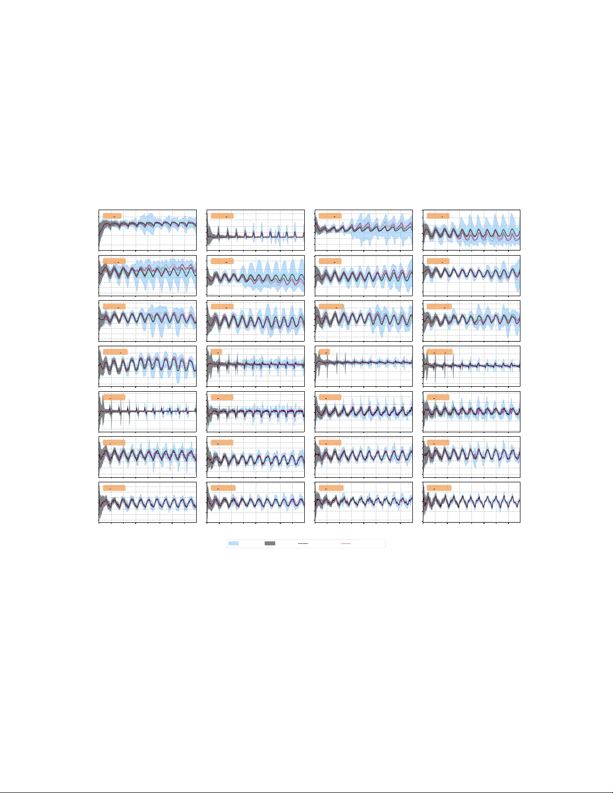
Proceedings of Machine Learning Research vol vvv: 1 – 28 , 2026 Scalable Data-Driv en Reachability Analysis and Contr ol via K oopman Operators with Conf ormal Cov erage Guarantees Dev esh Nath ∗ 1 D NAT H 7 @ G A T E C H . E D U Haoran Y in ∗ 1 H Y I N 9 5 @ G A T E C H . E D U Glen Chou 2 C H O U @ G A T E C H . E D U Geor gia Institute of T ec hnology . 1 School of ECE, 2 Schools of Cybersecurity & Privacy & Aer ospace Eng . Abstract W e propose a scalable reachability-based framework for probabilistic, data-driven safety veriﬁca- tion of unkno wn nonlinear dynamics. W e use K oopman theory with a neural network (NN) lifting function to learn an approximate linear representation of the dynamics and design linear controllers in this space to enable closed-loop tracking of a reference trajectory distribution. Closed-loop reachable sets are ef ﬁciently computed in the lifted space and mapped back to the original state space via NN veriﬁcation tools. T o capture model mismatch between the Koopman dynamics and the true system, we apply conformal prediction to produce statistically-valid error bounds that in- ﬂate the reachable sets to ensure the true trajectories are contained with a user-speciﬁed probability . These bounds generalize across references, enabling reuse without recomputation. Results on high- dimensional MuJoCo tasks (11D Hopper , 28D Swimmer) and 12D quadcopters show improv ed reachable set coverage rate, computational ef ﬁciency , and conservati veness ov er e xisting methods. Keyw ords: safety-critical control, reachability , K oopman operators, conformal prediction t = 0.00 s t = 0.66 s t = 1.33 s t = 1.99 s t = 2.66 s t = 3.32 s t = 3.99 s 0 5 Body Rot − 20 0 V el X − 25 0 V el Y Conformalized Koopman Reachable Set Reference Simulation Ground T ruth Rollouts Snapshots 0 . 0 2 . 5 Height z − 1 0 1 T orso Angle 2 4 Time (s) − 1 0 1 F oot Join t Figure 1: Executed trajectories / reachable sets for a 28D MuJoCo swimmer (a); 11D hopper (b). 1. Introduction Computing reachable sets, i.e., the set of states reachable over a time horizon, is key to robot safety . Ho we ver , reachability analysis for robots is difﬁcult as they often (i) lack analytical models, (ii) hav e high-dimensional nonlinear dynamics, and (iii) require reasoning ov er long horizons. Even if analytical dynamics are a vailable, challenges (ii) and (iii) cause nonlinear reachability tools ( Bansal et al. , 2017 ; Althof f , 2015 ) to become prohibiti ve or to suffer from excessiv e overapproximation © 2026 D. Nath, H. Y in & G. Chou. N AT H Y I N C H O U ov er long horizons ( Rober and Ho w , 2024 ). Data-dri ven reachability ( P ark et al. , 2024 ; Bak et al. , 2025 ) can be used without analytical models, b ut can be data-inef ﬁcient or lack guarantees that the estimated sets contain all possible trajectories. In contrast, linear reachability scales to long horizons and high dimensions ( Bak et al. , 2019 ). The K oopman framew ork learns linear dynamics in a lifted state space, e.g., via neural networks (NNs), to approximate the nonlinear system ( Shi et al. , 2024 ). While computing reachable sets for the Koopman linearization can be more scalable than using the original nonlinear dynamics, existing methods only provide guarantees for the approximate lifted dynamics. Thus, safety may not hold for the true system ( Bak et al. , 2021 , 2025 ). Moreover , existing K oopman reachability methods analyze a single dynamical system. Ho we ver , robots often require multiple controllers to complete dif ferent tasks, which forces existing methods to recompute reach- able sets from scratch for each new controller , which is inefﬁcient. Reusing previously computed information would enable more ef ﬁcient reachability analysis across controllers. T o close these gaps in scalability , speed, and reusability , we propose ScaRe-Kro (Scalable Reachability via Koopman Operators), which uses Koopman theory with an NN lifting function to perform reachability analysis and control. Unlik e prior Koopman reachability methods for au- tonomous systems, we also design a linear controller in this lifted space to track a distribution of reference trajectories, each completing a different task. ScaRe-Kro ef ﬁciently computes closed-loop reachable sets under the induced linear tracking err or dynamics in the lifted Koopman space and maps them to the original state space via NN veriﬁcation tools. T o account for K oopman model error , we apply conformal prediction (CP) to deri ve statistically-v alid error bounds. By inﬂating the mapped reachable sets with these CP bounds, they are guaranteed to contain the true system tra- jectories with a user-speciﬁed probability (e.g., 97.5%). Moreover , as the CP bounds are calibrated across the trajectory distrib ution, the y can be reused across different references and thus closed-loop systems, unlike prior Koopman approaches that certify only a single autonomous system. Overall, using linear reachability and CP , our method enables scalable data-dri ven probabilistic veriﬁcation and control, impro ving both efﬁcienc y and conserv ati veness over prior w ork. Our contrib utions are: 1. A scalable Koopman-based reachability framew ork for unknown nonlinear dynamics, using NN lifting functions and NN v eriﬁcation to estimate reachable sets in the original state space. 2. An approach for inﬂating the resulting Koopman reachable sets using CP , to obtain proba- bilistic guarantees of ov erapproximation for the true dynamics. 3. Control design in the lifted space for closed-loop tracking of a reference trajectory distribu- tion, with CP-based inﬂation bounds calibrated to be reusable across the distribution. 4. Extensi ve ev aluation, sho wing reliable veriﬁcation for high-dimensional robotic systems (up to 28D), outperforming baselines in safety rate, computation speed, and conserv ati veness. 2. Related W ork Reachability via Linear Relaxation While exact reachable set computation for nonlinear sys- tems is typically intractable, reachable set ov erapproximations (RSO As) can often be efﬁciently computed to certify safety ( Althoff et al. , 2021 ). When the closed-loop system in volv es NN com- ponents (e.g., learned dynamics or controller), RSO As can be computed via linear relaxation-based NN v eriﬁcation (NNV) tools (e.g., CR OWN ( Zhang et al. , 2018 )) ( Zhang et al. , 2018 ; Ev erett et al. , 2021 ; Jaf arpour et al. , 2024 ). Here, conserv ati veness grows with the number of nonlinearities ( Nath et al. , 2025 ) and can be excessi ve for nonlinear robot dynamics. Symbolic and one-shot methods 2 S C A L A B L E K O O P M A N R E AC H A B I L I T Y W I T H C O N F O R M A L C OV E R A G E G UA R A N T E E S mitigate this b ut raise runtime and memory costs ( Chen et al. , 2023 ; Rober and Ho w , 2024 ; Everett et al. , 2021 ). W e instead model the robot with K oopman-linearized dynamics, reducing the number of nonlinearities in the CG and improving scalability (i.e., computation time, conserv ativ eness). K oopman Reachability K oopman ( K oopman and Neumann , 1932 ) and Carleman ( Amini et al. , 2021 ; Bayer and Leine , 2023 ) linearizations accelerate reachability but introduce approximation error . Moreover , while error bounds exist, these deriv ations are limited to quadratic or polynomial dynamics ( Liu et al. , 2021 ; Forets and Pouly , 2017 ; Amini et al. , 2021 ), which do not apply to many robot dynamics models. Prior K oopman reachability methods also lack reachable set cov erage cal- ibration ( Thapliyal and Hwang , 2022 ) or guarantee containment only for a ﬁnite set of observed trajectories ( Kochdumper and Bak , 2022 ), f ailing to ensure safety for pre viously-unseen trajectories of the true system. Prior methods also do not support NN liftings and consider autonomous systems, which corresponds to ﬁxing a single controller . Changing controllers, as often done in robotics, re- quires repeating the calibration ( Forets and Schilling , 2021 ; Bak et al. , 2021 , 2025 ), which is inef ﬁ- cient. In contrast, we support NN liftings, provide probabilistic cov erage guarantees for the true dy- namics, and inte grate control design, enabling data-efﬁcient reachability across multiple controllers. Data-Driven Reachability Data-driv en reachability uses black-box trajectory data. Some meth- ods adapt Hamilton-Jacobi analysis ( Chilakamarri et al. , 2024 ), but this is costly for high-dimensional systems. Others learn reachability functions ( Sun and Mitra , 2022 ) but require dense data to accu- rately generalize, or yield ellipsoidal RSOAs ( Park et al. , 2024 ) assuming privileged system data (e.g., Lipschitz constants). Sampling-based methods ( Le w et al. , 2022 ) are limited to short hori- zons. Scenario optimization provides probabilistic guarantees ( Dietrich et al. , 2024 ) but is slower than K oopman-based methods ( Bak et al. , 2025 ). Moreov er, these methods assume a ﬁxed con- troller , yet robots often switch controllers to achiev e dif ferent goals, altering the closed-loop dynam- ics and forcing reachable sets to be recomputed. T rajectory-tracking reachability provides reusable tracking-error sets across reference trajectories ( Herbert et al. , 2017 ; Singh et al. , 2018 ; Knuth et al. , 2021 ). Data-driv en variants learn contraction metrics ( Chou et al. , 2021 , 2022 ; Knuth et al. , 2023 ) for tracking-based reachability of unknown systems, but ﬁnding such metrics is generally difﬁcult. W e b uild on this work, yielding K oopman reachable sets that are fast to compute, scalable to long horizons, and reusable for v arious closed-loop dynamics induced by tracking dif ferent trajectories. 3. Preliminaries W e consider unkno wn, black-box nonlinear systems, either in open-loop ( 1a ) or closed-loop ( 1b ): x t +1 = f ( x t , u t ) , (1a) x t +1 = f ( x t , π ( x t , t )) . = ˜ f ( x t ) , (1b) with timestep t ∈ { 0 , . . . , T } . = T , state x t ∈ X ⊆ R n , control u t ∈ U ⊆ R m , and feedback control law π : X × T → U . The initial state x 0 lies in set X 0 ⊆ X . Denote Int ( a, a ) = { a | a ≤ a ≤ a } , as an interval, where a, a ∈ R A and inequalities hold element-wise, i.e., a i ≤ a i ≤ a i , 1 ≤ i ≤ A . Denote the a -ball as B a ( c ) . = { x | ∥ x − c ∥ ∞ ≤ a } and sequence q 1: Q . = { q 1 , q 2 , . . . , q Q } = { q i } Q i =1 . W e use ⊕ and ⊖ to denote the Minko wski sum and difference, respecti vely . K oopman Operators As our work relies on K oopman operators, we discuss the basic concepts here. Consider autonomous discrete-time nonlinear dynamics x t +1 = f ( x t ) . A Koopman operator K is an inﬁnite-dimensional linear operator that e volv es the observ ables ϕ ∞ of the state K ϕ ∞ ( x ) = 3 N AT H Y I N C H O U ϕ ∞ ◦ f ( x ) according to ϕ ∞ ( x t +1 ) = K ϕ ∞ ( x t ) , where ◦ denotes function composition. As inﬁnite- dimensional K oopman operators are intractable to obtain in practice, we deﬁne an approximation to K using a ﬁnite-dimensional lifting function ϕ : X → Z ⊆ R l and matrix K A ∈ R l × l , which deﬁne lifted dynamics z t +1 = K A z t , where z t = ϕ ( x t ) is the lifted state and z t ∈ Z ⊆ R l . Here, l can be arbitrarily selected by the choice of the lifting function ϕ . For systems with control input ( 1a ), the lifted dynamics can be similarly written as z t +1 = K A z t + K B u t , where K B ∈ R l × m . In practice, ϕ , K A , and K B can be learned from data, with the lifting function g parameterized using polynomials or NNs ( Shi et al. , 2024 ). In this work, we utilize an NN-based autoencoder architecture, where the encoder ϕ : X → Z deﬁnes the lifting function and the decoder ψ : Z → ˆ X deﬁnes its learned in verse, i.e., ψ ( ϕ ( x )) ≈ x ; if ψ is a perfect in verse, ψ ( ϕ ( x )) = x and ˆ X = X . Reachability via NN V eriﬁcation (NNV) W e use NNV to compute reachable sets for closed- loop systems in volving NN-based lifting and in verse functions. NNV tools represent an NN as a computational graph (CG) – a directed ac yclic graph encoding the sequence of operations applied to an input ( Rober and Ho w , 2024 ). For some CG G with input set S ⊆ R n i and output G ( S ) ⊆ R n o , we can compute a guaranteed ov erapproximation of its image G ( S ) using CRO WN-based ( Zhang et al. , 2018 ) tools like auto LiRPA ( Xu et al. , 2020 ). These tools provide guaranteed af ﬁne lower and upper bounds, G and G , on the output G ( S ) for any interv al S , formalized in this proposition: Proposition 1 (CG Rob ustness ( Xu et al. , 2020 )) F or some CG G and interval S . = { s ∈ R n i | s ≤ s ≤ s } , ther e are af ﬁne functions G , G such that ∀ s ∈ S , G ( s ) ≤ G ( s ) ≤ G ( s ) . The inequali- ties hold element-wise and G ( s ) = Ψ s + α , G ( s ) = Φ s + β , with Ψ , Φ ∈ R n o × n i and α, β ∈ R n o . Gi ven controller π , dynamics ( 1a ), and initial set X 0 , the T -timestep exact reachable set is denoted as X 0: T . = {X 0 , f ( X t , π ( X t , t )) } T − 1 t =0 } . While exact reachability analysis is generally intractable for nonlinear systems ( Althof f et al. , 2021 ), it is often feasible to compute a reachable set ov erapproxi- mation (RSO A) X 0: T , which satisﬁes X t ⊆ X t for all t ∈ { 0 , . . . , T } . T o obtain X 0: T , Prop. 1 can be applied to the CG F of the T -step composition ˜ f T ( · ) . = ˜ f ◦ · · · ◦ ˜ f ( · ) of the closed-loop dynamics ˜ f ( 1b ), i.e., F ( x 0 ) . = { ˜ f ( x t ) . = f ( x t , π ( x t , t )) } T t =0 , with auto LiRPA computing the RSO A. Conf ormal Prediction (CP) Our RSOA computations also rely on CP . In this work, we adopt split CP , which partitions i.i.d. input-output pairs ( v ( i ) , y ( i ) ) ∈ V ×Y from a dataset D . = { ( v ( i ) , y ( i ) ) } L + K i =1 into a size- L training set D T and a size- K calibration set D C . For a gi ven prediction function µ : V → Y , we compute a nonconformity score R ( i ) . = s ( y ( i ) , µ ( v ( i ) )) for each of the K calibration pairs in D C , where s : Y × Y → R ≥ 0 is a chosen nonconformity score function. As an exam- ple, we can express the ℓ 2 prediction error of a learned dynamics model ˆ f in this framework by deﬁning v = ( x t , u t ) , y = x t +1 , µ ( v ) = ˆ f ( v ) , and s ( y , µ ( v )) = ∥ y − µ ( v ) ∥ 2 . Giv en a miscov- erage le vel δ ∈ (0 , 1) , a threshold C is deﬁned as the ( 1 − δ )-quantile of the calibration scores, C . = Quantile 1 − δ ( R (1) , . . . , R ( K ) , ∞ ) . This threshold deﬁnes the prediction set Y ( v ) . = { y ∈ Y | s ( y , µ ( v )) ≤ C } , which satisﬁes the marginal coverage guarantee P ( y (0) ∈ Y ( v (0) )) ≥ 1 − δ for an unseen data-point ( y (0) , v (0) ) that is exchangeable with D ( Lindemann et al. , 2024 ). 4. Problem Statement W e are giv en black-box access to f ( 1a ), i.e., we do not know its analytical form and its output can only be estimated via data. W e are a planner P : X → X T +1 × U T that generates open-loop refer- ence trajectories ( x ref 0: T , u ref 0: T − 1 ) that satisfy ( 1a ), starting from an initial condition x ref 0 ∈ X 0 ⊖ B ϵ (0) 4 S C A L A B L E K O O P M A N R E AC H A B I L I T Y W I T H C O N F O R M A L C OV E R A G E G UA R A N T E E S that is uniformly distributed over X 0 ⊖ B ϵ (0) . W e assume nothing further about P ; it can be a learned or traditional planner . At runtime, the true initial state x 0 may be perturbed from x ref 0 , i.e., x 0 ∈ B ϵ ( x ref 0 ) , where x 0 is uniformly distributed over B ϵ ( x ref 0 ) . T o be rob ust to this error, we design a con- troller π : X × T → U that tracks references from P and compute high-probability RSOAs X 0: T for the resulting closed-loop dynamics ( 1b ), such that P  V T t =0 ( x t ∈ X t )  ≥ 1 − δ . This process should scale to high-dimensional nonlinear systems over long horizons (e.g., n ≥ 25 , T ≥ 200 ). W e solve: Problem 1 (Model lear ning & controller design) Given N length- ( T +1) open-loop , dynamically- feasible trajectories generated by P via black-box queries of ( 1a ) , forming dataset D = { ( x ( i ) 0: T , u ( i ) 0: T − 1 } N i =1 , (a) train a K oopman model ( ϕ, ψ , K A , K B ) and (b) use the K oopman model to design a time- varying trajectory-tr acking contr oller π : X × T → U to stabilize to r efer ences generated by P . Problem 2 (( 1 − δ )-conﬁdent RSO A computation) Given M length- ( T + 1) closed-loop trajec- tories generated by trac king r eferences fr om P with the contr oller π from Pr ob . 1 , compute a ( 1 − δ )- conﬁdent RSO A X 0: T for the closed-loop dynamics ( 1b ) , which guarantees for any random refer ence ( x r ef 0: T , u r ef 0: T − 1 ) pr oduced by the planner P with x r ef 0 ∈ X 0 and initial state x 0 ∈ B ϵ ( x r ef 0 ) , the closed- loop trajectory r emains in X 0: T with pr obability at least 1 − δ , i.e., P  V T t =0 ( x t ∈ X t )  ≥ 1 − δ . 5. Methodology Our method (Fig. 2 , Alg. 1 ) learns a K oopman operator (Sec. 5.1 ), uses it for control design (Sec. 5.2 ), performs fast linear reachability analysis on the closed-loop lifted Koopman dynamics (Sec. 5.3 ), and inﬂates these reachable sets via CP to obtain probabilistic cov erage guarantees (Sec. 5.4 ). 5.1. K oopman Operator T raining T o solve Prob . 1 , we train a Koopman operator model ( ϕ, ψ , K A , K B ) on a dataset D . = { ( x ( i ) 0: T , u ( i ) 0: T − 1 ) } N i =1 of open-loop trajectories from a planner P (details in Sec. 6 ). W e use a composite loss L = P N i =1 ( λ 1 L ( i ) 1 + λ 2 L ( i ) 2 ) . The ﬁrst term, L ( i ) 1 = P T j =0  ∥ x ( i ) j − ψ ( ϕ ( x ( i ) j )) ∥ 2 + ∥ ϕ ( x ( i ) j ) − ϕ ( ψ ( ϕ ( x ( i ) j ))) ∥ 2  , enforces autoencoder accuracy via state reconstruction error and a latent consistency loss. The sec- ond term, L ( i ) 2 = P t + H j = t +1  ∥ x ( i ) j − ψ ( ˇ z ( i ) j ) ∥ 2 + ∥ ϕ ( x ( i ) j ) − ˇ z ( i ) j ∥ 2  , where ˇ z ( i ) j . = K A ˇ z ( i ) j − 1 + K B u ( i ) j − 1 and ˇ z ( i ) 0 = ϕ ( x ( i ) 0 ) , is a multi-step (horizon H ) dynamics loss penalizing prediction errors from the linear model ( K A , K B ) in both latent and state space.The latent consistency term is crucial for long-horizon prediction accuracy . W e initialize K A as identity and K B with Xavier uniform, train via learning rate annealing and weight decay , and set ( ϕ, ψ ) to ha ve ReLU or GELU activ ations. 5.2. K oopman T racking LQR Design T o reliably imitate state/control reference trajectories generated by the planner P in the lifted state space Z , a tracking controller π is required to stabilize against initial condition perturbations x 0 − x ref 0 and to reject disturbances due to model error in the learned lifted dynamics z t +1 = K A z t + K B u t . T o obtain π , we use the linearity of the lifted dynamics to design a linear quadratic re gulator (LQR) that tracks trajectories in Z . Gi ven a reference state-space trajectory x ref 0: T produced by P , we map it to the lifted state space as z ref 0: T . = { ϕ ( x ref t ) } T t =0 . The corresponding feedforward control trajectory u ref 0: T − 1 which minimizes the lifted-state imitation error is then computed as: u ref t = K † B ( z ref t +1 − K A z ref t ) , (2) 5 N AT H Y I N C H O U where K † B is the pseudo-in verse of K B . The error states δ z t = z t − z ref t and controls δ u t = u t − u ref t follo w linear error dynamics δ z t +1 = K A δ z t + K B δ u t , starting from an initial error δ z 0 = ϕ ( x 0 ) − z ref 0 , where x 0 ∈ B ϵ ( x ref 0 ) . W e solv e an LQR problem, ﬁnding the feedback controls δ u 0: T − 1 that minimize the ﬁnite-horizon quadratic cost δz ⊤ T Q T δ z T + P T − 1 t =0 ( δ z ⊤ t Qδ z t + δ u ⊤ t Rδ u t ) , subject to the linear dynamics δ z t +1 = K A δ z t + K B δ u t , where Q ≻ 0 , R ≻ 0 , and Q T ≻ 0 . In particular , we solve a backward Riccati recursion to obtain the optimal feedback gains G 0: T − 1 . This yields the tracking control law in the lifted state space ( 3 ), which can be applied on the nonlinear system ( 1a ) as ( 4 ) by measuring and encoding the state x t : u t = u ref t − G t ( z t − z ref t ) , (3) u t = u ref t − G t ( ϕ ( x t ) − z ref t ) . (4) 5.3. Reachability Analysis f or Closed-Loop K oopman Dynamics The high computational cost of nonlinear reachability motiv ates our use of Koopman operators. Standard RSO A computation repeatedly ov erapproximates nonlinearities at each timestep in both f and π (which typically must be nonlinear to stabilize f ), leading to high conservati veness. A T -step RSOA requires 2 T nonlinear function ev aluations, causing reachable sets to become vacu- ously loose as T increases. T o reduce conserv ati veness, partition-based methods split the input set X t , propagate each partition element, and union the result; howe ver , this incurs computational and memory costs that increases with the cardinality of the partition. In contrast, K oopman-based reach- ability improves scalability and reduces conserv ati veness without partitioning o verhead by reducing the number of nonlinearities. Mapping to the lifted space Z creates linear dynamics, eliminating the need to bound nonlinearities during propag ation. The linear dynamics also permit a linear track- ing controller . Consequently , computing an RSO A X t for any timestep t requires bounding only a single application of the nonlinear encoder ( ϕ ) and decoder ( ψ ), reducing the number of nonlinear bounding operations from 2 T to just 2 . T o apply this insight formally for RSO A computation, we deﬁne the T racking K oopman Feedback Loop (TKFL), denoted Γ , as a CG the describes the closed- loop dynamics for tracking z ref 0: T . = { ϕ ( x ref t ) } T t =0 in the lifted state space using the feedback control law ( 4 ). Speciﬁcally , the TKFL Γ : X 0 × U T × Z T +1 → ˆ X T +1 maps the initial state x 0 ∈ B ϵ ( x ref 0 ) , the feedforw ard control trajectory u ref 0: T − 1 ( 2 ), and the lifted reference z ref 0: T to the decoded trajectory ˆ x 0: T . = { ψ ( z t ) } T t =0 representing the predicted closed-loop trajectory ( 5 ) in the original state space, where the lifted states z t are updated via the closed-loop lifted dynamics ( 6 ): ˆ x 0: T = { x 0 , { ψ ( ˜ f z ( z t )) } T − 1 t =0 } , (5) z t +1 = K A z t + K B ( u ref t − G t ( z t − z ref t )) . = ˜ f z ( z t ) . (6) T o summarize, the CG is constructed as follows (see Fig. 2 for visualization). First, we map the initial state via ϕ into the latent space, computing z 0 = ϕ ( x 0 ) . Second, we unroll the T -fold recur- si ve application of the single-step latent dynamics, z t +1 = K A z t + K B u t , where u t is the closed- loop tracking control computed using ( 3 ), to obtain the latent trajectory z 0: T = { z 0 , z 2 , · · · , z T } . Third, z 0: T is mapped back to the original state space via the decoder ψ to obtain ˆ x 0: T . The CG Γ is passed to the auto LiRPA library ( Xu et al. , 2020 ), which enables set-based bound propaga- tion through Γ using CRO WN ( Zhang et al. , 2018 ). auto LiRPA computes vector -valued afﬁne bounding functions, Γ and Γ , which enables us to compute an RSOA ˆ X 0: T for the decoded closed- loop lifted dynamics ( 5 ) by considering speciﬁc components of Γ , Γ t and Γ t , that bound the states 6 S C A L A B L E K O O P M A N R E AC H A B I L I T Y W I T H C O N F O R M A L C OV E R A G E G UA R A N T E E S laten t input set, reference generation reference controller generation samples Koopman LQR Koopman dynamics target nonlinear system Koopman reachable set (KRS) conformal prediction AAAB/XicbVDJSgNBEO1xjXEbl5uXwSB4CjPihqegF48RskEyhp5OTdKkZ6G7RhKHwV/x4kERr/6HN//GznLQxAcFj/eqqKrnxYIrtO1vY2FxaXllNbeWX9/Y3No2d3ZrKkokgyqLRCQbHlUgeAhV5CigEUuggSeg7vVvRn79AaTiUVjBYQxuQLsh9zmjqKW2uT9op/ZVJbtvIQxQBqkEP2ubBbtoj2HNE2dKCmSKctv8anUilgQQIhNUqaZjx+imVCJnArJ8K1EQU9anXWhqGtIAlJuOr8+sI610LD+SukK0xurviZQGSg0DT3cGFHtq1huJ/3nNBP1LN+VhnCCEbLLIT4SFkTWKwupwCQzFUBPKJNe3WqxHJWWoA8vrEJzZl+dJ7aTonBfP7k4LpetpHDlyQA7JMXHIBSmRW1ImVcLII3kmr+TNeDJejHfjY9K6YExn9sgfGJ8/BU+VnQ== x ref 0: T AAAB/XicbVDJSgNBEO1xjXEbl5uXwSB4CjPihqegF48RskEyhp5OTdKkZ6G7RhKHwV/x4kERr/6HN//GznLQxAcFj/eqqKrnxYIrtO1vY2FxaXllNbeWX9/Y3No2d3ZrKkokgyqLRCQbHlUgeAhV5CigEUuggSeg7vVvRn79AaTiUVjBYQxuQLsh9zmjqKW2uT9op/ZVJbtvIQxQBqkEP2ubBbtoj2HNE2dKCmSKctv8anUilgQQIhNUqaZjx+imVCJnArJ8K1EQU9anXWhqGtIAlJuOr8+sI610LD+SukK0xurviZQGSg0DT3cGFHtq1huJ/3nNBP1LN+VhnCCEbLLIT4SFkTWKwupwCQzFUBPKJNe3WqxHJWWoA8vrEJzZl+dJ7aTonBfP7k4LpetpHDlyQA7JMXHIBSmRW1ImVcLII3kmr+TNeDJejHfjY9K6YExn9sgfGJ8/BU+VnQ== x ref 0: T AAAB/XicbVDJSgNBEO1xjXEbl5uXwSB4CjPihqegF48RskEyhp5OTdKkZ6G7RkyGwV/x4kERr/6HN//GznLQxAcFj/eqqKrnxYIrtO1vY2FxaXllNbeWX9/Y3No2d3ZrKkokgyqLRCQbHlUgeAhV5CigEUuggSeg7vVvRn79AaTiUVjBQQxuQLsh9zmjqKW2uT9sp/ZVJbtvITyiDFIJftY2C3bRHsOaJ86UFMgU5bb51epELAkgRCaoUk3HjtFNqUTOBGT5VqIgpqxPu9DUNKQBKDcdX59ZR1rpWH4kdYVojdXfEykNlBoEnu4MKPbUrDcS//OaCfqXbsrDOEEI2WSRnwgLI2sUhdXhEhiKgSaUSa5vtViPSspQB5bXITizL8+T2knROS+e3Z0WStfTOHLkgBySY+KQC1Iit6RMqoSRIXkmr+TNeDJejHfjY9K6YExn9sgfGJ8/CH2Vnw== z ref 0: T AAAB/XicbVDJSgNBEO1xjXEbl5uXwSB4CjPihqegF48RskEyhp5OTdKkZ6G7RkyGwV/x4kERr/6HN//GznLQxAcFj/eqqKrnxYIrtO1vY2FxaXllNbeWX9/Y3No2d3ZrKkokgyqLRCQbHlUgeAhV5CigEUuggSeg7vVvRn79AaTiUVjBQQxuQLsh9zmjqKW2uT9sp/ZVJbtvITyiDFIJftY2C3bRHsOaJ86UFMgU5bb51epELAkgRCaoUk3HjtFNqUTOBGT5VqIgpqxPu9DUNKQBKDcdX59ZR1rpWH4kdYVojdXfEykNlBoEnu4MKPbUrDcS//OaCfqXbsrDOEEI2WSRnwgLI2sUhdXhEhiKgSaUSa5vtViPSspQB5bXITizL8+T2knROS+e3Z0WStfTOHLkgBySY+KQC1Iit6RMqoSRIXkmr+TNeDJejHfjY9K6YExn9sgfGJ8/CH2Vnw== z ref 0: T AAAB9HicbVDLSgMxFL3js9ZX1aWbYBFclRnxtSy6cVnBPqAdSiZN29BMZkzuFMrQ73DjQhG3fow7/8ZMOwttPRA4nHMv9+QEsRQGXffbWVldW9/YLGwVt3d29/ZLB4cNEyWa8TqLZKRbATVcCsXrKFDyVqw5DQPJm8HoLvObY66NiNQjTmLuh3SgRF8wilbyOyHFIaMybU27brdUdivuDGSZeDkpQ45at/TV6UUsCblCJqkxbc+N0U+pRsEknxY7ieExZSM64G1LFQ258dNZ6Ck5tUqP9CNtn0IyU39vpDQ0ZhIGdjILaRa9TPzPayfYv/FToeIEuWLzQ/1EEoxI1gDpCc0ZyokllGlhsxI2pJoytD0VbQne4peXSeO84l1VLh8uytXbvI4CHMMJnIEH11CFe6hBHRg8wTO8wpszdl6cd+djPrri5DtH8AfO5w/CqZIb X 0 AAAB9HicbVDLSgMxFL1TX7W+qi7dBIvgqsyIr2XRjcsK9oHtUDJppg3NJGOSKZSh3+HGhSJu/Rh3/o2ZdhbaeiBwOOde7skJYs60cd1vp7Cyura+UdwsbW3v7O6V9w+aWiaK0AaRXKp2gDXlTNCGYYbTdqwojgJOW8HoNvNbY6o0k+LBTGLqR3ggWMgINlbyuxE2Q4J5+jjtub1yxa26M6Bl4uWkAjnqvfJXty9JElFhCMdadzw3Nn6KlWGE02mpm2gaYzLCA9qxVOCIaj+dhZ6iE6v0USiVfcKgmfp7I8WR1pMosJNZSL3oZeJ/Xicx4bWfMhEnhgoyPxQmHBmJsgZQnylKDJ9YgoliNisiQ6wwMbanki3BW/zyMmmeVb3L6sX9eaV2k9dRhCM4hlPw4ApqcAd1aACBJ3iGV3hzxs6L8+58zEcLTr5zCH/gfP4AxbeSHQ== Z 0 AAAB9HicbVDLSgMxFL3js9ZX1aWbYBFclRnxtSy6cVnBPqAdSiZN29BMZkzuFMrQ73DjQhG3fow7/8ZMOwttPRA4nHMv9+QEsRQGXffbWVldW9/YLGwVt3d29/ZLB4cNEyWa8TqLZKRbATVcCsXrKFDyVqw5DQPJm8HoLvObY66NiNQjTmLuh3SgRF8wilbyOyHFIaMybU27brdUdivuDGSZeDkpQ45at/TV6UUsCblCJqkxbc+N0U+pRsEknxY7ieExZSM64G1LFQ258dNZ6Ck5tUqP9CNtn0IyU39vpDQ0ZhIGdjILaRa9TPzPayfYv/FToeIEuWLzQ/1EEoxI1gDpCc0ZyokllGlhsxI2pJoytD0VbQne4peXSeO84l1VLh8uytXbvI4CHMMJnIEH11CFe6hBHRg8wTO8wpszdl6cd+djPrri5DtH8AfO5w/CqZIb X 0 AAAB/3icbVDJSgNBEO1xjXEbFbx4GQyCF8OMuOEp6MVjhGyQxNDTqUma9Cx014hhnIO/4sWDIl79DW/+jZ1kDpr4oODxXhVV9dxIcIW2/W3MzS8sLi3nVvKra+sbm+bWdk2FsWRQZaEIZcOlCgQPoIocBTQiCdR3BdTdwfXIr9+DVDwMKjiMoO3TXsA9zihqqWPuxp3EvqwcOeldC+EBpZ9I8NKOWbCL9hjWLHEyUiAZyh3zq9UNWexDgExQpZqOHWE7oRI5E5DmW7GCiLIB7UFT04D6oNrJ+P7UOtBK1/JCqStAa6z+nkior9TQd3WnT7Gvpr2R+J/XjNG7aCc8iGKEgE0WebGwMLRGYVhdLoGhGGpCmeT6Vov1qaQMdWR5HYIz/fIsqR0XnbPi6e1JoXSVxZEje2SfHBKHnJMSuSFlUiWMPJJn8krejCfjxXg3Piatc0Y2s0P+wPj8AeLBlgw= u ref 0: T  1 AAAB+3icbVDLSsNAFJ34rPUV69JNsAiuSiK+lkU3LivYB7QxTKY37dDJg5kbaQn5FTcuFHHrj7jzb5y2WWjrgQuHc+7l3nv8RHCFtv1trKyurW9slrbK2zu7e/vmQaWl4lQyaLJYxLLjUwWCR9BEjgI6iQQa+gLa/uh26refQCoeRw84ScAN6SDiAWcUteSZldTLMH/sIYxRhpmEIPfMql2zZ7CWiVOQKinQ8MyvXj9maQgRMkGV6jp2gm5GJXImIC/3UgUJZSM6gK6mEQ1Budns9tw60UrfCmKpK0Jrpv6eyGio1CT0dWdIcagWvan4n9dNMbh2Mx4lKULE5ouCVFgYW9MgrD6XwFBMNKFMcn2rxYZUUoY6rrIOwVl8eZm0zmrOZe3i/rxavyniKJEjckxOiUOuSJ3ckQZpEkbG5Jm8kjcjN16Md+Nj3rpiFDOH5A+Mzx8+w5U8 u ref t AAAB6nicbVDLSgNBEOyNrxhfUY9eBoPgKeyKr2PQi8eI5gHJEmYns8mQ2dllplcISz7BiwdFvPpF3vwbJ8keNLGgoajqprsrSKQw6LrfTmFldW19o7hZ2tre2d0r7x80TZxqxhsslrFuB9RwKRRvoEDJ24nmNAokbwWj26nfeuLaiFg94jjhfkQHSoSCUbTSQ9rDXrniVt0ZyDLxclKBHPVe+avbj1kacYVMUmM6npugn1GNgkk+KXVTwxPKRnTAO5YqGnHjZ7NTJ+TEKn0SxtqWQjJTf09kNDJmHAW2M6I4NIveVPzP66QYXvuZUEmKXLH5ojCVBGMy/Zv0heYM5dgSyrSwtxI2pJoytOmUbAje4svLpHlW9S6rF/fnldpNHkcRjuAYTsGDK6jBHdShAQwG8Ayv8OZI58V5dz7mrQUnnzmEP3A+fwBv6o3q u t AAAB6nicbVDLSgNBEOyNrxhfUY9eBoPgKeyKr2PQi8eI5gHJEmYns8mQ2dllplcISz7BiwdFvPpF3vwbJ8keNLGgoajqprsrSKQw6LrfTmFldW19o7hZ2tre2d0r7x80TZxqxhsslrFuB9RwKRRvoEDJ24nmNAokbwWj26nfeuLaiFg94jjhfkQHSoSCUbTSQ9rDXrniVt0ZyDLxclKBHPVe+avbj1kacYVMUmM6npugn1GNgkk+KXVTwxPKRnTAO5YqGnHjZ7NTJ+TEKn0SxtqWQjJTf09kNDJmHAW2M6I4NIveVPzP66QYXvuZUEmKXLH5ojCVBGMy/Zv0heYM5dgSyrSwtxI2pJoytOmUbAje4svLpHlW9S6rF/fnldpNHkcRjuAYTsGDK6jBHdShAQwG8Ayv8OZI58V5dz7mrQUnnzmEP3A+fwBv6o3q u t AAAB6nicbVDLSgNBEOyNrxhfUY9eBoPgKeyKr2PQi8eI5gHJEmYns8mQ2dllpleISz7BiwdFvPpF3vwbJ8keNFrQUFR1090VJFIYdN0vp7C0vLK6VlwvbWxube+Ud/eaJk414w0Wy1i3A2q4FIo3UKDk7URzGgWSt4LR9dRvPXBtRKzucZxwP6IDJULBKFrp7rGHvXLFrbozkL/Ey0kFctR75c9uP2ZpxBUySY3peG6CfkY1Cib5pNRNDU8oG9EB71iqaMSNn81OnZAjq/RJGGtbCslM/TmR0ciYcRTYzoji0Cx6U/E/r5NieOlnQiUpcsXmi8JUEozJ9G/SF5ozlGNLKNPC3krYkGrK0KZTsiF4iy//Jc2TqndePbs9rdSu8jiKcACHcAweXEANbqAODWAwgCd4gVdHOs/Om/M+by04+cw+/ILz8Q13iI3v z t AAAB6nicbVDLSgNBEOyNrxhfUY9eBoPgKeyKr2PQi8eI5gHJEmYns8mQ2dllpleISz7BiwdFvPpF3vwbJ8keNFrQUFR1090VJFIYdN0vp7C0vLK6VlwvbWxube+Ud/eaJk414w0Wy1i3A2q4FIo3UKDk7URzGgWSt4LR9dRvPXBtRKzucZxwP6IDJULBKFrp7rGHvXLFrbozkL/Ey0kFctR75c9uP2ZpxBUySY3peG6CfkY1Cib5pNRNDU8oG9EB71iqaMSNn81OnZAjq/RJGGtbCslM/TmR0ciYcRTYzoji0Cx6U/E/r5NieOlnQiUpcsXmi8JUEozJ9G/SF5ozlGNLKNPC3krYkGrK0KZTsiF4iy//Jc2TqndePbs9rdSu8jiKcACHcAweXEANbqAODWAwgCd4gVdHOs/Om/M+by04+cw+/ILz8Q13iI3v z t AAAB+XicbVC5TsNAEF1zhnAZKGksIiSqyEZcZQQNZZDIISXGWm/GySq7trU7jghW/oSGAoRo+RM6/obNUUDCk0Z6em9GM/PCVHCNrvttLS2vrK6tFzaKm1vbO7v23n5dJ5liUGOJSFQzpBoEj6GGHAU0UwVUhgIaYf9m7DcGoDRP4nscpuBL2o15xBlFIwW2/RTgQxvhEZXMFUSjwC65ZXcCZ5F4M1IiM1QD+6vdSVgmIUYmqNYtz03Rz6lCzgSMiu1MQ0pZn3ahZWhMJWg/n1w+co6N0nGiRJmK0ZmovydyKrUeytB0Soo9Pe+Nxf+8VobRlZ/zOM0QYjZdFGXCwcQZx+B0uAKGYmgIZYqbWx3Wo4oyNGEVTQje/MuLpH5a9i7K53dnpcr1LI4COSRH5IR45JJUyC2pkhphZECeySt5s3LrxXq3PqatS9Zs5oD8gfX5A3S2lDU= z ref t AAAB+XicbVC5TsNAEF1zhnAZKGksIiSqyEZcZQQNZZDIISXGWm/GySq7trU7jghW/oSGAoRo+RM6/obNUUDCk0Z6em9GM/PCVHCNrvttLS2vrK6tFzaKm1vbO7v23n5dJ5liUGOJSFQzpBoEj6GGHAU0UwVUhgIaYf9m7DcGoDRP4nscpuBL2o15xBlFIwW2/RTgQxvhEZXMFUSjwC65ZXcCZ5F4M1IiM1QD+6vdSVgmIUYmqNYtz03Rz6lCzgSMiu1MQ0pZn3ahZWhMJWg/n1w+co6N0nGiRJmK0ZmovydyKrUeytB0Soo9Pe+Nxf+8VobRlZ/zOM0QYjZdFGXCwcQZx+B0uAKGYmgIZYqbWx3Wo4oyNGEVTQje/MuLpH5a9i7K53dnpcr1LI4COSRH5IR45JJUyC2pkhphZECeySt5s3LrxXq3PqatS9Zs5oD8gfX5A3S2lDU= z ref t AAAB6nicbVDLSgNBEOyNrxhfUY9eBoPgKeyKr2PQgx4jmgckS5idzCZDZmeXmV4hLPkELx4U8eoXefNvnCR70GhBQ1HVTXdXkEhh0HW/nMLS8srqWnG9tLG5tb1T3t1rmjjVjDdYLGPdDqjhUijeQIGStxPNaRRI3gpG11O/9ci1EbF6wHHC/YgOlAgFo2il+5se9soVt+rOQP4SLycVyFHvlT+7/ZilEVfIJDWm47kJ+hnVKJjkk1I3NTyhbEQHvGOpohE3fjY7dUKOrNInYaxtKSQz9edERiNjxlFgOyOKQ7PoTcX/vE6K4aWfCZWkyBWbLwpTSTAm079JX2jOUI4toUwLeythQ6opQ5tOyYbgLb78lzRPqt559ezutFK7yuMowgEcwjF4cAE1uIU6NIDBAJ7gBV4d6Tw7b877vLXg5DP78AvOxzcp1o28 G t AAAB6nicbVDLSgNBEOyNrxhfUY9eBoPgKeyKr2PQgx4jmgckS5idzCZDZmeXmV4hLPkELx4U8eoXefNvnCR70GhBQ1HVTXdXkEhh0HW/nMLS8srqWnG9tLG5tb1T3t1rmjjVjDdYLGPdDqjhUijeQIGStxPNaRRI3gpG11O/9ci1EbF6wHHC/YgOlAgFo2il+5se9soVt+rOQP4SLycVyFHvlT+7/ZilEVfIJDWm47kJ+hnVKJjkk1I3NTyhbEQHvGOpohE3fjY7dUKOrNInYaxtKSQz9edERiNjxlFgOyOKQ7PoTcX/vE6K4aWfCZWkyBWbLwpTSTAm079JX2jOUI4toUwLeythQ6opQ5tOyYbgLb78lzRPqt559ezutFK7yuMowgEcwjF4cAE1uIU6NIDBAJ7gBV4d6Tw7b877vLXg5DP78AvOxzcp1o28 G t AAAB8nicbVDJSgNBEO1xjXGLevTSGIQIEmbE7Rj04jGCWWAyDD2dnqRJT/fQXSOGIZ/hxYMiXv0ab/6NneWgiQ8KHu9VUVUvSgU34LrfztLyyuraemGjuLm1vbNb2ttvGpVpyhpUCaXbETFMcMkawEGwdqoZSSLBWtHgduy3Hpk2XMkHGKYsSEhP8phTAlby48pTCKc4C+EkLJXdqjsBXiTejJTRDPWw9NXpKpolTAIVxBjfc1MIcqKBU8FGxU5mWErogPSYb6kkCTNBPjl5hI+t0sWx0rYk4In6eyIniTHDJLKdCYG+mffG4n+en0F8HeRcphkwSaeL4kxgUHj8P+5yzSiIoSWEam5vxbRPNKFgUyraELz5lxdJ86zqXVYv7s/LtZtZHAV0iI5QBXnoCtXQHaqjBqJIoWf0it4ccF6cd+dj2rrkzGYO0B84nz8m/pCI f ( x t ,u t ) AAAB7nicbVDLSgNBEOz1GeMr6tHLYBAEIeyKr2PQi8cI5gHJEmYns8mQ2dllplcMSz7CiwdFvPo93vwbJ8keNLGgoajqprsrSKQw6LrfztLyyuraemGjuLm1vbNb2ttvmDjVjNdZLGPdCqjhUiheR4GStxLNaRRI3gyGtxO/+ci1EbF6wFHC/Yj2lQgFo2il5lM3w1Nv3C2V3Yo7BVkkXk7KkKPWLX11ejFLI66QSWpM23MT9DOqUTDJx8VOanhC2ZD2edtSRSNu/Gx67pgcW6VHwljbUkim6u+JjEbGjKLAdkYUB2bem4j/ee0Uw2s/EypJkSs2WxSmkmBMJr+TntCcoRxZQpkW9lbCBlRThjahog3Bm395kTTOKt5l5eL+vFy9yeMowCEcwQl4cAVVuIMa1IHBEJ7hFd6cxHlx3p2PWeuSk88cwB84nz8S0I9p x t +1 AAAB7nicbVDLSgNBEOz1GeMr6tHLYBAEIeyKr2PQi8cI5gHJEmYns8mQ2dllpleISz7CiwdFvPo93vwbJ8keNLGgoajqprsrSKQw6LrfztLyyuraemGjuLm1vbNb2ttvmDjVjNdZLGPdCqjhUiheR4GStxLNaRRI3gyGtxO/+ci1EbF6wFHC/Yj2lQgFo2il5lM3w1Nv3C2V3Yo7BVkkXk7KkKPWLX11ejFLI66QSWpM23MT9DOqUTDJx8VOanhC2ZD2edtSRSNu/Gx67pgcW6VHwljbUkim6u+JjEbGjKLAdkYUB2bem4j/ee0Uw2s/EypJkSs2WxSmkmBMJr+TntCcoRxZQpkW9lbCBlRThjahog3Bm395kTTOKt5l5eL+vFy9yeMowCEcwQl4cAVVuIMa1IHBEJ7hFd6cxHlx3p2PWeuSk88cwB84nz8V5I9r z t +1 AAAB63icbVBNS8NAEJ3Ur1q/qh69LBbBU0nEqseiF48V7Ae0oWy2m2bp7ibsboQS+he8eFDEq3/Im//GTZuDtj4YeLw3w8y8IOFMG9f9dkpr6xubW+Xtys7u3v5B9fCoo+NUEdomMY9VL8CaciZp2zDDaS9RFIuA024wucv97hNVmsXy0UwT6gs8lixkBJtcGiQRG1Zrbt2dA60SryA1KNAaVr8Go5ikgkpDONa677mJ8TOsDCOcziqDVNMEkwke076lEguq/Wx+6wydWWWEwljZkgbN1d8TGRZaT0VgOwU2kV72cvE/r5+a8MbPmExSQyVZLApTjkyM8sfRiClKDJ9agoli9lZEIqwwMTaeig3BW355lXQu6t5VvfFwWWveFnGU4QRO4Rw8uIYm3EML2kAggmd4hTdHOC/Ou/OxaC05xcwx/IHz+QMWyI5J  AAAB63icbVBNS8NAEJ3Ur1q/qh69LBbBU0nEqseiF48V7Ae0oWy2m2bp7ibsboQS+he8eFDEq3/Im//GTZuDtj4YeLw3w8y8IOFMG9f9dkpr6xubW+Xtys7u3v5B9fCoo+NUEdomMY9VL8CaciZp2zDDaS9RFIuA024wucv97hNVmsXy0UwT6gs8lixkBJtcGiQRG1Zrbt2dA60SryA1KNAaVr8Go5ikgkpDONa677mJ8TOsDCOcziqDVNMEkwke076lEguq/Wx+6wydWWWEwljZkgbN1d8TGRZaT0VgOwU2kV72cvE/r5+a8MbPmExSQyVZLApTjkyM8sfRiClKDJ9agoli9lZEIqwwMTaeig3BW355lXQu6t5VvfFwWWveFnGU4QRO4Rw8uIYm3EML2kAggmd4hTdHOC/Ou/OxaC05xcwx/IHz+QMWyI5J  AAAB63icbVBNSwMxEJ2tX7V+VT16CRbBU9kVv45FLx4rWFtol5JNs21okg1JVihL/4IXD4p49Q9589+YbfegrQ8GHu/NMDMvUpwZ6/vfXmlldW19o7xZ2dre2d2r7h88miTVhLZIwhPdibChnEnassxy2lGaYhFx2o7Gt7nffqLasEQ+2ImiocBDyWJGsM2lnjKsX635dX8GtEyCgtSgQLNf/eoNEpIKKi3h2Jhu4CsbZlhbRjidVnqpoQqTMR7SrqMSC2rCbHbrFJ04ZYDiRLuSFs3U3xMZFsZMROQ6BbYjs+jl4n9eN7XxdZgxqVJLJZkvilOObILyx9GAaUosnziCiWbuVkRGWGNiXTwVF0Kw+PIyeTyrB5f1i/vzWuOmiKMMR3AMpxDAFTTgDprQAgIjeIZXePOE9+K9ex/z1pJXzBzCH3ifPyd/jlQ= AAAB63icbVBNSwMxEJ2tX7V+VT16CRbBU9kVv45FLx4rWFtol5JNs21okg1JVihL/4IXD4p49Q9589+YbfegrQ8GHu/NMDMvUpwZ6/vfXmlldW19o7xZ2dre2d2r7h88miTVhLZIwhPdibChnEnassxy2lGaYhFx2o7Gt7nffqLasEQ+2ImiocBDyWJGsM2lnjKsX635dX8GtEyCgtSgQLNf/eoNEpIKKi3h2Jhu4CsbZlhbRjidVnqpoQqTMR7SrqMSC2rCbHbrFJ04ZYDiRLuSFs3U3xMZFsZMROQ6BbYjs+jl4n9eN7XxdZgxqVJLJZkvilOObILyx9GAaUosnziCiWbuVkRGWGNiXTwVF0Kw+PIyeTyrB5f1i/vzWuOmiKMMR3AMpxDAFTTgDprQAgIjeIZXePOE9+K9ex/z1pJXzBzCH3ifPyd/jlQ= AAAB8XicbVDLSsNAFL3xWeur6tLNYBEqSEnE17LWjdBNBfvANoTJdNIOnUzCzEQooX/hxoUibv0bd/6N0zYLbT1w4XDOvdx7jx9zprRtf1tLyyura+u5jfzm1vbObmFvv6miRBLaIBGPZNvHinImaEMzzWk7lhSHPqctf3g78VtPVCoWiQc9iqkb4r5gASNYG+mxVPNuTlHNq554haJdtqdAi8TJSBEy1L3CV7cXkSSkQhOOleo4dqzdFEvNCKfjfDdRNMZkiPu0Y6jAIVVuOr14jI6N0kNBJE0Jjabq74kUh0qNQt90hlgP1Lw3Ef/zOokOrt2UiTjRVJDZoiDhSEdo8j7qMUmJ5iNDMJHM3IrIAEtMtAkpb0Jw5l9eJM2zsnNZvrg/L1aqWRw5OIQjKIEDV1CBO6hDAwgIeIZXeLOU9WK9Wx+z1iUrmzmAP7A+fwBDHI9c ( K A ,K B ) AAACAXicbVDLSsNAFJ3UV62vqBvBzWARXNSSiK9l0Y3LCn1BE8pkOm2HTiZh5kYooW78FTcuFHHrX7jzb5y2WWjrgQuHc+7l3nuCWHANjvNt5ZaWV1bX8uuFjc2t7R17d6+ho0RRVqeRiFQrIJoJLlkdOAjWihUjYSBYMxjeTvzmA1OaR7IGo5j5IelL3uOUgJE69gFgj0vspU4Je6IbgS7h2qnrjTt20Sk7U+BF4makiDJUO/aX141oEjIJVBCt264Tg58SBZwKNi54iWYxoUPSZ21DJQmZ9tPpB2N8bJQu7kXKlAQ8VX9PpCTUehQGpjMkMNDz3kT8z2sn0Lv2Uy7jBJiks0W9RGCI8CQO3OWKURAjQwhV3NyK6YAoQsGEVjAhuPMvL5LGWdm9LF/cnxcrN1kceXSIjtAJctEVqqA7VEV1RNEjekav6M16sl6sd+tj1pqzspl99AfW5w/SR5U4 t 2 { 0 ,...,T  1 } AAACAXicbVDLSsNAFJ3UV62vqBvBzWARXNSSiK9l0Y3LCn1BE8pkOm2HTiZh5kYooW78FTcuFHHrX7jzb5y2WWjrgQuHc+7l3nuCWHANjvNt5ZaWV1bX8uuFjc2t7R17d6+ho0RRVqeRiFQrIJoJLlkdOAjWihUjYSBYMxjeTvzmA1OaR7IGo5j5IelL3uOUgJE69gFgj0vspU4Je6IbgS7h2qnrjTt20Sk7U+BF4makiDJUO/aX141oEjIJVBCt264Tg58SBZwKNi54iWYxoUPSZ21DJQmZ9tPpB2N8bJQu7kXKlAQ8VX9PpCTUehQGpjMkMNDz3kT8z2sn0Lv2Uy7jBJiks0W9RGCI8CQO3OWKURAjQwhV3NyK6YAoQsGEVjAhuPMvL5LGWdm9LF/cnxcrN1kceXSIjtAJctEVqqA7VEV1RNEjekav6M16sl6sd+tj1pqzspl99AfW5w/SR5U4 t 2 { 0 ,...,T  1 } T times, T times, AAACAXicbVBLSwMxGMzWV62vVS+Cl2ARPJVd8YWnohePFfqC7rJk07QNzSZLkhXKsl78K148KOLVf+HNf2O23YO2DgSGmfmSfBPGjCrtON9WaWl5ZXWtvF7Z2Nza3rF399pKJBKTFhZMyG6IFGGUk5ammpFuLAmKQkY64fg29zsPRCoqeFNPYuJHaMjpgGKkjRTYB94I6dQTJpNfkXazLEid62YW2FWn5kwBF4lbkCoo0AjsL68vcBIRrjFDSvVcJ9Z+iqSmmJGs4iWKxAiP0ZD0DOUoIspPpxtk8NgofTgQ0hyu4VT9PZGiSKlJFJpkhPRIzXu5+J/XS/Tgyk8pjxNNOJ49NEgY1ALmdcA+lQRrNjEEYUnNXyEeIYmwNqVVTAnu/MqLpH1acy9q5/dn1fpNUUcZHIIjcAJccAnq4A40QAtg8AiewSt4s56sF+vd+phFS1Yxsw/+wPr8ASonl1s= ˆ X 0: T AAACFnicbVDLSgMxFM34rPVVdekmWIS6sMyILwSh6EZwU6EPodMOmTS1oZkHyR1pCfMVbvwVNy4UcSvu/BvTx0KrBy6cnHMvuff4seAKbPvLmpmdm19YzCxll1dW19ZzG5s1FSWSsiqNRCRvfaKY4CGrAgfBbmPJSOALVvd7l0O/fs+k4lFYgUHMmgG5C3mHUwJG8nL7rna7BHDf0/ZZJW3pAt9L3dTT/Nwxr+uWC6wPMtCUiDT1cnm7aI+A/xJnQvJogrKX+3TbEU0CFgIVRKmGY8fQ1EQCp4KlWTdRLCa0R+5Yw9CQBEw19eisFO8apY07kTQVAh6pPyc0CZQaBL7pDAh01bQ3FP/zGgl0Tpuah3ECLKTjjzqJwBDhYUa4zSWjIAaGECq52RXTLpGEgkkya0Jwpk/+S2oHRee4eHRzmC9dTOLIoG20gwrIQSeohK5QGVURRQ/oCb2gV+vRerberPdx64w1mdlCv2B9fAPMup/S { ˆ x ( i ) 0: T } K cal i =1 AAACEXicbVDJSgNBEO1xjXEb9ehlMAjxEmbEDUEIehG8RMgGmWTo6XSSJj0L3TWS0MwvePFXvHhQxKs3b/6NneWgiQ8KXr9XRVc9P+ZMgm1/GwuLS8srq5m17PrG5ta2ubNblVEiCK2QiEei7mNJOQtpBRhwWo8FxYHPac3v34z82gMVkkVhGYYxbQa4G7IOIxi05Jl5Vw08ZV+W05bKs6PUTT3Frhz9umu5QAcgAkUwT1PPzNkFewxrnjhTkkNTlDzzy21HJAloCIRjKRuOHUNTYQGMcJpm3UTSGJM+7tKGpiEOqGyq8UWpdaiVttWJhK4QrLH6e0LhQMph4OvOAENPznoj8T+vkUDnoqlYGCdAQzL5qJNwCyJrFI/VZoIS4ENNMBFM72qRHhaYgA4xq0NwZk+eJ9XjgnNWOL0/yRWvp3Fk0D46QHnkoHNURLeohCqIoEf0jF7Rm/FkvBjvxsekdcGYzuyhPzA+fwAr+Z3n { x ( i ) 0: T } K cal i =1 conformalized Koopman reachable set (CKRS) . AAAB/XicbVDLSsNAFL3xWeurPnZugkVwVRLxtSx147KCfUBTymR60w6dTMLMRKih+CtuXCji1v9w5984abPQ1gMDh3Pu5Z45fsyZ0o7zbS0tr6yurRc2iptb2zu7pb39pooSSbFBIx7Jtk8UciawoZnm2I4lktDn2PJHN5nfekCpWCTu9TjGbkgGggWMEm2kXunQC4keUsLT2qTnYawYz+SyU3GmsBeJm5My5Kj3Sl9eP6JJiEJTTpTquE6suymRmlGOk6KXKIwJHZEBdgwVJETVTafpJ/aJUfp2EEnzhLan6u+NlIRKjUPfTGZZ1byXif95nUQH192UiTjRKOjsUJBwW0d2VoXdZxKp5mNDCJXMZLXpkEhCtSmsaEpw57+8SJpnFfeycnF3Xq7W8joKcATHcAouXEEVbqEODaDwCM/wCm/Wk/VivVsfs9ElK985gD+wPn8AD3eVog== B ✏ AAAB8HicbVDLSgNBEOyNrxhfUY9eBoPgxbArvvAU9KDHCHlJsoTZyWwyZGZ2mZkVwpKv8OJBEa9+jjf/xkmyB00saCiquunuCmLOtHHdbye3tLyyupZfL2xsbm3vFHf3GjpKFKF1EvFItQKsKWeS1g0znLZiRbEIOG0Gw9uJ33yiSrNI1swopr7AfclCRrCx0uNdN3WvayfeuFssuWV3CrRIvIyUIEO1W/zq9CKSCCoN4VjrtufGxk+xMoxwOi50Ek1jTIa4T9uWSiyo9tPpwWN0ZJUeCiNlSxo0VX9PpFhoPRKB7RTYDPS8NxH/89qJCa/8lMk4MVSS2aIw4chEaPI96jFFieEjSzBRzN6KyAArTIzNqGBD8OZfXiSN07J3UT5/OCtVbrI48nAAh3AMHlxCBe6hCnUgIOAZXuHNUc6L8+58zFpzTjazD3/gfP4AiDaPmA== G 0: T  1 AAAB+3icbVDLSsNAFJ34rPUV69JNsAiuSiK+lkU3LivYB7QxTKY37dDJg5kbaQn5FTcuFHHrj7jzb5y2WWjrgQuHc+7l3nv8RHCFtv1trKyurW9slrbK2zu7e/vmQaWl4lQyaLJYxLLjUwWCR9BEjgI6iQQa+gLa/uh26refQCoeRw84ScAN6SDiAWcUteSZldTLMH/sIYxRhpmEIPfMql2zZ7CWiVOQKinQ8MyvXj9maQgRMkGV6jp2gm5GJXImIC/3UgUJZSM6gK6mEQ1Budns9tw60UrfCmKpK0Jrpv6eyGio1CT0dWdIcagWvan4n9dNMbh2Mx4lKULE5ouCVFgYW9MgrD6XwFBMNKFMcn2rxYZUUoY6rrIOwVl8eZm0zmrOZe3i/rxavyniKJEjckxOiUOuSJ3ckQZpEkbG5Jm8kjcjN16Md+Nj3rpiFDOH5A+Mzx8+w5U8 u ref t AAACEHicbVC7TsMwFHXKq5RXgJHFokKwUCWIl5gqWBiL1JfUhMhx3Naq40S2g1RF+QQWfoWFAYRYGdn4G5w2A7QcydLROffI9x4/ZlQqy/o2SguLS8sr5dXK2vrG5pa5vdOWUSIwaeGIRaLrI0kY5aSlqGKkGwuCQp+Rjj+6yf3OAxGSRrypxjFxQzTgtE8xUlryzEMn0naeTp0QqSFGLO1mmZdaV83sPrWPnYAwhTLPrFo1awI4T+yCVEGBhmd+OUGEk5BwhRmSsmdbsXJTJBTFjGQVJ5EkRniEBqSnKUchkW46OSiDB1oJYD8S+nEFJ+rvRIpCKcehryfzpeWsl4v/eb1E9S/dlPI4UYTj6Uf9hEEVwbwdGFBBsGJjTRAWVO8K8RAJhJXusKJLsGdPniftk5p9Xju7O63Wr4s6ymAP7IMjYIMLUAe3oAFaAINH8AxewZvxZLwY78bHdLRkFJld8AfG5w+8t52o X 1   0: T AAAB7nicbVDLSgNBEOz1GeMr6tHLYBAEIeyKr2PQi8cI5gHJEmYns8mQ2dllpleISz7CiwdFvPo93vwbJ8keNLGgoajqprsrSKQw6LrfztLyyuraemGjuLm1vbNb2ttvmDjVjNdZLGPdCqjhUiheR4GStxLNaRRI3gyGtxO/+ci1EbF6wFHC/Yj2lQgFo2il5lM3w1Nv3C2V3Yo7BVkkXk7KkKPWLX11ejFLI66QSWpM23MT9DOqUTDJx8VOanhC2ZD2edtSRSNu/Gx67pgcW6VHwljbUkim6u+JjEbGjKLAdkYUB2bem4j/ee0Uw2s/EypJkSs2WxSmkmBMJr+TntCcoRxZQpkW9lbCBlRThjahog3Bm395kTTOKt5l5eL+vFy9yeMowCEcwQl4cAVVuIMa1IHBEJ7hFd6cxHlx3p2PWeuSk88cwB84nz8V5I9r z t +1 Figure 2: A block diagram that describes the ﬂow of our method (ScaRe-Kro). Green and orange arro ws represent KRS and CP computations, respecti vely . reached under ( 5 ) at timestep t , starting from any initial condition x 0 ∈ X 0 . This resulting hyper- rectangular set ˆ X 0: T , which we refer to as the Koopman reachable set (KRS), is found by solving the optimization ( 7 ), which is computed ef ﬁciently by auto LiRPA : ˆ X 0: T . =  Int  min x 0 ∈X 0 Γ t ( x 0 , u ref 0: T − 1 , z ref 0: T ) , max x 0 ∈X 0 Γ t ( x 0 , u ref 0: T − 1 , z ref 0: T )  T t =0 (7) The KRS ˆ X 0: T ov erapproximates ˆ x 0: T so that ˆ x t ∈ ˆ X t , for all t ∈ T , ensuring the decoded closed- loop lifted dynamics ( 5 ) remain in ˆ X 0: T . Formally , we state the following result (proof in App. 8.1 ): Lemma 1 (KRS overappr oximation) Let Γ denote the closed-loop CG of TKFL, and let X 0 be the initial set. Suppose the KRS ˆ X 0: T is deﬁned as in ( 7 ) . Then, for any initial state x 0 ∈ X 0 , the decoded closed-loop trajectory ( 5 ) , i.e ., ˆ x 0: T = Γ( x 0 , z r ef 0: T , u r ef 0: T − 1 ) satisﬁes ˆ x t ∈ ˆ X t for all t ∈ T . Crucially , the KRS o verapproximates the reachable set for the decoded Koopman linearized dynam- ics ( 5 ), not the true nonlinear dynamics ( 1b ), due to K oopman model error . This moti vates Sec. 5.4 . 5.4. Conf ormalizing K oopman Reachable Sets W e now explain ho w to inﬂate the KRS to guarantee it contains the true system ( 1b ) trajectories with a user-speciﬁed probability 1 − δ . W e use CP to compute a high-probability upper bound on the state-space prediction error of the decoded closed-loop lifted dynamics ( 5 ). Speciﬁcally , we adapt the single nonconformity score approach (SNSA) ( Lindemann et al. , 2024 ) to compute state- and dimension-dependent error bounds using a calibration dataset D C = { ( x ( i ) 0: T , ˆ x ( i ) 0: T ) } K cal i =1 of tra- jectories of the true closed-loop dynamics x 0: T ( 1b ) and the decoded closed-loop lifted dynamics ˆ x 0: T ( 5 ). T o construct each data tuple in D C , we sample a reference trajectory x ref , ( i ) 0: T from planner P and an initial state x ( i ) 0 uniformly from B ϵ ( x ref 0 ) . W e then compute the latent reference trajectory z ref , ( i ) 0: T = { ϕ ( x ref , ( i ) t ) } T t =0 and the feedforward control sequence u ref , ( i ) 0: T − 1 using ( 2 ). W e use u ref , ( i ) 0: T − 1 to calculate the trajectory returned by 1) tracking z ref 0: T in the lifted state space ( 8 ) and decoding to the state space via ψ and 2) ex ecuting the K oopman controller on the true nonlinear dynamics ( 9 ): 7 N AT H Y I N C H O U ˆ x ( i ) 1: T =  ψ  K A z t + K B  u ref t − G t ( z t − z ref t )   T − 1 t =0 (8) x ( i ) 1: T = { f ( x t , u ref t − G t ( ϕ ( x t ) − z ref t ) } T − 1 t =0 (9) The prediction error for each state dimension j ∈ { 1 , . . . , n } at time t is denoted e ( i ) t,j = x ( i ) t,j − ˆ x ( i ) t,j . This giv es a calibration set of error trajectories D E = {{ e ( i ) t } T t =0 } K cal i =1 , where each e ( i ) t ∈ R n . Each error trajectory e ( i ) is normalized into a single non-conformity score R ( i ) = max t,j ( λ t,j | e ( i ) t,j | ) , which is the maximum weighted error ov er all time steps t ∈ { 0 , . . . , T } and state dimensions j ∈ { 1 , . . . , n } . Here, the normalization constant λ t,j . = 1 / ( e max t,j + σ ) ∈ R > 0 is computed using a separate normalization dataset D N . This dataset, D N , consists of M λ additional error trajectories, { e ( i ) } K cal + M λ i = K cal +1 , collected using the same process as the calibration data. Here, σ is a small positiv e constant to pre vent di vision by zero. The term e max t,j is the dimension-wise and time-wise maximum absolute error observed across D N , i.e., e max t,j = max i | e ( i ) t,j | where i ∈ { K cal + 1 , . . . , K cal + M } . No w , gi ven a user-deﬁned miscoverage rate δ ∈ (0 , 1) , we compute the (1 − δ ) quantile of the non-conformity scores C = Quantile 1 − δ ( { R ( i ) } K cal i =1 ∪ {∞} ) by ﬁnding the p -th smallest value of the scores { R ( i ) } K cal i =1 , where p ≡ ⌈ ( K cal + 1)(1 − δ ) ⌉ . The ﬁnal, time- and dimension-dependent error bound ¯ e t,j ∈ R ≥ 0 is obtained by re versing the normalization ¯ e t,j = C /λ t,j . These bounds en- sure that for an unseen test data-point ( x (0) 0: T , ˆ x (0) 0: T ) , the true prediction error | e (0) t,j | will be contained within the bound ¯ e t,j for all t and j , with probability at least 1 − δ , i.e., P  | e (0) t,j | ≤ ¯ e t,j , ∀ t ∈ { 0 , . . . , T } , ∀ j ∈ { 1 , . . . , n }  ≥ 1 − δ W e use these bounds to inﬂate the KRS computed in ( 7 ) to compute RSO As for the original closed- loop dynamics ( 1b ) that are v alid with probability at least 1 − δ , using ( 11 ) (proof in App. 8.1 ): Theorem 1 (CKRS Co verage Guarantee) Let ˆ X 0: T be the KRS deﬁned in ( 7 ) and let ¯ e t = [ ¯ e t, 1 , . . . , ¯ e t,n ] ⊤ ∈ R n . Deﬁne the conformalized K oopman r eachable set (CKRS) as X 1 − δ 0: T ≡  ˆ X t ⊕ diag ( ¯ e t ) B 1 (0)  T t =0 , (10) wher e diag( ¯ e t ) ∈ R n × n is a diagonal matrix with ¯ e t on its diagonal. Then, for a new r eference trajectory x r ef , (0) 0: T drawn fr om the same distribution, the CKRS contains the true closed-loop system trajectory g enerated by ( 1b ) with pr obability at least 1 − δ , i.e., P  V T t =0 x (0) t ∈ X 1 − δ t  ≥ 1 − δ . Ofﬂine Calibration As discussed so far , the method in Sec. 5.4 is reference-speciﬁc, as the calibration trajectories D C and error bounds ¯ e t hold speciﬁcally for a single reference x ref 0: T . W e propose an ofﬂine approach that pre-computes a single, global set of error bounds ¯ e t,j v alid for any reference x ref 0: T sampled from the planner P . This is done by building a larger , more div erse calibration set. W e ﬁrst sample N ref reference trajectories { x ref , ( i ) 0: T } N ref i =1 ∼ P . For each reference, we generate a calibration trajectory by sampling x ( i ) 0 ∼ B ϵ ( x ref , ( i ) 0 ) , yielding an error trajectory e ( i ) t = x ( i ) t − ˆ x ( i ) t , where x ( i ) t and ˆ x ( i ) t are as deﬁned in ( 8 ) and ( 9 ), respectiv ely . The SNSA procedure (computing R ( i ) , C , and ¯ e t,j via λ t,j ) is then performed exactly once on this entire aggre gated set. At runtime, giv en a new reference x ref , (0) 0: T sampled from P , two efﬁcient computations are per- formed: 1) we compute the nominal KRS ˆ X 0: T speciﬁc to x ref , (0) 0: T via ( 7 )), and 2) we inﬂate this set using the pre-computed of ﬂine bounds ¯ e t via the Minko wski sum X 1 − δ t = ˆ X t ⊕ diag ( ¯ e t ) B 1 (0) , 8 S C A L A B L E K O O P M A N R E AC H A B I L I T Y W I T H C O N F O R M A L C OV E R A G E G UA R A N T E E S as deﬁned in ( 11 ). This enables fast reachable set computation at runtime but may increase conser- v ati veness of the resulting CKRS, since the bounds ¯ e t must now hold uniformly for all references drawn from P , rather than for a single ﬁxed reference. The validity of this ofﬂine approach relies on the exchangeability of the non-conformity scores, which is met since each score R ( i ) is a deter- ministic function of the data pair ( x ref , ( i ) 0: T , x ( i ) 0 ) . Each of these pairs is sampled i.i.d. from the joint distribution deﬁned by x ref 0: T ∼ P and x 0 ∼ B ϵ ( x ref 0 ) . Hence, the resulting scores are i.i.d. and thus exchangeable, ensuring that the standard CP guarantee P  V T t =0 x (0) t ∈ X 1 − δ t  ≥ 1 − δ holds. 6. Experiments W e ﬁrst compare our method against reachability baselines and then e valuate it on reachability anal- ysis for a unicycle (3D), planar quadcopter (6D), 3D quadcopter (12D), MuJoCo ( T odorov et al. , 2012 ) hopper (11D), and MuJoCo swimmer (28D). All experiments are run on a desktop with an In- tel i9-14900K CPU, 64 GB RAM, and an NVIDIA R TX 4090 GPU. For the MuJoCo e xamples, we set the planner P to be an expert PPO ( Schulman et al. , 2017 ) polic y; for the other systems, we use a trajectory optimizer on the analytical dynamics to serve as P . W e report four key metrics: (i) r each- ability runtime (s), where lo wer is better; (ii) averag e log-volume of r eachable sets , where lower indicates less conservati veness; (iii) safety rate over r ollouts , where higher is better; and (iv) cov- era ge variability for CP-based veriﬁcation , where lower Beta-posterior variance of empirical cov- erage across calibration sizes indicates more stable cov erage. Some metrics apply only to speciﬁc baselines (e.g., safety ﬁlters report safety rate only). Comprehensive results are presented in T able 1 . Baselines W e select baselines to highlight four gaps in data-driv en reachability . (i) Learned reach- ability estimators ( Bansal and T omlin , 2021 ) lack overapproximation guarantees, moti vating formal NN veriﬁcation. (ii) Existing hybrid CP-NNV (CP-NNV) ( Hashemi et al. , 2024 ) methods struggle to scale to high-dimensional, nonlinear dynamics and long horizons, motiv ating the Koopman lift. (iii) Pure CP-based reachability approaches ( Lindemann et al. , 2024 ) suffer cov erage de gradation as calibration data or sample budgets shrink, motiv ating sample-ef ﬁcient reachability analysis that re- mains reliable under limited data. (iv) Pure NNV -based RSO A computation ( Nath et al. , 2025 ) pro- vides deterministic guarantees but can be slo w , motiv ating fast K oopman-based linear reachability . Unsafe behavior fr om learned r eachability estimators. Unsafe behavior fr om learned r eachability estimators. Unsafe behavior fr om learned r eachability estimators. Unsafe behavior fr om learned r eachability estimators. Unsafe behavior fr om learned r eachability estimators. Unsafe behavior fr om learned r eachability estimators. Unsafe behavior fr om learned r eachability estimators. Unsafe behavior fr om learned r eachability estimators. Unsafe behavior fr om learned r eachability estimators. Unsafe behavior fr om learned r eachability estimators. Unsafe behavior fr om learned r eachability estimators. Unsafe behavior fr om learned r eachability estimators. Unsafe behavior fr om learned r eachability estimators. Unsafe behavior fr om learned r eachability estimators. Unsafe behavior fr om learned r eachability estimators. Unsafe behavior fr om learned r eachability estimators. Unsafe behavior fr om learned r eachability estimators. Under unicycle dynamics ( 12 ), a value-function- based safety ﬁlter ( Bansal and T omlin , 2021 ) – an approximate reachability method – fails to con- sistently enforce reach-a void safety , with only 70% of 250 rollouts satisfying the constraint (Fig. 5 ). Because the learned v alue function is an approximate neural PDE solution, small errors in the v alue and its gradient can cause safety violations, and the method lacks formal guarantees. In contrast, our method provides calibrated probabilistic guarantees that the closed-loop system remains in the CKRS computed via ( 11 ) (100% in our experiments) while preserving goal-reaching. Pur e CP based veriﬁcation. Pur e CP based veriﬁcation. Pur e CP based veriﬁcation. Pur e CP based veriﬁcation. Pur e CP based veriﬁcation. Pur e CP based veriﬁcation. Pur e CP based veriﬁcation. Pur e CP based veriﬁcation. Pur e CP based veriﬁcation. Pur e CP based veriﬁcation. Pur e CP based veriﬁcation. Pur e CP based veriﬁcation. Pur e CP based veriﬁcation. Pur e CP based veriﬁcation. Pur e CP based veriﬁcation. Pur e CP based veriﬁcation. Pur e CP based veriﬁcation. Because our learned K oopman lift closely matches the training dy- namics, the resulting KRS are already tight; conformalization then serves only to absorb the small residual model error . W e compare to a pure SNSA baseline ( Lindemann et al. , 2024 ), which ag- gregates all heterogeneous trajectory and state errors into a single nonconformity score. As the horizon or state dimension gro ws, this forces the baseline to either inﬂate its sets or require much larger calibration sets to achiev e the target δ , causing it to suf fer from slow con vergence to the tar get cov erage lev el. At practical data budgets (e.g., 1000 samples), a large cov erage variance remains, e.g., as much as 5% under-cov erage of the true system trajectories (Fig. 3 ), which can compromise 9 N AT H Y I N C H O U T able 1: Numerical RSOA results for SCaRe-Kro on unic ycle, quadcopters and MuJoCo models. Experiment System dimension Time steps Conﬁdence Level (1 − δ ) CP time KRS time T otal time (online) A vg. Log volume (online) A vg. Log volume (ofﬂine) Calibration dataset size Empirical coverage Unicycle 3 100 99 . 0% 0 . 038 s 0 . 277 s 0 . 315 s − 11 . 543 − 8 . 690 100 100% 2D Quad 6 100 99 . 0% 0 . 055 s 0 . 349 s 0 . 404 s − 21 . 491 − 5 . 333 100 100% 3D Quad 12 200 99 . 0% 0 . 175 s 0 . 500 s 0 . 675 s − 42 . 954 − 35 . 275 100 100% Hopper 11 225 99 . 0% 10 . 597 s 0 . 387 s 10 . 983 s − 4 . 969 − 1 . 806 100 100% Swimmer 28 400 95 . 0% 20 . 818 s 0 . 593 s 21 . 411 s 32 . 595 42 . 617 100 99 . 5% system safety . In contrast, our method attains 100% empirical cov erage across all tested calibration set sizes, a voiding this v ariance-data trade-off and achieving target cov erage with f ar fewer samples. 50 100 200 500 1000 2000 5000 10000 20000 Number of Calibration Samples ( K cal ) 0 . 90 0 . 91 0 . 92 0 . 93 0 . 94 0 . 95 0 . 96 0 . 97 0 . 98 0 . 99 1 . 00 Empirical Cov erage 3D Quadrotor (12D) 50 100 200 500 1000 Number of Calibration Samples ( K cal ) MuJoCo Hopp er (11D) 1 2 3+ Std. Devs. from Mean 95% T arget CKRS (ours) (Beta distribution mo de) SNSA (Beta distribution mo de) Figure 3: T o visualize empirical reachable set coverage, we compute Beta posteriors for the SNSA baseline and ScaRe-Kro on the 3D quadcopter (left) and Hopper (right). The dotted lines indicate the mode of the Beta posterior . For SNSA, cov erage rate slowly con verges to the tar get 1 − δ as calibration dataset size increases, whereas ScaRe-Kro maintains 100% cov erage ev en for small K cal . Hybrid Reachability methods (CP+NNV). Hybrid Reachability methods (CP+NNV). Hybrid Reachability methods (CP+NNV). Hybrid Reachability methods (CP+NNV). Hybrid Reachability methods (CP+NNV). Hybrid Reachability methods (CP+NNV). Hybrid Reachability methods (CP+NNV). Hybrid Reachability methods (CP+NNV). Hybrid Reachability methods (CP+NNV). Hybrid Reachability methods (CP+NNV). Hybrid Reachability methods (CP+NNV). Hybrid Reachability methods (CP+NNV). Hybrid Reachability methods (CP+NNV). Hybrid Reachability methods (CP+NNV). Hybrid Reachability methods (CP+NNV). Hybrid Reachability methods (CP+NNV). Hybrid Reachability methods (CP+NNV). For a 3D quadcopter ( 14 ), we compare with a hybrid data-dri ven/NNV reachability method ( Hashemi et al. , 2024 ) (denoted CP-NNV), that computes an RSO A by applying NNV on a learned NN trajectory predictor and using CP to bound RSO A underapproximation error induced by learning error . As sho wn in Fig. 6 , CP-NNV yields much larger reachable sets (a vg. log volume: -23.35), especially in attitude and velocity . This reﬂects dif ﬁculties in scaling NNV and CP to high-dimensional state spaces and long horizons, which we address with Koopman operators. Our method produces tighter RSOAs (avg. log volume: -40.66) while maintaining cov erage, improving scalability with horizon and reducing conservati veness. Pur e NNV Reachability . Pur e NNV Reachability . Pur e NNV Reachability . Pur e NNV Reachability . Pur e NNV Reachability . Pur e NNV Reachability . Pur e NNV Reachability . Pur e NNV Reachability . Pur e NNV Reachability . Pur e NNV Reachability . Pur e NNV Reachability . Pur e NNV Reachability . Pur e NNV Reachability . Pur e NNV Reachability . Pur e NNV Reachability . Pur e NNV Reachability . Pur e NNV Reachability . On a unicycle model, we compare with our prior w ork ( Nath et al. , 2025 ), which used NNV tools for one-shot RSO A computation, requiring 51 . 95 s and achie ving an av erage log-volume of − 3 . 98 . In contrast, our method computes the RSO A in 0 . 32 s with a log-volume of − 11 . 54 (T able 1 ). This highlights that our method is much faster and also reduces conservati veness. Unicycle W e ev aluate on CKRS computations on a unicycle model ( 12 ), where ϕ and ψ have 3 hidden layers with 128 neurons each, and z ∈ R 10 . As shown in Fig. 7 , the certiﬁed reachable sets verify both safety and goal attainment. Full metrics are in T able 1 . W e view this benchmark as a sanity check on a simple system, paving the w ay for more substantive scalability results. Planar Quadcopter W e ev aluate a 6-state planar quadcopter ( 13 ) navigating around a circular obstacle for T = 100 . Here, ϕ and ψ hav e 3 hidden layers with 128 neurons each, and z ∈ R 24 . W e visualize ofﬂine-calibrated CKRSs for multiple reference trajectories in Fig. 8 ; metrics are in T able 1 . An NNV -only baseline ( Nath et al. , 2025 ) required 59 . 85 s and achiev ed an av erage log- volume of − 18 . 709 . Overall, these results support our claim of reduced RSO A conservati veness. 10 S C A L A B L E K O O P M A N R E AC H A B I L I T Y W I T H C O N F O R M A L C OV E R A G E G UA R A N T E E S 3D Quadcopter W e ev aluate an analytical 12-state quadcopter ( 14 ) ( Sabatino , 2015 ) navigating around a 1 m radius obstacle for T = 200 . Here, ϕ and ψ hav e 3 hidden layers with 128 neurons each, and z ∈ R 24 . The computed CKRS (Fig. 4 ) veriﬁes safety and goal reaching; metrics are in T a- ble 1 . T o show that the ofﬂine CP inﬂation generalizes across controllers, we compute the CKRS for two references (Fig. 4 , one orange, one blue) using the same ofﬂine-calibrated bounds; we visualize additional CKRSs in Fig. 9 . An NNV -only baseline ( Nath et al. , 2025 ) is much slower and more con- serv ati ve, requiring 2153 . 45 s with an average log-volume of − 30 . 32 . Overall, these results show our method’ s efﬁciency , tightness, and ofﬂine CP generalization for high-dimensional systems. 2 3 4 p x Position (m) 0 1 2 p y 0 50 100 150 Time Step (t) 3 4 p z 0 . 000 0 . 002 0 . 004 ψ Angles (rad) − 0 . 05 0 . 00 0 . 05 θ 0 50 100 150 Time Step (t) − 0 . 05 0 . 00 0 . 05 φ 0 . 0 0 . 5 1 . 0 v x V elo cit y (m/s) 0 . 0 0 . 5 1 . 0 v y 0 50 100 150 Time Step (t) − 0 . 75 − 0 . 50 − 0 . 25 0 . 00 v z − 0 . 05 0 . 00 0 . 05 0 . 10 p Angular V elo cit y (rad/s) 0 . 0 0 . 1 0 . 2 q 0 50 100 150 Time Step (t) − 0 . 010 − 0 . 005 0 . 000 0 . 005 r KRS CKRS GT Rollouts Reference Figure 4: CKRS and KRS (pre-CP) computed for 3D quadcopter , plotted for each dimension. MuJoCo: Hopper W e ev aluate on MuJoCo’ s Hopper-v5 ( T odorov et al. , 2012 ), a nonlinear , underactuated system with black-box dynamics. A PPO agent (Stable-Baselines3, default hyperpa- rameters) trained for 2 × 10 6 steps is used as the planner P that generates trajectories for the training dataset. Here, ϕ and ψ hav e 3 hidden layers with 128 neurons each, and z ∈ R 24 . Numerical results are in T able 1 and RSO A slices for a few state dimensions are sho wn in Fig. 1 (see Fig. 11 for all 11 dimensions). This experiment highlights that our approach scales to black-box, high-dimensional contact-rich dynamics while maintaining lo w runtimes and probabilistic cov erage guarantees. MuJoCo: Customized Swimmer W e further assess scalability on a customized MuJoCo Swimmer- v5 ( T odorov et al. , 2012 ) with extended links, yielding a 28-dimensional state. The planner P is a PPO agent (Stable-Baselines3 MLP) trained for 1 × 10 7 steps with modiﬁed hyperparameters (LR 1 × 10 − 3 , γ = 0 . 9999 , batch size 512 ; others default). Here, ϕ and ψ hav e 3 hidden layers with 128 neurons each, and z ∈ R 38 . Numerical results are in T able 1 and RSOA slices for a few state dimensions are sho wn in Fig. 1 (see Fig. 12 for all 28 dimensions). This experiment indi- cates that our approach maintains certiﬁed probabilistic safety while tractably computed RSO As for high-dimensional systems ov er long horizons for black-box dynamical systems in MuJoCo. 7. Conclusion W e present ScaRe-Kro, a method for scalable reachability analysis of comple x, nonlinear black-box dynamics that provides formal coverage guarantees. Our approach learns a lifted linear represen- tation of the nonlinear dynamics through data, which facilitates tracking control design and the ef ﬁcient propagation of closed-loop reachable sets. W e then “conformalize” this reachable set by inﬂating it such that rollouts of the tar get nonlinear system are guaranteed to stay within the inﬂated 11 N AT H Y I N C H O U set with a speciﬁed probability (i.e., at least 1 − δ ). Across several benchmarks, including a unicy- cle, planar/3D quadrotors, MuJoCo hopper, and a 13-link MuJoCo swimmer , our method computes reachable sets efﬁciently and ov er long time horizons. Future work aims to: 1) remov e the de- pendence on reference trajectories and 2) replace LQR with a robust control policy that satisﬁes constraints despite model error to increase the time horizon ov er which the system can be veriﬁed. References Matthias Althoff. An introduction to CORA 2015. In ARCH@CPSW eek, volume 34 of EPiC Series in Computing, pages 120–151, 2015. Matthias Althoff, Goran Frehse, and Antoine Girard. Set propagation techniques for reachability analysis. Annu. Rev . Control. Robotics Auton. Syst., 2021. Arash Amini, Qiyu Sun, and Nader Motee. Error Bounds for Carleman Linearization of General Nonlinear Systems, pages 1–8. 2021. Stanley Bak, Hoang-Dung Tran, and T aylor T . Johnson. Numerical veriﬁcation of af ﬁne systems with up to a billion dimensions. In Proceedings of the 22nd A CM International Conference on Hybrid Systems: Computation and Control, HSCC ’19, page 23–32, 2019. Stanley Bak, Sergiy Bogomolov , Parasara Sridhar Duggirala, Adam R. Gerlach, and Kostiantyn Potomkin. Reachability of black-box nonlinear systems after koopman operator linearization. In IF A C, volume 54, pages 253–258, 2021. Stanley Bak, Ser giy Bogomolo v , Brandon Hencey , Niklas Kochdumper , Ethan Le w , and Kostiantyn Potomkin. Reachability of koopman linearized systems using explicit kernel approximation and polynomial zonotope reﬁnement. Formal Methods Syst. Des., 66(2):307–333, 2025. Somil Bansal and Claire J. T omlin. Deepreach: A deep learning approach to high-dimensional reachability . In ICRA, pages 1817–1824, 2021. Somil Bansal, Mo Chen, Sylvia Herbert, and Claire J. T omlin. Hamilton-jacobi reachability: A brief ov erview and recent adv ances, 2017. Fabia Bayer and Remco I. Leine. Sorting-free hill-based stability analysis of periodic solutions through koopman analysis. Nonlinear Dynamics, 111(9):8439–8466, May 2023. Shaoru Chen, V ictor M. Preciado, and Mahyar F azlyab . One-shot reachability analysis of neural network dynamical systems. In ICRA, 2023. V amsi Krishna Chilakamarri, Zeyuan Feng, and Somil Bansal. Reachability analysis for black-box dynamical systems, 2024. Glen Chou, Necmiye Ozay , and Dmitry Berenson. Model error propagation via learned contraction metrics for safe feedback motion planning of unkno wn systems. In 2021 60th IEEE Conference on Decision and Control (CDC), Austin, TX, USA, December 14-17, 2021, pages 3576–3583, 2021. 12 S C A L A B L E K O O P M A N R E AC H A B I L I T Y W I T H C O N F O R M A L C OV E R A G E G UA R A N T E E S Glen Chou, Necmiye Ozay , and Dmitry Berenson. Safe output feedback motion planning from images via learned perception modules and contraction theory . In W AFR, v olume 25 of Springer Proceedings in Adv anced Robotics, pages 349–367, 2022. Elizabeth Dietrich, Alex Dev onport, and Murat Arcak. Noncon vex scenario optimization for data- dri ven reachability . In Proceedings of the 6th Annual Learning for Dynamics and Control Conference, volume 242, pages 514–527, 2024. Michael Everett, Golnaz Habibi, Chuangchuang Sun, and Jonathan P . How . Reachability analysis of neural feedback loops. IEEE Access, 9, 2021. Marcelo Forets and Amaury Pouly . Explicit error bounds for carleman linearization. 2017. Marcelo Forets and Christian Schilling. Reachability of weakly nonlinear systems using carleman linearization. In RP, volume 13035, pages 85–99, 2021. Navid Hashemi, Lars Lindemann, and Jyotirmoy V . Deshmukh. Statistical reachability analysis of stochastic cyber -physical systems under distribution shift. IEEE T rans. Comput. Aided Des. Integr . Circuits Syst., 43(11):4250–4261, 2024. Sylvia L. Herbert, Mo Chen, SooJean Han, Somil Bansal, Jaime F . Fisac, and Claire J. T omlin. Fastrack: A modular framework for fast and guaranteed safe motion planning. In CDC, pages 1517–1522, 2017. Saber Jafarpour , Akash Harapanahalli, and Samuel Coogan. Ef ﬁcient interaction-aware interval analysis of neural network feedback loops. T AC, 2024. Craig Knuth, Glen Chou, Necmiye Ozay , and Dmitry Berenson. Planning with learned dynamics: Probabilistic guarantees on safety and reachability via lipschitz constants. IEEE Robotics Autom. Lett., 2021. Craig Knuth, Glen Chou, Jamie Reese, and Joseph Moore. Statistical safety and robustness guar- antees for feedback motion planning of unknown underactuated stochastic systems. In ICRA, 2023. Niklas Kochdumper and Stanley Bak. Conformant synthesis for koopman operator linearized con- trol systems. In CDC, pages 7327–7332, 2022. B. O. K oopman and J. V . Neumann. Dynamical systems of continuous spectra. In Proceedings of the National Academy of Sciences, 1932. Thomas Lew , Lucas Janson, Riccardo Bonalli, and Marco P avone. A simple and efﬁcient sampling- based algorithm for general reachability analysis. In Roya Firoozi, Negar Mehr , Esen Y el, Rika Antonov a, Jeannette Bohg, Mac Schwager , and Mykel Kochenderfer , editors, L4DC, volume 168, pages 1086–1099, 23–24 Jun 2022. Lars Lindemann, Y iqi Zhao, Xinyi Y u, George J. Pappas, and Jyotirmoy V . Deshmukh. Formal veriﬁcation and control with conformal prediction. 2024. 13 N AT H Y I N C H O U Jin-Peng Liu, Herman Øie Kolden, Hari K. Krovi, Nuno F . Loureiro, K onstantina T rivisa, and Andre w M. Childs. Efﬁcient quantum algorithm for dissipative nonlinear dif ferential equations. Proc. Natl. Acad. Sci. USA, 118(35):e2026805118, 2021. De vesh Nath, Haoran Y in, and Glen Chou. Formal safety veriﬁcation and reﬁnement for generativ e motion planners via certiﬁed local stabilization. 2025. Shao wu Pan, Eurika Kaiser , Brian M. de Silv a, J. Nathan Kutz, and Ste ven L. Brunton. Pykoopman: A python package for data-dri ven approximation of the koopman operator . Journal of Open Source Software, 9(94):5881, 2024. doi: 10.21105/joss.05881. Hyunsang Park, V ishnu V ijay , and Inseok Hwang. Data-driv en reachability analysis for nonlinear systems. IEEE Control Systems Letters, 8:2661–2666, 2024. Nicholas Rober and Jonathan P . How . Constraint-aware reﬁnement for safety veriﬁcation of neural feedback loops. IEEE Control. Syst. Lett., 2024. F . Sabatino. Quadrotor control: Modeling, nonlinear control design, and simulation. M.s. thesis, KTH, Stockholm, Sweden, 2015. John Schulman, Filip W olski, Prafulla Dhariwal, Alec Radford, and Oleg Klimov . Proximal policy optimization algorithms, 2017. Lu Shi, Masih Haseli, Gior gos Mamak oukas, Daniel Bruder, Ian Abraham, T odd D. Murphey , Jorge Cort ´ es, and K onstantinos Karydis. K oopman operators in robot learning. 2024. Sumeet Singh, Mo Chen, Sylvia L. Herbert, Claire J. T omlin, and Marco Pa vone. Robust tracking with model mismatch for fast and safe planning: An SOS optimization approach. In W AFR, volume 14 of Springer Proceedings in Adv anced Robotics, pages 545–564, 2018. Dawei Sun and Sayan Mitra. Neureach: Learning reachability functions from simulations. In Dana Fisman and Grigore Rosu, editors, T ools and Algorithms for the Construction and Analysis of Systems, pages 322–337, Cham, 2022. Springer International Publishing. Omanshu Thapliyal and Inseok Hwang. Approximate reachability for koopman systems using mixed monotonicity . IEEE Access, 10:84754–84760, 2022. Emanuel T odorov , T om Erez, and Y uval T assa. Mujoco: A physics engine for model-based control. In IR OS, pages 5026–5033, 2012. Kaidi Xu, Zhouxing Shi, Huan Zhang, Y ihan W ang, Kai-W ei Chang, Minlie Huang, Bha vya Kailkhura, Xue Lin, and Cho-Jui Hsieh. Automatic perturbation analysis for scalable certiﬁed robustness and be yond. In NeurIPS, 2020. Huan Zhang, Tsui-W ei W eng, Pin-Y u Chen, Cho-Jui Hsieh, and Luca Daniel. Efﬁcient neural network robustness certiﬁcation with general acti vation functions. In NeurIPS, pages 4944–4953, 2018. 14 S C A L A B L E K O O P M A N R E AC H A B I L I T Y W I T H C O N F O R M A L C OV E R A G E G UA R A N T E E S 8. A ppendix W e provide proofs for our theoretical results (App. 8.1 ), an algorithm block detailing our method (App. 8.2 ), and additional experiments and e xperimental details (App. 8.3 ). 8.1. Proofs Lemma 1 (KRS overappr oximation) Let Γ denote the closed-loop CG of TKFL, and let X 0 be the initial set. Suppose the KRS ˆ X 0: T is deﬁned as in ( 7 ) . Then, for any initial state x 0 ∈ X 0 , the decoded closed-loop trajectory ( 5 ) , i.e ., ˆ x 0: T = Γ( x 0 , z r ef 0: T , u r ef 0: T − 1 ) satisﬁes ˆ x t ∈ ˆ X t for all t ∈ T . Proof The closed-loop graph Γ is a computational graph G as deﬁned in Proposition 1 . Using the auto LiRPA library Xu et al. ( 2020 ), we compute sound, v ector-v alued af ﬁne bounding functions Γ t and Γ t (corresponding to G and G in Proposition 1 ) for the t -th state output. By Proposition 1 , these bounds are guaranteed to be sound. That is, for any speciﬁc input x 0 ∈ X 0 , the predicted state ˆ x t = Γ t ( x 0 , z ref 0: T , u ref 0: T − 1 ) satisﬁes Γ t ( x 0 , z ref 0: T , u ref 0: T − 1 ) ≤ ˆ x t ≤ Γ t ( x 0 , z ref 0: T , u ref 0: T − 1 ) . The KRS ˆ X t is deﬁned in ( 7 ) as the interv al Int ( ˆ x L t , ˆ x U t ) , where ˆ x L t = min x ′ 0 ∈X 0 Γ t ( x ′ 0 , . . . ) and ˆ x U t = max x ′ 0 ∈X 0 Γ t ( x ′ 0 , . . . ) . By the deﬁnitions of the minimum and maximum, we hav e ˆ x t ≥ Γ t ( x 0 , . . . ) ≥ min x ′ 0 ∈X 0 Γ t ( x ′ 0 , . . . ) = ˆ x L t , ˆ x t ≤ Γ t ( x 0 , . . . ) ≤ max x ′ 0 ∈X 0 Γ t ( x ′ 0 , . . . ) = ˆ x U t . Hence, ˆ x t ∈ Int ( ˆ x L t , ˆ x U t ) = ˆ X t . Since this holds for all t ∈ T , the trajectory ˆ x 0: T is contained within ˆ X 0: T . Theorem 1 (CKRS Co verage Guarantee) Let ˆ X 0: T be the KRS deﬁned in ( 7 ) and let ¯ e t = [ ¯ e t, 1 , . . . , ¯ e t,n ] ⊤ ∈ R n . Deﬁne the conformalized K oopman r eachable set (CKRS) as X 1 − δ 0: T ≡  ˆ X t ⊕ diag ( ¯ e t ) B 1 (0)  T t =0 , (11) wher e diag( ¯ e t ) ∈ R n × n is a diagonal matrix with ¯ e t on its diagonal. Then, for a new r eference trajectory x r ef , (0) 0: T drawn fr om the same distribution, the CKRS contains true closed-loop system trajectory g enerated by ( 1b ) with pr obability at least 1 − δ : P  T ^ t =0 x (0) t ∈ X 1 − δ t  ≥ 1 − δ. Proof The proof combines a deterministic containment guarantee with a probabilistic cov erage guarantee. 15 N AT H Y I N C H O U Step 1: KRS Containment. By Lemma 1 , the decoded closed-loop lifted trajectory ˆ x (0) t,j is determin- istically contained within the hyper -rectangular KRS: ˆ x (0) t,j ∈ ˆ X t,j = Int ( ˆ x L t,j , ˆ x U t,j ) , ∀ t ∈ T , ∀ j ∈ { 1 , . . . , n } . Step 2: Pr obabilistic Coverag e. The CP guarantee requires exchangeability of the nonconformity scores { R ( i ) } K cal i =0 . In our framew ork, all calibration and test trajectories share the same reference ( z ref 0: T , u ref 0: T − 1 ) and controller G t , and their initial states x ( i ) 0 are sampled i.i.d. from B ϵ ( x ref 0 ) . Since the decoded closed-loop lifted trajectory ( 8 ), true closed-loop trajectory ( 9 ), and the nonconfor - mity score are deterministic functions of x ( i ) 0 , the resulting scores R ( i ) are also i.i.d., and hence exchangeable. By the CP guarantee, the ev ent E ≡ {| e (0) t,j | ≤ ¯ e t,j , ∀ t, j } occurs with probability at least 1 − δ . Step 3: Combined Guarantee. The true state can be decomposed as x (0) t,j = ˆ x (0) t,j + e (0) t,j . When E occurs, we hav e ˆ x L t,j − ¯ e t,j ≤ ˆ x (0) t,j + e (0) t,j ≤ ˆ x U t,j + ¯ e t,j , which by deﬁnition implies x (0) t,j ∈ X 1 − δ t,j . Since this holds for all t and j , the trajectory x (0) 0: T is contained in the CKRS X 1 − δ 0: T with probability at least 1 − δ . 8.2. Algorithm Algorithm 1 details the procedure for computing the CKRS. The process begins by lifting the planner-pro vided reference trajectory x ref 0: T into the latent space to compute the feedforward control u ref via least-squares, and synthesizing a time-varying LQR controller to track this reference. T o account for the discrepancy between the learned Koopman dynamics and the true system, the algo- rithm generates calibration data from system rollouts and utilizes SNSA-based conformal prediction to deri ve statistically-valid error bounds ¯ e t . In parallel, the nominal KRS, X 0: T , is computed by con- structing a computational graph of the closed-loop tracking dynamics in the lifted K oopman state space and computing reachable sets for the linear K oopman dynamics via auto LiRPA . Finally , the algorithm returns a conformalized Koopman reachable set (CKRS), X 1 − δ 0: T , obtained by inﬂating the nominal KRS with the deri ved conformal error bounds via a Minko wski sum. Crucially , the CKRS guarantees cov erage of the trajectories generated by the true system with probability 1 − δ . 8.3. Experiment Details and Additional Experiments The following section contains the the analytical dynamics we used in this paper (App. 8.3.1 ) and additional experiment results. In particular , we benchmark our approach with a baseline K oopman dynamics learning approach that lev erages polynomial liftings (App. 8.3.2 ), a baseline learned reachable set prediction method (App. 8.3.3 ), and a baseline conformal prediction-based reachable set computation method that does not leverage K oopman-based propagation (App. 8.3.4 ). W e also present additional experiment ﬁgures, including full reachable set visualizations on a per-state breakdo wn for the unicycle system (App. 8.3.5 ), planar quadcopter system (App. 8.3.6 ), MuJoCo hopper system (App. 8.3.8 ), and MuJoCo swimmer system (App. 8.3.9 ). 16 S C A L A B L E K O O P M A N R E AC H A B I L I T Y W I T H C O N F O R M A L C OV E R A G E G UA R A N T E E S Algorithm 1 Online Conformalized K oopman Reachable Set (CKRS) Input: K oopman model ( ϕ, ψ , K A , K B ); true dynamics f (simulator); reference trajectory x ref 0: T ; initial set X 0 = B ϵ ( x ref 0 ) ; RSOA conﬁdence 1 − δ ; calibration sizes M λ , K cal ; cost matrices Q, R ; veriﬁcation tool auto LiRPA Output: Conformalized K oopman reachable set X 1 − δ 0: T (CKRS) // 1. Initialization 1: z ref 0: T ← ϕ ( x ref 0: T ) // encode reference state trajectory 2: u ref 0: T − 1 ← Equation ( 2 ) // compute feedforward control sequence 3: G 0: T − 1 ← LQR ( K A , K B ) // compute LQR gains 4: π ( · ) ← Equation ( 3 ) // compute lifted controller using LQR and feedforward inputs // 2. Error bounds ¯ e t via CP 5: D E , D N ← GenerateCalibrationData ( M λ , K cal ) 6: ¯ e t ← SNSA ( D N , D E ) // 3. Nominal KRS ˆ X 0: T 7: Γ( · ) ← ψ ( PropagateLatent ( ϕ ( · ) , z ref , u ref , G )) // deﬁne CG 8: ˆ X 0: T ← AutoLiRPA (Γ , X 0 ) // compute KRS via CG 9: X 1 − δ 0: T ← ˆ X 0: T ⊕ diag ( ¯ e t ) B 1 (0) // 4. combine to obtain CKRS, and return 10: retur n X 1 − δ 0: T 8 . 3 . 1 . D Y N A M I C S . For unicycle experiments ( x ∈ R 3 , u ∈ R 2 ), we used the dynamics model, time-discretized via forward Euler ( dt = 0 . 1 s) ˙ x = f ( x , u ) =   u 1 cos( x 2 ) u 1 sin( x 2 ) u 2   . (12) For planar quadcopter experiments ( x ∈ R 6 , u ∈ R 2 ), we used the parameters m = 0 . 5 kg, g = − 9 . 81 m/s 2 , I y = 0 . 01 kg · m 2 for the dynamics model, and time-discretized with dt = 0 . 05 s : ˙ x = f ( x , u ) =         x 4 x 5 x 6 − u 1 m sin( x 3 ) g + u 1 m cos( x 3 ) u 2 I y         (13) 17 N AT H Y I N C H O U For 3D quadcopter experiments, we used the parameters m = 1 kg, g = − 9 . 81 m/s 2 , I x,y ,z = [0 . 5 , 0 . 1 , 0 . 3] kg·m 2 for the dynamics, with a time-discretization of dt = 0 . 025 s : ˙ x = f ( x , u ) =                      ˙ x ˙ y ˙ z q · sin( ϕ ) / cos θ + r · cos ϕ/ cos θ q · cos ϕ − r · sin ϕ p + q · sin ϕ · tan θ + r · cos ϕ · tan θ u 1 m · (sin ϕ · sin ψ + cos ϕ · cos ψ · sin θ ) u 1 m · (cos ϕ · sin ϕ − cos ϕ · sin ψ · sin θ ) g + u 1 · (cos ϕ · cos θ ) /m (( I y − I z ) /I x ) · q · r + u 2 I x (( I z − I x ) /I y ) · p · r + u 3 I y (( I x − I y ) /I z ) · p · q + u 4 I z                      (14) 8 . 3 . 2 . C O M PA R I S O N B E T W E E N N E U R A L K O O P M A N L I F T I N G S A N D P O LY N O M I A L L I F T I N G S W e compare root mean square error (RMSE) between a polynomial-lifted extended dynamic mode decomposition baseline and our neural lifting approach on the Hopper system. F or the polyno- mial lift, we use PyK oopman ( Pan et al. , 2024 ) with degree-3 monomials and identical training data/preprocessing. During open-loop ev aluation, the polynomial model becomes numerically un- stable, that is, its predictions gro w without bound and diver ge by the eighth timestep, so we report RMSE only ov er the ﬁrst 5 prediction steps in T able 2 . In contrast, our neural lifting yields a stable latent dynamics model that tracks accurately across three complete hops, enabling longer-horizon e v aluation. These results highlight that for certain systems, e.g., those with strongly nonlinear , contact-rich dynamics (like the MuJoCo hopper), ﬁxed polynomial bases are insufﬁcient, whereas a neural network lifting function captures the necessary structure and remains stable ov er extended rollouts. T ogether , these results moti v ate the dev elopment of a K oopman reachable-set computation frame work that incorporates neural networks in the loop, which we enable using auto LiRPA . State Polynomial Lifting Ours z-coord (height) 2728.481591 0.009848 torso angle 117.374908 0.004201 thigh joint 2832.025934 0.013581 leg joint 10791.162550 0.015690 foot joint 8063.167273 0.017901 vel x-coord 321013.541866 0.047526 vel z-coord 1691803.060196 0.059763 vel torso 4512148.680118 0.082879 vel thigh 596074.452102 0.073777 vel le g 6164730.041985 0.164258 vel foot 135554800.971296 0.259034 T able 2: RMSE comparison for the hopper (11D) system on rollouts performed by the learned model and the polynomial ﬁtted model. 18 S C A L A B L E K O O P M A N R E AC H A B I L I T Y W I T H C O N F O R M A L C OV E R A G E G UA R A N T E E S 8 . 3 . 3 . B A S E L I N E C O M PA R I S O N W I T H B A N S A L A N D T O M L I N ( 2 0 2 1 ) . Figure 5 of fers a qualitativ e comparison of safety violations between the baseline DeepReach method ( Bansal and T omlin , 2021 ) and ScaRe-Kro. While the main text statistics indicate a lower safety rate for the baseline, this visualization explicitly captures the “reach-av oid” f ailure mode: the orange tra- jectories generated by the DeepReach value function clearly drift into the red obstacle region. This highlights the risks of relying on approximate neural PDE solutions for safety-critical constraints. In contrast, the reachable set (shown in blue) computed by our method creates a tight, veriﬁed corridor that contains the ground truth rollouts with high, calibrated probability , visually conﬁrming that the controller successfully steers the dynamics clear of the hazard while adhering to the probabilistic bounds. − 0 . 75 − 0 . 50 − 0 . 25 0 . 00 0 . 25 0 . 50 0 . 75 x − 0 . 6 − 0 . 4 − 0 . 2 0 . 0 0 . 2 y Goal tol GT rollouts Reference DeepReac h rollouts CKRS (99.0%) Figure 5: Closed-loop trajectories obtained from DeepReach-based controller (orange) can fail to enforce the reach-av oid constraint (reach yello w goal region while avoiding red unsafe set), while our controller (green rollouts) guarantees safety and containment within the blue CKRS with prob- ability 0.99. 8 . 3 . 4 . B A S E L I N E C O M PA R I S O N W I T H H A S H E M I E T A L . ( 2 0 2 4 ) . Figure 6 provides a state-by-state breakdown of the conserv ativ eness gap between the reachable sets computed via the baseline CP-NNV ( Hashemi et al. , 2024 ) approach (yellow) and our proposed method (blue). While the tabular results in Section 6 quantify the volume difference, Figure 6 illustrate where that difference originates visually . Overall, one of the ke y differences between our 19 N AT H Y I N C H O U approach and Hashemi et al. ( 2024 ) is in using a learned multi-step predictor instead of learned K oopman dynamics to compute reachable sets. W e note that the CP-NNV method suf fers from more conservati ve reachable sets, particularly in the angular velocity ( p, q , r ) and angle ( ϕ, θ , ψ ) dimensions. W e attribute this to the difﬁculty of computing reachable sets accurately with a learned multi-step predictor over long horizons. Conv ersely , ScaRe-Kro maintains consistently tight bounds across all 12 dimensions, demonstrating that the K oopman linearization effecti vely mitigates the “wrapping ef fect” that causes ov er-approximation in standard neural netw ork veriﬁcation. 3 4 p x Position (m) 3 4 5 p y 0 50 100 150 Time Step (t) 2 . 5 3 . 0 3 . 5 p z 0 . 0 0 . 2 ψ Angles (rad) − 0 . 2 0 . 0 0 . 2 θ 0 50 100 150 Time Step (t) − 0 . 2 0 . 0 0 . 2 φ 0 . 0 0 . 5 v x V elo cit y (m/s) − 1 . 0 − 0 . 5 0 . 0 v y 0 50 100 150 Time Step (t) − 0 . 4 − 0 . 2 0 . 0 v z − 0 . 2 0 . 0 0 . 2 p Angular V elocity (rad/s) − 0 . 2 0 . 0 0 . 2 q 0 50 100 150 Time Step (t) − 0 . 2 0 . 0 0 . 2 r NNV Conformal Koopman Conformal GT Rollouts Reference Figure 6: Baseline comparison between CP NNV approach and our method 8 . 3 . 5 . A D D I T I O N A L R E S U LT S O N U N I C Y C L E S Y S T E M . Figure 7 depicts the spatial e volution of the CKRS for the unicycle. Beyond the numerical coverage rates of Sec. 6 , this plot serves as a geometric sanity check, sho wing the reachable set’ s ability to contain the reference trajectory (black dashed line) and closed-loop trajectories (green) while navig ating tight constraints. The blue tube is the CKRS that represents the region where the system is guaranteed to remain with with probability at least 1 − δ , illustrating that e ven with the reachable set inﬂation induced by the conformalization step, the resulting set remains sufﬁciently compact to verify safety despite the closeness of the closed-loop rollouts to the red obstacle. 8 . 3 . 6 . A D D I T I O N A L R E S U LT S O N P L A N A R Q U A D C O P T E R S Y S T E M . W e present the full dimensional trajectory e volution for the 6D planar quadcopter in Figure 8 . These plots isolate the performance of the K oopman tracking controller on an underactuated system. No- tably , the reachable sets (light blue) and their conformalized counterparts (dark blue) accurately capture the behavior in all state dimensions, bounding the closed-loop trajectories. This conﬁrms that the learned linear structure in the lifted Koopman space preserves the critical coupling effects of the original nonlinear dynamics, while the conformal bounds effecti vely absorb the residual error in the predicted KRS. W e also note that the conformalization of the KRS in this example has a rel- ati vely small impact on the ov erall volume of the reachable set estimates, though we note that this is not always the case, e.g., the hopper system shown in Fig. 11 . Moreover , this experiment show- cases the ofﬂine CP inﬂation bounds (described in Sec. 5.4 ) generalize across multiple reference trajectories, we compute the CKRS for four reference trajectories total (Fig. 8 a-d) and show that 20 S C A L A B L E K O O P M A N R E AC H A B I L I T Y W I T H C O N F O R M A L C OV E R A G E G UA R A N T E E S − 0 . 8 − 0 . 6 − 0 . 4 − 0 . 2 0 . 0 0 . 2 0 . 4 0 . 6 0 . 8 x − 0 . 6 − 0 . 5 − 0 . 4 − 0 . 3 − 0 . 2 − 0 . 1 0 . 0 y CKRS (99.0%) Obstacle GT Rollouts Reference T ra jectory Figure 7: CKRS computed for 3D unicycle model, enabling safety veriﬁcation despite the small distance of the closed-loop trajectories to the obstacle (red). the resulting closed-loop trajectories remain within the computed set. This indicates that a single of ﬂine CP calibration can be reused to ef ﬁciently inﬂate reachable sets computed online. 8 . 3 . 7 . A D D I T I O N A L R E S U LT S O N 3 D Q UA D R OT O R S Y S T E M . T o verify that the ofﬂine CP inﬂation bounds (described in Sec. 5.4 ) generalize across multiple reference trajectories, we compute the CKRS for three alternativ e reference trajectories and show that the resulting closed-loop trajectories remain within the computed set (Fig. 9 ). This indicates that a single of ﬂine CP calibration can be reused to efﬁciently inﬂate reachable sets computed online. W e also visualize two of these CKRSs together with the obstacle that the quadrotor is navigating around (Fig. 10 ), showing that since the RSOAs do not intersect with the obstacle, the closed-loop system is guaranteed to av oid collision when tracking either reference. 8 . 3 . 8 . A D D I T I O N A L R E S U LT S O N M U J O C O H O P P E R S Y S T E M . Figure 11 illustrates the full state-space e volution of the 11-dimensional MuJoCo Hopper ( T odorov et al. , 2012 ) system during a forward hopping maneuver . This system poses a unique challenge due to its hybrid dynamics, characterized by non-smooth transitions during ground impacts. The periodic stability of the gait is clearly visible in the “height z” and “torso angle” trajectories, where the ScaRe-Kro framework successfully captures the complex dynamics associated with the ﬂight and stance phases. Notably , while the position states exhibit tight conﬁnement around the reference trajectory (dashed black line), the velocity dimensions (e.g., “V elocity Foot”) display a necessary inﬂation of the conformal bounds. This expansion correctly accounts for the instantaneous jumps in state caused by contact forces and modeling uncertainties at impact, yet the ground truth roll- outs remain strictly contained within the predicted tube, v alidating the robustness of the Koopman tracking controller under discontinuous contact dynamics. 21 N AT H Y I N C H O U 8 . 3 . 9 . A D D I T I O N A L R E S U LT S O N M U J O C O S W I M M E R S Y S T E M . Figure 12 presents the component-wise reachability analysis for the 28-dimensional MuJoCo Swim- mer T odorov et al. ( 2012 ), representing the most high-dimensional validation of our framework. The plots display the highly coupled, undulatory gait required for locomotion, evidenced by the phase- shifted oscillations across the chain of link joints and velocities. Despite the signiﬁcant increase in state dimensionality , the CKRS maintain consistent cov erage of the closed-loop trajectories across all 28 dimensions. The uniform tightness of the bounds across the swimmer link segments conﬁrms that the learned globally-linear dynamics structure effecti vely encodes the multi-body dynamics, enabling safe, long-horizon veriﬁcation for complex, articulated robots while maintaining tractable computation. 22 S C A L A B L E K O O P M A N R E AC H A B I L I T Y W I T H C O N F O R M A L C OV E R A G E G UA R A N T E E S 2 3 4 p x (m) ° 1 0 1 2 v x (m/s) 0 1 2 3 4 Time (s) ° 0 . 4 ° 0 . 2 0 . 0 0 . 2 µ (rad) 4 . 0 4 . 5 5 . 0 p z (m) ° 1 . 0 ° 0 . 5 0 . 0 v z (m/s) 0 1 2 3 4 Time (s) 0 . 0 0 . 5 ! (rad/s) GT Rollouts Reference KRS CKRS 3 . 5 4 . 0 4 . 5 p x (m) ° 0 . 5 0 . 0 v x (m/s) 0 1 2 3 4 Time (s) ° 0 . 1 0 . 0 0 . 1 µ (rad) 3 . 0 3 . 5 4 . 0 p z (m) ° 0 . 25 0 . 00 0 . 25 0 . 50 v z (m/s) 0 1 2 3 4 Time (s) 0 . 0 0 . 2 0 . 4 ! (rad/s) GT Rollouts Reference KRS CKRS 2 4 p x (m) ° 1 . 0 ° 0 . 5 0 . 0 v x (m/s) 0 1 2 3 4 Time (s) 0 . 0 0 . 1 0 . 2 µ (rad) 1 2 3 4 p z (m) ° 0 . 5 0 . 0 v z (m/s) 0 1 2 3 4 Time (s) ° 0 . 4 ° 0 . 2 0 . 0 0 . 2 ! (rad/s) GT Rollouts Reference KRS CKRS 0 2 4 p x (m) 0 1 2 3 v x (m/s) 0 1 2 3 4 Time (s) ° 0 . 4 ° 0 . 2 0 . 0 0 . 2 µ (rad) 0 2 4 p z (m) 0 . 0 0 . 5 1 . 0 1 . 5 v z (m/s) 0 1 2 3 4 Time (s) 0 . 0 0 . 5 ! (rad/s) GT Rollouts Reference KRS CKRS (a) (b) (c) (d) Figure 8: CKRS computed for four reference trajectories on a 2D quadcopter model, with ofﬂine- calibrated CP bounds. 23 N AT H Y I N C H O U 3 . 5 4 . 0 4 . 5 p x Position (m) 2 . 0 2 . 5 p y 0 50 100 150 Time Step (t) 2 . 5 3 . 0 3 . 5 4 . 0 p z ° 0 . 001 0 . 000 0 . 001 √ Angles (rad) ° 0 . 02 0 . 00 0 . 02 µ 0 50 100 150 Time Step (t) ° 0 . 02 0 . 00 0 . 02 ¡ 0 . 0 0 . 2 0 . 4 v x V elo cit y (m/s) 0 . 0 0 . 2 v y 0 50 100 150 Time Step (t) ° 0 . 4 ° 0 . 2 0 . 0 v z ° 0 . 02 0 . 00 0 . 02 p Angular V elocity (rad/s) ° 0 . 025 0 . 000 0 . 025 0 . 050 q 0 50 100 150 Time Step (t) ° 0 . 0025 0 . 0000 0 . 0025 r CKRS KRS GT Rollouts Reference 3 . 5 4 . 0 4 . 5 p x Position (m) 2 . 5 3 . 0 3 . 5 4 . 0 p y 0 50 100 150 Time Step (t) 3 4 5 p z ° 0 . 002 ° 0 . 001 0 . 000 0 . 001 √ Angles (rad) ° 0 . 02 0 . 00 0 . 02 0 . 04 µ 0 50 100 150 Time Step (t) ° 0 . 04 ° 0 . 02 0 . 00 0 . 02 ¡ 0 . 0 0 . 2 0 . 4 v x V elo cit y (m/s) ° 0 . 4 ° 0 . 2 0 . 0 v y 0 50 100 150 Time Step (t) ° 0 . 75 ° 0 . 50 ° 0 . 25 0 . 00 v z ° 0 . 050 ° 0 . 025 0 . 000 0 . 025 p Angular V elocity (rad/s) 0 . 00 0 . 05 q 0 50 100 150 Time Step (t) ° 0 . 0025 0 . 0000 0 . 0025 r CKRS KRS GT Rollouts Reference 4 . 5 5 . 0 p x Position (m) 2 . 0 2 . 5 3 . 0 p y 0 50 100 150 Time Step (t) 0 1 2 p z ° 0 . 002 0 . 000 √ Angles (rad) ° 0 . 02 0 . 00 µ 0 50 100 150 Time Step (t) ° 0 . 01 0 . 00 0 . 01 ¡ ° 0 . 2 ° 0 . 1 0 . 0 0 . 1 v x V elo cit y (m/s) ° 0 . 2 0 . 0 0 . 2 v y 0 50 100 150 Time Step (t) 0 . 00 0 . 25 0 . 50 0 . 75 v z ° 0 . 01 0 . 00 0 . 01 0 . 02 p Angular V elocity (rad/s) ° 0 . 02 0 . 00 0 . 02 q 0 50 100 150 Time Step (t) ° 0 . 005 0 . 000 0 . 005 r CKRS KRS GT Rollouts Reference 2 3 4 p x Position (m) 0 1 2 p y 0 50 100 150 Time Step (t) 3 4 p z 0 . 000 0 . 002 0 . 004 √ Angles (rad) ° 0 . 05 0 . 00 0 . 05 µ 0 50 100 150 Time Step (t) ° 0 . 05 0 . 00 0 . 05 ¡ 0 . 0 0 . 5 1 . 0 v x V elo cit y (m/s) 0 . 0 0 . 5 1 . 0 v y 0 50 100 150 Time Step (t) ° 0 . 75 ° 0 . 50 ° 0 . 25 0 . 00 v z ° 0 . 05 0 . 00 0 . 05 0 . 10 p Angular V elocity (rad/s) 0 . 0 0 . 1 0 . 2 q 0 50 100 150 Time Step (t) ° 0 . 010 ° 0 . 005 0 . 000 0 . 005 r CKRS KRS GT Rollouts Reference (a) (b) (c) (d) Figure 9: Alternati ve CKRSs computed for 3D quadcopter model for a different reference trajectory . 24 S C A L A B L E K O O P M A N R E AC H A B I L I T Y W I T H C O N F O R M A L C OV E R A G E G UA R A N T E E S 0 1 2 3 4 x (m) 0 1 2 3 4 y (m) 1 2 3 4 5 z (m) CKRS for 3D quadcopter with diﬀerent reference tra jectories CKRS (reference tra jectory 1) CKRS (reference tra jectory 2) reference tra jectory 1 reference tra jectory 2 Obstacle Figure 10: CKRSs computed for a 3D quadcopter model (position components), overlaid with obstacle. 25 N AT H Y I N C H O U 1 . 5 2 . 0 2 . 5 3 . 0 3 . 5 4 . 0 4 . 5 Time (s) 0 . 0 0 . 5 1 . 0 1 . 5 2 . 0 2 . 5 Height z Koopman Reachable Set Conformalized Koopman Reachable Set Reference Simulation Ground T ruth Rollouts Snapshots − 1 0 1 T orso Angle − 1 0 Thigh Joint − 1 0 Leg Joint − 1 0 1 F oot Joint 0 5 V elocity x − 5 0 5 V elocity z − 10 0 10 V elocity T orso − 5 0 5 V elocity Thigh 2 3 4 Time (s) − 25 0 25 V elocity Leg 2 3 4 Time (s) − 25 0 25 V elocity F o ot Figure 11: CKRS and KRS computed for 11-D MuJoCo Hopper . The thin multi-colored lines denote distinct closed-loop trajectory rollouts. 26 S C A L A B L E K O O P M A N R E AC H A B I L I T Y W I T H C O N F O R M A L C OV E R A G E G UA R A N T E E S − 2 0 2 4 body rot − 3 − 2 − 1 0 1 2 motor1 rot − 6 − 4 − 2 0 2 4 motor2 rot − 4 − 2 0 2 4 6 motor3 rot − 4 − 3 − 2 − 1 0 1 2 3 motor4 rot − 4 − 2 0 2 4 motor5 rot − 2 0 2 4 motor6 rot − 4 − 2 0 2 motor7 rot − 4 − 3 − 2 − 1 0 1 2 3 motor8 rot − 3 − 2 − 1 0 1 2 3 motor9 rot − 3 − 2 − 1 0 1 2 3 motor10 rot − 4 − 3 − 2 − 1 0 1 2 3 motor11 rot − 3 − 2 − 1 0 1 2 3 motor12 rot − 20 − 15 − 10 − 5 0 5 10 15 vel x − 20 − 10 0 10 vel y − 30 − 20 − 10 0 10 20 30 vel b ody rot − 40 − 20 0 20 40 vel motor1 − 30 − 20 − 10 0 10 20 30 vel motor2 − 20 − 10 0 10 20 vel motor3 − 20 − 10 0 10 20 vel motor4 − 15 − 10 − 5 0 5 10 vel motor5 − 10 − 5 0 5 10 15 vel motor6 − 15 − 10 − 5 0 5 10 15 vel motor7 − 15 − 10 − 5 0 5 10 vel motor8 Timestep − 15 − 10 − 5 0 5 10 15 vel motor9 Timestep − 20 − 10 0 10 20 vel motor10 Timestep − 20 − 10 0 10 20 vel motor11 Timestep − 20 − 10 0 10 20 vel motor12 CKRS KRS Reference Ground T ruth Figure 12: CKRS and KRS computed for 28-D MuJoCo Swimmer . The thin multi-colored lines denote distinct closed-loop trajectory rollouts. 27 N AT H Y I N C H O U 28

Scalable Data-Driven Reachability Analysis and Control via Koopman Operators with Conformal Coverage Guarantees

Original Paper

Comments & Academic Discussion

Leave a Comment

Original Paper

Related Papers

Comments & Academic Discussion

Leave a Comment