Beyond Demand Estimation: Consumer Surplus Evaluation via Cumulative Propensity Weights

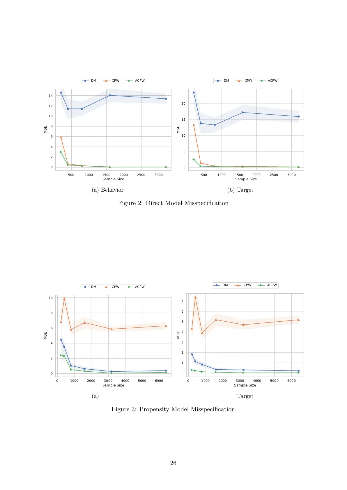
Bey ond Demand Estimation: Consumer Surplus Ev aluation via Cum ulativ e Prop ensit y W eigh ts Zeyu Bian ∗ † 1 , Max Biggs ‡ 2 , Ruijiang Gao § 3 , and Zhengling Qi ¶ 4 1 Florida State Univ ersity 2 Univ ersity of Virginia 3 Univ ersity of T exas at Dallas 4 George W ashington Univ ersit y Abstract This pap er develops a practical framework for using observ ational data to audit the consumer surplus eﬀects of AI-driv en decisions, speciﬁcally in targeted pricing and algorith- mic lending. T raditional approaches ﬁrst estimate demand functions and then in tegrate to compute consumer surplus, but these methods can b e challenging to implemen t in practice due to mo del missp eciﬁcation in parametric demand forms and the large data requirements and slow conv ergence of ﬂexible nonparametric or mac hine learning approac hes. Instead, w e exploit the randomness inheren t in mo dern algorithmic pricing, arising from the need to balance exploration and exploitation, and in tro duce an estimator that a v oids explicit estima- tion and n umerical in tegration of the demand function. Eac h observ ed purc hase outcome at a randomized price is an un biased estimate of demand and b y carefully rew eighting purc hase outcomes using no vel cumulativ e prop ensit y weigh ts (CPW), we are able to reconstruct the in tegral, or area under demand curv e, when these outcomes are aggregated. Building on this idea, we in tro duce a doubly robust v ariant named the augmented cum ulative prop en- sit y weigh ting (A CPW) estimator that only requires one of either the demand model or the historical pricing p olicy distribution to b e correctly sp eciﬁed. F urthermore, this approac h facilitates the use of ﬂexible machine learning methods for estimating consumer surplus, since it achiev es fast conv ergence rates b y incorp orating an estimate of demand, even when the machine learning estimate has slo wer con vergence rates. Neither of these estimators is a standard application of oﬀ-policy ev aluation tec hniques, since the target estimand, consumer surplus, is typically unobserved. T o address algorithmic fairness, w e extend this framework to an inequalit y-aw are surplus measure, allo wing regulators and ﬁrms to quantify the trade- oﬀ b et ween ﬁrm proﬁt and equit y . Finally , w e conduct a comprehensiv e numerical study to v alidate the theoretical prop erties of our prop osed metho ds. ∗ Alphab etical Order. † Email: zeyu.bian@fsu.edu ‡ Email: biggsm@darden.virginia.edu § Email: ruijiang.gao@utdallas.edu ¶ Email: qizhengling@email.gwu.edu 1 1 In tro duction With the proliferation of data on consumer b eha vior and the developmen t of sophisticated Artiﬁcial Intelligence (AI), ﬁrms are increasingly adopting autonomous, targeted algorithmic strategies to price go ods and oﬀer p ersonalized loans. F or example, many e-commerce ﬁrms will dynamically adjust prices based on an individual’s purc hasing history , demographics, or ev en bro wsing b eha vior (e.g., Hannak et al. ( 2014 )), while ﬁnancial ﬁrms employ similar targeted algorithms to set interest rates for auto loans, mortgages, and credit cards. Indeed, the setting of in terest rates is widely recognized as a form of targeted pricing, with recen t studies utilizing auto loan datasets to empirically demonstrate the eﬃcacy of algorithmic pricing strategies ( Ban and Keskin 2021 , Elmac htoub et al. 2023 , Miao et al. 2023 , Phillips et al. 2015 ). Although these prescriptiv e AI technologies promise to enhance mark et eﬃciency , b oost ﬁrms’ reven ues, and broaden inclusion through p ersonalized service, there are also concerns regarding their potential adv erse impact on consumers. A primary concern is that increased ﬁrm rev en ues due to targeted algorithms come at the exp ense of consumer surplus, with recen t mo dels from the academic literature suggesting that this burden can b e unfairly distributed ( Cohen et al. 2022 , Kallus and Zhou 2021a ). In addition, there is a gro wing c oncern that marginalized groups might b e disproportionately aﬀected by these pricing practices, facing steep er prices and lo w er surplus. F or example, ride-hailing services ha ve b een found to charge higher fares in neigh b orho ods with larger non-white p opulations and higher p o v erty lev els, indicating that these communities face larger price hik es due to algorithmic pricing strategies ( Pandey and Calisk an 2021 ). These concerns hav e drawn signiﬁcan t attention from policymakers and the media ( Flitter 2023 ). F or example, a White House rep ort ( White House 2015 ) highlighted the risks associated with algorithmic decision-making in pricing, the F ederal T rade Commission (FTC) recently initiated in vestigations in to p oten tial discriminatory pricing practices by mandating transparency from companies employing p ersonalized pricing sc hemes ( K&L Gates 2024 , Sisco 2024 ), and la wmak ers ha ve called for scrutin y of ma jor retailers’ pricing practices ( W arren and Casey 2024 ). Although there is signiﬁcan t in terest, it is not yet clear what the impact of more targeted algorithmic pricing policies will b e ( White House 2015 ). These developmen ts underscore the need for robust auditing to ols capable of ev aluating the impact of algorithmic pricing on consumer surplus and its distribution across customers. F or regulators lik e the FTC, suc h to ols can help ensure ﬁrms are abiding by relev ant laws and regulations, such as the Gender T ax Rep eal Act of 1995 (commonly known as the “Pink T ax”), whic h prohibits gender-based pricing discrimination ( Legislature 1995 ), or the Equal Credit Opp ortunit y Act (ECO A) that prohibits creditors from discriminating against demographic factors. They can also help p olicymak ers understand the impacts of v arious t yp es of algorithmic pricing and who is adversely aﬀected, leading to b etter guidelines and rules. Such to ols can also help ﬁrms assess regulatory or reputational risks of existing algorithms, and simulate outcomes to ensure future compliance. They also provide the opp ortunit y to strike a b etter balance b et w een short-term proﬁt and long-term customer relationships b y ensuring consumer surplus remains at sustainable lev els for all customer t yp es. Despite this need, there are issues regarding the eﬃcacy of existing consumer surplus es- timation metho ds. Typically , estimation tec hniques rely on ﬁrst estimating demand and then 2 in tegrating demand to calculate surplus (e.g., Bhattachary a ( 2024 )), so the accuracy of the surplus estimate is highly dependent on the accuracy of the demand estimate. This approach is inherently indirect and requires estimating demand as a p oten tially complex function of price, ev en when the surplus target can be a simple scalar. Classical demand mo dels depend on parametric assumptions ( Dagsvik and Karlstr¨ om 2005 , McF adden 1981 , Shiller et al. 2013 , Small and Rosen 1981a ) and can b e biased when b eha vior deviates from the assumed form ( Bhattac harya 2024 , Jagabathula and Rusmevic hientong 2017 ). More ﬂexible nonparametric and mac hine learning metho ds, suc h as neural netw orks ( F arrell et al. 2020 , 2021 ), relax func- tional assumptions but often require very large datasets and careful tuning to achiev e reliable accuracy , and typically ha v e slo wer con v ergence rates. Given these shortcomings, it is useful to explore more direct alternativ es for consumer surplus estimation that are less dep enden t on accurate demand estimation, and to in v estigate how to incorp orate mac hine learning estimates while still ac hieving fast con v ergence rates. One k ey feature of many successful mo dern pricing algorithms that can b e leveraged for new metho ds of surplus estimation is that they in v olve a degree of price exp erimen tation. In practice, market conditions, comp etitor actions, and consumer preferences ev olve ov er time, so pricing algorithms m ust contin uously explore the demand curve rather than solely exploit curren t prices to maintain optimality ( Besbes and Zeevi 2009 , Rana and Oliveira 2014 ). Recent empirical w ork ( Bray et al. 2024 ) has observed severe bias in the estimation of price sensitivity at a large sup ermarket c hain when using relatively static historic pricing data compared to exp erimen tal data, while Dub ´ e and Misra ( 2023 ) hav e demonstrated that prices set after a p erio d of price exp erimen tation drastically improv ed proﬁtabilit y at ZipRecruiter. These examples also indicate an increased willingness among ﬁrms to engage in exp erimen tation, which has b ecome more ubiquitous as e-commerce platforms enable con tinuous price up dates. While primarily in tended to supp ort proﬁt maximization, this inheren t randomization also provides a ric h source of quasi-exp erimen tal v ariation that can b e leveraged to estimate the consumer surplus. One natural approac h to utilizing such data and p otentially a voiding explicit demand es- timation is to adapt inv erse-prop ensit y-score w eighting (IPW) from causal inference ( Beygelz- imer and Langford 2009 , Rosen baum and Rubin 1983 ). How ev er, the a v ailabilit y of quasi- exp erimen tal data alone do es not solv e the fundamen tal diﬃculty of measuring consumer w el- fare. Unlik e rev enue, which is entirely determined by the price and the observed purchase decision, consumer surplus relies on the customer’s v aluation, a v ariable that is inherently la- ten t. In the observ ational data, we do not observe the surplus. Instead, we only observe a binary purchase decision, whic h serves as a coarse approximation indicating that the v aluation exceeded the price. Because the true outcome of in terest is never directly seen, standard causal inference techniques suc h as w eighting observ ed outcomes cannot b e directly applied. Motiv ated by these c hallenges, w e prop ose the new cumulativ e prop ensit y weigh t (CPW) estimator, which directly estimates consumer surplus and b ypasses the need for explicit demand mo deling. This approach leverages the randomness already present in the observ ational data due to the need to balance exploration and exploitation in many mo dern algorithmic pricing strategies. Intuitiv ely , eac h observ ed purchase outcome at a randomized price is an unbiased estimate of demand. By carefully reweigh ting that observ ation according to how often a target 3 pricing p olicy would oﬀer a price at or below the one observed for similar customers, relative to ho w frequen tly that price lev el app eared historically , we are able to reconstruct the consumer surplus, i.e., the integral or the area under the demand curve, when these weigh ted outcomes are aggregated. When the historical pricing p olicy is known or well do cumen ted, the approach is straightforw ard to implemen t and is entirely mo del-free. When it is unknown, the cumulativ e w eights can b e estimated from transaction data. Building on the cum ulativ e-weigh ts idea, w e in tro duce a doubly robust estimator with cross- ﬁtting that deliv ers reliable surplus estimates even when either the demand mo del or the his- torical pricing distribution is missp eciﬁed. Sp eciﬁcally , when the historical pricing p olicy is kno wn or can b e estimated accurately , consistency holds ev en with a biased demand mo del. In con trast, when demand is asymptotically unbiased, consistency holds even with a missp eciﬁed historical pricing mo del. F urthermore, mirroring standard doubly robust estimators in causal inference, our estimator achiev es eﬃciency under weak rate conditions without imp osing the Donsk er condition on either demand or cumulativ e-w eight estimation. This ﬂexibilit y enables the use of mo dern machine learning tec hniques and complex nonparametric mo dels. W e formally establish that our prop osed estimators are asymptotically equiv alent to the eﬃcient inﬂuence function, and therefore achiev e the low est p ossible asymptotic v ariance. Finally , w e pro ve the asymptotic normalit y of the proposed estimators, enabling the construction of v alid conﬁdence in terv als, enabling policymakers to assess the reliabilit y of these estimates. T o address fairness, we extend our ob jective from estimating the standard consumer surplus to estimating an inequality-a ware surplus. This new target captures b oth the magnitude of surplus a p olicy creates and its distribution across diﬀerent customer types via a single pre- sp eciﬁed parameter. At its baseline, this parameter replicates the standard arithmetic a v erage of customers’ surplus, but as it decreases, it places progressively greater weigh t on outcomes for worse-oﬀ groups. This approach is based on generalized mean aggregates as studied by Bergson ( 1954 ) and Atkinson et al. ( 1970 ). T o achiev e this ob jective, we derive the eﬃcient inﬂuence function of this new target and adapt our cumulativ e w eights approac h to construct an eﬃcient estimator. Due to the nonlinearit y of the ob jective, this estimator do es not inherit full double robustness. Instead, it is singly robust with resp ect to the demand mo del, in that consistency holds as long as the demand is correctly sp eciﬁed, ev en if the cumulativ e w eights are missp eciﬁed. This alters the theoretical requirements for establishing the asymptotic properties compared to the previous case: while incorp orating cumulativ e weigh ts still has the b eneﬁt of relaxed rate conditions, i.e., allowing ﬂexible mac hine learning mo dels, demand estimation requires stricter control, sp eciﬁcally satisfying standard nonparametric rates. Nevertheless, we deriv e v alid asymptotic prop erties for this new estimator and show it has the minimal asymptotic v ariance among all regular estimators, which enables auditors to rep ort v alid conﬁdence interv als for b oth aggregate and equit y-sensitive surplus. Our exp erimen ts conﬁrm the reliabilit y and robustness of the prop osed framew ork. F or the standard aggregate surplus, our doubly robust estimator accurately recov ers the true surplus ev en when either the demand or pricing mo del is missp eciﬁed, achieving the b est conv ergence rate when b oth are well sp eciﬁed. W e further ev aluate our inequality-a w are surplus, studying its estimation error and conﬁdence interv al cov erage. Despite the theoretical shift to single 4 robustness for this nonlinear ob jective, our results demonstrate that the estimator remains highly eﬀectiv e, pro ducing accurate point estimates and v alid conﬁdence in terv als across v arying equit y settings. T o further demonstrate the p o wer of this framework, we apply it to a large-scale ﬁnancial dataset of U.S. automobile loans. The global automotive market size was estimated at USD 2.75 trillion in 2025 and is pro jected to reach USD 3.26 trillion by 2030 ( Mordor In telligence 2025 ). It is an imp ortan t driv er of household ﬁnancial stabilit y and is increasingly dominated b y algorithmic underwriting. W e compare the welfare outcomes of a historical pricing p olicy against a trained AI pricing agen t. Our analysis reveals an aggregate consumer surplus–equit y tradeoﬀ: p ersonalized pricing reduces total consumer surplus while narro wing disparities across credit and p olitical groups, demonstrating the framework’s v alue for auditing and regulatory ev aluation. 2 Related W ork 2.1 Consumer Surplus Estimation There is a substantial literature on consumer surplus ev aluation in b oth discrete choice en viron- men ts, where consumers t ypically choose one alternativ e from a set (e.g., Bhattachary a ( 2015 ), McF adden ( 1972 ), Small and Rosen ( 1981b )), and con tinuous demand settings (e.g., Hausman ( 1981 ), Hausman and New ey ( 1995 , 2017 ), V artia ( 1983 )), such as gasoline purchases ( Poterba 2017 ). Our w ork is more closely aligned with discrete choice mo dels, but we fo cus on a single- item setting in whic h we observ e individual customer characteristics and a binary outcome indicating whether they purchase the item. Initially , parametric mo dels of demand were used for surplus estimation ( Dagsvik and Karlstr¨ om 2005 , Herriges and Kling 1999 , McF adden 1981 ), for example, the widely used logsum formula ( Small and Rosen 1981b ). This relies on strong assumptions about preferences and customer heterogeneit y , such as additiv e extreme-v alue error distributions, which ma y lead to misleading w elfare conclusions if the mo del is misspeciﬁed. T o o v ercome suc h restrictiv e assumptions and mak e inferences in a broader range of settings, man y semiparametric and nonparametric metho ds for estimating demand hav e b een developed ( Berry and Haile 2021 , Bhattachary a 2015 , Hausman and New ey 1995 , Matzkin 2016 ). These t ypically inv olv e ﬂexible nonparametric regression to ﬁt the demand function directly , follo wed b y an in tegration to calculate the surplus. F or example, in the contin uous setting, Hausman and Newey ( 1995 ) ﬁt demand using series and k ernel estimators, and use it to solv e a diﬀeren- tial equation based on Shephard’s Lemma. Subsequent research has fo cused on incorp orating unobserv ed consumer heterogeneit y into these mo dels ( Hausman and Newey 2016 , Lewb el and P endakur 2017 ). Similarly , in the discrete c hoice setting, Bhattachary a ( 2015 , 2018 ) estimates a conditional nonparametric probability of purchase for eac h item (demand in this setting), then in tegrates to estimate consumer surplus. Recent machine learning approac hes hav e used neural net works to ﬂexibly estimate demand and surplus with minimal functional-form assumptions ( F arrell et al. 2020 , 2021 ), including in discrete choice mo dels ( Aouad and D´ esir 2025 ). T ree ensem ble metho ds hav e also b een proposed ( Chen et al. 2019 , Chen and Mi ˇ si ´ c 2022 ). A com- prehensiv e accoun t of nonparametric consumer surplus estimation can b e found in Hausman 5 and Newey ( 2017 ) and Bhattachary a ( 2024 ). A critical trade-oﬀ in these nonparametric demand estimation metho ds is that conv ergence can b e slo wer, leading to worse ﬁnite-sample p erformance than in well-speciﬁed parametric mo dels. In either case, the consumer surplus estimates are only as accurate as the demand mo del. In contrast, we present approaches that do not require mo deling demand at all, and sho w that w e can achiev e faster conv ergence when w e ha ve a slowly conv erging demand model. Some recen t applications of consumer surplus estimation can b e found, for example, in Shiller et al. ( 2013 ), who use an ordered probit to analyze Netﬂix data. Dub´ e and Misra ( 2023 ) emplo y a Bay esian parametric framework to estimate surplus from a large-scale randomized price exp erimen t at ZipRecruiter. Other research has lev eraged quasi-exp erimen tal v ariation in prices. F or instance, Cohen et al. ( 2016 ) uses a regression discon tinuit y design to estimate price elasticities and surplus from Ub er’s surge pricing data. Muc h of this literature is fo cused on incorp orating income eﬀects, which is not the fo cus of our pap er. W e fo cus on settings where the exp enditure represen ts a small fraction of the consumer’s total budget. In such regimes, the income eﬀects are negligible, and the Marshallian consumer surplus pro vides a near-exact appro ximation of the Hic ksian compensating v ariation ( Willig 1976 ). Alternatively one can interpret our analysis as applying when consumer utilities are quasilinear. 2.2 Causal Inference and Oﬀ-P olicy Ev aluation Muc h of the recent work on auditing pricing algorithms can b e viewed through the lens of oﬀ-p olicy ev aluation (OPE). The OPE literature initially centered on the inv erse prop ensit y w eighting (IPW) framew ork: eac h observ ed outcome is weigh ted by the recipro cal of its treat- men t (in our setting, price) assignment probability , or prop ensit y score, yielding an unbiased estimate of the counterfactual rew ard when the prop ensity model is correct ( Beygelzimer and Langford 2009 , Rosen baum and Rubin 1983 ). A complementary line of research adv o cates the direct metho d (DM), whic h replaces missing coun terfactuals with ﬁtted v alues from an outcome mo del. When that mo del is correctly sp eciﬁed, the DM can b e more eﬃcien t than IPW ( Qian and Murphy 2011 , Shalit et al. 2017 ). Recognizing that either comp onent ma y b e missp eciﬁed in practice, the doubly-robust estimator ( Dud ´ ık et al. 2011 , Robins et al. 1994 , Zhou et al. 2023 ) blends the tw o ideas and remains consistent so long as either the prop ensit y mo del or the outcome mo del is estimated without systematic error. Empirical evidence suggests that, when at least one n uisance mo del is reasonably accurate, the doubly robust estimator ac hieves lo wer mean-squared error than either IPW or the DM on their own ( Dud ´ ık et al. 2014 ). The idea of the doubly robust metho d originates from the missing data literature ( Robins et al. 1994 , Tsiatis 2006 ) and has b een widely adopted in causal inference ( Bang and Robins 2005 , Cher- nozh uko v et al. 2018 , Hern´ an and Robins 2010 , Kennedy 2024 ) and policy learning/ev aluation ( Bian et al. 2023 , Kallus and Uehara 2020 , Liao et al. 2022 , Robins 2004 , Shi et al. 2018 , W allace and Mo o die 2015 , Zhou et al. 2023 ). In the management science communit y , there is a growing bo dy of literature that leverages oﬀ-p olicy learning techniques to estimate reven ue in pricing settings. This stream of researc h is often grounded in the “predictive to prescriptive” analytics framework ( Bertsimas and Kallus 6 2020 ), which formally in tegrates mac hine learning predictions with optimization mo dels to de- riv e decision policies from observ ational data. Complementing this methodological foundation, recen t studies ha ve dev elop ed rigorous statistical learning frameworks for p ersonalized reven ue managemen t ( Chen et al. 2022 , Kallus and Zhou 2018 ) and demonstrated the practical eﬃcacy of these data-driv en pricing algorithms through large-scale ﬁeld exp eriments ( F erreira et al. 2016 ). Sp eciﬁcally , researchers ha ve used OPE techniques to address pricing settings charac- terized by binary demand ( Biggs 2022 , Biggs et al. 2021 , Elmach toub et al. 2023 ), as well as censored demand resulting from inv en tory shortages ( Ban 2020 , Bu et al. 2022 , T ang et al. 2025 ), and unobserved confounding ( Kallus and Zhou 2021b , Miao et al. 2023 ). In contrast to these works, our primary ob jective is the estimation of consumer surplus rather than rev- en ue. This shift substantially alters the estimation problem: unlik e the standard OPE setting, where the outcome is directly observed, surplus relies on consumer v aluations that are never seen. In our con text, we observe only a binary purchase decision, a coarse pro xy indicating whether v aluation exceeds price rather than the contin uous v aluation itself. Because the true outcome v ariable is latent, con ven tional causal inference tec hniques cannot b e directly applied, necessitating the dev elopmen t of the nov el metho dological to ols presented here. 2.3 Organization The remainder of this pap er is organized as follows. Section 3 formalizes the consumer surplus estimation problem. Section 4 in tro duces the Cum ulativ e Prop ensit y W eigh ting (CPW) estima- tor, a no vel approac h that lev erages the randomness in algorithmic pricing to estimate surplus without explicit demand integration. Section 5 develops the Augmented CPW (ACPW) esti- mator, establishing its double robustness. Section 6 extends the framework to inequality-a w are surplus measures, in tro ducing a parameter to trade oﬀ aggregate surplus against equity . Sec- tion 7 pro vides the theoretical analysis, proving the asymptotic normalit y and eﬃciency of the prop osed estimators. Section 8 presents numerical exp erimen ts v alidating the metho d’s robust- ness and demonstrates its application to a large-scale U.S. auto loan dataset. Finally , Section 9 concludes with managerial implications. The app endices con tain pro ofs of all theorems and auxiliary lemmas. Lastly , w e pro vide an extension on partial iden tiﬁcation b ounds for settings where the o v erlap assumption is violated in App endix 10. 3 Problem F orm ulation Consider a p opulation of heterogeneous consumers with features X ∈ X , and v aluations (i.e., willingness to pay), V ∈ R + , in terested in purchasing at most one unit of an item. F or a ﬁxed price p , the av erage consumer surplus can b e deﬁned as the a verage excess of eac h consumer’s v aluation o ver the price they pa y , S ( p ) = E  ( V − p ) +  , where x + = max( x, 0). Alternatively , in a lending scenario, we can consider p as a p erio dic in terest paymen t and interpret V as the maximum interest the customer is willing to pay , 7 with the surplus b eing the p ositiv e diﬀerence b et w een them. Note, we may b e interested in assessing the conditional surplus S ( p | X ) = E V [( V − p ) + | X ] asso ciated with a particular group of in terest for comparison purposes, or p opulation surplus S ( p ) = E X E V [( V − p ) + | X ], which is the surplus ov er all customers. F or notational simplicity , we fo cus on the latter, but our results also hold for the former, unless otherwise noted. W e highligh t that this deﬁnition is consistent with traditional “area under the demand curve” calculation of consumer surplus ( Bhattachary a 2024 ), where the demand curve is deﬁned as the probability of purc hase, as highlighted in Section 3.1. W e do not incorp orate income eﬀects into the mo del and fo cus on go ods where exp enditure represents a small fraction of the consumer’s total budget. In this case, the income eﬀects are negligible ( Willig 1976 ). Alternatively , but resulting in the same framew ork, w e fo cus on customers with quasilinear utility . In general, ﬁrms are in terested in oﬀering and ev aluating pricing p olicies that can b e b oth targeted and sto c hastic, where the price oﬀered to the customer with feature X is asso ciated with a pricing p olicy π : X → ∆( P ), which is a conditional probabilit y mass/density o ver the price space P given the feature X ∈ X . Then the a verage consumer surplus under the pricing p olicy π is deﬁned as S ( π ) = E  Z P π ( p | X ) ( V − p ) + d p  , (1) where the underlying exp ectation is taken with resp ect to the join t distribution of ( X , V ). If V is observed, then one can estimate S ( π ) by directly using the sample av erage to approximate the exp ectation in Equation (1). How ev er, in practice, consumers’ v aluations V are typically unobserv ed, whic h presents a c hallenge for the estimation task. While a consumer’s v aluation V is often unobserved, typically their binary purc hase decision Y is often recorded at the price they were oﬀered P ∈ P . This purchase decision is determined by whether their v aluation exceeds the oﬀered price P : Y = I ( V > P ) . (2) where I ( · ) denotes the indicator function. Here, Y = 1 denotes a purchase (the condition is met), and Y = 0 denotes no purc hase. In addition to V b eing unobserved, we often face a distribution shift, where w e ma y w ant to ev aluate surplus under a pricing p olicy that is diﬀeren t from the historical p olicy that generated the data. In general, we consider three ob jectives: (i) ev aluating consumer surplus of a new pricing strategy (also referred as the target p olicy) π ; (ii) ev aluating the consumer surplus of a current or previously used pricing strategy π D from the historical data (also referred as the behavioral policy); and (iii) ev aluating the c hange in surplus b et w een historical and new policies: ∆( π ) = E  Z P ( π ( p | X ) − π D ( p | X )) ( V − p ) + d p  , (3) W e note that the historical pricing distribution π D ma y b e known or unkno wn, while π is alw ays kno wn. When the ﬁrm is engaged in algorithmic pricing, often the historical pricing p olicy is enco ded digitally and is therefore kno wn. When it is unkno wn, it can typically b e 8 estimated from the data. Generally , the diﬀerence b et w een ev aluating (i) and (ii) arises from unkno wn π D , which can in tro duce additional c hallenges in the estimation. W e will fo cus on this case when ev aluating (ii) unless otherwise noted. The oﬄine dataset can thus b e represen ted as ( X i , P i , Y i ) n i =1 , consisting of i.i.d. samples of ( X , P , Y ) generated under a historical pricing p olicy π D . Next, we present some conditions necessary for the iden tiﬁcation of the av erage consumer surplus S ( π ) under the observ ational data-ge nerating distribution. First, w e provide the formal deﬁnition of iden tiﬁcation. Deﬁnition 1 (Identiﬁabilit y) . A p ar ameter of inter est θ in a pr ob abilistic mo del {P θ : θ ∈ Θ } is said to b e identiﬁable if the mapping θ 7→ P θ is inje ctive, i.e., P θ 1 = P θ 2 = ⇒ θ 1 = θ 2 . F or identiﬁcation in this setting, w e require t wo conditions to hold: Assumption 1. (Ignor ability) P ⊥ ⊥ V | X . Assumption 2. (Overlap) The pric e data gener ating distribution satisﬁes π D ( p | x ) > 0 , for al l p ∈ P , and every x ∈ X . In addition, the supp ort P c ontains the supp ort of the valuation V . F or identifying ∆( π ) , we only r e quir e the supp ort of π D to c ontain the supp ort of π . Assumption 1 is similar to the classical causal assumptions of ignorabilit y or exchangeabilit y , see, e.g., Hern´ an and Robins ( 2010 ), Rosen baum and Rubin ( 1983 ). It states that, conditional on consumer c haracteristics X , the distribution of v aluations is unaﬀected b y the oﬀered price, facilitating the identiﬁcation of surplus. It is commonly satisﬁed as long as the factors that dro ve the historical pricing decisions are recorded and av ailable in the observed data. It is w orth noting that Assumption 1 do es not imp ose any parametric structure on the consumer v aluations model. Assumption 2 requires that ev ery p ossible price p ∈ P has a p ositiv e prob- abilit y of b eing observ ed for the observ ational data. This means the previous pricing p olicy m ust inv olv e some degree of randomization, which, as previously discussed, is necessary for a pricing p olicy to obtain and maintain optimalit y . Suc h a condition is similar to the p ositivit y condition in causal inference for identifying the av erage treatment eﬀect. Without this co ver- age assumption, nonparametric identiﬁcation of the demand function, and consequently , the absolute consumer surplus, is imp ossible without relying on strong extrap olation assumptions. Ho wev er, we note that the requirements are signiﬁcantly relaxed when ev aluating the diﬀerence in surplus b et w een tw o p olicies. In that context, we only require o verlap ov er the prices pro- p osed by the new p olicy π , rather than the en tire price space. While iden tifying absolute surplus requires observing demand at extreme prices (to capture total willingness to pay), estimating p olicy diﬀerences is often suﬃcient for decision-making and aligns with standard practices in the literature ( Bhattachary a 2024 ). While w e establish identiﬁcation and estimation results for b oth quan tities, w e ackno wledge the diﬀerence is easier to practically implement. T o address settings where Assumption 2 do es not hold, App endix 10 introduces an exten- sion that exploits demand function prop erties (sp eciﬁcally monotonicity and log-conca vity) to b ound the surplus. Exp erimental results in App endix 10.3 conﬁrm the v alidity of these partial iden tiﬁcation b ounds and illustrate their sup erior tightness compared to naiv e b ounds derived from the natural [0, 1] support of purchase probabilit y . 9 Next, we present a commonly used baseline approach for estimating S ( π ) and discuss its limitations. Without loss of generality , w e assume P = [0 , ∞ ). 3.1 Baseline Solution: Direct Metho d A classic approach to calculate the consumer surplus is to calculate the area under the demand curv e ab o v e a particular price (for example, Bhattachary a ( 2015 )). Under Assumption 1 w e sho w this form is equiv alen t to our consumer surplus deﬁnition (1) for the sto c hastic pricing p olicy setting S ( π ) = E  Z ∞ 0 π ( p | X ) Z ∞ z = p µ ( X , z ) dz dp  , (4) where µ ( x, z ) ≡ E [ Y | X = x, P = z ] ≡ P [ V > z | X = x ] is the probability of purchase, whic h can b e considered the demand function in this setting. A brief pro of showing the equiv alence is provided in Prop osition 3 in App endix 1.1 and follows from carefully changing the order of in tegration. While Assumption 2 is not strictly required for the deriv ation of this identit y , it is necessary for the iden tiﬁcation and estimation of µ ( x, z ) ov er the integration range. This equation shows that ev en when the v aluation V is unobserved, the surplus can still b e identiﬁed b y ﬁrst computing the integral of the demand function µ ( x, z ) ov er prices ab o ve p , and then taking a w eighted av erage o ver price using the target p olicy π . When surplus under the b eha vior p olicy π D , or the diﬀerence in surplus is of in terest, it simpliﬁes to S ( π D ) = E X,P ∼ π D  Z ∞ P µ ( X , z ) dz  , ∆( π ) = S ( π ) − S ( π D ) . (5) In practice, the demand function µ ( x, p ) is ge nerally unkno wn and must b e estimated by regressing Y on X and P , yielding an estimator b µ ( x, p ). Then the direct metho d (DM) uses the sample a v erage to appro ximate Equations (4) and (5) and gives b S DM ( π ) = 1 n n X i =1 Z ∞ 0 π ( p | X i ) Z ∞ p b µ ( X i , z ) dz dp, b S DM ( π D ) = 1 n n X i =1 Z ∞ P i b µ ( X i , z ) dz , (6) b ∆ DM ( π ) = b S DM ( π ) − b S DM ( π D ) , (7) where b µ ( · , · ) is the estimator of the demand function. W e note that the historic surplus esti- mator b S DM ( π D ) has the adv an tage of not requiring an estimate of the historic pricing p olicy distribution b π D (when it is unknown), compared to the naiv e approach of substituting b π D in to b S DM ( π ), highlighting the suitability of eac h estimator for its particular task. As discussed previously , the p erformance of the DM estimator dep ends critically on the accuracy of the outcome model b µ ( x, p ), which can be challenging to estimate in practice. T ra- ditional demand estimators that imp ose ﬁxed parametric forms can yield biased results when- ev er actual purchasing b eha vior stra ys from those assumptions. In contrast, modern fully non-parametric tec hniques, such as neural-net work demand mo dels ( F arrell et al. 2020 , 2021 ), a void functional-form missp eciﬁcation but generally require a very large sample b efore they de- liv er reliable accuracy , limiting their practicality in man y observ ational settings. F urthermore, 10 the DM relies on n umerical in tegration of estimated functions. This step requires the underlying estimation to b e uniformly accurate across P . Lastly , the n umerical integration pro cedure itself can introduce bias and raise computational burden since the integration m ust o ccur ov er all prices for ev ery datap oin t. These limitations asso ciated with the DM estimator motiv ate the exploration of alternative approac hes. In the next section, we present our newly prop osed solutions for identifying and estimating S ( π ). 4 Cum ulativ e Prop ensit y W eigh ts Represen tation and Estima- tion W e next present an alternative approac h for consumer surplus estimation that a v oids the chal- lenges of estimating a demand function and n umerical integration. This estimator leverages the price v ariation already present in mo dern algorithmic pricing due to the need to balance explo- ration and exploitation. Rather than explicitly integrating to get the area under an estimated demand curve, the estimator appro ximates this area by an aggregate of weigh ted purchase out- comes, each of whic h is an unbiased estimate of demand at a giv en price. By carefully w eighing the observ ations, we can recov er the consumer surplus in exp ectation. F ormally , our estimator is motiv ated by the following alternativ e identiﬁcation result. Theorem 1. Under Assumptions 1 and 2, we have S ( π ) = E  F π ( P | X ) π D ( P | X ) Y  , (8) wher e F π ( p | x ) denotes the cumulative distribution fu nction under the tar get p olicy, i.e., F π ( p | x ) ≡ R p 0 π ( u | x ) du . Pr o of. The pro of follows from the law of iterated exp ectations and a change of the order of in tegration: E  Z ∞ p =0 π ( p | X ) Z ∞ z = p µ ( X , z ) dz dp  | {z } Equation (4) = E  Z ∞ p =0 Z ∞ z = p π ( p | X ) µ ( X , z ) dz dp  = E  Z ∞ z =0 Z z p =0 π ( p | X ) µ ( X , z ) dp dz  = E  Z ∞ z =0  Z z p =0 π ( p | X ) dp  µ ( X , z ) dz  = E  Z ∞ z =0 F π ( z | X ) π D ( z | X ) µ ( X , z ) π D ( z | X ) dz  = E  F π ( P | X ) π D ( P | X ) Y  . Analogously , the historical consumer surplus and c hange in surplus can b e identiﬁed by replacing π with π D in Equation (8) and taking the diﬀerence: S ( π D ) = E  F π D ( P | X ) π D ( P | X ) Y  , and ∆( π D ) = E  ( F π ( P | X ) − F π D ( P | X )) π D ( P | X ) Y  . (9) 11 0 0 . 2 0 . 4 0 . 6 0 . 8 1 p 1 p 2 p 3 p ′ 1 p ′ 2 p ′ 3 p ′ 4 p ′ 5 p ′ 6 p ′ 7 p ′ 8 p ′ 9 p ′ 10 p ′ 11 p ′ 12 p ′ 13 E [ Y | P = z ] Exp ected Demand Demand for T arget p i Demand for Observ ed p ′ i Surplus from p i 0 0 . 1 0 . 2 0 . 3 0 . 4 0 . 5 0 . 6 0 . 7 0 . 8 0 . 9 1 0 0 . 2 0 . 4 0 . 6 0 . 8 1 z (price) CDF of target p olicy Figure 1: Illustrative example highlighting the cumulativ e prop ensit y weigh ts and their rela- tionship to the area under the demand curve. See Example 1 for more details. Based on Theorem 1, our prop osed CPW estimators can b e derived b y taking the sample a verage of Equation (8): b S C P W ( π ) = 1 n n X i =1 F π ( P i | X i ) b π D ( P i | X i ) Y i , b S C P W ( π D ) = 1 n n X i =1 b F π D ( P i | X i ) b π D ( P i | X i ) Y i , (10) b ∆ C P W ( π ) = 1 n n X i =1 ( F π ( P i | X i ) − b F π D ( P i | X i )) b π D ( P i | X i ) Y i , (11) where b π D and b F π D are the estimators for the density and cumulativ e density for the historic p olicy , resp ectiv ely . W e next presen t a simple example, illustrated in Figure 1, to give further in tuition b ehind the CPW estimator. Example 1. Supp ose that we ar e estimating the c onsumer surplus for a tar get-pricing p olicy that assigns e qual pr ob ability to thr e e discr ete pric es p 1 < p 2 < p 3 , with the c orr esp onding exp e cte d demand shown in gr e en cir cles. Assume the c ontext is the same for al l customers. The c onsumer surplus under this tar get p olicy c an b e r epr esente d as a sc aling of the aver- age of the thr e e ar e as to the right of the p olicy pric es under the demand curve: S ( π ) = E h R ∞ 0 π ( p | X ) R ∞ z = p µ ( X , z ) dz dp i = 1 3 P 3 i =1 1 3 R ∞ z = p i E [ Y | P = z ] dz . In Figur e 1 these ar e the thr e e pink r e gions. Wher e they overlap the tint is darker, r eﬂe cting the fact that the ar e a to the right of p 3 is c ounte d in all three inte gr als, the r e gion b etwe en p 2 and p 3 is c ounte d in t wo , and 12 the r e gion b etwe en p 1 and p 2 is c ounte d in one . Now assume that the historic al data wer e gener ate d by a (known) historic al pricing p olicy, uniformly distribute d fr om 0 to 1. In the historic al data, we happ en to observe 13 r andom r e alize d pric es { p ′ i } 13 i =1 , which is a sp arse r epr esentation of what would o c cur with mor e samples. Each r e alize d p air ( p ′ i , Y i ) gives an unbiase d snapshot of exp e cte d demand at that thr eshold, i.e., E [ Y | P = p ′ i ] , wher e the black cir cles indic ate the c onditional exp e ctations to which empiric al aver ages c onver ge with suﬃcient data for e ach pric e p oint. If we wer e to aggr e gate the outc omes Y i (or exp e cte d outc omes with enough data), we would appr oximate the total ar e a under the demand curve. However, to appr oximate the c onsumer surplus for the tar get pricing p olicy by aggr e gation, we ne e d diﬀer ent weights. In p articular, to r e cr e ate the pr evious surplus c alculation, we must weight observations at p ′ 11 , p ′ 12 , p ′ 13 by thr e e times as much as at p ′ 5 , p ′ 6 , p ′ 7 , p ′ 8 , sinc e the ar e a under the curve in [ p 3 , 1) is include d in the surplus c alculation for al l thr e e pric es under the tar get p olicy (dark pink), wher e as [ p 1 , p 2 ) is only include d onc e (light pink). [0 , p 1 ) is not include d at al l, while [ p 2 , p 3 ) is include d twic e. This weight is the fr action of tar get p olicy pric es whose surplus includes that historic al pric e and is pr op ortional to the cumulative tar get mass, which for the thr e e-p oint tar get p olicy is F π ( p ′ i ) = 1 3 P 3 j =1 1 { p ′ i ≥ p j } (i.e., F π ( p ′ 1 ) = 0 , F π ( p ′ 5 ) = 1 / 3 , F π ( p ′ 9 ) = 2 / 3 , F π ( p ′ 11 ) = 1 ). This is shown in the lower p anel of Figur e 1. As a r esult, with mor e sample d pric e p oints along the r ange of pric es, the weighte d aver age 1 n P n i =1 F π ( p ′ i ) π D ( p ′ i ) Y i wil l eventual ly appr oximate the ar e a under the demand curve, weighte d by the fr e quency it is include d in the tar get surplus c alculation, i.e., 1 3 P 3 i =1 π ( p i ) R ∞ z = p i E [ Y | P = z ] dz , as the numb er of samples gets lar ge. 1 This approach contrasts with standard IPW in oﬀ-p olicy ev aluation in t wo signiﬁcan t w ays. First, the observ able Y is not the unobserved surplus, ( V − P ) + , we are trying to estimate under the new pricing p olicy . Second, the numerator of the weigh ting term is the cumulativ e target p olicy densit y F π ( P | X ), not the target density π ( P | X ) at P that t ypically app ears in IPW. This is due to the need to estimate the av erage of an integral (or area) rather than the usual av erage outcome. As such, standard IPW tec hniques cannot be applied. Compared to the direct metho d (Equation (4)), this result requires knowledge, or an esti- mate, of the pricing distribution π D instead of the demand function µ ( X , P ). When the historic pricing p olicy is kno wn, this estimator is un biased and completely mo del-free. This ma y o ccur if a company is in v estigating the consumer surplus implications of its o wn algorithmic pricing p olicy , or a p olicymak er mandates that the algorithm b e made av ailable for audit. Alterna- tiv ely , if the historical pricing p olicy is relatively simple, it may b e muc h easier to estimate than a complex demand function. F urthermore, the DM requires numerical in tegration ov er the price space P for every observ ation, whic h can b e computationally exp ensive. In contrast, the CPW estimator is a simple w eighted av erage, making it computationally eﬃcien t for large datasets. This alternative estimator provides the regulator or ﬁrm with crucial ﬂexibility in surplus estimation. Nev ertheless, the p erformance of the CPW estimator remains sensitive to the accuracy of the estimated historical pricing p olicy distribution when it is not a v ailable and ma y b e sub ject 1 In this case, the historic pricing p olicy is uniform, π ( p ′ i ) = 1, so the denominator do es not impact the calculation, but would otherwise be the usual inv erse prop ensity correction to make the historical p olicy as if it w ere uniform in exp ectation. 13 to missp eciﬁcation. T o further address this issue, we in tro duce the augmen ted CPW (ACPW) estimator, whic h com bines elemen ts of both the DM and CPW approac hes, remaining consistent if either component is correctly speciﬁed, and is therefore more robust. 5 Doubly Robust Represen tation and Estimation The construction of the ACPW estimator is grounded in the theory of the eﬃcien t inﬂuence function (EIF). The EIF is piv otal for tw o main reasons: it characterizes the semiparametric eﬃciency b ound (the minimal asymptotic v ariance of any regular estimator), and it pro vides a constructiv e mec hanism for ac hieving this b ound. Intuitiv ely , the EIF acts as a correction term that remo ves the ﬁrst-order bias from a naive plug-in estimator (e.g., DM or CPW estimators in our context). This correction is essen tial for ensuring that the ﬁnal estimator remains √ n - consisten t and asymptotically normal, ev en when the nuisance components (such as the demand function and cum ulative w eights) conv erge at slo wer rates. F ormally , the EIF is deﬁned as the canonical gradient of the target parameter, e.g., S ( π ), S ( π D ) and ∆( π ), with resp ect to the underlying data distribution. By constructing our estimator based on this gradien t, w e ensure it is asymptotically eﬃcient (i.e., minimax optimal). F or a comprehensive treatment of this theory , we refer readers to Tsiatis ( 2006 ). W e no w presen t the deriv ed EIF for S ( π ) under our semi-parametric mo del (2). Let D = ( X , P , Y ). Theorem 2. Supp ose Assumptions 1 and 2 hold, the EIF for S ( π ) is ψ π ( D ) = Z ∞ 0 π ( p | X ) Z ∞ p µ ( X , z ) dz dp + F π ( P | X ) π D ( P | X ) ( Y − µ ( X , P )) − S ( π ) . (12) If the b ehavior p olicy π D is evaluate d, then the EIF takes the form ψ π D ( D ) = Z ∞ P µ ( X , z ) dz + F π D ( P | X ) π D ( P | X ) ( Y − µ ( X , P )) − S ( π D ) . (13) Final ly, the EIF for the diﬀer enc e in surplus ∆( π ) is given as ψ ∆ ( D ) = ψ π ( D ) − ψ π D ( D ) . This is formally prov ed in Appendix 2. A key prop erty of the EIF is that it has mean zero. This motiv ates the follo wing estimators, deﬁned by setting the empirical mean of the EIFs in Equations (12) and (13) to zero: e S AC P W ( π ) = 1 n n X i =1  Z ∞ 0 π ( p | X i ) Z ∞ p b µ ( X i , z ) dz dp + F π ( P i | X i ) b π D ( P i | X i ) ( Y i − b µ ( X i , P i ))  , (14) e S AC P W ( b π D ) = 1 n n X i =1  Z ∞ P i b µ ( X i , z ) dz + b F π D ( P i | X i ) b π D ( P i | X i ) ( Y i − b µ ( X i , P i ))  , (15) e ∆ AC P W ( π ) = e S AC P W ( π ) − e S AC P W ( b π D ) . (16) One can observe that the A CPW estimator integrates elements of b oth the DM and CPW approac hes, and it can b e shown that the ACPW estimator remains consistent if either the demand function or the b eha vior p olicy is correctly sp eciﬁed, a prop ert y known as double 14 robustness. The double robustness property is formally stated in the follo wing prop osition for the case of the known target p olicy , but the other cases also hold with near iden tical proofs. Prop osition 1. L et ¯ µ ( x, p ) and ¯ π D ( p | x ) denote the p opulation limits of the estimators b µ ( x, p ) and b π D ( p | x ) , r esp e ctively, such that: sup x,p | b µ ( x, p ) − ¯ µ ( x, p ) | = o p (1) and sup x,p | b π D ( p | x ) − ¯ π D ( p | x ) | = o p (1) . If either of the fol lowing c onditions holds: (i) ¯ µ ( X , P ) = µ ( X , P ) , almost sur ely; (ii) ¯ π D ( P | X ) = π D ( P | X ) , almost sur ely. Then we have c onsistency such that:    e S AC P W ( π ) − S ( π )    = o p (1) , wher e o p (1) denotes a quantity that c onver ges to zer o in pr ob ability as the sample size n → ∞ . The pro of of Prop osition 1 can b e found in App endix 3. This prop erty is imp ortan t b ecause it provides the regulator with ﬂexibility in surplus estimation, dep ending on whether consistent demand estimation or historical pricing p olicy density estimation is p ossible to ac hieve. Besides the desirable doubly robust prop ert y , another adv an tage of the ACPW estimator is that, under minimal rate conditions on the tw o nuisance estimators (the demand function and the b ehavior p olicy density), it can achiev e the low est p ossible v ariance b ound when combined with data splitting or a cross-ﬁtting pro cedure ( Chernozh uko v et al. 2018 ). W e next outline the K -fold cross-ﬁtting pro cedure, a minor algorithmic mo diﬁcation of the v anilla ACPW estimators in Equations (14) and (15). Sp eciﬁcally , we partition the sample indices { 1 , . . . , n } into K disjoint folds of appro ximately equal size, with any ﬁnite n umber K . F or each observ ation i , let k ( i ) denote the fold containing i . Denote b y b µ − k ( i ) ( x, p ) and b π − k ( i ) D ( p | x ) the estimators of the demand function and the b eha vior p olicy , resp ectively , which are trained using only the data excluding the k ( i )-th fold (hence the notation − k ( i )). The resulting A CPW estimator with cross-ﬁtting is denoted as b S AC P W ( π ) = 1 n n X i =1 " Z ∞ 0 π ( p | X i ) Z ∞ p b µ − k ( i ) ( X i , z ) dz dp + F π ( P i | X i ) b π − k ( i ) D ( P i | X i ) ( Y i − b µ − k ( i ) ( X i , P i )) # , b S AC P W ( π ) = 1 n n X i =1 " Z ∞ 0 π ( p | X i ) Z ∞ p b µ − k ( i ) ( X i , z ) dz dp + F b π D , − k ( i ) ( P i | X i ) b π − k ( i ) D ( P i | X i ) ( Y i − b µ − k ( i ) ( X i , P i )) # . This cross-ﬁtting approac h ensures that each observ ation is ev aluated using nuisance estimates ﬁtted on indep enden t data, thereb y reducing o verﬁtting bias and enabling v alid asymptotic inference even when the nuisance functions are estimated by ﬂexible machine learning metho ds, as will be detailed in Section 7. 6 Inequalit y-Aw are Surplus A common concern among p olicymakers when ev aluating a pricing p olicy is not only how the aggregate surplus c hanges, but also how it is distributed among consumers. In particular, there are concerns ab out equit y and the impact on those who are worst oﬀ. One approach used 15 in welfare economics to address these issues is to emphasize outcomes for customers with the lo west surplus when aggregating surpluses across the p opulation. W e follo w this direction by extending the prop osed oﬀ-p olicy consumer surplus estimation tec hniques to w elfare measures that are sensitiv e to ho w surplus is distributed across customer types. Let S ( π | X ) denote the surplus for customers with characteristics X , which represent customer t yp es. Earlier sections implicitly aggregated w elfare using the arithmetic mean, S ( π ) = E X [ S ( π | X )], eﬀectively av eraging across all customer types. F ollo wing the Atkin- son tradition and related w ork ( A tkinson et al. 1970 , Bergson 1954 , Dub´ e and Misra 2023 , Lewb el and Pendakur 2017 ), we instead consider the generalized-mean family ( S r ( π )) 1 /r , (17) where S r ( π ) := E X  S ( π | X ) r  . This coincides with the standard arithmetic av erage when r = 1 and increasingly prioritizes low er-surplus groups as r decreases, b ecoming more inequalit y a verse. This supplies a transparent p olicy parameter r that trades oﬀ aggregate surplus against its dispersion across customer segmen ts. The contin uous extension at r = 0 yields the geometric mean, and r = − 1 yields the harmonic mean. In the follo wing, for brevity , we fo cus on r  = 0 to a void restating results that are functionally the same. F or a ﬁnite sample { X i } n i =1 , the standard DM estimator is: 1 n n X i =1 b S ( π | X i ) r ! 1 /r = " 1 n n X i =1  Z ∞ 0 π ( p | X i ) Z ∞ p b µ ( X i , z ) dz dp  r # 1 /r , (18) Without loss of generality , we will fo cus on estimating S r ( π ), whic h can b e transformed after estimation to recov er S r ( π ) 1 /r . Next, w e derive the eﬃcient inﬂuence function for the target S r ( π ) and b eha vioral S r ( π D ) p olicies and their corresp onding eﬃcien t estimators. The EIF is giv en by the following theorem. Theorem 3. Under Assumptions 1 and 2, for r  = 0 , the EIF for S r ( π ) is r ( Y − µ ( X , P )) F π ( P | X ) π D ( P | X )  Z ∞ 0 π ( p | X ) Z ∞ p µ ( X , z ) dz dp  r − 1 +  Z ∞ 0 π ( p | X ) Z ∞ p µ ( X , z ) dz dp  r − S r ( π ) , (19) and the EIF for S r ( π D ) is r  ( Y − µ ( X , P )) F π D ( P | X ) π D ( P | X ) + Z ∞ P µ ( X , z ) dz   Z ∞ 0 π D ( p | X ) Z ∞ p µ ( X , z ) dz dp  r − 1 +(1 − r )  Z ∞ 0 π D ( p | X ) Z ∞ p µ ( X , z ) dz dp  r − S r ( π D ) . (20) By line arity, the EIF of ∆ r ( π ) fol lows by taking the diﬀer enc e b etwe en the ab ove two EIFs. Theorem 3 establishes the EIF for the inequalit y-aw are surpluses, S r ( π ), S r ( π D ) and their diﬀerence ∆ r ( π ) and is pro ved in App endix 4. In more detail, Equation (19) shares a structure 16 analogous to the EIF for the standard surplus in Equation (12): the R ∞ 0 π ( p | X ) R ∞ p µ ( X , z ) dz dp term corresp onds to the DM component, while ( Y − µ ( X ,P )) F π ( P | X ) π D ( P | X ) is a mean-zero de-biasing term incorp orating cumulativ e weigh ts, whic h plays a crucial role in v ariance reduction, enabling the resulting estimator to attain the semiparametric eﬃciency b ound. Naturally , Theorem 3 motiv ates the follo wing estimators to estimate S r ( π ) and S r ( π D ) resp ectiv ely , obtained by setting the empirical mean of the EIF to zero together with cross-ﬁtting: b S r ( π ) = 1 n n X i =1 " r ( Y i − b µ − k ( i ) ( X i , P i )) F π ( P i | X i ) b π − k ( i ) D ( P i | X i )  Z ∞ 0 π ( p | X i ) Z ∞ p b µ − k ( i ) ( X i , z ) dz dp  r − 1 +  Z ∞ 0 π ( p | X i ) Z ∞ p b µ − k ( i ) ( X i , z ) dz dp  r # , (21) b S r ( π D ) = 1 n n X i =1 " r ( Y i − b µ − k ( i ) ( X i , P i )) b F π D , − k ( i ) ( P i | X i ) b π − k ( i ) D ( P i | X i ) + Z ∞ P i b µ − k ( i ) ( X i , z ) dz ! ×  Z ∞ 0 b π − k ( i ) D ( p | X i ) Z ∞ p b µ − k ( i ) ( X i , z ) dz dp  r − 1 + (1 − r )  Z ∞ 0 b π − k ( i ) D ( p | X i ) Z ∞ p b µ − k ( i ) ( X i , z ) dz dp  r # Then b ∆ r ( π ) = b S r ( π ) − b S r ( π D ). W e refer to this class of estimators as the inequality-a w are ACPW estimator (IA-ACPW). Although the estimator b S r ( π ) in Equation (21) is deriv ed from the EIF in (19) and incorporates b oth DM and CPW elements, it do es not p ossess the double robustness prop ert y typically asso ciated with the A CPW estimator. This stems from the fact that the functional S r ( π ) is nonlinear when r  = 1. F or example, the functional reweigh ts observ ations such that small surpluses gain more lev erage for r < 1. Consequently , a single data p oin t perturbs the estimator diﬀeren tly than it would under a simple arithmetic mean. Due to this nonlinearity , b S r ( π ) is consisten t only if the demand mo del is correctly sp eciﬁed, although the historic pricing policy b π D can b e missp eciﬁed. The necessity of consistency for the demand estimation can clearly b e seen in Equation (21), where the ﬁrst term disapp ears when 1 n P n i =1  Y i − b µ − k ( i ) ( X i , P i )  con verges to 0, leaving the second term whic h is clearly only consisten t when demand is consisten t. How ev er, as we will sho w in the asymptotic analysis in Section (7.2), the cumulativ e weigh ts pla y an imp ortan t role in reducing v ariance, enabling the use of ﬂexible mac hine learning p olicies with slo wer con vergence rates. The estimation of the inequality-a w are surplus of the b eha vioral p olicy S r ( π D ) presents an even greater c hallenge. Unlik e b S r ( π ), the estimator b S r ( π D ) do es not enjoy even single robustness; it requires the simultaneous consistency of b oth the demand mo del b µ and the prop ensit y mo del b π D . This added fragility arises because π D is not kno wn but estimated, and it serv es a dual role: it acts as the prop ensit y w eigh t in the debiasing term and explicitly deﬁnes the integration measure in the demand term. Consequen tly , if b π D is missp eciﬁed, the estimator con verges to a functional of the wrong policy , preven ting consistency ev en if the demand mo del 17 b µ is p erfect. An example sho wing inconsistency of b S r ( π ) with a missp eciﬁed demand mo del is giv en next. Example 2. (Ine quality-awar e ACPW estimator is not r obust to demand missp e ciﬁc ation) Con- sider estimating the functional S r ( π ) =  Z ∞ 0 π ( p ) Z ∞ z = p µ ( z ) dz dp  r with r = 1 2 , in a setting without c ovariates, wher e µ ( · ) ≡ E [ Y | P = · ] denotes the demand function. Assume P ∼ Uniform[0 , 1] , so the b ehavior p olicy satisﬁes π D ( p ) = 1 for al l p ∈ [0 , 1] . L et the tar get p olicy also b e π ( p ) = 1 , which implies F π ( z ) = z , and supp ose the true demand function is µ ( p ) = 1 − p 2 . Under this setup, deﬁne θ ∗ = Z 1 0 π ( p ) Z 1 p µ ( z ) dz dp = Z 1 0 1 ·  z − z 3 3  1 p dp = Z 1 0  2 3 − p + p 3 3  dp = 1 4 , so that S r ( π ) = ( θ ∗ ) 1 / 2 = 1 2 . Now, supp ose the analyst uses a missp e ciﬁe d line ar demand mo del whose limiting ﬁt is ¯ µ ( p ) = 1 − 1 2 p. The c orr esp onding ﬁrst-stage limit is ¯ θ = Z 1 0 π ( p ) Z 1 p ¯ µ ( z ) dz dp = Z 1 0 1 ·  z − z 2 4  1 p dp = Z 1 0  3 4 − p + p 2 4  dp = 1 3 . Henc e, the p opulation limit of the IA-ACPW estimator is ¯ θ 1 / 2 + 1 2 ¯ θ − 1 / 2 E  F π ( P ) π D ( P )  Y − ¯ µ ( P )   | {z } R 1 0 z (0 . 5 z − z 2 ) dz = − 1 / 12 = r 1 3 − √ 3 24 , which diﬀers fr om the true value 1 / 2 . Ther efor e, even when the b ehavior p olicy is c orr e ctly sp e ciﬁe d, missp e ciﬁc ation of the demand mo del c ombine d with the nonline arity of the tar get functional yields a non-vanishing se c ond-or der r emainder term and le ads to bias. 7 Theoretical Analysis In this section, we establish the asymptotic normality of our prop osed estimators and highligh t the conditions required to achiev e this. These results are particularly imp ortan t, since they enable statistical inference and the construction of conﬁdence interv als for surplus estimates. In practice, this allows ﬁrms to rigorously assess whether c hanges in their pricing strategy lead to statistically signiﬁcan t improv emen ts in ov erall surplus or consumer welfare. F or example, an e- commerce company ma y wish to ev aluate whether a newly deplo yed dynamic pricing algorithm π yields a higher expected consumer surplus than the existing pricing strategy π D . By constructing conﬁdence in terv als for the respective estimators, the ﬁrm can formally test whether the observ ed impro vemen t is statistically meaningful, rather than the result of random v ariation in sales data. W e also show that these estimators attain the semiparametric eﬃciency b ounds. This means 18 that, among all regular and asymptotically linear estimators, our prop osed estimators achiev e the low est p ossible asymptotic v ariance. Although all estimators for the same target achiev e this b ound, the assumptions required to ac hiev e it can diﬀer, and in particular we sho w that the conditions for ACPW are relativ ely mild, allo wing fast rates of con vergence even if the demand function or historical price density estimates conv erge at slow er rates. Throughout, w e assume that all deriv ed EIFs hav e ﬁnite second moments, b π D ( p | x ) > c for some constant c , and that b µ ( x, p ) is bounded for all p and x . In what follows, w e start with the standard consumer surplus ( r = 1), where the strongest results can b e established, b efore progressing to the inequalit y-aw are surplus, which presents additional c hallenges. W e focus on analyzing the estimators for the surplus of a known p olicy π . Analogous results for the b eha vior p olicy surplus S ( π D ) and diﬀerence ∆( π ) follo w similar tec hniques and can b e found in App endix 6. F or completeness, we additionally present the results for the DM metho d, which forms part of our theoretical con tribution. 7.1 Analysis of Standard Consumer Surplus ( r = 1) W e impose three sets of technical conditions corresp onding to three estimators: CPW, A CPW, and DM, although we co ver assumptions for DM in App endix 5.1 for brevity . W e b egin with the assumptions required for the CPW estimator. 7.1.1 Required Assumptions Assumption 3 (Assumptions required for the CPW) . (i) q E [ b ω ( X , P ) − ω ( X , P )] 2 = o p (1) , wher e ω ( x, p ) ≡ F π ( p | x ) π D ( p | x ) , and b ω ( x, p ) ≡ F π ( p | x ) b π D ( p | x ) is the estimator of ω ( x, p ) . (ii) The b ehavior p olicy is estimate d using a function class that satisﬁes the Donsker pr op erty. (iii) Ther e exist b asis functions ϕ ( x, p ) ∈ R L and a ve ctor β ∈ R L such that sup x,p | µ ( x, p ) − ϕ ( x, p ) ⊤ β | = O ( L − s/d ) , (22) wher e s is a ﬁxe d p ositive c onstant and O ( · ) is the standar d big- O term. (iv) The estimate d CPW weights satisfy      1 n n X i =1 ϕ π ( X i ) − 1 n n X i =1 b ω ( X i , P i ) ϕ ( X i , P i )      2 = o p ( n − 1 / 2 ) , wher e ∥ · ∥ 2 is denote d as Euclide an norm, ϕ ( · , · ) is the b asis function that satisfy Equation (22) , and ϕ π ( x ) = R ∞ 0 π ( p | x ) R p ϕ ( x, z ) dz dp . Assumption 3 (i) is relativ ely mild, as it merely requires b π D to b e consistent, with no rate sp eciﬁed. Assumption 3 (ii) imp oses a complexity (size) constraint on the function class used for estimating the b eha vior policy . Before further discussing this assumption, w e formally deﬁne the Donsker class as follo ws. Deﬁnition 2 ( P -Donsker Class) . L et ( X , A , P ) b e a pr ob ability sp ac e and F b e a class of me asur able functions. We denote by L 2 ( P ) the sp ac e of al l me asur able functions that ar e squar e- 19 inte gr able with r esp e ct to P . The asso ciate d L 2 -norm is deﬁne d as ∥·∥ P, 2 . We deﬁne the fol lowing c omp onents to char acterize the c omplexity of F : • Br ackets: for any two functions l , u ∈ L 2 ( P ) , the br acket [ l , u ] is the set of functions { f : l ( x ) ≤ f ( x ) ≤ u ( x ) for al l x ∈ X } . An ϵ -br acket in L 2 ( P ) is a br acket [ l, u ] such that ∥ u − l ∥ P, 2 < ϵ . • Br acketing numb er: the br acketing numb er N [] ( ϵ, F , L 2 ( P )) is the minimum numb er of ϵ -br ackets in L 2 ( P ) ne e de d to c over F . • Br acketing inte gr al: the entr opy inte gr al is deﬁne d as J [] ( δ, F , L 2 ( P )) = Z δ 0 q log N [] ( ϵ, F , L 2 ( P )) dϵ Assume that ther e exists a me asur able function F such that | f ( x ) | ≤ F ( x ) for al l f ∈ F and x ∈ X , with E ( F 2 ) < ∞ . Then the class F is c al le d a P -Donsker class if J [] ( δ, F , L 2 ( P )) < ∞ , for some δ > 0 . In tuitively sp eaking, a Donsker class is a collection of functions that is not to o large or to o complex. This helps ensure that the a verage b eha vior of these functions b ecomes stable as w e collect more data. Many commonly used machine learning mo dels form Donsk er classes. These include standard parametric mo dels suc h as linear and generalized linear mo dels, as well as nonparametric regression metho ds like wa v elets and tensor pro duct B-splines (see Section 6 of Chen and Christensen ( 2015 ) for a review). How ev er, it is imp ortant to note that man y mo dern blac k-b o x machine learning algorithms do not inherently satisfy the Donsker prop ert y . High- capacit y mo dels, suc h as o ver-parameterized deep neural net works, unpruned random forests, or gradien t b o osting mac hines, often op erate in function spaces with massive complexit y . Without explicit structural constrain ts (e.g., sparsity , norm regularization, or b ounded depth), these classes can b e to o rich to admit a uniform Central Limit Theorem. Nevertheless, under sp eciﬁc tec hnical conditions, even these state-of-the-art mo dels can b e shown to satisfy the Donsker prop ert y . F or instance, Breiman et al. ( 2017 ) discusses conditions for decision trees, while Zhou et al. ( 2023 ) (Lemma 4) and Schmidt-Hieber ( 2020 ) (Lemma 5) pro vide the necessary sparsit y and b oundedness constraints for decision trees and neural netw orks, resp ectiv ely , to remain within the Donsk er regime. Assumption 3(iii) is commonly adopted in the p olicy ev aluation literature, see, for example, Bian et al. ( 2025 ), Chen and Qi ( 2022 ), Shi et al. ( 2022 ). When the demand function µ ( x, p ) lies within a H¨ older or Sob olev smo othness class, Assumption 3(iii) is automatically satisﬁed, with s as the H¨ older smo othness parameter of the function µ ( x, p ). In suc h cases, one can appro ximate µ ( x, p ) using w av elet or tensor pro duct B-spline basis functions. It can be observ ed from Equation (22) that the smo other the function and the greater the num b er of basis functions, the smaller the appro ximation error. Assumption 3(iv) requires the estimated CPW weigh t to ha ve the appro ximately balancing prop ert y . It is relativ ely mild, since Lemma 1 (see App endix 1.2) establishes that the true 20 w eight satisﬁes E [ ϕ π ( X ) − ω ( X , P ) ϕ ( X , P )] = 0 . In fact, exact balance o v er empirical data, meaning equalit y with 0 rather than conv ergence at rate o p ( n − 1 / 2 ), can b e ac hieved when the num b er of basis functions L is ﬁxed ( Graham et al. 2012 ). Note that the o p ( n − 1 / 2 ) balance can still b e achiev ed in settings where the n umber of basis functions L grows with the sample size ( W ang et al. 2023 ), and one can similarly follo w the approach therein to construct a CPW estimator that satisﬁes Assumption 3 (iv). Next, we presen t assumptions to show the asymptotic properties of A CPW. Assumption 4 (Assumptions required for the ACPW) . Assume π D ( p | x ) > c , for al l p ∈ P , and every x , for some c onstant c . In addition, supp ose that the estimators for the demand function and the b ehavior p olicy ar e c onstructe d using the cr oss-ﬁtting pr o c e dur e, and that they achieve the fol lowing c onver genc e r ate for k = 1 , · · · , K : q E [( b µ − ( k ) ( X , P ) − µ ( X , P )) 2 ] = O p ( n − α 1 ) , and q E [( b ω − ( k ) ( X , P ) − ω ( X , P )) 2 ] = O p ( n − α 2 ) , (23) with α 1 , α 2 > 0 , and α 1 + α 2 > 1 / 2 . Assumption 4 allo ws the nuisances to b e estimated at rates slow er than the parametric O p ( n − 1 / 2 ), making it a mild condition. F or example, it is satisﬁed when b oth estimators ac hieve o p ( n − 1 / 4 ), thereb y accommo dating ﬂexible machine learning metho ds for consumer surplus estimation. Given these assumptions, w e are able to sho w asymptotic normalit y of the proposed estimators. 7.1.2 Asymptotic Normalit y Theorem 4. Under Assumptions 1 and 2, the fol lowing r esults hold: (i) Supp ose Assumption 3 holds, and further assume that the numb er of b asis functions L satisﬁes L ≫ n d/ 2 s , then √ n  b S C P W ( π ) − S ( π )  → N (0 , Σ( π )) , wher e Σ( π ) ≡ V ar [ ψ π ( D )] , and ψ π ( D ) is the EIF for S ( π ) given by Equation (12) . (ii) Under Assumption 4, √ n  b S AC P W ( π ) − S ( π )  → N (0 , Σ( π )) , (iii) Under Assumption 5 in App endix 5.1, √ n  b S DM ( π ) − S ( π )  → N (0 , Σ( π )) . This is pro v ed in App endix 5. Theorem 4 sho ws that all three proposed estimators achiev e the semiparametric eﬃciency b ound, i.e., among all regular asymptotically linear estimators, 21 they attain the minimal asymptotic v ariance ψ π ( D ). They also conv erge to the same asymp- totic distribution. How ev er, the conditions required for attaining the eﬃciency b ound diﬀer across metho ds. In particular, the DM and CPW estimators rely on their resp ective nuisance functions b eing estimated within a Donsker class, together with additional requirements such as smo othness and balancing. In con trast, the ACPW estimator av oids suc h high-lev el condi- tions, requiring only a mild pro duct-rate assumption and sample splitting during estimation. This is signiﬁcant as it ensures that the ACPW estimator can hav e a fast con vergence rate even when the DM and CPW methods ha ve slo w er con vergence rates (suc h as with more complicated mac hine learning estimators). As a result, ACPW has the ﬂexibility to be used across a wider range of settings for surplus estimation. It is also instructive to discuss why the plug-in estimators such as CPW estimator can ac hieve the asymptotic normalit y with the same rate and v ariance as ACPW. The intuition is that Assumption 3 elev ates the CPW estimator from an inv erse-probabilit y w eighting metho d to a calibrated estimator. The empirical av erage of the de-biasing term in ψ π ( D ) (i.e., R ∞ 0 π ( p | X ) R ∞ p µ ( X , z ) dz dp − F π ( P | X ) π D ( P | X ) µ ( X , P )) is asymptotically negligible under Assumption 3. Sp eciﬁcally , Assumption 3(iv) enforces a constraint that forces the estimated w eights to balance the empirical moments of the historical data against the target p olicy , using the basis functions ϕ as the balancing features. This connects directly to the demand mo del: since As- sumption 3(iii) guaran tees that the true demand function µ can b e accurately appro ximated by a linear com bination of these same basis functions, balancing ϕ eﬀectiv ely balances the demand function itself. Quantitativ ely , pro vided the num b er of basis functions L is chosen suﬃcien tly large (sp eciﬁcally L ≫ n d/ 2 s ), the approximation error b ecomes negligible at the ro ot- n scale ( o ( n − 1 / 2 )). By calibrating the w eights to remov e the v ariation explained by the co v ariates, the CPW estimator ac hieves the same error reduction as explicitly subtracting a con trol v ariate. Consequen tly , it attains the same semiparametric eﬃciency b ound and asymptotic normality as the doubly robust A CPW estimator, ev en without explicitly estimating the demand function. An analogous result to Theorem 4 applies to the estimation of the behavior p olicy surplus, S ( π D ), and the diﬀerence in surplus ∆( π ). F or a complete statement, see Theorem 6 and Corollary 1 in App endix 6. 7.1.3 Conﬁdence In terv als Based on the asymptotic normality established in Theorem 4, we can construct v alid conﬁdence in terv als for S ( π ). A key theoretical insigh t from our analysis is that, although b S C P W , b S AC P W , and b S DM rely on diﬀerent mo deling strategies, they are all asymptotically linear estimators go verned by the same eﬃcient inﬂuence function, ψ π ( D ). Consequen tly , they share the same asymptotic v ariance, Σ( π ) = V ar( ψ π ( D )). T o p erform inference, w e estimate this v ariance using the empirical second moment of the estimated EIF. This pro vides a uniﬁed approach to v ariance estimation, since regardless of whether the p oin t estimate is derived via direct mo deling or prop ensity w eighting, the un- certain ty is quantiﬁed by the v ariabilit y of the underlying inﬂuence function. The v ariance 22 estimators for eac h metho d are giv en by: b Σ C P W ( π ) = 1 n n X i =1  Z ∞ 0 π ( p | X i ) Z ∞ p b µ ( X i , z ) dz dp + F π ( P i | X i ) b π D ( P i | X i ) ( Y i − b µ ( X i , P i )) − b S C P W ( π )  2 , b Σ AC P W ( π ) = 1 n n X i =1  Z ∞ 0 π ( p | X i ) Z ∞ p b µ − k ( i ) ( X i , z ) dz dp + F π ( P i | X i ) b π − k ( i ) D ( P i | X i ) ( Y i − b µ − k ( i ) ( X i , P i )) − b S AC P W ( π )  2 , b Σ DM ( π ) = 1 n n X i =1  Z ∞ 0 π ( p | X i ) Z ∞ p b µ ( X i , z ) dz dp + F π ( P i | X i ) b π D ( P i | X i ) ( Y i − b µ ( X i , P i )) − b S DM ( π )  2 . Note that for b Σ C P W ( π ), we utilize the estimated demand function b µ to construct the v ariance estimator, even though it is not used for the p oin t estimate b S C P W ( π ) itself. Similarly , for b Σ C P W ( π ), we utilize the estimated prop ensit y w eights b π D to construct the v ariance estimator. The following prop osition establishes the c onsistency of these v ariance estimators. Prop osition 2. Under the assumptions of The or em 4, the fol lowing c onsistency r esults hold: | b Σ C P W ( π ) − Σ( π ) | = o p (1) , | b Σ AC P W ( π ) − Σ( π ) | = o p (1) , and | b Σ DM ( π ) − Σ( π ) | = o p (1) . This is prov ed in App endix 7. Accordingly , a (1 − α ) conﬁdence interv al for S ( π ) can b e constructed using any of the three estimators. F or example, using the ACPW estimator, the in terv al is giv en by:  b S AC P W ( π ) ± z 1 − α/ 2 q b Σ AC P W ( π ) /n  , where z 1 − α/ 2 denotes the upp er (1 − α/ 2)-quan tile of the standard normal distribution. In large samples, this interv al con tains the true v alue S ( π ) with probabilit y (1 − α ). In terv als for the CPW and DM estimators are constructed analogously . This allo ws ﬁrms and regulators to establish whether surplus improv emen ts or declines are statistically meaningful, and is imp ortan t for rigorous ev aluation. 7.2 Asymptotic Normalit y of Inequalit y-Aware Surplus ( r  = 1) W e next establish the asymptotic normality of b S r ( π ) and sho w that it attains the semiparametric eﬃciency b ound. Theorem 5. Supp ose that Assumptions 1, 2, and 4 hold. In addition, assume that α 1 > 1 / 4 , then for r  = 0 , we have √ n ( b S r ( π ) − S r ( π )) → N (0 , Σ r ( π )) , wher e Σ r ( π ) is the varianc e of the EIF in Equation (19) . Theorem 5 establishes that the prop osed inequalit y-aw are estimator achiev es the semipara- metric eﬃciency b ound, and is pro v ed in App endix 8. A key distinction of this result, compared 23 to the aggregate surplus case ( r = 1) presented in Theorem 4, is the requiremen t that the de- mand mo del con verges at a rate faster than n − 1 / 4 (i.e., α 1 > 1 / 4). This condition is stricter than the pro duct-rate condition ( α 1 + α 2 > 1 / 2), which is suﬃcient for the standard A CPW estimator. This divergence arises from the nonlinearit y of the target functional S r ( π ) = E [( · ) r ] when r  = 1. In the analysis of the linear aggregate surplus ( r = 1), the remainder term of the estimator tak es the form of a cross-pro duct of errors b et w een the demand and prop ensit y mo dels, ( b ω − ω )( b µ − µ ). This pro duct structure allows for a trade-oﬀ in accuracy b et w een the tw o n uisance functions, underpinning the double robustness prop ert y . In contrast, expanding the nonlinear functional S r ( π ) via a second-order V on Mises expansion introduces a purely quadratic error term asso ciated with the curv ature of the functional. Consequen tly , the remainder term includes a comp onen t prop ortional to ∥ ˆ µ − µ ∥ 2 . F or the estimator to b e √ n -consisten t and asymptotically normal, this quadratic term must v anish faster than n − 1 / 2 . This necessitates that ∥ ˆ µ − µ ∥ = o p ( n − 1 / 4 ), forcing the demand estimator to satisfy a stricter individual conv ergence rate. This mathematical necessity aligns p erfectly with our observ ation that the IA-ACPW estimator is only single-robust: b ecause the prop ensit y score cannot cancel out the quadratic error introduced b y the nonlinearity , the consistency of the ﬁnal estimator becomes dep enden t on the qualit y of the demand mo del. Despite this stricter condition, the IA-A CPW estimator oﬀers an important adv an tage o ver a direct metho d estimator that in tegrates a plug-in mo del of demand, with the inequality-a w are aggregation applied. Such an estimator typically inherits the ﬁrst-order bias of the demand mo del (i.e., error terms prop ortional to | ˆ µ − µ | ). When ﬂexible machine learning methods are used to estimate demand, this bias often deca ys to o slowly to p ermit v alid statistical inference, rendering conﬁdence interv als unreliable. In contrast, the IA-ACPW estimator leverages the cum ulative prop ensit y weigh ts to perform a one-step bias correction. This correction eﬀectively remo ves the ﬁrst-order bias, leaving only the second-order quadratic remainder describ ed abov e. Consequen tly , even if the demand mo del conv erges at a slow er nonparametric rate (provided α 1 > 1 / 4), the bias of the IA-ACPW estimator b ecomes negligible relative to its v ariance. This prop ert y is imp ortan t for practitioners, as it enables the construction of v alid conﬁdence in terv als while utilizing high-complexit y mac hine learning models for demand estimation. W e prov e similar results of inequality-a w are for the b eha vioral policy in App endix 9. Ho w- ev er, establishing the asymptotic normality of b S r ( π D ) imp oses strictly stronger conditions on the n uisance estimators than those required for the counterfactual p olicy π . Speciﬁcally , the theory requires that b oth the demand mo del b µ and the prop ensit y mo del b π D con verge at a rate faster than n − 1 / 4 in the L 2 -norm (i.e., ∥ b µ − µ ∥ = o p ( n − 1 / 4 ) and ∥ b π D − π D ∥ = o p ( n − 1 / 4 )). This sim ultaneous requiremen t is a direct consequence of the estimator’s lac k of robustness. Unlike the standard setting, where the error term factorizes in to a pro duct of n uisance errors allo wing for a rate trade-oﬀ (e.g., a slow er prop ensit y mo del can b e comp ensated by a faster demand mo del), the nonlinearity of the functional S r ( π D ) with resp ect to the generated distribution in tro duces indep endent quadratic error terms for b oth mo dels. Consequen tly , there is no safety net: if either mo del con verges slow er than n − 1 / 4 , the second-order bias terms will not v anish at the √ n -rate, preven ting the estimator from achieving asymptotic normalit y . This highlights 24 the inherent diﬃculty of ev aluating inequality metrics on the b eha vioral p olicy itself when that p olicy m ust be estimated from the same data. 8 Exp erimen ts This section presen ts the exp erimental results. In Section 8.1, we demonstrate that our prop osed estimator has the double robustness prop ert y , unlik e existing surplus estimators, and the v alidit y of the conﬁdence interv als. W e then ev aluate the performance of the prop osed inequality-a w are surplus estimators in Section 8.2 and analyze their conﬁdence in terv als in Section 8.3. Finally , to illustrate the practical application of our metho d, Section 8.4 applies our framework to a dataset from an auto loan compan y to measure consumer surplus. 8.1 Double Robustness This section empirically v alidates the double robustness of the prop osed augmented cumulativ e prop ensit y weigh ting (ACPW) estimator. By simulating scenarios where either the demand mo del or the pricing (prop ensit y) mo del is inten tionally missp eciﬁed, w e demonstrate that the A CPW estimator remains consistent as long as at least one of these comp onen ts is correctly sp eciﬁed. Direct Mo del Missp eciﬁcation: W e assume X ∼ U [ − 0 . 5 , 0 . 5] , β ∼ U [ − 0 . 1 , 0 . 1] , V = 90 + 3000 β X 2 + ϵ, ϵ ∼ U [0 , 10] , P ∼ U [min( V ) − 0 . 05 , max( V ) + 0 . 05] , Y = I [ V > P ]. W e use a linear mo del to mo del the direct mo del µ ( x, p ), which is missp eciﬁed. The prop ensity model is correctly sp eciﬁed using a top-hat kernel densit y estimator. Prop ensit y Mo del Missp eciﬁcation: W e assume X ∼ U [0 , 1] , β ∼ U [ − 1 , 1] , V = 100 + 300 β X + ϵ, ϵ ∼ U [0 , 10] , P ∼ U [min( V ) − 0 . 05 , max( V ) + 0 . 05] , Y = I [ V > P ]. W e use a Gaussian density mo del to mo del the prop ensit y mo del π D ( p | x ), which is missp eciﬁed. The direct mo del is correctly sp eciﬁed using a linear mo del. In b oth scenarios, we ev aluate the Mean Squared Error (MSE) for surplus estimates under b oth the historical “Behavior” p olicy and a new “T arget” p ersonalized pricing p olicy (trained via gradien t b oosting trees). Sp eciﬁcally , we employ Gradien t Bo osted T rees (GBT) to estimate the demand function, µ ( x, p ). F or the target p olicy , the ﬁnal price is then determined b y applying a softmax transformation o v er the expected rev enue, p · µ ( x, p ), ev aluated across a discrete grid of ﬁve price p oin ts. The results are sho wn in Figures 2 and 3, resp ectiv ely . When the demand model is missp ec- iﬁed, the direct metho d (DM) exhibits signiﬁcan t, non-v anishing errors compared to the CPW and ACPW metho ds, whose estimation errors diminish to zero as the sample size increases. A similar trend is observ ed for DM and ACPW when the prop ensit y scores are missp eciﬁed. CPW has a large MSE (approximately 5) that do es not reduce with more samples. Compared to DM and CPW, the prop osed ACPW metho d performs robustly across both conditions, whic h adds an additional lay er of protection for accurate surplus iden tiﬁcation in practice. By com- bining the strengths of b oth DM and CPW, it ensures reliable consumer surplus identiﬁcation ev en when the underlying economic b eha vior or historical pricing data is complex or p o orly understo od. 25 500 1000 1500 2000 2500 3000 Sample Size 0 2 4 6 8 10 12 14 MSE DM CPW A CPW (a) Behavior 500 1000 1500 2000 2500 3000 Sample Size 0 5 10 15 20 MSE DM CPW A CPW (b) T arget Figure 2: Direct Mo del Missp eciﬁcation 0 1000 2000 3000 4000 5000 6000 Sample Size 0 2 4 6 8 10 MSE DM CPW A CPW (a) Behavior 0 1000 2000 3000 4000 5000 6000 Sample Size 0 1 2 3 4 5 6 7 MSE DM CPW A CPW (b) T arget Figure 3: Prop ensit y Mo del Missp eciﬁcation 26 0 1000 2000 3000 4000 5000 6000 Sample Size 3 2 1 0 1 2 3 4 L og MSE DM CPW A CPW (a) Behavior 0 1000 2000 3000 4000 5000 6000 Sample Size 4 2 0 2 4 L og MSE DM CPW A CPW (b) T arget Figure 4: Direct and prop ensit y mo dels are b oth well-speciﬁed. Con v ergence Rate: W e assume X ∼ U [0 , 1] , β ∼ U [ − 1 , 1] , V = 100 + 300 β X + ϵ, ϵ ∼ U [0 , 10] , P ∼ U [min( V ) − 0 . 05 , max( V ) + 0 . 05] , Y = I [ V > P ]. W e use the kernel density mo del with the tophat k ernel. The direct mo del is correctly sp eciﬁed using a linear mo del. If b oth mo dels are w ell-sp eciﬁed, A CPW has a faster conv ergence rate, as sho wn in Figure 4. Here w e plot on a log-scale for b etter visualization. A CPW provides a “best of b oth w orlds” solution: it is robust to the failure of one model and achiev es the fastest p ossible statistical con vergence when mo dels are accurate, making it a highly reliable tool for regulatory auditing. 8.2 Inequalit y-Aw are Surplus T o ev aluate the performance of our inequalit y-aw are surplus estimators, w e conduct simulations under a correctly sp eciﬁed model setting. The data is generated as follo ws: the feature v ector X is drawn from U [0 , 1], and a consumer’s v aluation V is a linear function V = 100 + 300 β T X + ϵ , where co eﬃcien ts β ∼ U [ − 1 , 1] and the error ϵ ∼ U [0 , 1]. The price P is drawn from U [9 , 12], and the purc hase outcome is Y = I [ V > P ]. F or our estimators, the direct mo del is correctly sp eciﬁed as linear, and the prop ensit y score mo del is correctly sp eciﬁed using a kernel density estimator with a tophat kernel. W e rep ort the results with 200 replications. W e ev aluate the estimators’ Mean Squared Error (MSE) when r = 0 . 5. Intuitiv ely , the parameter r con trols the sensitivity of the surplus measure to the welfare of the worst-oﬀ consumers. As r decreases, the estimator places increasingly higher weigh t on low-surplus outcomes. By choosing r = 0 . 5, w e adopt a mo derate av ersion to inequalit y . This criterion can help prioritize policies that are more beneﬁcial to disadv an taged customer groups. W e compare the IA-ACPW estimator against the standard direct metho d (DM) baseline. The results are presented in Figure 5. Both the DM and IA-ACPW estimators exhibit decreasing MSE as the sample size increases. The IA-ACPW estimator consistently achiev es low er estima- tion e rror than the DM baseline. This v ariance reduction is driven by the inﬂuence-function- based construction of the estimator, whic h leverages the cumulativ e prop ensit y w eigh ts. 27 200 400 600 800 1000 1200 1400 1600 Sample Size 0.0000 0.0005 0.0010 0.0015 0.0020 0.0025 MSE DM IA - A CPW (a) r = 0 . 5 Beha vior 200 400 600 800 1000 1200 1400 1600 Sample Size 0.0000 0.0005 0.0010 0.0015 0.0020 MSE DM IA - A CPW (b) r = 0 . 5 T arget Figure 5: MSE for Inequalit y-Aware Surplus Estimation 8.3 Conﬁdence In terv als This section empirically v alidates the reliabilit y and co v erage of the prop osed conﬁdence in ter- v als for surplus estimation. A robust auditing to ol must not only provide a p oin t estimate but also a mathematically sound measure of uncertaint y , allowing regulators and ﬁrms to determine if changes in welfare are statistically signiﬁcant. W e generate data with a feature v ector X ∼ U [0 , 1]. The v aluation V follows a linear model, V = 10 + 300 β T X + ϵ , where β ∼ U [ − 1 , 1] and ϵ ∼ U [0 , 1]. The price is dra wn from P ∼ U [9 , 11], and the outcome is Y = I [ V > P ]. T o assess the robustness of our method, w e pair a prop ensit y score mo del (a k ernel density estimator with a tophat kernel) with a direct mo del (a gradient b o osting tree). W e test the conﬁdence interv al co verage o ver 200 sim ulation runs for sample sizes of 2000, 4000, and 8000, with a nominal co verage rate of 90%. The results with r = 1 are shown in Figure 6 for the b eha vior and target p olicy . W e test the conﬁdence interv als for DM, CPW, and ACPW. The results are presen ted in Figure 7 for r = 0 . 5 under b oth a behavior and a target p olicy . W e test the conﬁdence in terv als for DM and IA-A CPW for the inequality-a w are surplus. Across b oth the Beha vior and T arget p olicies, the empirical co verage rates for the IA-A CPW estimator consisten tly ho ver around the 90% target. The interv als remain accurate not just for the standard av erage surplus ( r = 1), but also for the inequality-a v erse v arian t with r = 0 . 5. The abilit y of these interv als to main tain prop er co verage, ev en when utilizing ﬂexible mo dels lik e gradien t b o osting, is critical for many applications. It ensures that a ﬁrm or regulator can construct a (1 − α ) conﬁdence interv al [ ˆ S ± z 1 − α/ 2 q ˆ Σ /n ] and ha ve high conﬁdence that the true consumer w elfare impact lies within that range. 8.4 Automobile Loans T o demonstrate the practical utility of our framework, we apply it to a real-world dataset on p ersonalized pricing. W e utilized the CPRM-12-001: On-Line Auto Lending dataset from Colum bia Univ ersit y , a comprehensiv e collection of U.S. auto loan applications from July 2002 to No vem b er 2004. It includes details such as application date, requested loan terms (amount 28 2000 3000 4000 5000 6000 7000 8000 Sample Size 0.5 0.6 0.7 0.8 0.9 1.0 Coverage DM CPW A CPW (a) Behavior 2000 3000 4000 5000 6000 7000 8000 Sample Size 0.5 0.6 0.7 0.8 0.9 1.0 Coverage DM CPW A CPW (b) T arget Figure 6: Conﬁdence Interv al when r = 1. 2000 3000 4000 5000 6000 7000 8000 Sample Size 0.5 0.6 0.7 0.8 0.9 1.0 Coverage DM IA - A CPW (a) r = 0 . 5 Beha vior 2000 3000 4000 5000 6000 7000 8000 Sample Size 0.5 0.6 0.7 0.8 0.9 1.0 Coverage DM IA - A CPW (b) r = 0 . 5 T arget Figure 7: Conﬁdence Interv als for r = 0 . 5. 29 and duration), applicant p ersonal information (e.g., state, car type, FICO score), appro v al status, the Ann ual Percen tage Rate (APR) oﬀered for approv ed loans, and whether a con tract w as ultimately executed. W e remov e the last 45 days b efore ‘11/16/2004’ since these records ma y not ha ve an accurate outcome ( Ban and Keskin 2021 ). The price is computed as the net presen t v alue of future paymen ts minus the loan amount: p = M onthl y P ay ment × T er m X τ =1 (1 + Rate ) − τ − Loan Amount, where Rate is the mon thly London in terbank oﬀered rate. F ollowing Ban and Keskin ( 2021 ), w e set the price range to [0 , 7500]. W e deﬁne a feature set for eac h loan application. The set of contin uous predictors includes the applican t’s FICO score, the loan term in months, the appro ved loan amoun t, the one-month in terest rate, and a relative competitor interest rate. These features are standardized to ha ve a mean of zero and a standard deviation of one. The set of categorical predictors includes loan term class, partner binary , car t yp e, application type, customer tier, and state. These are con verted into n umerical represen tations via lab el encoding. The ﬁnal feature vector, denoted b y x , is the concate nation of the standardized con tin uous features and the encoded categorical features. W e segment applican ts into four groups based on their credit history (Goo d vs. Bad Credit, pro xied by FICO score) and the p olitical aﬃliation of their state (Red State vs. Blue State). The red and blue state groups are based on the state’s p olitical aﬃliation in the 2000 U.S. presiden tial election. Blue States are: CA, CT, DC, DE, HI, IA, IL, MA, MD, ME, MI, MN, NJ, NM, NY, OR, P A, RI, VT, W A, and WI. Red States are then deﬁned as all other states presen t in our ﬁnal dataset. This classiﬁcation allo ws for a comparativ e analysis of p olicy eﬀects across distinct economic and p olitical en vironments. The price distributions for these distinct groups are visualized in Figure 8. While the historical b eha vior p olicy clearly assigns higher prices to the Low FICO groups, there is no discernible diﬀerence in the prices assigned to Red v ersus Blue states within the same credit tier. W e ev aluate the surplus under a b eha vior p olicy (historical pricing from the lender) against a p ersonalized pricing p olicy trained on the data to maximize the lender’s reven ue. First, we estimate the baseline inequality-a w are surplus for each group using the A CPW estimator under the b eha vior p olicy , whic h is the historical price prescrib ed b y the insurance company in the original dataset. Next, we show the results for the inequalit y a version parameter r = 0 . 5. Then w e ev aluate the impact of a p ersonalized pricing p olicy trained on the historical data. The demand function is trained using a gradient b oosting tree. The ﬁnal price is then determined b y applying a softmax transformation ov er the exp ected reven ue, p · µ ( x, p ), sampled from a discrete grid of ﬁv e price p oin ts. The results are shown in T able 1. 8.4.1 Empirical Observ ations W e apply the ACPW and IA-A CPW estimators to the auto loan dataset to quan tify the w el- fare implications of algorithmic personalization and the trade-oﬀ betw een aggregate surplus and equit y . Our analysis b egins by examining the aggregate consumer surplus ( r = 1) and high- 30 ligh ts disparities in consumer w elfare across geographic and credit segmen ts under the historical b eha vior p olicy . F or the go o d-credit segmen t, the estimated consumer surplus in red states is $1 , 313 . 00 ± 47 . 40, whic h is appro ximately 9% higher than the $1 , 204 . 61 ± 43 . 79 observ ed in blue states. This geographic premium p ersists within the bad-credit segment, where surplus in red states exceeds that of blue states by more than 7% ($952 . 59 ± 36 . 12 vs $888 . 20 ± 36 . 03). As the price distributions across these states are similar, as sho wn in Figure 8, these consistent welfare gaps are lik ely driven by underlying diﬀerences in the distributions of consumers’ willingness to pa y betw een regions. W e next analyze the impact of in tro ducing a p ersonalized pricing algoritm. Consumer surplus decreases for every demographic group, with the Red State, Go od Credit group exp e- riencing the sharp est decline of roughly 26% ( $ 1,313.00 → $ 965.44), representing a signiﬁcant loss in aggregate surplus. How ever, despite this aggregate loss, the distribution of welfare b e- comes less unequal. Under the historical p olicy , the most adv an taged group (Red State, Go o d Credit) had a surplus 1.48 times that of the least adv an taged group (Blue State, Bad Credit). Under p ersonalization, this ratio compresses to 1.30 times. This dynamic, where aggregate surplus falls but inequality reduces, mirrors the ﬁndings of Dub ´ e and Misra ( 2023 ), suggesting the p ersonalized pricing can act as a progressiv e transfer mec hanism. T o capture nuances regarding the most vulnerable consumers, w e utilize the inequality- a ware surplus metric ( r = 0 . 5). While the hierarch y b et ween groups remains consistent with the standard surplus for the historical p olicy , the relative diﬀerence b et w een the b est (Red State, Go o d Credit) and w orst (Blue State, Bad Credit) outcomes is notably smaller, with a ratio of 1.22 compared to 1.48. This indicates that the w orst-oﬀ individuals within these demographic groups already exp erience more similar surplus lev els, regardless of their group lab el. F urthermore, the decline in inequalit y-aw are surplus under p ersonalization is notably reduced (ranging from 7% for Red State, Bad Credit to approximately 17% for Red State, Go od Credit and Blue State, Go o d Credit) compared to the standard surplus declines (12% for Red State, Bad Credit to 26% for Red State, Go od Credit). This suggests that the surplus lost to personalization is primarily extracted from high-v aluation customers, who are weigh ted less heavily in this metric. Consequen tly , with p ersonalized pricing, the relative inequalit y- a ware surplus diﬀerence b et ween the b est and worst surplus b ecomes even smaller, dropping to a ratio of just 1.11. This pro vides further evidence that p ersonalized pricing functions as a leveler, disprop ortionately extracting v alue from the top to ﬂatten the welfare distribution, thereb y protecting the relativ e standing of those who are worst oﬀ. How ev er, this reduction in inequalit y must b e traded-oﬀ against the fact that all segments hav e declining absolute surplus ev en for the inequality-a w are surplus. Blue State, Go od Credit Blue State, Bad Credit Red State, Goo d Credit Red State, Bad Credit Historical Surplus 1204 . 61 ± 43 . 79 888 . 20 ± 36 . 03 1313 . 00 ± 47 . 40 952 . 59 ± 36 . 12 Surplus w/ Personalization 892 . 37 ± 35 . 79 740 . 71 ± 30 . 88 965 . 44 ± 38 . 99 839 . 68 ± 32 . 16 Historical Surplus ( r = 0 . 5) 29 . 92 ± 0 . 57 25 . 56 ± 0 . 54 31 . 26 ± 0 . 60 26 . 66 ± 0 . 56 Surplus w/ Personalization ( r = 0 . 5) 24 . 57 ± 0 . 41 23 . 33 ± 0 . 37 25 . 82 ± 0 . 44 24 . 67 ± 0 . 36 T able 1: Surplus Estimation with 90% conﬁdence in terv al by ACPW and the Surplus under a P ersonalization Algorithm. 31 Figure 8: Price Distribution 9 Conclusions and Managerial Implications This paper prop oses a data-driven wa y to measure consumer w elfare using transactional data. Our cumulativ e-w eights framew ork pro vides a robust mechanism to audit the economic and distributional c onsequences of targeted pricing strategies, ev en when demand estimation is prohibitiv ely diﬃcult. W e establish the theoretical foundations for three primary e stimators: cum ulative propen- sit y weigh ting, a direct metho d plug-in, and an augmented cumulativ e prop ensit y weigh ting v arian t, demonstrating that all three achiev e the semi-parametric eﬃciency bound under diﬀer- en t assumptions. The A CPW estimator, in particular, oﬀers a “best of b oth w orlds” solution for practitioners: it remains consisten t if either the demand mo del or the historical pricing p olicy is consistent. In addition, it attains fast conv ergence even when ﬂexible machine learning meth- o ds are used to estimate the nuisance functions at slow er nonparametric rates. F urthermore, w e extend this framework to accommo date inequality-a w are surplus measures, enabling w el- fare assessments that prioritize disadv an taged customer segmen ts through a tunable inequality- a version parameter. F or pricing managers, the ACPW estimator serves as a critical internal auditing to ol to de-risk algorithmic deplo yments. Managers can no w quan tify ho w diﬀerent customer segmen ts are aﬀected b y sp eciﬁc pricing p olicies, enabling the proactiv e iden tiﬁcation of potential fairness issues or disparate impacts b efore they escalate into legal or reputational crises. F urthermore, in tegrating these metho ds in to the p olicy design phase allo ws ﬁrms to simulate the impact of new pricing strategies on b oth the av erage surplus and its distribution. This facilitates a more balanced long-term strategy that optimizes for b oth proﬁtabilit y and the maintenance of a healthy , sustainable customer ecosystem. F rom a regulatory standp oin t, this research addresses the critical gap b et ween the grow- ing sophistication of p ersonalized pricing and the limited to ols av ailable for public ov ersigh t. The A CPW estimator oﬀers a statistically defensible metho dology for b o dies such as the F ed- eral T rade Commission to assess whether curren t pricing practices harm consumers or sp eciﬁc protected groups. By establishing credible upp er and lo wer b ounds on surplus, regulators can make evidence-based judgments ev en when price v ariation is sparse, thereb y av oiding the 32 need for ﬁrms to undertak e commercially risky or unproﬁtable exp erimen ts. Ultimately , these cum ulative-w eigh t-based metho ds deliver transparent, regulator-ready tools for diagnosing the so cial and economic consequences of the modern algorithmic pricing landscap e. References Amine Allouah, Achraf Bahamou, and Omar Besb es. Rev enue maximization from ﬁnite samples. In Pr o c e e dings of the 22nd ACM Confer enc e on Ec onomics and Computation , pages 51–51, 2021. Ali Aouad and An toine D´ esir. Representing random utilit y choice mo dels with neural netw orks. Man- agement Scienc e , 2025. An thony B Atkinson et al. On the measurement of inequality . Journal of e c onomic the ory , 2(3):244–263, 1970. Mark Bagnoli and T ed Bergstrom. Log-concav e probability and its applications. Ec onomic the ory , 26 (2):445–469, 2005. Gah-Yi Ban. Conﬁdence interv als for data-driven in ven tory p olicies with demand censoring. Op er ations R ese ar ch , 68(2):309–326, 2020. Gah-Yi Ban and N Bora Keskin. Personalized dynamic pricing with machine learning: High-dimensional features and heterogeneous elasticity . Management Scienc e , 67(9):5549–5568, 2021. Heejung Bang and James M Robins. Doubly robust estimation in missing data and causal inference mo dels. Biometrics , 61(4):962–973, 2005. Abram Bergson. On the concept of social w elfare. The Quarterly Journal of Ec onomics , 68(2):233–252, 1954. Stev en T Berry and Philip A Haile. F oundations of demand estimation. In Handb o ok of industrial or ganization , volume 4, pages 1–62. Elsevier, 2021. Dimitris Bertsimas and Nathan Kallus. F rom predictive to prescriptive analytics. Management Scienc e , 66(3):1025–1044, 2020. Omar Besb es and Assaf Zeevi. Dynamic pricing without knowing the demand function: Risk b ounds and near-optimal algorithms. Op er ations r ese ar ch , 57(6):1407–1420, 2009. Alina Beygelzimer and John Langford. The oﬀset tree for learning with partial labels. In Pr o c e e dings of the 15th A CM SIGKDD international c onfer enc e on Know le dge disc overy and data mining , pages 129–138, 2009. Deb opam Bhattac harya. Nonparametric w elfare analysis for discrete choice. Ec onometric a , 83(2):617– 649, 2015. Deb opam Bhattachary a. Empirical welfare analysis for discrete choice: Some general results. Quantitative Ec onomics , 9(2):571–615, 2018. Deb opam Bhattac harya. Nonparametric approaches to empirical w elfare analysis. Journal of Ec onomic Liter atur e , 62(2):554–593, 2024. Zeyu Bian, Erica EM Mo odie, Susan M Shortreed, and Sahir Bhatnagar. V ariable selection in regression- based estimation of dynamic treatment regimes. Biometrics , 79(2):988–999, 2023. Zeyu Bian, Chengch un Shi, Zhengling Qi, and Lan W ang. Oﬀ-p olicy ev aluation in doubly inhomogeneous en vironments. Journal of the A meric an Statistic al Asso ciation , 120(550):1102–1114, 2025. Max Biggs. Conv ex surrogate loss functions for contextual pricing with transaction data. arXiv pr eprint arXiv:2202.10944 , 2022. 33 Max Biggs, Ruijiang Gao, and W ei Sun. Loss functions for discrete contextual pricing with observ ational data. arXiv pr eprint arXiv:2111.09933 , 2021. Rob ert Bra y , Rob ert Ev an Sanders, and Ioannis Stamatopoulos. Observ ational price v ariation in scanner data cannot repro duce exp erimen tal price elasticities. Available at SSRN 4899765 , 2024. Leo Breiman, Jerome F riedman, Ric hard A Olshen, and Charles J Stone. Classiﬁc ation and r e gr ession tr e es . Chapman and Hall/CRC, 2017. Jinzhi Bu, David Simchi-Levi, and Li W ang. Oﬄine pricing and demand learning with censored data. Management Scienc e , 2022. Ningyuan Chen, Guillermo Gallego, and Zhuodong T ang. The use of binary c hoice forests to model and estimate discrete c hoices. arXiv pr eprint arXiv:1908.01109 , 2019. Xi Chen, Zachary Owen, Clark Pixton, and David Simchi-Levi. A statistical learning approac h to p ersonalization in reven ue managemen t. Management Scienc e , 68(3):1923–1941, 2022. Xiaohong Chen and Timoth y M. Christensen. Optimal uniform conv ergence rates and asymptotic nor- malit y for series estimators under weak dep endence and w eak conditions. Journal of Ec onometrics , 188(2):447–465, 2015. doi: 10.1016/j.jeconom.2015.03.010. Xiaohong Chen and Zhengling Qi. On well-posedness and minimax optimal rates of nonparametric q- function estimation in oﬀ-p olicy ev aluation. In International Confer enc e on Machine L e arning , pages 3558–3582. PMLR, 2022. Yi-Ch un Chen and V elibor V Mi ˇ si ´ c. Decision forest: A nonparametric approach to modeling irrational c hoice. Management Scienc e , 68(10):7090–7111, 2022. Victor Chernozhuk ov, Denis Chetverik o v, Mert Demirer, Esther Duﬂo, Christian Hansen, Whitney New ey , and James Robins. Double/debiased machine learning for treatment and structural pa- rameters, 2018. Maxime C Cohen, Adam N Elmach toub, and Xiao Le i. Price discrimination with fairness constrain ts. Management Scienc e , 68(12):8536–8552, 2022. P eter Cohen, Rob ert Hahn, Jonathan Hall, Steven Levitt, and Rob ert Metcalfe. Using big data to estimate consumer surplus: The case of ub er. T ec hnical rep ort, National Bureau of Economic Researc h, 2016. Ric hard Cole and Tim Roughgarden. The sample complexit y of rev enue maximization. In Pr o c e e dings of the forty-sixth annual A CM symp osium on The ory of c omputing , pages 243–252, 2014. John K Dagsvik and Anders Karlstr¨ om. Comp ensating v ariation and hicksian choice probabilities in random utility models that are nonlinear in income. The R eview of Ec onomic Studies , 72(1):57–76, 2005. Jean-Pierre Dub´ e and Sanjog Misra. Personalized pricing and consumer welfare. Journal of Politic al Ec onomy , 131(1):131–189, 2023. Mirosla v Dud ´ ık, John Langford, and Lihong Li. Doubly robust p olicy ev aluation and learning. In Pr o c e e dings of the 28th International Confer enc e on International Confer enc e on Machine L e arning , pages 1097–1104, 2011. Mirosla v Dud ´ ık, Dumitru Erhan, John Langford, Lihong Li, et al. Doubly robust p olicy ev aluation and optimization. Statistic al Scienc e , 29(4):485–511, 2014. Adam Elmach toub, Vishal Gupta, and Y unfan Zhao. Balanced oﬀ-p olicy ev aluation for p ersonalized pricing. In International Confer enc e on Artiﬁcial Intel ligenc e and Statistics , pages 10901–10917. PMLR, 2023. Max H F arrell, T engyuan Liang, and Sanjog Misra. Deep learning for individual heterogeneity: An automatic inference framew ork. arXiv pr eprint arXiv:2010.14694 , 2020. 34 Max H F arrell, T engyuan Liang, and Sanjog Misra. Deep neural net works for estimation and inference. Ec onometric a , 89(1):181–213, 2021. Kris Johnson F erreira, Bin Hong Alex Lee, and David Simchi-Levi. Analytics for an online retailer: Demand forecasting and price optimization. Manufacturing & Servic e Op er ations Management , 18 (1):69–88, 2016. Emily Flitter. Seeking the ‘righ t’ customers, an insurer is accused of discrimination. New Y ork Times, October 2023. URL https://www.nytimes.com/2023/10/30/business/ erie- insurance- lawsuit- maryland.html?searchResultPosition=2 . Accessed: 2024-08-05. Stuart Geman and Chii-Ruey Hw ang. Nonparametric maximum likelihoo d estimation by the metho d of siev es. The annals of Statistics , pages 401–414, 1982. Bry an S Graham, Cristine Camp os de Xavier Pinto, and Daniel Egel. In verse probability tilting for momen t condition mo dels with missing data. The R eview of Ec onomic Studies , 79(3):1053–1079, 2012. Anik o Hannak, Gary Soeller, Da vid Lazer, Alan Mislo ve, and Christo Wilson. Measuring price discrim- ination and steering on e-commerce web sites. In Pr o c e e dings of the 2014 c onfer enc e on internet me asur ement c onfer enc e , pages 305–318, 2014. Jerry A Hausman. Exact consumer’s surplus and deadweigh t loss. The A meric an Ec onomic R eview , 71 (4):662–676, 1981. Jerry A. Hausman and Whitney K. Newey . Nonparametric estimation of exact consumers surplus and deadw eight loss. Ec onometric a , 63(6):1445–1476, 1995. Jerry A Hausman and Whitney K New ey . Individual heterogeneity and av erage welfare. Ec onometric a , 84(3):1225–1248, 2016. Jerry A Hausman and Whitney K Newey . Nonparametric welfare analysis. Annual R eview of Ec onomics , 9(1):521–546, 2017. Miguel A Hern´ an and James M Robins. Causal inference, 2010. Joseph A Herriges and Catherine L Kling. Nonlinear income eﬀects in random utilit y mo dels. R eview of Ec onomics and Statistics , 81(1):62–72, 1999. Zhiyi Huang, Yishay Mansour, and Tim Roughgarden. Making the most of your samples. SIAM Journal on Computing , 47(3):651–674, 2018. Srik an th Jagabathula and P aat Rusmevichien tong. A nonparametric joint assortmen t and price choice mo del. Management Scienc e , 63(9):3128–3145, 2017. Nathan Kallus and Masatoshi Uehara. Double reinforcemen t learning for eﬃcient oﬀ-policy ev aluation in marko v decision pro cesses. Journal of Machine L e arning R ese ar ch , 21(167):1–63, 2020. Nathan Kallus and Angela Zhou. Policy ev aluation and optimization with contin uous treatments. In International c onfer enc e on artiﬁcial intel ligenc e and statistics , pages 1243–1251. PMLR, 2018. Nathan Kallus and Angela Zhou. F airness, w elfare, and equity in personalized pricing. In Pr o c e e dings of the 2021 ACM c onfer enc e on fairness, ac c ountability, and tr ansp ar ency , pages 296–314, 2021a. Nathan Kallus and Angela Zhou. Minimax-optimal p olicy learning under unobserv ed confounding. Man- agement Scienc e , 67(5):2870–2890, 2021b. Edw ard H Kennedy . Semiparametric doubly robust targeted double machine learning: a review. Hand- b o ok of statistic al metho ds for pr e cision me dicine , pages 207–236, 2024. K&L Gates. What really is surveillance pricing? the ftc is try- ing to ﬁgure it out, August 2024. URL https://www.klgates.com/ What- Really- is- Surveillance- Pricing- The- FTC- is- Trying- to- Figure- it- Out- 8- 2- 2024 . Accessed: 2024-08-05. 35 California Legislature. Gender tax rep eal act of 1995, 1995. URL https://leginfo.legislature. ca.gov/faces/codes_displaySection.xhtml?lawCode=CIV§ionNum=51.6 . California Civil Co de Section 51.6. Arth ur Lewb el and Krishna P endakur. Unobserved preference heterogeneit y in demand using generalized random co eﬃcien ts. Journal of Politic al Ec onomy , 125(4):1100–1148, 2017. P eng Liao, Zhengling Qi, Runzhe W an, Predrag Klasnja, and Susan A Murph y . Batc h p olicy learning in av erage rew ard mark ov decision pro cesses. Annals of statistics , 50(6):3364, 2022. Rosa L Matzkin. On indep endence conditions in nonseparable mo dels: Observ able and unobserv able instrumen ts. Journal of Ec onometrics , 191(2):302–311, 2016. Daniel McF adden. Conditional logit analysis of qualitative c hoice b eha vior. 1972. Daniel McF adden. Econometric mo dels of probabilistic choice. Structur al analysis of discr ete data with e c onometric applic ations , 198272, 1981. Rui Miao, Zhengling Qi, Cong Shi, and Lin Lin. P ersonalized pricing with inv alid instrumental v ariables: Iden tiﬁcation, estimation, and p olicy learning. arXiv pr eprint arXiv:2302.12670 , 2023. Mordor In telligence. Automotive market size, share & industry rep ort 2030, 2025. URL https://www. mordorintelligence.com/industry- reports/global- automotive- market . Accessed: 2025-12- 30. Akshat Pandey and Aylin Calisk an. Disparate impact of artiﬁcial intelligence bias in ridehailing econ- om y’s price discrimination algorithms. In Pr o c e e dings of the 2021 AAAI/ACM Confer enc e on AI, Ethics, and So ciety , pages 822–833, 2021. Rob ert Phillips, A Serdar S ¸ im¸ sek, and Garrett V an Ryzin. The eﬀectiveness of ﬁeld price discretion: Empirical evidence from auto lending. Management Scienc e , 61(8):1741–1759, 2015. James M Poterba. Is the gasoline tax regressive? In Distributional eﬀe cts of envir onmental and ener gy p olicy , pages 31–50. Routledge, 2017. Min Qian and Susan A Murph y . P erformance guarantees for individualized treatment rules. Annals of statistics , 39(2):1180, 2011. Rupal Rana and F ernando S Oliveira. Real-time dynamic pricing in a non-stationary environmen t using mo del-free reinforcemen t learning. Ome ga , 47:116–126, 2014. James M Robins. Optimal structural nested mo dels for optimal sequential decisions. In Pr o c e e dings of the Se c ond Se attle Symp osium in Biostatistics: analysis of c orr elate d data , pages 189–326. Springer, 2004. James M Robins, Andrea Rotnitzky , and Lue Ping Zhao. Estimation of regression co eﬃcients when some regressors are not alwa ys observed. Journal of the Americ an statistic al Asso ciation , 89(427): 846–866, 1994. P aul R Rosen baum and Donald B Rubin. The central role of the prop ensit y score in observ ational studies for causal eﬀects. Biometrika , 70(1):41–55, 1983. Johannes Schmidt-Hieber. Nonparametric regression using deep neural netw orks with relu activ ation function. Annals of Statistics , 48(4):1875–1897, 2020. doi: 10.1214/19- AOS1875. Uri Shalit, F redrik D Johansson, and Da vid Son tag. Estimating individual treatment eﬀect: generaliza- tion bounds and algorithms. In International Confer enc e on Machine L e arning , pages 3076–3085, 2017. Chengc hun Shi, Alin F an, Rui Song, and W enbin Lu. High-dimensional a-learning for optimal dynamic treatmen t regimes. Annals of statistics , 46(3):925, 2018. Chengc hun Shi, Sheng Zhang, W en bin Lu, and Rui Song. Statistical inference of the v alue function for 36 reinforcemen t learning in inﬁnite-horizon settings. Journal of the R oyal Statistic al So ciety Series B: Statistic al Metho dolo gy , 84(3):765–793, 2022. Benjamin Reed Shiller et al. First de gr e e pric e discrimination using big data . Brandeis Univ., Department of Economics, 2013. Josh Sisco. Biden regulators set to lo ok into unequal online pricing scheme, Jul 2024. URL https:// www.politico.com/news/2024/07/19/individualized- pricing- ftc- concerns- 00167913 . Ac- cessed: 2024-08-13. Kenneth A. Small and Harvey S. Rosen. Applied welfare economics with discrete c hoice mo dels. Ec ono- metric a , 49(1):105–130, 1981a. Kenneth A Small and Harvey S Rosen. Applied w elfare economics with discrete choice mo dels. Ec ono- metric a: Journal of the Ec onometric So ciety , pages 105–130, 1981b. Jingw en T ang, Zhengling Qi, Ethan F ang, and Cong Shi. Oﬄine feature-based pricing under censored demand: A causal inference approac h. Manufacturing & Servic e Op er ations Management , 27(2): 535–553, 2025. Anastasios A Tsiatis. Semip ar ametric the ory and missing data , v olume 4. Springer, 2006. Aad W V an der V aart. Asymptotic statistics , volume 3. Cam bridge univ ersity press, 2000. Y rj¨ o O V artia. Eﬃcient metho ds of measuring welfare change and comp ensated income in terms of ordinary demand functions. Ec onometric a: Journal of the Ec onometric So ciety , pages 79–98, 1983. Mic hael P W allace and Erica EM Mo o die. Doubly-robust dynamic treatment regimen estimation via w eighted least squares. Biometrics , 71(3):636–644, 2015. Jia yi W ang, Zhengling Qi, and Raymond KW W ong. Pro jected state-action balancing w eights for oﬄine reinforcemen t learning. The Annals of Statistics , 51(4):1639–1665, 2023. Elizab eth W arren and Bob Casey . Letter to Rodney McMullen, Chairman and CEO of The Kroger Co., August 2024. URL https://www.warren.senate.gov/imo/media/doc/warren_casey_letter_ to_kroger_re_electronic_shelving_and_price_gouging.pdf . Accessed: 2024-12-12. White House. Big data and diﬀerential pricing, 2015. URL https://obamawhitehouse.archives.gov/ sites/default/files/whitehouse_files/docs/Big_Data_Report_Nonembargo_v2.pdf . Ac- cessed: 2024-08-05. Rob ert D Willig. Consumer’s surplus without ap ology . The Americ an Ec onomic R eview , 66(4):589–597, 1976. Zhengyuan Zhou, Susan A they , and Stefan W ager. Oﬄine multi-action policy learning: Generalization and optimization. Op er ations R ese ar ch , 71(1):148–183, 2023. 37 1 Auxiliary Results Throughout, we use C to denote a generic constan t that can v ary from line to line. 1.1 Equiv alence of the Area Under the Demand Curve Surplus Representa- tion Prop osition 3. Under Assumption 1, E  ( V − P ) +  = E X  Z ∞ p =0 π D ( p | X ) Z ∞ z = p µ ( X , z ) dz dp  . Pr o of. This result follows from carefully changing the order of integration: E  ( V − P ) +  = E X  Z ∞ p =0  Z ∞ v = p ( v − p ) f V | X ( v | X ) dv  π D ( p | X ) dp  s = v − p = E X  Z ∞ p =0  Z ∞ s =0 s f V | X ( s + p | X ) ds  π D ( p | X ) dp  = E X  Z ∞ p =0  Z ∞ s =0 Z s t =0 f V | X ( s + p | X ) dt ds  π D ( p | X ) dp  = E X  Z ∞ p =0  Z ∞ t =0 Z ∞ s = t f V | X ( s + p | X ) ds dt  π D ( p | X ) dp  = E X  Z ∞ p =0  Z ∞ t =0 ¯ F V | X ( t + p | X ) dt  π D ( p | X ) dp  p + t = z = E X  Z ∞ p =0 Z ∞ z = p ¯ F V | X ( z | X ) π D ( p | X ) dz dp  = E X  Z ∞ p =0 π D ( p | X ) Z ∞ z = p µ ( X , z ) dz dp  . The last equalit y uses the iden tity µ ( X , z ) = E [ Y | X, P = z ] = P [ Y = 1 | X , P = z ] = P [ V > z | X , P = z ] . By Assumption 1 ( V ⊥ P | X ), w e hav e P [ V > z | X, P = z ] = P [ V > z | X ] = ¯ F V | X ( z | X ), whic h completes the pro of. 1.2 Auxiliary Lemmas Lemma 1 (Balancing Prop erty) . F or any me asur able function ϕ ( X, P ) , the fol lowing holds E  Z ∞ 0 π ( p | X ) Z ∞ p ϕ ( X , a ) dadp  = E  F π ( P | X ) π D ( P | X ) ϕ ( X , P )  (24) Pr o of. E  Z ∞ 0 π ( p | X ) Z ∞ p ϕ ( X , a ) dadp  = E  Z ∞ 0 Z a 0 π ( p | X ) dp ϕ ( X, a ) da  (exc hanging the in tegral order) = E  Z ∞ 0 F π ( p | X ) ϕ ( X , p ) dp  = E  Z ∞ 0 F π ( p | X ) π D ( p | X ) π D ( p | X ) ϕ ( X , p ) dp  = E  F π ( P | X ) π D ( P | X ) ϕ ( X , P )  . 38 This completes the pro of. Lemma 2. Assume ther e exists a c onstant c such that π D ( p | x ) > c , for al l p and x , then E h ( b h ( X ) − h ( X )) 2 i ≲ E  ( b µ ( X, P ) − µ ( X , P )) 2  , wher e h ( x ) = Z F π ( p | x ) µ ( x, p ) dp, b h ( x ) = Z F π ( p | x ) b µ ( x, p ) dp. Pr o of. W e ha ve E [( b h ( X ) − h ( X )) 2 ] = E "  Z F π ( p | X )  b µ ( X, p ) − µ ( X , p )  dp  2 # . Using the iden tit y F π ( p | X ) = F π ( p | X ) π D ( p | X ) π D ( p | X ) , w e obtain E [( b h ( X ) − h ( X )) 2 ] = E "  Z F π ( p | X ) π D ( p | X ) π D ( p | X )  b µ ( X, p ) − µ ( X , p )  dp  2 # = E "  E P | X  F π ( P | X ) π D ( P | X ) ( b µ ( X, P ) − µ ( X , P ))  2 # . Applying Jensen’s inequalit y to the conditional exp ectation yields E [( b h ( X ) − h ( X )) 2 ] ≤ E " E P | X "  F π ( P | X ) π D ( P | X )  2 ( b µ ( X, P ) − µ ( X , P )) 2 ## . By the strong o verlap condition, F π ( P | X ) π D ( P | X ) ≤ 1 /c, and hence E [( b h ( X ) − h ( X )) 2 ] ≤ 1 /c 2 E  ( b µ ( X, P ) − µ ( X , P )) 2  . Absorbing the constan t into the ≲ notation completes the proof. 2 Pro of of Theorem 2 : Deriving EIFs for Consumer Surplus (r=1) F ollo wing Tsiatis ( 2006 ), to derive the EIF, w e ﬁrst ﬁnd the tangent space and its orthogonal complemen t. W e b egin with the following auxiliary Lemmas for the corresp onding results. Lemma 3. The ortho gonal c omplement of the observe d tangent sp ac e is Λ ⊥ = { M ( X , P , Y ) : E ( M | P , X ) = E ( M | V , X ) = 0 } , any me asur able function M ( X , P , Y ) . 39 Pr o of. W e start b y characterizing the full data tangen t space. It can b e shown that the full data tangent space Λ F is Λ F X L Λ F V L Λ F P , where L is the direct sum, Λ F X = { g X ( X ) : E ( g X ( X )) = 0 } , Λ F P = { g P ( P , X ) : E ( g P ( P , X ) | X ) = 0 } , and Λ F V = { g V ( V , X ) : E ( g V ( V , X ) | X ) = 0 } . By Theorem 7.1 in Tsiatis ( 2006 ), the observed tangent space Λ is E (Λ F | P , X , Y ). Hence, an element in Λ can b e written as g X ( X ) + g P ( P , X ) + E ( g V ( V , X ) | Y , P , X ) , for g X ( X ) ∈ Λ F X , g P ( P , X ) ∈ Λ F P , and g V ( V , X ) ∈ Λ F V , Denote ∆ = { M ( X , P , Y ) : E ( M | P , X ) = E ( M | V , X ) = 0 } , the aim is to show that ∆ = Λ ⊥ . W e ﬁrst show that ∆ ⊆ Λ ⊥ . F or an y M ( X , P , Y ) ∈ ∆, g X ( X ) ∈ Λ F X , g P ( P , X ) ∈ Λ F P , and g V ( V , X ) ∈ Λ F V , E [ M ( X , P , Y ) ( g X ( X ) + g P ( P , X ) + E ( g V ( V , X ) | Y , P , X ))] = E ( M ( X , P , Y ) g X ( X )) + E ( M ( X , P , Y ) g P ( P , X )) + E [ M ( X , P , Y ) E ( g V ( V , X ) | Y , P , X )] = E ( g X ( X ) E ( M | X ) | {z } 0 ) + E   E ( M | P , X ) | {z } 0 g P ( P , X )   + E   E ( M | V , X ) | {z } 0 g V ( V , X )   =0 . Th us, ∆ ⊆ Λ ⊥ . W e next sho w Λ ⊥ ⊆ ∆ . F or any function h ( X, P , Y ) ∈ Λ ⊥ , let g X ( X ) = E ( h | X ), g P ( P , X ) = 0, and g V ( V , X ) = 0. It can b e veriﬁed that g X ∈ Λ F X , g P ∈ Λ F P , g V ∈ Λ F V . Since h ( X , P , Y ) ∈ Λ ⊥ , we ha ve E ( E 2 ( h | X )) = 0 if and only if E ( h | X ) = 0. No w let g X ( X ) = E ( h | X ), g P ( P , X ) = E ( h | P , X ), and g V ( V , X ) = 0. It can b e v eriﬁed that suc h a construction also meets the condition that g X ∈ Λ F X , g P ∈ Λ F P , g V ∈ Λ F V . Since h ( X , P , Y ) ∈ Λ ⊥ . Since h ( X , P , Y ) ∈ Λ ⊥ , we hav e E ( E 2 ( h | P , X )) = 0 if and only if E ( h | P , X ) = 0. Finally , let g X ( X ) = E ( h | X ), g P ( P , X ) = E ( h | P , X ), and g V ( V , X ) = E ( h | V , X ). Using a similarly argument, w e ha v e E ( h | V , X ) = 0. Th us, Λ ⊥ = { M ( X , P , Y ) : E ( M | P , X ) = E ( M | V , X ) = 0 } . This completes the pro of. Lemma 4. Any element in the sp ac e { M ( P , Y , X ) : E ( M | V , X ) = 0 } c an b e written as h ( P , X ) − E ( h | X ) , me aning that the sp ac e c onsists of functions that dep end only on P and X . Pr o of. Since Y is binary , an y function M ( P , Y , X ) can b e written as Y M 1 ( P , X )+(1 − Y ) M 0 ( P , X ) = Y ( M 1 − M 0 ) + M 0 . 40 F or any M ∈ { M ( P , Y , X ) : E ( M | V , X ) = 0 } , w e hav e E ( Y ( M 1 − M 0 ) + M 0 | V , X ) = 0 , = ⇒ E ( Y ( M 1 − M 0 ) | V , X ) = E ( − M 0 | V , X ) . Since A ⊥ ⊥ V | X , w e hav e E ( M 0 ( P , X ) | V , X ) = E ( M 0 | X ). Hence, we ha ve E ( Y ( M 1 − M 0 ) | V , X ) = E ( − M 0 | X ) . In the ab o ve equation, the LHS is a function of V and X , while the RHS is only a function of X . Therefore, the ab ov e equation holds if and only if M 1 = M 0 , and E ( M 0 ( P , X ) | X ) = 0. This completes the proof. Lemma 5. The observe d tangent sp ac e is the entir e Hilb ert sp ac e. Pr o of. Since all the elements in the space { M ( P , Y , X ) : E ( M | V , X ) = 0 } are only a function of P , X . W e hav e { M ( P , Y , X ) : E ( M | V , X ) = 0 } \ { M ( P , Y , X ) : E ( M | P , X ) = 0 } = { 0 } . Th us the orthogonal complement of the observ ed tangen t space is { 0 } , which means that the observed tangen t space is the en tire Hilb ert space. Pr o of. Using Lemma 3, 4, and 5, the tangent space is the entire Hilb ert space. Corresp ondigly , there exists a unique inﬂuence function. Moreov er, it is the eﬃcient inﬂuence function. Next, we show an equiv alen t form of consumer surplus that is more conv enien t to use, starting with the deﬁnition from Equation (4) : E  Z ∞ p =0 π ( p | X ) Z ∞ z = p E [ Y | X, P = z ] dz dp  = E  Z ∞ p =0 Z ∞ z = p π ( p | X ) µ ( X , z ) dz dp  = E  Z ∞ z =0 Z z p =0 π ( p | X ) µ ( X , z ) dp dz  = E  Z ∞ z =0  Z z p =0 π ( p | X ) dp  µ ( X , z ) dz  = E  Z ∞ z =0 F π ( z | X ) µ ( X , z ) dz  , where µ ( X, z ) = E [ Y | X , P = z ] and F π ( z | X ) = R z 0 π ( s | X ) ds . W e study tw o cases: (i) where we are ev aluating a target pricing p olicy π , in which case F π ( z | X ) is a ﬁxed and kno wn w eight function, and (ii) we are ev aluating an unknown b eha vior pricing p olicy π D , in which case F π D ( z | X ) is also a function of the data. Case 1: known tar get pricing p olicy π W e deﬁne the estimand of in terest we will work with: Ψ( P ) ≡ S ( π ) = E X  Z ∞ z =0 µ ( X , z ) F π ( z | X ) dz  41 This is a function of the true observed distribution P . W e follow the approach to ﬁnding the eﬃcien t inﬂuence function (EIF) and notation from Kennedy ( 2024 ). In particular, we follow the path wise diﬀerentiabilit y approac h, deﬁning a parametric submodel P t = (1 − t ) P + tδ ˜ x, ˜ y , ˜ p , where δ is a p oin t mass at the observed data { ˜ x, ˜ y , ˜ p } . Under this parametric mo del, a generic join t distribution is f X,Y ,P ,t ( x, y , p ) = (1 − t ) f X,Y ,P ( x, y , p ) + tδ ˜ x, ˜ y , ˜ p The pathwise deriv ativ e is given by: d Ψ( P t ) dt    t =0 = d dt Z f X,t ( x ) Z ∞ z =0 µ t ( x, z ) F π ( z | x ) dz dx    t =0 First, w e show an identit y for the deriv ative of a generic conditional density , ∂ f t ( a | x ) ∂ t   t =0 = δ ˜ x ( x ) f X ( x ) ( δ ˜ a ( a ) − f ( a | x )). Recall that the conditional density is deﬁned as f t ( a | x ) = f t ( x,a ) f t ( x ) . The path wise deriv ativ e of the marginal density is ∂ f t ( x ) ∂ t   t =0 = δ ˜ x ( x ) − f X ( x ). The path wise deriv ativ e of the join t density is ∂ f t ( x,a ) ∂ t   t =0 = δ ˜ x ( x ) δ ˜ a ( a ) − f ( x, a ). Applying the quotien t rule at t = 0: ∂ f t ( a | x ) ∂ t    t =0 = f X ( x ) ∂ f t ( x,a ) ∂ t − f ( x, a ) ∂ f t ( x ) ∂ t f X ( x ) 2 = f X ( x )[ δ ˜ x ( x ) δ ˜ a ( a ) − f ( x, a )] − f ( x, a )[ δ ˜ x ( x ) − f X ( x )] f X ( x ) 2 = δ ˜ x ( x ) f X ( x ) δ ˜ a ( a ) − f ( x, a ) δ ˜ x ( x ) f X ( x ) 2 = δ ˜ x ( x ) f X ( x )  δ ˜ a ( a ) − f ( x, a ) f X ( x )  = δ ˜ x ( x ) f X ( x ) ( δ ˜ a ( a ) − f ( a | x )) Using the pro duct rule and this identit y the deriv ativ e decomp oses in to tw o primary com- p onen ts: d Ψ( P t ) dt    t =0 = Z  Z ∞ 0 µ ( x, z ) F π ( z | x ) dz  ( δ ˜ x ( x ) − f X ( x )) dx + E X  Z ∞ 0 ∂ µ t ( X , z ) ∂ t    t =0 F π ( z | X ) dz  Let h ( X ) = R ∞ 0 µ ( X , z ) F π ( z | X ) dz . Ev aluating the ﬁrst integral yields h ( ˜ x ) − Ψ( P ). F or the second term, we apply the quotient rule to µ ( X , z ) = f Y ,P (1 ,z | X ) π D ( z | X ) , where this equality follows from Bay es (and the deﬁnition f Y ,P (1 , z | X ) = P ( Y = 1 , P = z | X )): d Ψ( P t ) dt    t =0 = h ( ˜ x ) − Ψ( P ) + E X " δ ˜ x ( X ) f X ( X ) Z ∞ 0 F π ( z | X ) π D ( z | X ) ( δ ˜ y , ˜ p (1 , z | X ) − f Y ,P (1 , z | X )) dz − δ ˜ x ( X ) f X ( X ) Z ∞ 0 f Y ,P (1 , z | X ) F π ( z | X ) π D ( z | X ) 2 ( δ ˜ p ( z | X ) − π D ( z | X )) dz # 42 Ev aluating the inner in tegrals at the p oin t mass ( ˜ y , ˜ p ) yields: d Ψ( P t ) dt    t =0 = h ( ˜ x ) − Ψ( P ) + F π ( ˜ p | ˜ x ) π D ( ˜ p | ˜ x ) ˜ y − Z ∞ 0 f Y ,P (1 , z | ˜ x ) π D ( z | ˜ x ) F π ( z | ˜ x ) dz − µ ( ˜ x, ˜ p ) F π ( ˜ p | ˜ x ) π D ( ˜ p | ˜ x ) + Z ∞ 0 µ ( ˜ x, z ) F π ( z | ˜ x ) dz = h ( ˜ x ) − Ψ( P ) + F π ( ˜ p | ˜ x ) π D ( ˜ p | ˜ x ) ( ˜ y − µ ( ˜ x, ˜ p )) − h ( ˜ x ) + h ( ˜ x ) F or the speciﬁc functional provided, the EIF is: F π ( P | X ) π D ( P | X ) ( Y − µ ( X , P )) + h ( X ) − Ψ( P ) Case 2: unknown b ehavior pricing p olicy π D This case is similar to ab o ve, but with an extra term corresp onding to the unkno wn F π D ( z | X ) = R z 0 π D ( s | X ) ds which is now a functional of P . The estimand of in terest is deﬁned as: Ψ( P ) ≡ S ( π D ) = E X  Z ∞ z =0 µ ( X , z ) F π D ( z | X ) dz  The pathwise deriv ativ e is given by: d Ψ( P t ) dt    t =0 = d dt Z f X,t ( x ) Z ∞ z =0 µ t ( x, z ) F π D t ( z | x ) dz dx    t =0 Using the pro duct rule and the identities for the deriv ativ e of a conditional densit y and a cum ulative distribution, the deriv ative decomp oses in to three primary comp onen ts: d Ψ( P t ) dt    t =0 = Z  Z ∞ 0 µ ( x, z ) F π D ( z | x ) dz  ( δ ˜ x ( x ) − f X ( x )) dx + E X  Z ∞ 0 ∂ µ t ( X , z ) ∂ t    t =0 F π D ( z | X ) dz  + E X  Z ∞ 0 µ ( X , z ) ∂ F π D t ( z | X ) ∂ t    t =0 dz  Where the third term is in addition to the terms in case (i), and which we will fo cus on. Recall that the conditional cumulativ e distribution is deﬁned as F π D t ( z | x ) = H t ( x,z ) f t ( x ) , where H t ( x, z ) = R z −∞ f t ( x, p ) dp is the join t cumulativ e mass. The path wise deriv ative of the denominator is ∂ f t ( x ) ∂ t = δ ˜ x ( x ) − f X ( x ). The pathwise deriv ativ e of the numerator is ∂ H t ( x,z ) ∂ t = δ ˜ x ( x ) I ( ˜ p ≤ 43 z ) − H ( x, z ). Applying the quotien t rule at t = 0: ∂ F π D t ( z | x ) ∂ t = f X ( x ) ∂ H t ∂ t − H ( x, z ) ∂ f t ∂ t f X ( x ) 2 = f X ( x )[ δ ˜ x ( x ) I ( ˜ p ≤ z ) − H ] − H [ δ ˜ x ( x ) − f X ( x )] f X ( x ) 2 = δ ˜ x ( x ) f X ( x ) I ( ˜ p ≤ z ) − H δ ˜ x ( x ) f X ( x ) 2 = δ ˜ x ( x ) f X ( x )  I ( ˜ p ≤ z ) − H ( x, z ) f X ( x )  = δ ˜ x ( x ) f X ( x ) ( I ( ˜ p ≤ z ) − F π D ( z | x )) Let h D ( X ) = R ∞ 0 µ ( X , z ) F π D ( z | X ) dz . Ev aluating the ﬁrst in tegral yields h D ( ˜ x ) − Ψ( P ), while for the second term, we apply the quotien t rule to µ ( X , z ), as b efore. F or the third term, w e use the identit y ∂ F π D t ( z | X ) ∂ t   t =0 = δ ˜ x ( X ) f X ( X ) ( I ( ˜ p ≤ z ) − F π D ( z | X )): d Ψ( P t ) dt    t =0 = h D ( ˜ x ) − Ψ( P ) + E X " δ ˜ x ( X ) f X ( X ) Z ∞ 0 F π D ( z | X ) π D ( z | X ) ( δ ˜ y , ˜ p (1 , z | X ) − f Y ,P (1 , z | X )) dz − δ ˜ x ( X ) f X ( X ) Z ∞ 0 f Y ,P (1 , z | X ) F π D ( z | X ) π D ( z | X ) 2 ( δ ˜ p ( z | X ) − π D ( z | X )) dz # + E X " δ ˜ x ( X ) f X ( X ) Z ∞ 0 µ ( X , z )( I ( ˜ p ≤ z ) − F π D ( z | X )) dz # Ev aluating the inner in tegrals at the p oin t mass ( ˜ y , ˜ p ) yields: d Ψ( P t ) dt    t =0 = h D ( ˜ x ) − Ψ( P ) + F π D ( ˜ p | ˜ x ) π D ( ˜ p | ˜ x ) ˜ y − Z ∞ 0 f Y ,P (1 , z | ˜ x ) π D ( z | ˜ x ) F π D ( z | ˜ x ) − µ ( ˜ x, ˜ p ) F π D ( ˜ p | ˜ x ) π D ( ˜ p | ˜ x ) dz − Z ∞ 0 µ ( ˜ x, z ) I ( ˜ p ≤ z ) dz + Z ∞ 0 µ ( ˜ x, z ) F π D ( z | ˜ x ) dz − Z ∞ 0 µ ( ˜ x, z ) F π D ( z | ˜ x ) dz = h D ( ˜ x ) − Ψ( P ) + F π D ( ˜ p | ˜ x ) π D ( ˜ p | ˜ x ) ( ˜ y − µ ( ˜ x, ˜ p )) + Z ∞ ˜ p µ ( ˜ x, z ) dz − h D ( ˜ x ) F or the speciﬁc functional provided, the EIF is: F π D ( P | X ) π D ( P | X ) ( Y − µ ( X , P )) + Z ∞ P µ ( X , z ) dz − Ψ( P ) 3 Pro of of Prop osition 1 : Double Robustness Pr o of. W e establish that    e S AC P W ( π ) − S ( π )    = o p (1) by considering the tw o conditions of mo del sp eciﬁcation. Case 1: If the demand model is correctly sp eciﬁed such that sup x,p | b µ ( x, p ) − µ ( x, p ) | = o p (1). 44 W e decomp ose the estimator as: e S AC P W ( π ) = 1 n n X i =1 Z ∞ 0 π ( p | X i ) Z ∞ p b µ ( X i , z ) dz dp + 1 n n X i =1 F π ( P i | X i ) b π D ( P i | X i ) ( Y i − b µ ( X i , P i )) = 1 n n X i =1 Z ∞ 0 π ( p | X i ) Z ∞ p µ ( X i , z ) dz dp + 1 n n X i =1 F π ( P i | X i ) ¯ π D ( P i | X i ) ( Y i − µ ( X i , P i )) + o p (1) Since E [ Y i | X i , P i ] = µ ( X i , P i ), the conditional exp ectation of the second term is: E  F π ( P i | X i ) ¯ π D ( P i | X i ) ( Y i − µ ( X i , P i ))     X i , P i  = F π ( P i | X i ) ¯ π D ( P i | X i )  µ ( X i , P i ) − µ ( X i , P i )  = 0 Th us, by the La w of Large Num b ers, the second term con v erges to 0. The ﬁrst term conv erges to S ( π ), ensuring consistency even if b π D con verges to an incorrect limit ¯ π D  = π D . Case 2: If the b eha vior p olicy is correctly sp eciﬁed in the sense that sup x,p | b π D ( p | x ) − π D ( p | x ) | = o p (1). W e rewrite the estimator to isolate the eﬀect of the n uisance demand mo del ¯ µ : e S AC P W ( π ) = 1 n n X i =1 F π ( P i | X i ) b π D ( P i | X i ) Y i + 1 n n X i =1  Z ∞ 0 π ( p | X i ) Z ∞ p b µ ( X i , z ) dz dp − F π ( P i | X i ) b π D ( P i | X i ) b µ ( X i , P i )  = 1 n n X i =1 F π ( P i | X i ) π D ( P i | X i ) Y i + E  Z ∞ 0 π ( p | X ) Z ∞ p ¯ µ ( X , z ) dz dp − F π ( P | X ) π D ( P | X ) ¯ µ ( X , P )  | {z } 0 by Lemma 1 + o p (1) The remaining term con verges to S ( π ) b y Theorem 1. 4 Pro of of Theorem 3 : EIF Deriv ation for Inequalit y-Aw are Surplus Pr o of. Lemma 5 establishes that the observed tangen t space constitutes the entire Hilb ert space. Since the tangent space is the entire Hilb ert space. There exists a unique inﬂuence function. Moreo ver, it is the eﬃcien t inﬂuence function. It remains to calculate the canonical gradien t of the functional S r ( π ). F ollowing the proce- dure outlined in the pro of of Theorem 2, the gradien t can be deriv ed in a similar fashion. Case 1: T ar get p olicy evaluation. Let the inner functional b e deﬁned as: h ( X ) = Z ∞ 0 π ( p | X ) Z ∞ p µ ( X , z ) dz dp = Z ∞ 0 µ ( X , z ) F π ( z | X ) dz , where S r ( π ) = Ψ( P ). The full estimand of interest is Ψ( P ) = E X [ h ( X ) r ]. W e deﬁne the parametric submo del P t = (1 − t ) P + tδ ˜ x, ˜ y , ˜ p . Then the path wise deriv ativ e of the full functional is: d Ψ( P t ) dt     t =0 = ( h ( ˜ x ) r − Ψ( P )) + E X  r h ( X ) r − 1 dh t ( X ) dt     t =0  45 W e fo cus on the conditional deriv ativ e dh t ( X ) dt . Since F π is ﬁxed, only µ ( X, z ) is p erturbed. Note that µ ( X, z ) = f Y ,P (1 ,z | X ) π D ( z | X ) . Applying the chain rule to the perturbation: dµ t ( X , z ) dt     t =0 = d dt  f Y ,P ,t (1 , z | X ) π D,t ( z | X )      t =0 = π D ( z | X ) d dt f Y ,P ,t (1 , z | X ) − f Y ,P (1 , z | X ) d dt π D,t ( z | X ) π D ( z | X ) 2 = 1 π D ( z | X ) ( δ ˜ y , ˜ p (1 , z | X ) − f Y ,P (1 , z | X )) − µ ( X , z ) π D ( z | X ) ( δ ˜ p ( z | X ) − π D ( z | X )) No w, substitute this into the integral for h ( X ): dh t ( X ) dt     t =0 = Z ∞ 0 dµ t ( X , z ) dt F π ( z | X ) dz = I ( X = ˜ x )  F π ( ˜ p | X ) π D ( ˜ p | X ) ˜ y − Z µ ( X , z ) F π ( z | X ) dz  − I ( X = ˜ x )  µ ( X , ˜ p ) F π ( ˜ p | X ) π D ( ˜ p | X ) − Z µ ( X , z ) F π ( z | X ) dz  Notice that the in tegral terms R µ ( X , z ) F π ( z | X ) dz (which equal h ( X )) cancel out: dh t ( X ) dt     t =0 = I ( X = ˜ x )  F π ( ˜ p | X ) π D ( ˜ p | X ) ˜ y − µ ( X , ˜ p ) F π ( ˜ p | X ) π D ( ˜ p | X )  = I ( X = ˜ x )  F π ( ˜ p | X ) π D ( ˜ p | X ) ( ˜ y − µ ( X , ˜ p ))  Finally , substitute this back in to the deriv ative of Ψ( P ) and com bine with the marginal X v ariation, the resulting EIF is: h ( X ) r − S r ( π ) + r h ( X ) r − 1  F π ( P | X ) π D ( P | X ) ( Y − µ ( X , P ))  Case 2: Behavior p olicy evaluation. The estimand is Ψ( P ) = E X [ h ( X ) r ], where h ( X ) = R ∞ 0 µ ( X , z ) F P ( z | X ) dz . The pathwise deriv ativ e is: d Ψ( P t ) dt     t =0 = ( h ( ˜ x ) r − Ψ( P )) + E X  r h ( X ) r − 1 dh t ( X ) dt     t =0  W e now derive the conditional deriv ativ e dh dt using the pro duct rule on the tw o unknown comp onen ts, µ and F P : dh t ( X ) dt     t =0 = Z ∞ 0 dµ t ( X , z ) dt F P ( z | X ) dz | {z } Part A: Outcome v ariation + Z ∞ 0 µ ( X , z ) dF P,t ( z | X ) dt dz | {z } Part B: CDF v ariation 46 Ev aluating P art A (as derived previously): P art A = δ ˜ x ( X ) f X ( X )  F P ( ˜ p | X ) π D ( ˜ p | X ) ( ˜ y − µ ( X , ˜ p ))  Ev aluating Part B (using the deriv ative of the CDF dF P,t ( z | X ) dt = δ ˜ x ( X ) f X ( X ) ( I ( ˜ p ≤ z ) − F P ( z | X ))): P art B = δ ˜ x ( X ) f X ( X ) Z ∞ 0 µ ( X , z )( I ( ˜ p ≤ z ) − F P ( z | X )) dz = δ ˜ x ( X ) f X ( X )  Z ∞ ˜ p µ ( X , z ) dz − h ( X )  Substituting these back into the exp ectation o ver X , the δ ˜ x ( X ) f X ( X ) terms sift the expression to the observed p oin t ˜ x : EIF( ˜ x, ˜ y, ˜ p ) = h ( ˜ x ) r − Ψ( P ) + r h ( ˜ x ) r − 1  F P ( ˜ p | ˜ x ) π D ( ˜ p | ˜ x ) ( ˜ y − µ ( ˜ x, ˜ p )) + Z ∞ ˜ p µ ( ˜ x, z ) dz − h ( ˜ x )  Dropping the tildes for the general form ( X , Y , P ): EIF = h ( X ) r + r h ( X ) r − 1  ( Y − µ ( X , P )) F P ( P | X ) π D ( P | X ) + Z ∞ P µ ( X , z ) dz − h ( X )  − S r ( π D ) 5 Pro of of Theorem 4 : Asymptotic Normalit y for T arget P olicy W e pro ve results for CPW, A CPW, and DM in the following sections. First we state the necessary assumptions to pro ve this result for the DM, 5.1 Assumptions for the Direct Metho d Assumption 5 (Assumptions required for the DM) . (i) q E [ b µ ( X, P ) − µ ( X , P )] 2 = o p (1) . (ii) The demand function is estimate d using a function class R that satisﬁes the Donsker pr op- erty. (iii) The estimate d demand function satisﬁes 1 n n X i =1 ω ( X i , P i ) ( b µ ( X i , P i ) − Y i ) = o p ( n − 1 / 2 ) , wher e ω ( x, p ) = F π ( p | x ) π D ( p | x ) . (iv) Assume π D ( p | x ) > c , for al l p ∈ P , and every x , for some c onstant c . Assumption 5 (i) is relatively mild, as it merely requires b µ to b e consistent, with no rate sp eciﬁed. Assumption 5 (ii) imp oses a complexity (size) constraint on the function class used for estimating the demand function. Intuitiv ely sp eaking, a Donsker class is a collection of functions that is not to o large or to o complex. This helps ensure that the av erage b ehavior of these functions b ecomes stable as we collect more data. Assumption 5 (iii) is mild and holds when the ratio ω ( x, p ) b elongs to the function class R . F or instance, when R con tains H¨ older 47 smo oth functions, a series logistic regression estimator based on the siev e approac h ( Geman and Hw ang 1982 ) satisﬁes Assumption 5 (iii). 5.2 Pro of for P art (iii): CPW for T arget P olicy Ev aluation Pr o of. Denote ϵ i ≡ Y i − µ ( X i , P i ). Recall that the EIF is h ( X i ) + ω ( X i , P i )( Y i − µ ( X i , P i )) − S ( π ) = h ( X i ) + ω ( X i , P i ) ϵ i − S ( π ) , where h ( X ) ≡ R ∞ 0 π ( p | X ) R ∞ p µ ( X , z ) dz dp. Then the CPW estimator b S C P W ( π ) is b S C P W ( π ) = 1 n n X i =1 b ω ( X i , P i ) Y i = 1 n n X i =1 b ω ( X i , P i ) µ ( X i , P i ) + 1 n n X i =1 b ω ( X i , P i ) ϵ i = 1 n n X i =1 b ω ( X i , P i ) ϕ ( X i , P i ) ⊤ β + 1 n n X i =1 b ω ( X i , P i ) ϵ i + O ( L − s/d ) | {z } o p ( n − 1 / 2 ) by Assumption 3 = 1 n n X i =1 ϕ π ( X i ) ⊤ β + 1 n n X i =1 b ω ( X i , P i ) ϵ i + o p ( n − 1 / 2 ) = 1 n n X i =1 Z ∞ 0 π ( p | X i ) Z ∞ p µ ( X i , z ) dz dp + 1 n n X i =1 b ω ( X i , P i ) ϵ i + o p ( n − 1 / 2 ) = 1 n n X i =1 h ( X i ) + 1 n n X i =1 ω ( X i , P i ) ϵ i | {z } 1 n P n i =1 ψ π ( D i )+ S ( π ) + 1 n n X i =1 b ω ( X i , P i ) ϵ i − 1 n n X i =1 ω ( X i , P i ) ϵ i + o p ( n − 1 / 2 ) . Th us, it remains to sho w that 1 n n X i =1 b ω ( X i , P i ) ϵ i − 1 n n X i =1 ω ( X i , P i ) ϵ i = o p ( n − 1 / 2 ) . According to Lemma 19.24 in V an der V aart ( 2000 ), the ab o v e holds by noticing that b w belongs to the Donsk er class and satisﬁes q E [ b ω ( X , P ) − ω ( X , P )] 2 = o p (1) , and E [( b ω ( X, P ) − ω ( X , P )) ϵ ] = 0. Rearranging the terms establishes that √ n ( b S C P W ( π ) − S ( π )) = 1 √ n P n i =1 ψ π ( D i ) + o p (1). Since the Eﬃcient Inﬂuence F unctions ψ π ( D i ) are i.i.d. with mean zero and ﬁnite v ariance, the Central Limit Theorem implies that this leading term con verges in distribution to a normal random v ariable with v ariance V ar( ψ π ( D )). This completes the pro of. 48 5.3 Pro of for P art (ii): A CPW for T arget Policy The pro of is based on the cross-ﬁtting tec hnique ( Chernozhuk o v et al. 2018 ) , which we demon- strated b elo w. W e divide the data into K appro ximately equal-sized folds. F or each observ ation i , we train the n uisance mo dels, i.e., the b eha vior p olicy b π D ( P | X ) and the reward mo del b µ ( X, P ), using only the data that do es not include obse rv ation i ’s fold, denoted b y − k ( i ). This yields estimators b π − k ( i ) D ( P i | X i ) and b µ − k ( i ) ( X i , P i ) ev aluated on the held-out observ ation i . This pro cedure ensures that the nuisance estimates are indep enden t of the data used for ev aluation, mitigating ov erﬁtting and allo wing for v alid statistical inference. Giv en the prop ensit y score mo del b π − k ( i ) D ( P i | X i ) and reward mo del b µ − k ( i ) ( X i , P i ) ﬁtted by cross ﬁtting, the corresp onding empirical estimator is b S ACPW ( π ) = 1 n n X i =1  Z ∞ 0 π ( p | X i ) Z ∞ p b µ − k ( i ) ( X i , z ) dz dp + F π ( P i | X i ) b π − k ( i ) D ( P i | X i ) ( Y i − b µ − k ( i ) ( X i , P i ))  (25) Let the oracle estimator b e ¯ S ACPW ( π ) = 1 n n X i =1  Z ∞ 0 π ( p | X i ) Z ∞ p µ ( X i , z ) dz dp + F π ( P i | X i ) π D ( P i | X i ) ( Y i − µ ( X i , P i ))  (26) W e hav e the follo wing lemma: Lemma 6. Under assumptions in The or em 4 (ii), we have   b S ACPW ( π ) − ¯ S ACPW ( π )   = o p ( n − 1 / 2 ) , wher e ¯ S ACPW ( π ) denotes the or acle A CPW estimator. Pr o of. Let { I k } K k =1 b e a partition of the indices { 1 , . . . , n } such that | I k | = n/K . W e denote n k = | I k | . W e decompose the diﬀerence as: b S ACPW ( π ) − ¯ S ACPW ( π ) = D 1 ( π ) + D 2 ( π ) + D 3 ( π ) where each D j ( π ) = 1 n P K k =1 P i ∈ I k ψ j,i for appropriate summands ψ j,i . D 1 ( π ) = 1 n K X k =1 X i ∈ I k F π ( P i | X i ) b π − k ( i ) D ( P i | X i ) − F π ( P i | X i ) π D ( P i | X i ) ! ( Y i − µ ( X i , P i )) | {z } ψ 1 ,i . D 2 ( π ) = 1 n K X k =1 X i ∈ I k  F π ( P i | X i ) π D ( P i | X i ) ( µ ( X i , P i ) − b µ − k ( i ) ( X i , P i )) − Z F π ( z | X i )( µ ( X i , z ) − b µ − k ( i ) ( X i , z )) dz  | {z } ψ 2 ,i 49 D 3 ( π ) = 1 n K X k =1 X i ∈ I k F π ( P i | X i ) b π − k ( i ) D ( P i | X i ) − F π ( P i | X i ) π D ( P i | X i ) ! ( µ ( X i , P i ) − b µ − k ( i ) ( X i , P i )) | {z } ψ 3 ,i . T erm D 1 ( π ). F or a ﬁxed fold k , let D c k denote the data used to estimate b π − k ( i ) D . F or i ∈ I k , the summands are: ψ 1 ,i = F π ( P i | X i ) b π − k ( i ) D ( P i | X i ) − F π ( P i | X i ) π D ( P i | X i ) ! ( Y i − µ ( X i , P i )) Conditioning on D c k , the terms { ψ 1 ,i } i ∈ I k are i.i.d. and: E [ ψ 1 ,i | D c k ] = E [ E [ ψ 1 ,i | X i , P i , D c k ] | D c k ] = 0 since E [ Y i − µ ( X i , P i ) | X i , P i ] = 0. The v ariance of D 1 ( π ) satisﬁes: V ar( D 1 ( π )) = 1 n 2 K X k =1 E     X i ∈ I k ψ 1 ,i   2   = 1 n 2 K X k =1 n k E [ ψ 2 1 ,i ] . Under the L 2 -consistency of b π − k ( i ) D and b ounded ov erlap, E [ ψ 2 1 ,i ] = o (1). Thus, V ar( D 1 ( π )) = o ( n − 1 ), which implies D 1 ( π ) = o p ( n − 1 / 2 ) by Cheb yshev’s inequalit y . T erm D 2 ( π ). F or i ∈ I k , deﬁne: ψ 2 ,i = F π ( P i | X i ) π D ( P i | X i ) ∆ µ i − Z F π ( z | X i )∆ µ ( X i , z ) dz where ∆ µ ( X i , · ) = µ ( X i , · ) − b µ − k ( i ) ( X i , · ). By the balancing prop ert y (Lemma 1): E  F π ( P i | X i ) π D ( P i | X i ) ∆ µ i     X i , D c k  = Z F π ( z | X i )∆ µ ( X i , z ) dz Th us E [ ψ 2 ,i | D c k ] = 0. Similar to Step 1, the cross-ﬁtting ensures these are uncorrelated across i ∈ I k . Given the L 2 -consistency of b µ , we also hav e L 2 -consistency of R F π ( z | X i ) b µ ( X i , z ) dz (Lemma 2). Similarly by bounding the ﬁrst term, we ha v e E [ ψ 2 2 ,i ] = o (1), leading to D 2 ( π ) = o p ( n − 1 / 2 ). T erm D 3 ( π ). This is the “pro duct” error term. F or each fold k : | D 3 ,k ( π ) | ≤      F π b π − k ( i ) D − F π π D      L 2 ,P k    µ − b µ − k ( i )    L 2 ,P k where L 2 ,P k denotes the empirical L 2 norm ov er fold k . Under the assumption that ∥ b µ − µ ∥ L 2 = 50 O p ( n − α 1 ) and ∥ b ω − ω ∥ L 2 = O p ( n − α 2 ), we ha ve: | D 3 ( π ) | ≤ K X k =1 n k n O p ( n − ( α 1 + α 2 ) ) = O p ( n − ( α 1 + α 2 ) ) Since α 1 + α 2 > 1 / 2, it follows that D 3 ( π ) = o p ( n − 1 / 2 ). The result follo ws from D 1 ( π ) + D 2 ( π ) + D 3 ( π ) = o p ( n − 1 / 2 ). Observing the deﬁnition of the Oracle estimator ¯ S ACPW ( π ), we see that it is exactly the sample av erage of the Eﬃcien t Inﬂuence F unctions plus the true parameter: ¯ S ACPW ( π ) = S ( π ) + 1 n n X i =1 ψ π ( D i ) where ψ π ( D i ) are i.i.d. with mean zero and v ariance Σ( π ) = V ar( ψ π ( D )). By the Cen tral Limit Theorem, √ n ( ¯ S ACPW ( π ) − S ( π )) d − → N (0 , Σ( π )). By Slutsky’s theorem, since the diﬀerence b et w een the empirical and oracle estimator is o p ( n − 1 / 2 ), the empirical estimator b S ACPW ( π ) shares the same asymptotic distribution: √ n ( b S ACPW ( π ) − S ( π )) d − → N (0 , Σ( π )) . 5.4 Pro of for P art (iii): DM for T arget P olicy Pr o of. The direct metho d estimator b S DM ( π ) is obtained b y b S DM ( π ) = 1 n n X i =1 b h ( X i ) , where b h ( x ) = Z ∞ 0 π ( p | x ) Z ∞ p b µ ( x, a ) dadp. 51 It follows that b S DM ( π ) = 1 n n X i =1 b h ( X i ) − 1 n n X i =1 h ( X i ) + 1 n n X i =1 h ( X i ) = 1 n n X i =1 b h ( X i ) − 1 n n X i =1 h ( X i ) − E h b h ( X ) − h ( X ) i | {z } o p ( n − 1 / 2 ) by Lemma 19.24 in V an der V aart ( 2000 ) + E h b h ( X ) − h ( X ) i + 1 n n X i =1 h ( X i ) = E h b h ( X ) − h ( X ) i + 1 n n X i =1 h ( X i ) + o p ( n − 1 / 2 ) = E [ ω ( X, P ) ( b µ ( X , P ) − µ ( X , P ))] + 1 n n X i =1 h ( X i ) + o p ( n − 1 / 2 ) , where the last equation simply follows Equation (24) in Lemma 1. Denote ϵ i ≡ Y i − µ ( X i , P i ). It then follo ws that E [ ω ( X , P ) ( b µ ( X , P ) − µ ( X , P ))] + 1 n n X i =1 h ( X i ) + o p ( n − 1 / 2 ) = E [ ω ( X, P ) ( b µ ( X , P ) − µ ( X , P ))] − 1 n n X i =1 ω ( X i , P i ) ( b µ ( X i , P i ) − µ ( X i , P i )) | {z } o p ( n − 1 / 2 ) by Lemma 19.24 in V an der V aart ( 2000 ) + 1 n n X i =1 ω ( X i , P i ) ( b µ ( X i , P i ) − µ ( X i , P i )) + 1 n n X i =1 h ( X i ) + o p ( n − 1 / 2 ) = 1 n n X i =1 ω ( X i , P i ) ( b µ ( X i , P i ) − µ ( X i , P i )) + 1 n n X i =1 h ( X i ) + o p ( n − 1 / 2 ) = 1 n n X i =1 ω ( X i , P i ) ( b µ ( X i , P i ) − Y i + ϵ i ) + 1 n n X i =1 h ( X i ) + o p ( n − 1 / 2 ) = 1 n n X i =1 ω ( X i , P i ) ( b µ ( X i , P i ) − Y i ) | {z } o p ( n − 1 / 2 ) by Assumption 5 + 1 n n X i =1 ω ( X i , P i ) ϵ i + 1 n n X i =1 h ( X i ) | {z } 1 n P n i =1 ψ π ( D i )+ S ( π ) + o p ( n − 1 / 2 ) . Th us w e hav e b S DM ( π ) = 1 n n X i =1 ψ π ( D i ) + o p ( n − 1 / 2 ) . Since the EIF ψ π ( D i ) are i.i.d. with mean zero and ﬁnite v ariance, the Cen tral Limit Theorem implies that this leading term con verges in distribution to a normal random v ariable with v ariance V ar( ψ π ( D )). This completes the pro of. 52 6 Asymptotic Normalit y of Beha vioral Policy This section presen ts the results for the behavioral surplus estimation. T o maintain conciseness, pro ofs that follow standard pro cedures or duplicate previous logic ha v e been omitted. Since the b eha vior p olicy π D is unkno wn, the cum ulative distribution function F π D ( p | x ) m ust also b e estimated from the data. Consequen tly , the estimated weigh t function is given b y b ω ( p | x ) = b F π D ( p | x ) b π D ( p | x ) . With a slight abuse of notation, we contin ue to denote this ratio as b ω to reﬂect its role as the plug-in estimator for the true ratio. W e now introduce the following assumptions for the CPW estimator. Assumption 6 (Assumptions required for the CPW) . (i) q E [ b ω ( X , P ) − ω ( X , P )] 2 = o p (1) , wher e ω ( x, p ) ≡ F π D ( p | x ) π D ( p | x ) , and b ω ( x, p ) ≡ b F π D ( p | x ) b π D ( p | x ) is the estimator of ω ( x, p ) . (ii) The r atio b ω is estimate d using a function class that satisﬁes the Donsker pr op erty. (iii) Ther e exist b asis functions ϕ ( x, p ) ∈ R L and a ve ctor β ∈ R L such that sup x,p | µ ( x, p ) − ϕ ( x, p ) ⊤ β | = O ( L − s/d ) , (27) wher e s is a ﬁxe d p ositive c onstant. (iv) The estimate d CPW weights satisfy      1 n n X i =1 Z P i ϕ ( X i , z ) dz − 1 n n X i =1 b ω ( X i , P i ) ϕ ( X i , P i )      2 = o p ( n − 1 / 2 ) , wher e ϕ ( · , · ) is the b asis function that satisfy Equation (27) . Next, we state the asymptotic normalit y result under the behavioral p olicy . Theorem 6. Supp ose that the assumptions in The or em 3 hold, we have the fol lowing r esults: (i) Supp ose Assumption 6 holds, and further assume that the numb er of b asis functions L satisﬁes L ≫ n d/ 2 s , then the CPW estimator b S C P W ( π D ) attains the semip ar ametric eﬃciency b ound, √ n  b S C P W ( π D ) − S ( π D )  → N (0 , V ar [ ψ π D ( D )]) . (ii) Under Assumption 7, the ACPW estimator b S AC P W ( π D ) attains the semip ar ametric eﬃciency b ound: √ n  b S AC P W ( π D ) − S ( π D )  → N (0 , V ar [ ψ π D ( D )]) . (iii) Under Assumption 5, the DM estimator b S DM ( π D ) attains the semip ar ametric eﬃciency b ound, √ n  b S DM ( π D ) − S ( π D )  → N (0 , V ar [ ψ π D ( D )]) , wher e ψ π D ( D ) is the EIF for S ( π D ) . 53 6.1 Pro of for CPW for Beha vioral Policy Pr o of. Denote ϵ i ≡ Y i − µ ( X i , P i ). Recall that the EIF is g ( X i , P i ) + ω ( X i , P i )( Y i − µ ( X i , P i )) − S ( π D ) = g ( X i , P i ) + ω ( X i , P i ) ϵ i − S ( π D ) , where g ( X , P ) ≡ R ∞ P µ ( X , z ) dz . Then the CPW estimator b S C P W ( π D ) is b S C P W ( π D ) = 1 n n X i =1 b ω ( X i , P i ) Y i = 1 n n X i =1 b ω ( X i , P i ) µ ( X i , P i ) + 1 n n X i =1 b ω ( X i , P i ) ϵ i = 1 n n X i =1 b ω ( X i , P i ) ϕ ( X i , P i ) ⊤ β + 1 n n X i =1 b ω ( X i , P i ) ϵ i + O ( L − s/d ) | {z } o p ( n − 1 / 2 ) by Assumption 6 = 1 n n X i =1 Z P i ϕ ( X i , z ) ⊤ β dz + 1 n n X i =1 b ω ( X i , P i ) ϵ i + o p ( n − 1 / 2 ) = 1 n n X i =1 Z ∞ P i µ ( X i , z ) dz + 1 n n X i =1 b ω ( X i , P i ) ϵ i + o p ( n − 1 / 2 ) = 1 n n X i =1 g ( X i , P i ) + 1 n n X i =1 ω ( X i , P i ) ϵ i | {z } 1 n P n i =1 ψ π D ( D i )+ S ( π ) + 1 n n X i =1 b ω ( X i , P i ) ϵ i − 1 n n X i =1 ω ( X i , P i ) ϵ i + o p ( n − 1 / 2 ) . Th us, it remains to sho w that 1 n n X i =1 b ω ( X i , P i ) ϵ i − 1 n n X i =1 ω ( X i , P i ) ϵ i = o p ( n − 1 / 2 ) . According to Lemma 19.24 in V an der V aart ( 2000 ), the ab o v e holds by noticing that b w belongs to the Donsk er class and satisﬁes q E [ b ω ( X , P ) − ω ( X , P )] 2 = o p (1) , and E [( b ω ( X, P ) − ω ( X , P )) ϵ ] = 0. Rearranging the terms e stablishes that √ n ( b S C P W ( π D ) − S ( π D )) = 1 √ n P n i =1 ψ π ( D i ) + o p (1). Since the Eﬃcient Inﬂuence F unctions ψ π D ( D i ) are i.i.d. with mean zero and ﬁnite v ariance, the Central Limit Theorem implies that this leading term con verges in distribution to a normal random v ariable with v ariance V ar( ψ π D ( D )). This completes the pro of. 6.2 Pro of for A CPW for Beha vioral Policy Assumption 7 (Assumptions required for the ACPW) . Assume π D ( p | x ) > c , for al l p ∈ P , and every x , for some c onstant c . Supp ose that the estimators for the demand function and the b ehavior p olicy ar e c onstructe d using the cr oss-ﬁtting pr o c e dur e, and that they achieve the 54 fol lowing c onver genc e r ate: p E [( b µ ( X, P ) − µ ( X , P )) 2 ] = O p ( n − α 1 ) , and p E [( b ω ( X, P ) − ω ( X , P )) 2 ] = O p ( n − α 2 ) , (28) with α 1 , α 2 > 0 , and α 1 + α 2 > 1 / 2 . Note her e that b ω = b F π D / b π D . Pr o of. W e rely on the cross-ﬁtting tec hnique. Let { I k } K k =1 b e a partition of the indices { 1 , . . . , n } suc h that | I k | = n/K . W e denote n k = | I k | . The b eha vioral A CPW estimator is: b S ACPW ( π D ) = 1 n K X k =1 X i ∈ I k " b F π D , − k ( i ) ( P i | X i ) b π − k ( i ) D ( P i | X i ) ( Y i − b µ − k ( i ) ( X i , P i )) + Z ∞ P i b µ − k ( i ) ( X i , z ) dz # W e compare this to the Oracle estimator (whic h uses true n uisance parameters but the same observ ed in tegral structure): ¯ S ACPW ( π D ) = 1 n n X i =1  F π D ( P i | X i ) π D ( P i | X i ) ( Y i − µ ( X i , P i )) + Z ∞ P i µ ( X i , z ) dz  W e decomp ose the diﬀerence as: b S ACPW ( π D ) − ¯ S ACPW ( π D ) = D 1 ( π D ) + D 2 ( π D ) + D 3 ( π D ) T erm D 1 ( π D ) : D 1 ( π D ) = 1 n K X k =1 X i ∈ I k b F π D , − k ( i ) ( P i | X i ) b π − k ( i ) D ( P i | X i ) − F π D ( P i | X i ) π D ( P i | X i ) ! ( Y i − µ ( X i , P i )) | {z } ψ 1 ,i . Conditioning on the nuisance training data D c k , the terms { ψ 1 ,i } i ∈ I k are i.i.d. with mean zero, since E [ Y i − µ ( X i , P i ) | X i , P i ] = 0. The v ariance of D 1 is determined b y the exp ected squared error of the weigh ts: E h ( b ω − ω ) 2 i . Then, under the L 2 -consistency of b ω (Assumption 7), we ha ve E [ ψ 2 1 ,i ] = o (1), and b y Chebyshev’s inequalit y , D 1 ( π D ) = o p ( n − 1 / 2 ). T erm D 2 ( π D ) : D 2 ( π D ) = 1 n K X k =1 X i ∈ I k  F π D ( P i | X i ) π D ( P i | X i ) ( µ ( X i , P i ) − b µ − k ( i ) ( X i , P i )) − Z ∞ P i ( µ ( X i , z ) − b µ − k ( i ) ( X i , z )) dz  | {z } ψ 2 ,i . Let ∆ µ ( X , z ) = µ ( X , z ) − b µ − k ( i ) ( X , z ). T o show E [ ψ 2 ,i | D c k ] = 0, w e chec k the exp ectations. The exp ectation of the in tegral term (using F ubini’s theorem to switch in tegration order) is: E  Z ∞ P i ∆ µ ( X i , z ) dz     X i  = Z ∞ 0 π D ( p | X i ) Z ∞ p ∆ µ ( X i , z ) dz dp = Z ∞ 0 ∆ µ ( X i , z ) F π D ( z | X i ) dz . 55 The exp ectation of the w eighted term is: E  F π D ( P i | X i ) π D ( P i | X i ) ∆ µ ( X i , P i )     X i  = Z ∞ 0 F π D ( z | X i ) π D ( z | X i ) ∆ µ ( X i , z ) π D ( z | X i ) dz = Z ∞ 0 ∆ µ ( X i , z ) F π D ( z | X i ) dz . Since the exp ectations match, E [ ψ 2 ,i | D c k ] = 0. Given the L 2 -consistency of b µ , E [ ψ 2 2 ,i ] = o (1), leading to D 2 ( π D ) = o p ( n − 1 / 2 ). T erm D 3 ( π D ) : D 3 ( π D ) = 1 n K X k =1 X i ∈ I k b F π D , − k ( i ) b π − k ( i ) D − F π D π D ! ( µ − b µ − k ( i ) ) = 1 n K X k =1 X i ∈ I k  b ω − k ( i ) − ω i  ( µ i − b µ − k ( i ) ) | {z } ψ 3 ,i . By the Cauch y-Sc hw arz inequalit y , | D 3 | is b ounded by the pro duct of the L 2 norm of this w eight diﬀerence and the L 2 norm of the demand error ∥ µ − b µ ∥ L 2 . Substituting the rates from Assumption 7: | D 3 ( π D ) | ≲ ∥ b ω − ω ∥ L 2 ∥ µ − b µ ∥ L 2 = O p ( n − α 2 ) × O p ( n − α 1 ) = O p ( n − ( α 1 + α 2 ) ) . Since α 1 + α 2 > 1 / 2, it follows that D 3 ( π D ) = o p ( n − 1 / 2 ). W e hav e sho wn that b S ACPW ( π D ) = ¯ S ACPW ( π D ) + o p ( n − 1 / 2 ). Observing the deﬁnition of the Oracle estimator ¯ S ACPW ( π D ), we see that it is exactly the sample a verage of the Eﬃcien t Inﬂuence F unctions plus the true parameter: ¯ S ACPW ( π D ) = S ( π D ) + 1 n n X i =1 ψ π D ( D i ) where ψ π D ( D i ) are i.i.d. with mean zero and v ariance Σ( π D ) = V ar( ψ π D ( D )). By the Central Limit Theorem, √ n ( ¯ S ACPW ( π D ) − S ( π D )) d − → N (0 , Σ( π D )). By Slutsky’s theorem, the empirical estimator b S ACPW ( π D ) shares the same asymptotic distribution: √ n ( b S ACPW ( π D ) − S ( π D )) d − → N (0 , Σ( π D )) . 6.3 Pro of for DM for Beha vioral Policy Pr o of. The direct metho d estimator b S DM ( π D ) is obtained b y b S DM ( π D ) = 1 n n X i =1 b g ( X i , P i ) , 56 where b g ( x, p ) = Z ∞ p b µ ( x, z ) dz . It follows that b S DM ( π D ) = 1 n n X i =1 b g ( X i , P i ) − 1 n n X i =1 g ( X i , P i ) + 1 n n X i =1 g ( X i , P i ) = 1 n n X i =1 b g ( X i , P i ) − 1 n n X i =1 g ( X i , P i ) − E [ b g ( X, P ) − g ( X , P )] | {z } o p ( n − 1 / 2 ) by Lemma 19.24 in V an der V aart ( 2000 ) + E [ b g ( X , P ) − g ( X , P )] + 1 n n X i =1 g ( X i , P i ) = E [ b g ( X, P ) − g ( X , P )] + 1 n n X i =1 g ( X i , P i ) + o p ( n − 1 / 2 ) = E [ ω ( X, P ) ( b µ ( X , P ) − µ ( X , P ))] + 1 n n X i =1 g ( X i , P i ) + o p ( n − 1 / 2 ) , where the last equation simply follo ws Equation (24) in Lemma 1, by letting π = π D . It then follo ws that E [ ω ( X , P ) ( b µ ( X , P ) − µ ( X , P ))] + 1 n n X i =1 g ( X i , P i ) + o p ( n − 1 / 2 ) = E [ ω ( X, P ) ( b µ ( X , P ) − µ ( X , P ))] − 1 n n X i =1 ω ( X i , P i ) ( b µ ( X i , P i ) − µ ( X i , P i )) | {z } o p ( n − 1 / 2 ) by Lemma 19.24 in V an der V aart ( 2000 ) + 1 n n X i =1 ω ( X i , P i ) ( b µ ( X i , P i ) − µ ( X i , P i )) + 1 n n X i =1 g ( X i , P i ) + o p ( n − 1 / 2 ) = 1 n n X i =1 ω ( X i , P i ) ( b µ ( X i , P i ) − µ ( X i , P i )) + 1 n n X i =1 g ( X i , P i ) + o p ( n − 1 / 2 ) = 1 n n X i =1 ω ( X i , P i ) ( b µ ( X i , P i ) − Y i + ϵ i ) + 1 n n X i =1 g ( X i , P i ) + o p ( n − 1 / 2 ) = 1 n n X i =1 ω ( X i , P i ) ( b µ ( X i , P i ) − Y i ) | {z } o p ( n − 1 / 2 ) by Assumption 5 + 1 n n X i =1 ω ( X i , P i ) ϵ i + 1 n n X i =1 g ( X i , P i ) | {z } 1 n P n i =1 ψ π ( D i )+ S ( π D ) + o p ( n − 1 / 2 ) . Th us w e hav e b S DM ( π D ) = 1 n n X i =1 ψ π ( D i ) + o p ( n − 1 / 2 ) . Since the Eﬃcien t Inﬂuence F unctions ψ π ( D i ) are i.i.d. with mean zero and ﬁnite v ariance, 57 the Central Limit Theorem implies that this leading term con verges in distribution to a normal random v ariable with v ariance V ar( ψ π ( D )). This completes the pro of. Corollary 1. Supp ose that the assumptions in The or em 3 hold, we have the fol lowing r esults: (i) Under Assumption 5, the DM estimator b ∆ DM ( π ) attains the semip ar ametric eﬃciency b ound, √ n  b ∆ DM ( π ) − ∆( π )  → N  0 , V ar [ ψ ∆ ( D )]  , wher e ψ ∆ ( D ) = ψ π ( D ) − ψ π D ( D ) . (ii) Supp ose Assumption 3 holds, and further assume that the numb er of b asis functions L satisﬁes L ≫ n d/ 2 s , then the CPW estimator b ∆ C P W ( π ) attains the semip ar ametric eﬃciency b ound, √ n  b ∆ C P W ( π ) − ∆( π )  → N  0 , V ar [ ψ ∆ ( D )]  . (iii) Under Assumption 4, the A CPW estimator b ∆ AC P W ( π ) attains the semip ar ametric eﬃciency b ound: √ n  b ∆ AC P W ( π ) − ∆( π )  → N  0 , V ar [ ψ ∆ ( D )]  . This follows directly from the linearity of the eﬃcien t inﬂuence function and the asymptotic normalit y established in Theorems 4 and 6. 7 Pro of of Prop osition 2 : Consistency of V ariance Estimators Pr o of. Recall that the three v ariance estimators share a similar structure, b Σ C P W ( π ) = 1 n n X i =1  Z ∞ 0 π ( p | X i ) Z ∞ p b µ ( X i , z ) dz dp + F π ( P i | X i ) b π D ( P i | X i ) ( Y i − b µ ( X i , P i )) − b S C P W ( π )  2 , b Σ AC P W ( π ) = 1 n n X i =1 " Z ∞ 0 π ( p | X i ) Z ∞ p b µ − k ( i ) ( X i , z ) dz dp + F π ( P i | X i ) b π − k ( i ) D ( P i | X i ) ( Y i − b µ − k ( i ) ( X i , P i )) − b S AC P W ( π ) # 2 , b Σ DM ( π ) = 1 n n X i =1  Z ∞ 0 π ( p | X i ) Z ∞ p b µ ( X i , z ) dz dp + F π ( P i | X i ) b π D ( P i | X i ) ( Y i − b µ ( X i , P i )) − b S DM ( π )  2 . Th us, all three estimators can b e represen ted as b Σ j ( π ) = 1 n n X i =1 h b h j ( X i ) + b ω j ( X i , P i )( Y i − b µ j ( X i , P i )) − b S j ( π ) i 2 , for j ∈ { CPW, A CPW, DM } . T o sho w b Σ j ( π ) is a consisten t estimator, it suﬃces to sho w that b Σ j ( π ) − ¯ Σ( π ) = o p (1), where 58 ¯ Σ( π ) is the oracle estimator: ¯ Σ( π ) = 1 n n X i =1 [ h ( X i ) + ω ( X i , P i )( Y i − µ ( X i , P i )) − S ( π )] 2 . T o establish the consistency of b Σ j ( π ), we analyze the diﬀerence b Σ j ( π ) − ¯ Σ( π ): b Σ j ( π ) − ¯ Σ( π ) = 1 n n X i =1 h b h j ( X i ) + b ω j ( X i , P i )( Y i − b µ j ( X i , P i )) − b S j ( π ) i 2 − [ h ( X i ) + ω ( X i , P i )( Y i − µ ( X i , P i )) − S ( π )] 2 ! . Using the identit y a 2 − b 2 = ( a − b ) 2 + 2 b ( a − b ), we let the diﬀerence b et ween the estimated and oracle terms for observ ation i be: D j,i = h b h j ( X i ) − h ( X i ) i + [ b ω j ( X i , P i ) − ω ( X i , P i )] ( Y i − µ ( X i , P i )) − b ω j ( X i , P i )( b µ j ( X i , P i ) − µ ( X i , P i )) − ( b S j ( π ) − S ( π )) . Then the diﬀerence in v ariance estimators becomes: b Σ j ( π ) − ¯ Σ( π ) = 1 n n X i =1 D 2 j,i + 2 n n X i =1 [ h ( X i ) + ω ( X i , P i )( Y i − µ ( X i , P i )) − S ( π )] D j,i . By the Cauc h y-Sch w arz inequalit y , the second term is bounded b y: 2 q ¯ Σ( π ) v u u t 1 n n X i =1 D 2 j,i . It thus suﬃces to sho w that 1 n P n i =1 D 2 j,i = o p (1) . Under the assumptions in Theorem 4, all the nuisance estimators are L 2 -consisten t, and the resulting estimator b S j ( π ) is consisten t for S ( π ). Now we apply the Cauch y-Sc hw arz inequality 59 ( a + b + c + d ) 2 ≤ 4( a 2 + b 2 + c 2 + d 2 ) to obtain: 1 n n X i =1 D 2 j,i ≤ 4 n n X i =1 ( b h j ( X i ) − h ( X i )) 2 + 4 n n X i =1 ( b ω j ( X i , P i ) − ω ( X i , P i )) 2 ( Y i − µ ( X i , P i )) 2 + 4 n n X i =1 b ω 2 j ( X i , P i )( b µ j ( X i , P i ) − µ ( X i , P i )) 2 + 4( b S j ( π ) − S ( π )) 2 ≲ 1 n n X i =1 ( b h j ( X i ) − h ( X i )) 2 + 1 n n X i =1 ( b ω j ( X i , P i ) − ω ( X i , P i )) 2 + 1 n n X i =1 ( b µ j ( X i , P i ) − µ ( X i , P i )) 2 + ( b S j ( π ) − S ( π )) 2 | {z } o p (1) by Theorem 4 . F or j ∈ { CPW, DM } , b ecause b ω j , and b µ j b elong to a Donsker class, by Lemma 19.24 in V an der V aart ( 2000 ) and the Slutsky’s theorem, w e hav e: 1 n n X i =1 ( b µ j ( X i , P i ) − µ ( X i , P i )) 2 = E [( b µ j ( X , P ) − µ ( X , P )) 2 ] | {z } o p (1) + o p ( n − 1 / 2 ) = o p (1) , 1 n n X i =1 ( b ω j ( X i , P i ) − ω ( X i , P i )) 2 = E [( b ω j ( X , P ) − ω ( X , P )) 2 ] | {z } o p (1) + o p ( n − 1 / 2 ) = o p (1) . By Lemma 2, w e ha v e 1 n n X i =1 ( b h j ( X i ) − h ( X i )) 2 = E [( b h j ( X ) − g ( X , P )) 2 ] | {z } o p (1) + o p ( n − 1 / 2 ) = o p (1) . Th us, w e hav e 1 n n X i =1 D 2 j,i = o p (1) . F or j = ACPW, the pro of follo ws a pro cedure similar to that of Theorem 4; we omit the details here for brevit y . This thus completes the pro of. 60 8 Pro of of Theorem 5: Asymptotic Normalit y for Inequalit y- Aw are Surplus Pr o of. It suﬃces to sho w that 1 n n X i =1 " r ( Y i − b µ − k ( i ) ( X i , P i )) F π ( P i | X i ) b π − k ( i ) D ( P i | X i )  Z ∞ 0 π ( p | X i ) Z ∞ p b µ − k ( i ) ( X i , z ) dz dp  r − 1 +  Z ∞ 0 π ( p | X i ) Z ∞ p b µ − k ( i ) ( X i , z ) dz dp  r # − 1 n n X i =1 " r ( Y i − µ ( X i , P i )) F π ( P i | X i ) π D ( P i | X i )  Z ∞ 0 π ( p | X i ) Z ∞ p µ ( X i , z ) dz dp  r − 1 +  Z ∞ 0 π ( p | X i ) Z ∞ p µ ( X i , z ) dz dp  r # = o p ( n − 1 / 2 ) , Recall that b h ( X i ) = Z ∞ 0 π ( p | X i ) Z ∞ p b µ ( X i , z ) dz dp, and b ω ( X i , P i ) = F π ( P i | X i ) b π D ( P i | X i ) In what follows, w e let µ i , ω i and h i denote µ ( X i , P i ), ω ( X i , P i ), and h ( X i ) resp ectiv ely . Where the con text is clear, these symbols also apply to their corresp onding estimators. It follows that b S r ( π ) = 1 n n X i =1 " r b ω − k ( i ) ( X i , P i )( Y i − b µ − k ( i ) ( X i , P i )) b h − k ( i ) ( X i ) r − 1 + b h − k ( i ) ( X i ) r # = 1 n n X i =1 " r ( b ω − k ( i ) − ω i + ω i )( µ i + ε i − b µ − k ( i ) ) b h − k ( i ) ( X i ) r − 1 + b h − k ( i ) ( X i ) r # = 1 n n X i =1 " r ( b ω − k ( i ) − ω i )( µ i − b µ − k ( i ) ) b h − k ( i ) ( X i ) r − 1 # | {z } J 1 + 1 n n X i =1 " r ( b ω − k ( i ) − ω i ) ε i b h − k ( i ) ( X i ) r − 1 # | {z } J 2 + 1 n n X i =1 " r ω i ε i b h − k ( i ) ( X i ) r − 1 # | {z } J 3 + 1 n n X i =1 " r ω i ( µ i − b µ − k ( i ) ) b h − k ( i ) ( X i ) r − 1 # + 1 n n X i =1 b h − k ( i ) ( X i ) r | {z } J 4 . Here, J 1 represen ts the pro duct error term, since b h − k ( i ) is uniformly b ounded, J 1 can b e b ounded using an argumen t similar to that used for D 3 in the proof of Theorem 4. As for J 2 , it is mean zero. Also note that the term b h − k ( i ) is uniformly b ounded, thus J 2 can b e b ounded following the logic applied to D 1 in the same pro of. It follo ws that b oth J 1 and J 2 are of order o p ( n − 1 / 2 ). W e now deal with J 3 . By applying the mean v alue theorem to b h − k ( i ) ( X i ) r − 1 , we ha ve b h − k ( i ) ( X i ) r − 1 = h r − 1 i + ( r − 1) ˙ h r − 2 i ( b h − k ( i ) ( X i ) − h i ) , 61 where ˙ h i is the in termediate v alue, i.e., ˙ h i = t b h − k ( i ) ( X i ) + (1 − t ) h i , for some 0 < t < 1. Th us w e hav e J 3 = 1 n n X i =1 r ω i ε i b h − k ( i ) ( X i ) r − 1 = 1 n n X i =1 r ω i ε i h i ( X i ) r − 1 + 1 n n X i =1 r ( r − 1) ω i ε i ˙ h r − 2 i ( b h − k ( i ) ( X i ) − h i ) . Since b h − k ( i ) ( X i ) and h i are uniformly b ounded, ¯ h i is also b ounded. Th us, the second term in the ab o ve equation is o p ( n − 1 / 2 ), since it has mean zero and b h − k ( i ) ( X i ) has L 2 consistency (the argumen t parallels the b ound for J 2 ab o v e). Thus w e hav e shown that J 3 = 1 n n X i =1 r ω i ε i h i ( X i ) r − 1 + o p ( n − 1 / 2 ) . W e ﬁnally deal with J 4 . Recall that J 4 = 1 n n X i =1 " r ω i ( µ i − b µ − k ( i ) ) b h − k ( i ) ( X i ) r − 1 # + 1 n n X i =1 b h − k ( i ) ( X i ) r . W e ﬁrst apply the mean v alue theorem to b h − k ( i ) ( X i ) r , b h − k ( i ) ( X i ) r = h r i + r ¯ h r − 1 i ( b h − k ( i ) ( X i ) − h i ) , (29) where ¯ h i is the in termediate v alue. Then we apply the m ean v alue theorem again to b h − k ( i ) ( X i ) r − 1 , we ha ve b h − k ( i ) ( X i ) r − 1 = ¯ h r − 1 i + ( r − 1) e h r − 2 i ( b h − k ( i ) ( X i ) − ¯ h i ) , (30) where e h i is intermediate v alue b et w een b h − k ( i ) ( X i ) and ¯ h i . No w plug Equations (29) and (30) into term J 4 , we ha ve J 4 = 1 n n X i =1 " r ω i ( µ i − b µ − k ( i ) ) b h − k ( i ) ( X i ) r − 1 # + 1 n n X i =1 b h − k ( i ) ( X i ) r = 1 n n X i =1 " r ω i ( µ i − b µ − k ( i ) )( ¯ h r − 1 i + ( r − 1) e h r − 2 i ( b h − k ( i ) ( X i ) − ¯ h i )) # + 1 n n X i =1 r ¯ h r − 1 i ( b h − k ( i ) ( X i ) − h i ) + 1 n n X i =1 h r i = 1 n n X i =1 r ω i ( µ i − b µ − k ( i ) ) ¯ h r − 1 i | {z } I 1 + 1 n n X i =1 " r ( r − 1) ω i ( µ i − b µ − k ( i ) ) e h r − 2 i ( b h − k ( i ) ( X i ) − ¯ h i ) # | {z } I 2 + 1 n n X i =1 r ¯ h r − 1 i ( b h − k ( i ) ( X i ) − h i ) | {z } I 3 + 1 n n X i =1 h r i . 62 W e ﬁrst deal with the second term I 2 , since ω i and e h i are uniformly b ounded, b y applying the Cauch y-Sc hw arz, we ha ve I 2 ≤ C v u u t 1 n n X i =1 ( µ i − b µ − k ( i ) ) 2 v u u t 1 n n X i =1 ( b h − k ( i ) ( X i ) − ¯ h i ) 2 ≤ C v u u t 1 n n X i =1 ( µ i − b µ − k ( i ) ) 2 v u u t 1 n n X i =1 ( b h − k ( i ) ( X i ) − h i ) 2 = O p ( n − 2 α 1 ) = o p ( n − 1 / 2 ) , since α 1 > 1 / 4 . It remains to show that I 1 + I 3 = o p ( p 1 /n ) . By the balancing prop ert y in Lemma 1, I 1 + I 3 has mean zero. It thus suﬃces to sho w that E h r ω i ( µ i − b µ − k ( i ) ) ¯ h r − 1 i i 2 = o (1) , and E h r ¯ h r − 1 i ( b h − k ( i ) ( X i ) − h i ) i 2 = o (1) . Similar to b ound J 2 b efore, b ecause b µ − k ( i ) and b h − k ( i ) are b oth L 2 consisten t (Lemma 2), the ab o v e t w o equations hold. Thus we ha v e J 4 = 1 n P n i =1 h r i + o p ( p 1 /n ). T o summarize, w e hav e shown that b S r ( π ) = J 3 + J 4 + o p ( n − 1 / 2 ) = 1 n n X i =1    h r i + r ω i ε i h i ( X i ) r − 1 | {z } uncentered EIF for S r ( π )    + o p ( n − 1 / 2 ) . This thus completes the proof. 9 Asymptotic Normality for Inequalit y-Aw are Surplus for the Beha vior P olicy W e next presen t the result for inequality-a w are surplus for the behavior p olicy . Assumption 8. Assume π D ( p | x ) > c , for al l p ∈ P , and every x , for some c onstant c . In addition, supp ose that the estimators for the demand function and the b ehavior p olicy ar e c onstructe d using the cr oss-ﬁtting pr o c e dur e, and that they achieve the fol lowing c onver genc e r ate: p E [( b µ ( X, P ) − µ ( X , P )) 2 ] = O p ( n − α 1 ) , and p E [( b π D ( P | X ) − π D ( P | X )) 2 ] = O p ( n − α 2 ) , (31) with α 1 > 1 / 4 , and α 2 > 1 / 4 . Theorem 7. Supp ose that Assumptions 1, 2, and 8 hold, then √ n ( b S r ( π D ) − S r ( π D )) → N (0 , Σ r ( π D )) , wher e Σ r ( π D ) is the varianc e of the EIF of S r ( π D ) . Pr o of. T o establish the asymptotic normality of b S r ( π D ), we show that the estimator is equiv alen t to the sample a verage of its eﬃcien t inﬂuence function (EIF) up to an o p ( n − 1 / 2 ) remainder. 63 Recall that b S r ( π D ) = 1 n n X i =1 " r ( Y i − b µ − k ( i ) ( X i , P i )) b F π D ( P i | X i ) b π D ( P i | X i ) + Z P i b µ − k ( i ) ( X i , z ) dz ! ×  Z ∞ 0 b π D ( p | X i ) Z ∞ p b µ − k ( i ) ( X i , z ) dz dp  r − 1 + (1 − r )  Z ∞ 0 b π D ( p | X i ) Z ∞ p b µ − k ( i ) ( X i , z ) dz dp  r # . Let b g i = Z P i b µ − k ( i ) ( X i , z ) dz , b h i = Z ∞ 0 b π D ( p | X i ) Z ∞ p b µ − k ( i ) ( X i , z ) dz dp, e h i = Z ∞ 0 π D ( p | X i ) Z ∞ p b µ − k ( i ) ( X i , z ) dz dp. Note that | b h − e h | L 2 = | b π D − π D | L 2 = O p ( n − α 2 ), thus | b h i − h i | L 2 = O p ( n − α 1 + n − α 2 ) T o simplify notation, we suppress the − k ( i ) subscript, noting that nuisance functions are alw ays trained on out-of-sample observ ations. Th us, w e hav e b S r ( π D ) = 1 n n X i =1 " r (( Y i − b µ i ) b ω i + b g i ) b h r − 1 i + (1 − r ) b h r i # = 1 n n X i =1 " r (( ε i + µ i − b µ i )( b ω i − ω i + ω i ) + b g i ) b h r − 1 i + (1 − r ) b h r i # = 1 n n X i =1 r ε i ( b ω i − ω i ) b h r − 1 i | {z } o p ( n − 1 / 2 ) + 1 n n X i =1 r ( µ i − b µ i )( b ω i − ω i ) b h r − 1 i | {z } o p ( n − 1 / 2 ) + 1 n n X i =1 r ε i ω i b h r − 1 i | {z } 1 n P n i =1 rε i ω i h r − 1 i + o p ( n − 1 / 2 ) + 1 n n X i =1 r ω i ( µ i − b µ i ) b h r − 1 i + 1 n n X i =1 r b g i b h r − 1 i + 1 n n X i =1 (1 − r ) b h r i . The ﬁrst three terms of the ab o v e equation can be bounded b y applying the exact tec hniques used for terms J 1 , J 2 and J 3 in the proof of Theorem 5. It follows that b S r ( π D ) = 1 n n X i =1 r ε i ω i h r − 1 i + 1 n n X i =1 r ω i ( µ i − b µ i ) b h r − 1 i + 1 n n X i =1 r b g i b h r − 1 i + 1 n n X i =1 (1 − r ) b h r i | {z } Q 1 + o p ( n − 1 / 2 ) . W e now analyze Q 1 . 64 Q 1 = 1 n n X i =1 r ω i ( µ i − b µ i ) b h r − 1 i + 1 n n X i =1 r b g i b h r − 1 i + 1 n n X i =1 (1 − r ) b h r i = 1 n n X i =1 r ω i ( µ i − b µ i ) b h r − 1 i + 1 n n X i =1 r ( b g i − g i ) b h r − 1 i | {z } E 1 + 1 n n X i =1 r g i b h r − 1 i + 1 n n X i =1 (1 − r ) b h r i | {z } E 2 W e next sho w the ﬁrst term E 1 = o p ( n − 1 / 2 ). Note that E 1 has zero mean b ecause: E [ ω ( µ − ˆ µ )] = E [ h − e h ] = E [ g − ˆ g ] , where the ﬁrst equality follo ws from Lemma 1 and the second arises from the tw o diﬀerent represen tations of demand. By Cheb yshev’s inequality , it thus suﬃces to sho w that E h r ω ( µ − b µ ) b h r − 1 + r ( b g − g ) b h r − 1 i 2 = o (1) . Since ( a + b ) 2 ≤ 2( a 2 + b 2 ), it is therefore suﬃcient to show that E h r ω ( µ − b µ ) b h r − 1 i 2 = o (1) , and E h r ( b g − g ) b h r − 1 i 2 = o (1) . Since r , ω , and b h are b ounded, and b µ and b g are L 2 consisten t, the ab o v e tw o equations hold. Th us, w e hav e Q 1 = E 2 + o p ( n − 1 / 2 ) . W e now deal with E 2 . It follo ws that E 2 = 1 n n X i =1 r g i b h r − 1 i + 1 n n X i =1 (1 − r ) b h r i = 1 n n X i =1 r g i h h r − 1 i + ( r − 1) ˙ h r − 2 i ( b h i − h i ) i + 1 n n X i =1 (1 − r ) h h r i + r ¯ h r − 1 i ( b h i − h i ) i , where b oth ˙ h i and ¯ h i are the in termediate v alues b et ween b h i and h i . It follo ws that E 2 = 1 n n X i =1 r g i h r − 1 i + 1 n n X i =1 (1 − r ) h r i | {z } part of the EIF of S r ( π D ) + r ( r − 1)       1 n n X i =1 g i ˙ h r − 2 i ( b h i − h i ) − 1 n n X i =1 ¯ h r − 1 i ( b h i − h i ) | {z } G 1       , 65 It remains to sho w that G 1 = o p ( n − 1 / 2 ). It follo ws that G 1 = 1 n n X i =1 ( b h i − h i )  g i ˙ h r − 2 i − ¯ h r − 1 i  = 1 n n X i =1 ( b h i − h i ) h g i  h r − 2 i + ( r − 2) ¨ h r − 3 i ( ˙ h i − h i )  −  h r − 1 i + ( r − 1) ˇ h r − 2 i ( ¯ h i − h i )  i , where again ¨ h i and ˇ h i are the in termediate v alues. Then w e hav e G 1 = 1 n n X i =1 ( b h i − h i )( g i h r − 2 i − h r − 1 i ) | {z } H 1 + 1 n n X i =1 ( r − 2) g i ¨ h r − 3 i ( b h i − h i )( ˙ h i − h i ) | {z } H 2 + 1 n n X i =1 ( r − 1) ˇ h r − 2 i ( b h i − h i )( h i − ¯ h i ) | {z } H 3 Here, H 1 is zero mean, b ecause E ( g | X ) = h ( X ). Th us, w e hav e E [( b h i − h i ) 2 ( g i h r − 2 i − h r − 1 i ) 2 ] ≤ C E [( b h i − h i ) 2 ( g i h r − 2 i − h r − 1 i ) 2 ] = o (1) , and by the Cheb ec hev’s inequality , H 1 = o p ( n − 1 / 2 ) Then, we ha ve H 2 = 1 n n X i =1 ( r − 2) g i ¨ h r − 3 i ( b h i − h i )( ˙ h i − h i ) ≲ v u u t 1 n n X i =1 ( b h i − h i ) 2 v u u t 1 n n X i =1 ( ˙ h i − h i ) 2 ≲ 1 n n X i =1 ( b h i − h i ) 2 = O p  n − 2 α 1  + O p  n − 2 α 2  . Here, | b h i − h i | L 2 = O p ( n − α 1 + n − α 2 ), since the estimation of h i also requires the estimation of π D . By Assumption 8, α 1 > 1 / 4, and α 2 > 1 / 4. Thus, H 2 = o p ( n − 1 / 2 ) . Similarly , we ha ve H 3 = O p  n − 2 α 1  + O p  n − 2 α 2  = o p ( n − 1 / 2 ) . T o summarize, w e hav e b S r ( π D ) = 1 n n X i =1 r ε i ω i h r − 1 i + 1 n n X i =1 r g i h r − 1 i + 1 n n X i =1 (1 − r ) h r i + S r ( π D ) | {z } EIF for S r ( π D ) + o p ( n − 1 / 2 ) 66 By the Cen tral Limit Theorem, and the Slutsky’s theorem, we ha ve √ n ( b S r ( π D ) − S r ( π D )) d − → N (0 , Σ r ( π D )) . 10 P artial Iden tiﬁcation In practice, the o verlap assumption (Assumption 2), which requires that every price w e wish to ev aluate has a p ositiv e probability of b eing ass igned under the historical p olicy , may fail when the ﬁ rm is un willing to conduct extensiv e price exp erimen tation. This ma y occur when regularly up dating prices is logistically c hallenging (such as in brick-and-mortar retail), in scenarios where c hanging prices risks customer bac klash, or when ﬁrms do not wan t to sacriﬁce short-term proﬁt. In this case, the surplus is not p oin t-identiﬁed—recall Deﬁnition 1 for the formal deﬁnition. An alternativ e c hoice is to establish partial identiﬁcation b ounds for the surplus estimation. F or example, if historical data only con tains prices b et ween $ 10 and $ 20, but the target p olicy w e wish to ev aluate includes prices at $ 5 or $ 25, the demand in these unobserved regions is unknown. P artial iden tiﬁcation provides a credible range (i.e., a minimum and maxim um p ossible v alue) for the true surplus, rather than a single, unreliable point estimate. T o tigh ten the iden tiﬁcation region, we imp ose a mild regularit y condition on the v aluation distribution. Assumption 9 (Log-concavit y) . F or al l x , the demand function µ ( x, · ) is lo g-c onc ave. The log-concavit y assumption implies that the hazard rate is monotone, whic h is a common assumption in the pricing literature ( Allouah et al. 2021 , Cole and Roughgarden 2014 , Huang et al. 2018 ). It encompasses a broad range of v aluation distributions, including normal, ex- p onen tial, and uniform ( Bagnoli and Bergstrom 2005 ). Imp ortan tly , it rules out pathological “thic k tailed” b eliefs that would yield implausibly large surplus in the unobserved price regions. W e also note that equation (2) directly implies that the purchase probabilities are monotonically decreasing, which further restricts the set of feasible demand functions. Given these conditions, w e next present ho w to construct the partial iden tiﬁcation bounds when the ov erlap assumption is violated. 10.1 P artial Identiﬁcation Bound W e b egin by brieﬂy outlining our main idea: consider the purchase probability curve µ ( x, z ). In regions where the ﬁrm exp erimen ted, w e estimate this curve nonparametrically . In regions without exp erimentation, the curv e is unknown but must lie within the smallest region consistent with Assumption 9 while interpolating the observ ed points. 10.1.1 Lo w er Env elop e W e denote b y z 1 and z 2 the closest observ ed prices to the left and righ t of z for cov ariate v alue x . If no observ ation lies to the left of z , w e inv ok e the b oundary condition z 1 = 0, implying µ ( x, 0) = 1 for all x . Conv ersely , if there is no observ ation to the righ t of z , w e set z 2 = V max , 67 where V max is the smallest price at whic h Y = 0 almost surely , so that µ ( x, V max ) = 0, for all x . Because log µ ( x, · ) is concav e, any chord connecting ( z 1 , log µ ( x, z 1 )) and ( z 2 , µ ( x, z 2 )) lies b elo w the graph. T aking the maximum of that chord with the last observed p oin t to the left yields the tigh test feasible lo w er bound at z . F ormally , Lemma 7 establishes this lo wer b ound. Lemma 7 (Lo wer Bound) . Under the binary pur chasing mo del in Equation (2) , Assumptions 1, and 9, we have F l ( z , z 1 , z 2 , x ) ≡ e l ( z ,z 1 ,z 2 ,x ) ≤ µ ( x, z ) , for al l x , wher e l ( z , z 1 , z 2 , x ) = z − z 2 z 1 − z 2 log( µ ( x, z 1 )) + z 1 − z z 1 − z 2 log( µ ( x, z 2 )) . (32) This is pro ven in Appendix 10.4. In tuitively , the b ound lets the demand curv e fall as steeply as the concavit y constrain t p ermits while still passing through the neighbouring data p oin ts. The graphical illustration of the lo w er bound is shown in 9. 10.1.2 Upp er env elop e The upp er b ound com bines tw o conca vity constraints, one in terp olating the closest pair on the left ( z 1 , z 2 ) and another in terp olating the closest pair on the right ( z 3 , z 4 ). The b ound at z is the minim um of these tw o extrap olations as sho wn in Lemma 8. When only one side is observ ed, w e fall bac k on the b oundary conditions at 0 or V max to close the gap. The resulting en velope prev ents the unobserv ed segment of the curv e from b ending do wnw ards to o slo wly , which w ould otherwise generate unrealistically high surplus. No w let z 1 ≤ z 2 ≤ z ≤ z 3 ≤ z 4 , if there is no empirical observed p oin t smaller (larger) than z , then z 1 = NA , z 2 = 0 ( z 3 = V max , z 4 = NA). If there is only one p oin t z ′ smaller (bigger) than z , then w e can set z 1 = 0 , z 2 = z ′ ( z 3 = z ′ , z 4 = V max ). Deﬁne u 1 ( z 1 , z 2 , x ) = log ( µ ( x, z 2 )) + z − z 2 z 2 − z 1 (log( µ ( x, z 2 )) − log ( µ ( x, z 1 ))) , u 2 ( z 3 , z 4 , x ) = log ( µ ( x, z 3 )) − z 3 − z z 4 − z 3 (log( µ ( x, z 4 )) − log ( µ ( x, z 3 ))) . W e formally state the upp er b ound in the subsequen t lemma. Lemma 8 (Upp er Bound) . Under the assumptions in L emma 7, we have µ ( x, z ) ≤ F u ( z 1 , z 2 , z 3 , z 4 , x ) , for al l x , wher e F u ( z 1 , z 2 , z 3 , z 4 , x ) =                min( e u 1 , e u 2 ) z 1 , z 2 , z 3 , z 4  = NA min( e u 1 , µ ( x, z 2 )) z 1 , z 2 , z 3  = NA , z 4 = NA min( e u 2 , µ ( x, z 2 )) z 2 , z 3 , z 4  = NA , z 1 = NA 1 otherwise . 68 z 1 z z 2 log E [ Y | x, z ] l ( z , z 1 , z 2 , x ) ( z 1 , log E [ Y | x, z 1 ]) ( z 2 , log E [ Y | x, z 2 ]) l ≤ log E [ Y | x, z ] z log( E [ Y | x, z ]) Lo wer Bound from z 1 , z 2 Figure 9: Low er Bound 10.1.3 Com bined Bound Giv en Lemmas 7 and 8, the low er and upp er b ounds then can b e estimated by b S − and b S + , resp ectiv ely , as deﬁned b elo w, b S − = 1 n n X i =1 Z ∞ z =0 n I [ π D ( z | X i )  = 0] ˆ E ( Y | P = z , X i ) F π ( z | X i ) + I [ π D ( z | X i ) = 0] b F l ( z 2 ( z ) , z 3 ( z ) , X i ) F π ( z | X i ) o dz , b S + = 1 n n X i =1 Z ∞ z =0 n I [ π D ( z | X i )  = 0] ˆ E ( Y | P = z , X i ) F π ( z | X i ) + I [ π D ( z | X i ) = 0] b F u ( z 1 ( z ) , z 2 ( z ) , z 3 ( z ) , z 4 ( z ) , X i ) F π ( z | X i ) o dz where z 1 ( z ) ≤ z 2 ( z ) ≤ z ≤ z 3 ( z ) ≤ z 4 ( z ) are the closest empirical observ ations around z given x . Here b F l and b F u are using the estimated demand function b µ compared to F l and F u . If there is no empirical observ ation, w e can use 0 and V max as z 2 and z 3 and set z 1 , z 4 as NA. W e can get the similar CPW and A CPW estimators b y replacing the ﬁrst part of the estimator when π D ( z | X )  = 0. The graphical illustration of the upper b ound is shown in 10. 10.2 Statistical Prop erties Next we provide the estimation error for the estimated partial identiﬁcation b ounds. Let z 1 = max π D ( ˜ z ) > 0 , ˜ z ≤ z ˜ z and z 2 = min π D ( ˜ z ) > 0 , ˜ z ≥ z ˜ z , also deﬁne S ∗ − = E Z ∞ z =0 n I [ π D ( z | X )  = 0] E [ Y | P = z , X ] F π ( z | X ) + I [ π D ( z | X ) = 0] F l ( z 1 , z 2 F π ( z | X ) o dz , S ∗ + = E Z ∞ z =0 n I [ π D ( z | X )  = 0] E [ Y | P = z , X ] F π ( z | X ) + I [ π D ( z | X ) = 0] F u ( z 1 , z 2 , z 3 , z 4 ) F π ( z | X ) o dz . 69 z 1 z 2 z z 3 z 4 log E [ Y | x, z ] log( E [ Y | x, z ]) u 1 u 2 = min( u 1 , u 2 ) z log( E [ Y | x, z ]) Extrap olation from z 1 , z 2 Extrap olation from z 3 , z 4 Figure 10: Upp er Bound W e then ha v e the followin g result. Theorem 8. Supp ose that the c onditions in L emma 7 hold. F urthermor e, assume the fol lowing c onver genc e r ates for the nuisanc e p ar ameters: 1. p E [( b µ ( x, p ) − µ ( x, p )) 2 ] = O ( n − α 1 ) , 2. q E [( b F l ( z 1 , z 2 , x ) − F l ( z 1 , z 2 , x )) 2 ] = O ( n − α 2 ) , and q E [( b F u ( z 1 , z 2 , z 3 , z 4 , x ) − F u ( z 1 , z 2 , z 3 , z 4 , x )) 2 ] = O ( n − α 2 ) , 3. The matching discr ep ancy satisﬁes p E [( F l ( z 1 , z 2 , x ) − F l ( z 1 ( z ) , z 2 ( z ) , x )) 2 ] = O ( n − α 3 ) , and p E [( F u ( z 1 , z 2 , z 3 , z 4 , x ) − F u ( z 1 ( z ) , z 2 ( z ) , z 3 ( z ) , z 4 ( z ) , x )) 2 ] = O ( n − α 3 ) . Then, we have: ( i ); | b S − − S − | = O p ( n − min { α 1 ,α 2 ,α 3 , 1 / 2 } ); ( ii ); | b S + − S + | = O p ( n − min { α 1 ,α 2 ,α 3 , 1 / 2 } ) . Theorem 8 establishes the consistency of our prop osed estimators for the upp er and low er b ounds in regions where the ov erlap assumption is violated and is prov en in App endix 10.5. Practically , this result is crucial for managers seeking to assess the impact of future pricing p olicies in v olving price p oints that hav e not b een historically tested.How ev er, a key distinction arises in the conv ergence prop erties. While the ACPW estimator for the p oin t-iden tiﬁed region can ac hiev e the parametric rate of O p ( n − 1 / 2 ) via orthogonalit y , the partial iden tiﬁcation bounds in Theorem 8 rely on the direct metho d. In the absence of o v erlap, we cannot leverage prop en- sit y scores to debias the estimate. Consequen tly , the con vergence rate of the b ound estimators is dominated by the estimation error of the underlying n uisance functions: the demand learner b µ , the b ound learner b F l , and the matc hing discrepancy (data samples close to the b oundary). Sp eciﬁcally , the error rate is O p ( n − min( α 1 ,α 2 ,α 3 , 1 / 2) ), where these alphas represent the conv er- gence rates of the nuisance components. As outlined in Assumption 4, ﬂexible nonparametric mac hine learning mo dels often achiev e rates s lo w er than n − 1 / 2 . Therefore, the resulting b ounds 70 will generally con v erge at a slow er, nonparametric rate compared to the p oin t estimates in the o verlap region. 10.3 Exp erimen ts for Partial Identiﬁcation T o ev aluate our partial identiﬁcation metho d, w e designed a simulation where the ov erlap as- sumption is in tentionally violated. In this setup, w e generate a feature vector X ∼ U { 0 , 1 } d , β ∼ U [ − 1 , 1] d , d = 10 , V = 100 + 300 β T X + ϵ, ϵ ∼ U [0 , 10] , Y = I [ V > P ]. U { 0 , 1 } d represen ts ran- domly sample d b ernoulli v ariables with a probability of 0.5. The direct mo del is correctly sp eciﬁed using a linear mo del. Crucially , the price P is drawn from a distribution with a gap in its supp ort, P ∼ U ([9 , 9 . 5] ∪ [10 , 10 . 5]), creating regions of non-ov erlap [9 . 5 , 10]. The target pricing p olicy is a uniform policy sampled from [9 . 1 , 9 . 425 , 9 . 75 , 10 . 075 , 10 . 4], therefore 9 . 75 would fall in to the non-ov erlap region. The purc hase decision is then given by Y = I [ V > P ]. Our estimation correctly assumes the linear functional form of the v aluation model. W e report the results with 50 runs. W e compare our prop osed metho d against tw o baselines for con text: • The Naive baseline imputes demand in non-o v erlapping regions with extreme v alues (the lo wer b ound is 0 and the upp er b ound is 1). • The Oracle baseline serv es as a theoretical benchmark by using the true, known demand function. W e rep ort the cov erage length, whic h is the length of the partial identiﬁcation interv al for eac h metho d. The results are presented in 11. The Naive Length (orange line) remains high and constan t regardless of sample size. This is exp ected. Without shap e constrain ts, the naiv e baseline simply uses 0 and 1 as the demand lo wer and upp er bound, resulting in a wide, uninformativ e in terv al. The results show that our prop osed b ounds (blue line) are substantially tigh ter than the Naiv e approach and achiev e near-p erfect empirical co verage rates, conﬁrming the robustness of our metho d. The oracle metho d (green) uses the ground-truth de mand kno wledge and is not aﬀected b y sample size. Empirically , our metho d and oracle cov erage b oth ac hieve near-p erfect co verage, how ev er, we note that miscov erage may happ en due to the randomness with ﬁnite samples. 10.4 Pro of of Lemma 7 Pr o of. W e omit the conditioning on x part for simplicity . Assumption 9 implies log( ¯ F ( θ x + (1 − θ )) y ) ≥ θ log( ¯ F ( x )) + (1 − θ ) log( ¯ F ( y )) (33) Let θ = z − z 2 z 1 − z 2 , then w e hav e log( ¯ F V ( z )) ≥ z − z 2 z 1 − z 2 log( ¯ F ( z 1 | x )) + z 1 − z z 1 − z 2 log( ¯ F ( z 2 | x )) . (34) The pro of is complete b y utilizing the monotonicity prop ert y . 71 (a) Bound Length (b) Bound Co verage Figure 11: Partial Iden tiﬁcation Bounds. 10.5 Pro of of Theorem 8 Pr o of. Here w e use θ to represent S in the main pap er. Deﬁne ˜ θ − = 1 n n X i =1 Z ∞ z =0 n I [ π D ( z | X )  = 0] µ ( z ) F π ( z | X ) + I [ π D ( z | X ) = 0] F l ( z , z 1 , z 2 , X ) F π ( z | X ) o dz (35) E ( b θ − − θ ∗ − ) 2 = E ( b θ − − ˜ θ − + ˜ θ − − θ ∗ − ) 2 ≤ E 2( b θ − − ˜ θ − ) 2 | {z } (i) + E 2( ˜ θ − − θ ∗ − ) 2 | {z } (ii) (36) W e abbreviate F l ( z , z 1 , z 2 , X ) as F l , b F l ( z , z 1 ( z ) , z 2 ( z ) , X ) as b F o l , and b F l ( z , z 1 , z 2 , X ) as b F l . z 1 , 2 ( z ) is the empirical observ ation and z 1 , 2 is the closet p oin t in the p opulation. (i) ≤ 2 n n X i =1 E  Z ∞ z =0 I [ π D ( z | X )  = 0]( µ ( z ) − b µ ( z )) F π ( z | X ) + I [ π D ( z | X ) = 0]( F l − b F o l ) F π ( z | X )  2 (37) ≤ 4 n n X i =1 E  Z ∞ z =0 I [ π D ( z | X )  = 0]( µ ( z ) − b µ ( z )) F π ( z | X )  2 (38) + 4 n n X i =1 E  Z ∞ z =0 I [ π D ( z | X ) = 0]( F l − b F o l ) F π ( z | X )  2 The ﬁrst and second inequalities are from Cauc h y-Sch w artz inequalit y . Denote the ﬁrst term as (iii) and the second term as (iv). (iii) ≤ 4 n n X i =1 E  Z P D max z =0 ( µ ( z ) − b µ ( z )) 2  Z P D max z =0 ( I [ π D ( z | X )  = 0] F π ( z | X )) 2 (39) ≤ 4 P D max P D max sup z E ( ¯ F V − b µ ) 2 = C 1 ϵ n (40) 72 W e write sup z E ( ¯ F V − b ¯ F V ) 2 = ϵ n and C 1 = 4 P D max P D max . (iv) = 4 n n X i =1 E  Z ∞ z =0 I [ π D ( z | X ) = 0]( ¯ F l − ¯ F o l + ¯ F o l − b ¯ F o l ) F π ( z | X )  2 (41) ≤ 8 n n X i =1 E  Z ∞ z =0 I [ π D ( z | X ) = 0]( ¯ F l − ¯ F o l ) F π ( z | X )  2 (42) + 8 n n X i =1 E  Z ∞ z =0 I [ π D ( z | X ) = 0]( ¯ F o l − b ¯ F o l ) F π ( z | X )  2 Denote the ﬁrst term as (v) and the second term as (vi). (v) ≤ 8 n n X i =1 E  Z P D max z =0 ( ¯ F l − ¯ F o l )  2  Z P D max z =0 ( I [ π D ( z | X ) = 0] F π ( z | X )) 2  (43) ≤ 8 P D max 2 E sup z (( ¯ F l − ¯ F o l )) 2 = 2 C 1 ξ n (44) Assume E sup z (( ¯ F l − ¯ F o l )) 2 ≤ ξ n , (vi) ≤ 8 n n X i =1 E  Z P D max z =0 ( ¯ F o l − b ¯ F o l )  2  Z P D max z =0 ( I [ π D ( z | X ) = 0] F π ( z | X )) 2  (45) ≤ 8 P D max 2 sup z E ( ¯ F o l − b ¯ F o l ) 2 = 2 C 1 δ n . (46) W e write sup z E ( ¯ F 0 l − b ¯ F o l ) 2 = δ n . (ii) = 1 n 2V ar  Z ∞ z =0 n I [ π D ( z | X )  = 0] µ ( z ) F π ( z | X ) + I [ π D ( z | X ) = 0] F l ( ¯ F V , z 1 ( z ) , z 2 ( z )) F π ( z | X ) o dz  (47) By Popoviciu’s inequalit y , w e hav e (ii) ≤ 2 n . (48) Then E ( b θ − − θ ∗ − ) 2 ≤ 2 C 1 ( ϵ n + ξ n + δ n ) + 2 n . (49) Giv en the assumptions, we ha ve | b θ − − θ ∗ − | = O p  n − α 1 + n − α 2 + n − α 3 + n − 1 / 2  = O p ( n − min { α 1 ,α 2 ,α 3 , 1 / 2 } ) The upp er b ound’s pro of can be constructed similarly . 73 11 Implemen tation of the P ersonalized Pricing P olicy The p ersonalized pricing p olicy is implemented as follows. W e ﬁrst ﬁt a demand function b d ( x, p ) = c P r ( Y = 1 | x, p ), then calculate the estimated rew ard as b µ ( x, p ) = p b d ( x, p ). The price is selected using P ∼ softmax p γ b µ ( x, p ), where γ is the temp erature. In all exp erimen ts, we set r = 1. When r → ∞ , this will corresp ond to a my opic p ersonalized pricing p olicy that maximizes reward based on the curren t best demand estimation. 74

Beyond Demand Estimation: Consumer Surplus Evaluation via Cumulative Propensity Weights

Original Paper

Comments & Academic Discussion

Leave a Comment

Original Paper

Related Papers

Comments & Academic Discussion

Leave a Comment